Gender Parity and Schooling Choices

June 23, 2014

ABSTRACT: We examine the determinants of gender differences in schooling choices using

data on 290,000 secondary school applicants in Ghana. Over a quarter of female students

choose home economics as their preferred field of study compared to two per cent of males. We

find that schooling choices vary significantly with academic performance and educational

norms. Higher performing female students and those from districts with a history of gender

parity in educational attainment are less likely to choose home economics. Differences across

geographic areas account for more of the variation in schooling choices than observable

individual, family, and school-level characteristics can explain.

1 Introduction

Global increases in access to education for girls have dramatically reduced gender disparities in

school enrolment worldwide and female enrolment rates now equal or even surpass those of

males in many contexts (Hausmann, Tyson, and Zahidi, 2009; World Bank, 2012). Despite this

progress, there are still striking differences in the fields that male and female students choose to

study and in their subsequent occupation choices. In Ghana, for example, over 25 per cent of

female students applying to secondary school list home economics as their first choice

programme to study, while less than 2 per cent of male students do. Male students are

significantly more likely to choose science, agriculture, business, or technical studies instead.

Similar gender differences exist in other contexts (World Bank, 2012). What explains these

gender differences in schooling choices?

This paper uses administrative, survey, and census data from Ghana to examine the importance

of three potential explanations for the observed gender differences in school subject choice:

academic performance, employment opportunities, and social identity. Ghana provides a useful

context in which to study this question because there is substantial variation in gender parity and

social norms across the country due to factors such as religious diversity, variation in levels of

economic development, and the presence of matrilineal societies. Additionally, students are

required to select academic tracks when they apply to secondary school, so we can explicitly

observe gender differences in programme choices at this point in time.

We draw on several complementary sources of data in order to provide a nuanced understanding

of gender differences in schooling choices. Our administrative data cover all 290,000 students

who applied to secondary school in Ghana through the centralised application system introduced

in 2005. Administrative records provide information on students’ choices for secondary school

courses of study, students’ scores on the national secondary school entrance exam, and data on

school characteristics. We combine these data with responses from a survey conducted in 2012

that covers a sample of 4,000 first year secondary school students from 100 schools across the

country and was designed to elicit detailed information about students’ family characteristics and

their educational and career aspirations. Finally, we use data from the 2000 Population and

Housing Census and the 2005 Ghana Living Standards Survey to construct district-level

measures of gender parity across the country. These combined data sources allow us to examine

individual-, school-, family-, and community-level explanations for gender differences in

programme choices.

Our results present a unique portrait of the interactions between gender and schooling choices.

First, we document a clear gender bias in programme choices. A quarter of female students select

home economics as their first choice programme and less than 2 per cent of male students do.

Female students are also significantly more likely to select general arts, while male students

dominate the remaining fields of agriculture, business, general science, visual arts and, in

particular, technical and vocational studies. Second, we highlight two distinct sources of

variation in programme choice within gender – heterogeneity by academic performance and

geographic location. High achieving students and those from certain parts of the country are

significantly less likely to choose gender stereotypic programmes. These two cross-sectional

correlations are consistent with a theory that individual academic performance and geographic

location have a causal effect on choices. We cannot directly infer whether this reflects a causal

relationship, however, because academic performance and programme choice could be

endogenously determined by some other factor. For example, girls growing up in areas with a

strong gender bias against females might be discouraged from attending school and subsequently

have lower academic performance, pursue traditionally female-dominated courses of study, and

enter female-dominated occupations because of social norms, not because of their innate

academic potential.

To investigate a direct relationship between academic performance and programme choice, we

look at application behaviour within families. Here, local economic conditions are fixed, as are

parental preferences and gender norms. We find that differences in academic performance still

predict differences in programme choices. Students who perform better on the secondary school

admission exam are less likely to pick home economics than their siblings. The fact that students

submit their choices of schools and programmes before taking the admission exam suggests that

correlations between programme choices and realised exam scores arise because of students’

expectations about their exam performance. We can therefore rule out the possibility that our

findings are driven by students who unexpectedly performed poorly on the admission exam and

are subsequently applying to programmes where they think they will have better chances of

gaining admission, simply for strategic reasons and not because of their genuine preferences or

aspirations. Results from this within-family analysis provide additional support for the theory

that programme choices are partly driven by considerations about academic potential and the

probability of enjoying or succeeding in a given field of study.

To gain further insight into the role of social factors in influencing schooling decisions, we look

at application behaviour in the context of school environments. Here, we control for individual

and school-level covariates, and examine variation across schools. We find that students from

public schools and schools with lower average performance are more likely to pick home

economics and technical studies. We also find that females in schools with a larger share of male

students are more likely to pick home economics, even after controlling for individual exam

scores. This is consistent with existing evidence that gender stereotypical behaviour is stronger

for female students in mixed-sex environments (Favara, 2012; Schneeweis and Zweimüller,

2012; Anelli and Peri, 2013). We interpret these results with caution, however, because they are

based on a simple cross-sectional analysis.

We then turn to our survey data to explore the role of family background. We are able to control

for a wide range of family characteristics but find few significant correlations. Several

coefficients nonetheless point in the directions one might expect – students with a mother who is

formally employed (in contrast to being unemployed or self-employed) and those with a mother

who completed secondary school are less likely to choose home economics. However, having an

older sibling who attended secondary school is significantly associated with having a higher

probability of selecting a gender-specific field of study.

To conclude our analysis, we construct an index of gender parity at the district level using data

from the 2000 population census and 2005 Ghana Living Standards Survey to explore the role of

community-level factors. Our index is based on the World Economic Forum’s Gender Gap Index

and measures male and female equality in three spheres of life: economic participation and

opportunity, educational attainment, and health and survival. We find a significant correlation

between the overall index and gender differences in programme choices: students in districts

with a higher level of gender parity are less likely to pick home economics and this is

particularly the case in places with greater gender parity in educational attainment. One channel

through which these connections appear to be operating is through a correlation with exam

performance, because districts with higher levels of gender equality in educational attainment

also have higher levels of gender parity in exam performance.

Our paper contributes to a growing literature on gender gaps in fields of study in several

significant ways. First, we document differences at a critical juncture of decision-making for

students in a relatively low-income setting; existing research has predominantly focused on

gender differences in more developed economies. Second, we examine alternative explanations

for the differences and provide additional evidence that the gender gaps in Ghana appear to arise

from differences in academic performance and educational norms. Third, we identify areas for

future research by highlighting the dearth of evidence on the link between programme choices

and post-schooling outcomes of youth in developing countries.

The paper proceeds as follows: we first discuss potential explanations for gender differences in

fields of study; we then describe our data sources and present the patterns of programme choices

in Ghana; we examine alternative explanations for the gender differences and conclude with a

discussion of our findings.

2 Determinants of Schooling Choices

Gender differences in schooling choices may reflect a variety of underlying factors. Three factors

have been particularly well studied in the economics literature on schooling choices: academic

performance, labour market opportunities, and social identity. We briefly outline the three

theories and their empirical implications below.

2.1 Academic Performance

The extensive existing literature on gender differences in academic performance establishes that

girls generally perform more poorly than boys on tests of mathematical ability (Guiso, Monte,

Sapienza, and Zingales, 2008; Pope and Sydnor, 2010; Fryer and Levitt, 2010; Bharadwaj, De

Giorgi, Hansen, and Neilson, 2012). In addition, several studies have documented that students

take their academic performance into consideration when deciding about fields of study

(including Arcidiacono, 2004; Wiswall and Zafar, 2011; Beffy, Fougère, and Maurel, 2012).

Thus, we hypothesize that female students in our Ghanaian sample are more likely to select

gender stereotypical fields like home economics because they have lower academic performance

on average than male students, and because home economics is less academically challenging. If

this hypothesis is true, then we should find that lower performing female students are even more

likely to choose home economics than the average female student.

Most empirical tests of this hypothesis focus on students in the United States and find that

academic performance is not the primary determinant of gender differences in choices. In their

study of the gender gap in choices of college majors in the US, Turner and Bowen (1999) find

that gender differences in Scholastic Aptitude Test scores account for less than half of the

differences in college major choice. Furthermore, Zafar (2013) finds that gender differences in

beliefs about academic ability also explain only a small part of the gap in college major choices.

These results are consistent with the fact that female students have made large gains in academic

achievement relative to males in the US in recent decades (Goldin, Katz, and Kuziemko, 2006).

In contrast, male students still tend to have higher exam scores and levels of educational

attainment than female students in Ghana. As such, differences in academic performance could

potentially account for a much larger part of the differences in programme choices in Ghana and

similar contexts.

2.2 Employment Opportunities

Differences in employment opportunities may provide another explanation for gender differences

in programme choices. A standard model of investment in schooling anticipates that parents or

students take expected returns to schooling into account when making their schooling choices.

This standard model could explain gender differences in programme choices if there are gender

differences in expected returns to specific fields of study. For example, if female students expect

to have few opportunities to work in a formal professional setting, then they might be more

likely to pursue opportunities in the informal services sector. Moreover, if students are primarily

concerned about employment opportunities, then we should expect to see that students with more

favourable employment opportunities and higher labour market returns to studying non-gendered

fields would have higher likelihoods of selecting them. Existing empirical research suggests that

labour market changes can have large effects on schooling decisions. For example, Munshi and

Rosenzweig (2006), Jensen (2012), and Oster and Millett (2013) document significant increases

in demand for English language skills in India as a result of globalization and the emergence of

non-traditional occupations such as employment in call centres.

2.3 Social Identity

Studies in the economics literature have increasingly examined the importance of social identity

as a determinant of individual behaviour, particularly since Akerlof and Kranton (2000 and

2002) outlined a theoretical framework for modelling this phenomenon. Moreover, a number of

studies have explored the possibility that female students may have an aversion to competition

and could shy away from occupations and fields of study that are perceived to be more

competitive (including Buser, Niederle, and Oosterbeek, 2012). Social identity and individual

tastes for academic fields are likely to be more homogeneous within families than across

families. Thus, we should expect that same-sex siblings should have similar probabilities of

choosing gender-specific programmes, irrespective of differences in individual characteristics

such as academic performance. Another set of studies has examined the role of peer composition

in determining tastes for fields of study (including Favara, 2012; Schneeweis and Zweimüller,

2012; and Anelli and Peri, 2013). These studies find that students with a larger share of same-sex

peers gain increased levels of self-confidence and are subsequently less likely to pick

stereotypical fields because they are less constrained by gender norms. Thus, exogenous

variation in the share of same-sex peers should affect the likelihood of choosing a gender

stereotypical programme.

3 Data

We combine three complementary data sources to examine the patterns and potential sources of

gender differences in Ghana: administrative data, survey data, and census data. Application to

secondary school in Ghana is centralised through a computerised school selection and placement

system (CSSPS), which was introduced in 2005. The system allocates junior high school

students to senior high (secondary) school based on students’ ranking of their preferred

programme choices and their performance on a standardised exam. This application process

marks the transition between the nine years of compulsory basic education and the final three

years of secondary school. All students completing junior high school submit a ranked list of

application choices (stating a secondary school and a programme track within that school for

each choice) and then sit the Basic Education Certification Exam (BECE) to determine their

admission outcomes. The available programme choices are: agriculture, business, general arts,

general science, home economics, visual arts, technical studies, or a vocational programme from

a technical or vocational institute. Table A.1 lists respective course requirements for the

Secondary School Certification Exam (SSCE) taken at the end of secondary school.

Administrative data from the CSSPS cover the universe of students who applied to secondary

schools in Ghana through the computerised system.1 The data report background characteristics,

application choices, entrance exam scores, and admission outcomes for each student.

Approximately 300,000 students apply each year. For the main results reported in this paper, we

focus on the academic programme selected for each student’s first choice. We also focus on

applications from 2005, the first year the CSSPS was introduced, in order to avoid biases from

students deliberately misreporting their programme preferences in an attempt to influence their

admission chances. (Analysis of application choices in later years, discussed in more detail in

Section 5, suggests that high-achieving students began to apply to less competitive programmes

in order to increase their chances of gaining admission to selective schools.)

Only 55 per cent of students who applied to secondary school in 2005 qualified for admission.

We have the full list of choices and background information for all students but do not observe

exam scores for students who did not qualify for admission, so we examine their choices in a

separate analysis for some of our empirical specifications. Our final sample consists of 287,298

students, 159,695 of whom qualified for admission to secondary school and 142,485 of whom

have valid BECE scores.

Our second source of data comes from a 2012 survey of secondary school students. The school-

based sample was drawn using a population-weighted sampling frame clustered by

administrative region. One hundred schools were randomly selected from the 700 secondary

schools in the country, with sample weights constructed according to each region’s

representation in the national population of secondary school students. One first year (SHS 1)

class was selected from the set of first year classes in each school if the school had more than

one first year class, resulting in a sample of 4,098 students (see Ajayi and Telli, 2013, for more

information on the survey design and sampling procedure). The self-administered survey asked

students to respond to a series of questions about family background, selection of secondary

schools and programmes, expectations about future educational attainment, and career

aspirations. Note that the sample is drawn from students who were admitted to secondary school

and attended the first year. It is therefore not representative of the full population of students who

applied to secondary school but instead covers the subset of students who qualified for admission

and had the inclination and resources to attend. We focus on the 3,933 students with non-missing

data on BECE performance.

Our third dataset captures district-level variation in gender parity. We use data from the

Integrated Public Use Microdata Series, International 10 per cent sample of Ghana’s 2000 census

(Minnesota Population Center, 2013) and the 2005 Ghana Living Standards Survey (Ghana

Statistical Service, 2005) to construct a set of gender parity indicators that are based on the

World Economic Forum’s Gender Gap Index (Guiso et al., 2008; Fryer and Levitt, 2010; and

Bharadwaj et al., 2012, similarly use the WEF index in their cross-country analyses of gender

differences in mathematics performance). The index captures measures of gender equality in four

primary domains – economic participation and opportunity, educational attainment, political

empowerment, and health and survival.

Data on district-level differences in political empowerment are not currently available for Ghana,

so we construct measures of the other three aspects using a weighted average of female to male

ratios as follows: 1) economic participation and opportunity: a) labour force participation, b)

income from employment, c) legislators, senior officials, and managers, d) professional and

technical workers; 2) educational attainment: a) literacy rate, b) net primary level enrolment, c)

net secondary level enrolment, and d) gross tertiary level enrolment; and 3) health and survival:

a) ratio of girls to boys under one year of age.

We recalculate the weights for each component since we are not able to construct all of the

indicators in the WEF GGI (see Table A.2 in Appendix for more detail on the gender gap index

we use). Since students are not making their application choices until 2005, we interpret these

indicators as measuring prevailing gender norms and the climate to which students were exposed

during their upbringing, rather than viewing them as being a consequence of students’ schooling

choices. There were 110 districts in Ghana in 2000. The average GGI for Ghana is 0.841,

ranging from a maximum of 0.913 for Sekyere East district in Ashanti region to a minimum of

0.679 for Savelugu-Nanton district in the Northern region.2

4 Gender Differences in Programme Choices

A preliminary descriptive analysis of the data illustrates three patterns that motivate the

remainder of this study: gender differences in programme choices (Figure 1); variation in

programme choices by academic performance (Figure 2); and geographic variation in

programme choices (Figure 3). Figure 1 indicates that female students are significantly more

likely to select home economics as their first choice – 26.6 per cent of females do, compared to

1.6 per cent of males. Female students are also more likely to select general arts, which is the

most popular programme choice for students overall, with 37.1 per cent of females and 30.3 per

cent of males selecting this programme as their first choice. Male students are significantly more

likely to pick any one of the remaining programmes as their first choice: 23.4 and 19.5 per cent

of male and female students respectively select business, 13.8 and 5.2 per cent respectively select

agriculture, 11.2 and 6.4 per cent select general science, 7.9 and 4.1 per cent select visual arts,

7.3 and 0.3 per cent select technical studies, and 4.3 and 0.8 per cent choose a programme in a

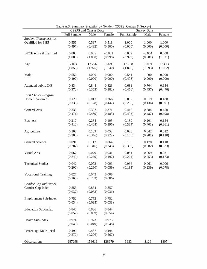
technical or vocational institute. (Appendix Table A.3 presents the full summary statistics.)

Figure 2 displays differences in male and female choices by performance on the Basic Education

Certification Exam. Each subfigure indicates the share of male and female students in each

BECE score decile who selected a given programme as their first choice (we include students

who fail to qualify for secondary school at 0). There is a strong exam score gradient in choices,

with 36 per cent of female students who did not qualify for secondary school admission choosing

home economics compared to only 2.2 per cent of female students in the top BECE decile.

Similarly, higher performing students are less likely to select technical or vocational studies and

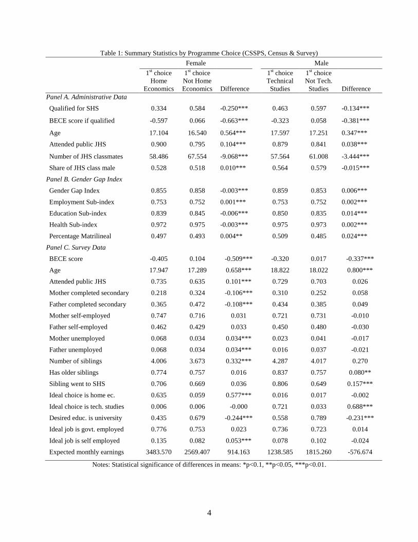
agriculture but are more likely to select general sciences. Table 1 provides an additional set of

summary statistics, which highlights differences in characteristics of students who pick home

economics and technical or vocational studies as their first choice programmes. It is also clear

here that there is negative selection into home economics by academic performance. Students

who choose home economics are less likely to have qualified for secondary school and have

lower exam scores when they do qualify. They are also older than other students and more likely

to have attended a public school.

Figure 3 reveals substantial geographic differences in programme choices. We plot the share of

male and female students selecting a programme by district. The share of all female students

picking home economics ranges from 2 per cent of students in East Gonja district in the Northern

Region to 52 per cent of students in Abura/Asebu/Kwamankese district in the Central Region.

These differences in choices persist even after controlling for academic performance. For

example, Appendix Figure A.1 demonstrates the variation in choices among the set of students

who did not qualify for admission to secondary school. The share of students selecting home

economics among this group still ranges from 2 to 57 per cent of female students in a district. In

Panel B of Table 1, we report the average levels of gender parity as measured by our gender gap

index. The differences among female students indicate that students who choose home

economics tend to come from areas with lower levels of gender parity. Conversely, male students

who pick technical studies tend to come from areas with higher levels of gender parity.

This preliminary examination of gender choices establishes a clear difference in the choices of

male and female students, but also highlights systematic variation in programme choices within

the two genders. The fact that low-performing female students and students from areas with

lower levels of gender parity are more likely to choose home economics could reflect a causal

relationship between academic potential and programme choices, but could alternatively reflect

the prevalence of social norms that place a low value on female student achievement and

encourage girls to pursue gender stereotypic courses. We now proceed to examine alternative

explanations for the observed patterns of gender differences in programme choices using a series

of linear regressions.

5 Explaining Gender Differences in Programme Choices

We begin our regression analysis by focusing on individual-level factors, primarily academic

performance. We then look at school environments, family backgrounds, and finally at

community-level characteristics. Our basic regression specification takes the form:

Yi = α0 + α1Femalei + Xi α2 + εi

where programme choice Yi for student i is estimated to be a function of a Femalei indicator

variable for student sex and a vector of covariates, Xi. We focus on home economics and

technical studies as our main programme choices of interest because these are the two most

gender segregated fields of study. We include region fixed effects in all of our regressions to

account for aggregate differences across the ten administrative regions in Ghana and cluster our

standard errors at the district level to allow for correlations in unobserved factors within districts.

Table 2 presents results from our baseline ordinary least squares regression. Panel A reports

results estimating the probability of choosing home economics. Panel B reports results

estimating the probability of choosing technical studies. Column 1 presents the correlation

between gender and choices for the full sample and column 2 repeats the regression for students

who do not qualify for secondary school admission. The coefficient on the female indicator

variable increases from 0.250 to 0.339 for home economics going from column 1 to column 2,

and decreases from -0.072 to -0.092 for technical studies, indicating that gender differences in

choices are larger among low performing students. Columns 3 and 4 focus on students who

qualify for secondary school and show that there is a significant decrease in the likelihood of

picking home economics or technical studies for higher performing students. Finally, column 5

restricts the sample to females in Panel A and males in Panel B, to estimate the BECE gradient in

choices within genders. Variation in BECE scores is a bigger determinant of variation in female

choices than male choices, and accounts for over three times as much variation for females. The

R2 is rather low in both cases, 0.071 for females and 0.023 for males, indicating that exam scores

alone explain relatively little of the overall variation in the likelihood of choosing a gender-

specific programme for students of a given gender.

5.1 Individual Academic Performance

Although statistically significant, the negative correlation between BECE performance and the

probability of choosing a gender-specific programme does not necessarily indicate that low

academic performance causes students to choose home economics or technical studies. To isolate

the effect of academic potential on student choices, we construct a proxy sample of siblings

(twins and triplets) and estimate a set of within-family regressions:

Yif = β0 + β1Femaleif + β2BECEif + ηf + εif

Here, we estimate programme choice for student i in family f to be a function of students’ sex

and BECE scores. We also include a family fixed effect, ηf. The motivation behind this analysis

is that it provides an opportunity to examine the choices of students who share the same family

environment and presumably would have been exposed to the same social norms and parental

preferences. Our assumption is that differences in the BECE performance of siblings are more

likely to reflect differences in intrinsic academic ability. We therefore interpret subsequent

differences in programme choices as reflecting the relationship between perceived academic

potential and desired programme choice. Since we do not explicitly observe family members, we

create a proxy measure by identifying students who share the same last name and date of birth

and who attended the same junior high school. These selection criteria result in a sample of 3,205

twins or triplets. Table A.4 reports basic summary statistics for students in this sample.

We find that gender differences hold within families and that lower-performing siblings are

significantly more likely to choose home economics (Table 3). This provides additional support

for the theory that lower-performing female students choose to pursue home economics because

it has relatively easier course requirements and is perceived to be less academically challenging

than other programmes. The same pattern holds for male students and the choice of technical

studies, although the coefficient on BECE scores is no longer significant once we include family

fixed effects. Strikingly, including family fixed effects in our regressions increases the R2 from

0.1 or less in most specifications to over 0.7. This indicates that unobserved factors that vary at

the family-level are a strong predictor of schooling choices. Overall, variation in exam

performance explains a higher percentage of variation in programme choices for female students

than for males once again.

5.2 School Environment

We move on to explore the relationship between school environments and student choices, and

estimate a separate set of regressions for male and female students. In doing so, we analyse the

correlation between individual-level programme choice and observable student and school

characteristics. Our linear regressions take the following form:

Yigs = γ0 + γ1BECEigs + Xigsγ2 + Zsγ3 + εigs

where Yigs is an indicator for student i of gender g in school s selecting a gender-specific

programme, BECEigs is the student’s score on the BECE exam, Xigs is a set of student

characteristics and Zs a set of junior high school characteristics.

Table 4 presents the results of this analysis. The first two columns include the full sample of

students and estimate the relationship between qualifying for secondary school admission and

programme choices. Qualifying for secondary school admission has a significant negative

correlation with choosing home economics and technical studies. Controlling for school

characteristics in column 2 reduces the size of the coefficient on qualifying for admission from -

0.167 to -0.132 for home economics and from -0.034 to -0.028 for technical studies, but the

coefficients remain statistically significant at the 1 per cent level in all cases. We focus on

students who did not qualify for secondary school in column 3 and school characteristics explain

2.4 to 3.3 per cent of the variation in programme choices. We restrict the sample to students who

qualified for secondary school in columns 4 and 5, and can now include BECE exam scores. The

coefficient on exam scores remains negative and significant once we add controls for JHS

characteristics. Under all specifications, students who attend public JHSs are significantly more

likely to choose home economics. Additionally, there is a positive correlation between the share

of JHS classmates who are male and whether a female chooses home economics. This is

consistent with existing literature that demonstrates that gender stereotypes become more

pronounced for females in coeducational environments (for example, Favara, 2012; Schneeweis

and Zweimüller, 2012; and Anelli and Peri, 2013), but we take this as only a suggestive

indication of the importance of social norms because differences in the gender compositions of

schools may reflect other underlying factors. Conversely, male students are less likely to choose

technical studies as the share of their male classmates increases, suggesting that gender

stereotypes weaken for males in a more single-sex environment.

One additional potential role of schooling environments is that school-based networks could

serve as important sources of information. We intend to explore this possibility in future work by

using school fixed effects to characterise the types of information that students were likely to

have received, given the historical programme choices and post-secondary outcomes of students

who had previously attended their schools.

5.3 Family Background

Having examined the role of school-level factors, our next objective is to analyse the extent to

which family characteristics are correlated with the programme choice decision. We turn now to

using the survey data. Our main specification is:

Yi = δ0 + δ1Femalei + δ2BECEi + Xiδ3 + εi

where Xi is a set of family background characteristics. Table 5 presents the results. Columns 1 to

3 focus on the choice of home economics. The coefficient on the gender indicator variable

remains significant and positive and the magnitude is quite similar to that estimated using the

2005 CSSPS data in Table 2 even though the two samples are separated by a period of 7 years

(female students in the survey sample are 17.5 percentage points more likely to pick home

economics than males and the corresponding gender difference was 16.3 percentage points in the

sample of students who qualified for admission to secondary school in 2005). Family-level

factors such as parents’ education and number of siblings do not appear to significantly predict

the choice of home economics, although the signs of the coefficients indicate that better educated

parents are less likely to have children who select home economics as their first choice

programme. We also look at parents’ employment and find that students with a mother who is

unemployed are more likely to select home economics. Moreover, students with mothers who

work for an international organization are significantly less likely to select home economics.

Both of these results are consistent with the general pattern that students who come from more

privileged backgrounds are less likely to select home economics.

The remaining columns of Table 5 report results for the choice of technical studies. Here, we

find that students with mothers who attended secondary school are more likely to choose

technical studies. Additionally, students with fathers who work for an international organization

are less likely to select technical studies. This accounts for a small share of the sample, however,

as less than 2 per cent of students have a parent who works for an international organization. The

one consistently significant relationship we find across the two programme choices is that having

an older sibling who attended secondary school is associated with having a higher probability of

selecting a gender-specific field of study. We do not have a clear explanation for this finding but

one possibility is that students experience less pressure to pursue an academically challenging

field of study if they have an older sibling who has already attended secondary school.

Altogether, family background characteristics only marginally increase our ability to explain

variation in programme choices. Including the full set of family characteristics increases the R2

on the home economics regression from 0.100 (with a female indicator and region fixed effects

only) to 0.120 and increases the R2 on the technical studies regression from 0.041 to 0.057.

5.4 District Characteristics

Our final empirical exercise examines district-level sources of heterogeneity in choices.

Appendix Figure A.2 illustrates the geographical variation in our measures of gender parity.

Figure A.3 plots the correlation between the district-level gender gap index (GGI) and: i) the

share of female students choosing home economics as a first choice programme, ii) the share of

male students choosing technical studies as a first choice programme, and iii) the female-male

ratio of BECE performance. In order to examine these correlations more systematically, we

estimate an additional set of regressions that capture the relationship between district-level

programme choices and district-level measures of gender parity:

Ydr = θ0 + θ1GenderGapIndexd + ρr + εdr

where Ydr is the share of students in district d and region r who chose a gender-specific

programme or the female-male BECE score ratio. GenderGapIndexd is our district-level measure

of gender parity, which gets closer to one as gender parity increases. Finally, ρr is a region fixed

effect.

Table 6 presents the results of this analysis. Column 1 of Panel A reports the raw correlation

between the district-level GGI and percentage of females choosing home economics. There is no

significant relationship between the two. We add region fixed effects to our specification in

column 2 and the R2 on this regression increases to 0.372 from 0.035 in the previous regression,

indicating that region-specific factors account for a third of the cross-district variation in

programme choices. Nonetheless, within-region differences in levels of gender parity now

significantly explain part of the variation in programme choices. The coefficient on the gender

gap index becomes negative, with a magnitude of -0.598, significant at the 1 per cent level. To

put the magnitude of this coefficient into perspective, moving from the least gender equal to the

most gender equal district in the country (a 0.234 point change in the GGI) would be associated

with a 14 percentage point decrease in the share of female students choosing home economics.

Thus, the percentage of females choosing home economics dramatically decreases in districts

with greater gender parity when we hold region-level factors constant and look at variation in

gender parity within regions.

In columns 3 to 5, we split the index into its three components and find that the level of parity in

educational attainment for men and women in a district largely drives the negative GGI

correlation. This result is robust to adding a control for the mean female BECE score in each

district (column 6), and becomes stronger when we estimate a population-weighted regression to

account for the fact that certain districts represent a larger number of students than others

(column 7). A population-weighted estimate of the regression in column 1 also yields a

significant negative coefficient on the gender gap index, with a magnitude of -0.461, significant

at the 10 per cent level.

We look at male choices in Panel B. The raw correlation between the GGI and probability of

males choosing technical studies is positive and significant (column 1), but shrinks close to 0 and

becomes insignificant once we include region fixed effects (column 2). When we examine the

coefficients on the individual components of the gender gap index (columns 3 to 7), we find a

positive and significant coefficient on the education sub-index. Male students in places with

more gender equality in educational attainment are more likely to choose technical studies.

In Panel C, we take the relative BECE scores of females and males in a district as our outcome

variable. The higher the GGI, the higher female exam scores are relative to males. Once again,

we find the strongest correlation between the education sub-index and gender parity in BECE

scores. Although the direction of causality cannot be determined, these results demonstrate that

areas with higher levels of gender equality in educational attainment also have higher performing

females who are less likely to choose home economics. Additionally, places with a higher

proportion of the population from the only matrilineal ethnic group in Ghana (Akans) also have

higher levels of gender parity in BECE performance.

To account for cross-district differences in academic performance, we include controls for the

mean BECE scores of students in the final columns of Panel A and B, and the results are

unchanged. We also estimate the same set of regressions but with the share of non-qualifying

students who pick home economics and technical studies as our dependent variables (Appendix

Table A.5). The results still indicate a significant negative correlation between the GGI and share

of female students choosing home economics, but no significant correlation for male students.

5.5 Robustness Checks

So far, our empirical analysis has documented that individual academic performance strongly

predicts programme choice, even after controlling for a host of other factors. We conduct a series

of exercises in the remainder of this section to check the robustness of our main results.

Table A.6 looks at strategic behaviour. Examining a student’s first choice might not capture

actual preferences because students may be strategic about what programme they list in order to

increase their admission chances. To address this concern, we estimate an additional set of

regressions with three alternative outcomes: i) an indicator for selecting home economics or

technical studies for any of the listed choices; ii) an indicator for selecting the programme for all

of the listed choices; and iii) an indicator for selecting the programme as an ideal first choice

(from survey responses to the following question: “Now, imagine that you can select any three

choices based on how much you liked them and without thinking about the school categories or

your chances of getting admitted to the course or anything else. What schools and courses would

you pick?”) Our results are robust to these alternative indicators of student choices, with the one

exception that BECE scores are not a significant predictor of listing technical studies for all

choices for students in the survey sample (column 6 of Panel B).

Table A.7 looks at changes in choices over time using the first five years of administrative data

(from 2005 to 2009). There has been a steady increase in the proportion of female students

selecting home economics and a decline in the proportion of students selecting technical studies.

Moreover, Figures A.4 and A.5 in the appendix indicate that the BECE score gradient has been

flattening over time, with an increasing share of high-performing female students selecting home

economics instead of general science. These changing patterns may in part reflect students’

strategic responses to the merit-based admission system that generates a separate BECE score

cut-off for each programme in a given school. Thus, a high achieving student who lists home

economics as her first choice stands a better chance of admission to a selective school than if she

applied for general science at that same school, for example. Despite the potential for strategic

behaviour, we still find that higher performing students are less likely to select gender-specific

fields of study as their first choice programme in all years for which we have data.

Table A.8 reports students’ favourite subjects in junior high school using responses from the

student survey. Students who choose home economics are less likely to report Mathematics and

Science as their best subjects but more likely to list Social Studies (Table A.11). This is

consistent with our interpretation that students are likely to be choosing secondary school

programmes based on their academic potential and their likelihood of succeeding in or enjoying

a given field of study.

6 Implications

We return here to the question of why gender differences in programme choices matter. To our

knowledge there are no longitudinal studies on the relationship between field of study and post-

schooling outcomes of individuals in Ghana. Nonetheless, cross-country studies show that

women in developing countries are more likely to work as unpaid labourers and in informal

sector jobs where they earn lower wages (World Bank, 2012). To draw some inferences about

potential links between programme choice and future employment, we turn again to our survey

data.

The survey captures desired educational attainment and future careers for all respondents. Tables

A.9 and A.10 display the link between these desires and current programme choice. Females

choosing home economics are less likely than students choosing other programmes of study to

plan on attending university. The same pattern is evident for males who choose technical studies.

Most of the females choosing home economics intend to pursue careers in nursing or in the

hospitality industry (hotel or restaurant work), neither of which requires a university degree.

Tables A.11 and A.12 present these differences in a set of regressions that control for student

BECE scores, age, and attending a public JHS.

There are several alternative explanations for our main results about gender differences in

programme choices. One possibility is that students differ in their knowledge about the existence

of and returns to different fields, or may lack exposure to people who have studied them. To

explore this possibility, we use the fact that our survey respondents were asked to indicate their

expected monthly earnings following secondary school. On average, students expect to earn over

twice the minimum wage (Figure A.6). Nonetheless, the median expected wage for females was

the same across all programme choices except for students choosing technical studies and

agriculture, who expected to earn higher wages. Male students pursuing technical studies,

agriculture, and business expected to earn substantially more than students who chose any of the

other programmes. The fact that female students pursuing home economics do not expect to earn

lower wages than students pursuing other fields suggests that these students do not anticipate any

negative wage implications as a result of pursuing a traditionally female-dominated field.

7 Conclusions

This paper provides new insights into the patterns and sources of gender differences in schooling

choices. We analyse the programme choices of secondary school applicants in Ghana and

document that female students segregate into studying home economics while male students

segregate into technical studies. However, these aggregate gender differences in programme

choices mask substantial underlying variation based on students’ academic performance and

prevailing educational norms. Higher performing female students and those from districts with a

history of gender parity in educational attainment are significantly less likely to choose home

economics.

Despite the robustness of our main findings, we cannot fully explain why male and female

students have such different preferences for fields of study. The low R2 on our linear regressions

indicates that the detailed set of variables we include in our analysis does not identify the

fundamental determinants of students’ schooling choices. In particular, unobserved aggregate

level factors (captured by region fixed effects) and unobservable variation across families

(captured by family fixed effects) explain more of the differences in programme choice than we

can explain using specific individual, school, or family level characteristics. Additionally, our

econometric models generally do a better job of explaining variation in the choices of female

students than those of males.

There are several alternative explanations that are consistent with our results and could account

for the gender differences in programme choices that we describe. These alternative pathways

suggest three additional areas for future research. First, we do not measure social norms directly

but instead proxy for these by looking at differences in application behaviour across families and

across geographic areas with different prevailing levels of gender parity. Future studies could

explicitly assess the role of social norms by measuring them directly; for example, by using

survey questions to assess respondents’ agreement with various statements about gender

stereotypes. Second, future work could explore the extent to which income levels in a family or

geographic location affect schooling choices. Indeed, some of the observable characteristics we

analyse suggest that income constraints might impact programme choices because mothers’

employment reduces the likelihood of choosing home economics, but we are unable to test this

hypothesis because we do not have direct measures of family income. Third, concerns about

childbearing and family responsibilities could influence programme choices. Women bear the

brunt of childrearing and home production in most parts of the world. Future work could assess

whether access to contraceptives and family friendly arrangements in the labour market

encourage women to pursue non-traditional fields of study.

Finally, this study exposes the need for further research to directly establish the link between

fields of study and the post-schooling outcomes of youth in developing countries. We show that

students’ programme choices significantly predict their educational and career aspirations but we

cannot definitively determine how pursuing a gender stereotypical programme ultimately affects

the livelihoods of men and women in Ghana. Future work to establish this relationship would

provide a platform for ensuring that the recent gains in female educational attainment worldwide

translate into improvements in women’s social and economic wellbeing.

1 This excludes only the small number of private international schools that do not follow the

SSCE curriculum and have their own application and admission procedures. 2 The World Economic Forum reported a GGI score of 0.665 for Ghana when it was first

included in the Global Gender Gap Report in 2006 (Hausmann, Tyson, and Zahidi, 2006). Our

index differs primarily because we exclude the political empowerment component. The WEF

(our) values for the remaining sub-indices are 0.753 (0.748) for economic participation and

opportunity; 0.868 (0.813) for educational attainment; and 0.973 (0.963) for health and survival.

The WEF primarily used the UN Human Development Report, WHO World Health Statistics,

and ILO LABORSTA database to construct their indices, whereas we use the 2000 census and

2005 Ghana Living Standards Survey (for information on employment income) in order to

capture district-level variation.

1

Figure 1: Gender Differences in Programme Choices (CSSPS)

Notes: Figure illustrates proportion of secondary school applicants who selected each programme as their first

choice in 2005.

2

Figure 2: Academic Performance and Programme Choices (CSSPS)

Notes: Figures illustrate proportion of secondary school applicants who selected each programme as their first

choice, by their decile of performance on the Basic Education Certification Exam. Students who fail to qualify for

admission to secondary school are included at 0. Female students comprise 48.3 per cent of students who do not

qualify for secondary school and 38.3 per cent of students in the top BECE decile.

3

Figure 3: Geographic Differences in Programme Choices (CSSPS)

Notes: Figures illustrate district-level variation in the proportion of secondary school applicants who selected each

programme as their first choice.

4

Table 1: Summary Statistics by Programme Choice (CSSPS, Census & Survey)

Female Male

1st choice 1

st choice 1

st choice 1

st choice

Home

Economics

Not Home

Economics

Difference

Technical

Studies

Not Tech.

Studies

Difference

Panel A. Administrative Data

Qualified for SHS 0.334 0.584 -0.250*** 0.463 0.597 -0.134***

BECE score if qualified -0.597 0.066 -0.663*** -0.323 0.058 -0.381***

Age 17.104 16.540 0.564*** 17.597 17.251 0.347***

Attended public JHS 0.900 0.795 0.104*** 0.879 0.841 0.038***

Number of JHS classmates 58.486 67.554 -9.068*** 57.564 61.008 -3.444***

Share of JHS class male 0.528 0.518 0.010*** 0.564 0.579 -0.015***

Panel B. Gender Gap Index

Gender Gap Index 0.855 0.858 -0.003*** 0.859 0.853 0.006***

Employment Sub-index 0.753 0.752 0.001*** 0.753 0.752 0.002***

Education Sub-index 0.839 0.845 -0.006*** 0.850 0.835 0.014***

Health Sub-index 0.972 0.975 -0.003*** 0.975 0.973 0.002***

Percentage Matrilineal 0.497 0.493 0.004** 0.509 0.485 0.024***

Panel C. Survey Data

BECE score -0.405 0.104 -0.509*** -0.320 0.017 -0.337***

Age 17.947 17.289 0.658*** 18.822 18.022 0.800***

Attended public JHS 0.735 0.635 0.101*** 0.729 0.703 0.026

Mother completed secondary 0.218 0.324 -0.106*** 0.310 0.252 0.058

Father completed secondary 0.365 0.472 -0.108*** 0.434 0.385 0.049

Mother self-employed 0.747 0.716 0.031 0.721 0.731 -0.010

Father self-employed 0.462 0.429 0.033 0.450 0.480 -0.030

Mother unemployed 0.068 0.034 0.034*** 0.023 0.041 -0.017

Father unemployed 0.068 0.034 0.034*** 0.016 0.037 -0.021

Number of siblings 4.006 3.673 0.332*** 4.287 4.017 0.270

Has older siblings 0.774 0.757 0.016 0.837 0.757 0.080**

Sibling went to SHS 0.706 0.669 0.036 0.806 0.649 0.157***

Ideal choice is home ec. 0.635 0.059 0.577*** 0.016 0.017 -0.002

Ideal choice is tech. studies 0.006 0.006 -0.000 0.721 0.033 0.688***

Desired educ. is university 0.435 0.679 -0.244*** 0.558 0.789 -0.231***

Ideal job is govt. employed 0.776 0.753 0.023 0.736 0.723 0.014

Ideal job is self employed 0.135 0.082 0.053*** 0.078 0.102 -0.024

Expected monthly earnings 3483.570 2569.407 914.163 1238.585 1815.260 -576.674

Notes: Statistical significance of differences in means: *p<0.1, **p<0.05, ***p<0.01.

5

Table 2: Individual-Level Analysis of Gender Differences in Programme Choices (CSSPS)

Sample: All Not All All Qualified

Students Qualified Qualified Qualified A: Females

B: Males

(1) (2) (3) (4) (5)

Panel A. Home Economics

Female 0.250 0.339 0.164 0.163

(0.010)*** (0.010)*** (0.009)*** (0.008)***

BECE score -0.046 -0.105

(0.002)*** (0.005)***

R-squared 0.142 0.190 0.093 0.124 0.071

Observations 287298 127603 159695 142485 58086

Panel B. Technical Studies

Female -0.072 -0.092 -0.058 -0.061

(0.007)*** (0.012)*** (0.006)*** (0.006)***

BECE score -0.017 -0.027

(0.001)*** (0.003)***

R-squared 0.038 0.055 0.029 0.037 0.023

Observations 287298 127603 159695 142485 84399

Notes: All regressions include region fixed effects. Robust standard errors clustered at the JHS district level are

reported in parentheses. Coefficient statistical significance: *p<0.1, **p<0.05, ***p<0.01.

6

Table 3: Sibling Analysis of Gender Differences in Programme Choices (CSSPS)

Sample: All All Not Not All All Qualified Qualified

Siblings Siblings Qualified Qualified Qualified Qualified A: Sisters A: Sisters

B: Brothers B: Brothers

(1) (2) (3) (4) (5) (6) (7) (8)

Panel A. Home Economics

Female 0.225 0.261 0.328 0.307 0.151 0.162

(0.013)*** (0.033)*** (0.023)*** (0.080)*** (0.015)*** (0.045)***

BECE score -0.045 -0.104 -0.069 -0.218

(0.006)*** (0.034)*** (0.014)*** (0.113)*

Family Fixed Effects No Yes No Yes No Yes No Yes

R-squared 0.111 0.694 0.162 0.798 0.105 0.719 0.039 0.718

Observations 3205 3205 1252 1252 1651 1651 520 520

Panel B. Technical Studies

Female -0.073 -0.095 -0.095 -0.145 -0.065 -0.065

(0.007)*** (0.020)*** (0.014)*** (0.053)*** (0.009)*** (0.029)**

BECE score -0.009 -0.010 -0.016 -0.033

(0.004)** (0.020) (0.010) (0.040)

Family Fixed Effects No Yes No Yes No Yes No Yes

R-squared 0.035 0.653 0.048 0.729 0.031 0.768 0.004 0.795

Observations 3205 3205 1252 1252 1651 1651 669 669

Notes: All regressions are run with robust standard errors, clustered at the family level. Coefficient statistical significance: *p<0.1, **p<0.05, ***p<0.01. Odd

columns replicate baseline analysis from Table 2 and even columns include family fixed effects to account for unobserved family-specific factors that influence

schooling choices.

7

Table 4: School Environment (CSSPS)

Sample: All All Not All All

Students Students Qualified Qualified Qualified

(1) (2) (3) (4) (5)

Panel A. Home Economics (Females only)

Qualified for SHS -0.167 -0.132

(0.009)*** (0.009)***

BECE score -0.098 -0.146

(0.005)*** (0.008)***

JHS Public 0.037 0.063 0.027

(0.007)*** (0.013)*** (0.006)***

Number of JHS classmates -0.000 -0.000 -0.000

(0.000) (0.000) (0.000)***

Median score in JHS -0.046 -0.041 0.086

(0.006)*** (0.014)*** (0.007)***

Share of JHS classmates male 0.066 0.049 0.055

(0.022)*** (0.031) (0.022)**

Region Fixed Effects Yes Yes Yes Yes Yes

R-squared 0.067 0.074 0.024 0.075 0.086

Observations 125795 125795 59221 58063 58063

Mean Outcome 0.264 0.264 0.368 0.177 0.177

Panel B. Technical Studies (Males only)

Qualified for SHS -0.034 -0.028

(0.009)*** (0.008)***

BECE score -0.024 -0.039

(0.002)*** (0.003)***

JHS Public 0.020 0.031 0.011

(0.004)*** (0.010)*** (0.003)***

Number of JHS Classmates -0.000 -0.000 -0.000

(0.000) (0.000)* (0.000)

Median score in JHS -0.007 -0.006 0.030

(0.003)** (0.006) (0.004)***

Share of JHS Classmates male -0.045 -0.065 -0.039

(0.014)*** (0.020)*** (0.015)***

Region Fixed Effects Yes Yes Yes Yes Yes

R-squared 0.024 0.026 0.033 0.025 0.028

Observations 154520 154520 61530 84372 84372

Mean Outcome 0.073 0.073 0.096 0.059 0.059

Notes: All regressions are run with robust standard errors, clustered at the district level. Regressions also include

region fixed effects and controls for student age. Coefficient statistical significance: *p<0.1, **p<0.05, ***p<0.01.

8

Table 5: Family Background (Survey)

Programme Choice Home Economics Technical Studies (1) (2) (3) (4) (5) (6)

Female 0.171 0.175 0.175 -0.054 -0.049 -0.050 (0.017)*** (0.017)*** (0.017)*** (0.014)*** (0.013)*** (0.013)*** BECE score -0.033 -0.032 -0.009 -0.012 (0.007)*** (0.007)*** (0.004)* (0.004)** Age

0.007 0.007 0.008 0.009 (0.003)** (0.003)** (0.003)** (0.003)**

Attended public JHS

-0.003 -0.003 -0.005 -0.004 (0.006) (0.007) (0.004) (0.003)

Mother completed secondary

-0.002 0.016 (0.018) (0.006)**

Father completed secondary

-0.004 0.003 (0.011) (0.007)

Mother unemployed

0.060 -0.017 (0.028)* (0.013)

Mother self-employed

0.009 -0.008 (0.023) (0.020)

Mother govt. employed

-0.015 -0.007 (0.022) (0.018)

Mother privately employed

-0.015 -0.016 (0.021) (0.022)

Mother works for int'l org

-0.127 0.052 (0.037)*** (0.074)

Father govt. employed

0.006 0.012 (0.022) (0.009)

Father privately employed

0.016 0.010 (0.020) (0.012)

Father works for int'l org

0.022 -0.038 (0.044) (0.021)*

Number of siblings

0.001 0.001 (0.002) (0.001)

Has older siblings

-0.021 -0.004 (0.019) (0.010)

Sibling went to SHS

0.029 0.027 (0.013)** (0.009)**

Father self-employed

-0.005 0.002 (0.021) (0.013)

Father unemployed

0.045 -0.002 (0.042) (0.018)

R-squared 0.100 0.114 0.120 0.041 0.049 0.057 Observations 3933 3933 3933 3933 3933 3933 Notes: All regressions include region fixed effects. Robust standard errors clustered at the JHS region level are

reported in parentheses. Coefficient statistical significance: *p<0.1, **p<0.05, ***p<0.01.

9

Table 6: District-Level Analysis of Gender Differences in Programme Choices (CSSPS & Survey)

(1) (2) (3) (4) (5) (6) (7) Panel A. Percentage of Females Choosing Home Economics

Gender Gap Index -0.007 -0.598 (0.247) (0.215)*** Economic Sub-index -0.294 -0.190 0.048 (0.185) (0.177) (0.184) Education Sub-index -0.361 -0.253 -0.363 (0.141)** (0.138)* (0.129)*** Health Sub-index -0.204 -0.097 -0.147 (0.140) (0.119) (0.121) Mean Female BECE Score -0.001 -0.001 (0.000)*** (0.000)*** Region Fixed Effects No Yes Yes Yes Yes Yes Yes Population Weighted No No No No No No Yes Observations 109 109 109 109 109 109 109 R-squared 0.000 0.384 0.349 0.381 0.351 0.435 0.466 Panel B. Percentage of Males Choosing Technical Studies

Gender Gap Index 0.191 0.033 (0.087)** (0.099) Economic Sub-index -0.109 -0.150 -0.016 (0.076) (0.078)* (0.108) Education Sub-index 0.101 0.128 0.128 (0.057)* (0.052)** (0.060)** Health Sub-index -0.013 -0.013 -0.028 (0.061) (0.059) (0.058) Mean Male BECE Score 0.000 0.000 (0.000) (0.000) R-squared 0.034 0.454 0.462 0.471 0.453 0.489 0.583 Panel C. BECE Score Ratio Gender Gap Index 0.564 0.374 (0.210)*** (0.219)* Economic Sub-index -0.077 -0.278 -0.083 (0.181) (0.188) (0.188) Education Sub-index 0.312 0.274 0.128 (0.123)** (0.129)** (0.118) Health Sub-index 0.158 0.126 0.006 (0.135) (0.125) (0.110) Per cent Matrilineal 0.097 0.079 (0.041)** (0.040)* R-squared 0.073 0.380 0.357 0.398 0.367 0.439 0.395 Notes: All regressions are run with robust standard errors, reported in parentheses. See Appendix Table A.2 for

details on Gender Gap Index subindices and weighting. All ratios consist of female measures in the numerator and

male measures in the denominator. Coefficient statistical significance: *p<0.1, **p<0.05, ***p<0.01.

10

References

Ajayi, K. F., & Telli, H. (2013). Imperfect Information and School Choice in Ghana, Working

paper.

Akerlof, G. A., & Kranton, R. (2002). Identity and Schooling: Some Lessons for the Economics

of Education, Journal of Economic Literature, 40(4), 1167–1201.

Akerlof, G. A., & Kranton, R. (2000). Economics and Identity, The Quarterly Journal of

Economics, 115, 715–753.

Anelli, M., & Peri, G. (2013). The Long Run Effects of High-School Class Gender Composition,

Working Paper 18744, National Bureau of Economic Research.

Arcidiacono, P. (2004). Ability Sorting and the Returns to College Major, Journal of

Econometrics, 121, 343–375.

Beffy, M., Fougère, D., & Maurel, A. (2012). Choosing the Field of Study in Postsecondary

Education: Do Expected Earnings Matter?, The Review of Economics and Statistics, 94(1),

334–347.

Bharadwaj, P., De Giorgi, G., Hansen, D. & Neilson, C. (2012). The Gender Gap in

Mathematics: Evidence from Low- and Middle-Income Countries, Working Paper 18464,

National Bureau of Economic Research.

Buser, T., Niederle, M., & Oosterbeek, H. (2012). Gender, Competitiveness and Career Choices,

Working Paper 18576, National Bureau of Economic Research.

Favara, M. (2012). The Cost of Acting “Girly”: Gender Stereotypes and Educational Choices,

11

IZA Discussion Papers 7037, Institute for the Study of Labor (IZA).

Fryer, R. G., & Levitt, S. D. (2010). An Empirical Analysis of the Gender Gap in Mathematics,

American Economic Journal: Applied Economics, 2(2), 210–240.

Ghana Statistical Service (2005). Ghana Living Standards Survey: Version 2.0 [Dataset]. Accra:

Ghana Statistical Service.

Goldin, C., Katz, L. F., & Kuziemko, I. (2006). The Homecoming of American College Women:

The Reversal of the College Gender Gap, Journal of Economic Perspectives, 20(4), 133–56.

Guiso, L., Monte, F., Sapienza, P., & Zingales, L. (2008). Culture, Gender, and Math, Science,

320, 1164–1165.

Hausmann, R., Tyson, L. D., & Zahidi, S. (2006). The Global Gender Gap Report 2006. Geneva:

World Economic Forum.

Hausmann, R., Tyson, L. D., & Zahidi, S. (2009). The Global Gender Gap Report 2009. Geneva:

World Economic Forum.

Jensen, R. (2012). Do Labor Market Opportunities Affect Young Women’s Work and Family

Decisions? Experimental Evidence from India, The Quarterly Journal of Economics, 27,

753-792.

Minnesota Population Center (2013). Integrated Public Use Microdata Series, International:

Version 6.2 [Machine readable database]. Minneapolis: University of Minnesota.

Munshi, K., & Rosenzweig, M. (2006). Traditional Institutions Meet the Modern World: Caste,

Gender, and Schooling Choice in a Globalizing Economy, American Economic Review, 96,

12

1225–1252.

Oster, E., & Millett, B. (2013). Do IT Service Centers Promote School Enrollment? Evidence

from India, Journal of Development Economics, 104, 123-135

Pope, D. G., & Sydnor, J. R. (2010). Geographic Variation in the Gender Differences in Test

Scores, Journal of Economic Perspectives, 24(2), 95–108.

Schneeweis, N., & Zweimüller, M. (2012). Girls, Girls, Girls: Gender Composition and Female

School Choice, Economics of Education Review, 31(4), 482–500.

Turner, S. E., & Bowen, W. G. (1999). Choice of Major: The Changing (Unchanging) Gender

Gap, Industrial and Labor Relations Review, 52, 289–313.

Wiswall, M., & Zafar, B. (2011). Determinants of College Major Choice: Identification Using an

Information Experiment, Staff Reports 500, Federal Reserve Bank of New York.

World Bank (2012). World Development Report 2012: Gender Equality and Development.

Washington, DC: The World Bank.

Zafar, B. (2013). College Major Choice and the Gender Gap, Journal of Human Resources, 48,

545–595.

1

Online Appendix

Figure A.1: Geographic Differences in Programme Choices (Unsuccessful Applicants, CSSPS)

Notes: Figures illustrate district-level variation in the percentage of unsuccessful secondary school applicants who

selected each programme as their first choice.

2

Figure A.2: Geographic Differences in Gender Parity (Census)

Notes: Figures illustrate district-level variation in gender parity indicators, constructed using data from

2000 census and 2005 Ghana Living Standards Survey.

3

Figure A.3: District-Level Correlations (CSSPS & Census)

Notes: Figures illustrate correlation between district-level measures of gender parity and a) female likelihood of

choosing Home Economics, b) male likelihood of choosing Technical Studies, and c) female-male ratio of BECE

performance.

4

Figure A.4: Academic Performance and Programme Choices by Year (Females, CSSPS)

Notes: Figures illustrate percentage of secondary school applicants who selected each programme as their first

choice, by their decile of performance on the Basic Education Certification Exam. Students who fail to qualify for

admission to secondary school are included at 0.

5

Figure A.5: Academic Performance and Programme Choices by Year (Males, CSSPS)

Notes: Figures illustrate percentage of secondary school applicants who selected each programme as their first

choice, by their decile of performance on the Basic Education Certification Exam. Students who fail to qualify for

admission to secondary school are included at 0.

6

Figure A.6: Median Expected monthly wage after completing secondary school (Survey)

Notes: Figure reports wage expectations in GHc. Minimum wage = GHc 90/month and GHc 2 ≈ $1 at the time of

the survey in 2012.

7

Table A.1: Course Requirements for Secondary School Programmes

Programme Required Courses Elective Courses

General Arts 1 of the following languages: 3 or 4 of the following:

French Christian Religious Studies Islamic Religious Studies

Dagaare, Dagbani, Geography Economics

Dangme, Ewe, Ga, Government Mathematics (Elective)

Gonja, Kasem, Nzema, History Music

Twi (Akuapem), Literature-in-English

Twi (Asante)

General Science Mathematics (Elective) 2 or 3 of the following:

Biology

Chemistry

Physics

French OR Music

Geography

Home Economics Management-In-Living 1 of the following: 1 of the following: 1 of the following:

Clothing and Textiles General Knowledge-In-Art Biology

Foods and Nutrition Textiles Chemistry

French Physics

Economics Mathematics (Elective)

Technical Studies Technical Drawing 2 or 3 of the following:

Applied Electricity Electronics Mathematics (Elective)

Auto Mechanics Metalwork Physics

Building Construction Woodwork French

Notes: Table lists secondary school courses associated with four of the available programme choices. The West African Examination Council guidelines on exam

requirements state that: “The Core Subjects for the Secondary School Certification Examination are: English Language, Integrated Science, Mathematics (Core),

Social Studies. In addition to the Core Subjects, each candidate must choose ONE of the Options under ONE of the Programmes and must enter and sit for

THREE or FOUR Elective Subjects from the Option of his/her choice.” (http://www.ghanawaec.org/EXAMS/WASSCE.aspx, last accessed on June 2, 2014.)

8

Table A.2: Gender Gap Index Component Summary Statistics (Census)

Mean SD SD per

1% change

Weight

Economic Opportunity

Ratio: Female to male employment rate 0.9583 0.0415 0.2412 0.5836

Ratio: Female to male prof. and tech. workers 0.5675 0.1230 0.0813 0.1967

Ratio: Female to male legislators and managers 0.7053 0.2201 0.0454 0.1100

Ratio: Female to male income from employment 0.7641 0.2205 0.0454 0.1098

Educational Attainment

Ratio: Female to male literacy rate 0.7021 0.1052 0.0950 0.2917

Ratio: Female to male net primary enrolment 0.9537 0.0623 0.1606 0.4931

Ratio: Female to male net secondary enrolment 0.7124 0.2556 0.0391 0.1201

Ratio: Female to male gross tertiary enrolment 0.5561 0.3228 0.0310 0.0951

Health and Survival

Ratio: Females to males under one year of age 0.9626 0.0587 0.1704 1.0000

9

Table A.3: Summary Statistics by Gender (CSSPS, Census & Survey)

CSSPS and Census Data Survey Data

Full Sample Male Female Full Sample Male Female

Student Characteristics

Qualified for SHS 0.556 0.587 0.518 1.000 1.000 1.000

(0.497) (0.492) (0.500) (0.000) (0.000) (0.000)

BECE score if qualified 0.000 0.035 -0.051 0.002 -0.004 0.008

(1.000) (1.000) (0.998) (0.999) (0.981) (1.021)

Age 17.014 17.276 16.690 17.768 18.071 17.413

(1.856) (1.975) (1.640) (1.820) (1.893) (1.662)

Male 0.552 1.000 0.000 0.541 1.000 0.000

(0.497) (0.000) (0.000) (0.498) (0.000) (0.000)

Attended public JHS 0.834 0.844 0.823 0.681 0.704 0.654

(0.372) (0.363) (0.382) (0.466) (0.457) (0.476)

First Choice Program

Home Economics 0.128 0.017 0.266 0.097 0.019 0.188

(0.335) (0.128) (0.442) (0.295) (0.136) (0.391)

General Arts 0.333 0.302 0.371 0.415 0.384 0.450

(0.471) (0.459) (0.483) (0.493) (0.487) (0.498)

Business 0.217 0.234 0.195 0.180 0.201 0.154

(0.412) (0.424) (0.396) (0.384) (0.401) (0.361)

Agriculture 0.100 0.139 0.052 0.028 0.042 0.012

(0.300) (0.346) (0.222) (0.166) (0.201) (0.110)

General Science 0.091 0.112 0.064 0.150 0.178 0.118

(0.287) (0.316) (0.245) (0.357) (0.382) (0.323)

Visual Arts 0.062 0.079 0.041 0.051 0.069 0.031

(0.240) (0.269) (0.197) (0.221) (0.253) (0.173)

Technical Studies 0.042 0.073 0.003 0.036 0.061 0.006

(0.200) (0.260) (0.059) (0.185) (0.239) (0.078)

Vocational Training 0.027 0.043 0.008

(0.163) (0.203) (0.086)

Gender Gap Indicators

Gender Gap Index 0.855 0.854 0.857

(0.032) (0.033) (0.031)

Employment Sub-index 0.752 0.752 0.752

(0.034) (0.035) (0.033)

Education Sub-index 0.840 0.836 0.844

(0.057) (0.059) (0.054)

Health Sub-index 0.974 0.973 0.975

(0.049) (0.049) (0.048)

Percentage Matrilineal 0.490 0.487 0.494

(0.272) (0.276) (0.267)

Observations 287298 158619 128679 3933 2126 1807

10

Table A.4: Sibling Summary Statistics (CSSPS)

Full Sibling Sisters Brothers

Sample Sample Only Only

(1) (2) (3) (4)

Student Characteristics Qualified for SHS

0.556 0.609 0.573 0.627 (0.497) (0.488) (0.495) (0.484)

BECE score if qualified

0.000 0.099 0.055 0.084 (1.000) (1.025) (1.028) (0.992)

Age 17.014 16.562 16.357 16.896 (1.856) (1.491) (1.339) (1.670) Male 0.552 0.513 0.000 1.000 (0.497) (0.500) (0.000) (0.000) Attended public JHS 0.834 0.837 0.834 0.860 (0.372) (0.369) (0.373) (0.347) Number of JHS classmates 62.720 69.121 70.285 64.873 (52.554) (56.439) (52.240) (54.729) Share of JHS class male 0.552 0.538 0.500 0.584 (0.119) (0.113) (0.102) (0.120) Gender Gap Indicators

Gender Gap Index 0.855 0.859 0.860 0.856 (0.032) (0.029) (0.027) (0.034) Percentage Matrilineal

0.490 0.474 0.483 0.464 (0.272) (0.266) (0.260) (0.277)

Sibling Characteristics

Sisters only

0.356 1.000 0.000 (0.479) (0.000) (0.000)

Brothers only

0.382 0.000 1.000 (0.486) (0.000) (0.000)

Mixed sex siblings

0.261 0.000 0.000 (0.440) (0.000) (0.000)

Both chose home ec 0.053 0.134 0.008 (0.225) (0.341) (0.090) None chose home ec 0.792 0.669 0.970 (0.406) (0.471) (0.171) Both chose tech 0.012 0.000 0.031 (0.111) (0.000) (0.173) None chose tech 0.933 0.995 0.895 (0.251) (0.072) (0.307) Observations 287298 3205 1142 1225

11

Table A.5: District-Level Analysis of Gender Differences in Programme Choices (Unsuccessful Applicants, CSSPS)

(1) (2) (3) (4) (5) (6) (7) Panel A. Percentage of Females Choosing Home Economics Gender Gap Index 0.182 -0.537

(0.293) (0.259)**

Economic Sub-index -0.354 -0.234 -0.101

(0.216) (0.223) (0.213)

Education Sub-index -0.267 -0.206 -0.294

(0.169) (0.178) (0.172)*

Health Sub-index -0.200 -0.122 -0.169

(0.155) (0.153) (0.161)

Region Fixed Effects No Yes Yes Yes Yes Yes Yes Population Weighted No No No No No No Yes Observations 109 109 109 109 109 109 109 R-squared 0.004 0.393 0.380 0.384 0.376 0.394 0.358 Panel B. Percentage of Males Choosing Technical Studies Gender Gap Index 0.230 0.036

(0.118)* (0.126)

Economic Sub-index -0.134 -0.183 -0.087

(0.099) (0.096)* (0.104)

Education Sub-index 0.155 0.196 0.234

(0.074)** (0.069)*** (0.073)***

Health Sub-index -0.052 -0.059 -0.062

(0.086) (0.082) (0.093)

R-squared 0.028 0.425 0.433 0.449 0.428 0.470 0.656 Notes: All regressions are run with robust standard errors, reported in parentheses. See Appendix Table A.2 for

details on Gender Gap Index subindices and weighting. All ratios consist of female measures in the numerator and

male measures in the denominator. Coefficient statistical significance: *p<0.1, **p<0.05, ***p<0.01.

12

Table A.6: Alternative Indicators of Programme Choices for Qualified Students (CSSPS &

Survey)

Administrative Data Survey Data

First Any All First Any All Ideal

Choice Choice Choices Choice Choice Choices Choice

(1) (2) (3) (4) (5) (6) (7)

Panel A. Home Economics

Female 0.163 0.414 0.043 0.175 0.311 0.153 0.153

(0.008)*** (0.011)*** (0.003)*** (0.017)*** (0.036)*** (0.017)*** (0.017)***

BECE score -0.046 -0.076 -0.010 -0.033 -0.052 -0.029 -0.029

(0.002)*** (0.002)*** (0.001)*** (0.007)*** (0.008)*** (0.005)*** (0.005)***

R-squared 0.124 0.283 0.032 0.116 0.230 0.106 0.106

Observations 142485 142485 142485 3933 3933 3933 3933

Mean Outcome 0.077 0.222 0.019 0.097 0.199 0.086 0.086

Panel B. Technical Studies

Female -0.061 -0.142 -0.012 -0.050 -0.153 -0.063 -0.063

(0.006)*** (0.009)*** (0.003)*** (0.013)*** (0.025)*** (0.017)*** (0.017)***

BECE score -0.017 -0.040 -0.003 -0.011 -0.027 -0.011 -0.011

(0.001)*** (0.002)*** (0.001)*** (0.004)** (0.007)*** (0.004)** (0.004)**

R-squared 0.037 0.078 0.010 0.056 0.132 0.068 0.068

Observations 142485 142485 142485 3933 3933 3933 3933

Mean Outcome 0.036 0.089 0.007 0.036 0.112 0.043 0.043

Notes: All regressions are run with region fixed effects and robust standard errors, clustered at the district level for

administrative data and at the regional level for the survey data. Survey data results include controls for parents'

education, the student's age and sibling characteristics. Coefficient statistical significance: *p<0.1, **p<0.05,

***p<0.01.

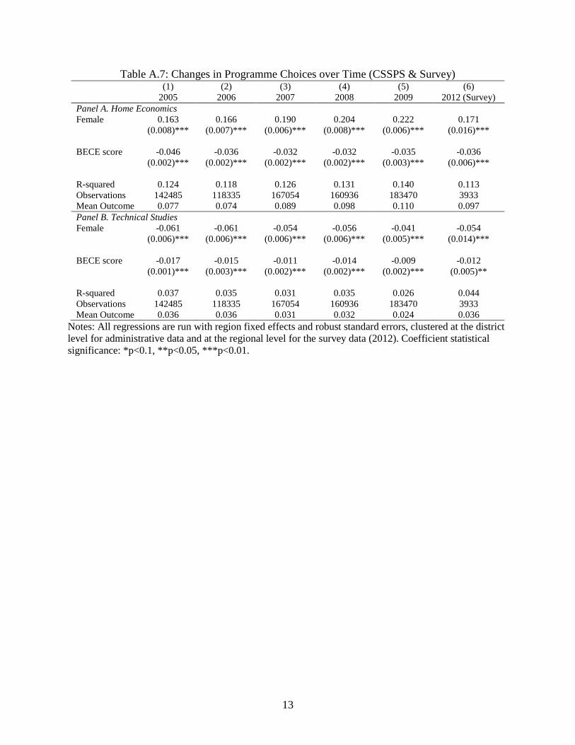
13

Table A.7: Changes in Programme Choices over Time (CSSPS & Survey) (1) (2) (3) (4) (5) (6)

2005 2006 2007 2008 2009 2012 (Survey)

Panel A. Home Economics

Female 0.163 0.166 0.190 0.204 0.222 0.171

(0.008)*** (0.007)*** (0.006)*** (0.008)*** (0.006)*** (0.016)***

BECE score -0.046 -0.036 -0.032 -0.032 -0.035 -0.036

(0.002)*** (0.002)*** (0.002)*** (0.002)*** (0.003)*** (0.006)***

R-squared 0.124 0.118 0.126 0.131 0.140 0.113

Observations 142485 118335 167054 160936 183470 3933

Mean Outcome 0.077 0.074 0.089 0.098 0.110 0.097

Panel B. Technical Studies

Female -0.061 -0.061 -0.054 -0.056 -0.041 -0.054

(0.006)*** (0.006)*** (0.006)*** (0.006)*** (0.005)*** (0.014)***

BECE score -0.017 -0.015 -0.011 -0.014 -0.009 -0.012

(0.001)*** (0.003)*** (0.002)*** (0.002)*** (0.002)*** (0.005)**

R-squared 0.037 0.035 0.031 0.035 0.026 0.044

Observations 142485 118335 167054 160936 183470 3933

Mean Outcome 0.036 0.036 0.031 0.032 0.024 0.036

Notes: All regressions are run with region fixed effects and robust standard errors, clustered at the district

level for administrative data and at the regional level for the survey data (2012). Coefficient statistical

significance: *p<0.1, **p<0.05, ***p<0.01.

14

Table A.8: Programme Choice and Favourite Subjects (Survey)

Panel A. Females Gen. Arts Gen. Sci Agric Business Tech. Home Ec. Vis. Arts Total

Mathematics 14.99 27.23 18.18 52.69 18.18 15.88 17.86 22.88

English 26.41 10.33 13.64 12.19 18.18 21.18 8.93 20.35

Integrated science 15.11 45.54 4.55 11.47 18.18 14.41 12.50 17.93

Social studies 22.73 7.04 36.36 9.32 18.18 22.35 26.79 18.85

Information and communication technology 1.72 2.82 4.55 1.79 0.00 2.94 1.79 2.13

French 1.72 1.88 4.55 2.51 9.09 0.88 1.79 1.79

Ghanaian language and culture 6.27 2.82 4.55 2.87 0.00 5.00 7.14 5.01

Religious and moral education 7.25 0.94 0.00 3.23 9.09 7.65 1.79 5.65

Basic design and technology 3.19 0.94 13.64 3.94 9.09 9.12 21.43 4.96

Missing 0.61 0.47 0.00 0.00 0.00 0.59 0.00 0.46

Total 814 213 22 279 11 340 56 1735

Panel B. Males Gen. Arts Gen. Sci Agric Business Tech. Home Ec. Vis. Arts Total

Mathematics 22.77 24.60 25.56 55.27 32.56 17.50 28.77 31.03

English 16.77 5.29 11.11 7.49 10.85 2.50 13.70 11.54

Integrated science 16.52 48.68 28.89 12.65 13.18 30.00 13.70 22.10

Social studies 27.29 10.32 15.56 12.65 17.05 25.00 17.81 19.14

Information and communication technology 2.94 3.97 2.22 3.28 3.10 2.50 5.48 3.35

French 2.08 1.06 1.11 0.47 1.55 0.00 2.05 1.43

Ghanaian language and culture 4.65 2.91 7.78 2.58 4.65 7.50 1.37 3.85

Religious and moral education 3.43 0.79 1.11 1.41 4.65 10.00 1.37 2.47

Basic design and technology 3.18 1.85 6.67 4.22 11.63 5.00 14.38 4.69

Missing 0.37 0.53 0.00 0.00 0.78 0.00 1.37 0.39

Total 817 378 90 427 129 40 146 2027

15

Table A.9: Programme Choice and Desired Educational Attainment (Survey)

Panel A. Females Gen. Arts Gen. Sci Agric Business Tech. Home Ec. Vis. Arts Total

Technical or vocational training 0.86 0.94 9.09 0.36 27.27 2.65 3.57 1.50

Senior high school 0.25 0.00 4.55 0.00 0.00 2.06 0.00 0.58

Nursing or teacher training 29.85 16.43 68.18 17.56 18.18 45.00 35.71 29.80

Polytechnic 3.19 0.94 0.00 4.30 27.27 5.29 1.79 3.57

University 65.60 80.75 18.18 77.06 27.27 43.53 57.14 63.86

Missing 0.25 0.94 0.00 0.72 0.00 1.47 1.79 0.69

Total 814 213 22 279 11 340 56 1735

Panel B. Males Gen. Arts Gen. Sci Agric Business Tech. Home Ec. Vis. Arts Total

Technical or vocational training 1.84 1.06 2.22 2.58 10.08 5.00 4.79 2.66

Senior high school 1.71 0.79 4.44 2.11 1.55 0.00 4.11 1.87

Nursing or teacher training 9.18 4.23 22.22 3.98 3.88 37.50 4.79 7.65

Polytechnic 7.83 2.91 8.89 6.56 28.68 7.50 13.70 8.44

University 77.85 90.21 62.22 83.37 55.81 50.00 71.92 78.24

Missing 1.59 0.79 0.00 1.41 0.00 0.00 0.68 1.13

Total 817 378 90 427 129 40 146 2027

16

Table A.10: Programme Choice and Desired Future Career (Survey) Panel A. Females Gen. Arts Gen. Sci Agric Business Tech. Home Ec. Vis. Arts Total

Farming or Fishing 0.25 0.00 0.00 0.36 0.00 0.00 0.00 0.17

Factory work or manufacturing 0.86 0.47 0.00 1.08 9.09 0.88 0.00 0.86

Trading, sales or marketing 1.11 0.47 4.55 1.08 0.00 2.65 1.79 1.38

Construction 0.49 0.47 0.00 0.36 0.00 0.29 3.57 0.52

Clerical or secretary 2.83 1.41 0.00 1.08 0.00 0.88 1.79 1.90

Housework 0.12 0.00 0.00 0.00 0.00 0.59 0.00 0.17

Medical work (e.g., doctor, nurse) 38.94 70.89 68.18 15.05 18.18 48.82 33.93 41.04

Engineering 2.46 2.82 0.00 1.43 36.36 0.00 5.36 2.13

Teaching or education 13.76 4.23 13.64 7.89 18.18 13.53 32.14 12.22

Hotel or restaurant work 2.21 0.00 0.00 1.08 9.09 10.59 0.00 3.34

Tailor, seamstress or fashion design 0.86 0.00 0.00 1.08 0.00 2.06 5.36 1.15

Administrator or manager 7.49 5.63 0.00 15.05 9.09 4.12 5.36 7.67

Banking and finance 12.53 7.04 13.64 50.90 0.00 7.35 5.36 16.71

Other 2.33 1.88 0.00 1.08 0.00 2.65 0.00 2.02

Missing 0.37 0.94 0.00 0.00 0.00 0.29 0.00 0.35

Media and Entertainment 7.86 1.88 0.00 1.43 0.00 2.65 1.79 4.73

Military, Fireman, Police 2.46 0.94 0.00 0.72 0.00 1.18 1.79 1.67

Lawyer or judge 3.07 0.94 0.00 0.36 0.00 1.47 1.79 1.96

Total 814 213 22 279 11 340 56 1735

Panel B. Males Gen. Arts Gen. Sci Agric Business Tech. Home Ec. Vis. Arts Total

Farming or Fishing 0.49 0.00 2.22 0.23 0.78 2.50 0.68 0.49

Factory work or manufacturing 2.82 1.32 5.56 0.94 3.10 0.00 8.22 2.61

Trading, sales or marketing 1.96 0.26 0.00 1.87 0.78 0.00 2.74 1.48

Construction 1.96 1.85 3.33 0.94 5.43 2.50 14.38 2.91

Clerical or secretary 1.84 0.53 1.11 0.00 0.78 2.50 2.74 1.18

Housework 0.37 0.00 1.11 0.47 0.00 0.00 2.05 0.44

Medical work (e.g., doctor, nurse) 14.44 46.30 27.78 4.92 2.33 32.50 4.79 17.86

Engineering 14.44 17.20 18.89 10.07 58.91 7.50 19.18 17.27

Teaching or education 15.91 4.76 18.89 8.20 10.85 17.50 8.22 11.49

Hotel or restaurant work 0.37 0.00 0.00 0.70 0.00 10.00 1.37 0.59

Tailor, seamstress or fashion design 0.12 0.26 0.00 0.00 0.78 0.00 3.42 0.39

Administrator or manager 12.00 8.73 3.33 17.10 2.33 12.50 8.90 11.25

Banking and finance 10.89 10.85 11.11 46.14 4.65 5.00 10.96 17.81

Other 6.98 3.97 1.11 3.28 3.88 0.00 8.22 5.13

Missing 0.98 0.79 0.00 0.70 0.00 2.50 0.00 0.74

Media and Entertainment 4.41 0.79 0.00 0.47 0.78 2.50 0.00 2.12

Military, Fireman, Police 6.24 1.32 5.56 3.51 3.88 2.50 3.42 4.29

Lawyer or judge 3.79 1.06 0.00 0.47 0.78 0.00 0.68 1.92

Total 817 378 90 427 129 40 146 2027

17

Table A.11: Programme Choice and Educational Aspirations (Survey)

Dependent variable: Best subject in junior high school Highest desired education level

Maths English Science Social University Nurse/Teach Poly-

Studies Training technic

(1) (2) (3) (4) (5) (6) (7)

Panel A. Females

Home economics -0.078 -0.005 -0.022 0.033 -0.169 0.117 0.014

(0.022)*** (0.024) (0.030) (0.022) (0.031)*** (0.033)*** (0.013)

BECE score 0.026 -0.042 0.047 -0.010 0.086 -0.089 0.001

(0.012)* (0.008)*** (0.011)*** (0.008) (0.014)*** (0.019)*** (0.006)

R-Squared 0.023 0.018 0.027 0.014 0.152 0.135 0.017

Observations 1807 1807 1807 1807 1807 1807 1807

Mean dep. variable 0.233 0.203 0.175 0.188 0.633 0.303 0.035

Panel B. Males

Technical studies -0.007 -0.018 -0.066 -0.025 -0.194 -0.030 0.176

(0.063) (0.021) (0.034)* (0.026) (0.085)** (0.020) (0.079)**

BECE score 0.016 -0.019 0.045 -0.039 0.074 -0.031 -0.030

(0.020) (0.005)*** (0.018)** (0.009)*** (0.006)*** (0.008)*** (0.008)***

R-Squared 0.010 0.010 0.026 0.022 0.104 0.065 0.084

Observations 2126 2126 2126 2126 2126 2126 2126

Mean dep. variable 0.310 0.113 0.218 0.194 0.775 0.079 0.085

Notes: All regressions are run with region fixed effects and robust standard errors, clustered at the regional level.

Coefficient statistical significance: *p<0.1, **p<0.05, ***p<0.01. Regressions also include controls for student's age

and attending a public junior high school.

18

Table A.12: Programme Choice and Career Aspirations (Survey)

Dependent variable: Ideal job Ideal job Ideal job Ideal job Ideal job Ideal job Ideal job Ideal job Expected

Government Self- Doctor Nurse Banking Teaching Hotel or Engineer Earnings

Sector Employed Restaurant GHc/month

(1) (2) (3) (4) (5) (6) (7) (8) (9)

Panel A. Females

Home economics -0.033 0.064 -0.017 0.092 -0.094 -0.017 0.079 -0.028 337.874

(0.029) (0.036) (0.017) (0.036)** (0.026)*** (0.024) (0.023)*** (0.004)*** (1553.961)

BECE score -0.067 0.012 0.053 -0.055 0.028 -0.024 -0.013 0.005 -712.727

(0.030)** (0.004)** (0.011)*** (0.012)*** (0.016) (0.010)** (0.003)*** (0.005) (561.617)

R-Squared 0.120 0.035 0.044 0.077 0.042 0.051 0.055 0.012 0.015

Observations 1807 1807 1807 1807 1807 1807 1807 1807 1693

Mean dep. variable 0.758 0.092 0.200 0.198 0.164 0.123 0.035 0.022 2734.637

Panel B. Males

Technical studies 0.020 -0.029 -0.058 -0.032 -0.134 -0.007 -0.005 0.387 -1389.365

(0.066) (0.022) (0.010)*** (0.011)** (0.023)*** (0.037) (0.002)** (0.080)*** (1469.894)

BECE score -0.047 0.008 0.070 -0.018 0.001 -0.028 -0.002 -0.002 -706.828

(0.011)*** (0.006) (0.020)*** (0.007)** (0.023) (0.006)*** (0.002) (0.007) (612.615)

R-Squared 0.081 0.012 0.094 0.049 0.029 0.033 0.009 0.116 0.026

Observations 2126 2126 2126 2126 2126 2126 2126 2126 2026

Mean dep. variable 0.723 0.100 0.135 0.036 0.178 0.113 0.006 0.176 1780.818

Notes: All regressions are run with regional dummies and robust standard errors, clustered at the regional level. *p<0.1, **p<0.05, ***p<0.01. Regressions also

include controls for student's age and attending a public junior high school. We define students aspiring to be doctors as those whose ideal job is in the medical

sector and whose highest desired education level is university, we identify students whose ideal job is nursing by those whose ideal job is in the medical sector

and whose highest desired education level is nurse or teacher training.