Evaluating Benefits and Costs ofChanges in Water Quality

Jessica Koteen, Susan J. Alexander, and John B. Loomis

United StatesDepartment ofAgriculture

Forest Service

Pacific NorthwestResearch Station

General TechnicalReportPNW-GTR-548July 2002

Jessica Koteen is a consultant with Sapphos Environmental, Inc., 133 Martin Alley,Pasadena, CA 91105; Susan J. Alexander is a research forester, U.S. Department ofAgriculture, Forest Service, Pacific Northwest Research Station, Forestry SciencesLaboratory, 3200 SW Jefferson Way, Corvallis, OR 97331; and John B. Loomis is aprofessor, Department of Agricultural and Resource Economics, Colorado StateUniversity, Fort Collins, CO 80523.

Authors

Koteen, Jessica; Alexander, Susan J.; Loomis, John B. 2002. Evaluating benefitsand costs of changes in water quality. Gen. Tech. Rep. PNW-GTR-548. Portland, OR:U.S. Department of Agriculture, Forest Service, Pacific Northwest Research Station.32 p.

Water quality affects a variety of uses, such as municipal water consumption andrecreation. Changes in water quality can influence the benefits water users receive.The problem is how to define water quality for specific uses. It is not possible to comeup with one formal definition of water quality that fits all water uses. There are manyparameters that influence water quality and that affect benefits to water users. Thispaper examines six water quality parameters and their influence on six water uses.The water quality parameters are clarity, quantity, salinity, total suspended solids,temperature, and dissolved oxygen. Changes in these parameters are evaluated todetermine values for municipal, agricultural, recreational, industrial, hydropower, andnonmarket uses of water. Various techniques can be used to estimate nonmarketvalues for changes in water quality, such as the travel cost method, the contingentvaluation method, and the hedonic property method. The data collected on changesin water quantity per acre-foot and its effect on recreationists’ benefits were analyzedby using multiple regression in a meta-analysis. Results from the regression wereused to analyze changes in consumer surplus for particular activities and uses foran additional acre-foot of water. Information in tables is included to provide empiricalevidence as to how certain water quality parameters affect a particular use. The tablesprovide values from previous studies and the valuation techniques used in each study.From these values, we find mean values of changes in water quality and how thischange monetarily affects the use in question.

Keywords: Dissolved oxygen, instream flow, nonmarket values, recreation, salinity,water clarity, meta-analysis.

Abstract

Contents 1 Introduction

1 Valuation

3 Nonmarket Valuation Techniques

6 Water Quality Parameters

6 Total Suspended Solids

6 Dissolved Oxygen

7 Temperature

7 Salinity

7 Water Clarity

7 Water Quantity

8 Water Uses

8 Municipal Water Use

11 Agricultural Water Use

15 Recreation Use

17 Water Quantity and Recreation Meta-Analysis

19 Industrial Water Use

20 Hydropower Water Uses

22 Nonmarket and Nonuse Values

25 Conclusion

25 Metric Equivalents

28 Literature Cited

1

Introduction

Valuation

Many activities in our national forests can affect water quality, resulting in a changein water quality to downstream users. Management strategies can decrease or improvewater quality for downstream users. Changes in benefits to producers and consumersresulting from a change in quality of national forest water can be measured. One pur-pose of this paper is to define uses of water and the parameters necessary for thedefinition of water quality depending on the particular use. Once the parameters aredefined, changes in benefits can be evaluated as water quality changes. The variousmethods that can be used to estimate changes in benefits from a change in waterquality are discussed and related to each of the uses.

National forest land is the largest single source of water in the United States andcontributes water of high quality. According to one estimate, the calculated marginalvalue of water from all national forest lands equals at least $3.7 billion per year, withthe Pacific Northwest contributing an estimated $950 million (USDA Forest Service2000). Water withdrawals to offstream uses, including farms, industry, and homes,have increased over tenfold in the 20th century. Streamflows have dropped, while de-mands for instream water have increased for water-based recreation and protectionof water quality (Brown 1999).

The concept of commensurability entails measuring all market and nonmarket valuesfrom the same conceptual framework. Market and nonmarket valuation of water dependson how the water is used, e.g., for recreation, for industry, and so on. Willingness-to-payas a measure of benefits is the most fundamental measure of economic value, whetherit is market, nonmarket use value, or even nonmarket “nonuse” value, such as existencevalue. Consumer and producer surplus are measures of benefits, and can be quantifiedby willingness-to-pay or willingness-to-accept of consumers and producers, respectively.Consumers may pay less than the maximum they are willing to pay for a good; thereforewe measure the consumers’ benefit (consumers’ surplus) for a particular good as thetotal willingness-to-pay minus the actual cost. Producer surplus is similar in conceptto consumer surplus. Producer surplus is the benefit to the producer above the cost ofproduction. Producer surplus is often referred to as net revenue, or profit. Theoretically,producers are willing to supply the first few units of a good at a price above the cost ofproducing the good but less than the market price. The net revenue, or profit, is a meas-ure of the producers’ benefit from receiving the same market price on all units sold, eventhe first few, which they would supply for less.

Market goods are products that are produced and sold in a formal market, such asbottled water, in which prices reflect the interaction of supply and demand. The marginalvalue of a market good to a consumer is the price, and it measures the willingness-to-pay for one more unit. This is reflected in the demand curve, also known as the marginalbenefit curve. The marginal benefit curve shows the added benefit, or value, of each addi-tional unit consumed. Owing to the property of diminishing marginal utility, the marginalbenefit curve is downward sloping because benefits increase at a decreasing rate asone consumes more of a particular good in a given period.

Estimation of both consumer and producer surplus requires estimation of a demand andsupply schedule. A demand schedule shows the relation between price and quantitydemanded. In figure 1, the demand curve (D) is also the marginal benefit (MB) curve.The downward slope means that for every additional unit consumed, the marginal benefitof consumption of each additional unit of (Q) diminishes. The total value of consumptionis the area under the marginal benefit curve up to Qm. If the price of the good is Pm,the consumer demands Qm amount of the good. By deriving the demand curve, we can

2

Figure 1—Producers’ and consumers’ surplus.

measure the gross benefits, and depending on the actual cost of the good, we cancalculate the consumers’ surplus. A supply schedule shows the relation between priceand quantity supplied. If a good has price Pm, the producer supplies quantity Qm ofthat good. The supply curve is the sum of the marginal costs (åMC) of producing thegood. The marginal cost curve is upward sloping because as more of a good is pro-duced in a given period, the cost of producing the additional units increases. The totalcost to the producer is the area under the marginal cost curve up to Qm.

In a competitive equilibrium, Qm of the good is produced at price Pm. The consumersurplus (CS) is the amount the consumer is willing to pay less what they actually payfor the good. The producer surplus (PS) is the net benefit to the producer for supplyingthe good. The producer charges price Pm per unit for the good. Total revenue to theproducer is the entire shaded region. The cost to the producer is the area under themarginal cost curve up to Qm. The net revenue to the producer is the producer surplus(PS). The total benefit to society is the producers’ surplus plus the consumers’ surplus.

The value of a market good can be measured nonmarginally by calculating total value.By deriving both the demand and supply curves, we can find the consumer and producersurplus. Total consumer surplus added to total producer surplus gives total net value.Total net value will be much larger than marginal value, or price, because marginal valuejust measures willingness-to-pay for the last unit consumed.

In many cities, a change in quality of the input water does not affect the price, quality,or quantity of drinking water for consumers. Rather, it affects the cost of maintainingacceptable water quality. The benefit change is measured by the change in producerbenefit, or producer surplus, given an improvement in the quality of the input. Freeman(1979) shows that a change in input quality affects the marginal cost of production,given that the change in environmental quality affects only the producer and output pricedoes not change. If it is assumed that the price and quantity of water are fixed, benefitof improved water quality comes in the form of decreased cost of production, whichbenefits the producers in the form of profits.

3

Nonmarket values are estimated to assess goods and services that are not bought orsold in a formal market. Nonmarket values include nonuse values, such as the valuethat individuals obtain from knowing that a species exists or that a river is healthy eventhough they do not have any intent to visit the place in the future. Valuation of waterresources and water quality improvements can use either market or nonmarket tech-niques, or some combination of both. The methods used will differ by water use.

Contingent valuation is used to estimate values people place on changes in a naturalresource in the context of a hypothetical market, through the use of surveys. People’stotal willingness-to-pay for increases or decreases in a natural resource can includecurrent personal use values, possible future use values (option values), and futuregeneration use values (bequest values) (Jordan and Elnagheeb 1993). Total willingness-to-pay also can include existence values, which involve gains people obtain from thegood for various reasons other than their personal use (Mitchell and Carson 1989). Con-tingent valuation methods use these simulated (hypothetical) markets to identify valuessimilar to actual markets (Loomis and Walsh 1997). A respondent is faced with a surveyor questionnaire that supplies a variety of information, including detail about the good.The current state of the resource is described, and a description of the improvement isprovided. The respondent is asked a willingness-to-pay question regarding an improve-ment. A method of payment, such as a tax or an increase in a bill, is clearly stated inthe survey so respondents are aware of how they would pay for the improvement.

The goal of contingent valuation is to induce people to reveal their willingness-to-payfor the provision of a nonmarket good such as environmental quality (Ribaudo andHellerstein 1992). With information provided by the respondents, a change in welfarecan be estimated for a change in water quality. For example, a contingent valuationsurvey can ask respondents what would be the largest sum they would be willing to payto install and maintain equipment to ensure their drinking water is of particular quality.The aggregate willingness-to-pay can serve as an estimate of benefits to consumersfrom improvements in drinking water quality (Jordan and Elnagheeb 1993).

The travel cost method can be used to measure the value of water quality based onpeople’s actual recreation trip behavior. A demand curve is estimated based on out-of-pocket expenses such as traveling to a recreation site. The travel cost method allowsthe derivation of a demand curve for particular recreational sites based on expendituresand time cost of travel for a cross section of users. The demand curve is typicallygenerated by regressing the number of visits to the site against travel cost and otherexogenous variables. Higher travel costs lead to fewer visits, other things being equal(Ribaudo and Hellerstein 1992). In figure 2, the number of trips demanded is Q. Ascosts per trip increase, the demand for recreation to the site will approach zero.

Two main categories of travel costs are transportation and travel time. Transportationcosts include out-of-pocket expenditures such as gas, food, entrance fees, and anyother costs incurred traveling to the site and back. Such things as car insurance ordurable equipment used in the recreational activity are not included because thesecosts have to be paid even if the trip was not taken. The second main type of cost,travel time, is accounted for in the demand function by using time directly as a variable(hours spent traveling) or by using hours times a fraction of the wage rate. Time spenttraveling to the recreation site is an opportunity cost, and the wage rate is used as aproxy for time (opportunity) cost. Time cost is then incorporated into the model toderive the demand function. As travel time or transportation costs increase, the numberof trips to the site will decrease.

NonmarketValuationTechniques

4

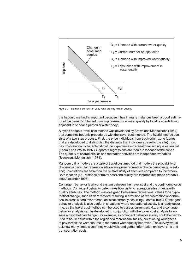
To compare visitation at sites with varying water quality, data are pooled on visitationfrom several sites that differ in water quality but are similar in other attributes, such asactivities performed and quality of facilities. The per capita demand for visits to thedifferent recreation sites, taking into account the transportation costs and travel time,is compared to assess the changes in trips per year as water quality improves. Thedemand curves are overlaid to measure the changes in benefits with changes in waterquality. In figure 3, demand for recreation at two sites is compared. Line D1 is the de-mand curve for a site with poor water quality, and D2 is the demand curve for a site withhigher water quality. With a constant travel cost (TC), the number of trips increasesfrom T1 to T2. The shaded region is the change in consumer surplus with a change inwater quality at similar sites.

Hedonic pricing techniques have been used in various applications to estimate pricesof nonmarket amenities that may be capitalized in the price of a housing unit (Michaeland others 1996). These nonmarket amenities include a variety of attributes, such asearthquake risk and water quality. Hedonic property models have been applied tomeasure the effects of water quality on property prices. Differences in property valuescan be used to measure benefits from higher water quality or changes in water quality.To obtain a demand curve for water quality improvements from the hedonic technique,it is necessary to use the hedonic technique with multiple markets. The utility derivedfrom portions of a river that vary from poor to good water quality, owing to local patternsof dischargers, can be compared. Benefits obtained from improvements in water qualitycan then be estimated. Necessary information includes property values, structural andlocational characteristics, and appropriate measures of water quality.

It has been estimated that a decrease in water quality significantly depresses propertyprices surrounding a lake or river. Changes in the quality of water are likely to affect theenjoyment of households owning property on or near the shoreline (Freeman 1979).The value of the property reveals information about the benefits property owners receivefrom water quality improvements. However, as Freeman states, property values derivedfrom analysis of housing costs reflect benefits to property owners, but not to others.For some water bodies, nonresident use is substantial. Regardless of the limitations,

Figure 2—Travel cost method demand curve and consumer surplus.

CS

Travel cost

Trips per season

Trip c

ost

Q

5

the hedonic method is important because it has in many instances been a good estima-tor of the benefits obtained from improvements in water quality by local residents livingadjacent to or near a particular water body.

A hybrid hedonic travel cost method was developed by Brown and Mendelsohn (1984)that combines hedonic procedures with the travel cost method. The hybrid method con-sists of a two-step process. First, the price individuals from each origin zone (zonesthat are developed to distinguish the distance that individuals travel to the site) mustpay to obtain each characteristic of the experience or recreational activity is estimated(Loomis and Walsh 1997). Separate regressions are then run for each of the zones.The quantity of characteristics and recreation activities are independent variables(Brown and Mendelsohn 1984).

Random utility models are a type of travel cost method that models the probability ofchoosing a particular recreation site on any given recreation choice period (e.g., week-end). Predictions are based on the relative utility of each site compared to the others.Both location (i.e., distance or travel cost) and quality are factored into these probabili-ties (Alexander 1995).

Contingent behavior is a hybrid system between the travel cost and the contingent valuemethods. Contingent behavior determines how visits to recreation sites change withquality attributes. The method was designed to measure recreational values for a hypo-thetical change, such as dam removal resulting in provision of river recreation opportuni-ties, in areas where river recreation is not currently occurring (Loomis 1999). Contingentbehavior analysis is also useful in situations where recreational activity is already occur-ring, as the travel cost method can be used to assess current activity, and a contingentbehavior analysis can be developed in conjunction with the travel cost analysis to as-sess a hypothetical change. For example, a contingent behavior survey could be distrib-uted to households within the region of a recreational facility, questioning willingnessto pay to visit the water source to recreate if water quality improved. The survey wouldask how many times a year they would visit, and gather information on travel time andtransportation costs.

Figure 3—Demand curves for sites with varying water quality.

D1 = Demand with current water quality

T1 = Current number of trips taken

D2 = Demand with improved water quality

T2 = Trips taken with improvement in water quality

Trips per season

Trip c

ost

D1 D2

T1 T2

Change in consumer surplus

6

The six water uses examined in this paper are municipal, industrial, hydropower,recreation, agricultural, and passive use, or instream flow. The U.S. Geological Survey(USGS) has estimated the Nation’s water use since 1950, from groundwater, freshsurface water, and saline surface water. Brown (1999) chose six water use categoriesfrom the USGS data to report national water demand: (1) livestock; (2) domestic andpublic; (3) industrial, commercial, and mining; (4) thermoelectric; (5) irrigation; and(6) hydroelectric power. We chose the former categories as they more closely followthe valuation literature.

As there are many different uses of water, it is not possible to come up with a singledefinition of water quality. Each water use has optimal water quality requirements thatare often unique. For example, municipal water, used for drinking and bathing, requireslow sediment levels. Water quality requirements for instream recreation depend on theactivity. Boating does not require a low sediment level, but swimming does. Peoplewho engage in rafting are more concerned with water quantity. Fish require particulartemperatures, and water quantity is important for recreational fishing. Water quality ismeasured by using some combination of water quality parameters. The parameters ofwater quality we will discuss are total suspended solids, dissolved oxygen, tempera-ture, salinity, clarity, and quantity.

We will define each of the water quality parameters and discuss the importance of eachone. We will then relate the parameters to the individual water uses. This discussionwill enable us to discuss how to value water quality improvements.

Water with a low amount of suspended solids is important to many water uses. Al-though amount of total suspended solids is important for recreational uses, the degreeof importance depends on the activity. For instance, swimming requires a low amount ofsuspended solids, whereas many of the rivers famous for whitewater rafting such as theColorado River, have a high sediment load. This does not mean that the level of totalsuspended solids is not important in rafting; it is just less important than for swimming.

Total suspended solids is measured as dry weight of particulates. Both organic andinorganic materials contribute to total suspended solids. Suspended solids can affectthe aquatic environment and its organisms by damaging macroinvertebrate communitiesthrough deposition, by reducing the abundance of food for fish, by directly affecting fishgrowth and resistance to disease, and by reducing the areas available for spawning andinterfering with fish egg and larval development (Hach Company 2001). Furthermore, thedeposition of organic matter can remove dissolved oxygen, an important element inhigh-quality water. A major source of total suspended solids in natural waters is runofffrom urban and agricultural areas.

Dissolved oxygen, gaseous oxygen (O2) dissolved in an aqueous solution, is an im-portant indicator of water quality. Oxygen is necessary to all aerobic forms of life,which provide stream purification. Dissolved oxygen is critical for fish and other waterinhabitants. Generally, waters with dissolved oxygen concentrations of 5.0 milligramsper liter (mg/L) (equivalent to 5 parts per million (ppm))1 or higher can support a well-balanced, healthy biological community. Some species, however, cannot tolerate even

Total Suspended Solids

Dissolved Oxygen

Water QualityParameters

1 One milligram per liter is the same as one part per million forwater solutions when the specific gravity of the solution is thesame as pure water under standard conditions. This is assumedto apply to low-concentration solutions.

7

slight depletion, and when concentrations fall below critical levels, the result is oftena complete alteration of the community structure. The consequences of changes indissolved oxygen frequently have both ecological and economic significance. Asdissolved oxygen drops below 5.0 mg/L, aquatic life is put under stress. The lowerthe concentration of oxygen, the greater the stress. Oxygen levels that remain below1 to 2 mg/L for a few hours can kill many fish. Note, however, that some systems with“good” water quality exhibit naturally low dissolved oxygen concentrations (e.g.,wetlands) (Hach Company 2001).

Nonmarket values and activities are dependent on adequate oxygen. Nonuse values,such as habitat quality, and use values, such as fishing, are uses of water for whichdissolved oxygen is an important parameter. A change in dissolved oxygen could causea decrease in fish catch, decreasing the quality of a fishing experience.

Water temperature is very important to many water uses. It affects chemical inter-actions and reactivity in the water column. Temperature also affects biological activity;many aquatic organisms have strict temperature requirements. The temperature ofwater in entire watersheds may become elevated by steam-electric generating plantsand other industries that use water to cool industrial processes (Gibbons 1986). If theheated water is discharged back into the stream, it disrupts the aquatic ecosystem,and damages fish habitat and wildlife. This practice is prohibited by the 1977 CleanWater Act and therefore is no longer seen as a threat to ecosystems. Cost of coolingthe water before disposal was about $10 per acre-foot in a study by Young and Gray(1972). Forest activities that can affect water temperature include overstory removal,enhancement of riparian vegetation, and revegetation activities. Removal of riparianvegetation is commonly believed to increase water temperature, but in particular circum-stances can allow for water temperature reductions. Activities that change streamconfiguration also can affect water temperature, such as structures or vegetation thatreduce channel width and increase channel depth and water velocity.

A river most often increases in salinity by flowing over salt deposits or picking upnonpoint agricultural runoff high in salt content. Removing salts from watersheds isan expensive process. Almost all water uses are adversely affected by salinity. It isestimated that every 1-ppm increase in salinity causes $230,000 worth of damage foragricultural, municipal, and industrial users (Gibbons 1986) in reduced crop yields anddamaged appliances and industrial machinery (Kleinman and Brown 1980). Thus, thebenefit of decreasing water salinity may outweigh the cost.

Water clarity is not generally termed pollution, so the importance of water clarity inbenefit measurement has to do primarily with aesthetics. Water clarity also determinesthe depth of light penetration and thereby the structure of habitats at various depths.Water clarity has both nonmarket and recreational use values.

The quantity of water is important in many water uses, such as healthy habitats andrecreation opportunities. Water quantity can either be too high or too low dependingon the use. Water quantity is often a contributing factor to all the parameters of waterquality previously mentioned. For example, as the quantity of water decreases, tem-perature may increase. On the other hand, as water quantity increases, salinity levelscan decrease per unit of water. Aside from the relations of other parameters to waterquantity, quantity alone is important to many uses. Daubert and others (1979) reported

Temperature

Water Clarity

Water Quantity

Salinity

8

a quadratic relation between water quantity and fishing benefits. They studied the valueof fishing, shoreline recreation, and whitewater activities in the Cache la Poudre River,Colorado, during summer 1978. At moderate flows, recreational fishing value was higherthan at higher flows. This may not be the case in boating, where value may increasewith increasing flows up to a point.

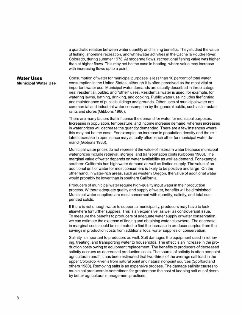
Consumption of water for municipal purposes is less than 10 percent of total waterconsumption in the United States, although it is often perceived as the most vital orimportant water use. Municipal water demands are usually described in three catego-ries: residential, public, and “other” uses. Residential water is used, for example, forwatering lawns, bathing, drinking, and cooking. Public water use includes firefightingand maintenance of public buildings and grounds. Other uses of municipal water arecommercial and industrial water consumption by the general public, such as in restau-rants and stores (Gibbons 1986).

There are many factors that influence the demand for water for municipal purposes.Increases in population, temperature, and income increase demand, whereas increasesin water prices will decrease the quantity demanded. There are a few instances wherethis may not be the case. For example, an increase in population density and the re-lated decrease in open space may actually offset each other for municipal water de-mand (Gibbons 1986).

Municipal water prices do not represent the value of instream water because municipalwater prices include retrieval, storage, and transportation costs (Gibbons 1986). Themarginal value of water depends on water availability as well as demand. For example,southern California has high water demand as well as limited supply. The value of anadditional unit of water for most consumers is likely to be positive and large. On theother hand, in water-rich areas, such as western Oregon, the value of additional waterwould probably be lower than in southern California.

Producers of municipal water require high-quality input water in their productionprocess. Without adequate quality and supply of water, benefits will be diminished.Municipal water suppliers are most concerned with quantity, salinity, and total sus-pended solids.

If there is not enough water to support a municipality, producers may have to lookelsewhere for further supplies. This is an expensive, as well as controversial issue.To measure the benefits to producers of adequate water supply or water conservation,we can estimate the expense of finding and obtaining water elsewhere. The decreasein marginal costs could be estimated to find the increase in producer surplus from thesavings in production costs from additional local water supplies or conservation.

Salinity is important to producers as well. Salt damages the equipment used in retriev-ing, treating, and transporting water to households. The effect is an increase in the pro-duction costs owing to equipment replacement. The benefits to producers of decreasedsalinity accrues as decreased production costs. The source of salinity is often nonpointagricultural runoff. It has been estimated that two-thirds of the average salt load in theupper Colorado River is from natural point and natural nonpoint sources (Spofford andothers 1980). Removing salts is an expensive process. The damage salinity causes tomunicipal producers is sometimes far greater than the cost of keeping salt out of riversby better agricultural management practices.

Water UsesMunicipal Water Use

9

Total suspended solids are important to municipal water producers. Total suspendedsolids are directly related to the treatment procedures that the supplier must use toensure safety. Ribaudo and Hellerstein (1992) describe the process of treating sourcewater for multiple uses by conventional methods such as filtration and disinfection.Water with low levels of total suspended solids may be treated by filtration, which elimi-nates the need for other treatments such as sedimentation. Cost savings for municipalwater producers when water has low total suspended solids accrue from the reducedneed for expensive and involved water treatment. Low turbidity levels also simplify thedisinfection process, thus making it less costly.

Agriculture is the major source of sediment in many parts of the country. Soil conserva-tion has a direct link to sediment load. Changes in municipal water production costsinduced by changes in sedimentation are a measure of the welfare effects accrued byproducers. It is simpler to estimate the benefits to producers than to consumers be-cause changes in producer surplus are measured by changes in production costs orprofits. Ribaudo and Hellerstein (1992) state that inputs and outputs of the water pro-duction process are generally priced in the market, and it is generally assumed thatthe production process is efficient.

Consumers of municipal water supplies are most concerned with four parameters ofwater quality: salinity, total suspended solids, water quantity, and clarity. Irrigation offarmland has been shown to be a factor in salinity in the Colorado River basin, andelsewhere. High salinity can damage water-using appliances and pipes, increase theuse of detergents, and deteriorate clothing and other textiles (Ribaudo and Hellerstein1992). The benefits to consumers of decreased salinity come in the form of decreasedcosts of replacing appliances, pipes, clothing, and so on.

A common approach in the literature to estimate benefits to consumers from a decreasein salinity is to estimate physical damage in terms of expected appliance lifetimes, as-suming that the household would be willing to pay up to the economic value of thosephysical damages to avoid them (d’Arge and Eubanks 1978). The method uses regres-sion equations that relate appliance lifespan to salinity.

Total suspended solids create many of the same effects as salinity; however, totalsuspended solids are also related to health and safety of the public. Many outbreaksof infectious diseases have been traced to contaminants in municipal water supplies.A low amount of total suspended solids in the public water supply is an importantnonmarket benefit of improved water quality.

Directly estimating household demand or expenditure functions for water quality is gen-erally not possible, as households cannot directly purchase water of varying quality(Ribaudo and Hellerstein 1992). It is still important to measure the benefits consumersgain from knowing their water is of high quality and is treated with the best availabletechnology to ensure safety. To measure the benefits of increased drinking water quality,we look at people’s willingness to pay for improvements in water quality. The contingentvaluation method can be used to measure willingness to pay for improvements in waterquality. Contingent valuation is a flexible tool as it allows the measurement of benefits ofchanges in an environmental good not traded in a formal market (Jordan and Elnagheeb1993). To examine the benefit of improving residential water quality, a contingent valua-tion survey would describe the current state of water quality and then create a hypotheti-cal situation of an improvement in water quality. The description should be realistic andprecise enough to give the respondent adequate information on which to base a valua-tion (Loomis and Walsh 1997).

10

Table 1 summarizes two studies, each using the hedonic property method, concerningchanges in property prices near water bodies given a change in water clarity. Thestudies examined the change in property price for each foot of lake frontage given a1-foot improvement in water clarity. In addition to these studies, Feather (1992) foundchanges in the parcel price of land resulting from decreases in water clarity, by usingthe hedonic method in Orange County, Florida. The value is unique for each situation,such as location and current clarity.

Scarcity of water increases its marginal value. However, when water quantity is ad-equate to satisfy demand, total benefits to consumers increase. Table 2 summarizesthree studies concerning water values to municipal water users given a change in waterquantity. Values were found for a 10-percent reduction in quantity supplied and wereexpressed in terms of dollars per acre-foot. The range of values demonstrates theimportance of clearly defining what is being valued. In these cases, water quantitychanges for general municipal use, for lawns, and for indoor domestic use had verydifferent values.

Table 1—Increase in property value per foot of lake frontage for 1-footimprovement in water clarity

ValuationCitation method Location Value

1998 U.S. dollarsMichael and others 1996 Hedonic China Lake, Maine 28.00Michael and others 1996 Hedonic Cobbossee Lake, Maine 16.37Michael and others 1996 Hedonic Long Lake, Maine 17.53Steinnes 1992 Hedonic Northern Minnesota 2.34

Table 2—Value of water for municipal use

Value per Type ofCitation Valuation method Location acre-foot value

1998U.S. dollars

Danielson 1977 Value of a 10-percent South Atlantic 41.02 Summerquantity reduction Gulf

Danielson 1977 Value of a 10-percent South Atlantic 41.02 Winterquantity reduction Gulf

Young 1973 Value of a 10-percent Lower Colorado 351.08 Summerquantity reduction

Young 1973 Value of a 10-percent Lower Colorado 54.32 Winterquantity reduction

Young and Indeterminate Unspecified 359.17 Domestic lawnGray 1972 watering

Young and Indeterminate Unspecified 653.21 Indoor domesticGray 1972 use

11

Table 3—Value for municipal water use of water quality improvement

Annual householdCitation Location value per 1 mg/La Cost and benefit

improvement

1998 U.S. dollarsKleinman and Colorado River, CO 0.0469 Mean cost from previous studies,

Brown 1980 decrease in salinity and totalsuspended solids

Ragan and Arkansas River .0533 Benefit from a decrease in salinityothers 1993 watershed, CO from 500 mg/L to 200 mg/L

Ragan and Arkansas River .0365 Benefit from a decrease in salinityothers 1993 watershed, CO from 1,000 mg/L to 200 mg/L

Ragan and Arkansas River .0280 Benefit from a decrease in salinityothers 1 993 watershed, CO from 1,500 mg/L to 200 mg/L

Ragan and Arkansas River .0235 Benefit from a decrease in salinityothers 1993 watershed, CO from 2,000 mg/L to 200 mg/L

Ragan and Arkansas River .0193 Benefit from a decrease in salinityothers 1993 watershed, CO from 3,000 mg/L to 200 mg/L

Ragan and Arkansas River .0177 Benefit from a decrease in salinityothers 1993 watershed, CO from 4,000 mg/L to 200 mg/L

Ragan and Arkansas River .0264 Benefit from a decrease in salinityothers 1993 watershed, CO from 1,000 mg/L to 500 mg/L

Ragan and Arkansas River .0176 Benefit from a decrease in salinityothers 1993 watershed, CO from 2,000 mg/L to 500 mg/L

Ragan and Arkansas River .0152 Benefit from a decrease in salinityothers 1993 watershed, CO from 3,000 mg/L to 500 mg/L

Ragan and Arkansas River .1480 Benefit from a decrease in salinityothers 1993 watershed, CO from 4,000 mg/L to 500 mg/L

a Milligrams per liter.

Table 3 provides information from Kleinman and Brown (1980) and Ragan and others(1993) concerning total suspended solids and salinity in municipal water uses. Bothstudies used a cost savings valuation method to assess the impact of salinity and totalsuspended solids on municipal users. Salinity and total suspended solids were com-bined because they cause similar damages, such as to appliances and clothes. Raganand others (1993) outline annual benefits to households for a decrease in salinity to200 mg/L or 500 mg/L. The study results show that the marginal value for each milli-gram per liter decrease is less for higher initial salinity.

Water quality affects agricultural uses of water in many ways. Agriculture is also asource of water quality issues. Runoff and return flows from irrigated fields carry dis-solved salts leached from the soil. As river flow is diverted for irrigation, the concentra-tion of total dissolved solids increases, reducing the productivity of the water foragriculture (Freeman 1979). Irrigation of land is a primary water use by agricultural

Agricultural Water Use

12

producers, and without proper water quality, decreased crop production and diseasemay result. There are various ways benefits gained from an improvement in water qual-ity for agricultural purposes can be measured, both to consumers and producers.

To the extent that water quality affects agricultural productivity, it can affect the cost ofproduction for a variety of goods and services (Freeman 1979). Water quality is a factorin the production function of an agricultural good. To measure the benefits gained froma water quality improvement, changes in market variables involved in production of thegood are evaluated. Benefits from a change in water quality are felt in two ways: throughchanges in price to consumers, and through changes in the incomes received by own-ers of inputs used in the production of the good (Freeman 1979).

Salinity, total suspended solids, available water quantity, and water temperature are thewater parameters agricultural producers are most concerned with. The measurement ofbenefits to agricultural producers is similar to that of producers of municipal water. Thesignificant difference is that quantity can change; for municipal water, output quantityremained constant, so consumer surplus did not change and the cost of productionchanged only producer benefits.

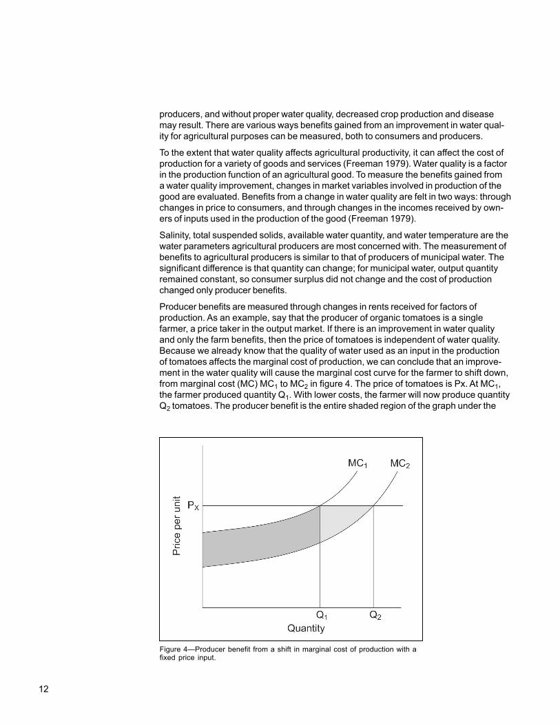
Producer benefits are measured through changes in rents received for factors ofproduction. As an example, say that the producer of organic tomatoes is a singlefarmer, a price taker in the output market. If there is an improvement in water qualityand only the farm benefits, then the price of tomatoes is independent of water quality.Because we already know that the quality of water used as an input in the productionof tomatoes affects the marginal cost of production, we can conclude that an improve-ment in the water quality will cause the marginal cost curve for the farmer to shift down,from marginal cost (MC) MC1 to MC2 in figure 4. The price of tomatoes is Px. At MC1,the farmer produced quantity Q1. With lower costs, the farmer will now produce quantityQ2 tomatoes. The producer benefit is the entire shaded region of the graph under the

Figure 4—Producer benefit from a shift in marginal cost of production with afixed price input.

13

constant price Px. The dark area is the benefit from the reduction of costs to producethe original amount of tomatoes, Q1. The lighter-shaded area represents the benefitsreceived from the inframarginal rent on the increase in output. Inframarginal rent is aterm used to describe the producer surplus earned on all units of production but thelast one.

Agricultural consumers are concerned with the same water quality parameters thatconcern producers. Assuming a change in production costs will result in a change inthe output price, there will be a change in consumer surplus in addition to the changein producer surplus. As can be seen in figure 5, when demand DQ is elastic and themarginal cost of production changes from MC1 to MC2, the total benefit to both consum-ers and producers is equal to the net change in the sum of the surpluses, or the entireshaded region. Because most agricultural products are traded in national and interna-tional markets, it is rare that a change in water quality in one watershed would haveany effect on the price of most agricultural products. The exception would be locallygrown and consumed specialty crops (Freeman 1979).

Figure 5—Producer and consumer surplus from a shift in marginal cost ofproduction with elastic demand.

Water quantity is an important concern to agricultural producers. Table 4 summarizesfive studies concerning the benefits to agricultural producers given an increase inwater. The primary method used is to measure the change in production costs givena 1-acre-foot change in water availability. The study areas were the Pacific Northwest,Idaho, and Montana. Again, the variation in water value emphasizes that value is afunction of use.

Quantity

Pric

e pe

r un

it

MC2MC1

Q2Q1

P2

P1

14

Figure 6—Value of damages to agriculture owing to total suspended solids and salinity.

Table 4—Value of water for agriculture

Value perCitation Valuation method Location acre-foot Crop

1998 U.S. dollars

Aillery and others 1994 Change in production costs Pacific Northwest 34.36

Ayer 1983 Change in production costs Washington 202.94

Ayer and others 1983 Change in production costs Idaho 597.77

Washington State University 1972 Farm crop budget Yakima River basin, WA 20.46 Cotton

Washington State University 1972 Farm crop budget Yakima River basin, WA 171.68 Melons

Washington State University 1972 Farm crop budget Yakima River basin, WA 62.53 Melons

Washington State University 1972 Farm crop budget Yakima River basin, WA 20.71 Potatoes

Washington State University 1972 Farm crop budget Yakima River basin, WA 155.76 Safflower

Washington State University 1972 Farm crop budget Yakima River basin, WA 103.46 Safflower

Duffield and others 1992 Change in production costs Bitterroot, MT 55.71

Duffield and others 1992 Change in production costs Big Hole, MT 26.15

Figure 6 illustrates changes in benefits to agricultural producers given a change insalinity or total suspended solids, from Kleinman and Brown (1980). They estimateforgone production minus direct variable costs to agricultural producers relying onwater in the lower mainstem of the Colorado River. Salinity and suspended solidswere combined because of the nature of damages that they cause. There is anincrease in damages as the milligrams of suspended solids per liter increases.

200

150

100

50

0

800

850

900

950

1,00

0

1,05

0

1,10

0

1,15

0

1,20

0

1,30

0

1,40

0

Suspended solids and salinity (milligrams per liter)

Annu

al v

alue

(199

8 do

llars

)

15

The demand for water-based recreation has been increasing as our population expandsand the desire for outdoor recreation grows, particularly near urban areas and in nationalparks and other unique sites. Although some rivers heavily used for recreation, and hold-ing other values as well, have been protected by legislation, there are still many water-sheds that have been altered by dams and waterway construction, or pollution.

Water-based recreation is affected by all the water quality parameters that we havediscussed. The relative importance of water quality parameters depends on the activity.Swimming requires higher quality water than boating. For waterskiing, users will prefera site where the sediment is low, but sediment may not be as detrimental for activitiessuch as whitewater rafting, where the main concern is an adequate water supply. Manyfamous whitewater rivers such as the Colorado have high sediment loads. To calculatethe benefits of water quality improvements, we must measure the value of water forthe particular recreational activity. There are various ways we can measure the addedbenefits people receive when the quality of their experience is improved, or when waterquality is improved. Although several recreation activities may respond to water qualityimprovement, the activities are not necessarily homogenous; they may responddifferently to changes in water quality.

Dissolved oxygen, total suspended solids, temperature, and water quantity are importantwater quality parameters for fish and, therefore, fishing. Sutherland (1982) states that thebenefits of improved water quality can be defined as net willingness to pay for waterquality improvement. Rafters are most concerned with water quantity. Rafters withdifferent skill levels often want different water quantities. The amount of total suspendedsolids is not as important to rafters as is water quantity; it is also not as important forrafting as for other uses, such as swimming and fishing. Water quality also is importantfor the many recreational activities associated with water shorelines, such as viewingwildlife and camping. Parameters important to shoreline activities include water clarity,total suspended solids, and water quantity.

We can use the same nonmarket valuation methods to find the benefits of improvedwater quality for various recreationists, such as shoreline recreationists and rafters,although the results may be quite different. For example, water must have low amountsof total suspended solids to be classified as swimmable. The value of a decrease of totalsuspended solids may be higher for swimming than for rafting or boating. Daubert andothers (1979) conducted a survey to determine the marginal values of different stream-flows in the Cache la Poudre River in Colorado for fishing, shoreline recreation, andwhitewater activities. Recreationists were asked what they would be willing to pay tohave more water. Depending on the activity, marginal values could be positive if morewater resulted in higher utility, or negative if more water resulted in decreased utility. Thehighest marginal value for fishing, $16 (in 1980 dollars) per acre-foot, was found with lowflows (50 to 90 cubic feet per second); water value dropped to zero as flows reached450 to 500 cubic feet per second. For shoreline recreation, the maximum marginal valuealso occurred at low flows and was $11 per acre-foot, falling to zero at flows of 700 to750 cubic feet per second. The value for whitewater recreation exhibited constantmarginal returns of $6 per acre-foot at the range of flows in the survey.

Recreation Use

16

Table 5—Value of water quality improvements for recreation (decrease in total suspended solids and salinity)

Citation Valuation method Location Value Water use change

1998 U.S. dollarsMean increase in benefit per household

Carson and Mitchell 1993 Contingent valuation National 104.29 Nonboatableto boatable

Carson and Mitchell 1993 Contingent valuation National 79.60 Boatable tofishable

Carson and Mitchell 1993 Contingent valuation National 88.68 Fishable toswimmable

Smith and others 1986 Contingent valuation Monongahela River, PA 35.65 Loss of areaSmith and others 1986 Travel cost Monongahela River, PA 6.38 Loss of areaSmith and others 1986 Contingent valuation Monongahela River, PA 38.31 Boatable to

game fishingSmith and others 1986 Travel cost Monongahela River, PA 12.95 Boatable to

game fishingSmith and others 1986 Contingent valuation Monongahela River, PA 56.39 Boatable to

swimmableSmith and others 1986 Travel cost Monongahela River, PA 52.20 Boatable to

swimmableMean annual recreation benefits

Activity:Sutherland 1982 Travel cost 119 counties of ID, OR, and WA 54,630 SwimmingSutherland 1982 Travel cost 119 counties of ID, OR, and WA 48,957 CampingSutherland 1982 Travel cost 119 counties of ID, OR, and WA 98,303 FishingSutherland 1982 Travel cost 119 counties of ID, OR, and WA 66,515 Boating

Table 5 provides information about the increase in benefits to recreationists given animprovement in water quality. Values were estimated by using contingent valuation andtravel cost methods. Fishing provided the greatest annual benefits in the Pacific North-west, whereas camping provided the least, reflecting the importance of water quality toeach activity.

Table 6 provides detail from Smith and Desvousges (1986), who estimated recreationvalues for changes in water quality. The travel cost method was used to find benefitsper trip for changes in water quality. The sites were primarily in the Midwest, South,and Southeast. They estimated two values for water quality, one for water suitable forboating and fishing, and one for water suitable for boating and swimming.

Table 7 summarizes nine studies that use the contingent valuation and travel costmethods to assess the benefits to recreationists given an increase in water quantity.Various locations and activities are included in the table to illustrate the variabilityacross sites and activities. The marginal value depends on the site and the activitiesdone at each site.

17

Table 6—Recreational benefits measured by the travel cost method for a changein dissolved oxygen saturation of 1 percent

Value of improvement per trip

Location Boatable Fishable 1998 U.S. dollars

Arkabutla Lake, MS 4.09 4.59Lock and Dam 2, Arkansas River navigation system, AR 4.04 4.67Belton Lake, TX 1.35 1.48Benbrook Lake, TX .55 1.00Blakely Mt. Dam, Lake Ouachita, AR .47 .53Canton Lake, OK .69 .74Cordell Hull Dam and Reservoir, TN 1.98 2.19Defray Lake, AR 1.48 1.58Grapevine Lake, TX .53 .58Grenada Lake, MS 2.67 3.03Hords Creek Lake, TX .42 .47Melvern Lakes, KS .77 .84Millwood Lake, AR 4.70 5.15Mississippi River pool 6, MN .05 .05New Savannah Bluff Lock and Dam, GA 1.82 2.06Ozark Lake, AR .87 .98Philpott Lake, VA 2.32 2.61Proctor Lake, TX .11 .13Sam Rayburn Dam and Reservoir, TX 1.29 1.42Sardis Lake, MS 1.27 1.42Whitney Lake, TX .95 1.06

Source: Smith and Desvousges 1986.

Because there are 17 different value estimates for instream flow values in table 7, itis possible to perform a systematic, quantitative analysis for relations by using meta-analysis. Meta-analysis is a commonly used quantitative reversion technique appliedto evaluate results of past studies for patterns or consistency of findings. The studiessummarized in table 7 were examined by using meta-analysis to determine what, if any,statistical relation might exist between the value per acre-foot increase, and indepen-dent variables that include waterflow, recreational activity, and valuation method used.Results of the regression are outlined in table 8. The functional linear form between thevariables resulted in the best t-statistics, and highest explanatory power at 59 percent.

Water Quantityand RecreationMeta-Analysis

18

Table 7— Value of water for recreation uses

Additional Marginal value feet per

Citation method Valuation method Location per acre-foot second Type of activity

1998 U.S. dollarsDaubert and Young 1981 Contingent valuation Poudre River, CO 14.50 100 FishingDaubert and Young 1981 Contingent valuation Poudre River, CO 13.44 100 RaftingDaubert and Young 1981 Contingent valuation Poudre River, CO 14.50 100 ShorelineWalsh and others 1980 Contingent valuation West Slope Rivers, CO 6.94 1,400 KayakingWalsh and others 1980 Contingent valuation West Slope Rivers, CO 4.50 2,800 RaftingWalsh and others 1980 Contingent valuation West Slope Rivers, CO 24.46 1,120 FishingWard 1987 Travel cost Rio Chama, NM 40.32 1,000 Rafting and fishingHarpman 1990 Contingent valuation Taylor River, CO 3.10 40 FishingDuffield and others 1992 Contingent valuation Big Hole, MT 34.12 100 FishingDuffield and others 1992 Contingent valuation Bitterroot, MT 13.44 100 Fishing and shorelineJohnson and Adams 1988 Contingent valuation John Day River, OR 3.10 204 FishingLoomis and Creel 1992 Travel cost San Joaquin, CA 90.00 2,000 Fishing and otherLoomis and Creel 1992 Travel cost Stanislaus, CA 16.54 300 Fishing and otherLoomis and Cooper 1990 Travel cost North Fork Feather, CA 91.63 20 FishingLoomis and Cooper 1990 Travel cost North Fork Feather, CA 71.29 100 FishingLoomis and Cooper 1990 Travel cost North Fork Feather, CA 57.44 200 FishingLoomis and Feldman 1995 Contingent valuation Snake River, ID 76.00 235 Viewing of falls

Table 8—Linear and double log meta-analysis regression results for marginalbenefits from an increase in streamflowa

Linear: CFSb

Dependent Log-log:Form variable Constant Valmethod Fish Boat LNCFSc F-stat R2

Linear VAFd 40.88 50.42 -26.53 -35.84 0 .004 4.37 .59

(2.82)e (3.69) (-1.56) (-1.99) (.48)

Log-Log LNVAFf 3.13 1.76 -0.84 -1.04 .02 3.30 .52

(2.90) (3.28) (-1.26) (-1.48) (.09)

a Number of observations = 17 with 12 degrees of freedom. Studies are outlined in table 7.b CFS = water flow in cubic feet per second.c LNCFS = log of CFS.d VAF = value per acre-foot increase.e Numbers in parentheses are t statistics.f LNVAF = log of VAF.

19

The estimation resulted in the following equation:

VAF = ß0 + ß1valmethod - ß2fish - ß3boat + ß4CFS

where VAF is the value per acre-foot increase in 1998 dollars,

valmethod is a dummy variable for the valuation method used where 0 = contingent valuation and 1 = travel cost,

fish is a dummy variable for fishing where fishing = 1 and not fishing = 0,

boat is a dummy variable for boating where boating = 1 and not boating = 0, and

CFS is waterflow in cubic feet per second.

In the log-log equation, LNVAF is the log of the value per acre-foot increase in flow, andLNCFS is the log of waterflow in cubic feet per second.

The overall linear regression does a good job explaining nearly 60 percent of the variationin values for instream flow. The coefficient on valmethod indicates that if the travel costmethod was used, then the marginal value per acre-foot increases by $50.42, ascompared to a contingent valuation method study. The t-statistic is significant at the1-percent level. If the activity performed is boating, the marginal value per acre-footdecreases by $35.84. The t-statistic for this variable is significant at the 5-percentlevel. The variable CFS has a low t-statistic, indicating waterflow is not significant inthe model. This suggests that the recreational value of instream flow appears not tobe related to the absolute flow level. It may be that relative flow concepts, such aspercentage bankfull elevation2, used in the Walsh and others (1980) analysis is a moremeaningful concept when comparing waterflows across rivers and studies. As additionalinstream flow studies become available, this analysis could be updated to improve themeta-analysis. An improved meta-analysis equation could be used to provide a simplebenefit-transfer for providing rough estimates of the value of instream flow on rivers withoutexisting studies.

Industrial water use in the United States accounts for approximately 43 percent of with-drawals and 9 percent of consumption (U.S. Water Resources Council 1978). Industrialwater use is water used as an input in a production process, such as cooling, conden-sation, washing, and moving materials (Gibbons 1986). Water may also be incorporatedinto products.

Industrial intake water must meet various water quality standards. Industrial users ofwater are concerned with total suspended solids, salinity, and quantity of water avail-able. Depending on the use, quality standards differ in stringency. If the water is usedfor human consumption or for boiler feed, quality requirements are the most stringent.

2 Bankfull elevation is the elevation of the depositional flat,immediately adjacent to the channel (Leopold 1994). Thestreamflow most effective in producing and carrying sedimentis the flow at bankfull elevation (Verry 2000). Bankfull is thatportion of the channelway usually defined by a topographicbreak, where water would completely fill the channel to thelevel of the adjacent floodplain. It represents a common referencepoint for measuring flows (personal communication, April 2002,Dr. Gordon Grant, research hydrologist, USDA Forest Service,Pacific Northwest Research Station, Forestry Sciences Lab,3200 SW Jefferson Way, Corvallis, OR 97331).

Industrial Water Use

20

High salinity or suspended solids could be detrimental to equipment (Gibbons 1986).The quantity of water available is also important. Many companies have their own wellsfor general process water supply.

Like some agricultural and municipal water uses, industrial water use can result inwater quality degradation. The cooling process carries away waste heat, raising watertemperature if discharged back to the water source. Evaporative losses may increasethe concentration of salts. Chemical and petroleum refining may introduce organicchemicals and solvents into the effluent (Kleinman and Brown 1980).

Changes in marginal costs of production must be estimated to calculate the changein benefits to industrial producers from improvements in water quality. In most cases,if total suspended solids or salinity decreases in the input water, there is a decreasein production costs, for example, by eliminating certain treatments or in longer equip-ment life. These changes in benefits are measured by deriving a new marginal costcurve given the decrease in production costs. The increase in producer surplus is thenmeasured for production of the same amount of the good, given that the price to theconsumer remains constant and only the producers benefit. This is the same methodused for agricultural producers given that the price of the good remains constant.

Assuming the price of a good changes with a change in marginal cost of production,we would expect to see an increase in consumer benefits given improvements in waterquality. The methods for measuring the increase in consumer surplus are the same asdescribed for agricultural products.

Table 9 summarizes four studies concerning the values of water for industrial uses.Water value was calculated in most of the studies by examining changes in productioncosts for a particular industry. The values are highly variable between industries. Forexample, the value per acre-foot of water for the chemicals industry is $99, while thelow estimate for the meat packing industry is $637 per acre-foot. The meat packingindustry may require more water of higher quality in their production processes thandoes the chemical industry.

Heintz and others (1976) and Unger (1978) provide estimates of annual damages thatindustries face because of poor water quality owing to salinity and suspended solids.Heintz and others (1976) estimated total annual damages at $968 million, and Unger(1978) at $1.9 billion, in 1998 dollars. There is little information on benefits for industrialwater use owing to the uniqueness of industrial uses, and differences in damage esti-mates are due to variations in industry uses.

Hydropower has been a source of energy for many years, for activities such as the useof water wheels to rotate grindstones for milling wheat, corn, and other grains. In 1980,the United States relied on hydropower from dams for about 12.1 percent of the powerconsumed in the country. Hydropower is an important method of obtaining energy andhas many advantages. One unit of water generates hydropower cumulatively by passingthrough turbines of many dams along the descent of a river (Gibbons 1986). Hydropowerproduces less pollution than the extraction and burning of fossil fuels such as coal ornatural gas.

Hydropower does have disadvantages. Depending on their construction, dams caneventually silt in or wear out. Dams cause the inundation of vast amounts of land,destruction of fish and wildlife habitat, and the loss of whitewater recreational

Hydropower Water Uses

21

opportunities (Gibbons 1986). Dams also may cause changes in water temperature.Decreased movement of sediment through the system contributes to loss of habitatand recreational opportunities downstream. These effects are cumulative in a systemof dams.

Parameters most important for hydropower production are water quantity and salinity.Salinity affects hydropower production in some of the same ways it affects industrialproduction. If salinity is too high, penstocks and turbines may deteriorate more quickly.Measurement of benefit from improvements in salinity levels is estimated by determiningthe increase in equipment lifespans and savings in replacement costs. Water quantityis important in hydropower production. Without an adequate water supply, efficiency islowered. When valuing water for hydropower, it is important to note that the productivityfor hydropower is constant. Each acre-foot of water dropped over a given head (verticalfeet) makes the same amount of electricity, so the marginal and average productivitiesof water in this use are equal. On a specific river, the amount of electricity produced perunit of water is a function of both the average net head on the river and the conversionefficiency of the particular hydropower facility (specifically, the efficiency of the conver-sion of the energy of falling water into electrical energy) (Gibbons 1986). This relation isfairly standard and can be expressed as 0.87 kilowatt per acre-foot of head (Whittleseyand others 1981).

As water quantity increases in a river, we would expect to see an increase in hydro-power production and an increase in revenues. The increase in revenue can be calcu-lated by multiplying the acre-feet of water by 0.87 times the value of a kilowatt-hour.However, there must be a demand for the power when the water is available. At highspring flows, electricity demand for heating and cooling is low, so a lower price maybe received.

Table 9—Values of water for industrial use

Valuation Value per Type ofCitation method acre-foot industry

1998 U.S. dollars

Young and Gray 1972 Indeterminate 99.77 Chemical industry

Young and Gray 1972 Indeterminate 125.27 Paper manufacturing

Young and Gray 1972 Indeterminate 31.04 Minerals industry

Russell 1970 Change in 146.33 Beet sugar processingproduction costs

Kollar and others 1976 Change in 259.40 Cotton textile finishingproduction costs

Kane and Ostantowski Change in 637.42 Low estimate,meat1980 production costs packing industry

Kane and Ostantowski Change in 889.07 High estimate, meat1980 production costs packing industry

22

Consumers of hydropower obtain benefits when water quantity increases. With an in-crease in waterflow, there is a potential increase in kilowatt-hours produced. This resultsin a lower marginal cost curve to producers because they are now able to provide moreelectricity. As demand for electricity is usually inelastic, consumers of electricity obtainbenefits from water quantity increases in the form of decreased prices.

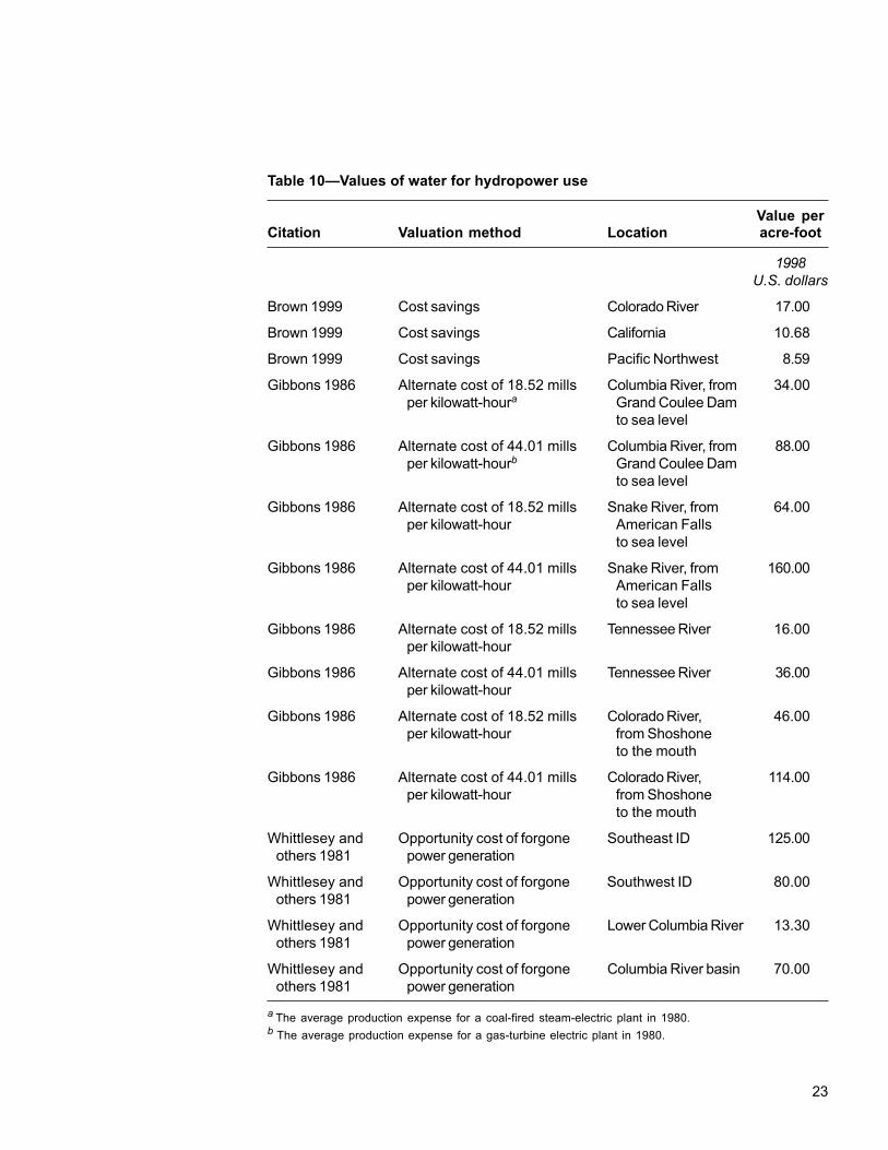
Table 10 summarizes information from three studies concerning the values of water forhydropower use. The hydropower industry relies on a large supply of water to provideenergy to their customers. The cost savings of hydropower compared to other means ofproducing electricity were found for different parts of the country by Brown (2000). Alter-nate costs of firm and peak levels of production were found for other means of providingelectricity for certain parts of the country and then compared to the same productionlevel from hydropower by Gibbons (1986). Whittlesey and others (1981) evaluated theopportunity cost of forgone power production owing to agricultural diversions.

Nonmarket values for water include onsite use value and nonuser benefits. Nonuserbenefits of water include benefits people obtain without making direct use of water, suchas ecological value, preservation benefits, and option or bequest values. These benefitsare hard to measure because they are often not linked to observable behavior. Param-eters necessary in defining water quality for nonuse benefits may include clarity, quan-tity, total suspended solids, salinity, dissolved oxygen, and temperature.

Many people receive value from high water clarity because they own or visit land nearwater bodies and clarity affects aesthetics. Water quality must be sustainable to ensurethe environmental quality of particular ecosystems, as high levels of suspended solidsor salinity can be harmful to aquatic ecosystems. Spawning areas, food sources, andhabitats can be harmed, and there can be direct damage to fish, crustaceans, andother aquatic wildlife (Clark and others 1985). Many upstream activities can causesmall changes in water temperature, and results can potentially be devastating. Manyaquatic organisms have strict temperature requirements and thus are susceptible tofluctuations in temperature. Dissolved oxygen is extremely important for the survival ofmany species. If the amount of dissolved oxygen is disrupted, there can be a seriousalteration of the aquatic ecosystem. However, some systems are defined as having goodwater quality even if their dissolved oxygen concentrations are low, such as wetlands;different water bodies have different uses, and acceptable water quality will depend onthese uses. Alterations of the parameters can be detrimental to fish and wildlife in manyecosystems.

Water quantity is an important parameter for many habitats. It has been shown thatthe marginal value of instream flow for fish habitat gradually drops as flows reach amaximum (Brown 1991). Low streamflow can cause concentrations of many pollutantsto increase, and cause an increase in water temperature.

Lakefront properties can be viewed as heterogeneous goods; they have many differentcharacteristics and are differentiated from each other by the quality and quantity ofthese characteristics (Michael and others 1996). When consumers purchase differenti-ated goods, they are purchasing the characteristics that make up that good (Lancaster1966). If the quality of any of the characteristics of the goods changes, we would expectthe price of the good to change. If the quality of water surrounding lakefront propertyimproves, we expect the price of the property to increase because water quality is acharacteristic of the property. The hedonic valuation method allows the measurementof benefits of water quality through the price differences of housing.

Nonmarket andNonuse Values

23

Table 10—Values of water for hydropower use

Value perCitation Valuation method Location acre-foot

1998U.S. dollars

Brown 1999 Cost savings Colorado River 17.00

Brown 1999 Cost savings California 10.68

Brown 1999 Cost savings Pacific Northwest 8.59

Gibbons 1986 Alternate cost of 18.52 mills Columbia River, from 34.00per kilowatt-houra Grand Coulee Dam

to sea level

Gibbons 1986 Alternate cost of 44.01 mills Columbia River, from 88.00per kilowatt-hourb Grand Coulee Dam

to sea level

Gibbons 1986 Alternate cost of 18.52 mills Snake River, from 64.00per kilowatt-hour American Falls

to sea level

Gibbons 1986 Alternate cost of 44.01 mills Snake River, from 160.00per kilowatt-hour American Falls

to sea level

Gibbons 1986 Alternate cost of 18.52 mills Tennessee River 16.00per kilowatt-hour

Gibbons 1986 Alternate cost of 44.01 mills Tennessee River 36.00per kilowatt-hour

Gibbons 1986 Alternate cost of 18.52 mills Colorado River, 46.00per kilowatt-hour from Shoshone

to the mouth

Gibbons 1986 Alternate cost of 44.01 mills Colorado River, 114.00per kilowatt-hour from Shoshone

to the mouth

Whittlesey and Opportunity cost of forgone Southeast ID 125.00others 1981 power generation

Whittlesey and Opportunity cost of forgone Southwest ID 80.00others 1981 power generation

Whittlesey and Opportunity cost of forgone Lower Columbia River 13.30others 1981 power generation

Whittlesey and Opportunity cost of forgone Columbia River basin 70.00others 1981 power generation

a The average production expense for a coal-fired steam-electric plant in 1980.b The average production expense for a gas-turbine electric plant in 1980.

24

Property attributes are also an important nonmarket benefit. Although property ownersmay not consume the water in a lake or stream, water adjacent to property has aes-thetic value and attracts wildlife, which residents enjoy. Property owners receive eco-nomic value from water clarity. In a study of lakefront property in Maine by Michael andothers (1996), house price per foot of lake frontage was modeled as a function of waterclarity at the time the property was purchased, along with other factors such as squarefootage and number of bedrooms. The study found that estimated increases in sellingprice of the average lakefront property owing to a 1-meter improvement in water clarityranged from $34 to $81 per foot of lake frontage, depending on the lake valued. Esti-mated decreases in the selling price of the average lakefront property owing to a 1-meterreduction in water clarity ranged from $65 to $141 per foot of lake frontage. Estimatesof the aggregate property price increase around an entire lake owing to a 1-meter waterclarity improvement ranged from $6,528,000 to $9,365,900, whereas estimates of theaggregate price decrease around an entire lake owing to a 1-meter reduction in waterclarity were between $12,480,000 and $16,080,700.

Loomis and others (2000) used contingent valuation to estimate values per acre-foot ofwater on the Platte River in Colorado at $771. Douglas and Taylor (1999) used contin-gent valuation to assess several scenarios on the Trinity River in California. They esti-mated values per acre-foot of water that ranged from $536 to $957. Table 11 illustratesthe value of salmon given changes in water quality. It is interesting to note that as thenumber of salmon assumed to exist in each study goes down, the marginal value persalmon increases, reflecting the increased scarcity.

In table 12, values for water quality for nonusers are outlined from three studies. In eachstudy, survey respondents are valuing improvements in water quality related to salinity,suspended solids, and water quantity.

Table 11—Nonmarket nonuse values of additional salmon owing to an increasein water quality

Number ofCitation Valuation method Location Value salmon

1998U.S. dollars

Loomis 1999 Contingent valuation Pacific Northwest 1,400 1,000,000and California

Loomis 1999 Contingent valuation Pacific Northwest 10,712 250,000and California

Olsen and others Contingent valuation Pacific Northwest 203 2,500,0001991 and California

Loomis 1996 Contingent valuation Pacific Northwest 3,325 300,000

Hanemann and Contingent valuation California 232,356 14,900others 1991

25

Table 12—Nonmarket values of water quality (salinity and total suspendedsolids) and quantity

Valuation Value perCitation method Location household Notes

1998 U.S. dollars

Greenley and Contingent South Platte 95.00 Existence and bequestothers 1981 valuation River basin values of nonrecreationists

from Fort Collins

Greenley and Contingent South Platte 99.00 Existence and bequestothers 1981 valuation River basin values of nonrecreationists

from Denver Metro and theSouth Platte basin

Loomis 1987 Contingent Mono Lake 131.00 Utility bill increase for firstvaluation level of improvement in

lake level, visibility, andbird survival and diversity

Heintz and Contingent Fraser River 656.00 Preservation value of salmonothers 1976 valuation valley

Conclusion Across the Nation, there are significant challenges to policymakers and decision-makers concerning the allocation of high-quality water to the many uses and users.The challenge is to manage federal lands to provide abundant, clean, high-qualitywater to sustain a burgeoning population, an agricultural industry, historical salmonruns and populations of other threatened species, and recreational opportunities(USDA Forest Service 2000).

Table 13 is a summary of water values by use and parameter for the studies cited inthis paper. Although this is a useful summary of the information we have presented, thevariation in value by use outlined in previous tables must be kept in mind. Nonmarketvalues are not summarized in table 13, as the type of meta-analysis outlined in table 8is a better way to assess the similarity of nonmarket valuation studies.

The application of water values in particular uses can help in forest planning processes,as well as in policy decisions concerning our national forests. National forest land isthe largest single source of water in the United States (USDA Forest Service 2000). TheUSDA Forest Service can provide information to policymakers, managers, and citizens,and improve their ability to develop options, anticipate consequences and implications,and formulate responsive, informed programs. An understanding of water values canprovide information on issues concerning Federal Energy Regulatory Commission(FERC) relicensing, instream flow protection for threatened and endangered species,and water policy responses in the face of climate change.

From the 1940s to the 1960s, 325 hydroelectric projects were licensed and built onU.S. national forests. These facilities have provided power, as well as many recreationalopportunities. They also have resulted in significant adverse effects on national forest

26

resources. Within the next decade, more than half of these projects will come up forrelicensing. This relicensing process presents the opportunity for the USDA ForestService to influence how these projects will operate for the next 30 to 50 years (USDAForest Service 2000).

With the application of water values to particular uses, particularly many recreationaland nonuse values, water values for hydropower can be compared to water values forminimum instream flow and recreation and habitat enhancement. An economic analysiscan reflect public values for both hydropower and other concerns in FERC relicensing.Gibbons (1986) provides values for instream water for various purposes. By reducingpower production and allowing more waterflow for recreation, we can enhance recre-ational experiences while still allowing for power production (Loomis and Feldman 1995).

Water values for various uses also can be used to assess the tradeoffs between irriga-tion and other uses. Water rights, however, were established over a century ago byusing the prior appropriation system. In addition, environmental laws such as the 1977Clean Water Act and the 1973 Endangered Species Act establish standards for water

Table 13—Summary of mean water values by use and parameter in adjusted 1998 dollars

Water parameter

Salinity and total DissolvedWater use Clarity Quantity suspended solids Temperature oxygen levels

Municipal 16.06 a 249.97 b 0.0656 c Not applicable (NA) NA(n=4) d (n=6) (n=10)

Agriculture NA 131.96 e 52.04 Negative effect NA(n=11) (n=21)

Recreation Positive 33.8 f 52.72 g Negative or 1.54 h

effect (n=17) (per household; n=9) positive effect (boat and fish, n=21)67,100.00 depending 1.74 h

(total value; n=4) on activity (boat and swim, n=21)

Industrial NA 313.0 i 1.43 billion Negative effect NA(n=7) annual damages

(n=2)

Hydropower NA 58.84 j Negative effect NA NA (n=15)

a Value per foot of lake frontage for 1-foot improvement in water clarity; data from table 1.b Value per acre-foot for municipal use; data from table 2.c Value of water quality for municipal use; data from table 3.d n = number of studies assessed.e Value per acre-foot for agriculture; data from table 4.f Value per acre-foot for recreation; data from table 7.g Value of water quality for recreation use; data from table 5.h Value per recreational trip for an improvement in dissolved oxygen; data from table 6.i Value per acre-foot for industrial use; data from table 9.j Value per acre-foot for hydropower; data from table 10.

27

quality. Water quality and quantity are still issues. The Forest Service needs to activelyparticipate in the processes that establish rights and laws for water quality and waterrights to secure instream flows sufficient to sustain species populations and recreationalopportunities (USDA Forest Service 2000).

The contingent valuation method can provide us with information concerning the value ofinstream flow for nonmarket purposes. The values can be compared in different settingsto assess management options for forest planners, as well as for policymakers to helpwith assessing multiple uses of a limited resource. As an example, Daubert and Young(1981) used the contingent valuation method to find values for fishing per acre-foot ofwater in the Poudre River in Colorado. With this information, we could then find agricul-tural water use values in the river basin, and analyze management strategies that bal-ance water uses with marginal values for both recreationists and farmers.

As there are many hydrologic changes that may accompany global climate change,climate change is another variable that may have many adverse effects on the world’swater supply, leading to difficulties in meeting competing water use requirements. Cli-mate change may affect water supply and quality for drinking, irrigation, recreational,commercial, and industrial use, and may affect instream flows that support aquaticecosystems, recreation, and hydropower. These conditions will present challenges towater managers who must balance increasingly variable water supplies with seasonalwater demands that do not coincide with one another.

A further challenge is the growing public and legal demand for water for environmentalpurposes. The value of leaving water instream to protect endangered species andsupport habitat is increasing throughout the Nation. There are various policy optionsthat may help meet the demands of water users, including modifying those demands.With data on water values, these policies can look at higher valued uses to help withdecisionmaking.

Water price reform may be one strategy used to decrease the inefficient use of water forirrigation and alleviate some of the pressures of excess demand that arise from watershortages. Moss and DeBodisco (1998) state that irrigation water is underpriced, andthis is a significant stumbling block to more efficient use. According to Gibbons (1986),a 10-percent reduction in consumptive use by agriculture represents a 50-percent in-crease in water availability for urban or environmental purposes. Reductions in agricul-tural use can be achieved in several ways, but most likely through water pricing reformsand incentives for water transfers, either on an individual basis or through formal watermarkets.

Water banks are public or private institutions that act as water brokers or clearing-houses to match buyers and sellers of water. They facilitate the rapid movement ofwater from low- to high-value uses. California has had success in coping with droughtby developing and implementing a state-run water bank. Owing to continuation of asevere drought, cities and farmers with permanent crops, such as orchards, faced sub-stantial water supply shortfalls. In 1991, Governor Wilson created the California WaterBank. The water bank was designed to meet four essential water needs: municipal andindustrial uses, agricultural uses, protection of fish and wildlife, and carryover storage(U.S. Office of Technology Assessment 1993). At the time of establishment, the stateof California bought water at $125 per acre-foot, and sold it for $175 per acre-foot, andthe buyer paid delivery costs. Of the $50 spread between purchase and sale price, $45covered losses such as water lost in transit from the source to the buyer. The remaining$5 covered Water Bank administration costs. In part, the purchase price was arrived at

28

by estimating forgone income per acre through an assessment of consumptive wateruse for crops. This is an example of the way water values can be used to respond tochanges in water supply.

Outright purchases of senior water rights for drought protection may impose unwantedcosts on the economies of local communities relying on irrigated agriculture, and maynot be the most cost-effective solution. Agricultural water rights holders can retain theirwater rights and have the option to transfer their rights for other uses by instituting watersupply option contracts. The exercise of the option transfers water to other uses asneeded, while preserving water for agriculture during normal supply years (Michelsenand Young 1993).

Providing cold, clear water of high quality for aquatic organisms and human use is afocus of water management on national forests. With information about water and waterquality values for various uses and water quality parameters, we can estimate the mar-ginal values for water with a given change in a water quality parameter. The values re-ported here can be used to help with reevaluating many policy and managementregimes in the face of water scarcity and pollution issues concerning our Nation’swater resources.

Aillery, M.P.; Bertels, P.; Cooper, J.P. [and others]. 1994. Salmon recovery in thePacific Northwest: summary of agricultural and other economic effects. Agric. Infor.Bull. 699. Washington, DC: U.S. Department of Agriculture, Economic ResearchService. 12 p.

Alexander, S.J. 1995. Applying random utility modeling to recreational fishing inOregon: effects of forest management alternatives in steelhead production in the ElkRiver watershed. Corvallis, OR: Oregon State University. 112 p. Ph.D. dissertation.

Ayer, H.W. 1983. Crop-water production functions: economic implications forWashington. ERS Rep. AGES-830314. Washington, DC: U.S. Department ofAgriculture, Economic Research Service. 30 p.

Ayer, H.W.; Lynham, M.B.; Hoyt, P.G.; Longley, T.S. 1983. Crop-water productionfunctions: economic implications for potatoes and dry beans in Idaho. ERS Rep.AGES-830302. Washington, DC: U.S. Department of Agriculture, EconomicResearch Service. 21 p.

Brown, G.; Mendelsohn, R. 1984. The hedonic travel cost method. Review ofEconomics and Statistics. 66: 427–433.

Brown, T.C. 1991. Water for wilderness areas: instream flow needs, protection, andeconomic values. Rivers. 2(4): 311–325.

Metric Equivalents When you know: Multiply by: To find:

Acres 0.405 Hectares

Feet .305 Meters

Cubic feet .0283 Cubic meters

Acre-feet 1,233.5 Cubic meters

Literature Cited

29

Brown, T.C. 1999. Past and future freshwater use in the United States. Gen. Tech. Rep.RMRS-GTR-39. Fort Collins, CO: U.S. Department of Agriculture, Forest Service,Rocky Mountain Research Station. 47 p.

Brown, T.C. 2000. Projecting U.S. freshwater withdrawals. Water Resources Research.36(3): 769–780.

Carson, R.J.; Mitchell, R.C. 1993. The value of clean water: the public’s willingness topay for boatable, fishable and swimmable quality water. Water Review Resources.29(2): 2445–2454.

Clark, E.H., II; Haverkamp, J.A.; Chapman, W. 1985. Eroding soils: the off-farmimpacts. Washington, DC: The Conservation Foundation. 252 p.

Clean Water Act of 1977; 33 U.S.C. s/s 121 et seq.

d’Arge, R.C.; Eubanks, L. 1978. Municipal and industrial consequences of salinity inthe Colorado River service area of California. Plan. In: Anderson, J.C.; Kleinman, A.P.,eds. Salinity management options for the Colorado River. J.C. Water ResourcesPlanning Report P-78-003. Logan, UT: Water Resources Laboratory: 253–265.

Danielson, L.E. 1977. Estimation of residential water demand. Econ. Res. Rep. 39.Raleigh, NC: North Carolina State University. 54 p.

Daubert, J.; Young, R. 1981. Recreation demands for maintaining instream flow: acontingent approach. American Journal of Agricultural Economics. 63(4): 666–675.

Daubert, J.T.; Young, R.A.; Gray, S.L. 1979. Economic benefits from instream flowin the Colorado Mountain stream, Completion Rep. 91. Fort Collins, CO: ColoradoWater Resources Research Institute. 36 p.

Douglas, A.; Taylor, J.G. 1999. The economic value of Trinity River water. WaterResources Development. 15: 3.

Duffield, J.; Neher, C.J.; Brown, T.C. 1992. Recreation benefits of instream flow:application to Montana’s Big Hole and Bitterroot Rivers. Water Resources Research.28(9): 2169-2181.

Endangered Species Act of 1973 [ESA]; 16 U.S.C. 1531–1536, 1538–1540.

Feather, T.D. 1992. Valuation of lake resources through hedonic pricing. Institute forWater Resources IWR Report 92-R-8. Fort Belvoir, VA: U.S. Army Corps of Engineers.70 p.

Freeman, M. 1979. The benefits of environmental improvement, theory and practice.Baltimore, MD: Johns Hopkins University Press. 272 p.

Gibbons, D.C. 1986. The economic value of water. Washington, DC: Resources forthe Future. 101 p.

Greenley, D.A.; Walsh, R.G.; Young, R.A. 1981. Option value: empirical evidencefrom a case study of recreation and water quality. The Quarterly Journal ofEconomics. 96(4): 657–672.

Hach Company. 2001. Important water quality factors. H2O University.http://www.hach.com/h2ou/h2wtrqual.htm. (April 2001).

30

Hanemann, M.; Loomis, J.; Kaninen, B. 1991. Statistical efficiency of doublebounded dichotomous choice contingent valuation. American Journal of AgriculturalEconomics. 73(4): 1255–1263.

Harpman, D.A. 1990. The value of instream flow used to produce a recreational fishery. Fort Collins, CO: Colorado State University. 172 p. Ph.D. dissertation.

Heintz, H.T.; Hershaft, A.; Horak, G. 1976. National damages of air and water pollution.Washington, DC: U.S. Environmental Protection Agency. 132 p.

Johnson, N.S.; Adams, R.M. 1988. Benefits of increased streamflow: the case of theJohn Day River steelhead fishery. Water Resources Research. 24(11): 1839–1846.

Jordan, J.L.; Elnagheeb, A.H. 1993. Willingness to pay for improvements in drinkingwater quality. Water Resources Research. 29(2): 237–245.

Kane, J.; Ostantowski, R. 1980. An evaluation of water reuse using advanced watertreatment at a meat packing plant. Proceedings of the 35th annual Purdue industrialwaste conference. Ann Arbor, MI: Ann Arbor Science Publishers, Inc.: 617–624.

Kleinman, A.P.; Brown, F.B. 1980. Colorado River salinity; economic impacts ofagriculture, municipal, and industrial users. Denver, CO: U.S. Department of theInterior, Water and Power Resources Services. 19 p.

Kollar, K.L.; Brewer, R.; McAuley, P.H. 1976. An analysis of price/cost sensitivityof water use in selected manufacturing industries. Bureau of Domestic CommerceStaff Study. Washington, DC: U.S. Water Resources Council. 28 p.

Lancaster, K.J. 1966. A new approach to consumer theory. Journal of PoliticalEconomy. 74(2): 132–157.

Leopold, L.B. 1994. A view of the river. Cambridge, MA: Harvard University Press.298 p.

Loomis, J. 1987. Balancing public trust resources of Mono Lake and Los Angeles’water right: an economic approach. Water Resources Research. 23(8): 1449–1456.

Loomis, J. 1996. Measuring the economic benefits of removing dams and restoringElwha River: results of a contingent valuation survey. Water Resources Research.32(2): 441–447.

Loomis, J. 1999. Recreation and passive use values from removing the dams on theLower Snake River to increase salmon. Masonville, CO: Agricultural Enterprise, Inc.58 p.

Loomis, J.; Cooper, J. 1990. Economic benefits of instream flow to fisheries: a casestudy of California’s Feather River. Rivers. 1(1): 23–30.

Loomis, J.; Creel, M. 1992. Recreation benefits of increased flows in California SanJoaquin and Stanislaus Rivers. Rivers. 3(1): 1–13.

Loomis, J.; Feldman, M. 1995. An economic approach to giving “equal consideration”to environmental values in FERC hydropower relicensing. Rivers. 5(2): 96–108.

Loomis, J.; Kent, P.; Strange, L. [and others]. 2000. Measuring the totaleconomic value of restoring ecosystem services in an impaired river basin:results from a contingent valuation survey. Ecological Economics. 33: 103–117.

31

Loomis, J.B.; Walsh, R.G. 1997. Recreation economic decisions, comparingbenefits and costs. State College, PA: Venture Publishing, Inc. 436 p.

Michael, H.J.; Boyle, K.; Bouchard, R. 1996. Water quality affects propertyprices: a case study of selected Maine lakes. Misc. Rep. 398. Orono, ME:Maine Agricultural and Forest Experiment Station, University of Maine. 16 p.

Michelsen, A.M.; Young, R.A. 1993. Optioning agricultural water rights for urbanwater supplies during drought. American Journal of Agricultural Economics.75(4): 1010–1020.

Mitchell, R.; Carson, R. 1989. Using surveys to value public goods: the contingentvaluation method. Washington, DC: Resources for the Future. 463 p.

Moss, C.B.; DeBodisco, C.N. 1998. Estimation of agricultural water demand innorthwest Florida: valuing water using quasi-fixed variables. Staff Pap. SP98-20.Gainesville, FL: University of Florida, Food and Resource Economics Department.17 p.

Olsen, D.; Richards, J.; Scott, R.D. 1991. Existence and sport values for doublingthe size of Columbia River basin salmon and steelhead runs. Rivers. 2(1): 44–56.

Ragan, G.E.; Makala, C.J.; Young, R.A. 1993. Improved estimates of economicdamages from residential use of mineralized waters. CR 183. Fort Collins, CO:Colorado Water Resources Research Institute. 178 p.

Ribaudo, M.O.; Hellerstein, D. 1992. Estimating water quality benefits: theoreticaland methodological issues. Tech. Bull. 1808. Washington, DC: U.S. Department ofAgriculture, Economic Research Service, Resources and Technology Division. 36 p.

Russell, C.S. 1970. Industrial water use. Report to the National Water Commission,Sec. 2. Washington, DC. [Pages unknown].

Smith, V.K.; Desvousges, W.H. 1986. Measuring water quality benefits. Boston, MA:Kluwer-Nijhoff Publishing. 327 p.

Smith, V.K.; Desvousges, W.H.; Fisher, A. 1986. A comparison of direct and indirectmethods for estimating environmental benefits. American Journal of AgriculturalEconomics. 62(2): 280–290.

Spoffard, W.; Parker. A.; Kneese, A. 1980. Energy development in the Southwest.Res. Pap. R-18. Washington, DC: Resources for the Future. 36 p.

Steinnes, D.N. 1992. Measuring the economic value of water quality: the case oflakeshore land. The Annals of Regional Science. 26: 171–176.

Sutherland, R.J. 1982. A regional approach to estimating recreation benefits ofimproved water quality. Journal of Environmental Economics and Management.9: 229–247.

Unger, S.G. 1978. Environmental implications of trends in agriculture and silviculture.Ecological Research Series EPA-600/3-78-102. Athens, GA: U.S. EnvironmentalProtection Agency. [Pages unknown].

U.S. Department of Agriculture, Forest Service. 2000. Water and the ForestService. Washington, DC. 26 p.

U.S. Office of Technology Assessment. 1993. Preparing for an uncertain climate.9 microfiches. OTA-0-567. Washington, DC.

32

U.S. Water Resources Council. 1978. The Nation’s water resources, 1975–2000.Washington, DC: U.S. Government Printing Office. 86 p. Vol. 1.

Verry, E.S. 2000. Water flows in soils and streams: sustaining hydrologic function. In:Verry, E.S.; Hornbeck, J.W.; Dolloff, C.A., eds. Riparian management in forests ofthe continental eastern United States. New York, NY: Lewis Publishers: 99–124.

Walsh, R.; Ericson, R.; Arostegy, D.; Hansen, M. 1980. An empirical application ofa model for estimating the recreational value of instream flow. Completion Rep. 10.Fort Collins, CO: Water Resources Research Institute. 63 p.

Ward, F. 1987. Economics of water allocation to instream users in a fully appropriatedriver basin: evidence from a New Mexico wild river. Water Resources Research.23(3): 381–392.

Washington State University. 1972. Irrigation development potential and economicimpacts related to water use in the Yakima River basin. Report to the Yakima ValleyNatural Resources Development Association. Study 23. Pullman, WA: AgriculturalResearch Center. [Pages unknown].

Whittlesey, N.K.; Buteau, J.R.; Butcher, W.R.; Walker, D. 1981. Energy tradeoffsand economic feasibility of irrigation development in the Pacific Northwest. Bull. 0896.Pullman, WA: Washington State University, College of Agriculture. 30 p.

Young, R.A. 1973. Price elasticity of demand for municipal water: Tucson, AZ.Water Resources Research. 9(4): 1068–1072.

Young, R.A.; Gray, S.L. 1972. Economic value of water: concepts and empiricalestimates. Technical Report to the National Water Commission. NTIS PB201356.Springfield, VA: National Technical Information Service. 337 p.

Pacific Northwest Research Station

Web site http://www.fs.fed.us/pnwTelephone (503) 808-2592Publication requests (503) 808-2138FAX (503) 808-2130E-mail pnw_pnwpubs@fs.fed.usMailing address Publications Distribution

Pacific Northwest Research StationP.O. Box 3890Portland, OR 97208-3890

The Forest Service of the U.S. Department of Agriculture is dedicated to the principle ofmultiple use management of the Nation’s forest resources for sustained yields of wood,water, forage, wildlife, and recreation. Through forestry research, cooperation with theStates and private forest owners, and management of the National Forests and NationalGrasslands, it strives—as directed by Congress—to provide increasingly greater serviceto a growing Nation.

The U.S. Department of Agriculture (USDA) prohibits discrimination in all its programsand activities on the basis of race, color, national origin, gender, religion, age, disability,political beliefs, sexual orientation, or marital or family status. (Not all prohibited basesapply to all programs.) Persons with disabilities who require alternative means forcommunication of program information (Braille, large print, audiotape, etc.) shouldcontact USDA’s TARGET Center at (202) 720-2600 (voice and TDD).

To file a complaint of discrimination, write USDA, Director, Office of Civil Rights, Room326-W, Whitten Building, 14th and Independence Avenue, SW, Washington, DC 20250-9410 or call (202) 720-5964 (voice and TDD). USDA is an equal opportunity provider andemployer.

Pacific Northwest Research Station, 333 S.W. First Avenue, P.O. Box 3890, Portland,Oregon 97208-3890.

U.S. Department of AgriculturePacific Northwest Research Station333 S.W. First AvenueP.O. Box 3890Portland, OR 97208-3890

Official BusinessPenalty for Private Use, $300