gee and mixed models
DESCRIPTION
GEE and Mixed ModelsTRANSCRIPT
1
GEE and Mixed Models for longitudinal data
Kristin Sainani Ph.D. http://www.stanford.edu/~kcobb Stanford University Department of Health Research and Policy
2
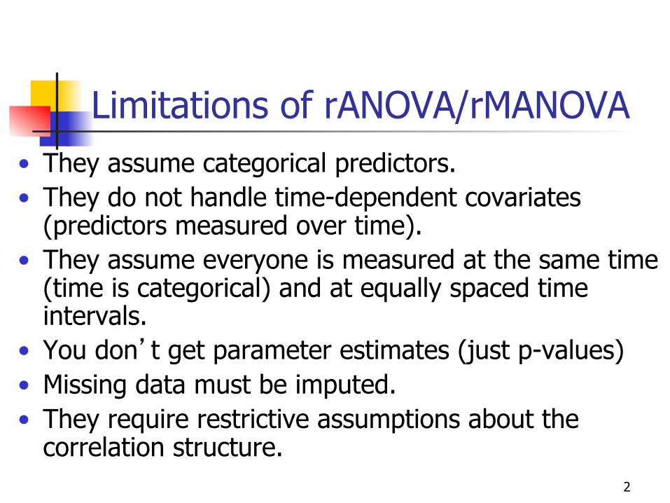
Limitations of rANOVA/rMANOVA • They assume categorical predictors. • They do not handle time-dependent covariates
(predictors measured over time). • They assume everyone is measured at the same time
(time is categorical) and at equally spaced time intervals.
• You don’t get parameter estimates (just p-values) • Missing data must be imputed. • They require restrictive assumptions about the
correlation structure.
3
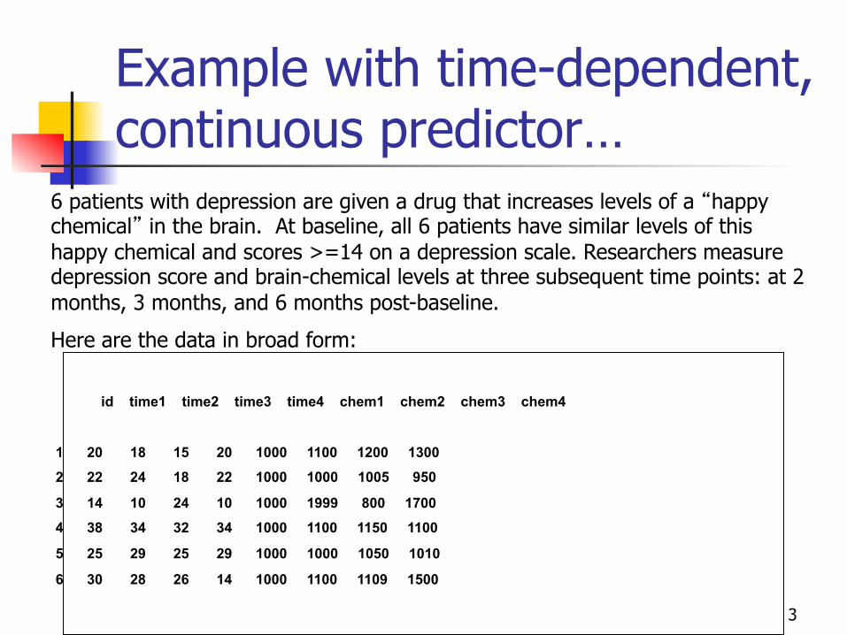
Example with time-dependent, continuous predictor…
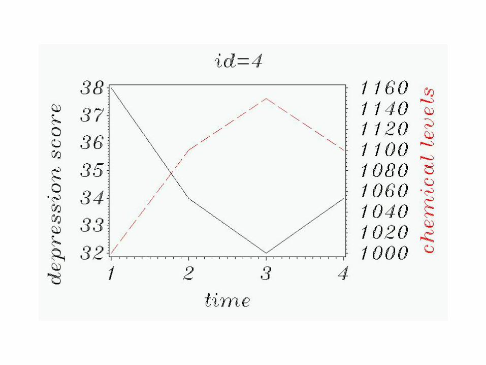
id time1 time2 time3 time4 chem1 chem2 chem3 chem4
1 20 18 15 20 1000 1100 1200 1300
2 22 24 18 22 1000 1000 1005 950
3 14 10 24 10 1000 1999 800 1700
4 38 34 32 34 1000 1100 1150 1100
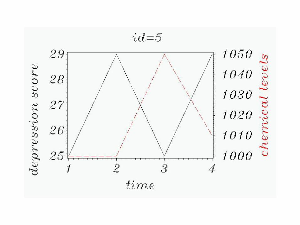
5 25 29 25 29 1000 1000 1050 1010
6 30 28 26 14 1000 1100 1109 1500
6 patients with depression are given a drug that increases levels of a “happy chemical” in the brain. At baseline, all 6 patients have similar levels of this happy chemical and scores >=14 on a depression scale. Researchers measure depression score and brain-chemical levels at three subsequent time points: at 2 months, 3 months, and 6 months post-baseline.
Here are the data in broad form:
4
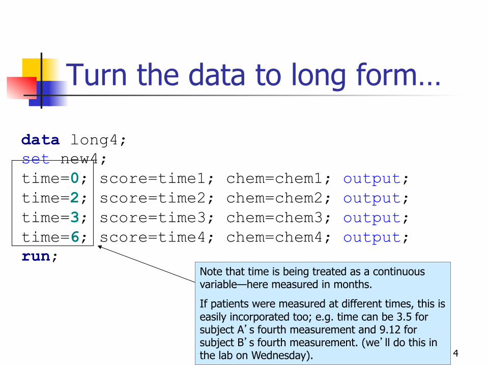
Turn the data to long form…
data long4; set new4; time=0; score=time1; chem=chem1; output; time=2; score=time2; chem=chem2; output; time=3; score=time3; chem=chem3; output; time=6; score=time4; chem=chem4; output; run;
Note that time is being treated as a continuous variable—here measured in months.
If patients were measured at different times, this is easily incorporated too; e.g. time can be 3.5 for subject A’s fourth measurement and 9.12 for subject B’s fourth measurement. (we’ll do this in the lab on Wednesday).
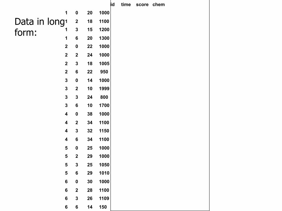
Data in long form:
id time score chem
1 0 20 1000
1 2 18 1100
1 3 15 1200
1 6 20 1300
2 0 22 1000
2 2 24 1000
2 3 18 1005
2 6 22 950
3 0 14 1000
3 2 10 1999
3 3 24 800
3 6 10 1700
4 0 38 1000
4 2 34 1100
4 3 32 1150
4 6 34 1100
5 0 25 1000
5 2 29 1000
5 3 25 1050
5 6 29 1010
6 0 30 1000
6 2 28 1100
6 3 26 1109
6 6 14 150
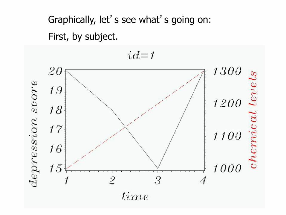
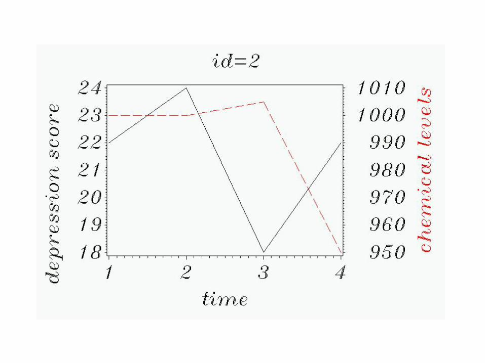
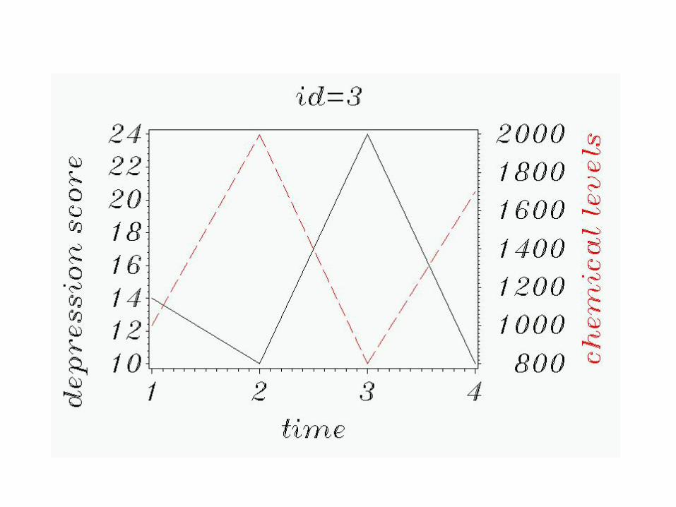
Graphically, let’s see what’s going on:
First, by subject.

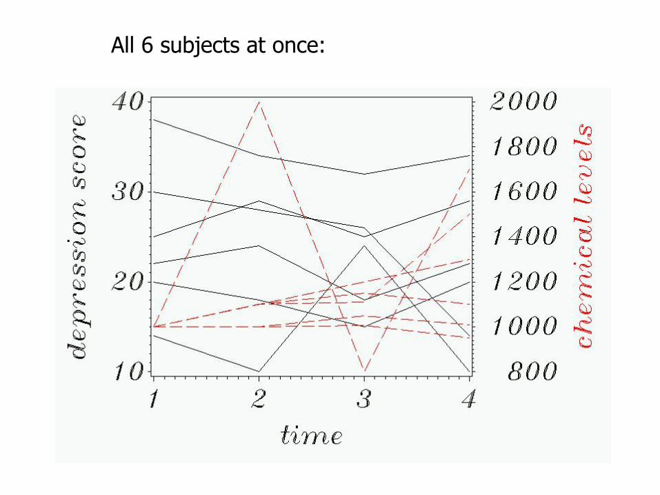
All 6 subjects at once:
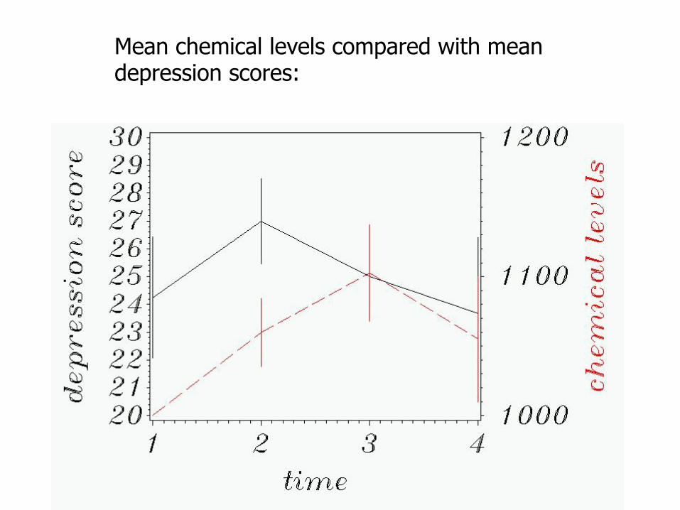
Mean chemical levels compared with mean depression scores:

14
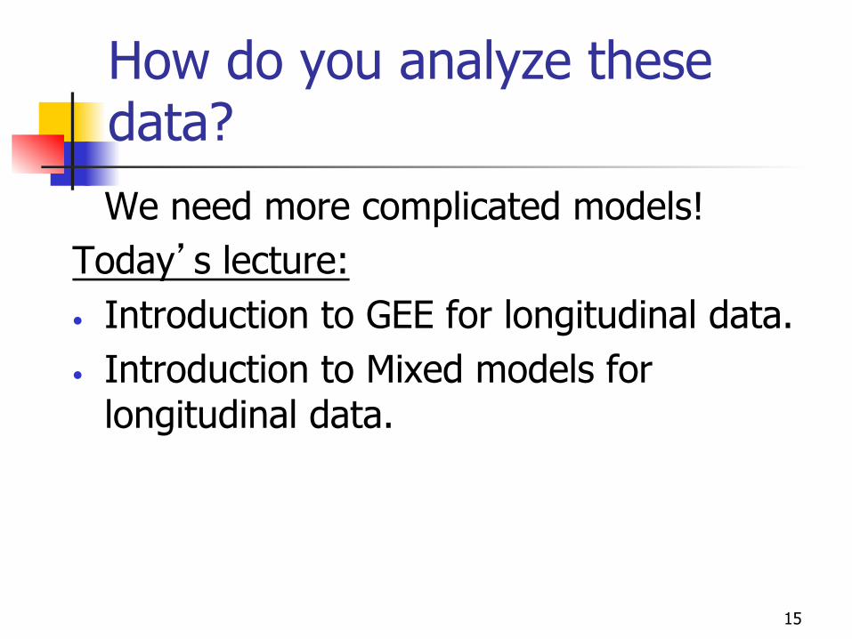
How do you analyze these data?
Using repeated-measures ANOVA? The only way to force a rANOVA here is… data forcedanova; set broad; avgchem=(chem1+chem2+chem3+chem4)/4; if avgchem<1100 then group="low"; if avgchem>1100 then group="high";
run; proc glm data=forcedanova; class group;
model time1-time4= group/ nouni; repeated time /summary;
run; quit;
Gives no significant results!
15
How do you analyze these data?
We need more complicated models! Today’s lecture: • Introduction to GEE for longitudinal data. • Introduction to Mixed models for
longitudinal data.

16
But first…naïve analysis… n The data in long form could be naively thrown into
an ordinary least squares (OLS) linear regression… n I.e., look for a linear correlation between chemical
levels and depression scores ignoring the correlation between subjects. (the cheating way to get 4-times as much data!)
n Can also look for a linear correlation between depression scores and time.
n In SAS:
proc reg data=long; model score=chem time; run;

17
Graphically… Naïve linear regression here looks for significant slopes (ignoring correlation between individuals):
N=24—as if we have 24 independent observations!
Y=42.44831-0.01685*chem Y= 24.90889 - 0.557778*time.

18
The model
The linear regression model:
iitimeichemi ErrortimechemY +++= )()(0 βββ
19
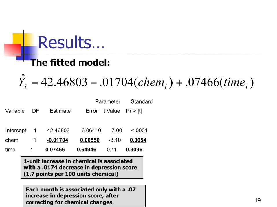
Results…
Parameter Standard
Variable DF Estimate Error t Value Pr > |t|
Intercept 1 42.46803 6.06410 7.00 <.0001
chem 1 -0.01704 0.00550 -3.10 0.0054
time 1 0.07466 0.64946 0.11 0.9096
1-unit increase in chemical is associated with a .0174 decrease in depression score (1.7 points per 100 units chemical)
Each month is associated only with a .07 increase in depression score, after correcting for chemical changes.
The fitted model:
)(07466.)(01704.46803.42ˆiii timechemY +−=
20
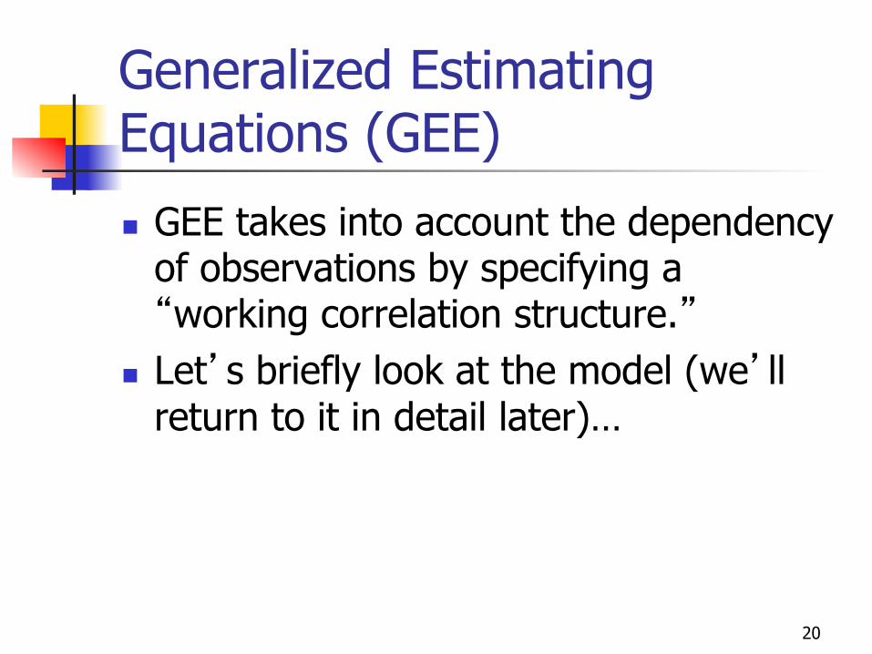
Generalized Estimating Equations (GEE)
n GEE takes into account the dependency of observations by specifying a “working correlation structure.”
n Let’s briefly look at the model (we’ll return to it in detail later)…
21
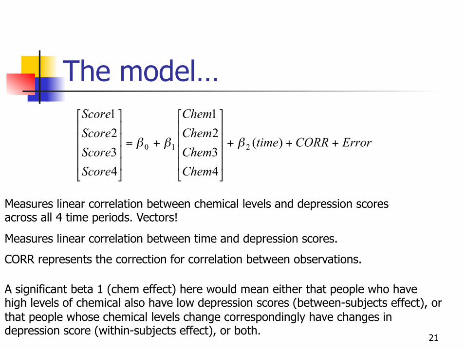
ErrorCORRtime
ChemChemChemChem
ScoreScoreScoreScore
+++
!!!!
"
#
$$$$
%
&
+=
!!!!
"
#
$$$$
%
&
)(
4321
4321
210 βββ
Measures linear correlation between chemical levels and depression scores across all 4 time periods. Vectors!
Measures linear correlation between time and depression scores.
CORR represents the correction for correlation between observations.
The model…
A significant beta 1 (chem effect) here would mean either that people who have high levels of chemical also have low depression scores (between-subjects effect), or that people whose chemical levels change correspondingly have changes in depression score (within-subjects effect), or both.

22
SAS code (long form of data!!)
proc genmod data=long4; class id; model score=chem time; repeated subject = id / type=exch corrw; run; quit;
Time is continuous (do not place on class statement)!
Here we are modeling as a linear relationship with score.
The type of correlation structure…
Generalized Linear models (using MLE)…
NOTE, for time-dependent predictors… --Interaction term with time (e.g. chem*time) is NOT necessary to get a within-subjects effect.
--Would only be included if you thought there was an acceleration or deceleration of the chem effect with time.
23
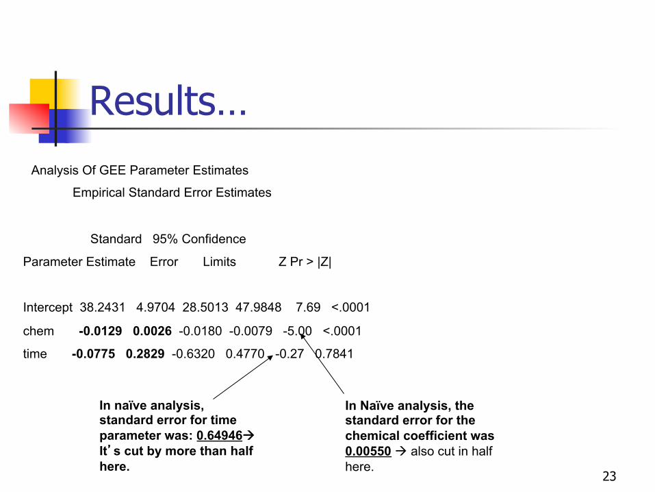
Results… Analysis Of GEE Parameter Estimates
Empirical Standard Error Estimates
Standard 95% Confidence
Parameter Estimate Error Limits Z Pr > |Z|
Intercept 38.2431 4.9704 28.5013 47.9848 7.69 <.0001
chem -0.0129 0.0026 -0.0180 -0.0079 -5.00 <.0001
time -0.0775 0.2829 -0.6320 0.4770 -0.27 0.7841
In naïve analysis, standard error for time parameter was: 0.64946 It’s cut by more than half here.
In Naïve analysis, the standard error for the chemical coefficient was 0.00550 à also cut in half here.
24
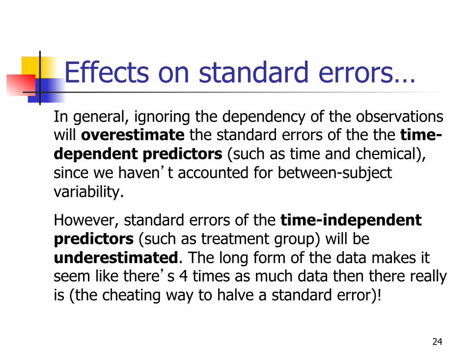
Effects on standard errors… In general, ignoring the dependency of the observations will overestimate the standard errors of the the time-dependent predictors (such as time and chemical), since we haven’t accounted for between-subject variability.
However, standard errors of the time-independent predictors (such as treatment group) will be underestimated. The long form of the data makes it seem like there’s 4 times as much data then there really is (the cheating way to halve a standard error)!
25
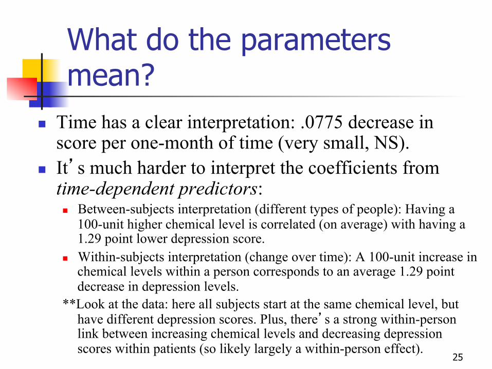
What do the parameters mean?
n Time has a clear interpretation: .0775 decrease in score per one-month of time (very small, NS).
n It’s much harder to interpret the coefficients from time-dependent predictors: n Between-subjects interpretation (different types of people): Having a
100-unit higher chemical level is correlated (on average) with having a 1.29 point lower depression score.
n Within-subjects interpretation (change over time): A 100-unit increase in chemical levels within a person corresponds to an average 1.29 point decrease in depression levels.
**Look at the data: here all subjects start at the same chemical level, but have different depression scores. Plus, there’s a strong within-person link between increasing chemical levels and decreasing depression scores within patients (so likely largely a within-person effect).
26
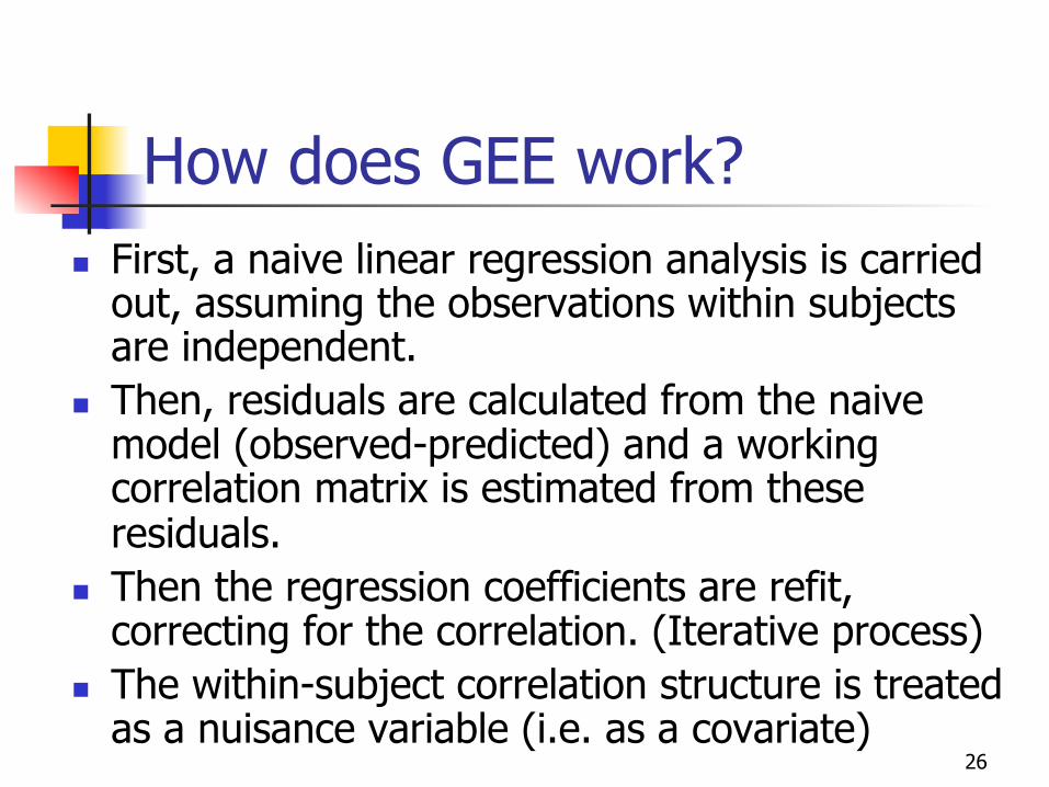
How does GEE work? n First, a naive linear regression analysis is carried
out, assuming the observations within subjects are independent.
n Then, residuals are calculated from the naive model (observed-predicted) and a working correlation matrix is estimated from these residuals.
n Then the regression coefficients are refit, correcting for the correlation. (Iterative process)
n The within-subject correlation structure is treated as a nuisance variable (i.e. as a covariate)
27
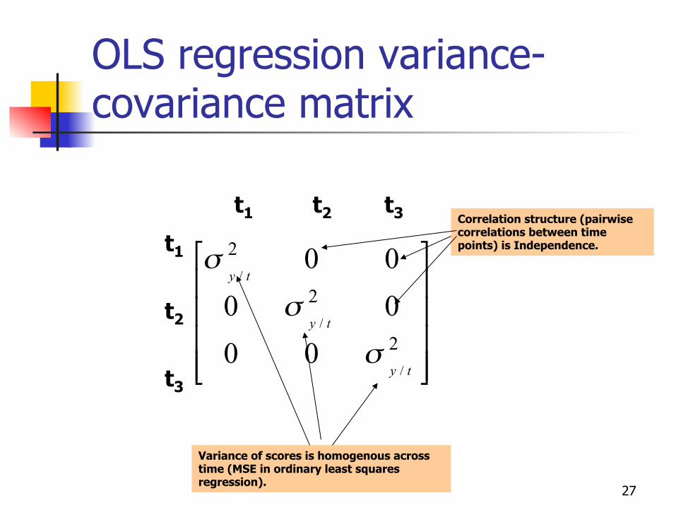
OLS regression variance-covariance matrix
!!!!
"
#
$$$$
%
&
2
2
2
/
/
/
000000
ty
ty
ty
σ
σ
σ
t1 t2 t3
t1
t2
t3
Variance of scores is homogenous across time (MSE in ordinary least squares regression).
Correlation structure (pairwise correlations between time points) is Independence.
28
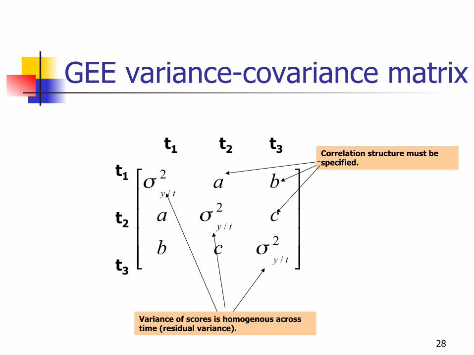
GEE variance-covariance matrix
!!!!
"
#
$$$$
%
&
2
2
2
/
/
/
ty
ty
ty
cbcaba
σ
σ
σ
t1 t2 t3
t1
t2
t3
Variance of scores is homogenous across time (residual variance).
Correlation structure must be specified.

29
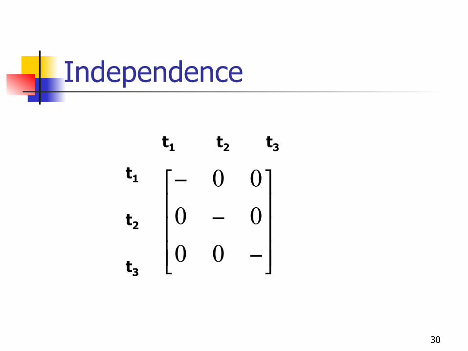
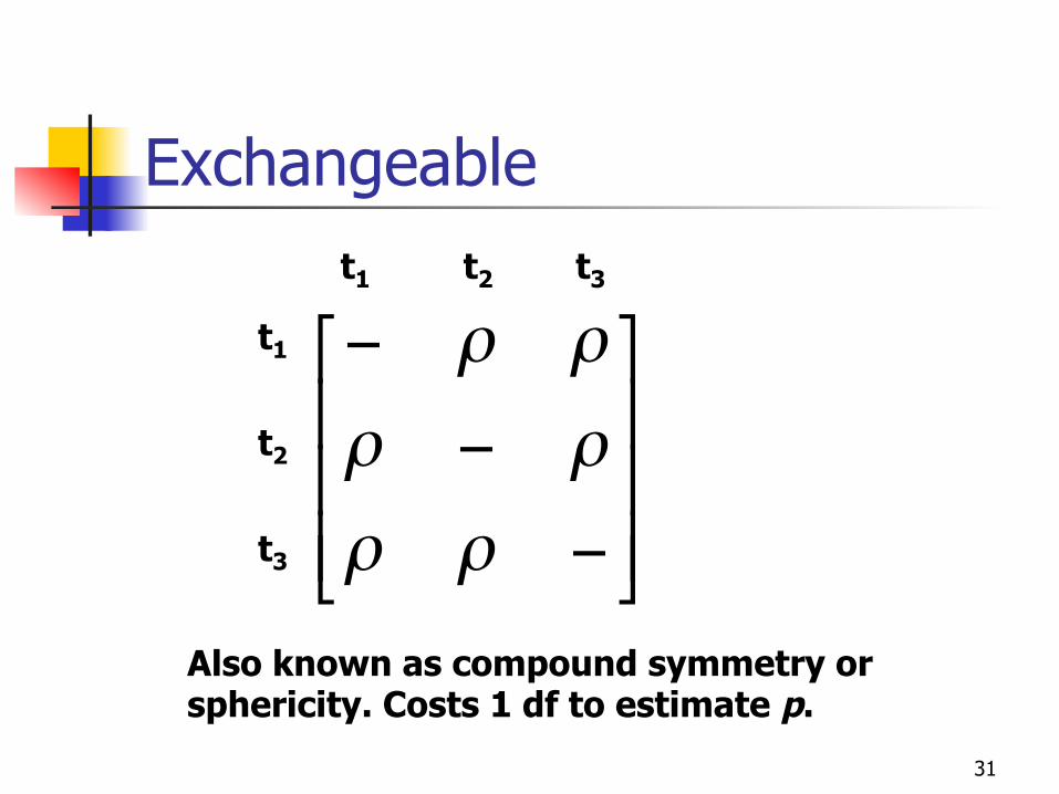
Choice of the correlation structure within GEE
In GEE, the correction for within subject correlations is carried out by assuming a priori a correlation structure for the repeated measurements (although GEE is fairly robust against a wrong choice of correlation matrix—particularly with large sample size) Choices:
• Independent (naïve analysis) • Exchangeable (compound symmetry, as in rANOVA) • Autoregressive • M-dependent • Unstructured (no specification, as in rMANOVA)
We are looking for the simplest structure (uses up the fewest degrees of freedom) that fits data well!
30
Independence
!!!
"
#
$$$
%
&
−
−
−
000000
t1 t2 t3
t1
t2
t3
31
Exchangeable
Also known as compound symmetry or sphericity. Costs 1 df to estimate p.
!!!
"
#
$$$
%
&
−
−
−
ρρ
ρρ
ρρ t1 t2 t3
t1
t2
t3
32
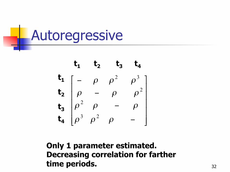
Autoregressive
!!!!!
"
#
$$$$$
%
&
−
−
−
−
23
2
2
32
ρρρ
ρρρ
ρρρ
ρρρ
t1 t2 t3 t4
t1 t2 t3 t4
Only 1 parameter estimated. Decreasing correlation for farther time periods.
33
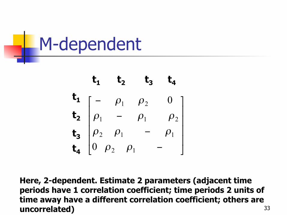
M-dependent
!!!!
"
#
$$$$
%
&
−
−
−
−
0
0
12
112
211
21
ρρ
ρρρ
ρρρ
ρρ
t1 t2 t3 t4
t1 t2 t3 t4
Here, 2-dependent. Estimate 2 parameters (adjacent time periods have 1 correlation coefficient; time periods 2 units of time away have a different correlation coefficient; others are uncorrelated)
34
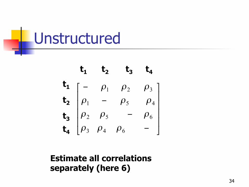
Unstructured
!!!!
"
#
$$$$
%
&
−
−
−
−
643
652
451
321
ρρρ
ρρρ
ρρρ
ρρρ
t1 t2 t3 t4
t1 t2 t3 t4
Estimate all correlations separately (here 6)
35
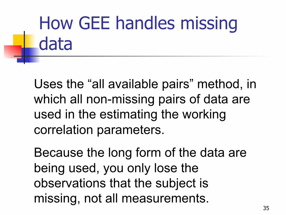
How GEE handles missing data
Uses the “all available pairs” method, in which all non-missing pairs of data are used in the estimating the working correlation parameters.
Because the long form of the data are being used, you only lose the observations that the subject is missing, not all measurements.
36
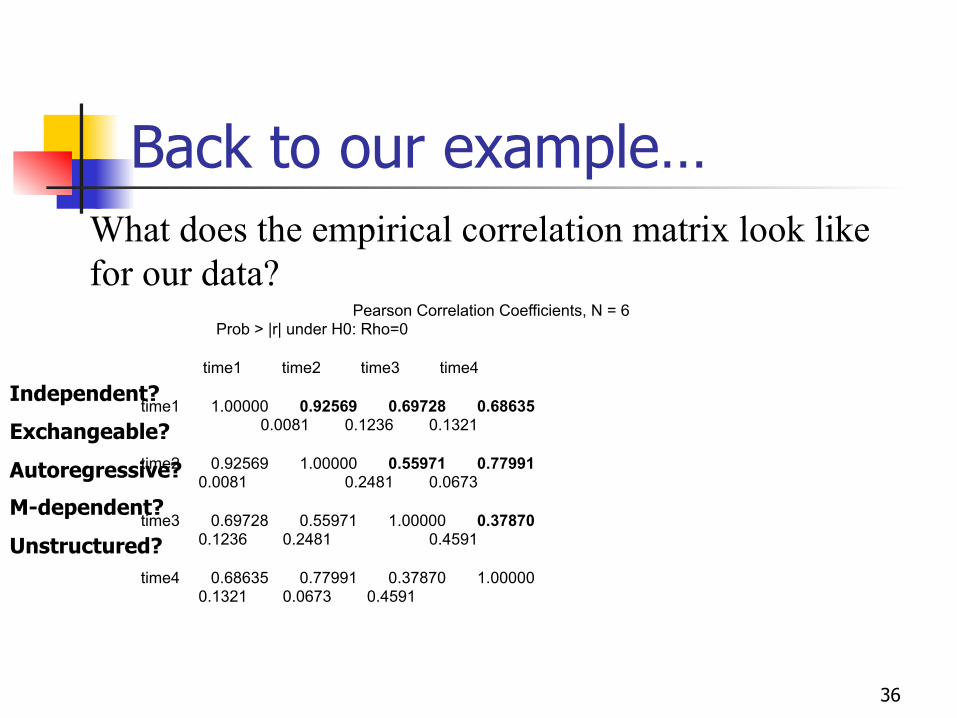
Back to our example… What does the empirical correlation matrix look like for our data?
Pearson Correlation Coefficients, N = 6 Prob > |r| under H0: Rho=0 time1 time2 time3 time4 time1 1.00000 0.92569 0.69728 0.68635 0.0081 0.1236 0.1321 time2 0.92569 1.00000 0.55971 0.77991 0.0081 0.2481 0.0673 time3 0.69728 0.55971 1.00000 0.37870 0.1236 0.2481 0.4591 time4 0.68635 0.77991 0.37870 1.00000 0.1321 0.0673 0.4591
Independent?
Exchangeable?
Autoregressive?
M-dependent?
Unstructured?
37
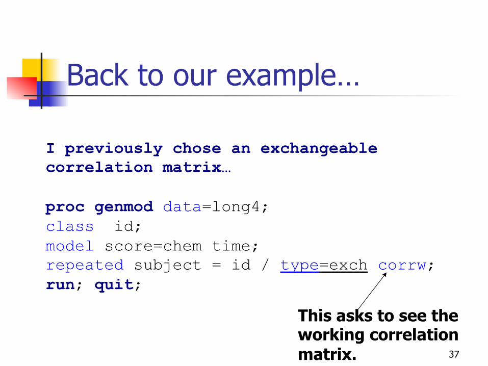
Back to our example…
I previously chose an exchangeable correlation matrix… proc genmod data=long4; class id; model score=chem time; repeated subject = id / type=exch corrw; run; quit;
This asks to see the working correlation matrix.

38
Working Correlation Matrix Working Correlation Matrix Col1 Col2 Col3 Col4 Row1 1.0000 0.7276 0.7276 0.7276 Row2 0.7276 1.0000 0.7276 0.7276 Row3 0.7276 0.7276 1.0000 0.7276 Row4 0.7276 0.7276 0.7276 1.0000
Standard 95% Confidence
Parameter Estimate Error Limits Z Pr > |Z|
Intercept 38.2431 4.9704 28.5013 47.9848 7.69 <.0001
chem -0.0129 0.0026 -0.0180 -0.0079 -5.00 <.0001
time -0.0775 0.2829 -0.6320 0.4770 -0.27 0.7841

39
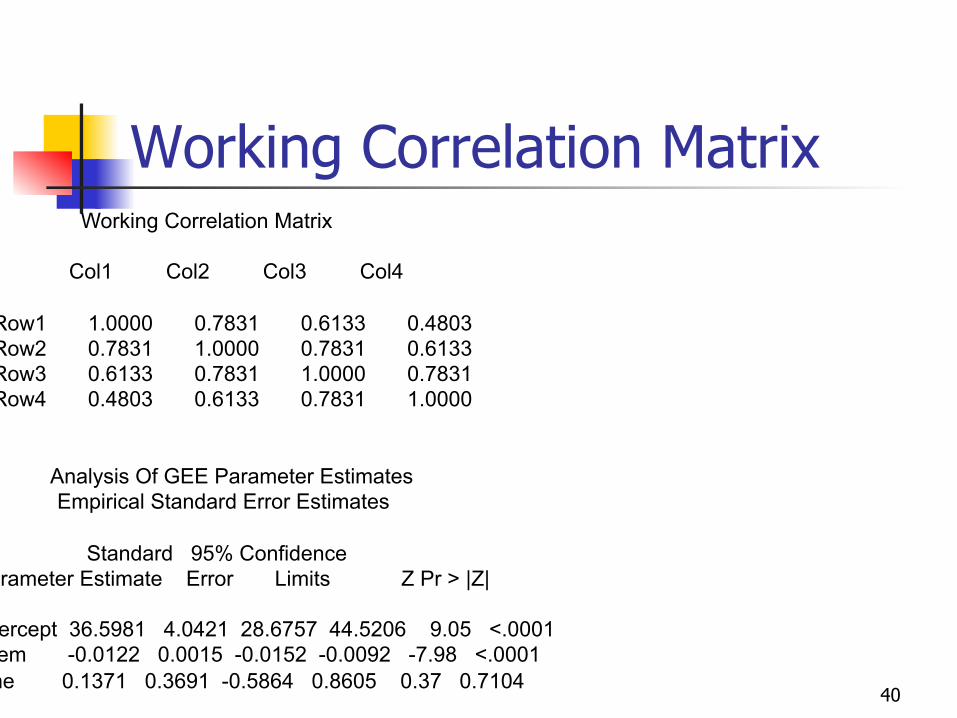
Compare to autoregressive…
proc genmod data=long4;
class id;
model score=chem time;
repeated subject = id / type=ar corrw;
run; quit;
40
Working Correlation Matrix Working Correlation Matrix Col1 Col2 Col3 Col4 Row1 1.0000 0.7831 0.6133 0.4803 Row2 0.7831 1.0000 0.7831 0.6133 Row3 0.6133 0.7831 1.0000 0.7831 Row4 0.4803 0.6133 0.7831 1.0000 Analysis Of GEE Parameter Estimates Empirical Standard Error Estimates Standard 95% Confidence Parameter Estimate Error Limits Z Pr > |Z| Intercept 36.5981 4.0421 28.6757 44.5206 9.05 <.0001 chem -0.0122 0.0015 -0.0152 -0.0092 -7.98 <.0001 time 0.1371 0.3691 -0.5864 0.8605 0.37 0.7104
41
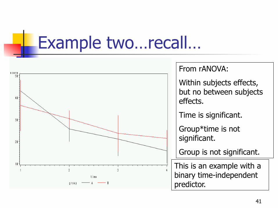
Example two…recall… From rANOVA:
Within subjects effects, but no between subjects effects.
Time is significant.
Group*time is not significant.
Group is not significant.
This is an example with a binary time-independent predictor.
42
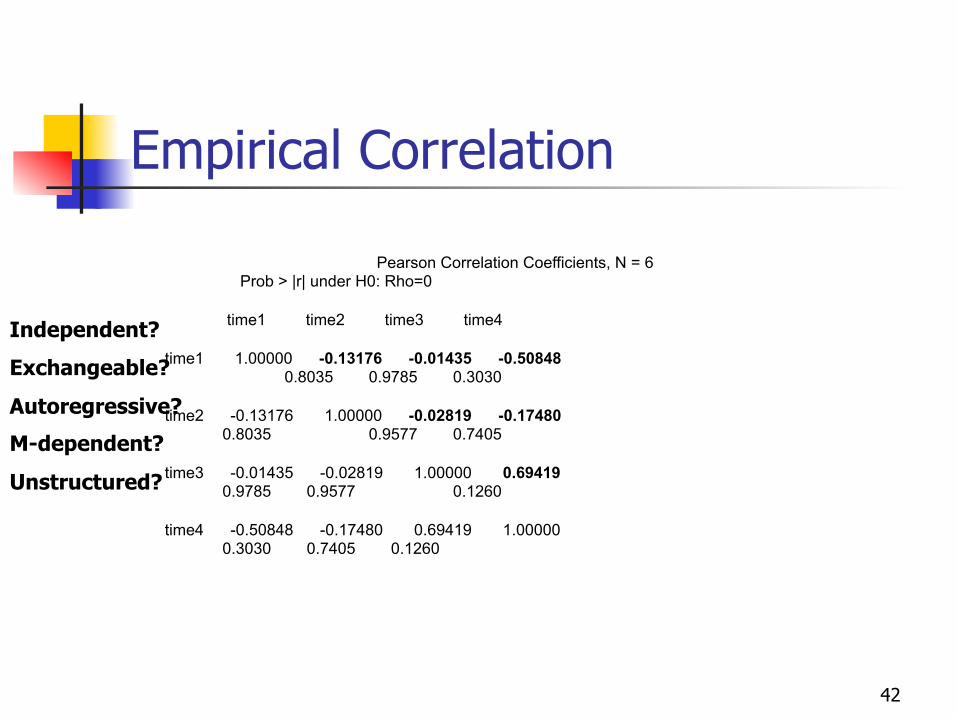
Empirical Correlation
Pearson Correlation Coefficients, N = 6 Prob > |r| under H0: Rho=0 time1 time2 time3 time4 time1 1.00000 -0.13176 -0.01435 -0.50848 0.8035 0.9785 0.3030 time2 -0.13176 1.00000 -0.02819 -0.17480 0.8035 0.9577 0.7405 time3 -0.01435 -0.02819 1.00000 0.69419 0.9785 0.9577 0.1260 time4 -0.50848 -0.17480 0.69419 1.00000 0.3030 0.7405 0.1260
Independent?
Exchangeable?
Autoregressive?
M-dependent?
Unstructured?
43
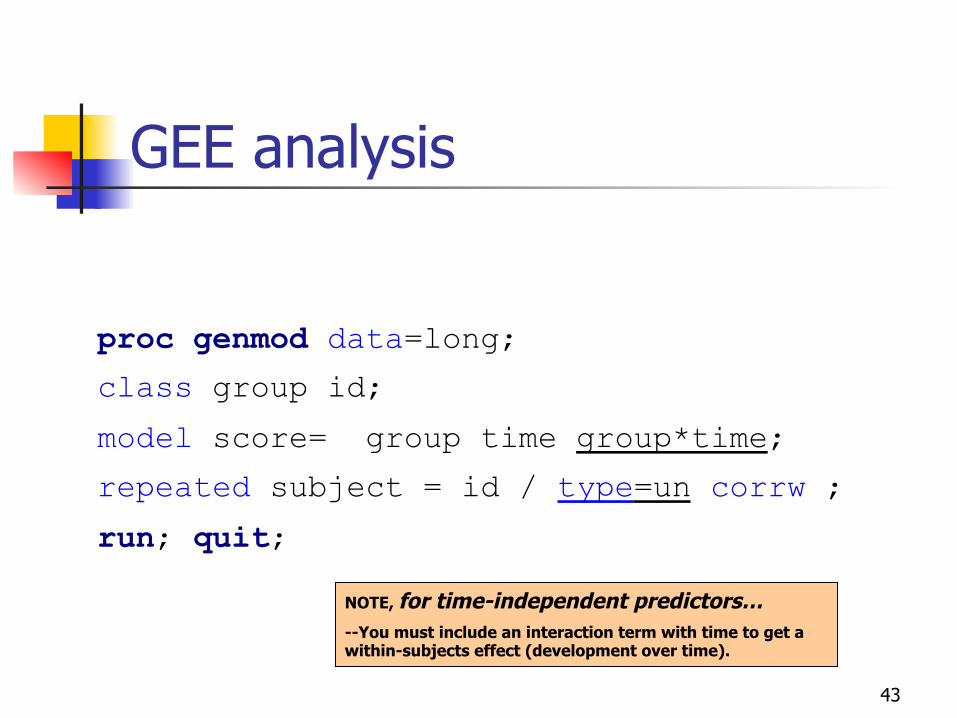
GEE analysis
proc genmod data=long;
class group id;
model score= group time group*time;
repeated subject = id / type=un corrw ;
run; quit;
NOTE, for time-independent predictors… --You must include an interaction term with time to get a within-subjects effect (development over time).
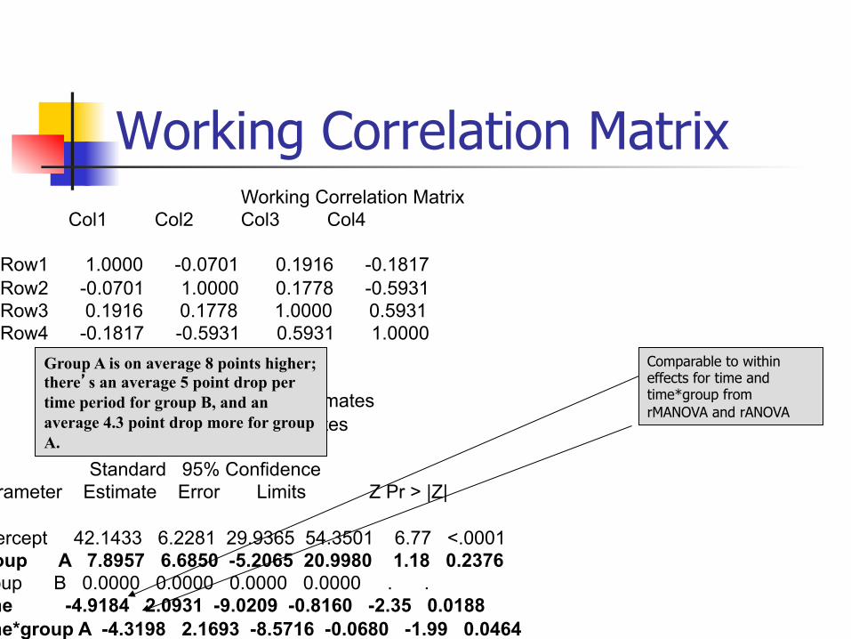
Working Correlation Matrix Working Correlation Matrix Col1 Col2 Col3 Col4 Row1 1.0000 -0.0701 0.1916 -0.1817 Row2 -0.0701 1.0000 0.1778 -0.5931 Row3 0.1916 0.1778 1.0000 0.5931 Row4 -0.1817 -0.5931 0.5931 1.0000 Analysis Of GEE Parameter Estimates Empirical Standard Error Estimates Standard 95% Confidence Parameter Estimate Error Limits Z Pr > |Z| Intercept 42.1433 6.2281 29.9365 54.3501 6.77 <.0001 group A 7.8957 6.6850 -5.2065 20.9980 1.18 0.2376 group B 0.0000 0.0000 0.0000 0.0000 . . time -4.9184 2.0931 -9.0209 -0.8160 -2.35 0.0188 time*group A -4.3198 2.1693 -8.5716 -0.0680 -1.99 0.0464
Group A is on average 8 points higher; there’s an average 5 point drop per time period for group B, and an average 4.3 point drop more for group A.
Comparable to within effects for time and time*group from rMANOVA and rANOVA
45
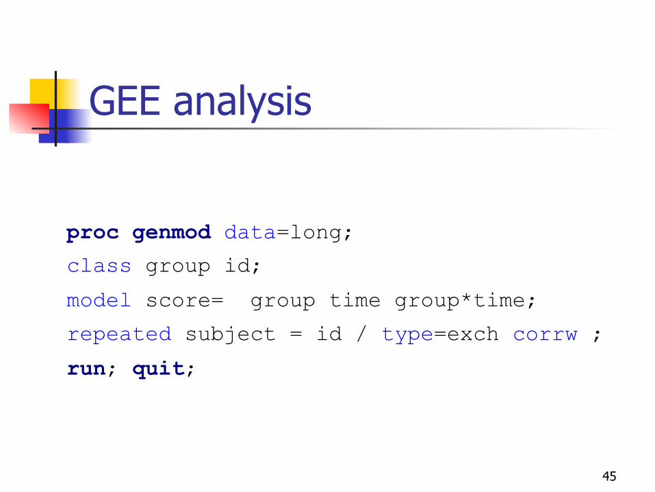
GEE analysis
proc genmod data=long;
class group id;
model score= group time group*time;
repeated subject = id / type=exch corrw ;
run; quit;

Working Correlation Matrix Working Correlation Matrix Col1 Col2 Col3 Col4 Row1 1.0000 -0.0529 -0.0529 -0.0529 Row2 -0.0529 1.0000 -0.0529 -0.0529 Row3 -0.0529 -0.0529 1.0000 -0.0529 Row4 -0.0529 -0.0529 -0.0529 1.0000 Analysis Of GEE Parameter Estimates Empirical Standard Error Estimates Standard 95% Confidence Parameter Estimate Error Limits Z Pr > |Z| Intercept 40.8333 5.8516 29.3645 52.3022 6.98 <.0001 group A 7.1667 6.1974 -4.9800 19.3133 1.16 0.2475 group B 0.0000 0.0000 0.0000 0.0000 . . time -5.1667 1.9461 -8.9810 -1.3523 -2.65 0.0079 time*group A -3.5000 2.2885 -7.9853 0.9853 -1.53 0.1262
P-values are similar to rANOVA (which of course assumed exchangeable, or compound symmetry, for the correlation structure!)
47
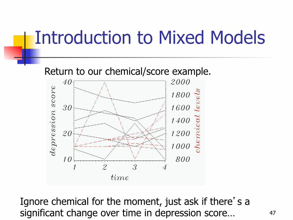
Introduction to Mixed Models
Return to our chemical/score example.
Ignore chemical for the moment, just ask if there’s a significant change over time in depression score…
48
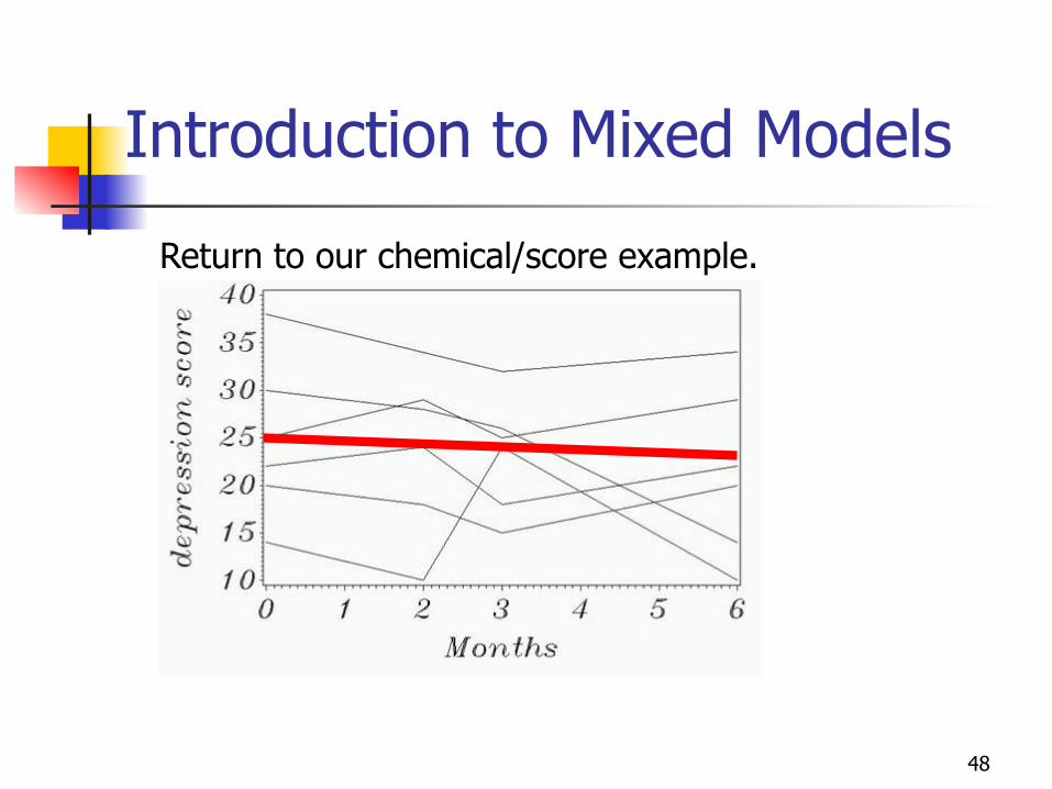
Introduction to Mixed Models
Return to our chemical/score example.
49
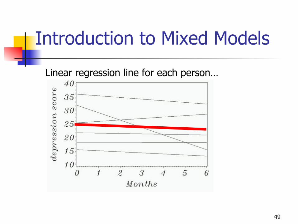
Introduction to Mixed Models
Linear regression line for each person…

50
Introduction to Mixed Models
Mixed models = fixed and random effects. For example,
itfixedtimerandomiitY εββ ++= )()(0
),(~ 200 0β
σββ populationi N
constant=timeβ
Treated as a random variable with a probability distribution.
This variance is comparable to the between-subjects variance from rANOVA.
),0(~ 2/ ty
N σResidual variance:
Two parameters to estimate instead of 1
51
Introduction to Mixed Models
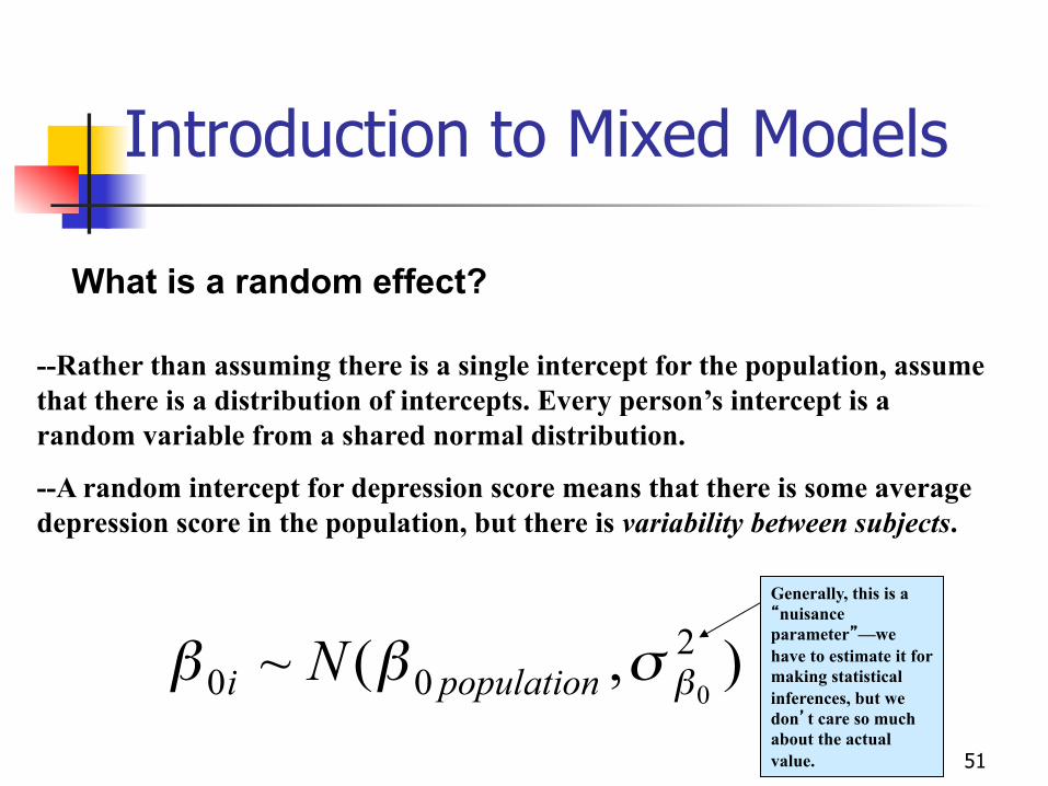
What is a random effect?
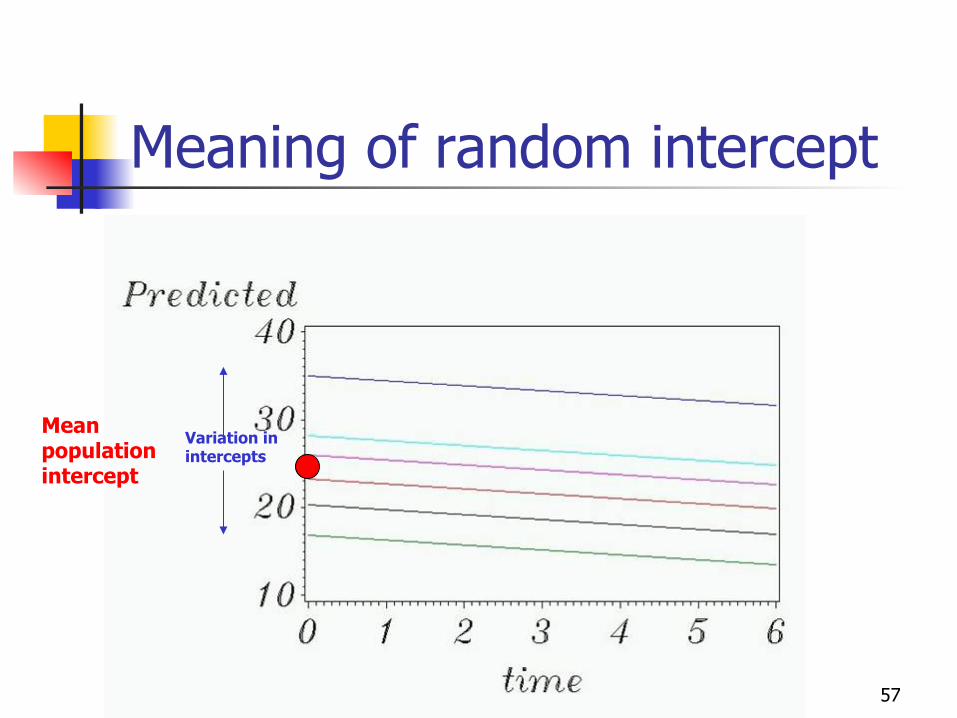
--Rather than assuming there is a single intercept for the population, assume that there is a distribution of intercepts. Every person’s intercept is a random variable from a shared normal distribution.
--A random intercept for depression score means that there is some average depression score in the population, but there is variability between subjects.
),(~ 200 0β
σββ populationi NGenerally, this is a “nuisance parameter”—we have to estimate it for making statistical inferences, but we don’t care so much about the actual value.
52
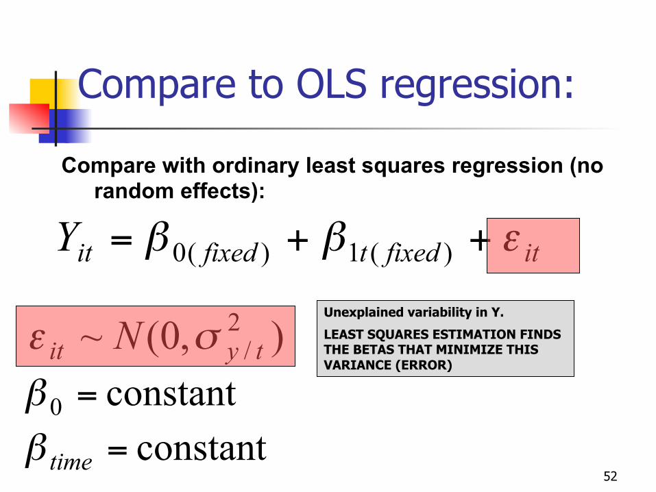
Compare to OLS regression:
Compare with ordinary least squares regression (no random effects):
itfixedtfixeditY εββ ++= )(1)(0
constant0 =β
Unexplained variability in Y.
LEAST SQUARES ESTIMATION FINDS THE BETAS THAT MINIMIZE THIS VARIANCE (ERROR)
constant=timeβ
),0(~ 2/ tyit N σε
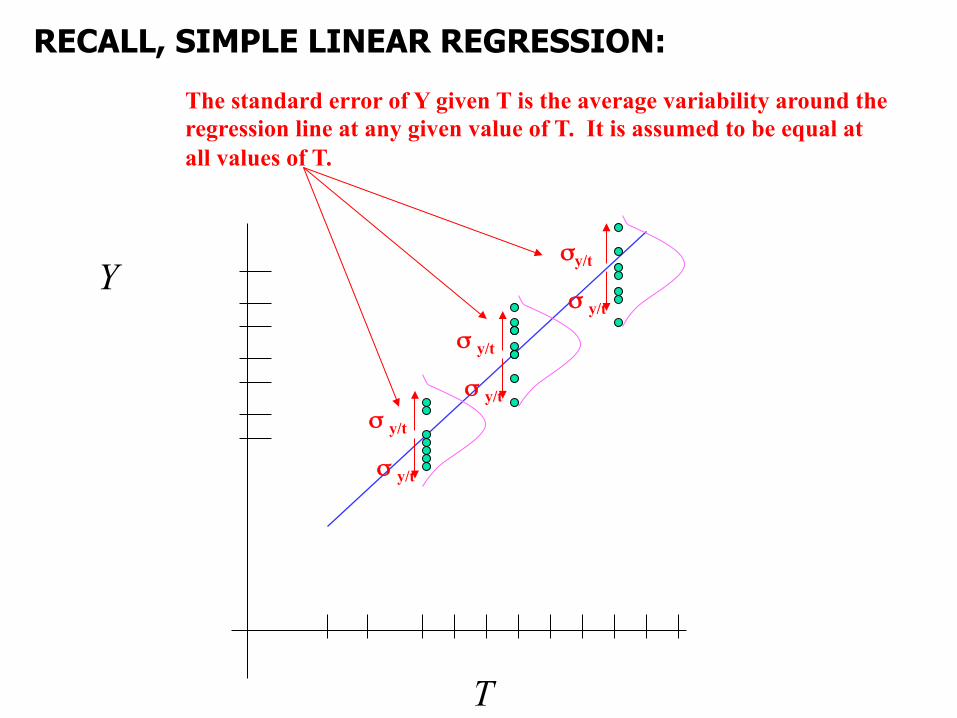
Y
T
The standard error of Y given T is the average variability around the regression line at any given value of T. It is assumed to be equal at all values of T.
σy/t
σ y/t
σ y/t
σ y/t
σ y/t
σ y/t
RECALL, SIMPLE LINEAR REGRESSION:
54
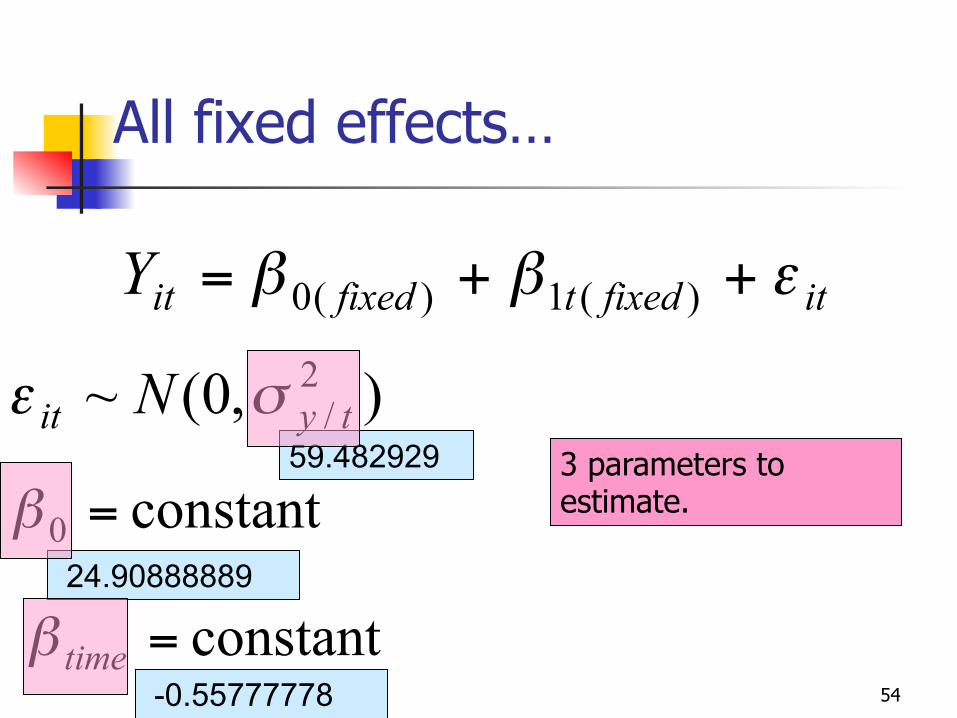
All fixed effects…
itfixedtfixeditY εββ ++= )(1)(0
constant0 =β59.482929
24.90888889
-0.55777778 constant=timeβ
),0(~ 2/ tyit N σε
3 parameters to estimate.
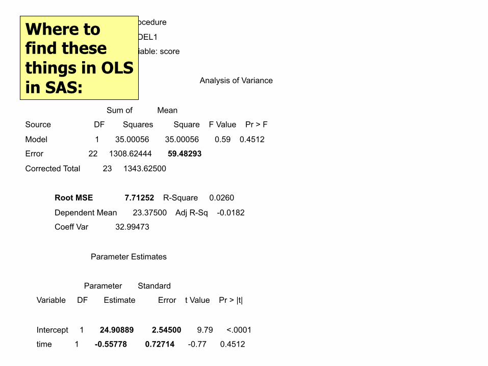
The REG Procedure
Model: MODEL1
Dependent Variable: score
Analysis of Variance
Sum of Mean
Source DF Squares Square F Value Pr > F
Model 1 35.00056 35.00056 0.59 0.4512
Error 22 1308.62444 59.48293
Corrected Total 23 1343.62500
Root MSE 7.71252 R-Square 0.0260
Dependent Mean 23.37500 Adj R-Sq -0.0182
Coeff Var 32.99473
Parameter Estimates
Parameter Standard
Variable DF Estimate Error t Value Pr > |t|
Intercept 1 24.90889 2.54500 9.79 <.0001
time 1 -0.55778 0.72714 -0.77 0.4512
Where to find these things in OLS in SAS:
56
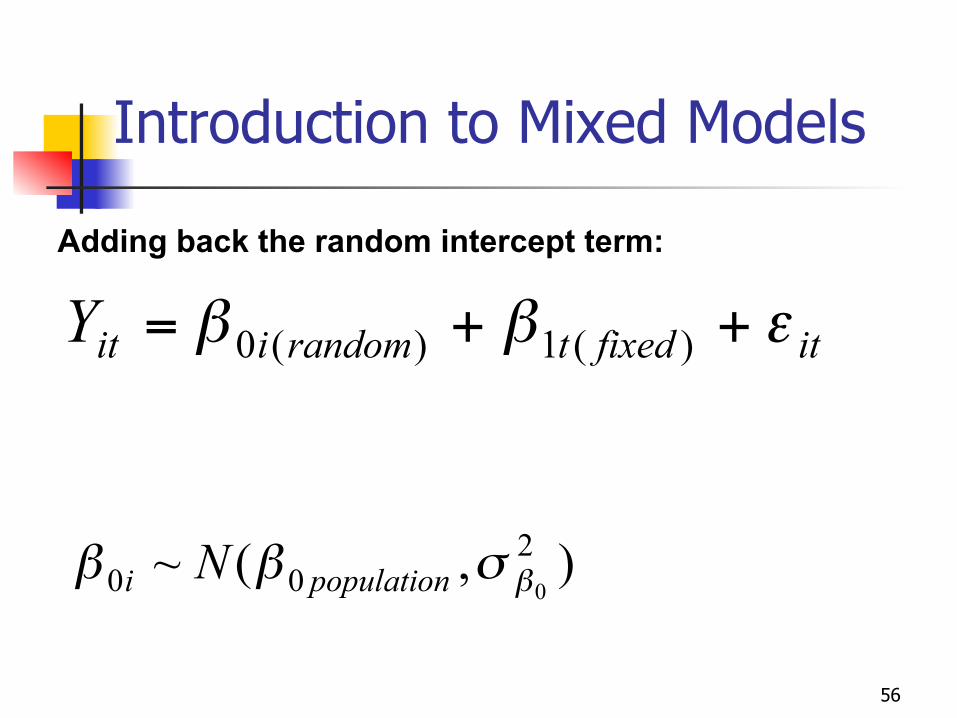
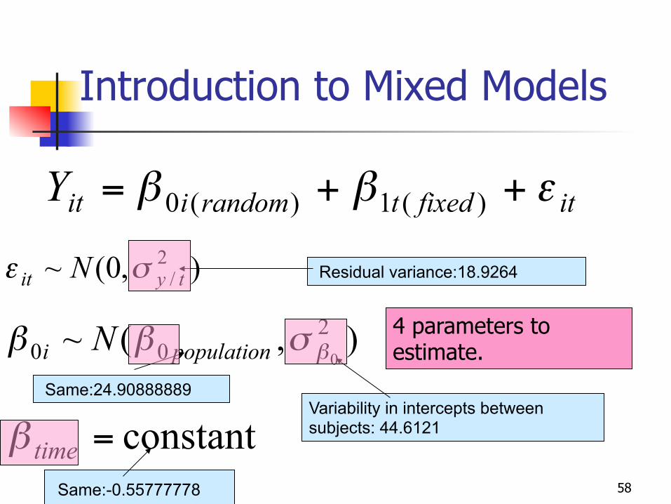
Introduction to Mixed Models
Adding back the random intercept term:
itfixedtrandomiitY εββ ++= )(1)(0
),(~ 200 0β
σββ populationi N
57
Meaning of random intercept
Mean population intercept
Variation in intercepts
58
Introduction to Mixed Models
itfixedtrandomiitY εββ ++= )(1)(0
),(~ 200 0β
σββ populationi N
Residual variance:18.9264
Variability in intercepts between subjects: 44.6121
Same:24.90888889
Same:-0.55777778
constant=timeβ
),0(~ 2/ tyit N σε
4 parameters to estimate.

Covariance Parameter Estimates
Cov Parm Subject Estimate
Variance id 44.6121
Residual 18.9264
Fit Statistics
-2 Res Log Likelihood 146.7
AIC (smaller is better) 152.7
AICC (smaller is better) 154.1
BIC (smaller is better) 152.1
Solution for Fixed Effects
Standard
Effect Estimate Error DF t Value Pr > |t|
Intercept 24.9089 3.0816 5 8.08 0.0005
time -0.5578 0.4102 17 -1.36 0.1916
Where to find these things in from MIXED in SAS:
Time coefficient is the same but standard error is nearly halved (from 0.72714)..
%696121.449264.18
6121.44=
+69% of variability in depression scores is explained by the differences between subjects
Interpretation is the same as with GEE: -.5578 decrease in score per month time.

60
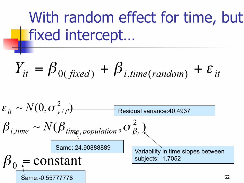
With random effect for time, but fixed intercept…
Allowing time-slopes to be random:
itrandomtimeifixeditY εββ ++= )(,)(0
),(~ 2,, tpopulationtimetimei N βσββ
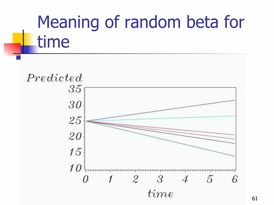
61
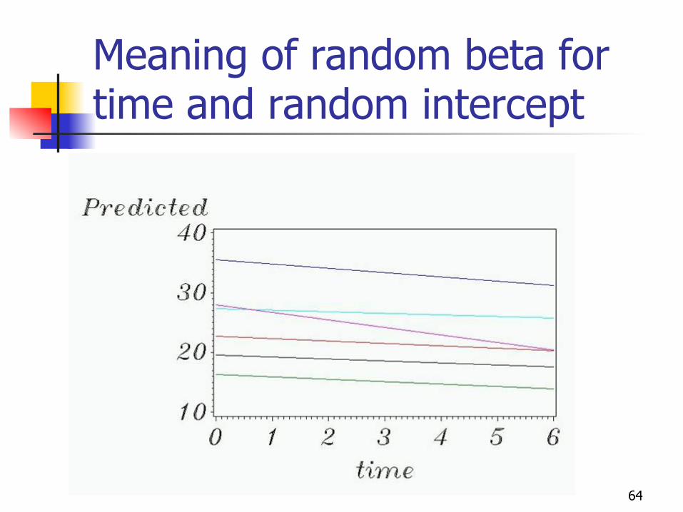
Meaning of random beta for time
62
With random effect for time, but fixed intercept…
itrandomtimeifixeditY εββ ++= )(,)(0
Variability in time slopes between subjects: 1.7052
Same: 24.90888889
Same:-0.55777778
constant0 =β
),(~ 2,, tpopulationtimetimei N βσββ
Residual variance:40.4937 ),0(~ 2/ tyit N σε
63
With both random…
With a random intercept and random time-slope:
itrandomtimeirandomiitY εββ ++= )(,)(0
),(~ 2,, tpopulationtimetimei N βσββ
),(~ 200 0β
σββ populationi N
64
Meaning of random beta for time and random intercept

65
With both random…
With a random intercept and random time-slope:
itrandomtimeirandomiitY εββ ++= )(,)(0
),(~ 2,, tpopulationtimetimei N βσββ
),(~ 200 0β
σββ populationi N 16.6311
53.0068
0.4162
24.90888889
0.55777778
Additionally, we have to estimate the covariance of the random intercept and random slope:
here -1.9943
(adding random time therefore cost us 2 degrees of freedom)
66
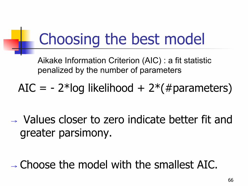
Choosing the best model
AIC = - 2*log likelihood + 2*(#parameters) → Values closer to zero indicate better fit and
greater parsimony.
→ Choose the model with the smallest AIC.
Aikake Information Criterion (AIC) : a fit statistic penalized by the number of parameters
67
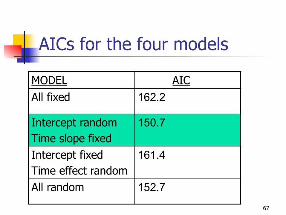
AICs for the four models
MODEL AIC All fixed 162.2
Intercept random Time slope fixed
150.7
Intercept fixed Time effect random
161.4
All random 152.7
68
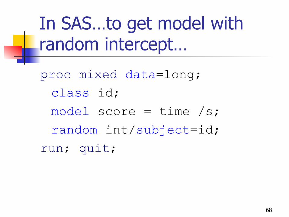
In SAS…to get model with random intercept…
proc mixed data=long; class id;
model score = time /s;
random int/subject=id;
run; quit;
69
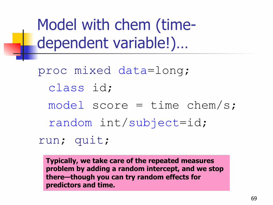
Model with chem (time-dependent variable!)…
proc mixed data=long; class id;
model score = time chem/s;
random int/subject=id;
run; quit;
Typically, we take care of the repeated measures problem by adding a random intercept, and we stop there—though you can try random effects for predictors and time.
Cov Parm Subject Estimate
Intercept id 35.5720
Residual 10.2504
Fit Statistics
-2 Res Log Likelihood 143.7
AIC (smaller is better) 147.7
AICC (smaller is better) 148.4
BIC (smaller is better) 147.3
Solution for Fixed Effects
Standard
Effect Estimate Error DF t Value Pr > |t|
Intercept 38.1287 4.1727 5 9.14 0.0003
time -0.08163 0.3234 16 -0.25 0.8039
chem -0.01283 0.003125 16 -4.11 0.0008
Residual and AIC are reduced even further due to strong explanatory power of chemical.
Interpretation is the same as with GEE: we cannot separate between-subjects and within-subjects effects of chemical.

71
New Example: time-independent binary predictor
From GEE:
Strong effect of time.
No group difference
Non-significant group*time trend.

72
SAS code…
proc mixed data=long ; class id group;
model score = time group time*group/s corrb;
random int /subject=id ;
run; quit;
73
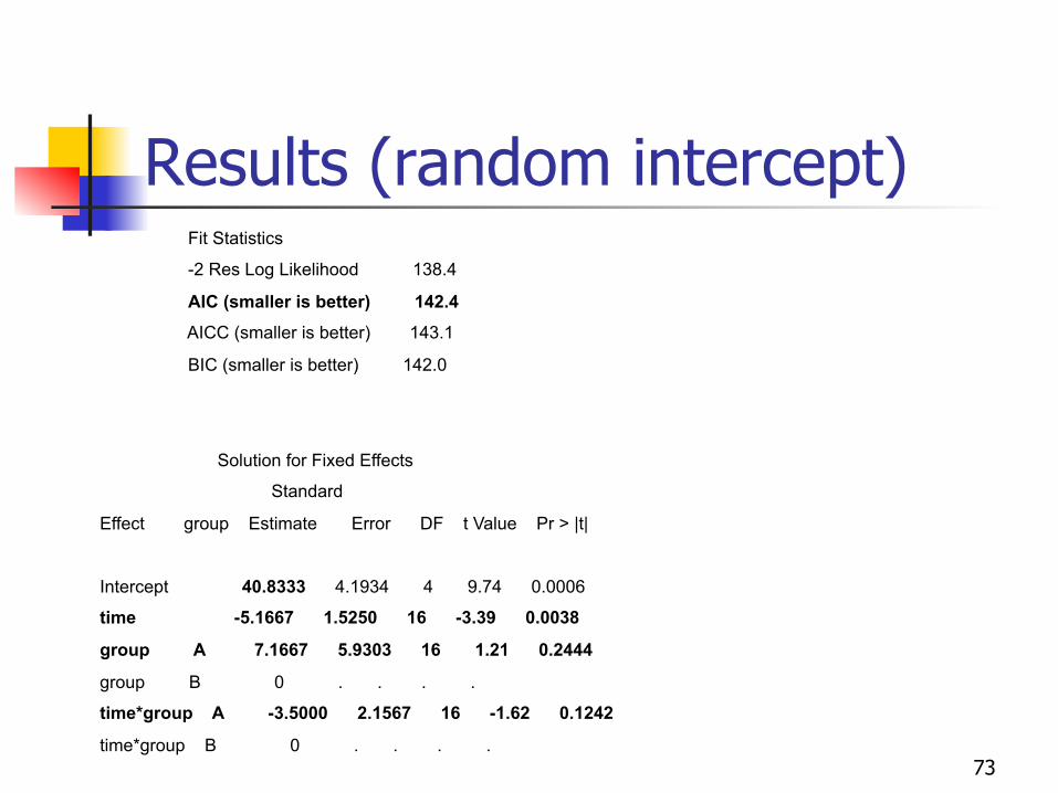
Results (random intercept) Fit Statistics
-2 Res Log Likelihood 138.4
AIC (smaller is better) 142.4
AICC (smaller is better) 143.1
BIC (smaller is better) 142.0
Solution for Fixed Effects
Standard
Effect group Estimate Error DF t Value Pr > |t|
Intercept 40.8333 4.1934 4 9.74 0.0006
time -5.1667 1.5250 16 -3.39 0.0038
group A 7.1667 5.9303 16 1.21 0.2444
group B 0 . . . .
time*group A -3.5000 2.1567 16 -1.62 0.1242
time*group B 0 . . . .
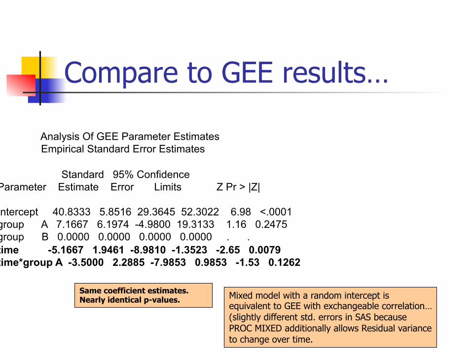
Compare to GEE results…
Same coefficient estimates. Nearly identical p-values.
Analysis Of GEE Parameter Estimates Empirical Standard Error Estimates Standard 95% Confidence Parameter Estimate Error Limits Z Pr > |Z| Intercept 40.8333 5.8516 29.3645 52.3022 6.98 <.0001 group A 7.1667 6.1974 -4.9800 19.3133 1.16 0.2475 group B 0.0000 0.0000 0.0000 0.0000 . . time -5.1667 1.9461 -8.9810 -1.3523 -2.65 0.0079 time*group A -3.5000 2.2885 -7.9853 0.9853 -1.53 0.1262
Mixed model with a random intercept is equivalent to GEE with exchangeable correlation…(slightly different std. errors in SAS because PROC MIXED additionally allows Residual variance to change over time.
75
Power of these models…
• Since these methods are based on generalized linear models, these methods can easily be extended to repeated measures with a dependent variable that is binary, categorical, or counts…
• These methods are not just for repeated measures. They are appropriate for any situation where dependencies arise in the data. For example,
• Studies across families (dependency within families) • Prevention trials where randomization is by school, practice, clinic, geographical area, etc. (dependency within unit of randomization) • Matched case-control studies (dependency within matched pair) • In general, anywhere you have “clusters” of observations (statisticians say that observations are “nested” within these clusters.) • For repeated measures, our “cluster” was the subject. • In the long form of the data, you have a variable that identifies which cluster the observation belongs too (for us, this was the variable “id”)
76
References n Jos W. R. Twisk. Applied Longitudinal Data Analysis for Epidemiology: A Practical
Guide. Cambridge University Press, 2003.