gd calc demo

1

Grating Diffraction Calculator (GD-Calc®) –

Demo and Tutorial Guide

Overview..................................................................................................................... 2 Demo 1a: Uniperiodic, sinusoidal grating .................................................................. 4 Demo 1b, 1c: Uniperiodic, sinusoidal grating (deep profile, metallic) ...................... 7 Demo 2: Biperiodic grating comprising rectangular pyramids................................... 9 Demo 3 and demo 4: Biperiodic checkerboard grating .............................................. 9 Demo 5: Biperiodic grating comprising circular pillars ........................................... 17 Demo 6 and 7: Biperiodic grating comprising a skewed metal grid........................ 21 Demo 8: Biperiodic grating comprising a square metal grid................................... 26 Demo 9: Alignment sensor ...................................................................................... 27 Demo10: Slanted lamellar grating ........................................................................... 30 Demo 11: Crossed-line grating ................................................................................ 32 Appendix A: Interface for gdc_demo_engine.p....................................................... 34 Appendix B. Algorithm notes for circle_partition.m............................................... 37

GD-Calc_Demo.pdf, version 09/22/2006 Copyright 2005-2006, Kenneth C. Johnson

software.kjinnovation.com

2

Overview GD-Calc is implemented in MATLAB® 1 and comprises the following files: Documentation:

- GD-Calc.pdf: Part 1 of GD-Calc.pdf explains the technical concepts, definitions and conventions upon which the software user interface is based. (You can defer reading this until after you’ve tried some of the demo scripts.) Part 2 details the theory and methods underlying the computation algorithm. (This part need not be read or understood to effectively use the software.)

- GD-Calc_Demo.pdf: To get started, skim through this document and try out some of the demo scripts. Refer to GD-Calc.pdf, Part 1, as needed, for clarification of the technical concepts.

Core functionality: - gdc.m: This is the entry point to the diffraction calculation engine. gdc.m

performs data validation and calls gdc_engine to run the actual calculations. (You can call gdc.m with no output arguments to just check data validity.)

- gdc_engine.p: the calculation engine. (Do not call gdc_engine directly – it is only intended to be called by gdc.)

Basic utilities (These may be revised and extended to better suit users’ needs.): - gdc_plot.m: for plotting grating structures. (gdc_plot.m calls gdc.m to check

data validity.) - gdc_eff.m: This function converts the output of gdc.m into diffraction

efficiency data. Demo programs (Users are encouraged to modify and generalize the demo scripts.):

- gdc_demo*.m: These demo scripts provide a tutorial introduction to GD-Calc and demonstrate its computational capabilities and limitations.

- gdc_demo_engine.p: All of the demo scripts call gdc_demo_engine to do the diffraction calculations. You can also call gdc_demo_engine directly, provided that you use the exact calling syntax and data types from one of the demo scripts. The interface for gdc_demo_engine is outlined in Appendix A.

Demo utilities: - read_nk.m: This function reads refractive index files of the type illustrated by

the *.nk files. (See the comment header in read_nk.m for information on where to get additional nk files for common materials.)

- circle_partition.m: This is a useful utility for defining circular grating structures such as posts and holes.

The above files can be downloaded from the product website (software.kjinnovation.com). With the exception of gdc_engine.p, all the files are free downloads; and with the exception of the *.pdf, *.p and gdc.m files, all are public domain. gdc_demo_engine.p includes the same functionality as gdc_engine.p. Its

GD-Calc_Demo.pdf, version 09/22/2006

1 MATLAB is a registered trademarks of The MathWorks, Inc. (www.mathworks.com).

Copyright 2005-2006, Kenneth C. Johnson software.kjinnovation.com

3

interface is limited to only run the demo examples, but it allows you unlimited flexibility in specifying the incident field (wavelength, incidence direction, polarization), specifying which diffraction orders to retain in the calculations, and specifying some grating structure parameters (e.g., dimensions, materials). Before purchasing gdc_engine.p, it is recommended that you first try some of the demos to get familiar with the program and to evaluate its computational performance on your computer; and then set up the gdc arguments for your grating structure of interest and run gdc (with no output arguments) and gdc_plot to ensure that the structure can be represented in GD-Calc. Each demo script contains a comment header describing briefly the type of grating structure modeled, what tutorial topics are covered by the example, and sample data output. Note that the output listing includes the runtime. All of the demo scripts were tested on a 2.2 GHz P4 system with 2 Gb RAM. Some of the demos, especially the biperiodic grating examples, take significant time to run (e.g. up to 13 minutes) and may possibly fail due to an “Out of memory” error on systems with less RAM. However, the runtime and memory requirements can be significantly relaxed by reducing the m_max parameter (diffraction order truncation limit). For biperiodic gratings, memory requirements typically scale in approximate proportion to m_max 4, and runtime scales in approximate proportion to m_max 6. In practice, some experimentation is required to determine the order truncation limit that best balances the tradeoff between convergence accuracy and computational resource (time and memory) requirements. The first few demo scripts (1a, 1b, 1c, and 2-8) represent test cases from the published literature on grating diffraction theory. (With the exception of demo 6, the gdc results agree reasonably well with published numerical data.) The last three examples (9, 10, and 11) are representative of interesting grating designs that have practical engineering applications (an alignment sensor, an EUV Bragg-diffraction grating, and a photonic crystal). Table 1 briefly outlines the topics covered by the demo scripts. Table 1: GD-Calc demo scripts

demo: 1a 1b 1c 2 3 4 5 6 7 8 9 10 11 compare to published numeric data uniperiodic grating

biperiodic grating

non-trivial polarization geometry choice of unit cell diffraction order selection calculation accuracy limitations non-orthogonal grating periods circular structure multilayer grating harmonic indices parameterization coordinate break

replication module

refractive index tables



4

Demo 1a: Uniperiodic, sinusoidal grating This demo computes multi-order diffraction efficiencies of the sinusoidal grating structure illustrated in Figure 1. For the purpose of illustration, Figure 1 shows the structure as being approximated by 10 stacked, lamellar grating strata, although demo 1a actually uses 50 strata. For consistency with the literature, each stratum’s wall positions are defined so that the sinusoidal profile bisects each wall at its vertical midpoint. (A slightly more accurate approach would be to set each wall position according the sinusoid’s average horizontal intercept within the stratum. To use this option set the ctr_sect toggle to false.)

Figure 1. Demo 1a grating structure (as depicted by gdc_plot.m). The grating geometry is fairly simple, but the incident beam’s geometry and polarization state are somewhat complex in this example. The beam direction is defined in terms of polar coordinates with the polar axis parallel to the grating lines, as illustrated in Figure 2. , , and are unit basis vectors corresponding to the , , and

coordinate directions in Figure 1, and 1e 2e 3e 1x 2x 3x

fr

is the incident field’s wave vector (in spatial frequency units). The wave vector’s direction is defined in terms of polar angle θ and azimuthal angle φ (respectively designated as theta3 and phi3 in the .m file) as illustrated in the figure and described in the code comments, )ˆ]cos[ˆ]sin[]sin[ˆ]cos[]sin[( 321

1 eeef θφθφθλ ++−=r

(1) wherein λ is the wavelength. (The notational conventions used in equation 1 and throughout this document are outlined in GD-Calc.pdf, section 2.)



5

3e2e

1e

θφ

fr

Figure 2. Incident beam direction for demo1a. The incident electric field amplitude E

r is specified in relation to two polarization

basis vectors: a unit vector s that is orthogonal to and ˆ 1e fr

(i.e., orthogonal to the incidence plane), and a unit vector that is orthogonal to and p s f

r (i.e., parallel to the

incidence plane; cf. GD-Calc.pdf, equations 4.18-20). The three vectors , , and s p fr

λ form an orthonormal basis set with sfp ˆˆ ×=

rλ (2)

Denoting the incident E

r field’s and projections as s p A and B , the field has the form

pBsAE ˆˆ +=

r (3)

The incident H

r field is

sBpAEfH ˆˆ −=×=

rrrλ (4)

(cf. GD-Calc.pdf, equation 6.11). Two polarization states are considered in demo 1a: one with the incident H

r field

linearly polarized orthogonal to (the grating line direction), and one with the incident 3e

Er

field orthogonal to . For the second case (3e 03 =E ), the A and B amplitudes are defined by the following condition in which C is an arbitrary constant, 0ˆ)ˆˆ(,)ˆˆ( 333 =→=−= ••• EeCseBCpeA

r (5)



6

Similarly for the first case ( ), the following condition applies, 03 =H 0ˆ)ˆˆ(,)ˆˆ( 333 =→== ••• HeCseACpeB

r (6)

(In gdc_demo1a.m the constant C is defined so that .) 1|||| 22 =+ BA gdc.m does not return diffraction efficiencies directly, but it returns amplitude transmission and reflectance matrices from which the efficiencies can be calculated. The utility function gdc_eff.m takes the output from gdc.m to perform this calculation. The efficiencies are calculated for four particular incident polarizations: sE ˆ=

r, , p

2/)ˆˆ( ps + , and 2/)ˆˆ( pis − , and the corresponding efficiencies in the gdc_eff.m output are denoted as eff1, eff2, eff3 and eff4. (The function output includes these efficiency values for each transmitted and reflected diffraction order.) Table 2 lists the four polarization states and corresponding efficiencies. The four efficiency values can also be combined to calculate the diffraction efficiency for an arbitrary incident polarization state, as indicated in the last row of Table 2. The function has the form,

],[ BAeff

22

22

||||)2(]Im[)2(]Re[

||||

],[

BABABA

BA

BA

+

⎟⎟⎠

⎞⎜⎜⎝

⎛

−−−−−+

+

=

∗∗ eff2eff1eff4eff2eff1eff3

eff2eff1

eff

(7) This calculation is performed in gdc_demo1a.m for each of the two polarizations defined by equations 5 and 6 above. Table 2. Dependence of diffraction efficiency on incident polarization state.

Incident polarization Diffraction efficiencysE ˆ=

r eff1

pE ˆ=r

eff2

2/)ˆˆ( psE +=r

eff3

2/)ˆˆ( pisE −=r

eff4

pBsAE ˆˆ +=r

],[ BAeff



7

Demo 1b, 1c: Uniperiodic, sinusoidal grating (deep profile, metallic) All of the demo scripts call gdc_demo_engine.p to both define the grating structure and do the diffraction calculation. (If the “demo” variable is set to false the demo script itself defines the grating structure and calls gdc.m, which invokes gdc_engine.p to do the diffraction calculation.) The gdc_demo_engine interface allows some flexibility in modifying the grating specification in demo mode, and demo 1b and 1c take advantage of this flexibility to change the grating material, dimensions, and stratification number relative to demo 1a. Also, the incident field specification is modified to model planar (non-conical) diffraction, i.e., the incident wave vector is orthogonal to the grating lines. (Polar angle coordinates in these examples are defined with the polar axis normal to the grating substrate, not parallel to the grating lines as in demo 1a.) Demo 1b models a deep dielectric grating, and demo 1c models a deep metallic grating. Demo 1b and 1c replicate published test cases showing the computation algorithm’s good numerical stability on extremely deep grating structures; however stability does not imply accuracy. Good accuracy can be easily achieved for TE polarization, but for deep structures with non-lamellar grating profiles – especially non-lamellar metallic structures – good TM accuracy is not as easily achieved. This is because the electric field exhibits large spikes in the corner regions of staircase-type profiles, and as the number of strata is increased, the spikes become narrower and the number of calculated diffraction orders must be increased in proportion to the stratum number to achieve adequate spatial sampling density across the spikes2. The difference between TE and TM accuracy performance is illustrated in Figures 3 and 4 for the metallic sinusoidal grating of demo 1c, with the grating height equal to the period. These figures show the computed zero-order reflectance (TE in Figure 3 and TM in Figure 4), plotted against the maximum diffraction order index (m_max) for each of several stratification numbers (L1). For TE polarization, convergence is quickly obtained with a small number of strata and orders. By contrast, TM polarization clearly requires a large number of strata, and a correspondingly large number of diffraction orders, to approach convergence. For challenging problems of this type, the computation results should not be accepted without first performing a two-parameter convergence test, varying both the stratification number and the order truncation limit.


2 This phenomenon is discussed in section VI.5 of Light Propagation in Periodic Media, by Michel Nevière, Evgeny Popov (MarcelDekker, Inc. New York, 2003).


8

0 50 100 150 200 250 3000.15

0.2

0.25

0.3

0.35

0.4

0.45

0.5

m_max

orde

r 0 e

ffici

ency

TE convergence

L1=1L1=2L1=4L1=8L1=16L1=32L1=64

Figure 3. Zero-order TE convergence test for a sinusoidal, metallic grating with permittivity , period 2)0.73.0( i+ 1=d , wavelength 7.1/d=λ , height , and incidence angle . The diffraction order truncation limit is m_max, and the number of strata is L1.

dh =o30=θ

0 50 100 150 200 250 3000

0.1

0.2

0.3

0.4

0.5

0.6

0.7

m_max

orde

r 0 e

ffici

ency

TM convergence

L1=1L1=2L1=4L1=8L1=16L1=32L1=64

Figure 4. Same as Figure 3, but for TM polarization.



9

Demo 2: Biperiodic grating comprising rectangular pyramids This demo illustrates the basic functionality of GD-Calc for modeling biperiodic gratings. The grating structure comprises rectangular pyramids, as illustrated in Figure 5.

Figure 5: Biperiodic grating of demo 2.

Demo 3 and demo 4: Biperiodic checkerboard grating Demo 3 and demo 4 model a checkerboard grating comprising square wells recessed in a dielectric substrate, as illustrated in Figure 6. Demo 3 uses unit cell B to define the grating periods, whereas demo 4 uses unit cell A. The grating is characterized by two period vectors, which are defined by the unit cell edges, and which are denoted as

],[1

Agdr

and ],[2

Agdr

for unit cell A and as ],[1

Bgdr

and ],[2

Bgdr

for unit cell B. The periods have the following coordinate representations, 2

],[1 ˆ2 ewd Ag =r

(8) 3

],[2 ˆ2 ewd Ag =r

(9) )ˆˆ( 32

],[1 eewd Bg +=r

(10) )ˆˆ( 23

],[2 eewd Bg −=r

(11) wherein is the checkerboard square width. w Each pair of grating periods defines an associated pair of fundamental grating frequencies. For example, the periods ],[

1Agd

r and ],[

2Agd

r define the associated frequencies

],[1

Agfr

and ],[2

Agfr

according to the reciprocal relationships,



10

⎭⎬⎫

====

••

••

1,00,1

],[2

],[2

],[1

],[2

],[2

],[1

],[1

],[1

AgAgAgAg

AgAgAgAg

dfdfdfdfrrrr

rrrr

(12)

(cf. GD-Calc.pdf, equation 3.27). The grating frequencies ],[

1Agf

r and ],[

2Agf

r defined by

unit cell A, and the frequencies ],[1

Bgfr

and ],[2

Bgfr

defined by cell B, have the coordinate representations,

2],[

1 ˆ21 ew

f Ag =r

(13)

3],[

2 ˆ21 ew

f Ag =r

(14)

],[2

],[132

],[1 )ˆˆ(

21 AgAgBg ffeew

frrr

+=+= (15)

],[1

],[223

],[2 )ˆˆ(

21 AgAgBg ffeew

frrr

−=−= (16)

w

A B

],[1

Agdr

],[2

Agdr

],[1

Bgdr

],[2

Bgdr

2e

3e

Figure 6. Checkerboard grating of demo 3 and demo 4. The frequency relationships in equations 15 and 16 can be used to determine the relationship between diffraction order indices with the two alternative unit cells. Each diffraction order has associated order indices and relative to unit cell A, such that the order’s grating-tangential frequency differs from that of the incident wave by the increment

][1

Am ][2

Am

],[2

][2

],[1

][1

AgAAgA fmfmrr

+ . Similarly, the same order has associated order indices and relative to unit cell B such that the frequency difference is ][

1Bm ][

2Bm



11

],[2

][2

],[1

][1

BgBBgB fmfmrr

+ . The relationship between the cell-A and cell-B indices is determined by the equivalence, ],[

2][

2],[

1][

1],[

2][

2],[

1][

1BgBBgBAgAAgA fmfmfmfm

rrrr+=+ (17)

Substituting from the right sides of equations 15 and 16 in equation 17 and matching the coefficients of ],[

1Agf

r and ],[

2Agf

r separately, the following relationships defining the cell-

A order indices from the cell-B indices are obtained, (18) ][

2][

1][

1BBA mmm −=

(19) ][

2][

1][

2BBA mmm +=

Note that the above equations relating the order indices have the same form as the relationships between the grating periods, ],[

2],[

2],[

1BgBgAg ddd

rrr−= (20)

],[

2],[

2],[

2BgBgAg ddd

rrr+= (21)

This is true in general: Once the period relationships have been defined, the order index relationships are obtained by simply substituting ’s for ’s. m d The cell-B order indices can similaarly be obtained from the cell-A indices, 2 (22) /)( ][

2][

1][

1AAB mmm +=

2 (23) /)( ][

1][

2][

2AAB mmm −=

Some cell-A order indices and yield non-integer values of or in equations 22 and 23. Based on the grating’s periodic symmetry, these orders have exactly zero amplitude, so there is no need to include them in the diffraction calculation. Furthermore, for consistency the diffraction calculation with unit cell A or B should be done with the same set of diffraction orders, using equations 18 and 19 to select the orders that are used in the cell-A calculation. This order selection process is illustrated by demo 3 and demo 4: In demo 3, the order indices and are simply defined to be all integers not exceeding m_max in magnitude. In demo 4, this same set of cell-B indices is used, and equations 18 and 19 are used to define the cell-A indices. After the diffraction efficiency computation has been done, equations 22 and 23 are used to convert the order indices back to their cell-B-relative values, and the diffraction orders are sorted to match their sequence in the demo 3 output.

][1

Am ][2

Am ][1

Bm ][2Bm

][1

Bm ][2Bm



12

The results of demo 3 and demo 4 also must be adjusted to ensure that they represent the same polarization state. As noted in the preceding demo 1a notes, the diffraction efficiencies computed by gdc_eff are defined relative to and polarization states, wherein the incident wave’s vector is orthogonal to the plane of incidence. But demo 3 and demo 4 assume normal incidence, in which case there is no well-defined plane of incidence. In this case, the direction is defined to be orthogonal to the grating’s first frequency vector (GD-Calc.pdf, equation 4.18). The first grating frequency for unit cell A (

s ps

s

],[1

Agfr

) differs from that of unit cell B ( ],[1

Bgfr

), so the gdc_eff output data for demo 3 and demo 4 correspond to different polarization states. The output of both demo scripts is standardized to common polarization states by computing the diffraction efficiencies with the incident wave polarized parallel to or

. For normal incidence and are both parallel to the grating substrate, so and can be projected onto these vectors as follows,

2e

3e s p 2e 3e

(24) ppessee ˆ)ˆˆ(ˆ)ˆˆ(ˆ 222 •• += (25) ppessee ˆ)ˆˆ(ˆ)ˆˆ(ˆ 333 •• += Assuming an incident E

r field having a polarization vector represented by either of

expressions 24 or 25, the corresponding diffraction efficiencies can be determined using equation 7. For unit cell A (demo 4) the s and vectors are equal to and , respectively (based on equation 13 above and GD-Calc.pdf, equations 4.18 and 4.19), so the efficiencies for and polarization simply correspond respectively to eff2 and eff1.

ˆ p 3e 2e

2e 3e

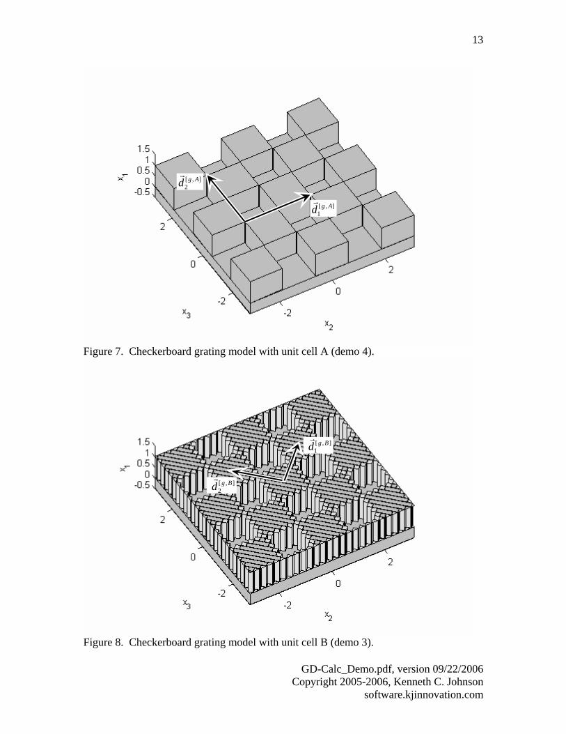
In setting up a biperiodic grating geometry, each biperiodic stratum is defined by partitioning the stratum into stripes parallel to the stratum’s second period vector ( ],[

2Bgd

r

in demo 3, and ],[2

Agdr

in demo 4), and then partitioning each stripe into homogeneous, rectangular structural blocks. This type of block-structured geometry naturally fits the grating configuration with unit cell A, as illustrated in Figure 7; but the diagonal orientation of unit cell B requires that the grating be partitioned into a large number of stripes that approximate the grating walls by sawtooth profiles, as illustrated in Figure 8. (For the purpose of illustration 10 stripes per period are shown in Figure 8, although demo 3 actually uses 1000. The light-shaded blocks in Figure 8 straddle the grating walls, and the permittivity within each of these blocks is defined to be the geometric mean of the grating’s actual permittivity within the block.)



13

],[2

Agdr

],[1

Agdr

Figure 7. Checkerboard grating model with unit cell A (demo 4).

],[1

Bgdr

],[2

Bgdr

Figure 8. Checkerboard grating model with unit cell B (demo 3).



14

The stripe partitioning of grating strata introduces an artificial asymmetry into the mathematical model of the grating, which does not exist in the physical structure; and this asymmetry is reflected in the calculated diffraction efficiencies. For example, one would expect that under normal incidence the order-(1, 0) efficiency (using cell-B order indexing, ( , )) for either or polarization would match the order-(0, 1) efficiency for the same polarization, which it does with unit cell A but not with cell B. On the other hand, one would also expect that the order-(1, 0) efficiency would be the same for both polarizations, which it is with cell B but not with cell A. However, the cell-A symmetry error is an order of magnitude smaller than that of cell B because the grating geometry naturally conforms to the block-structured model description with cell A. Thus, while it is generally desirable to use a unit cell of minimum area (e.g., cell B) to define the diffraction order selection, it may be advantageous to define the grating structure using a different unit cell (e.g. cell A) that requires very few structural blocks for the geometry specification.

][1

Bm ][2Bm 2e 3e

Figure 9 shows a graph of the order-(1, 0) and (0, 1) efficiencies, computed for a range of values for the order truncation limit m_max. (The total number of diffraction orders is .) Convergence lines are shown for several values of L1, the number of cell-B stripes per period. With

2)12( +m_max12m_max = the cell-A symmetry error is

. The cell-B data exhibits no significant symmetry error if only 10 stripes are used, but the convergent result is clearly in error (by

5105.5 −⋅4105.8 −⋅ ) relative to the cell-A

efficiency value. Using 100 stripes, the cell-B result is much more consistent with cell A, but there is a symmetry error of 4107.3 −⋅ . Increasing the number of stripes to 1000 without also increasing m_max does not provide any benefit – it only increases the symmetry error (to ). This is clearly a manifestation of the same kind of problem that occurs when non-lamellar profiles are modeled with high stratification numbers: The electromagnetic field exhibits large spikes inside the “teeth” of the cell-B grating walls, and the field’s Fourier expansion does not have sufficient spatial sampling density to resolve these spikes unless m_max is increased in proportion to L2.

4109.9 −⋅

The symmetry errors can be significantly affected by the diffraction order truncation method. The above example uses simple rectangular truncation, in which and both range from –m_max to +m_max. Figure 10 illustrates the symmetry error using an alternative “diagonal truncation” method in which the sum of || and

is limited in to m_max. With this method, the convergence is less monotonic but the cell-B symmetry error with L2 = 1000 is greatly reduced (and is virtually eliminated when m_max is odd). Also, for a specified m_max limit the total number of diffraction orders is reduced by almost a factor of 2 by using diagonal truncation, cutting computation time by about a factor of 8. (The “alt_order” flags in gdc_demo3.m and gdc_demo4.m can be toggled to use this alternate order truncation.)

][1

Bm][

2Bm

][1

Bm|| ][

2Bm



15

Figure 9. Convergence and stripe-induced symmetry error for checkerboard grating. The legend indicates the unit cell (A or B), the incident polarization direction ( or ), the diffraction order ( ][ , ][ ) relative to cell B, and the number of cell-B stripes per period (L2). Rectangular order truncation is used ( , ).

2e 3e 1Bm 2

Bmm_max≤|| ][

1Bm m_max≤|| ][

2Bm



16

Figure 10. Same as Figure 9, but using diagonal order truncation ( ). m_max≤+ |||| ][

2][

1BB mm



17

Demo 5: Biperiodic grating comprising circular pillars Demo 5 models a grating structure comprising circular pillars centered at the points of an equilateral triangle array, as illustrated in Figure 11. For the purpose of illustration Figure 11 shows nine stripes per pillar, although demo 5 actually uses 1999. (The block partitioning of the circular structures is done with the aid of the utility function circle_partition.m, which is documented in Appendix B.) The grating’s period vectors are designated as ][

1gd

r and ][

2gd

r in Figure 11. The plane of incidence is parallel to

the vector ][2

][1

gg ddrr

+ , and the incident beam is linearly polarized in the plane of incidence, so the diffraction geometry is symmetric with respect to reflection across the incidence plane. The diffraction orders are selected using a hexagonal order truncation scheme of the type illustrated in GD-Calc.pdf, Figure 5 and equations 4.13 and 4.14. If simple rectangular truncation were to be used the selected orders would depend on the choice of unit cell. For example, with the unit cell defined by the basis vectors ][

1gd

r and ][

2gd

r the

index orders ( , ) would be defined by the truncation conditions ,

. Using the cell defined by the basis vectors 1m 2m m_max≤|| 1m

m_max≤|| 2m ][1

gdr

and ][2

][1

gg ddrr

− the truncation conditions would be m_max≤|| 1m , m_max≤− || 21 mm ; and with basis

vectors ][2

gdr

and ][2

][1

gg ddrr

− they would be m_max≤|| 2m , m_max≤− || 21 mm . Demo 5 uses the intersection of these three selection sets to limit ( , ), i.e. the truncation conditions are

1m 2mm_max≤|| 1m , m_max≤|| 2m , m_max≤− || 21 mm .

As with demo 3 and demo 4 the stripe partitioning of the pillars creates small numerical inaccuracies, as evidenced by asymmetries in the calculated diffraction efficiencies. For example, the calculated efficiencies for the (-1, -2) and (-2, -1) transmitted orders are not exactly the same, although one would expect them to be identical based on symmetry. This inconsistency can equivalently be tested in a way that does not rely on symmetry by comparing the order-(-1, -2) efficiencies calculated with the two alternative stripe orientations illustrated in Figures 11 and 12. (In Figure 11 the stripes are parallel to ][

2gd

r, and in Figure 12 they are parallel to ][

1gd

r.) In addition, the

same efficiencies can be computed with the stripe orientation illustrated in Figure 13 (in which the stripe orientation is parallel to ][

2][

1gg dd

rr− ). The Figure 13 configuration

exhibits no symmetry error, but the calculated efficiencies differ slightly from those of Figures 11 and 12. Figure 14 illustrates the results of a convergence and consistency test in which the (-1, -2) transmitted order’s efficiency is plotted versus the order truncation limit m_max for each of the three illustrated stripe orientations, and for several values of the number of stripes per semicircle used to define the pillar geometry. has very little effect on the computation result, but there is a computed effeciency spread of about

between the different stripe orientations (with m_max = 9).

N N

4106.2 −⋅



18

][1

gdr

][2

gdr

incidence plane

Figure 11. Pillar grating of demo 5.

][2

][1

gs ddrr

=

][1

][2

gs ddrr

=

Figure 12. Pillar grating of demo 5 with second stripe orientation.



19

][1

][1

gs ddrr

=][

2][

1][

2ggs ddd

rrr−=

Figure 13. Pillar grating of demo 5 with third stripe orientation. In performing the above test, it is convenient to define the grating geometry in relation to the same grating periods ( ][

1gd

r and ][

2gd

r) and the same coordinate system for

all three stripe orientations so that they can all use the same diffraction order indexing (i.e., index conversions such as equation 18 and 19 are not required); and it is also convenient to use the same incident beam specification for all three configurations. This can be accomplished without having to use different pillar geometry specifications for the different stripe orientations – it is only necessary to change the values of several “harmonic indices” that define a stratum’s periodicity in relation to that of the grating. A stratum is characterized by two fundamental period vectors, ][

1sd

r and ][

2sd

r,

which are typically defined to match to the respective grating periods, ][1

gdr

and ][2

gdr

. However, they may be defined differently, either because the stratum exhibits stronger periodic symmetries than the overall grating, or – as in the case of demo 5 – because it is simply more convenient to use a different set of basis periods to define the stratum. The only limitation in defining the stratum periods is that ][

1gd

r and ][

2gd

r must be linear

combinations of ][1

sdr

and ][2

sdr

with integer linear coefficients, i.e., (26) 1,2

][21,1

][1

][1 hdhdd ssg

rrr+=



20

(27) 2,2][

22,1][

1][

2 hdhdd ssgrrr

+= wherein the ’s (“harmonic indices”) are integers (GD-Calc.pdf, equation 3.18). In other words, the stratum’s basis spatial frequencies

h][

1sf

r and ][

2sf

r must be harmonics of the

grating frequencies ][1

gfr

and ][2

gfr

, (28) ][

22,1][

11,1][

1ggs fhfhf

rrr+=

(29) ][

22,2][

11,2][

2ggs fhfhf

rrr+=

(GD-Calc.pdf, equation 3.31).

Figure 14. Convergence and consistency test for the pillar grating, (-1, -2) transmitted order. The legend indicates which vector is parallel to the stripes ( ][

2gd

r, ][

1gd

r, or

][2

][1

gg ddrr

− ). is the number of stripes per semicircle used to define the pillar geometry. Hexagonal order truncation is used:

Nm_max≤|| 1m , m_max≤|| 2m , . m_max≤− || 12 mm


A stratum’s geometry is specified in relation to its period vectors (as illustrated in GD-Calc.pdf, Figure 3), with the stratum stripes parallel to ][

2sd

r. A linear coordinate

transformation can be implicitly applied to the stratum geometry by changing the


21

definitions of ][1

sdr

and ][2

sdr

, and the definition can also be used to determine the stripe orientation. In the Figure 11 configuration, the stratum periods are simply equated to the respective grating periods: ][

1][

1gs dd

rr= , ][

2][

2gs dd

rr= , so the stripes are parallel to ][

2gd

r. In

Figure 12 the harmonic indices are redefined to swap ][1

sdr

and ][2

sdr

, i.e. ][2

][1

gs ddrr

= , ][

1][

2gs dd

rr= , so the stripes are parallel to ][

1gd

r. In Figure 13, the harmonic indices are set to

define ][1

][1

gs ddrr

= , ][2

][1

][2

ggs dddrrr

−= , so the stripes are parallel to ][2

][1

gg ddrr

− . (The “alt_stripe” selector in gdc_demo5.m controls the branch code that defines the harmonic indices.)

Demo 6 and 7: Biperiodic grating comprising a skewed metal grid Figures 15-18 illustrate the structure modeled by demo 6 and 7, which is a metal grid on a dielectric substrate. Demo 6 models the structure using a unit cell designated as cell A, which is defined by the period vectors ],[

1Agd

r and ],[

2Agd

r. Two stripe orientations

are used, one with the grating stripes parallel to ],[2

Agdr

(Figure 15) or ],[1

Agdr

(Figure 16). Demo 7 uses a different unit cell, designated as cell B, whose defining period vectors

],[1

Bgdr

and ],[2

Bgdr

are ],[

2],[

1],[

1AgAgBg ddd

rrr−= (30)

],[

2],[

1],[

2AgAgBg ddd

rrr+= (31)

Again, two stripe orientations are used, one parallel to ],[

2Bgd

r (Figure 17) and the other

parallel to ],[1

Bgdr

(Figure 18). (The “alt_stripe” selector in gdc_demo6.m and gdc_demo7.m controls the stripe orientation.) Figure 19 illustrates a convergence and consistency test in which the efficiency of the (0, -1) transmitted order (relative to unit cell A) is plotted versus the order truncation limit for the four configurations of Figures 15-18, and for several values of the number

of stripes per grid hole. (Rectangular order truncation is used: , .) Figure 20 illustrates a similar test for the (0, 0) reflected order. For

m_max = 12 the spread of the computed efficiency values is

N m_max≤|| 1mm_max≤|| 2m

4101.7 −⋅ in Figure 19, and in Figure 20. 3104.2 −⋅



22

],[1

Agdr

],[2

Agdr

Figure 15. Metal grid grating with unit cell A (demo 6), first stripe orientation.

],[1

Agdr

],[2

Agdr

Figure 16. Metal grid grating with unit cell A (demo 6), second stripe orientation.



23

],[2

Bgdr

],[1

Bgdr

Figure 17. Metal grid grating with unit cell B (demo 7), first stripe orientation.

],[2

Bgdr

],[1

Bgdr

Figure 18. Metal grid grating with unit cell B (demo 7), second stripe orientation.



24

Figure 19. Convergence and consistency test for metal grid grating of demo 6 and demo 7, (0, -1) transmitted order (relative to unit cell A). The legend indicates which vector is parallel to the stripes ( ],[

2Agd

r, ],[

1Agd

r, ],[

2],[

1AgAg dd

rr+ , or ],[

2],[

1AgAg dd

rr− ). N is the number

of stripes covering each hole.



25

Figure 20. Same as Figure 19, but for the (0, 0) reflected order.



26

Demo 8: Biperiodic grating comprising a square metal grid Figure 21 illustrates the grating structure of demo 8, which is a free-standing, square metal grid illuminated at normal incidence. The and coordinate axes are aligned to the grid, and the grating model’s stripes are parallel to . Figure 22 illustrates a convergence and consistency test for this grating, using one of the first reflected diffraction orders.

2x 3x

3e

Figure 21. Square metal grid grating of demo 8.

Figure 22. Convergence and consistency test for demo 8. The legend indicates the incident polarization direction ( or ) and reflected diffraction order. 3e 2e



27

Demo 9: Alignment sensor This demo models an alignment sensor, which senses small lateral displacements between two proximate grating elements by comparing the intensities of the +1st and –1st-order diffracted beams generated by the gratings. Figure 23 illustrates the grating configuration. Normally-incident illumination passes through an upper transmission grating, reflects off of a lower reflection grating, and passes again through the upper grating, generating +1st and –1st diffraction orders whose relative intensity depends on the gratings’ lateral displacement. (The upper grating’s superstrate, which is modeled as a semi-infinite dielectric medium, is not shown in Figure 23.) A plot of the computed alignment signals as a function of the lateral displacement 2x∆ between upper and lower grating centers is illustrated in Figure 24.

transmission grating

Figure 23. Alignment sensor.

Figure 24. Alignment sensor’s order- unpolarized) as a function of lateral displa

1m

for a particular air space, . 2t

2x∆

reflection grating

dx /2∆

2t

diffraction efficiency (incident field cement 2x∆ (ratioed to the grating period ), d



28

The GD-Calc interface defines a special stratum type that represents a coordinate break, which is used to define the lateral displacement of the top grating element in demo 9. The coordinate break is abstractly classified as a “stratum” of zero thickness, in the sense that it is associated with a lateral plane at a particular height in the grating, and it has the effect of applying a specified lateral ( , ) translational shift to all strata above the coordinate break.

1x

2x 3x

The system illustrated in Figure 23 is represented in the demo script as a multilayer grating structure comprising four strata: (1) the reflection grating stratum, (2) the air gap (of thickness ), (3) the coordinate break (with translational shift ), and (4) the transmission grating stratum. The top grating stratum has a period half that of the bottom grating stratum, so it is specified with a harmonic index of 2, i.e. the top stratum’s fundamental spatial frequency is twice that of the overall grating structure. (Only two harmonic indices, and , are defined for a uniperiodic stratum – in this case

and for the top stratum – because the stratum is characterized by a

single frequency vector

2t 2x∆

1,1h 2,1h21,1 =h 02,1 =h

][1

sfr

; cf. equation 28.) Demo 9 illustrates the parameterization capabilities of GD-Calc. Quantities that are identified as “parameters” in the interface specification (see gdc.m comment header) can, in general, be numeric arrays of any dimensionality. Parameters must all be size-matched, except that a parameter’s singleton dimensions are implicitly repmat-extended to match parameter dimensions. Typically, each parameter dimension is associated with a scalar variable. For example, in demo 9 the air space is defined as a size-[3, 1] column vector (t2=wavelength*[3;2;1]) and the lateral shift

2t

2x∆ is defined as a size-[1, 64] row vector (dx2=d*(0:63)/64). In the GD-Calc internal calculations, all numeric quantities that depend on , but not 2t 2x∆ , will be size-[3, 1] column vectors; all that depend on , but not , will be size-[1, 64] row vectors; and any that depend on both

and will be size-[3, 64] arrays. In particular, the diffraction efficiency arrays returned by gdc_eff will generally be size-[3, 64], as implied by the description of the efficiency outputs as “parameters” in gdc_eff.m. (Zero efficiency values may be represented as scalar zeros, but the values can be expanded to size-[3, 64] arrays via repmat-extension of singleton dimensions.)

2x∆ 2t

2t 2x∆

The repmat-extension convention outlined above can be conceptually viewed as a generalization of MATLAB’s conventions for mixed array-scalar operations. MATLAB generally requires that arguments of array operations such as +, –, etc. be size-matched, e.g. the expression [1,2]+[3;4] will cause an error. However, scalar arguments are implicitly repmat-extended, as required, to match sizes. The expression [1,2]+3, for example, is implicitly interpreted as [1,2]+[3,3]. Under the repmat-extension convention any singleton dimensions may be extended to match sizes, so the expression [1,2]+[3;4] would be implicitly interpreted as [1,2;1,2]+[3,3;4,4].



29

To further illustrate how parameterization can be used, consider the following excerpt from gdc_demo2.m, which defines the incident E

r field,

wavelength=1.533; phi=30*pi/180; psi=45*pi/180; ... inc_field.wavelength=wavelength; inc_field.f2=sin(phi)*cos(psi)/wavelength; inc_field.f3=sin(phi)*sin(psi)/wavelength; This code could be modified to do a wavelength and directional scan of the incident beam, with wavelength vectorized in dimension 3 and direction vectorized in dimension 4. The following code illustrates how this could be done, wavelength=shiftdim([1.4,1.5,1.6],-1); phi=shiftdim([0,30,30,30,60,60,60]*pi/180,-2); psi=shiftdim([0,15,30,45,15,30,45]*pi/180,-2); ... inc_field.wavelength=wavelength; size3=size(wavelength); size4=size(phi); inc_field.f2=... repmat(sin(phi).*cos(psi),size3)./repmat(wavelength,size4); inc_field.f3=... repmat(sin(phi).*sin(psi),size3)./repmat(wavelength,size4); In this example, wavelength is size-[1, 1, 3], the polar and azimuth incident angles (phi and psi) are size-[1, 1, 1, 7], and the f2 and f3 parameters are size-[1, 1, 3, 7] (because they are functions of both wavelength and incidence direction). Repmat extension is applied explicitly in defining f2 and f3. Parameterization can, in some instances, considerably improve computation runtime, but it can also considerably increase memory requirements. Therefore parameterization should be used judiciously on complex, memory-intensive problems, such as biperiodic gratings, to get the most performance benefit within the limitation of memory resources. Parameterizing the incident field (wavelength and incidence angles) will generally provide no significant performance benefit, so in the above example from demo 2, parameterization would only be used as a convenience. However, demo 9 illustrates a situation in which parameterization greatly improves runtime performance. To see how it does so, it helps to understand a little about how the GD-Calc internal algorithms work. The GD-Calc calculations are primarily based on two operations: first, calculating an “S matrix” (scattering matrix) for each individual stratum in the grating; and second, combining the S matrices for the strata by means of a “stacking” operation, which is applied from bottom to top to determine a cumulative S matrix for the entire grating. In demo 9 there are parameter combinations in total (3 air spacings and 64 lateral displacements), so if the and

192643 =×2t 2x∆ parameters were iterated outside gdc.m, all of



30

these S matrix computations would have to be repeated 192 times. But if vectorized parameters are used the S matrices for the grating strata will only be calculated once (because they have no dependence on or 2t 2x∆ ), the S matrix for the air space (which depends only on ) will be calculated only 3 times, and the S matrix for the coordinate break (which depends only on ) will only be calculated 64 times. Furthermore, the air space stacking operation will only be calculated 3 times; and only the stacking operations above the air space must be repeated for all 192 parameter combinations.

2t

2x∆

Generally, parameter vectorization may be most effective when applied to parameters that only affect the uppermost grating strata, because this will avoid redundant stacking operations for lower strata. Thus, for complex, resource-intensive applications a good strategy would be to first try vectorizing parameters for the top strata, and if you don’t get a memory error then try vectorizing parameters associated with lower strata. The plotting routine, gdc_plot.m, is designed to work with parameterized grating structures. The second gdc_plot argument is a multidimensional parameter index, which specifies which parameter combination is to be plotted. The demo 9 code illustrates how the plotting function can be used to generate a simple animation showing a parameter scan of . 2x∆

Demo10: Slanted lamellar grating The grating structure modeled by demo 10 is illustrated in Figure 25. The structure is a slanted lamellar grating designed to operate as a Bragg deflector for an EUV wavelength of 11 nm. (This grating geometry approximates the peripheral portion of a high-NA, diffractive EUV microlens.) The grating is configured for optimum efficiency in the second diffraction order, and Figure 26 illustrates the 2nd-order efficiency as a function of wavelength. The slanted lamellae are approximated as a stack of thin, unslanted lamellar grating strata. For the purpose of illustration eight strata are illustrated in Figure 25, although demo 10 actually uses 32. The lateral offset between strata is represented by a coordinate break, similar to that described in the preceding demo-9 discussion. Rather than explicitly defining 32 separate lamellar strata and associated coordinate breaks, demo 10 uses a “replication module” to implicitly stack 32 copies of a structure comprising just one lamellar stratum and one coordinate break. The advantage of using a replication module is not just one of convenience: Whereas the computation runtime would generally be proportional to the number of strata, with a replication module the runtime is only proportional to the logarithm of the number of strata. Thus, a very large number of very thin strata can be used without incurring a significant increase in runtime.



31

Demo 10 also illustrates the use of published refractive index data (e.g. for ruthenium and diamond-like carbon). See the utility function read_nk.m for additional information on material data.

Figure 25. EUV Bragg diffraction grating of demo 10.

Figure 26. EUV grating’s Bragg diffraction efficiency in the 2nd diffraction order for unpolarized, normally-incident illumination.



32

Demo 11: Crossed-line grating The structure modeled by demo 11 (see Figure 27) is a photonic crystal comprising a stack of crossed, uniperiodic grating layers, each layer comprising square-section tungsten rods. (Refractive index data for tungsten is obtained from the file W.nk using the accessory function, read_nk.m.) For this example diagonal order truncation is used. Figure 28 illustrates convergence plots comparing the performance of diagonal truncation ( ) and rectangular truncation ( ,

). The two methods exhibit similar convergence performance, but computation time is reduced by about a factor of 8 using diagonal truncation. Figure 29 illustrates the grating’s computed zero-order reflectance and transmittance spectra for several values of the order truncation limit m_max.

m_max≤+ |||| ][2

][1

BB mm m_max≤|| ][1

Bmm_max≤|| ][

2Bm

The demo 11 code only computes the efficiency at one wavelength. Wavelength vectorization is not recommended for this type of structure due to the high number of diffraction orders. The Figure 29 data was generated by iterating wavelength in an outer loop, using 201 uniformly-spaced reciprocal-wavelength values.

Figure 27. Tungsten photonic crystal (demo 11). The grating structure is represented as a replication module comprising the following three stratum elements (from bottom to top): (1) a uniperiodic stratum with the grating lines in the direction, (2) a uniperiodic stratum with the grating lines in the 3x 2x



33

direction, and (3) a coordinate break, which applies a half-period translational shift in both the and directions. (The second uniperiodic stratum is constructed by simply swapping the harmonic indices of the first stratum.) The replication count (rep_count) is 4, giving a total of 8 uniperiodic grating strata. (The computation time scales in proportion to log(rep_count), so much deeper structures could be easily analyzed.)

2x 3x

Figure 28. Convergence test for tungsten photonic crystal (zero-order reflectance for unpolarized, normally-incident illumination at wavelength m825.1 µ ). Two order truncation methods are compared: rectangular truncation ( m_max|| 1 ≤m , ) and diagonal truncation (

m_max|| 2 ≤mm_max|||| 21 ≤+ mm ).

reflectance

transmittance

Figure 29. Computed zero-order reflectance and transmittance spectra for the tungsten photonic crystal, with unpolarized, normally-incident illumination, using diagonal order truncation.



34

Appendix A: Interface for gdc_demo_engine.p The generic interface for gdc_demo_engine is [grating,param_size,scat_field,inc_field]=... gdc_demo_engine(demo_sel,inc_field,order,varargin) demo_sel is an integer in the range of 1 to 11 that selects which demo to run. The inc_field and order inputs and the param_size, scat_field and inc_field outputs are as documented in gdc.m. Also, the grating output corresponds to the first gdc.m input argument. The main difference between gdc_demo_engine and gdc is that the grating struct is not an input, but is constructed internally by gdc_demo_engine based on several demo-specific inputs (the “varargin” inputs). These inputs are outlined below. (See the demo code examples for more detailed description of arguments and usage examples.) Demo 1: uniperiodic, sinusoidal grating [grating,param_size,scat_field,inc_field]=... gdc_demo_engine(1,inc_field,order,... grating_pmt,d,h,L1,ctr_sect); grating_pmt: grating permittivity d: grating period h: grating height L1: number of strata ctr_sect: option for center-sectioning strata (true or false) Demo 2: biperiodic grating comprising rectangular pyramids [grating,param_size,scat_field,inc_field]=... gdc_demo_engine(2,inc_field,order,... grating_pmt,d1,d2,h,L1); grating_pmt: grating permittivity d1, d2: grating periods h: grating height L1: number of strata



35

Demo3: biperiodic checkerboard grating, unit cell B [grating,param_size,scat_field,inc_field]=... gdc_demo_engine(3,inc_field,order,... grating_pmt,w,h,L2); grating_pmt: grating permittivity w: width of squares h: grating height L2: number of stripes (must be even) Demo4: biperiodic checkerboard grating, unit cell A [grating,param_size,scat_field,inc_field]=... gdc_demo_engine(4,inc_field,order,... grating_pmt,w,h); grating_pmt: grating permittivity w: width of squares h: grating height Demo 5: biperiodic grating comprising circular pillars [grating,param_size,scat_field,inc_field]=... gdc_demo_engine(5,inc_field,order,... grating_pmt,d,h,r,N,alt_stripe); grating_pmt: grating permittivity d: grating period h: grating height r: pillar radius N: number of partition blocks per semicircle (for pillars) alt_stripe: selector for alternate stripe orientation (1, 2, or 3) Demo 6: biperiodic grating – skewed metal grid, unit cell A [grating,param_size,scat_field,inc_field]=... gdc_demo_engine(6,inc_field,order,... substrate_pmt,stratum_pmt,d,h,N,alt_stripe); substrate_pmt: substrate permittivity stratum_pmt: stratum permittivity d: grating period h: grating height N: number of partition stripes covering each hole alt_stripe: selector for alternate stripe orientation (1 or 2)



36

Demo 7: biperiodic grating – skewed metal grid, unit cell B [grating,param_size,scat_field,inc_field]=... gdc_demo_engine(7,inc_field,order,... substrate_pmt,stratum_pmt,d,h,N,alt_stripe); substrate_pmt: substrate permittivity stratum_pmt: stratum permittivity d: grating period h: grating height N: number of "teeth" on each edge of the hole alt_stripe: selector for alternate stripe orientation (1 or 2) Demo 8: biperiodic grating - square metal grid [grating,param_size,scat_field,inc_field]=... gdc_demo_engine(8,inc_field,order,... stratum_pmt,d,h,c); stratum_pmt: stratum permittivity d: grating period h: grating height c: hole width/period Demo 9: alignment sensor [grating,param_size,scat_field,inc_field]=... gdc_demo_engine(9,inc_field,order,... substrate_pmt,superstrate_pmt,d,t1,t2,t3,dx2); substrate_pmt: substrate permittivity superstrate_pmt: superstrate (phase plate) permittivity d: grating period t1: bottom (reflecting) grating thickness t2: air space thickness t3: phase plate grating thickness dx2: phase plate's lateral shift



37

Demo 10: slanted lamellar grating [grating,param_size,scat_field,inc_field]=... gdc_demo_engine(10,inc_field,order,... sub_pmt,film_pmt,grating_pmt,... d,t1,t2,rep_count,wall_t,slant); sub_pmt: substrate permittivity film_pmt: base film permittivity grating_pmt: grating layer permittivity d: grating period t1: base film thickness t2: grating layer thickness rep_count: replication count wall_t: grating wall thickness slant: slant angle of grating walls (radians) Demo 11: crossed-line grating [grating,param_size,scat_field,inc_field]=... gdc_demo_engine(11,inc_field,order,... grating_pmt,d,thick,width,rep_count); grating_pmt: grating permittivity d: grating period thick: stratum thickness width: grating line width rep_count: replication count

Appendix B. Algorithm notes for circle_partition.m Figure B1 illustrates a unit circle whose first quadrant is partitioned into blocks, e.g. in Figure B1. The geometry is defined so that the shaded regions between the circle and the block profile all have the same area, denoted below as

N4=N

A . The block geometry is characterized in terms of the angles 1θ , 2θ , … N2θ at which the block profile intercepts the circle, and the angle sequence is constrained to have the following reversal symmetry, jNj −+−= 122 θθ π (B1) The bottommost shaded region straddles two quadrants, and its area is ]cos[]sin[ 111 θθθ −=A (B2)



38

An analysis of the Figure B1 geometry yields the following relationship between successive intercept angles,

⎪⎩

⎪⎨⎧

−++−−−+−

=++++

++++

even),(])sin[]cos[]sin[](cos[]sin[]cos[odd),(])sin[]cos[]sin[](cos[]sin[]cos[

1111

1111

21

21

21

21

jj

Ajjjjjjjj

jjjjjjjj

θθθθθθθθθθθθθθθθ

(B3) This implicitly represents a recursion relation defining 1+jθ from jθ . (Newton’s method is used to solve for 1+jθ .) The recursion is iterated for Nj K1= , and the initial angle 1θ is iteratively adjusted until the following terminal condition is satisfied: 12 +−= NN θθ π (B4) (from equation B1).

5θ

4θ

3θ

2θ

1θ

6θ7θ

8θ Figure B1. Block-partitioned circle geometry ( 4=N ).



39

The 1θ iteration is initialized by making small-angle approximations in equation B3. For 11 <<−+ jj θθ , the following approximation is obtained, 2

1 )(]2sin[41

jjjA θθθ −≅ + (B5) The angle difference jj θθ −+1 can be approximated as a derivative,

djd

jjθθθ ≅−+1 (B6)

This results in the following approximation for j as a function of θ ,

∫+≅j

dA

jθ

θθθ

1 4]2sin[1 (B7)

The sine term is further approximated as θθ 2]2sin[ ≅ (B8) so that equation B7 reduces to

( 2/31

2/32311 θθ −+≅ jA

j ) (B9)

Hence,

3/2

2/312

3)1( ⎟⎟⎠

⎞⎜⎜⎝

⎛+−≅ θθ Ajj (B10)

The relationship between 1θ and A defined by equation B2 can be approximated as 3

132θ≅A (B11)

This substitution reduces equation B10 to

( ) 1

3/213)1( θθ +−≅ jj (B12)

Equation B4 implies the following approximate equivalence,



40

42/1πθ ≅+N (B13)

Equations B12 and B13 yield the following initial approximation for 1θ ,

( 3/221

4 13)(1

−+−≅ Nπθ ) (B14)

With this initialization, Newton’s method (with a finite-difference derivative estimator) is used to eliminate the error in relation B4 by successive refinement of the 1θ estimate.



gd calc demo

Documents