gauss–jordan elimination method for computing outer inverses

Applied Mathematics and Computation 219 (2013) 4667–4679

Contents lists available at SciVerse ScienceDirect

Applied Mathematics and Computation

journal homepage: www.elsevier .com/ locate/amc

Gauss–Jordan elimination method for computing outer inverses q

Predrag S. Stanimirovic ⇑, Marko D. PetkovicUniversity of Niš, Faculty of Sciences and Mathematics, Višegradska 33, 18000 Niš, Serbia

a r t i c l e i n f o a b s t r a c t

Keywords:Gauss–Jordan eliminationGeneralized inverseouter inverse

0096-3003/$ - see front matter � 2012 Elsevier Inchttp://dx.doi.org/10.1016/j.amc.2012.10.081

q Authors gratefully acknowledge support from th⇑ Corresponding author.

E-mail addresses: [email protected] (P.S. Stanim

This paper deals with the algorithm for computing outer inverse with prescribed range andnull space, based on the choice of an appropriate matrix G and Gauss–Jordan elimination ofthe augmented matrix ½GjI�. The advantage of such algorithms is the fact that one can com-pute various generalized inverses using the same procedure, for different input matrices. Inparticular, we derive representations of the Moore–Penrose inverse, the weighted Moore–Penrose inverse, the Drazin inverse as well as f2;4g and f2;3g-inverses. Numerical exam-ples on different test matrices are presented, as well as the comparison with well–knownmethods for generalized inverses computation.

� 2012 Elsevier Inc. All rights reserved.

1. Introduction

Using the usual notation, by Cm�nr we denote the set of all complex m� n matrices of rank r, and by I we denote the unit

matrix of an appropriate order. Furthermore A�; RðAÞ; rankðAÞ andNðAÞ denote the conjugate transpose, the range, the rankand the null space of A 2 Cm�n.

If A 2 Cm�nr ; T is a subspace of Cn of dimension t 6 r and S is a subspace of Cm of dimension m� t, then A has a f2g-inverse

X such that RðXÞ ¼ T and NðXÞ ¼ S if and only if AT � S ¼ Cm. In the case when the existence is ensured, X is unique and it is

denoted by Að2ÞT;S. Outer generalized inverses with prescribed range and null-space are very important in matrix theory. Theyare used in constructing iterative methods for solving nonlinear equations [1,8] as well as in statistics [4,5]. Furthermore,outer inverses play an important role in stable approximations of ill-posed problems and in linear and nonlinear problemsinvolving rank-deficient generalized inverses [7,19]. Observing from the theoretical point of view, it is well known that the

Moore–Penrose inverse and the weighted Moore–Penrose inverse Ay;AyM;N , the Drazin and the group inverse AD;A#, as well as

the Bott-Duffin inverse Að�1ÞðLÞ and the generalized Bott-Duffin inverse AðyÞðLÞ can be presented by a unified approach, as general-

ized inverses Að2ÞT;S for appropriate choice of matrices T and S. For example, the next statements are valid for a rectangular ma-trix A (see [1,9,16]):

Ay ¼ Að2ÞRðA�Þ;NðA�Þ; AyM;N ¼ Að2ÞRðA]Þ;NðA]Þ; ð1:1Þ

where M;N are positive definite matrices of appropriate orders and A] ¼ N�1A�M. For a given square matrix A the next iden-tities are satisfied (see [1–3,16]):

AD ¼ Að2ÞRðAkÞ;NðAkÞ

; A# ¼ Að2ÞRðAÞ;NðAÞ; ð1:2Þ

. All rights reserved.

e Research Project 174013 of the Serbian Ministry of Science.

irovic), [email protected] (M.D. Petkovic).

http://dx.doi.org/10.1016/j.amc.2012.10.081

mailto:[email protected]

mailto:[email protected]

http://dx.doi.org/10.1016/j.amc.2012.10.081

http://www.sciencedirect.com/science/journal/00963003

http://www.elsevier.com/locate/amc

4668 P.S. Stanimirovic, M.D. Petkovic / Applied Mathematics and Computation 219 (2013) 4667–4679

where k ¼ indðAÞ. If A is the L-positive semi–definite matrix and L is a subspace of Cn which satisfiesAL� L? ¼ Cn, S ¼ RðPLAÞ, then the next identities are satisfied (see [2,16,17]):

Að�1ÞðLÞ ¼ Að2Þ

L;L?; AðyÞðLÞ ¼ Að2Þ

S;S?: ð1:3Þ

We study Gauss–Jordan elimination methods for computing various outer inverses of complex matrices. The oldest and bestknown among these methods is the method for calculating the inverse matrix. The Gauss–Jordan elimination method forcomputing the inverse of a nonsingular matrix A is based on the executing elementary row operations on the pair A j I½ �and its transformation into the block matrix IjA�1

h iinvolving the inverse A�1. A number of numerical methods are developed

for computing various classes of outer inverses with prescribed range and null space. The Gauss–Jordan elimination methodto compute the Moore–Penrose inverse is developed in [12]. The method from [12] is based on two successive sets of ele-mentary row operations. The first computes reduced row echelon form of A�A:

E A�A j I½ � ¼E1A�A E1

O E2

� �ð1:4Þ

while the second provides the following transformation

E1A�A E1

E2 O

� �! I

E1A�AE2

� ��1�� E1

O

� �" #:

After that, Moore–Penrose inverse can be computed by

Ay ¼E1A�A

E2

� ��1 E1

O

� �A�:

More general algorithm for computing Að2ÞT;S inverses is introduced in [13]. This algorithm is very useful generalization of themethod from [12]. The essence of this generalization consists in the replacement of the matrix A� by an appropriate matrix G.

Several improvements of the algorithm from [12] are recently presented in [6]. First improvement from [6] assumes theinitial transformation of the form

E A�jI½ � ¼E1A� E1

O E2

� �:

The second improvement exploits special structure of the matrix which is subject in Gauss–Jordan transformation.Two main goals of the present paper should be emphasized.Firstly, motivated by the modification introduced in [6], in the present paper we introduce corresponding modification of

the algorithm introduced in [13]. This possibility is mentioned in the conclusion of the paper [6]. That type algorithms areable to compute various generalized inverses of matrix A, for different choice of an input matrix G.

Moreover, we observed that the algorithms introduced in [6,12,13] are not accompanied by adequate implementationand not tested on adequate test examples. The numerical properties of these algorithms are not studied in details so far.Our second goal is the implementation of described algorithms and the numerical experience derived applying theimplementation.

The paper is organized as follows. Necessary preliminary results are surveyed in the next section. Our main algorithm isdefined in the third section after necessary theoretical investigations. In Section 4 we presented an illustrative numericalexample and explain our motivation for the corresponding improvements of the algorithm. These improvements save thecomputational time and increase numerical stability of the main algorithm. Exploiting our implementation in the program-ming language C++, in the last section we tested considered algorithms on randomly generated test matrices. Also, a series ofnumerical experiments corresponding to the Moore–Penrose inverse and the Drazin inverse are presented.

2. Preliminary results

There exist a number of full–rank representations for outer inverses of prescribed rank as well as for outer inverses withprescribed range and kernel. The following representations from [11,18] will be useful for our results that follow.

Proposition 2.1. Let A 2 Cm�nr ; T be a subspace of Cn of dimension s 6 r and let S be a subspace of Cm of dimension m� s. In

addition, suppose that G 2 Cn�m satisfies RðGÞ ¼ T;NðGÞ ¼ S. Let G has an arbitrary full–rank decomposition, that is G ¼ UV. If Ahas a f2g-inverse Að2ÞT;S, then:

(1) [11] VAU is an invertible matrix and

Að2ÞT;S ¼ UðVAUÞ�1V ¼ Að2ÞRðUÞ;NðVÞ: ð2:1Þ

(2) [18] indðAGÞ ¼ indðGAÞ ¼ 1 and

P.S. Stanimirovic, M.D. Petkovic / Applied Mathematics and Computation 219 (2013) 4667–4679 4669

Að2ÞT;S ¼ GðAGÞ# ¼ ðGAÞ#G: ð2:2Þ

According to known representations from [1,10,11,14,15] we state the next additional representations withrespect to (1.1)–(1.3). These representations characterize the classes of f2g; f2;4g and f2;3g generalized inverses ofknown rank.

Proposition 2.2. Let A 2 Cm�nr be an arbitrary matrix and let 0 < s 6 r be a positive integer. The following general representations

for some classes of generalized inverses are valid:

(a) Af2gs ¼ fAð2ÞRðUÞ;NðVÞ ¼ UðVAUÞ�1V jU 2 Cn�s; V 2 Cs�m; rankðVAUÞ ¼ sg;

(b) Af2;4gs ¼ Að2;4ÞRððVAÞ�Þ;NðVÞ ¼ ðVAÞ� VAðVAÞ�ð Þ�1V jV 2 Cs�ms

n o¼ ðVAÞyV jVA 2 Cs�n

s

n o;

(c) Af2;3gs ¼ Að2;3ÞRðUÞ;NððAUÞ�Þ ¼ U ðAUÞ�AUð Þ�1ðAUÞ�jU 2 Cn�ss

n o¼ UðAUÞyjAU 2 Cm�s

s

n o;

(d) Af1;2g ¼ Af2gr :

Sheng and Chen in [13] derived the following representation of the Að2ÞT;S inverse corresponding to a particular choice of thematrix G

Að2ÞT;S ¼E1GA

E2

� ��1 E1

O

� �G; ð2:3Þ

where matrices E1 and E2 are defined by elementary row operations

E GAjI½ � ¼E1GA E1

O E2

� �: ð2:4Þ

The authors of the paper [13] derive an explicit expression for the group inverse ðGAÞ# and later, using this representation(2.2), established the representation (2.3).

Sheng and Chen in [13] also proposed the following Gauss–Jordan elimination algorithm for calculating the representa-tion (2.3):

Algorithm 2.1. Computing the Að2ÞT;S inverse of the matrix A using the Gauss–Jordan elimination. (Algorithm GJATS2)

Require: Matrix A 2 Cm�nr and matrix G 2 Cn�m

s where s 6 r.1: Execute elementary row operations (2.4) on the pair ½GAjI�.2: Exchange the block of zeros with the corresponding block of the lower right–hand of the above 2� 2 block

matrix, then resuming elementary row operations on the pair

E1GA E1

E2 O

� �

to transform it into

I j Y½ � ¼ IE1GA

E2

� ��1�� E1

O

� �" #:

3: Compute the output

Að2ÞRðGÞ;NðGÞ ¼E1GA

E2

� ��1 E1

O

� �G ¼ YG:

The particular case G ¼ A� the representation (2.3) produces analogous representation of the Moore–Penrose inverse andAlgorithm 2.1 reduces to the corresponding algorithm for computing the Moore–Penrose inverse. This representation andalgorithm are proposed in [12]. Corresponding algorithm we denote by Algorithm GJMP.

On the other hand, the following improvement of Algorithm GJMP is recently published in [6]:


Algorithm 2.2. Computing the Ay using the Gauss–Jordan elimination. (Algorithm GJMP1)

Require: The matrix A of dimensions m� n and of rank r.1: Execute elementary row operations on the pair ½A�jI� to get the reduced row echelon form

E A�jI½ � ¼E1A� E1

O E2

� �¼

B E1

O E2

� �;

where the notation B ¼ E1A� is used.2: Compute BA and form

BA B

E2 O

� �


I�� Ay

h i¼ I

�� BA

E2

� ��1 B

O

� �" #:

3: Return the output

Ay ¼BAE2

� ��1 BO

� �:

Our goal in the present paper is to improve Algorithm GJATS2 in the same way as Algorithm GJMP1 improves AlgorithmGJMP. That gives a coherent set of numerical methods of similar type, which numerical properties are are also examined.

3. The algorithm

We start by proving the main theorem, which gives the representation of Að2ÞT;S inverse corresponding to matrix G, using theincomplete Gauss–Jordan elimination of the matrix ½GjI�.

Theorem 3.1. Let A 2 Cm�nr is given matrix. Let G 2 Cn�m

s is given matrix satisfying 0 < s 6 r. Assume that the conditionAT � S ¼ Cm is satisfied in the case T ¼ RðGÞ; S ¼ NðGÞ. Let

E1G

O

� �¼

B

O

� �

be the reduced row echelon form of G and E is the product of all elementary matrices corresponding to s pivoting steps of Gauss–Jordan elimination on GjI½ �, satisfying

E GjI½ � ¼B E1

O E2

� �:

Then the matrix

BA

E2

� �ð3:1Þ

is nonsingular and

Að2ÞRðGÞ;NðGÞ ¼BA

E2

� ��1 B

O

� �¼

E1GA

E2

� ��1 E1G

O

� �: ð3:2Þ

Proof. Denote the first s rows of E by E1. By E2 we denote the remaining n� s columns of E. It follows that

EG ¼E1

E2

� �G ¼

E1G

O

� �¼

B

O

� �; ð3:3Þ

where the notation B ¼ E1G is used for the sake of simplification. We also have

E2G ¼ O;

which implies RðGÞ � N ðE2Þ. Due to the fact


dimðN ðE2ÞÞ þ dimðRðE2ÞÞ ¼ dimðN ðE2ÞÞ þ rankðE2Þ ¼ n

and rankðE2Þ ¼ n� s we have

dimðN ðE2ÞÞ ¼ n� ðn� sÞ ¼ s ¼ rankðGÞ ¼ dimðRðGÞÞ;

and later

NðE2Þ ¼ RðGÞ: ð3:4Þ

Since the identity RðGÞ ¼ T holds, we have

NðE2Þ ¼ RðGÞ ¼ RðAð2ÞT;SÞ;

which further implies

E2Að2ÞT;S ¼ O: ð3:5Þ

On the other hand, the following holds:

BAAð2ÞT;S ¼ B:

Indeed, if G ¼ UV is a full–rank factorization of G, according to Proposition 2.1 we obtain

Að2ÞT;S ¼ UðVAUÞ�1V

and

BAAð2ÞT;S ¼ E1ðUVÞAUðVAUÞ�1V ¼ E1UV ¼ E1G ¼ B:

The last identity in conjunction with (3.5) implies

BA

E2

� �Að2ÞT;S ¼

B

O

� �: ð3:6Þ

In order to complete the proof it is necessary to verify invertibility of the matrix

BA

E2

� �:

Let x 2 Cn satisfy

E1GAE2

� �x ¼ 0:

Then immediately follows E2x ¼ E1GAx ¼ 0. The condition E2x ¼ 0 implies

x 2 NðE2Þ ¼ RðGÞ ¼ RðGAÞ: ð3:7Þ

From E1GAx ¼ 0, taking into account (3.4), we derive

x 2 NðE1GAÞ ¼ N ðGAÞ: ð3:8Þ

According to assertions (3.7) and (3.8) and Proposition 2.1 we have

x 2 RðGAÞ \ N ðGAÞ ¼ f0g ) x ¼ 0; ð3:9Þ

which completes the proof. h

According to the representation introduced in Theorem 3.1, we introduce the following algorithm for computing Að2ÞT;S

inverses:


Algorithm 3.1. Computing the Að2ÞT;S using the Gauss–Jordan elimination. (Algorithm GJATS2PM)

Require Matrix A 2 Cm�nr and matrix G 2 Cn�m

s where s 6 r.1: Perform elementary row operations on the pair ½GjI� to get the reduced row echelon form

E G j I½ � ¼E1G E1

O E2

� �¼

B E1

O E2

� �:

2: Compute BA and form the block matrix

BA B

E2 O

� �:

Transform this matrix into

I�� X

h i¼ I

�� BA

E2

� ��1 B

O

� �" #

applying the Gauss–Jordan elimination3: Return

Að2ÞRðGÞ;NðGÞ ¼ X ¼BA

E2

� ��1 B

O

� �:

It is possible to use Algorithm GJATS2PM to compute the common six important generalized inverses, for different choices ofinput matrices.

Corollary 3.1. For a given matrix A 2 Cm�nr and arbitrarily chosen matrix G 2 Cn�m

s the following statements are valid for thegeneralized inverse Að2ÞRðGÞ;NðGÞ produced by Algorithm GJATS2PM:

E1GA

E2

� ��1 E1G

O

� �¼ Að2ÞRðGÞ;NðGÞ ¼

Ay; G ¼ A�;

AyM;N; G ¼ A];

AD; G ¼ Al

; l P indðAÞ;A#; G ¼ A;

Að�1ÞðLÞ ; RðGÞ ¼ L; NðGÞ ¼ L?;

AðyÞðLÞ; RðGÞ ¼ S; NðGÞ ¼ S?:

8>>>>>>>>>><>>>>>>>>>>:

ð3:10Þ

Furthermore, using representations from [15], we derive Gauss–Jordan elimination methods for generating f2g; f2;4g andf2;3g–inverses.

Corollary 3.2. Let A 2 Cm�nr be the given matrix, s 6 r be a given integer. Assume that the conditions of Theorem 3.1 are satisfied.

Then the following statements are valid:

(a) If G ¼ UV is arbitrary full-rank factorization of G, then expression (3.2) produces

E1GAE2

� ��1 E1GO

� �¼ Að2ÞRðUÞ;NðVÞ ¼ UðVAUÞ�1V 2 Af2gs: ð3:11Þ

(b) In the case G ¼ ðVAÞ�V 2 Cn�ms expression (3.2) produces

E1GA

E2

� ��1 E1G

O

� �¼ Að2;4ÞRððVAÞ�Þ;NðVÞ ¼ ðVAÞ�ðVAðVAÞ�Þ�1V ¼ ðVAÞyV 2 Af2;4gs: ð3:12Þ

(c) In the case G ¼ UðAUÞ� 2 Cn�ms the following holds:

E1GA

E2

� ��1 E1G

O

� �¼ Að2;3ÞRðUÞ;NððAUÞ�Þ ¼ UððAUÞ�AUÞ�1ðAUÞ� ¼ UðAUÞy 2 Af2;3gs: ð3:13Þ

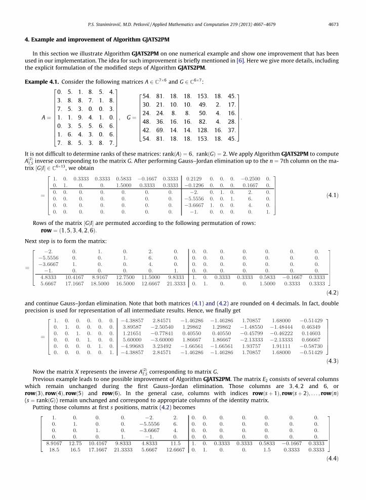
4. Example and improvement of Algorithm GJATS2PM

In this section we illustrate Algorithm GJATS2PM on one numerical example and show one improvement that has beenused in our implementation. The idea for such improvement is briefly mentioned in [6]. Here we give more details, includingthe explicit formulation of the modified steps of Algorithm GJATS2PM.

Example 4.1. Consider the following matrices A 2 C7�6 and G 2 C6�7:


A ¼

0: 5: 1: 8: 5: 4:3: 8: 8: 7: 1: 8:7: 5: 3: 0: 0: 3:1: 1: 9: 4: 1: 0:0: 3: 5: 5: 6: 6:1: 6: 4: 3: 0: 6:7: 8: 5: 3: 8: 7:

2666666666664

3777777777775; G ¼

54: 81: 18: 18: 153: 18: 45:30: 21: 10: 10: 49: 2: 17:24: 24: 8: 8: 50: 4: 16:48: 36: 16: 16: 82: 4: 28:42: 69: 14: 14: 128: 16: 37:54: 81: 18: 18: 153: 18: 45:

2666666664

3777777775:

It is not difficult to determine ranks of these matrices: rankðAÞ ¼ 6; rankðGÞ ¼ 2. We apply Algorithm GJATS2PM to computeAð2ÞT;S inverse corresponding to the matrix G. After performing Gauss–Jordan elimination up to the n ¼ 7th column on the ma-trix ½GjI� 2 C6�13, we obtain

ð4:1Þ

Rows of the matrix ½GjI� are permuted according to the following permutation of rows:
row ¼ ð1;5;3;4;2;6Þ:
Next step is to form the matrix:

ð4:2Þ

and continue Gauss–Jordan elimination. Note that both matrices (4.1) and (4.2) are rounded on 4 decimals. In fact, doubleprecision is used for representation of all intermediate results. Hence, we finally get

ð4:3Þ

Now the matrix X represents the inverse Að2ÞT;S corresponding to matrix G.Previous example leads to one possible improvement of Algorithm GJATS2PM. The matrix E2 consists of several columns

which remain unchanged during the first Gauss–Jordan elimination. Those columns are 3;4;2 and 6, orrowð3Þ; rowð4Þ; rowð5Þ and rowð6Þ. In the general case, columns with indices rowðsþ 1Þ; rowðsþ 2Þ; . . . ; rowðnÞ(s ¼ rankðGÞ) remain unchanged and correspond to appropriate columns of the identity matrix.

Putting those columns at first s positions, matrix (4.2) becomes

ð4:4Þ


Choosing the main diagonal elements as pivots, in the first n� r ¼ 4 steps of Gauss–Jordan elimination, we significantlyreduce the number of required arithmetic operations. That is since we do not need to update a submatrix consisting of thefirst n� r ¼ 4 rows and columns of the matrix (4.2). Continuing Gauss–Jordan elimination on the matrix (4.4) we obtain thesame matrix X (as in (4.3), but with permuted rows, according to the permutation ðrowðsþ 1Þ; rowðsþ 2Þ; . . . ;

rowðnÞ; rowð1Þ; rowð2Þ; . . . ; rowðsÞÞ as we used for columns of the matrix (4.2).Shown idea can be used for all input matrices A and G. For a matrix M 2 Cm�n and appropriate permutations p and q, de-

note by Mp;� and M�;q matrices formed by permutation of rows and columns according to permutations p and q respectively.Assume that

row ¼ ðrowð1Þ; rowð2Þ; . . . ; rowðnÞÞ

is the permutation of rows obtained during Gauss–Jordan elimination procedure. Since there is no pivot element belong torows rowðsþ 1Þ; rowðsþ 2Þ; . . . ; rowðnÞ, columns of the matrix I (in initial matrix ½GjI�) with the same indices are unchangedduring the elimination process. Consider the permutation of columns

col ¼ ðrowðsþ 1Þ; rowðsþ 2Þ; . . . ; rowðnÞ; rowð1Þ; rowð2Þ; . . . ; rowðsÞÞ

and form

ðE2Þ�;col O

ðBAÞ�;col B

" #: ð4:5Þ

The first s rows and columns of the matrix (4.5) form the identity matrix Is�s. Hence, by choosing the first r main diagonalelements as pivot elements in second Gauss–Jordan elimination, only last n� r rows and nþm� r columns of matrix (4.5)need to be updated in each step. After the elimination is done, the final matrix has the form ½Ij~X�, where ~X ¼ Xcol;�. Now, ma-trix X is easily computed by applying the row permutation col�1 on the matrix ~X, i.e. X ¼ ~Xcol�1 ;�.

According to the above discussion, we can formulate the following improvement of Algorithm GJATS2PM.

Algorithm 4.1. Improved algorithm for computing the Að2ÞT;S using the Gauss–Jordan elimination. (AlgorithmGJATS2PMimp)

Require Matrix A 2 Cm�nr and matrix G 2 Cn�m

s where s 6 r.1: Execute elementary row operations on the pair ½Gj I� to get the reduced row echelon form

E G j I½ � ¼E1G E1

O E2

� �¼

B E1

O E2

� �:

During the elimination, maintain the permutation of rows row ¼ ðrowð1Þ; rowð2Þ; . . . ; rowðnÞÞ.2: Form the permutation of columns

col ¼ ðrowðr þ 1Þ; rowðr þ 2Þ; . . . ; rowðnÞ; rowð1Þ; rowð2Þ; . . . ; rowðrÞÞ:

3: Compute BA and form

ðE2Þ�;col O

ðBAÞ�;col B

" #;


I j ~Xh i

¼ IðE2Þ�;col

ðBAÞ�;col

" #�1��

O

B

� �24

35:

4: Compute col�1 and return

Að2ÞRðGÞ;NðGÞ ¼ X ¼ ~Xcol�1 ;�:

Note that, in the same way, we can construct an improvement of Algorithm GJATS2, which will be denoted by AlgorithmGJATS2imp.

5. Numerical experiments

It is realistic to expect that two successive applications Gauss–Jordan elimination procedures contribute to bad condition-ing of numerical algorithms. We implemented Algorithm GJATS2imp and Algorithm GJATS2PMimp in programming lan-guage C++ and tested on randomly generated test matrices. Note that papers [12,13], where Algorithm GJATS2 is


introduced, does not contain any numerical experiments. The same situation is in the paper [6] of J. Ji introducing the specialcase of Algorithm GJATS2PM for computing Moore–Penrose inverse Ay of matrix A. Hence, in this paper, we provide testingresults for both Algorithm GJATS2imp and GJATS2PMimp. Those results include the special cases of Moore–Penrose andDrazin inverse, obtained for the choice G ¼ A� and G ¼ Ak (k ¼ indðAÞ ¼ minfl 2 NjrankðAlþ1Þ ¼ rankðAlÞg), respectively. Inthe case of Moore–Penrose inverse, we compared our algorithms with Matlab function pinv which implements well-knownSVD (Singular Value Decomposition) method.

Code is compiled by Microsoft Visual Studio 2010 compiler with default compiler settings. All generated matriceshad unit norm, but different values of rank.

Furthermore, we list the following two more issues we used in the implementation of both Algorithm GJATS2imp andAlgorithm GJATS2PMimp:

1. While performing Gauss–Jordan elimination, we first select non-zero entries in pivot row and column and update onlythose fields contained in the cross product of those entries. This improvement is based on the fact that (in both algo-rithms) Gauss–Jordan elimination is applied on matrices containing non-negligible number of zero elements.

2. Note that the matrix B in Algorithm GJATS2PMimp has exactly s unit columns and others have at least n� s zeros. Thisfact can be used to significantly reduce the number of operations (also running time) needed to compute product ofmatrices B and A. In other words, we can reduce the number of multiplications to

Table 1Maxima

n

(a) T300350400450500550600650700

(b) T300350400450500550600650700

#fbij j bij – 0; i ¼ 1;2; . . . ; s; j ¼ 1;2; . . . ;mg n:

where B ¼ ½bij�16i6s;16j6n. Similar fact can be used for the last step of Algorithm GJATS2imp.

5.1. Numerical experiments for the Moore–Penrose inverse

In the case G ¼ A� the resulting matrix X is the Moore–Penrose inverse Ay of the matrix A. Tables 1 and 2 show maximalerror norms for matrices A 2 Cn�n with rankðAÞ ¼ n=2 and rankðAÞ ¼ 10, obtained for 20 different randomly generated testmatrices.

We see that both algorithms give satisfactory results, while Algorithm GJATS2PMimp is better, average by 3 orders ofmagnitude.

Average running times of our algorithms and pinv function from Matlab are shown in Table 3. Testings are done on IntelCore-i5 720 processor (without multi-core optimization) with 4 GB of RAM. All presented times are in seconds and obtainedby averaging times on 20 test matrices.

It can be seen that Algorithm GJATS2PMimp outperforms Algorithm GJATS2imp in all test cases. One possible reason forsuch behavior is the fact that Algorithm GJATS2imp needs to compute the product A�A (i.e. GA), where both A� and A are notsparse.

In the case of low-rank matrices (rankðAÞ ¼ 10) we see that Algorithm GJATS2PMimp also outperforms pinv, while forrankðAÞ ¼ n=10 results are comparable each to other. In the case rankðAÞ ¼ n=2, both algorithms are slower than pinv.

According to the above discussion, we can conclude that Algorithm GJATS2PMimp is the best choice for computing Ay oflow-rank matrices.

l error norms of the result of Algorithm GJATS2imp, on random matrices.

kAXA� Ak kXAX � Xk kAX � ðAXÞTk kXA� ðXAÞTk

he case rankðAÞ ¼ n=23.339e�008 8.835e�007 3.479e�009 1.172e�0084.155e�008 1.899e�007 2.561e�009 8.668e�0081.531e�007 2.844e�007 3.897e�009 1.318e�0077.013e�008 1.515e�007 2.070e�009 3.073e�0073.199e�007 4.253e�007 5.348e�009 1.273e�0072.713e�008 6.711e�007 7.852e�009 7.348e�0071.622e�008 5.577e�007 1.707e�009 1.281e�0073.644e�007 1.374e�006 1.419e�008 4.342e�0073.764e�006 1.515e�006 1.525e�008 2.146e�006

he case rankðAÞ ¼ 104.382e�012 2.216e�013 2.963e�013 4.002e�0121.160e�012 1.299e�013 1.242e�013 4.003e�0121.943e�012 1.423e�013 1.669e�013 3.319e�0122.237e�012 1.864e�013 1.811e�013 2.992e�0124.140e�012 1.571e�013 2.347e�013 4.421e�0121.003e�011 1.584e�013 1.215e�012 8.514e�0125.490e�012 2.536e�013 1.455e�012 2.307e�0111.577e�012 1.985e�013 3.212e�013 4.745e�0121.122e�011 2.997e�013 4.213e�013 3.457e�012

Table 2Maximal error norms of the result of Algorithm GJATS2PMimp, on random matrices.

n kAXA� Ak kXAX � Xk kAX � ðAXÞTk kXA� ðXAÞTk

(a) The case rankðAÞ ¼ n=2300 5.275e�012 5.035e�010 3.298e�011 2.654e�011350 1.276e�011 4.166e�008 1.030e�009 1.028e�009400 4.204e�012 2.215e�009 5.602e�011 5.719e�011450 1.057e�011 1.944e�008 4.954e�010 4.769e�010500 9.138e�012 3.988e�008 8.342e�010 8.623e�010550 6.269e�012 1.736e�009 3.723e�011 3.704e�011600 1.647e�012 4.279e�009 1.160e�010 1.286e�010650 3.299e�011 1.964e�007 3.558e�009 4.000e�009700 8.328e�010 3.680e�009 1.370e�009 1.505e�009

(b) The case rank ðAÞ ¼ 10300 1.938e�012 3.021e�015 1.016e�013 1.130e�013350 1.397e�012 1.141e�015 5.099e�014 5.784e�014400 1.279e�012 8.597e�016 4.093e�014 4.293e�014450 2.930e�012 1.793e�015 9.655e�014 8.348e�014500 1.117e�011 5.935e�015 3.084e�013 3.239e�013550 2.989e�011 1.118e�014 7.070e�013 8.488e�013600 3.423e�012 8.750e�016 7.263e�014 9.354e�014650 4.555e�012 1.192e�015 9.920e�014 1.026e�013700 8.849e�012 2.323e�015 2.003e�013 2.069e�013

Table 3Comparison of the running times for Matlab function pinv, Algorithm GJATS2imp and Algorithm GJATS2PMimp. All times are in seconds.

n pinv GJATS2imp GJATS2PMimp

rankðAÞ ¼ 10300 0.016 0.040 0.006350 0.022 0.064 0.008400 0.031 0.092 0.011450 0.044 0.128 0.015500 0.057 0.173 0.020550 0.082 0.235 0.023600 0.098 0.293 0.026650 0.122 0.373 0.032700 0.128 0.461 0.037

rankðAÞ ¼ n=10300 0.019 0.048 0.014350 0.023 0.076 0.020400 0.032 0.111 0.030450 0.043 0.158 0.047500 0.056 0.217 0.060550 0.071 0.288 0.079600 0.112 0.377 0.101650 0.130 0.472 0.129700 0.144 0.592 0.164

rankðAÞ ¼ n=2.300 0.022 0.097 0.057350 0.030 0.151 0.089400 0.043 0.226 0.131450 0.059 0.319 0.185500 0.075 0.439 0.263550 0.096 0.584 0.343600 0.124 0.761 0.434650 0.148 0.953 0.551700 0.172 1.198 0.701


5.2. Numerical experiments for the Drazin inverse

Algorithms GJATS2imp and GJATS2PMimp are tested in the case G ¼ Ak (k ¼ indA) where the result matrix X is Drazininverse AD of the matrix A. Running times, as well as the residual vectors are shown in Tables 4 and 5.

Numerical results show that Algorithm GJATS2PMimp also outperformed Algorithm GJATS2imp both in the result accu-racy and running time. Especially this is the case for low-rank matrices where Algorithm GJATS2PMimp gives the bestperformance.

Table 4Running times and maximal error norms of the result of Algorithm GJATS2PMimp for random matrices.

n Running time [s] kAkþ1X � Akk kXAX � Xk kAX � XAk

(a) Case rankðAÞ ¼ n=2300 0.056 4.666e�007 7.661e�003 1.789e�005350 0.086 1.578e�008 5.237e�005 1.408e�007400 0.129 9.349e�007 8.507e�003 2.957e�006450 0.183 5.138e�007 4.327e�002 2.154e�005500 0.256 2.154e�007 1.033e�002 1.856e�005550 0.332 9.233e�007 5.782e�004 5.745e�007600 0.425 4.101e�007 1.576e�001 2.103e�005650 0.541 9.463e�008 7.659e�004 4.400e�007700 0.698 7.869e�008 6.755e�004 1.282e�006

(b) Case rankðAÞ ¼ 10.300 0.006 2.501e�011 6.186e�009 3.357e�010350 0.009 5.713e�009 2.125e�006 9.657e�008400 0.011 2.912e�010 3.992e�008 1.641e�009450 0.015 3.037e�010 3.718e�008 1.238e�009500 0.018 2.923e�010 5.487e�008 2.038e�009550 0.022 4.160e�010 2.910e�007 2.062e�009600 0.027 1.570e�008 2.142e�006 3.913e�008650 0.032 2.424e�010 1.584e�007 7.107e�009700 0.038 7.359e�010 1.463e�006 1.697e�008

Table 5Running times and maximal error norms of the result of Algorithm GJATS2imp for random matrices.

n Running time [s] kAkþ1X � Akk kXAX � Xk kAX � XAk

(a) Case rankðAÞ ¼ n=2300 0.097 7.519e�006 5.708e�003 6.331e�005350 0.149 1.248e�006 1.432e�003 1.364e�005400 0.222 1.011e�005 8.619e�002 1.722e�005450 0.326 1.233e�005 1.792e�003 6.304e�005500 0.438 2.347e�005 7.228e�003 8.896e�005550 0.591 4.670e�005 1.400e�003 4.472e�004600 0.759 5.907e�005 4.975e�003 1.184e�005650 0.947 4.620e�006 7.662e�002 2.380e�004700 1.202 2.145e�006 1.836e�003 4.503e�004

(b) Case rankðAÞ ¼ 10300 0.041 1.840e�010 5.096e�009 9.251e�010350 0.063 5.626e�010 9.591e�008 6.579e�009400 0.091 1.853e�009 5.527e�007 7.432e�009450 0.133 7.938e�010 1.233e�007 3.885e�009500 0.177 4.871e�010 3.989e�008 3.767e�009550 0.230 4.396e�009 2.045e�007 8.048e�008600 0.305 2.577e�009 4.200e�007 3.045e�008650 0.393 1.755e�009 1.126e�007 1.384e�008700 0.462 8.892e�009 7.409e�007 6.244e�008


5.3. Numerical experiments for randomly generated matrix G

Finally, we show numerical results in the case when both matrices A and G are chosen randomly. In such case, obtainedmatrix X is only f2g inverse of A and therefore, we only show the norm of kXAX � Xk. At it can be seen from Tables 6–8, Algo-rithm GJATS2PMimp clearly outperforms Algorithm GJATS2imp in all test cases. Both algorithms have smaller running timesfor matrices with lower rank. It is worth noting that accuracy also depends on the rank of both A and G and it is drasticallyreduced when rankðAÞ rankðGÞ.

6. Conclusions

Two main objectives are achieved in the present paper. First, we define several improvements of the algorithm forgenerating the outer inverses with prescribed range and null space from [13]. Our improvements follow corresponding

Table 6Running times and maximal error norms of results of Algorithms GJATS2imp and GJATS2PMimp for randomly generated matrices A and G with rankðAÞ ¼ n andrankðGÞ ¼ n=2.

n GJATS2imp GJATS2PMimp

Running time [s] kXAX � Xk Running time [s] kXAX � Xk

300 0.095 8.364e�009 0.057 1.073e�010350 0.151 1.169e�008 0.087 4.560e�010400 0.226 2.719e�009 0.129 1.203e�010450 0.312 2.186e�007 0.185 1.071e�010500 0.439 7.630e�001 0.262 6.420e�010550 0.602 6.427e�008 0.334 3.717e�010600 0.738 3.383e�005 0.431 1.117e�006650 0.941 1.953e�008 0.578 9.035e�010700 1.192 3.983e�008 0.719 3.476e�010

Table 7Running times and maximal error norms of results of Algorithms GJATS2imp and GJATS2PMimp for randomly generated matrices A and G with rankðAÞ ¼ n=2and rankðGÞ ¼ 10.



300 0.039 8.936e�007 0.006 3.939e�006350 0.063 8.309e�006 0.008 6.899e�007400 0.094 1.868e�007 0.012 1.113e�006450 0.129 2.835e�007 0.015 8.278e�007500 0.175 8.142e�008 0.020 4.975e�008550 0.230 2.054e�007 0.023 3.943e�007600 0.294 4.490e�007 0.023 5.761e�007650 0.385 1.708e�006 0.036 2.072e�007700 0.460 4.150e�007 0.040 3.417e�006

Table 8Running times and maximal error norms of results of Algorithms GJATS2imp and GJATS2PMimp for randomly generated matrices A and G with rankðAÞ ¼ n=2and rankðGÞ ¼ n=2.



300 0.096 1.074e�001 0.056 4.654e�003350 0.151 2.426e�003 0.087 1.641e�005400 0.225 7.318e�002 0.130 1.077e�003450 0.317 1.130e+000 0.204 3.251e�003500 0.440 2.739e�001 0.295 2.423e�002550 0.587 1.085e+001 0.364 4.872e�001600 0.738 6.261e+000 0.469 3.024e�001650 0.943 1.383e+000 0.603 3.619e�002700 1.190 4.178e�001 0.739 1.240e�001


modifications of the algorithm from [12], which are presented in [6]. In this way, our paper represents a continuation of re-sults given in [6,11–13]. Defined algorithm represents an another algorithm for computing outer inverses with prescribedrange and null space as well as an algorithm based on the Gauss–Jordan elimination procedure.

In addition, the paper presents a numerical study on the properties of algorithms based on the Gauss–Jordan eliminationand aimed in computation of generalized inverses. For this purpose, we give a set of numerical examples to compare thesealgorithms with several well–known methods for computing the Moore–Penrose inverse and the Drazin inverse.

In this paper we searched for the answer to the important question: how good are methods based on two Gauss–Jordaneliminations? Our numerical experience indicates that the answer depends on the type of inverse which is being computedand the rank of both matrices A and G:

� In the case of the Moore–Penrose inverse (G ¼ A�), methods are stable and fast for low-rank matrices A. Both running timeand accuracy are degraded for higher rank matrices.


� In the case of the Drazin inverse (G ¼ Ak; k ¼ indðAÞ), running times are similar to the previous case, while accuracy is

more reduced with increase of rankðAÞ.� Finally, in the general case of arbitrary A and G, we also see that better results are obtained in cases when rankðGÞ is small,

while accuracy is reduced when rankðAÞ rankðGÞ.

Hence, methods based on Gauss–Jordan elimination are most practically applicable as a unique tool for computation of arbi-trary low–rank generalized inverses of matrix A.

References

[1] A. Ben-Israel, T.N.E. Greville, Generalized Inverses: Theory and Applications, second ed., Springer, 2003.[2] Y. Chen, The generalized Bott–Duffin inverse and its application, Linear Algebra Appl. 134 (1990) 71–91.[3] R.E. Cline, Inverses of rank invariant powers of a matrix, SIAM J. Numer. Anal. 5 (1968) 182–197.[4] A.J. Getson, F.C. Hsuan, f2g-Inverses and their statistical, applications, Lecture Notes in Statistics, vol. 47, Springer, Berlin, 1988.[5] F. Husen, P. Langenberg, A. Getson, The {2}-inverse with applications to satistics, Linear Algebra Appl. 70 (1985) 241–248.[6] J. Ji, Gauss–Jordan elimination methods for the Moore–Penrose inverse of a matrix, Linear Algebra Appl. 437 (2012) 1835–1844.[7] M.Z. Nashed, Generalized Inverse and Applications, Academic Press, New York, 1976.[8] M.Z. Nashed, X. Chen, Convergence of Newton-like methods for singular operator equations using outer inverses, Numer. Math. 66 (1993) 235–257.[9] R. Piziak, P.L. Odell, Full rank factorization of matrices, Math. Mag. 72 (1999) 193–201.

[10] C.R. Rao, S.K. Mitra, Generalized Inverse of Matrices and its Applications, John Wiley & Sons, Inc., New York, London, Sydney, Toronto, 1971.[11] X. Sheng, G. Chen, Full–rank representation of generalized inverse Að2ÞT;S and its applications, Comput. Math. Appl. 54 (2007) 1422–1430.[12] X. Sheng, G.L. Chen, A note of computation for M–P inverse Ay , Int. J. Comput. Math. 87 (2010) 2235–2241.[13] X. Sheng, G.L. Chen, Y. Gong, The representation and computation of generalized inverse Að2ÞT;S , J. Comput. Appl. Math. 213 (2008) 248–257.[14] P.S. Stanimirovic, Block representations of f2g; f1;2g inverses and the Drazin inverse, Indian J. Pure Appl. Math. 29 (1998) 1159–1176.[15] P.S. Stanimirovic, D.S. Cvetkovic-Ilic, S. Miljkovic, M. Miladinovic, Full-rank representations of f2;4g; f2;3g-inverses and successive matrix squaring

algorithm, Appl. Math. Comput. 217 (2011) 9358–9367.[16] G. Wang, Y. Wei, S. Qiao, Generalized Inverses: Theory and Computations, Science Press, Beijing/New York, 2004.[17] Y. Wei, H. Wu, The representation, The representation and approximation for the generalized inverse Að2ÞT;S , Appl. Math. Comput. 135 (2003) 263–276.[18] Y. Wei, A characterization and representation of the generalized inverse Að2ÞT;S and its applications, Linear Algebra Appl. 280 (1998) 79–86.[19] B. Zheng, R.B. Bapat, Generalized inverse Að2ÞT;S and a rank equation, Appl. Math. Comput. 155 (2) (2004) 407–415.

gauss–jordan elimination method for computing outer inverses

Documents