Sandia National Laboratories is a multimission laboratory managed and operated by National Technology and Engineering Solutions of Sandia, LLC, a wholly

owned subsidiary of Honeywell International Inc., for the U.S. Department of Energy’s National Nuclear Security Administration under contract DE-NA0003525.

Gaussian Process Models

Laura Swiler

Uncertainty Quantification Summer School

Sponsored by the DOE FASTMATH Institute and USC

Aug. 14-16, 2019

SAND2019-9565C

Acknowledgments

▪ Summer School on the Design and Analysis of Computer Experiments, Aug. 2006. Part of a SAMSI Program, taught in part by Jerry Sacks and Will Welch.

▪ John McFarland (now at Southwest Research Institute) ▪ Dissertation: UNCERTAINTY ANALYSIS FOR COMPUTER SIMULATIONS

THROUGH VALIDATION AND CALIBRATION. Vanderbilt University, 2008.

▪ Discussions with Tony O’Hagan (University of Sheffield) over the years.

▪ Many Sandians, including Brian Rutherford, Patty Hough, Brian Adams, Mike Eldred, John Jakeman, Cosmin Safta, Ari Frankel, and Keith Dalbey.

▪ Discussions with Brian Williams and Dave Higdon at Los Alamos.

▪ Many others: thank you!

2

Overview

▪ Metamodels

▪ Gaussian Process background

▪ Gaussian Process formulation

▪ Different views of Gaussian processes

▪ Examples

▪ Use of Gaussian Processes within other methods (e.g. optimization, calibration)

▪ Constrained GPs

▪ Efficient methods for constructing GPs

3

Metamodels

▪ Metamodels: also called surrogate, response surface model, or emulator.

▪ Typically constructed over a small number of simulation model runs (“code runs”)

▪ The simulation is very costly to run, we can only afford a limited number of runs, often dozens to a few hundred

▪ The code runs provide the training data (e.g. sets of input parameters and corresponding response values)

▪ The metamodel is constructed to provide a fast, cheap function evaluation for the purposes of uncertainty quantification, sensitivity analysis, and optimization.

▪ Simpson, T. W., V. Toropov, V. Balabanov, and F.A.C. Viana. Design and analysis of computer experiments in multidisciplinary design optimization: A review of how far we have come or not. In Proceedings of the 12th AIAA/ISSMO Multidisciplinary Analysis and Optimization Conference), Victoria, British Columbia, Canada, September 2008. AIAA Paper 2008-5802.

4

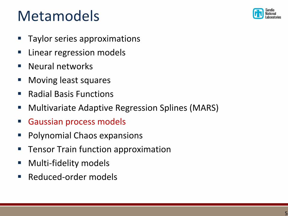
Metamodels

▪ Taylor series approximations

▪ Linear regression models

▪ Neural networks

▪ Moving least squares

▪ Radial Basis Functions

▪ Multivariate Adaptive Regression Splines (MARS)

▪ Gaussian process models

▪ Polynomial Chaos expansions

▪ Tensor Train function approximation

▪ Multi-fidelity models

▪ Reduced-order models

5

Surrogates vs. Machine Learning

▪ Are surrogates and ML the same thing?

▪ I would argue that surrogates are a subset, but in a limited way: ▪ Typically surrogate models are constructed over small data sets

▪ Surrogates typically don’t involve classification, unsupervised data, transfer learning, reinforcement learning, image analysis, text analysis.

▪ Surrogates are function approximations.

▪ Surrogates are an example of supervised learning (both inputs and outputs are provided in the training data).

▪ GPs can be used for regression and classification, both of which are supervised learning.

▪ Recent interest in the intersection of UQ and ML.

6

Shout out to Paul Constantine’s bibliography

7

Paul is curating a bibliography of recent work applying machine learning and related tools to problems in computational science and engineering. Here's the link:

http://www.cs.colorado.edu/~paco3637/sciml-refs.html

• P. A. Romero, A. Krause, and F. H. Arnold. Navigating the protein fitness

landscape with Gaussian processes. Proceedings of the National Academy of

Sciences, 110(3):813--813, 2013. [ bib | http ]

• M. Guo and J. S. Hesthaven. Reduced order modeling for nonlinear structural

analysis using Gaussian process regression. Computer Methods in Applied

Mechanics and Engineering, 341:807--826, 2018. [ bib | http ]

• C. A. Thimmisetty, R. G. Ghanem, J. A. White, and X. Chen. High-dimensional

intrinsic interpolation using Gaussian process regression and diffusion

maps. Mathematical Geosciences, 50(1):77--96, 2018. [ bib | http ]

• M. Raissi, P. Perdikaris, and G. E. Karniadakis. Machine learning of linear

differential equations using Gaussian processes. Journal of Computational

Physics, 348:683--693, 2017. [ bib | http ]

Gaussian Processes

▪ Why are GPs popular emulators of computer models? ▪ They allow modeling of fairly complicated functional forms

▪ They do not just offer a prediction at a new point but an estimate of the uncertainty in that prediction

▪ Classic references: ▪ Sacks, J., W.J. Welch, T.J. Mitchell, and H.P. Wynn. Design and analysis

of computer experiments. Statistical Science, 4(4):409–435, 1989.

▪ Santner, T., B. Williams, and W. Notz. The Design and Analysis of Computer Experiments. New York, NY: Springer, 2003.

▪ Rasmussen, C.E. and C.K.I. Williams. Gaussian Processes for Machine Learning. MIT Press, 2006. e-book:

▪ http://www.gaussianprocess.org/gpml/chapters/

8

Gaussian Process

▪ A stochastic process is a collection of random variables {y(x) | xX} indexed by a set X in d, where d is the number of inputs.

▪ A Gaussian process is a stochastic process for which any finite set of y-variables has a joint multivariate Gaussian distribution. That is, the joint probability distribution for every finite subset of variables y(x1), ..y(xk) is multi-variatenormal.

▪ A GP is fully specified by its mean function (x) = E[y(x)] and its covariance function C(x, x′).

9

What does this mean?

▪ Start with a set of runs of a computer code: at each sample xi

we have output yi(xi).

▪ The output at a new input value, xnew, is uncertain.

▪ This is what a GP will predict: ŷ(xnew).

▪ Related to regression.

▪ Related to random functions. From our set of samples, we have a function that is a set of points {x, y(x)} or {x, f(x)}. Instead of f(x), if we use the outcome of a random draw from some joint distribution of random variables {Z(x1), … Z(xn)}, we get a realization of a random function.

▪ This is a stochastic process (e.g. generate many draws and get many functions).

10

How do we simulate realizations of a random function?

▪ Start with {Z(x1), … Z(xn)} from a multivariate normal distribution with mean 0 and covariance matrix C=Cov[Z(xi), Z(xj)].

▪ To simulate a random draw:

▪ Generate n standard normal(0,1) random variables, S.

▪ Perform a Cholesky decomposition C= LLt.

▪ Define Z = LS.

▪ Plot the points {xi, Zi = Z(xi)}

▪ Connect the dots

11

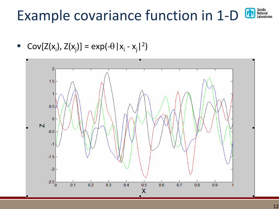
Example covariance function in 1-D

▪ Cov[Z(xi), Z(xj)] = exp(-|xi - xj|2)

12

Gaussian Process

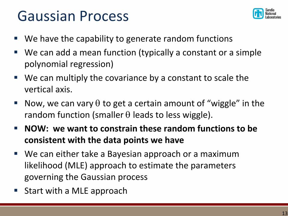
▪ We have the capability to generate random functions

▪ We can add a mean function (typically a constant or a simple polynomial regression)

▪ We can multiply the covariance by a constant to scale the vertical axis.

▪ Now, we can vary to get a certain amount of “wiggle” in the random function (smaller leads to less wiggle).

▪ NOW: we want to constrain these random functions to be consistent with the data points we have

▪ We can either take a Bayesian approach or a maximum likelihood (MLE) approach to estimate the parameters governing the Gaussian process

▪ Start with a MLE approach

13

Gaussian Process

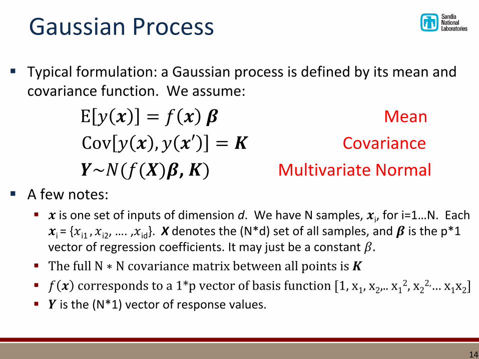
▪ Typical formulation: a Gaussian process is defined by its mean and covariance function. We assume:

E 𝑦 𝒙 = 𝑓 𝒙 𝜷 Mean

Cov 𝑦 𝒙 , 𝑦 𝒙′ = 𝑲 Covariance

𝒀~𝑁(𝑓(𝑿)𝜷, 𝑲) Multivariate Normal

▪ A few notes: ▪ 𝒙 is one set of inputs of dimension d. We have N samples, 𝒙i, for i=1…N. Each

𝒙i = {𝑥i1 , 𝑥i2, …. ,𝑥id}. X denotes the (N*d) set of all samples, and 𝜷 is the p*1 vector of regression coefficients. It may just be a constant 𝛽.

▪ The full N ∗ N covariance matrix between all points is 𝑲

▪ 𝑓 𝒙 corresponds to a 1*p vector of basis function [1, x1, x2,.. x12, x2

2,… x1x2]

▪ 𝒀 is the (N*1) vector of response values.

14

Gaussian Process

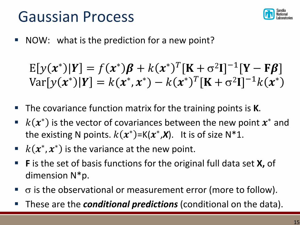
▪ NOW: what is the prediction for a new point?

E 𝑦 𝒙∗ |𝒀 = 𝑓 𝒙∗ 𝜷 + 𝑘 𝒙∗ 𝑇[𝐊 + 2𝐈]−1[𝐘 − 𝐅𝜷]Var[𝑦 𝒙∗ 𝒀 = 𝑘(𝒙∗, 𝒙∗) − 𝑘 𝒙∗ 𝑇[𝐊 + 2𝐈]−1𝑘 𝒙∗

▪ The covariance function matrix for the training points is K.

▪ 𝑘 𝒙∗ is the vector of covariances between the new point 𝒙∗ and the existing N points. 𝑘 𝒙∗ =K(𝒙∗,X). It is of size N*1.

▪ 𝑘 𝒙∗, 𝒙∗ is the variance at the new point.

▪ F is the set of basis functions for the original full data set X, of dimension N*p.

▪ is the observational or measurement error (more to follow).

▪ These are the conditional predictions (conditional on the data).

15

Gaussian Process

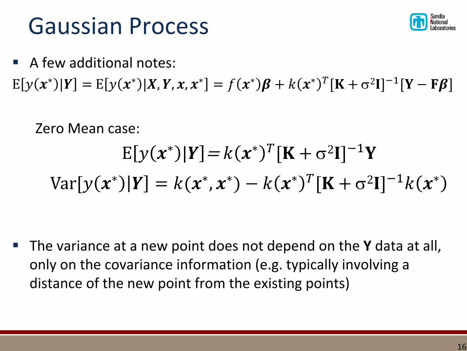
▪ A few additional notes:

E 𝑦 𝒙∗ |𝒀 = E 𝑦 𝒙∗ |𝑿, 𝒀, 𝒙, 𝒙∗ = 𝑓 𝒙∗ 𝜷 + 𝑘 𝒙∗ 𝑇[𝐊 + 2𝐈]−1[𝐘 − 𝐅𝜷]

Zero Mean case:

E 𝑦 𝒙∗ |𝒀 = 𝑘 𝒙∗ 𝑇[𝐊 + 2𝐈]−1𝐘

Var[𝑦 𝒙∗ 𝒀 = 𝑘(𝒙∗, 𝒙∗) − 𝑘 𝒙∗ 𝑇[𝐊 + 2𝐈]−1𝑘 𝒙∗

▪ The variance at a new point does not depend on the Y data at all, only on the covariance information (e.g. typically involving a distance of the new point from the existing points)

16

Gaussian Process

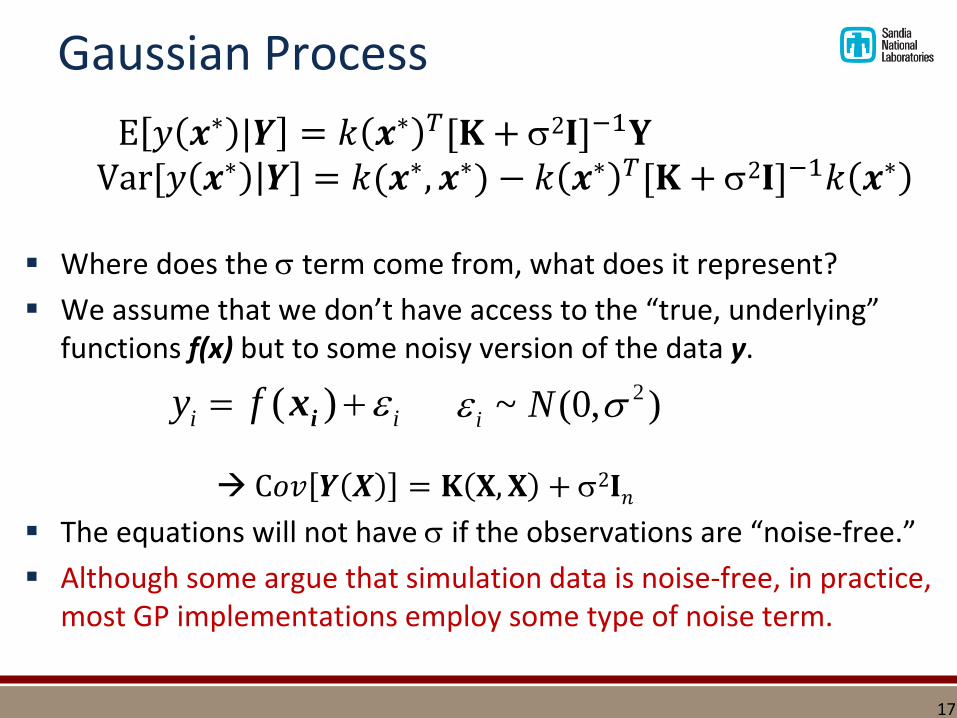
▪ Where does the term come from, what does it represent?

▪ We assume that we don’t have access to the “true, underlying” functions f(x) but to some noisy version of the data y.

C𝑜𝑣 𝒀 𝑿 = 𝐊 𝐗, 𝐗 + 2𝐈𝑛

▪ The equations will not have if the observations are “noise-free.”

▪ Although some argue that simulation data is noise-free, in practice, most GP implementations employ some type of noise term.

E 𝑦 𝒙∗ |𝒀 = 𝑘 𝒙∗ 𝑇[𝐊 + 2𝐈]−1𝐘Var[𝑦 𝒙∗ 𝒀 = 𝑘(𝒙∗, 𝒙∗) − 𝑘 𝒙∗ 𝑇[𝐊 + 2𝐈]−1𝑘 𝒙∗

( )i iy f i

x 2~ (0, )i N

17

What does this look like?

18

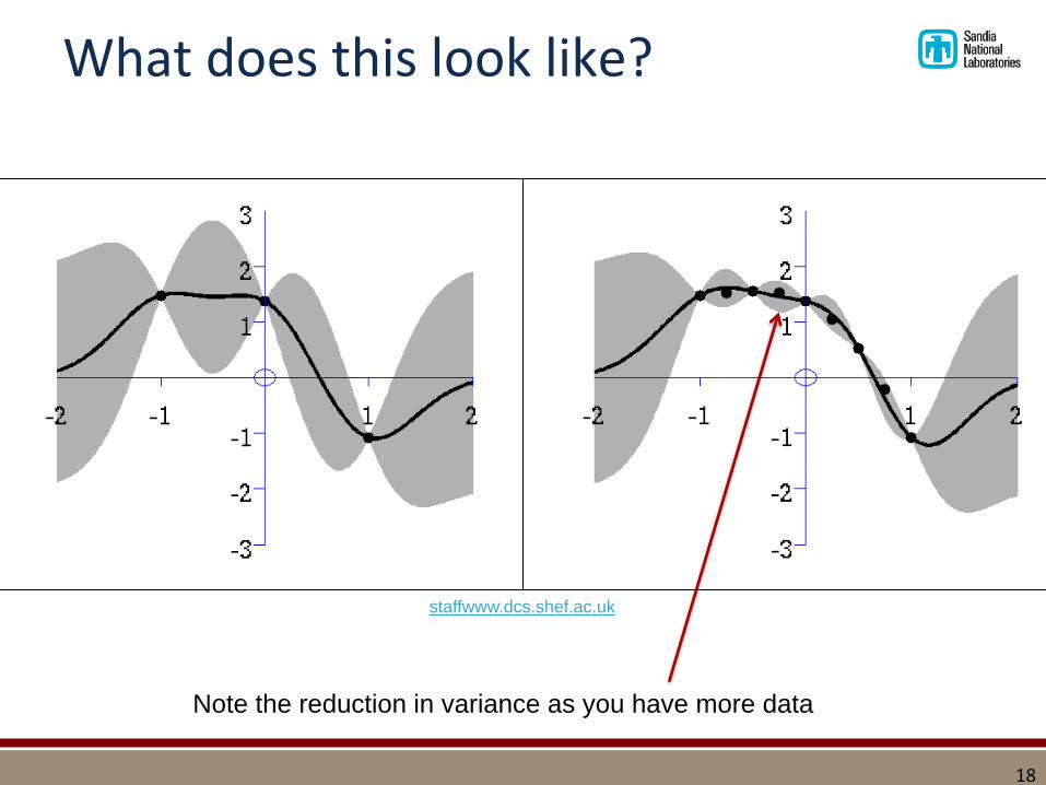
staffwww.dcs.shef.ac.uk

Note the reduction in variance as you have more data

What does this look like?

19

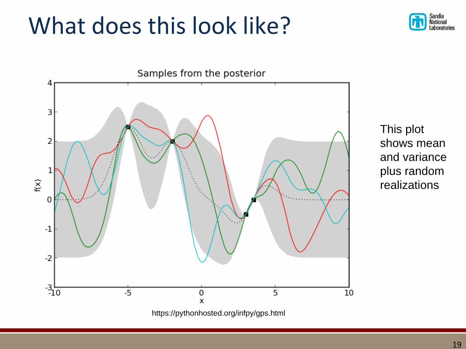
https://pythonhosted.org/infpy/gps.html

This plot

shows mean

and variance

plus random

realizations

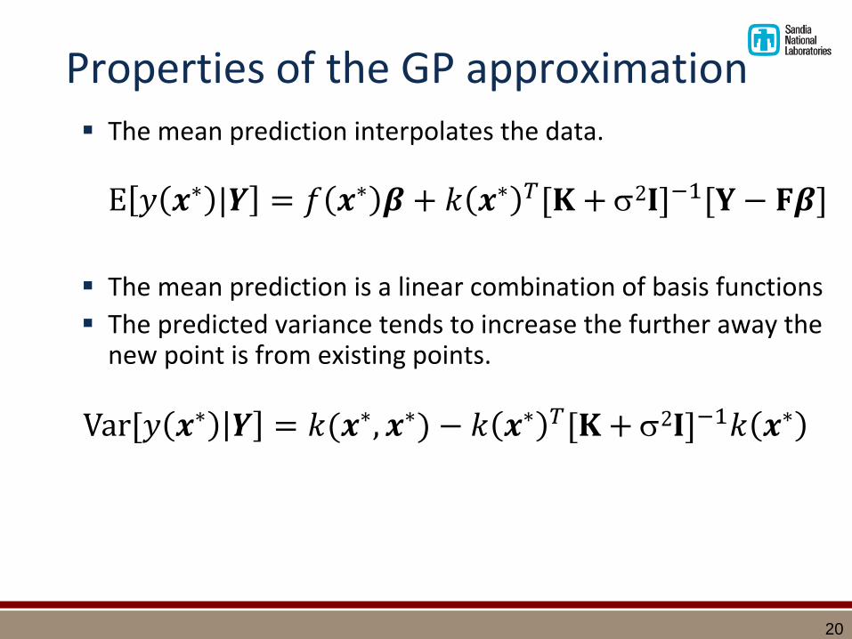
Properties of the GP approximation▪ The mean prediction interpolates the data.

E 𝑦 𝒙∗ |𝒀 = 𝑓 𝒙∗ 𝜷 + 𝑘 𝒙∗ 𝑇[𝐊 + 2𝐈]−1[𝐘 − 𝐅𝜷]

▪ The mean prediction is a linear combination of basis functions

▪ The predicted variance tends to increase the further away the new point is from existing points.

Var[𝑦 𝒙∗ 𝒀 = 𝑘(𝒙∗, 𝒙∗) − 𝑘 𝒙∗ 𝑇[𝐊 + 2𝐈]−1𝑘 𝒙∗

20

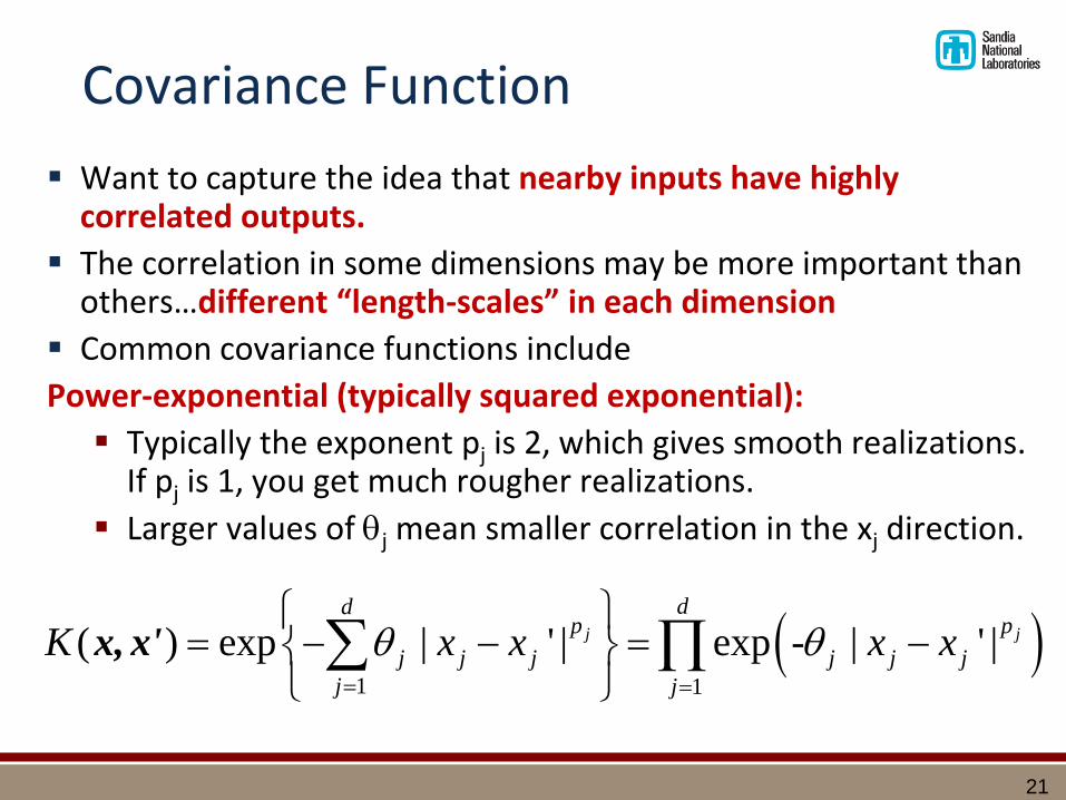
Covariance Function

▪ Want to capture the idea that nearby inputs have highly correlated outputs.

▪ The correlation in some dimensions may be more important than others…different “length-scales” in each dimension

▪ Common covariance functions include

Power-exponential (typically squared exponential):

▪ Typically the exponent pj is 2, which gives smooth realizations. If pj is 1, you get much rougher realizations.

▪ Larger values of j mean smaller correlation in the xj direction.

1 1

( ) exp | ' | exp - | ' |j j

ddp p

j j j j j j

j j

K x x x x

x, x'

21

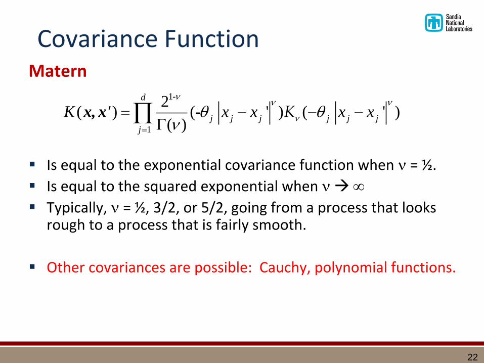
Covariance FunctionMatern

▪ Is equal to the exponential covariance function when = ½.

▪ Is equal to the squared exponential when

▪ Typically, = ½, 3/2, or 5/2, going from a process that looks rough to a process that is fairly smooth.

▪ Other covariances are possible: Cauchy, polynomial functions.

1-

1

2( ) (- ' ) ( ' )

( )

d

j j j j j j

j

K x x x x

x, x' Κ

22

Putting it all together▪ Start with N runs of a computer code, with points {xi, yi}.

Ideally, the N points will be a well-spaced design such as Latin Hypercube.

▪ Define the mean function for the Gaussian process.

▪ Often, zero mean or constant mean is used.

▪ Define the covariance function for the Gaussian process.

▪ Typically, the power-exponential function is used.

▪ Estimate the parameters governing the Gaussian process, including β, , and any parameters of the covariance function K such as j.▪ Can use maximum likelihood or Bayesian methods

▪ Substitute the parameters in the prediction equations and obtain mean and variance estimates for new points x*

23

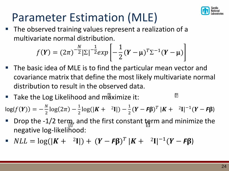
Parameter Estimation (MLE)▪ The observed training values represent a realization of a

multivariate normal distribution.

𝑓 𝒀 = (2𝜋)−𝑁2 ||−

12𝑒𝑥𝑝 −

1

2(𝒀 − )𝑇−1(𝒀 − )

▪ The basic idea of MLE is to find the particular mean vector and covariance matrix that define the most likely multivariate normal distribution to result in the observed data.

▪ Take the Log Likelihood and maximize it:

log(𝑓 𝒀) = −𝑁

2log 2𝜋 −

1

2log(|𝑲 + 2𝐈|) −

1

2(𝒀 − F𝛃)𝑇 |𝑲 + 2𝐈|−1(𝒀 − F𝛃)

▪ Drop the -1/2 term, and the first constant term and minimize the negative log-likelihood:

▪ 𝑁𝐿𝐿 = log(|𝑲 + 2𝐈|) + (𝒀 − F𝛃)𝑇 |𝑲 + 2𝐈|−1(𝒀 − F𝛃)

24

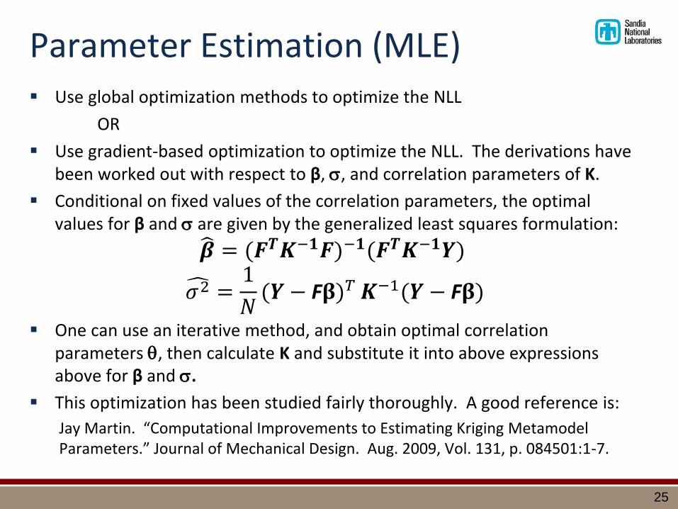
Parameter Estimation (MLE)▪ Use global optimization methods to optimize the NLL

OR

▪ Use gradient-based optimization to optimize the NLL. The derivations have been worked out with respect to β, , and correlation parameters of K.

▪ Conditional on fixed values of the correlation parameters, the optimal values for β and are given by the generalized least squares formulation:

𝜷 = (𝑭𝑻𝑲−𝟏𝑭)−𝟏(𝑭𝑻𝑲−𝟏𝒀)

𝜎2 =1

𝑁(𝒀 − F𝛃)𝑇 𝑲−1(𝒀 − F𝛃)

▪ One can use an iterative method, and obtain optimal correlation parameters , then calculate K and substitute it into above expressions above for β and .

▪ This optimization has been studied fairly thoroughly. A good reference is:

Jay Martin. “Computational Improvements to Estimating Kriging MetamodelParameters.” Journal of Mechanical Design. Aug. 2009, Vol. 131, p. 084501:1-7.

25

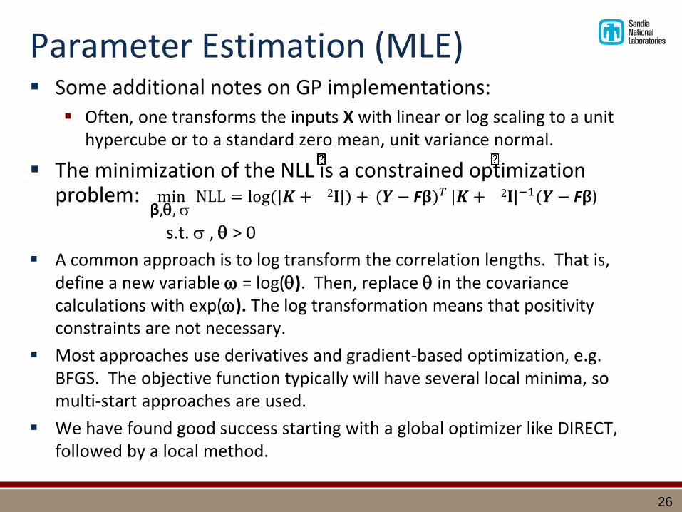
Parameter Estimation (MLE)▪ Some additional notes on GP implementations:

▪ Often, one transforms the inputs X with linear or log scaling to a unit hypercube or to a standard zero mean, unit variance normal.

▪ The minimization of the NLL is a constrained optimization problem: min

β,, NLL = log(|𝑲 + 2𝐈|) + (𝒀 − F𝛃)𝑇 |𝑲 + 2𝐈|−1(𝒀 − F𝛃)

s.t. , > 0

▪ A common approach is to log transform the correlation lengths. That is, define a new variable = log(). Then, replace in the covariance calculations with exp(). The log transformation means that positivity constraints are not necessary.

▪ Most approaches use derivatives and gradient-based optimization, e.g. BFGS. The objective function typically will have several local minima, so multi-start approaches are used.

▪ We have found good success starting with a global optimizer like DIRECT, followed by a local method.

26

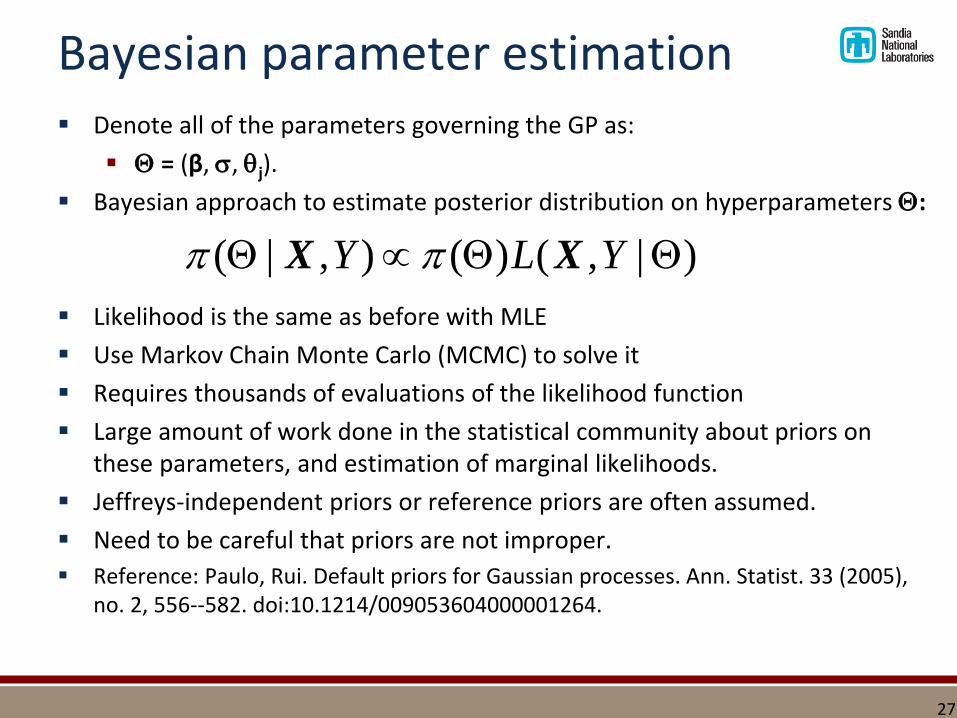
Bayesian parameter estimation▪ Denote all of the parameters governing the GP as:

▪ = (β, , j).

▪ Bayesian approach to estimate posterior distribution on hyperparameters :

▪ Likelihood is the same as before with MLE

▪ Use Markov Chain Monte Carlo (MCMC) to solve it

▪ Requires thousands of evaluations of the likelihood function

▪ Large amount of work done in the statistical community about priors on these parameters, and estimation of marginal likelihoods.

▪ Jeffreys-independent priors or reference priors are often assumed.

▪ Need to be careful that priors are not improper.

▪ Reference: Paulo, Rui. Default priors for Gaussian processes. Ann. Statist. 33 (2005), no. 2, 556--582. doi:10.1214/009053604000001264.

27

( | , ) ( ) ( , | )Y L Y X X

Experimental Design

▪ The training set of {xi} points, i= 1…N is usually a space-filling design such as a Latin Hypercube design or a maxi-min LHS

▪ Want the points to be well spaced

▪ Don’t want highly collinear points (close together)

▪ PROBLEM:

▪ The prediction calculations require the inversion of the correlation matrix

▪ Often the correlation matrix is ill-conditioned and may be numerically singular

▪ Happens even with a few hundred points in 2-D

▪ One can’t invert K to use in the prediction calculation

28

Techniques to handle ill-conditioningof the correlation matrix

▪ Remove points in a random or structured way (“Sparsification”)

▪ Often, a small “jitter” or noise term σ𝜖 is added to the diagonal terms of the covariance matrix to make the matrix better conditioned.

𝐾 → 𝐾 + σ𝜖2𝐼,

▪ Adding a nugget term ▪ Estimate the nugget as part of the measurement error

▪ Fix the measurement error and add a nugget, may have to do this iteratively until the nugget is big enough to make K well-conditioned

29

Interpretation of Gaussian Processes

30

GPs related to regression: weight-space

▪ Typical regression:

▪ In simple linear regression, we have

▪ Bayesian formalism: put a prior on the weights

▪ Can also obtain

▪ If we extend the linear regression to a more general set of basis functions , it turns out that the covariance function of a GP is

▪ Define . Then . This is called the kernel trick.

▪ Rasmussen and Williams call this framing of GPs the weight space view, see Chapter 2 of their book.

( )i iy f i

x 2~ (0, )i N T

i i iy x w

~ (0, )dN w

( | ) ( | , ) ( )p p p d y X y X w w w

( | )p w X, y

( ) x

( , ') ( ) ( )T

dk x x x x'1

2( ( )d x) x ( , ') ( ) ( )Tk x x x x'

31

GPs related to random functions

▪ A Gaussian process is a generalization of the Gaussian probability distribution. ▪ A probability distribution describes random variables

▪ A stochastic process describes the properties of functions

▪ Loosely think of a function as a long vector f(x)

▪ From our set of samples, we have a function that is a set of points {x, y(x)} or {x, f(x)}. Instead of f(x), if we use the outcome of a random draw from some joint distribution of random variables {Z(x1), … Z(xn)}, we get a realization of a random function.

▪ This is a stochastic process (e.g. generate many draws and get many functions). Constrain the functions with the data.

32

Function space view

▪ GP models place prior distributions over function spaces, and prior assumptions (e.g. smoothness, stationarity, sparsity) are encoded in covariance function

▪ Consider the Gaussian process as defining a distribution over functions, and inference taking place directly in the space of functions.

▪ Relating the two views: the squared exponential covariance function corresponds to a Bayesian linear regression model with an infinite number of basis functions.

33

GP prior and likelihood

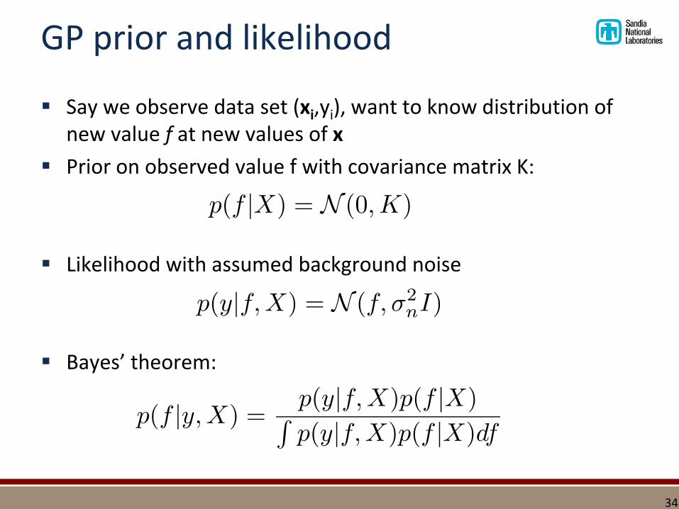
▪ Say we observe data set (xi,yi), want to know distribution of new value f at new values of x

▪ Prior on observed value f with covariance matrix K:

▪ Likelihood with assumed background noise

▪ Bayes’ theorem:

34

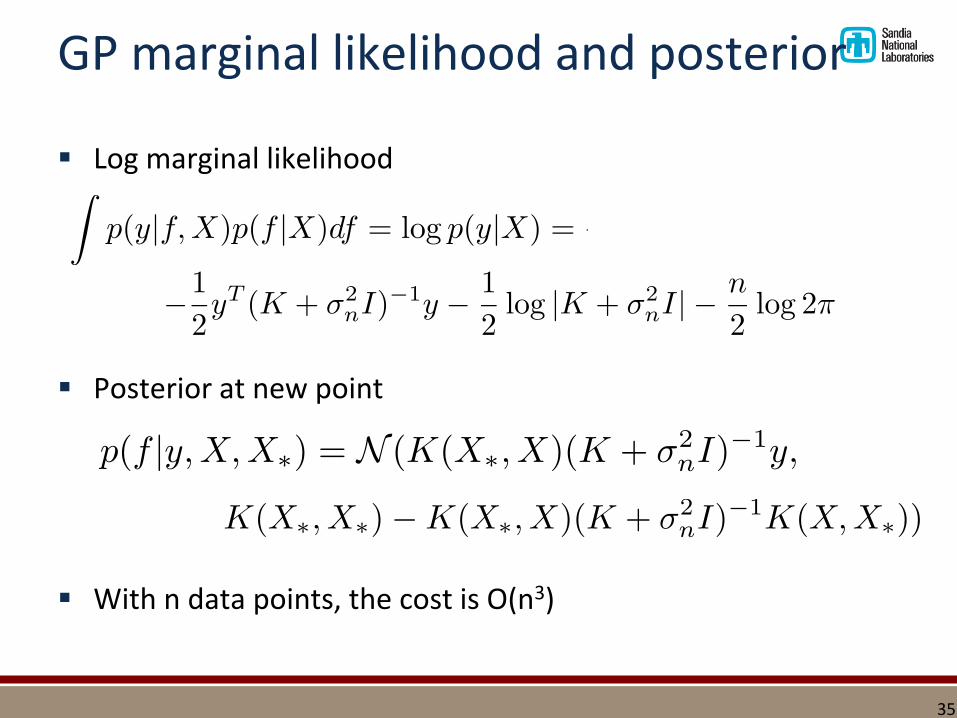
GP marginal likelihood and posterior

▪ Log marginal likelihood

▪ Posterior at new point

▪ With n data points, the cost is O(n3)

35

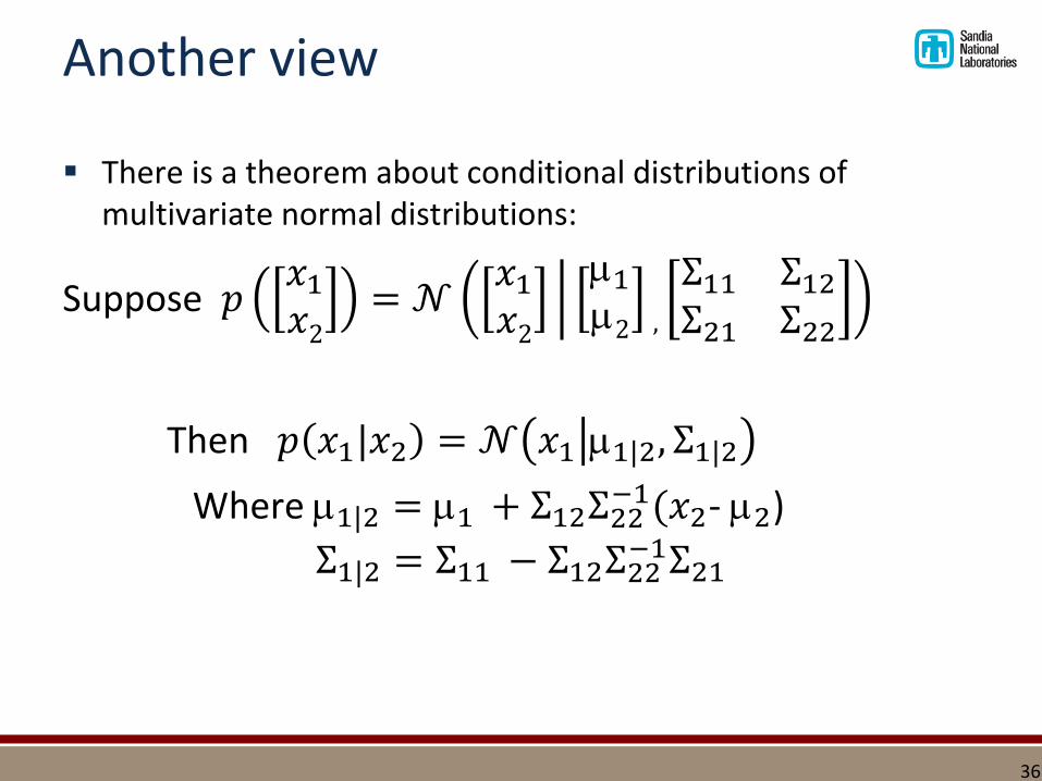
Another view

▪ There is a theorem about conditional distributions of multivariate normal distributions:

Suppose 𝑝𝑥1

𝑥2= 𝒩

𝑥1

𝑥2

1

2 ,

Σ11 Σ12

Σ21 Σ22

Then 𝑝 𝑥1|𝑥2 = 𝒩 𝑥1 1|2, Σ1|2

Where 1|2 = 1 + Σ12Σ22−1(𝑥2- 2)

Σ1|2 = Σ11 − Σ12Σ22−1Σ21

36

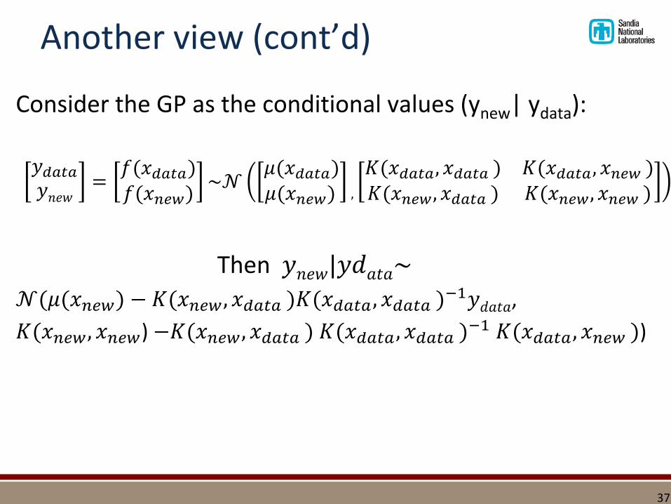
Another view (cont’d)

Consider the GP as the conditional values (ynew| ydata):

𝑦𝑑𝑎𝑡𝑎

𝑦𝑛𝑒𝑤=

𝑓(𝑥𝑑𝑎𝑡𝑎)𝑓(𝑥𝑛𝑒𝑤)

~𝒩𝜇(𝑥𝑑𝑎𝑡𝑎)𝜇(𝑥𝑛𝑒𝑤) ,

𝐾(𝑥𝑑𝑎𝑡𝑎, 𝑥𝑑𝑎𝑡𝑎 ) 𝐾(𝑥𝑑𝑎𝑡𝑎, 𝑥𝑛𝑒𝑤 )𝐾(𝑥𝑛𝑒𝑤, 𝑥𝑑𝑎𝑡𝑎 ) 𝐾(𝑥𝑛𝑒𝑤, 𝑥𝑛𝑒𝑤 )

Then 𝑦𝑛𝑒𝑤|𝑦𝑑𝑎𝑡𝑎~

𝒩(𝜇(𝑥𝑛𝑒𝑤) − 𝐾(𝑥𝑛𝑒𝑤 , 𝑥𝑑𝑎𝑡𝑎 )𝐾(𝑥𝑑𝑎𝑡𝑎 , 𝑥𝑑𝑎𝑡𝑎 )−1𝑦𝑑𝑎𝑡𝑎,

𝐾(𝑥𝑛𝑒𝑤, 𝑥𝑛𝑒𝑤) −𝐾(𝑥𝑛𝑒𝑤, 𝑥𝑑𝑎𝑡𝑎 ) 𝐾(𝑥𝑑𝑎𝑡𝑎 , 𝑥𝑑𝑎𝑡𝑎 )−1 𝐾(𝑥𝑑𝑎𝑡𝑎 , 𝑥𝑛𝑒𝑤 ))

37

Software and Resources

38

Resources

▪ Websites: www.gaussianprocess.org

▪ Managing Uncertainty in Computer Models (MUCM): ▪ UK project headed by Prof. Tony O’Hagan, University of Sheffield

▪ http://www.mucm.ac.uk/Pages/ReadingList.html

▪ Books: ▪ Gaussian Processes for Machine Learning, Carl Edward Rasmussen and

Chris Williams, MIT Press, 2006.

▪ Statistics for Spatial Data, Noel A. C. Cressie, Wiley, 1993.

▪ The Design and Analysis of Computer Experiments. Santner, T., B. Williams, and W. Notz. Springer, 2003.

39

Software and Resources

▪ Software: ▪ R: tgp (Gramacy and Lee), gptk (Kalaitzis, Lawrence, et al.), GPfit

MacDonald, Chipman, and Ranjan)

▪ Matlab: gpml (Rasmussen, Williams, Nickisch), GPmat (Sheffield Group)

▪ Python: scikit-learn. http://scikit-learn.org/stable/

▪ Python: GPy, gptools, pyGPs, etc.

▪ C++: https://github.com/mblum/libgp

▪ UQLab: https://www.uqlab.com/

▪ MIT Group: MUQ/GPEXP (Python)

▪ Dakota/Surfpack (C++), UQTk

▪ Lots of others….

40

Example: Jupyter Notebook

41

Example Use Cases

42

Where/how are Gaussian processes used?

▪ “Plain surrogate” mode: create the GP, sample it extensively to:

▪ Generate a response surface that can be plotted

▪ Perform UQ or sensitivity analysis

▪ Find the optimum of the GP

43

Example: Sampling on a Surrogate

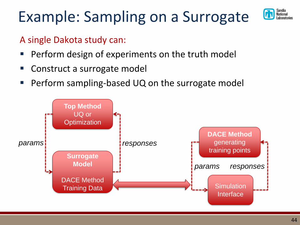
A single Dakota study can:

▪ Perform design of experiments on the truth model

▪ Construct a surrogate model

▪ Perform sampling-based UQ on the surrogate model

44

Top Method

UQ or

Optimization

DACE Method

generating

training points

Simulation

Interface

Surrogate

Model

DACE Method

Training Data

params responses

params responses

Where/how are Gaussian processes used?

▪ Adaptive mode: one advantage of the GP is its ability to generate uncertainty estimates on its predictions. There are a variety of methods that use this feature.

▪ Adaptive GPs in optimization

▪ General adaptive methods: Trust region surrogate-based optimization with data fit surrogate. Iteratively builds/validates the surrogate in each trust region

▪ Efficient Global Optimization (EGO)

▪ Adaptive GPs in reliability analysis or importance sampling

▪ Efficient global reliability analysis (EGRA), EGO interval estimation, EGO evidence theory, importance sampling (GPAIS)

45

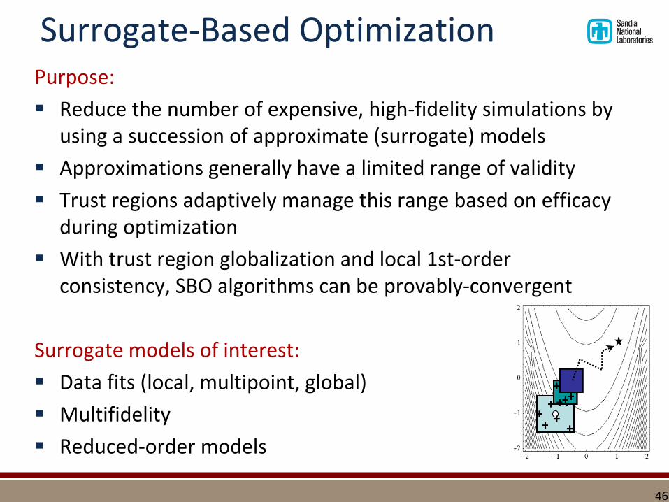
Surrogate-Based OptimizationPurpose:

▪ Reduce the number of expensive, high-fidelity simulations by using a succession of approximate (surrogate) models

▪ Approximations generally have a limited range of validity

▪ Trust regions adaptively manage this range based on efficacy during optimization

▪ With trust region globalization and local 1st-order consistency, SBO algorithms can be provably-convergent

Surrogate models of interest:

▪ Data fits (local, multipoint, global)

▪ Multifidelity

▪ Reduced-order models

46

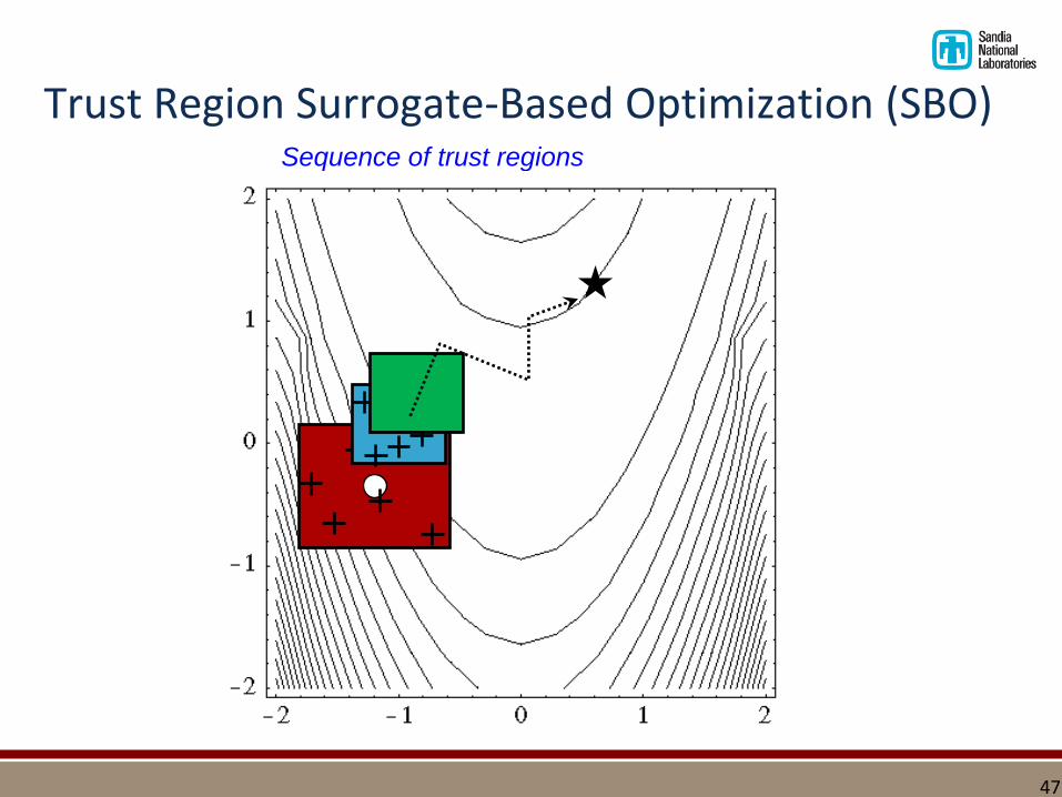
Trust Region Surrogate-Based Optimization (SBO)Sequence of trust regions

47

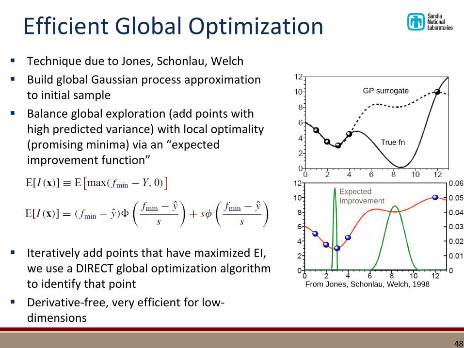
Efficient Global Optimization▪ Technique due to Jones, Schonlau, Welch

▪ Build global Gaussian process approximation to initial sample

▪ Balance global exploration (add points with high predicted variance) with local optimality (promising minima) via an “expected improvement function”

▪ Iteratively add points that have maximized EI, we use a DIRECT global optimization algorithm to identify that point

▪ Derivative-free, very efficient for low-dimensions

True fn

GP surrogate

Expected

Improvement

From Jones, Schonlau, Welch, 1998

48

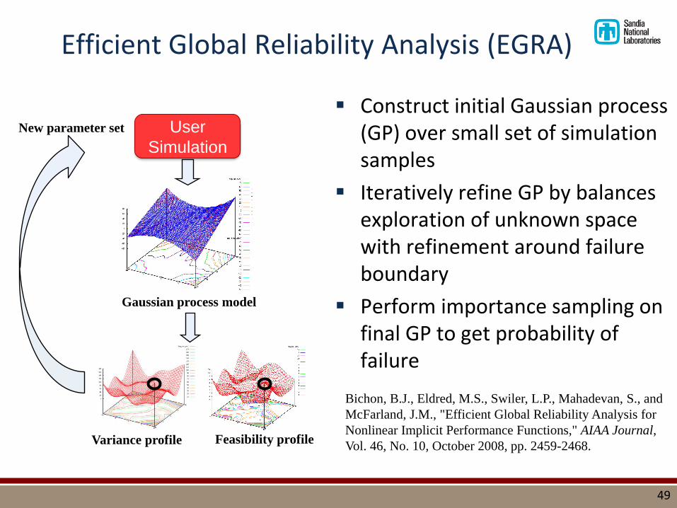
Efficient Global Reliability Analysis (EGRA)

▪ Construct initial Gaussian process (GP) over small set of simulation samples

▪ Iteratively refine GP by balances exploration of unknown space with refinement around failure boundary

▪ Perform importance sampling on final GP to get probability of failure

49

Gaussian process model

Variance profile Feasibility profile

New parameter set

Bichon, B.J., Eldred, M.S., Swiler, L.P., Mahadevan, S., and

McFarland, J.M., "Efficient Global Reliability Analysis for

Nonlinear Implicit Performance Functions," AIAA Journal,

Vol. 46, No. 10, October 2008, pp. 2459-2468.

User

Simulation

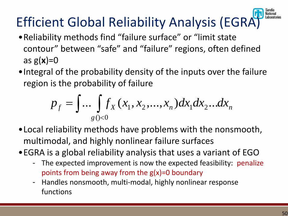
Efficient Global Reliability Analysis (EGRA)•Reliability methods find “failure surface” or “limit state

contour” between “safe” and “failure” regions, often defined as g(x)=0

•Integral of the probability density of the inputs over the failure region is the probability of failure

•Local reliability methods have problems with the nonsmooth, multimodal, and highly nonlinear failure surfaces

•EGRA is a global reliability analysis that uses a variant of EGO- The expected improvement is now the expected feasibility: penalize

points from being away from the g(x)=0 boundary- Handles nonsmooth, multi-modal, highly nonlinear response

functions

nn

g

Xf dxdxdxxxxfp ...),...,,(... 212

0()

1

50

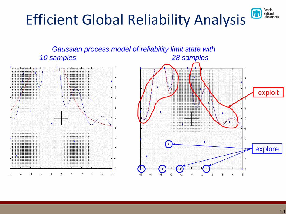
Efficient Global Reliability Analysis

Gaussian process model of reliability limit state with

10 samples 28 samples

explore

exploit

51

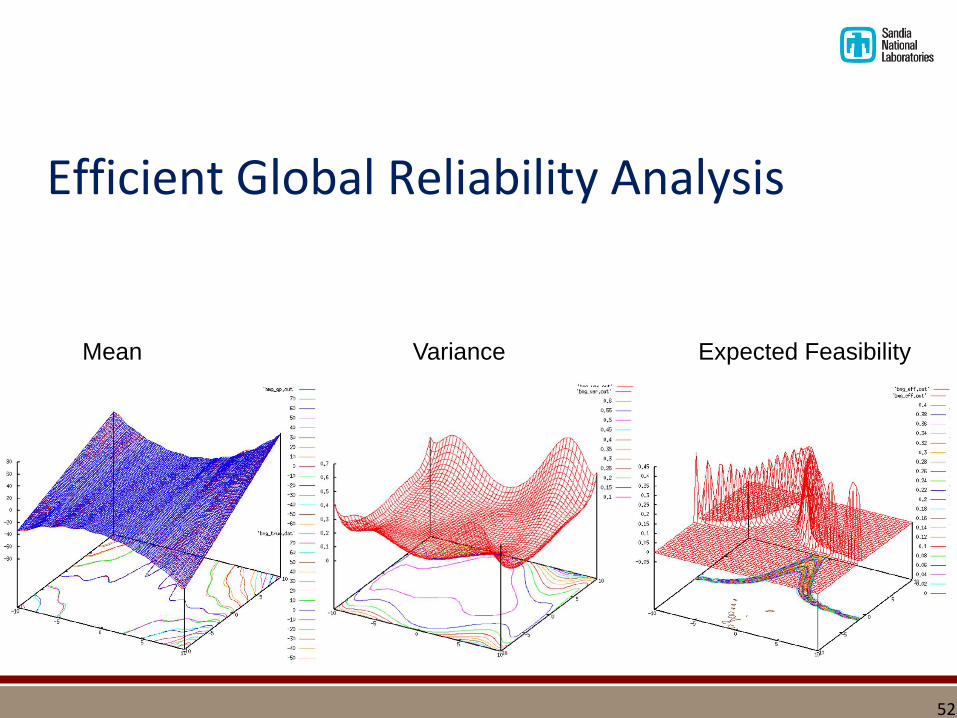
Efficient Global Reliability Analysis

Mean Variance Expected Feasibility

52

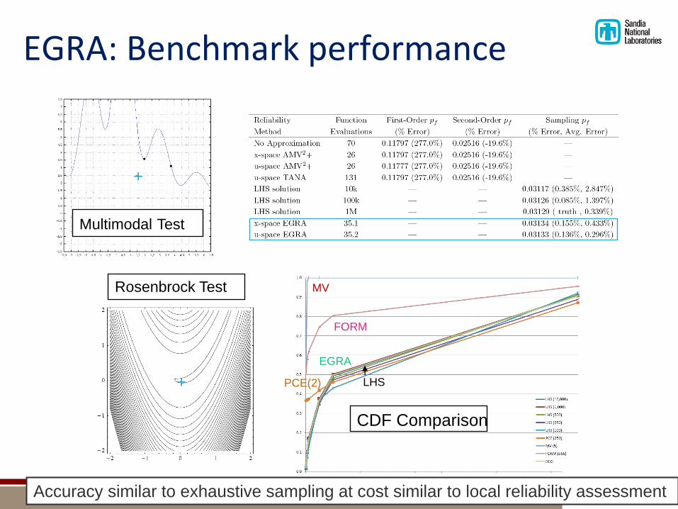
EGRA: Benchmark performance

CDF Comparison

MV

FORM

PCE(2) LHS

EGRA

Rosenbrock Test

+

Accuracy similar to exhaustive sampling at cost similar to local reliability assessment

Multimodal Test

+

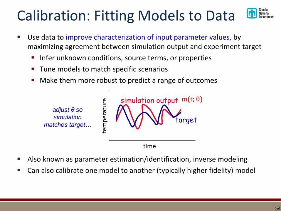
Calibration: Fitting Models to Data▪ Use data to improve characterization of input parameter values, by

maximizing agreement between simulation output and experiment target

▪ Infer unknown conditions, source terms, or properties

▪ Tune models to match specific scenarios

▪ Make them more robust to predict a range of outcomes

▪ Also known as parameter estimation/identification, inverse modeling

▪ Can also calibrate one model to another (typically higher fidelity) model

time

temperature simulation output

target

m(t; θ)

adjust θ so

simulation

matches target…

54

GP Use in Bayesian Inference

▪ Parameter calibration is a common activity in computational modeling

▪ Often, Bayesian methods are used to calibrate model parameters

▪ Monte Carlo Markov Chain (MCMC) methods are heavily used to generate posterior parameter distributions in a Bayesian framework

▪ MCMC methods require hundreds of thousands of function evaluations to converge: need to use surrogates

▪ GPs can be used within this framework

55

GP Use in Bayesian Inference

▪ NOTE: this is different from our previous discussion about viewing GPs in a Bayesian context, where the GP places a prior distribution over function spaces, and constraining the GP with “build data” is the inference process

▪ Can have a Bayesian view of GPs AND use a Bayesian framework to estimate the hyperparameters (e.g. correlation lengths, process variance) of the GP

▪ Can also use a GP within a Bayesian framework for calibration of physics model parameters

56

Bayesian Formulation

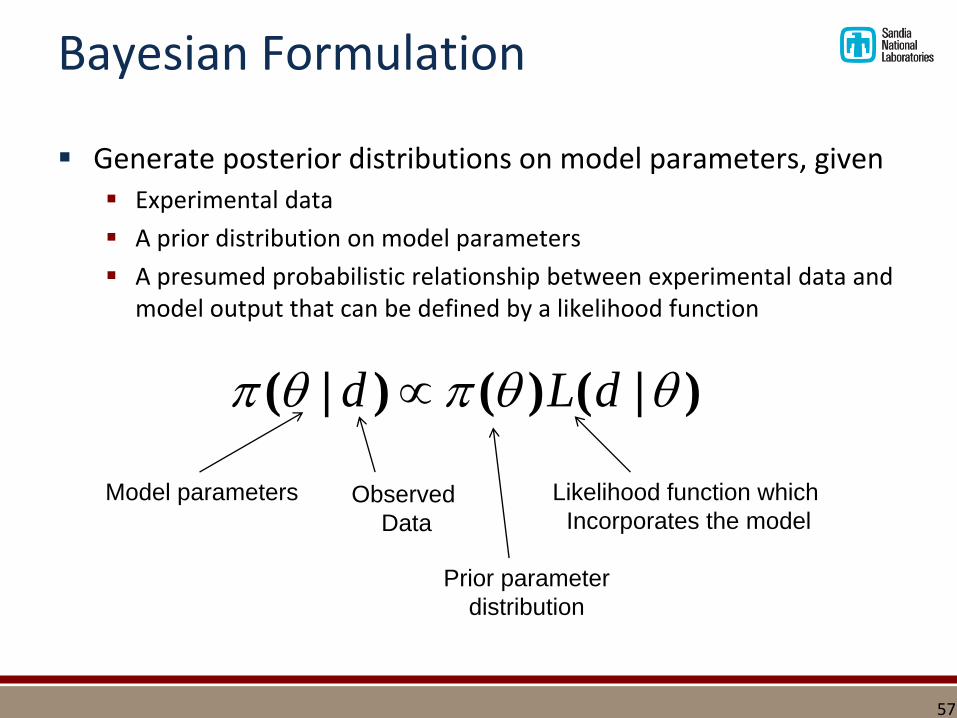
▪ Generate posterior distributions on model parameters, given▪ Experimental data

▪ A prior distribution on model parameters

▪ A presumed probabilistic relationship between experimental data and model output that can be defined by a likelihood function

57

)|()()|( dLd

Model parameters Observed

Data

Likelihood function which

Incorporates the model

Prior parameter

distribution

Bayesian Calibration of Computer Models

58

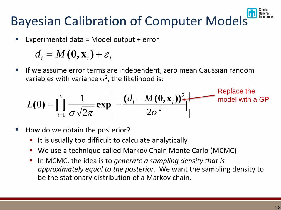
▪ Experimental data = Model output + error

▪ If we assume error terms are independent, zero mean Gaussian random variables with variance 2, the likelihood is:

▪ How do we obtain the posterior?

▪ It is usually too difficult to calculate analytically

▪ We use a technique called Markov Chain Monte Carlo (MCMC)

▪ In MCMC, the idea is to generate a sampling density that is approximately equal to the posterior. We want the sampling density to be the stationary distribution of a Markov chain.

iii Md )x,θ(

2

2

1 22

1

))x,θ((exp)θ( ii

n

i

MdL

Replace the

model with a GP

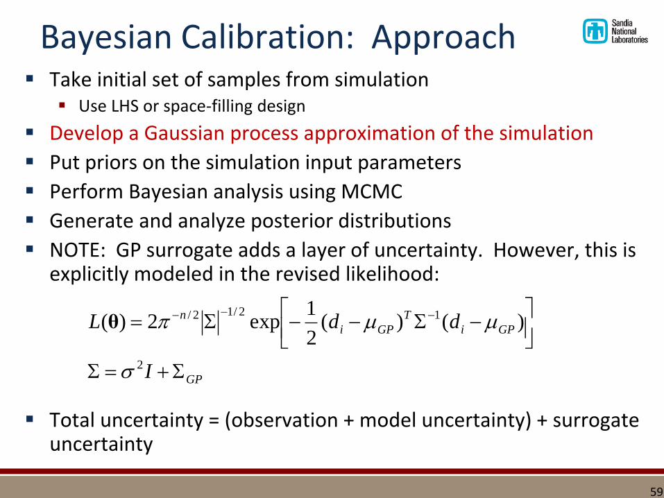
Bayesian Calibration: Approach▪ Take initial set of samples from simulation

▪ Use LHS or space-filling design

▪ Develop a Gaussian process approximation of the simulation

▪ Put priors on the simulation input parameters

▪ Perform Bayesian analysis using MCMC

▪ Generate and analyze posterior distributions

▪ NOTE: GP surrogate adds a layer of uncertainty. However, this is explicitly modeled in the revised likelihood:

▪ Total uncertainty = (observation + model uncertainty) + surrogate uncertainty

GP

GPi

T

GPi

n

I

ddL

2

12/12/ )()(2

1exp2)(

θ

59

Special Topics

▪ Constrained Gaussian Processes

▪ “Physics informed” machine learning

▪ Use of non-Gaussian likelihoods

▪ Efficient computational methods for constructing GPs, especially with large data sets

▪ Low-rank approximation

▪ Hierarchical decomposition

60

Constrained Gaussian Processes

▪ Constraints may include positivity or bound constraints on the GP model itself and/or its derivatives, linear or inequality constraints, conservation laws, rotational symmetries or invariances.

▪ How does a Gaussian process model honor physical constraints? ▪ The use of a truncated multivariate Gaussian on the output

▪ The use of non-Gaussian likelihoods which enforce the constraints

▪ The modification of the covariance function to satisfy physical constraints by a linear operator based on the physics

61

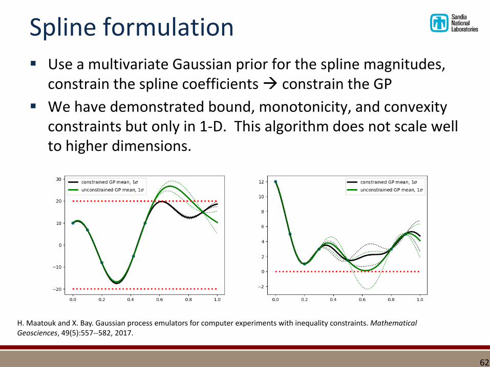
Spline formulation▪ Use a multivariate Gaussian prior for the spline magnitudes,

constrain the spline coefficients constrain the GP

▪ We have demonstrated bound, monotonicity, and convexity constraints but only in 1-D. This algorithm does not scale well to higher dimensions.

62

H. Maatouk and X. Bay. Gaussian process emulators for computer experiments with inequality constraints. Mathematical Geosciences, 49(5):557--582, 2017.

Constrained Likelihood formulation

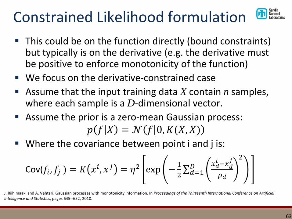
▪ This could be on the function directly (bound constraints) but typically is on the derivative (e.g. the derivative must be positive to enforce monotonicity of the function)

▪ We focus on the derivative-constrained case

▪ Assume that the input training data X contain n samples, where each sample is a D-dimensional vector.

▪ Assume the prior is a zero-mean Gaussian process: 𝑝 𝑓 𝑋 = 𝒩 𝑓 0, 𝐾(𝑋, 𝑋)

▪ Where the covariance between point i and j is:

Cov(𝑓𝑖 , 𝑓𝑗 ) = 𝐾 𝑥𝑖 , 𝑥𝑗 = 𝜂2 exp −1

2σ𝑑=1

𝐷 𝑥𝑑𝑖 −𝑥𝑑

𝑗

𝜌𝑑

2

J. Riihimaaki and A. Vehtari. Gaussian processes with monotonicity information. In Proceedings of the Thirteenth International Conference on Artificial Intelligence and Statistics, pages 645--652, 2010.

63

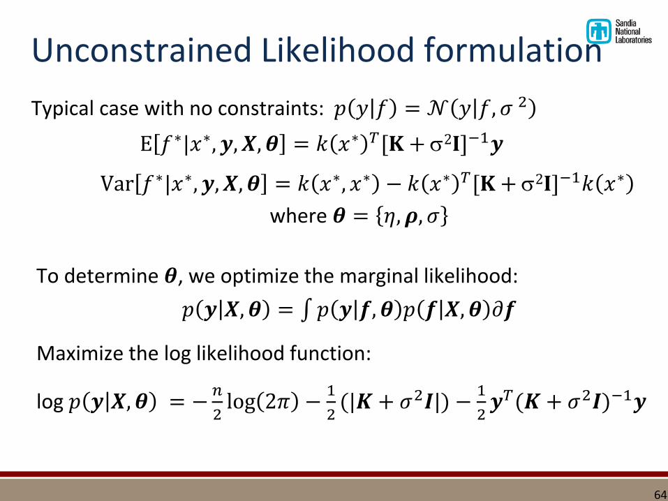
Unconstrained Likelihood formulation

Typical case with no constraints: 𝑝 𝑦 𝑓 = 𝒩 𝑦 𝑓, 𝜎 2

E 𝑓∗|𝑥∗, 𝒚, 𝑿, 𝜽 = 𝑘 𝑥∗ 𝑇[𝐊 + 2𝐈]−1𝒚

Var 𝑓∗|𝑥∗, 𝒚, 𝑿, 𝜽 = 𝑘 𝑥∗, 𝑥∗ − 𝑘 𝑥∗ 𝑇[𝐊 + 2𝐈]−1𝑘 𝑥∗

where 𝜽 = 𝜂, 𝝆, 𝜎

To determine 𝜽, we optimize the marginal likelihood:

𝑝 𝒚 𝑿, 𝜽 = 𝑝 𝒚 𝒇, 𝜽 𝑝 𝒇 𝑿, 𝜽 𝜕𝒇

Maximize the log likelihood function:

log 𝑝 𝒚 𝑿, 𝜽 = −𝑛

2log 2𝜋 −

1

2(|𝑲 + 𝜎2𝑰|) −

1

2𝒚𝑇(𝑲 + 𝜎2𝑰)−1𝒚

64

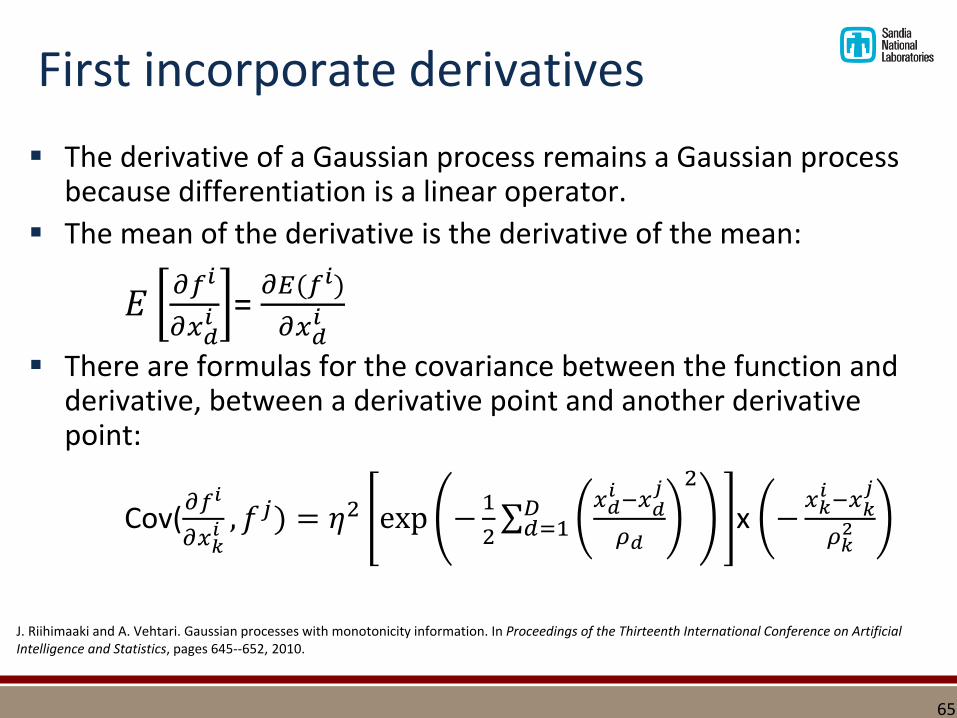
First incorporate derivatives

▪ The derivative of a Gaussian process remains a Gaussian process because differentiation is a linear operator.

▪ The mean of the derivative is the derivative of the mean:

𝐸𝜕𝑓𝑖

𝜕𝑥𝑑𝑖 =

𝜕𝐸(𝑓𝑖)

𝜕𝑥𝑑𝑖

▪ There are formulas for the covariance between the function and derivative, between a derivative point and another derivative point:

Cov(𝜕𝑓𝑖

𝜕𝑥𝑘𝑖 , 𝑓𝑗) = 𝜂2 exp −

1

2σ𝑑=1

𝐷 𝑥𝑑𝑖 −𝑥𝑑

𝑗

𝜌𝑑

2

x −𝑥𝑘

𝑖 −𝑥𝑘𝑗

𝜌𝑘2

J. Riihimaaki and A. Vehtari. Gaussian processes with monotonicity information. In Proceedings of the Thirteenth International Conference on Artificial Intelligence and Statistics, pages 645--652, 2010.

65

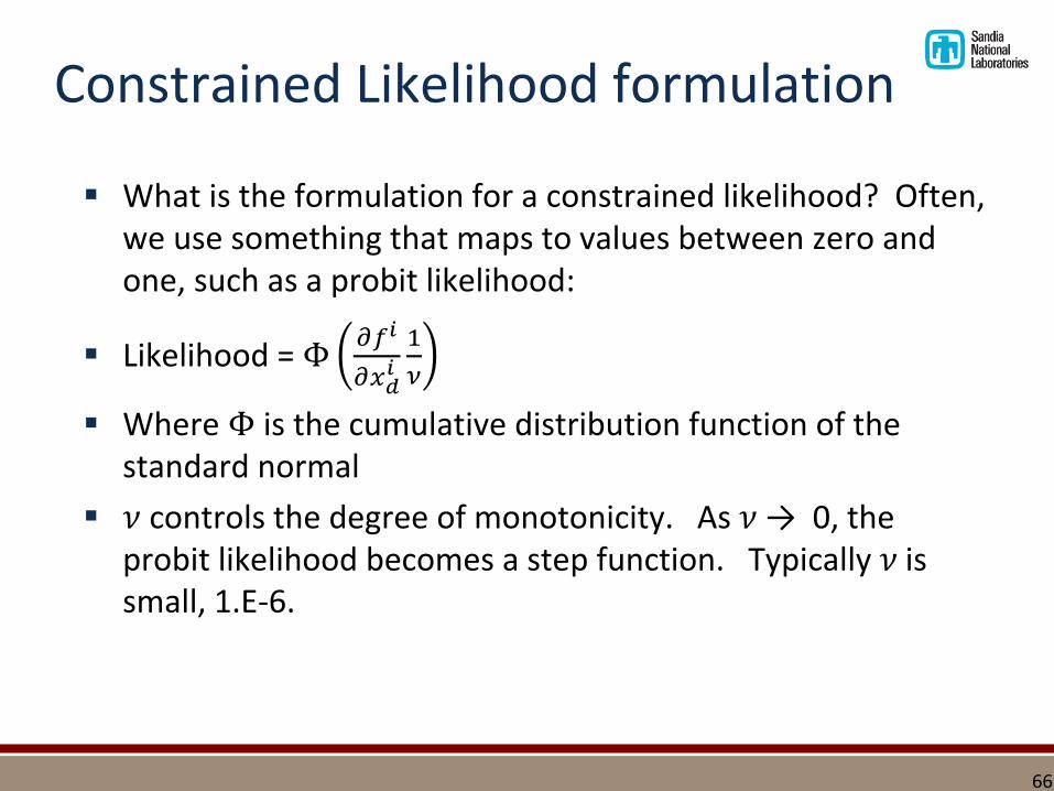
Constrained Likelihood formulation

▪ What is the formulation for a constrained likelihood? Often, we use something that maps to values between zero and one, such as a probit likelihood:

▪ Likelihood = Φ𝜕𝑓𝑖

𝜕𝑥𝑑𝑖

1

𝜈

▪ Where Φ is the cumulative distribution function of the standard normal

▪ 𝜈 controls the degree of monotonicity. As 𝜈 → 0, the probit likelihood becomes a step function. Typically 𝜈 is small, 1.E-6.

66

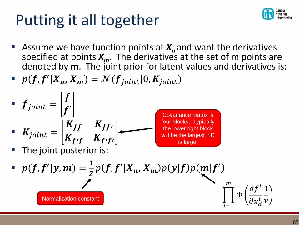
Putting it all together

▪ Assume we have function points at Xn and want the derivatives specified at points Xm. The derivatives at the set of m points are denoted by m. The joint prior for latent values and derivatives is:

▪ 𝑝(𝒇, 𝒇′|𝑿𝒏, 𝑿𝒎) = 𝒩(𝒇𝑗𝑜𝑖𝑛𝑡|0, 𝑲𝑗𝑜𝑖𝑛𝑡)

▪ 𝒇𝑗𝑜𝑖𝑛𝑡 =𝒇

𝒇′

▪ 𝑲𝑗𝑜𝑖𝑛𝑡 =𝑲𝒇𝒇 𝑲𝒇𝒇′

𝑲𝒇′𝒇 𝑲𝒇′𝒇′

▪ The joint posterior is:

▪ 𝑝(𝒇, 𝒇′|𝒚, 𝒎) =1

𝑍𝑝 𝒇, 𝒇′ 𝑿𝒏, 𝑿𝒎 𝑝 𝒚 𝒇 𝑝 𝒎 𝒇′

Covariance matrix is

four blocks. Typically

the lower right block

will be the largest if D

is large.

Normalization constantෑ

𝑖=1

𝑚

Φ𝜕𝑓𝑖

𝜕𝑥𝑑𝑖

1

𝜈

67

Putting it all together

▪ How do we work with the joint posterior and determine its hyperparameters?

▪ We used MCMC. One could also use Laplace approximation to the posterior or expectation propagation.

▪ Appended 𝜽 = 𝜂, 𝝆, 𝜎 to the vector over which the MCMC was operating to be: 𝒇, 𝒇′, 𝜂, 𝝆, 𝜎

68

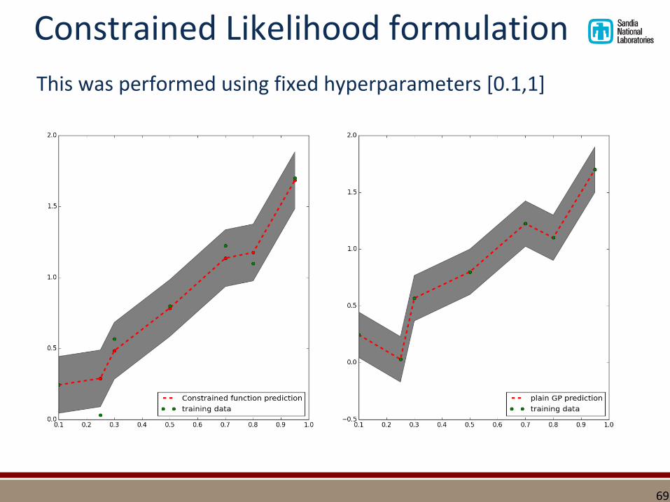
This was performed using fixed hyperparameters [0.1,1]

Constrained Likelihood formulation

69

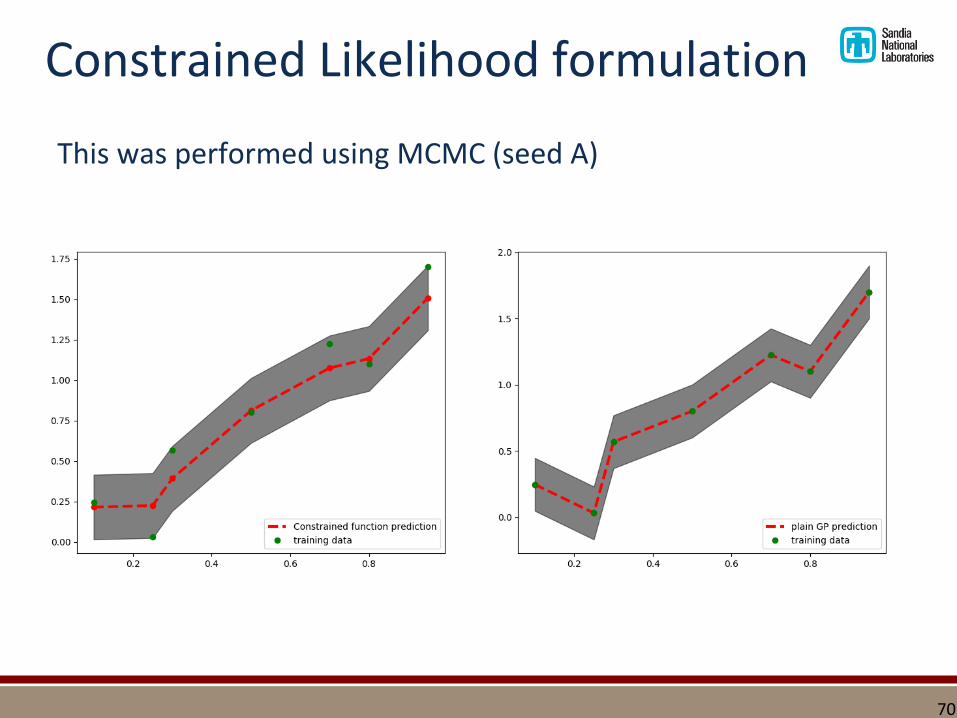
This was performed using MCMC (seed A)

Constrained Likelihood formulation

70

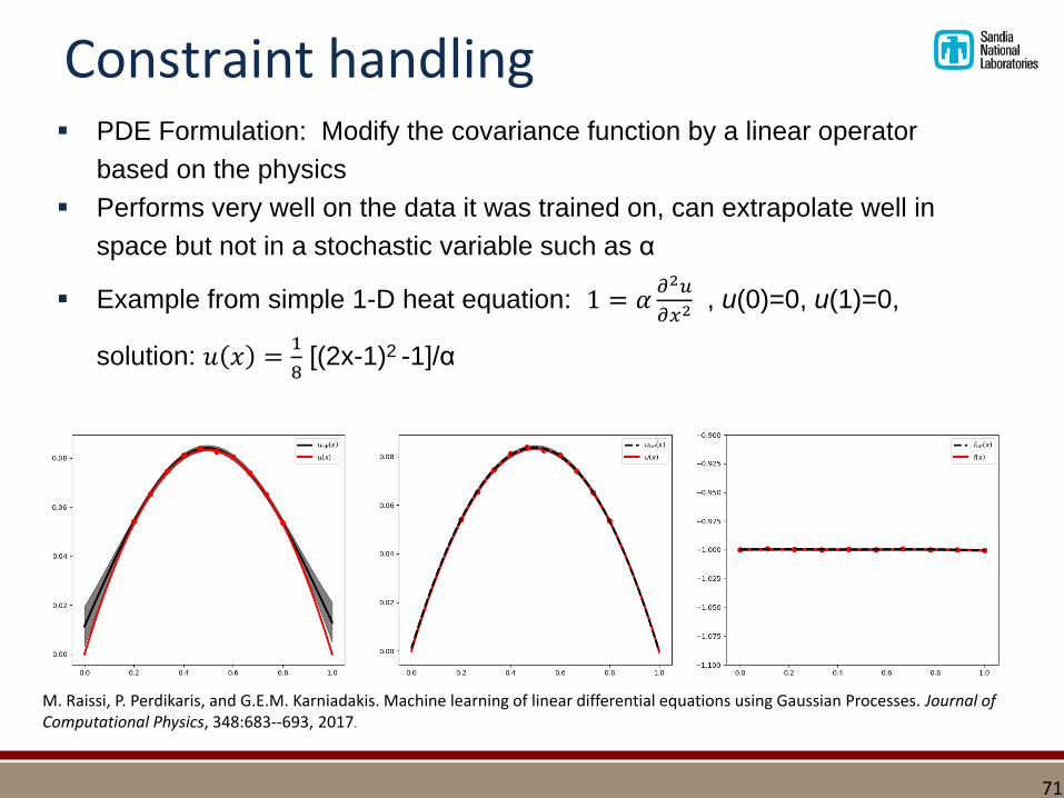
Constraint handling▪ PDE Formulation: Modify the covariance function by a linear operator

based on the physics

▪ Performs very well on the data it was trained on, can extrapolate well in

space but not in a stochastic variable such as α

▪ Example from simple 1-D heat equation: 1 = 𝛼𝜕2𝑢

𝜕𝑥2 , u(0)=0, u(1)=0,

solution: 𝑢 𝑥 =1

8[(2x-1)2 -1]/α

71

M. Raissi, P. Perdikaris, and G.E.M. Karniadakis. Machine learning of linear differential equations using Gaussian Processes. Journal of Computational Physics, 348:683--693, 2017.

Computational Efficiencies for GPs

72

GP Performance▪ How do we expect inference to change as we add more data, more

dimensions, more complexity/non-stationarity in the underlying function?

▪ More data typically improves the inference, reduces the GP predictive variance, and results in better estimation of the covariance function parameters. BUT this comes at a computational cost.

▪ You can add a more expressive kernel, but it requires more data to train, which makes it more expensive.

▪ If the kernel is exactly specified, there is fast convergence in error. But we never actually have the right kernel.

▪ A "vanilla" GP implementation is limited to about 10,000 data points without employing some of approaches we will discuss.

▪ This is not just due to ill-conditioning of the covariance matrix.

▪ The covariance matrix is an N2 dense matrix and inversion/Cholesky has a cost of N3. Most computers can’t handle a problem that size.

73

Techniques to handle ill-conditioningof the correlation matrix

▪ Remove points in a random or structured way (“Sparsification”)

▪ Often, a small “jitter” or noise term σ𝜖 is added to the diagonal terms of the covariance matrix to make the matrix better conditioned.

𝐾 → 𝐾 + σ𝜖2𝐼,

▪ Adding a nugget term ▪ Estimate the nugget as part of the measurement error

▪ Fix the measurement error and add a nugget, may have to do this iteratively until the nugget is big enough to make K well-conditioned

74

Techniques to handle ill-conditioningof the correlation matrix (cont’d)

▪ Linear algebra tricks▪ Don’t take the inverse of K, take the Cholesky factorization

▪ Pseudo-inverse

▪ Discards small singular values

▪ Pivoted Cholesky Factorization

▪ discard additional copies of the information that is most duplicated

▪ Decrease the maximum eigenvalue and increase the minimum eigenvalue

▪ Gradient-enhanced kriging

▪ SAND Report 2013-7022. Efficient and Robust Gradient Enhanced Kriging Emulators, by Keith Dalbey.

75

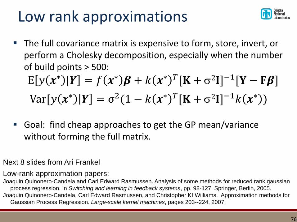
Low rank approximations

▪ The full covariance matrix is expensive to form, store, invert, or perform a Cholesky decomposition, especially when the number of build points > 500:

E 𝑦 𝒙∗ |𝒀 = 𝑓 𝒙∗ 𝜷 + 𝑘 𝒙∗ 𝑇[𝐊 + 2𝐈]−1[𝐘 − 𝐅𝜷]

Var[𝑦 𝒙∗ 𝒀 = σ2(1 − 𝑘 𝒙∗ 𝑇[𝐊 + 2𝐈]−1𝑘 𝒙∗ )

▪ Goal: find cheap approaches to get the GP mean/variance without forming the full matrix.

Next 8 slides from Ari Frankel

Low-rank approximation papers:Joaquin Quinonero-Candela and Carl Edward Rasmussen. Analysis of some methods for reduced rank gaussian

process regression. In Switching and learning in feedback systems, pp. 98-127. Springer, Berlin, 2005.

Joaquin Quinonero-Candela, Carl Edward Rasmussen, and Christopher KI Williams. Approximation methods for

Gaussian Process Regression. Large-scale kernel machines, pages 203--224, 2007.

76

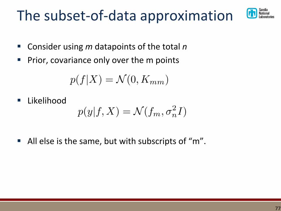
The subset-of-data approximation

▪ Consider using m datapoints of the total n

▪ Prior, covariance only over the m points

▪ Likelihood

▪ All else is the same, but with subscripts of “m”.

77

The subset-of-datapoints approximation

▪ Cost is O(m3)

▪ Pros:

▪ Cheap, especially if you can get low error with small number of points

▪ Pick points cleverly/greedily

▪ Add points with largest predictive variance (equivalent to largest differential entropy) or that would increase the KL-divergence between current posterior and new posterior

▪ Cons:

▪ Wasteful of data!

78

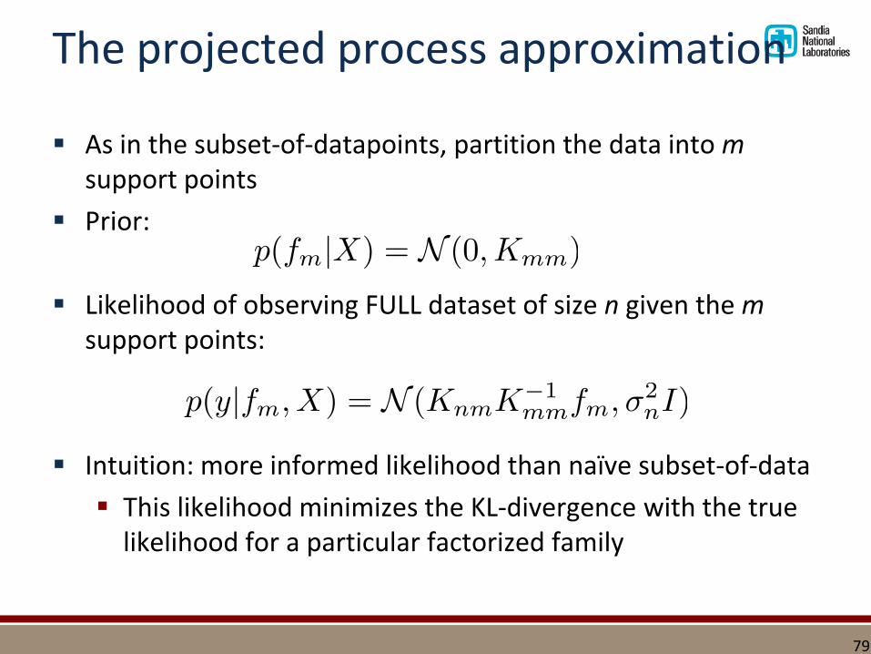
The projected process approximation

▪ As in the subset-of-datapoints, partition the data into msupport points

▪ Prior:

▪ Likelihood of observing FULL dataset of size n given the msupport points:

▪ Intuition: more informed likelihood than naïve subset-of-data

▪ This likelihood minimizes the KL-divergence with the true likelihood for a particular factorized family

79

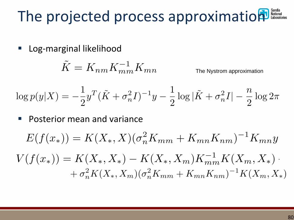
The projected process approximation

▪ Log-marginal likelihood

▪ Posterior mean and variance

The Nystrom approximation

80

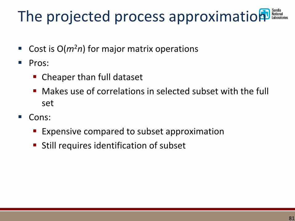
The projected process approximation

▪ Cost is O(m2n) for major matrix operations

▪ Pros:

▪ Cheaper than full dataset

▪ Makes use of correlations in selected subset with the full set

▪ Cons:

▪ Expensive compared to subset approximation

▪ Still requires identification of subset

81

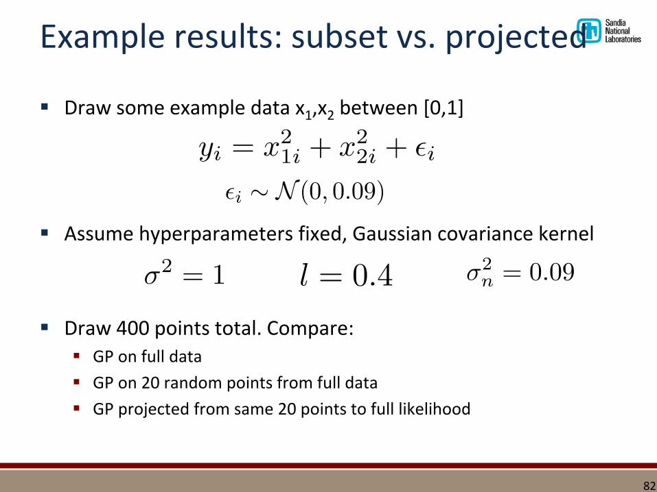
Example results: subset vs. projected

▪ Draw some example data x1,x2 between [0,1]

▪ Assume hyperparameters fixed, Gaussian covariance kernel

▪ Draw 400 points total. Compare:▪ GP on full data

▪ GP on 20 random points from full data

▪ GP projected from same 20 points to full likelihood

82

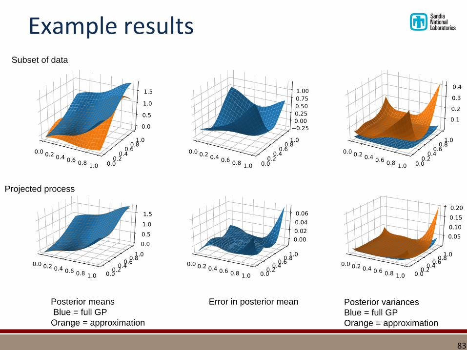
Example results

Posterior means

Blue = full GP

Orange = approximation

Error in posterior mean Posterior variances

Blue = full GP

Orange = approximation

Subset of data

Projected process

83

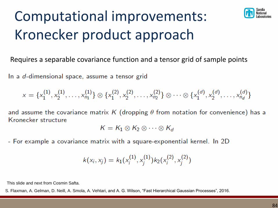
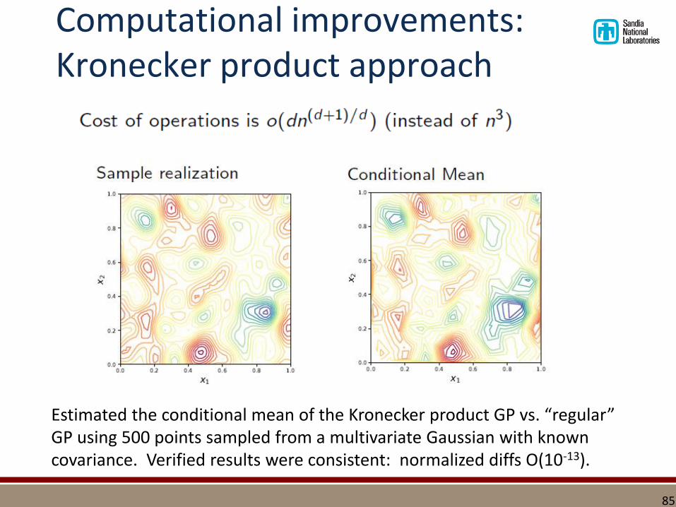
Computational improvements: Kronecker product approach

84

Requires a separable covariance function and a tensor grid of sample points

S. Flaxman, A. Gelman, D. Neill, A. Smola, A. Vehtari, and A. G. Wilson, “Fast Hierarchical Gaussian Processes”, 2016.

This slide and next from Cosmin Safta.

85

Estimated the conditional mean of the Kronecker product GP vs. “regular” GP using 500 points sampled from a multivariate Gaussian with known covariance. Verified results were consistent: normalized diffs O(10-13).

Computational improvements: Kronecker product approach

THANK YOU! QUESTIONS?

86