gasp: the genetic algorithm for structure and … the genetic algorithm for structure and phase...

GASP: The Genetic Algorithm for Structure and

Phase Prediction

Will Tipton and Richard Hennig

Last updated: April 25, 2014

Abstract

The GASP code is contains a heuristic search algorithm to solve theatomic structure prediction problems. It includes most successful

techniques described in the literature and a few important new ones. Itcan search for crystalline structures as well as those with periodicity infewer than 3 dimensions. It is interfaced with a number of energy codesincluding GULP, VASP, and LAMMPS. This document describes themethodology behind the project as well as the practical aspects of the

code’s implementation and use.

Contents

1 Methodology 31.1 Context and motivation . . . . . . . . . . . . . . . . . . . . . 31.2 The biological analogy . . . . . . . . . . . . . . . . . . . . . . 41.3 Reframing the structure prediction problem . . . . . . . . . . 41.4 Details of our approach . . . . . . . . . . . . . . . . . . . . . 5

1.4.1 Structure representation . . . . . . . . . . . . . . . . . 51.4.2 Energy, value and fitness . . . . . . . . . . . . . . . . 51.4.3 The algorithm . . . . . . . . . . . . . . . . . . . . . . 51.4.4 Selection . . . . . . . . . . . . . . . . . . . . . . . . . 61.4.5 Variations and their motivation . . . . . . . . . . . . . 71.4.6 Constraints and reducing the size of the solution space 111.4.7 Local relaxation . . . . . . . . . . . . . . . . . . . . . 121.4.8 Development . . . . . . . . . . . . . . . . . . . . . . . 121.4.9 Avoiding redundant calculations . . . . . . . . . . . . 131.4.10 Endgame . . . . . . . . . . . . . . . . . . . . . . . . . 14

2 Usage 152.1 Input . . . . . . . . . . . . . . . . . . . . . . . . . . . . . . . . 15

2.1.1 The main input file . . . . . . . . . . . . . . . . . . . . 152.2 Output . . . . . . . . . . . . . . . . . . . . . . . . . . . . . . 21

2.2.1 Output to disk . . . . . . . . . . . . . . . . . . . . . . 212.2.2 Output to screen . . . . . . . . . . . . . . . . . . . . . 212.2.3 Visualizing output . . . . . . . . . . . . . . . . . . . . 22

2.3 Energy code interfaces . . . . . . . . . . . . . . . . . . . . . . 222.3.1 Gulp . . . . . . . . . . . . . . . . . . . . . . . . . . . . 232.3.2 Vasp . . . . . . . . . . . . . . . . . . . . . . . . . . . . 242.3.3 LAMMPS . . . . . . . . . . . . . . . . . . . . . . . . . 24

2.4 Resuming calculations . . . . . . . . . . . . . . . . . . . . . . 252.5 Strategies . . . . . . . . . . . . . . . . . . . . . . . . . . . . . 26

3 Implementation 273.1 General strategy . . . . . . . . . . . . . . . . . . . . . . . . . 273.2 Randomness . . . . . . . . . . . . . . . . . . . . . . . . . . . . 27

1

3.3 The main loop . . . . . . . . . . . . . . . . . . . . . . . . . . 273.4 ObjectiveFunction and Energy . . . . . . . . . . . . . . . . . 283.5 Genetic operators . . . . . . . . . . . . . . . . . . . . . . . . . 28

3.5.1 Selection . . . . . . . . . . . . . . . . . . . . . . . . . 283.5.2 Variation . . . . . . . . . . . . . . . . . . . . . . . . . 293.5.3 Promotion . . . . . . . . . . . . . . . . . . . . . . . . . 293.5.4 Development . . . . . . . . . . . . . . . . . . . . . . . 29

3.6 Organisms . . . . . . . . . . . . . . . . . . . . . . . . . . . . . 293.6.1 Organism representation and StructureOrg . . . . . . 293.6.2 Generation and Structures . . . . . . . . . . . . . . . . 303.6.3 Initial population . . . . . . . . . . . . . . . . . . . . . 303.6.4 Fitness and value . . . . . . . . . . . . . . . . . . . . . 30

3.7 Convergence . . . . . . . . . . . . . . . . . . . . . . . . . . . . 313.8 Input and parameters . . . . . . . . . . . . . . . . . . . . . . 313.9 Parallelization . . . . . . . . . . . . . . . . . . . . . . . . . . . 313.10 Description of files . . . . . . . . . . . . . . . . . . . . . . . . 323.11 Modifying the code . . . . . . . . . . . . . . . . . . . . . . . . 36

3.11.1 Example: adding a parameter . . . . . . . . . . . . . . 363.11.2 Example: testing new variations . . . . . . . . . . . . 36

A Main loop 38

B Using GridEngine and Vasp 40

C Example input file 42

D Scripts for testing parameters 43

References 46

2

Chapter 1

Methodology

NB: Both the review of the literature and the discussion of our ownmethodology in this chapter are out of date. For a more recent literaturereview, please see [13], and for a description of our own work, please see[14]

1.1 Context and motivation

Many practical materials science problems are effectively the search for a materialwith certain properties. Determining the structure of a material is an importantfirst step in finding its properties without experimental work. There have beensuccesses in approaching the structure prediction problem through examination ofknown materials, both intuition-based and not [6]. However, there would be someadvantage to a first-principles method. Such a method would work on a large classof materials without relying on intuition and would be able to predict structurescompletely different from those already known.

The stable structure of a material will be that which minimizes its quantum-mechanical free energy. So, the structure prediction problem is equivalent to theproblem of finding the global minimium of the energy functional, which becomes ourfocus. Now, in general we have no analytical expression for the energy functional;we can only compute it for specific inputs. So we must perform some sort of guess-and-check type search over the space of solutions.

A number of search strategies have been implemented and tested includingsimulated annealing, minima hopping, and some monte-carlo methods. However,genetic algorithms modeled after natural evolution have shown much promise, andthat is what we implement here. Glass et. al. have a good discussion of why thegenetic strategy is particularly well suited to this problem.[8]

The evolutionary approach has also been tried a few times before [4] [5] [7] [9][8] [12] [15] [16] . Here, we implement and evaluate techniques described in thisliterature as well as several improvements of our own.

3

1.2 The biological analogy

In nature, genetic information is carried in organisms. It is maintained in a popu-lation’s gene pool if it is passed through reproduction to successful offspring. Newinformation can be introduced to the gene pool through mutation events, but theseare rare (and usually lethal). The success that an organism has in passing on itsgenes is often given a value between zero and one and called the organism’s fitness.

The fitness of an organism is not universal but depends on its environment.A lion would do poorly in the Arctic and a great-white shark would do poorly inKansas. More subtly, there is variance of traits within a single species. In somecases, these differences can lead to a difference in the organisms’ fitness. Thus, therelevant traits of the higher-fitness individuals are likely to be more common insubsequent generations. In this way populations (but not individuals) evolve to bewell suited to their environment.

This assumes, of course, the well understood fact that relevant traits are passedon, to varying degrees, from parents to offspring. The correlation between a traitin a parent and that in an offspring is known as the heritability of a trait. In orderfor environmental pressure to cause quick evolution in a trait, that trait must havea high heritability.

1.3 Reframing the structure prediction problem

The evolutionary approach to structure prediction is modeled after the naturalprocess. Each crystal structure is considered an organism. The representationdescribed in 1.4.1 will be its “genotype.” In nature, the fitness of an organism isbased on how well its phenotype is suited to its environment and, in particular, howsuccessful it is in reproducing. We assign fitnesses to the organisms based on theirenergies and allow them to reproduce probabilistically based on those fitnesses.Pressures analogous to those which force species to adapt to their environmentswill thus lead to lower energy crystal structures.

We organize organisms into generations. The algorithm proceeds by creatingsuccessive generations. The methods by which an offspring generation is madefrom parents are called variation operations or variations. They include operationswhich are analogous to genetic mutation and crossover. Each time the algorithmwants to create a new organism using a variation, it must select parents usinga selection method. Each offspring must meet some minimum standards to beconsidered viable, analogous to the “growing up” process in nature. We call thisthe development stage.

We also try to improve on the biological analogy when possible. In particular,we would rather not let the most optimal solution worsen from one algorithmiciteration to the next. So, we implement a promotion operation which promotessome number of the best organisms from one generation directly to the next. Also,mutations in nature are usually detrimental. We try to use mutation variationswhich are likely to introduce valuable new information to the gene pool.

4

1.4 Details of our approach

1.4.1 Structure representation

We consider primarily 3D-periodic or crystalline structures – atomic clusters, sur-faces, etc. are generally dealt with by packaging them into a large box with anappropriate amount of vacuum spacing. So, a description of one cell determinesthe whole system. In particular, we will work with the six lattice parameters andthe 3N atomic coordinates of a cell where N is the number of atoms in the cell.The lattice parameters include three angles, usually represented in degrees, andthree lengths, generally given in Angstroms. For most purposes, we will write thefractional coordinates of atoms in a cell.

In total, this gives 3N + 6 variables needed to describe solutions. Additionally,in ab-initio applications, N itself must usually be determined. However, theseare not truly independent degrees of freedom: there are infinitely many ways torepresent the same structure. In addition to differently-sized supercells, any affinetransformation of the atomic positions or alternate choice of lattice vectors mayproduce an alternate representation of a single crystal structure.

In biological language, there are many genotypes which produce each pheno-type. Since our solution space is somewhat more complicated than it has to be, ourproblem of searching that space is more complicated than it, in theory, has to be.In practice, we will try to focus our attention on one representative portion of thespace. This way, variations which act on a particular representation will have highheritabilities.

1.4.2 Energy, value and fitness

There are subtle but important relationships between the values we will call theenergy, value and fitness of an organism. The energy is the total energy as computedby some total energy code. The value of an organism is the number returned bythe objective function. For example, if we are using EnergyPerAtom then the valueof an organism will be its energy divided by the number of atoms in its cell.

An organism’s fitness is its value normalized in the context of its generation.In particular, an organism with value value has fitness given by

f =value− worstV alue

bestV alue− worstV alue

where worstV alue and bestV alue are the highest and lowest energies in the currentgeneration. So, the lowest energy organism has a fitness of 1 and the highest energyorganism has a fitness of 0.

1.4.3 The algorithm

Abstractly and without parallelization, the genetic algorithm proceeds as follows:

1. Create initial parents generation.

2. Create empty offspring generation.

3. Apply promotion and variation operations to create offspring.

(a) If we have enough offspring, go to 4.

5

(b) Apply a random variation to one or two randomly chosen organismsfrom the parent generation to create an offspring.

(c) Develop the offspring.

4. Relax each structure and evaluate its fitness.

5. Re-develop each offspring and, if successful, add it to the generation.

6. If converged, end.

7. Set offspring → parents.

8. Go to 2.

See Appendix A for a complete code listing.

1.4.4 Selection

In nature, organisms of higher fitness are by definition more likely to successfullyreproduce. In the genetic algorithm, we select those organisms to reproduce whichwe would like to be successful, that is, those with lower total energies. Preferentialselection of lower energy organisms to act as parents is the only major evolutionary“force” that is acting. If we allowed all organisms equal probability of reproduction,the population as a whole would have no incentive to improve.

There are several commonly-used selection strategies: elitist, roulette, and tour-nament. Elitist is also known as simple and just means that the top numParentsorganisms are allowed to reproduce with equal probability [9]. In roulette selection,a random number d between 0 and 1 is chosen for each organism, and if d is lessthan the fitness of the organism, it is allowed to reproduce [4]. In this way, it ispossible for any organism to reproduce (except the worst one which has fitness 0),but it is more likely for organisms of higher fitness. Finally, in tournament selection,all of the organisms in the parent generation are randomly grouped into pairs, andthe better member of each pair is allowed to reproduce. Tournament and roulettemethods have very similar results.

In order to test selection strategies, we use a method which is more or less ageneralization of the three above: organisms are selected on the basis of a normal-ized probability distribution over their fitnesses. Two parameters are specified todescribe the distribution: numParents and selectionPower. numParents is thenumber of organisms we will allow the possibility of being parents. selectionPowerdetermines the power-law which comprises the rest of the distribution. We will referto different selection strategies with an ordered pair containing these two numbers:

(numParents, selectionPower)

So, for example, in a population of size 20, (5, 0) selection is an elitist strategy, and(20, 1) selection is a roulette strategy.

In more detail, we first set to zero the selection probabilities of organisms worsethan the numParents+1th best. We then recalculate the fitnesses of the remainingorganisms with respect to the remaining “sub-generation” in the same way whichfitnesses are normally calculated, except that we are only considering a portion ofa generation. The selection probability of a remaining organism with renormalizedfitness fi is set to

pi =fni∑j f

nj

6

where n = selectionPower and the sum is over the top numParents organisms.Clearly,

∑i pi = 1, and our distribution is normalized. The renormalization was

necessary so that the probability distribution is continuous.

Figure 1.1: Example selection probability distributions of a generation with 21members with evenly-spaced fitnesses. In order of aggressiveness, we have a (5, 0)elitist distribution in red, a (15, 2) selection in green, a (14, 1) selection in blue, anda (18, 0.5) selection in cyan.

Figure 1.1 shows some examples. Elitist selection, as described above, can beachieved by choosing a small numParents and setting selectionPower to zero.Roulette is equivalent to using a selectionPower of one and setting numParentsto the total generation size. Many other distributions are possible.

By varying these selection probabilities, we can change the amount of evolu-tionary pressure that we put on the population. For example, a (5, 2) selectionwould favor the top members of a generation very strongly, and an algorithm usingthat selection would probably converge very quickly. However, when parametrizingfor such quick convergence, it is more likely that the algorithm will converge pre-maturely to a non-global minimum. There is clearly a trade-off between speed ofconvergence and confidence in the solution.

1.4.5 Variations and their motivation

Variation operations are the primary way by which new organisms are made. Allvariations work with two generations: the parents and the offspring. A variationstarts by selecting an appropriate number of organisms from the parent generationusing a selection method (see 1.4.4). It then performs some operation on the parentstructures to create a single new structure which may be added to the offspringgeneration. Descriptions of each of our variation methods follow.

7

Slicing crossover

The most energetically-important interactions in most materials come from specieswhich are close to one another. This suggests that there is some amount of spa-tial separability in the energy-minimization problem. If regions of two structuresare locally “good’,” then somehow combining those two regions may result in astructure which is better than either of the original ones. This is the basic ideabehind the slicing crossover variation, the primary way in which we use the geneticinformation in the parent generation to make offspring.

In more detail, the variation first selects two parents. The lattice parameters ofthe offspring are the average of those of its parents. To decide which atoms from theparent cells are copied to the child, it selects randomly from uniform distributionsan axis, A, and a fractional coordinate, s. It selects from a Gaussian distribution aslice thickness, t, between 0 and 1. Then, all atoms in one parent whose fractionalcoordinate along A is within t/2 of s are copied into the offspring structure. Atomsin the other parent whose coordinate along A is greater than t/2 from s are alsocopied into the offspring. By “copied” we mean that each atom in the offspring hasthe same species-type and fractional coordiantes as an atom in one of the parents.The result of this sort of variation applied to two artificial structures is shown inFig. 1.2.

A couple of generalizations have been made to this general idea. The first,due to Oganov, involves shifting all the atoms in a cell by the same amount beforecrossover [8]. These shifts may happen with different probabilities along the axiswhere the cut is made and that which it is not. These probabilities are called themajor and minor shift fractions, respectively. This removes any bias caused by theimplicit correlation between the coordinate s on the axis A in one crystal with thecoordinate s on the axis A in the other. In practice, this helps repeat good localstructures to other parts of the cell. On the other hand, as discussed in 1.4.1, we donot necessarily want to encourage the replication of similar crystals with differentrepresentations in the population.

A second generalization is periodic slicing [4]. In this case, the value s describedabove becomes a function of the coordinates of each atom under consideration. Inparticular, it is a cell-periodic function of the coordinates along the axes otherthan A. We use a sine curve whose amplitude and two frequencies are pulled fromuniform distributions. The result of this sort of variation applied to two artificialstructures is shown in Fig. 1.2.

Now, one can see that in the example crossovers, we have effectively transferredsome of the local structure of each parent to the child, maintaining importantthings like periodicity and interatomic distances. However, in some sense we werejust lucky that both the crystals represented by the parent cells as well as theirrepresentations in the computer were very similar.

In less ideal cases, there is no difficulty from the viewpoint of the crossoveroperation since it is performed primarily in fractional space. However, the offspringstructure may be less successful. Unless the lattices of the parents were equal,the distances between atoms will be distorted in the child. In some cases, crystalswhich are physically very similar will create an offspring which has little in commonwith either of them if their representations (in particular, the lattice parameters ornumber of atoms in the cells) are sufficiently different.

Thus the crossover operation is most successful when the parents’ representedsimilarly in the computer. Biologically speaking, similar genotypes increase the

8

(a) Artificial cubic parent structure. (b) Artificial cubic parent structure.

(c) Child created by the slicing crossoverusing a horizontal cut.

(d) Child created by the slicing crossoverusing a periodic cut.

Figure 1.2: The slicing variation. The top two structures are used as parents. Thebottom two structures are the result of the crossover using different parameters.3x3x3 supercells of the child structures are shown.

9

heritability of important traits. Some solutions to this are discussed in 1.4.6.

Mutation

The mutation variation randomly modifies the genetic information of an organism.In particular, we perturb both the atomic positions (in Cartesian coordinates) andthe lattice parameters of a parent crystal to create the child.

Once the mutation variation selects a parent, it considers each atom in thestructure in turn. The chance that any particular atom is moved is variable. Aperturbation to atomic position is done by adding a Gaussian random variable toeach of the atom’s coordinates.

In order to mutate the lattice vectors, we apply to them a randomly generatedstrain matrix. In particular, if ~a is a lattice vector of the parent crystal, then thecorresponding lattice vector of the offspring is given by:

~a′ = (I + εij)~a.

Here, I is the identity and the εij are Gaussian random variables constrained suchthat |εij | < 1. The same εij are used for each cell vector during a mutation event.Oganov claims that atomic perturbations are unnecessary but that lattice pertur-bations are important to avoid premature convergence [8]1.

Permutation

The permutation variation selects a single parent. It swaps some number of species’spatial coordinates. The pairs of elements to consider for swaps as well as theGaussian distribution describing the number of swaps can be specified. In oxidesand ionic materials in general, swapping a cation with an anion usually costs a lotof energy. It is unlikely that the algorithm will keep any structures which would beimproved by such a swap. However, it might make more sense to allow swappingof cations.

In metal alloys, permutation faults are generally very low energy. It is essentialto use a permutation variation when studying these systems in order to effectivelysearch the solution space. When studying these systems, an investigator might wantto increase the probability of permutations in the endgame when the correct latticehas probably been found. Notice, though, that we do not intend the permutationvariation to do the whole job of finding correct lattice site decorations. That wouldeffectively be a random search of those degrees of freedom, an inefficient strategy.

Basis size

The number of atoms, N , per cell of structures is important. If N is not at least amultiple of the size of the correct primitive cell of the material, the structure cannot possibly relax to a global minimum. However, N is a hard parameter to searchover. The local minimizer does not help us since it will (hopefully) not changethe number of atoms in a cell. Furthermore, the energy hypersurface is not very“nice” with respect to this parameter. It is likely that values of N surrounding the

1More recently, USPEX includes “smart” mutation operators. See, e.g., the discussionin [11].

10

optimum will lead to structures quite high in energy while values of N further fromthe ideal may lead to closer-to-ideal structures.

The crossover variation can introduce offspring with different N than its par-ents, but this is an inefficient way to search over the parameter. In order to facilitatethe search, there is the basis-size variation. This variation changes the number ofatoms in a structure. It randomly adds or removes a nonzero number of stoichiome-tries worth of atoms to the cell of a parent structure. This should be used wheneverthe number of atoms in the primitive unit cell is unknown. Although N is often anunknown in applications, most previous works have avoided the problem either by“guessing” correctly or working with large supercells [8] [15].

1.4.6 Constraints and reducing the size of the solution space

Ideally the crossover variation takes the small good parts from sub-optimal solutionsand combines them to make something better. It can not really make new geneticinformation, it just rearranges what is already in parents. The mutation variationis capable of introducing new information into the gene pool, but it is inefficientin creating good structures. If we only used the mutation variation, we would beeffectively performing a random search. The power of the evolutionary approachlies primarily in the slicing crossover variation and its ability to “intelligently” guidethe search of the solution space. Our emphasis on the crossover variation is thereason we need to sample much of the solution space in our initial population.The algorithm works best if most of the necessary “raw genetic material” is in thepopulation from the beginning. Unfortunately, it is not easy to sufficiently samplesuch a large configuration space.

Furthermore, the crossover algorithm works on the genotype of a crystal, thatis, its particular representation in the computer. The crossover of a good organismwith itself is likely to give the same structure back. However, the crossover ofa crystal with a supercell or a rotation of the same crystal is likely to result ingarbage. The problem is that discussed in 1.4.1, that there is a redundancy in ourrepresentation of structures. It is also likely that a crossover on two non-identicalorganisms which are represented “very differently” will not be very successful.

For both of these reasons, we implement some hard constraints on the typesstructures the algorithm considers. In particular, these are maximum and minimumlimits on lattice parameters, number of atoms per cell, and interatomic distances.First of all, this constrains the space we must sample in the initial population andgives a scale on which to base the density of the sampling. Secondly, the crossoveroperation is likely to have more physical meaning between similar structures.

It is worth noting that there is a distinction between the uses of the hardconstraints. We would certainly like to use them to remove as much redundancyas possible from the space of solutions. This makes the problem easier withoutlimiting our set of possible answers or introducing any a priori assumptions as tothe form of the solution. On the other hand, it is more dangerous to remove merelyunlikely regions of the space from consideration. This brings into question both thevalidity of results and the claim to first-principles structure prediction. However,it is sometimes necessary to make some conservative assumptions. For example, aminimum interatomic distance constraint is usually necessary to ensure stability ofenergy codes.

Another strategy we use to reduce redundancy and attempt similar represen-

11

tation of cells is Niggli reduction [10]. There is a Niggli cell for any lattice whichis both unique and has the shortest possible lattice lengths. We transform allstructures into this representation during the development stage.

1.4.7 Local relaxation

During the energy calculation, structures are relaxed to the local minimum of theenergy functional. The method is dependent on the energy code used, but the localminimization problem is a relatively well-understood problem and its solutions aregenerally stable.

This effectively divides the configuration space into regions. Each region is thebasis of attraction for one local minimum. In order to find the global minimum, wemust only find a solution in its basin of attraction, and the local minimizer will dothe rest. This tremendously reduces the effective size of the space we are searching.A relatively sparse sampling of a region can find most of the local minima in it.

Two points by Oganov have some bearing here [8]. Firstly, due to the natureof the energy functional, the global minimum is generally surrounded by many low-lying local minima. So, sampling the area around the best local minima is likelyto find the global minimum. Secondly, although it would be much quicker, runningthe genetic algorithm without local minimization would likely be ineffective sincethe correlation between the energy of an unrelaxed structure to that of its localminimum is very weak.

1.4.8 Development

The development stage of the algorithm comes between an offspring’s creation andits being added to the generation. Its biological analogy is an organism’s “growingup,” and it is possible for the organism to fail this process.

For the structure prediction problem, this stage is responsible for performingthe constraint checks described in 1.4.6 and the redundancy checks described in1.4.9. It might seem natural that crystal relaxation be performed here. However,relaxation is something we get “for free” when evaluating the objective function.Additionally, relaxation itself can change whether or not an organism satisfies thehard constraints. See Chapter 3 for details.

If the relevant option is specified, we maintain an estimate of the optimal densityof structures independent of the population. In particular, this density is volumeper atom, a number which is strictly only useful when we fix stoichiometry. Thetechnique was suggested by Oganov [8]. His group optimized total volume, butthey also fixed the number of atoms in the unit cell2.

The density is optimized in the sense that we start with an initial guess and thenupdate it each generation. The particular update scheme requires two parameters,a weight w and a number n. Each generation, we find the average, Dg, of thedensities of the top n organisms in the generation. The new best density estimateis then given by

D1 = w ∗Dg + (1− w) ∗D0

where D0 is the previous best estimate.

2This is no longer the case in newer versions of the USPEX code. It now supportsvariable-composition predictions.

12

Then, any time a new organism is made, it is scaled to this volume beforerelaxation. This serves two purposes. First it helps to standardize the represen-tation of structures. Structures which are long and skinny tend to be scaled toa higher volume until, perhaps, they fail the maximum lattice length constraint.Other structures are scaled down in volume and might fail, e.g. minimum atomicdistance constraints. Either way, if a structure fails constraints when scaled to thecommon density of the system, it is unlikely that the crossover operations involvingthe organism will result in successful offspring (see 1.4.6.

The second reason for the volume scaling is a practical one. Many minimizationalgorithms take a long time if the initial solution is far from a minimum. This scalingis an easy first pass at moving a solution towards a minimum.

1.4.9 Avoiding redundant calculations

The most computationally-expensive part of the algorithm, by far, is the energycomputation. We would like to minimize the number of these computations. Inparticular, it is bad to run multiple energy calculations on a single structure.

Unfortunately, this can happen quite often. If a pair of structures mate morethan once, they are likely to create similar offspring. If the set of best structuresdoes not change from generation to generation due to promotion, the set of parents,and thus the resulting set of children, can be very similar also. In addition, asthe generation as a whole converges to the global minimum, all of the organismsare likely to become more similar. What is worse: once a couple of low energy,often-selected organisms are in the population, they can reproduce and similarstructures will effectively fill up the next generations. This leads to prematureconvergence which is in practice indistinguishable from convergence to the correctglobal minimum.

It is necessary to maintain genetic diversity to avoid this premature convergence.Some authors establish a “δValue” rule [7]. That is, they choose some interval in theenergy and do not allow more than one organism in any generation with energieswithin that interval. However, the size of the interval is fairly arbitrary and system-dependent and, in fact, we would like many of structures close to the minimum aslong as they are distinct.

Our solution to this issue is to keep a list of all structures the algorithm hasseen and explicitly check against them when creating new structures. In fact, thealgorithm works with two of these lists at any given time. The “perGen” list holdsstructures which are members of the current generation. The “wholePop” list holdsall structures the algorithm has seen, both relaxed and unrelaxed.

The goal of the wholePop list is to prevent doing redundant work. If we havealready computed the energy of a structure, there is no reason to do it again. If anunrelaxed structure has already been seen, it is just thrown away. The assumptionis that if it was good enough to keep, it was promoted, and if not, there is no reasonto spend more time on it. On the other hand, we never use the wholePop list tothrow away relaxed structures; if we have already done their energy calculation,they may as well stick around.

The perGen list serves to prevent premature convergence due to multiple occur-rences of a single structure in a generation. It works similarly to the wholePop listand, indeed, does not need to keep track of unrelaxed structures since the wholePoplist does that. Only organisms which are added to the generation are added to the

13

perGen list. The difference between the two is that the perGen list throws away amatching structure even if it has been relaxed. Throwing away energy calculationsis unfortunate but necessary to avoid both premature convergence and future re-dundant calculations. Seeing identical structures created in a single generation ismuch less common if we take these steps to maintain genetic diversity in the firstplace.

1.4.10 Endgame

Once the algorithm appears to have converged, the optimal strategy changes some-what. It is advantageous to increase the probability of mutation and permutationvariations while decreasing the magnitude of the perturbations these variations in-troduce. This will cause the algorithm to search the configuration space in theimmediate vicinity of the current best solutions.

The algorithm’s progress is divided logically into two stages which it can switchbetween: normal and endgame. The algorithm starts in the normal stage and entersthe endgame once it has gone a given number of generations without improving itsbest solution. Separate probabilities of use are given for each variation operation.

14

Chapter 2

Usage

The genetic algorithm may either be run from external Java code or manually fromthe command line. This section will focus primarily on the command line choice.However, the two methods are similiar. If running it from code, the programmershould call the crystalGA method in CrystalGA.java. One of the arguments tothis method is an input filename. This input file is the same as the one which wouldbe passed using the “–f” flag on the command line.

2.1 Input

The genetic algorithm is packaged as a Java jar file called “ga.jar”. It can be runfrom the UNIX command line by typing something like

java -jar ga.jar

When run with no arguments, it prints out its usage statement: a list of tags whichtell it how to run. These tags can be passed either on the command line or inan input file. The name of the input file itself must, of course, be passed on thecommand line. The format of commands is the same on the command line as inthe input file except that they are prefaced on the command line with “--” whereasin the input file each tag is placed on a new line. Additionally, comments can beplaced in the input file on lines whose first character is “#”.

In addition to the primary input file, other files may be necessary for the geneticalgorithm to run, depending on the input options. For example, the energy methodsrequire files which specify potentials, and the initial population may be read fromdisk.

2.1.1 The main input file

Here we list and discuss all of the parameters and options which might be specifiedin the main input file which is specified on the command line with the “–f” flag.Most are necessary for a proper run of the algorithm. However those which needspecial attention (those which are likely to change from system to system) aredenoted with a star (*). Note that all options are case-insensitive with the exceptionof atomic symbols, and units are in Angstroms, degrees and eV unless otherwisenoted. Arguments in brackets are meant to be filled in with the appropriate word

15

or number. “<d>” is used to indicate the argument should be a double, “” foran integer, “<s>” for a string, and “” for a Boolean.

See Appendix C for a sample input file.

• help

Prints out a brief usage statement and exits.

• verbosity <i, n>

The number n determines the amount of output to screen of the algorithm.It is an integer between 0 and 5. See 2.2.2.

• runTitle <s>

Sets the title of the run.

• outDir <s>

Specifies the directory where the output files will be stored. This directoryshould not exist already unless resuming from a previous run.

• dryRun 

Setting this to true prevents the algorithm from writing anything to disk.Useful sometimes, but with most energy codes, the algorithm will not proceednormally.

• keepTempFiles 

If this is set to false, the algorithm will delete the temp directory (see 2.2.1)at the end of the run.

• saveStateEachIter TODO

• popSize 

Specifies the number of offspring which will be added to each new generationfor a serial run. See 3.9 for the subtleties of parallel runs. This option doesnot affect the first generation.

• promotion TODO

• parallelize 

Specifies that energy calculations should be run in parallel. The first argu-ment indicates the number of calculations that can be run concurrently. Thesecond indicates the minimum number of organisms acceptable to constitutea generation. See 3.9 for the details of how these numbers affect offspringgeneration size.

• *compositionSpace TODO

• optimizeDensity <d, w> <i, n>

Used to specify that the cell density should be optimized independently asdiscussed in 1.4.8. The current optimal density estimate is updated by takinga weighted average (weight w) of it with the average of the densities of thetop n organisms.

16

• useRedundancyGuard <both|none|wholePopulation|perGeneration> <atomicmisfit tolerance> <lattice misfit tolerance> 

Specifies the use of the redundancy guard as described in 1.4.9. For theatomic and lattice misfit tolerances, 0.1 and 0.1 work well. The booleanindicates whether or not the comparison algorithm should assume PBCs.

• useSurrogateModel

In development and unsupported.

• endgameNumGens 

Specifies the number of generations without improvement the algorithm mustgo before it enters the endgame stage (see 1.4.10).

• useNiggliReducedCell 

If true, reduce cell representation during development. See 1.4.6.

• writeHartkeFile 

If true, write the hartke.txt output file which can be used to generate Hartkeplots.

• colorOutput 

If true, color output text according to the structure it refers to.

• *initialPopulation <i, N> <s> <...>

Used to specify an initial population creation method. Multiple such methodscan be specified. N specifies how many organisms the method should create.Note that some methods will not be able to make an arbitrary number oforganisms in which case N is an upper bound. The string specifies the typeof method:

– initialPopulation random randomVol 

Method creates structures with random lattice parameters (uniformlydistributed within the hard constraints) and a given number of stoi-chiometries worth of atoms randomly placed.

– initialPopulation random givenVol <d, v>

Method creates structures with random lattice parameters (uniformlydistributed within the hard constraints). Structures are subsequentlyscaled to the given volume per atom, v.

– initialPopulation poscars <s, d>

Creates organisms for the initial population from POSCARS files in thegiven directory, d.

– initialPopulation units

Used to create structures with coherent molecular units. Still underdevelopment.

– initialPopulation manual

Used to tell the algorithm that other code will be providing structuresfor the initial generation. That other code should call setSeedGeneration()in GAParameters before beginning the algorithm.

17

• *objectiveFunction epa <s> <...>

This parameter specifies the function we want to minimize. Two objectivefunctions have been implemented for the structure prediction problem. Thefirst is energy per atom or “epa”, which is simply the energy of a structuredivided by the number of atoms in its cell. The second is phase diagramor “pd” which specifies that the algorithm should build a convex hull andevaluate new structures based on their formation energies with respect to it.

Additionally, the “cluster” objective function can be used to search for atomicclusters. Call it by passing the words “cluster” and a number indicatinga supercell size as the first arguments to the objectiveFunction command,and then follow those with another objective function and its arguments.Essentially, this causes the code to wrap the structure in a supercell andthen evaluate it using the second objective function:

• objectiveFunction cluster <d,padding length> <other objective function

arguments>

– objectiveFunction <epa|pd> gulp <s> <s> <s>*

In order to use the Gulp energy code, the above syntax should be used.The first two arguments are the gulp header file and potential file,respectively, as described in 2.3.1. The truth of the Boolean argumentspecifies that the algorithm should throw away structures on whichGulp does not properly converge. This is highly recommended. Theremaining string arguments are optional and are the symbols of thosespecies which need to be given a shell in Gulp input files.

– objectiveFunction <epa|pd> vasp <s,KPOINTS> <s,INCAR>(<s,symbol> <s,POTCAR>)*

In order to use the Vasp energy code, pass a boolean which indicateswhether the GA should only accept the results of VASP calcs whichreport “reached required accuracy” as well as KPOINTS, INCAR, andPOTCAR files.

– objectiveFunction <epa|pd> lammps <s> 

The first argument is a string giving the filename of a file which holdsLAMMPS pair coeff and pair style lines that define the empirical po-tential to be used. The second argument is a boolean which, if true,indicates that the cell should be relaxed in the energy calculations.

– The interfaces to OHMMS, CASTEP, avogadro, dlpoly, MOPAC, andDFTPP are still experimental.

• *variation <d> <d> <s> <...>

This tag specifies variation methods which are used to create offspring fromparents. At least one must be specified to run the genetic algorithm. Thefirst two arguments specify the probability that this particular method will beused. The first probability is used when the algorithm is not in the endgamestage and the second is used when it is.

Note that either of these probabilities can be 0. This would be useful, forexample, if the user wants to change the parameters of the mutation variationbetween the normal and endgame stages. Two separate mutation variations

18

would then be specified, one which has 0 probability of being used during thenormal stage and one which has 0 probability of use during the endgame. Inorder to not use the endgame functionality, the first two arguments shouldbe equal.

– variation <d> <d> slicer <d> <d> <d> <d> <d> <d>

The first two arguments after “slicer” are the mean and sigma of thethickness of a slice in fractional coordinates, respectively. The secondpair of arguments are the major and minor shifting probabilities. Thelast pair are the maximum amplitude (fractional coordinates) and fre-quency for periodic cuts. The frequency is an integer so that the theslice is cell-periodic. See 1.4.5. As examples, the offspring in 1.2 werecreated using the parameter sets “0.5 0 0 0 0 0” and “0.5 0 0 0 1 2.”

The penultimate boolean argument indicates whether smaller parentsshould be grown to the approximate size of larger parents before crossover.The last argument gives a frequency with which one of the parents isdoubled in size before crossover. Both of these options tend to makethe average number of atoms in solutions in the population grow overtime.

– variation <double> <double> structureMut <double> <double><double>

The arguments after ”structureMut” specify, in order, the fraction ofatoms whose position is perturbed, the average perturbation of anatomic coordinate (in Angstroms), and the average magnitude of theεij in the lattice strain matrix (see 1.4.5).

– variation <d> <d> permutation <d> <d> <s>*

The arguments after “permutation” specify, in order, the mean andsigma of the number of swaps a permutation will perform and the pairsof species which may be swapped. The pairs are given in the form A-B(e.g. Mn-O). See 1.4.5.

– variation <d> <d> numStoichsMut <d> <d>

The arguments after “numStoichsMut” specify the mean and sigma ofthe number of stoichiometries which the variation should add or remove,respectively. The mean should probably be zero to prevent the variationfrom significantly shifting the average size of organisms over time.

• *selection probDist <d>

The probDist selection is the only selection method implemented. The twoparameters are numParents and selectionPower, respectively, as discussedin 1.4.4.

• *convergenceCriterion <s> <...>

Convergence criteria are used to decide that the algorithm should halt. Theyare checked at the end of each generation. The first argument specifies thetype of method.

– convergenceCriterion maxFunctionEvals 

19

Specifies that the algorithm should halt when it has exceeded a givennumber of energy calculations.

– convergenceCriterion maxNumGens 

Specifies that the algorithm should halt when it has run for a givennumber of generations.

– convergenceCriterion maxNumGensWOImpr <i, n> <d, t>

Specifies that the algorithm should halt when it has run for a givennumber n of generations without improving its best solution. The im-provement must be at least t to count.

– convergenceCriterion valueAchieved <d>

Specifies that the algorithm should halt when it has found a solutionwith a value of at most the given number.

– convergenceCriterion foundStructure <s>

Specifies that the algorithm should halt when it has found a givenstructure. The string parameter is the pathname of a Cif file.

• minInteratomicDistance <d>

Specifies the minimum interatomic distance a structure can have.

• maxLatticeLength <d>

Specifies the maximum lattice length a structure can have.

• minLatticeLength <d>

Specifies the minimum lattice length a structure can have.

• maxLatticeAngle <d>

Specifies the maximum lattice angle a structure can have.

• minLatticeAngle <d>

Specifies the minimum lattice angle a structure can have.

• maxNumAtoms 

Specifies the maximum number of atoms a structure can have.

• minNumAtoms 

Specifies the minimum number of atoms a structure can have.

• minNumSpecies 

Specifies the minimum number of species a structure can have. For example,setting this to 2 during a phase diagram search will avoid sampling elementalphases.

• doNonnegativityConstraint 

Specifies whether or not to discard solutions with positive objective functionvalues. (Generally true when using the “epa” objective functions and falsewhen using “pda”).

• dValue <d>

Specifies the size of the interval described in 1.4.9.

20

2.2 Output

2.2.1 Output to disk

The primary output of the algorithm is placed into a directory structure. The rootof this structure can be specified in the input file with the outDir tag. The defaultoutput directory is called “garun runTitle” where runTitle is the title of the run,specified by the runTitle tag and defaulting to “default”.

Inside this directory are a number of POSCAR files, each of which holds a singlestructure. They are named after their organism ID. These are written at the endof each generation, so each of the structures is relaxed, inside the hard constraints,and a full member of at least one generation.

Also in this directory are the files “parameters” and “index”. The parametersfile holds the output of GAParameters.toString() and is written at the beginningof the algorithm. The index file is appended at the end of each generation with ablock of lines of the form:

generation g N

id1 value1 filename1.cif

id2 value2 filename2.cif

...

idN valueN filenameN.cif

where each line after the first represents one organism in the generation. N is thenumber of organisms in that generation and g is the number of the current gener-ation. The initial population is generation 0. The organisms within a particulargeneration are not guaranteed to be in any particular order. The filenames aregiven as paths relative to the directory from which the algorithm was called.

Finally, if the keepTempFiles option was set to true, there is a subdirectoryof the output directory called “temp”. It contains temporary files used by thealgorithm, most notably those used in communicating with external energy codes.

If the appropriate options are set, the algorithm may also output .save.tgz fileswhich can be used to resume the algorithm, .pdb.tgz files which hold phase diagramdata from a “pd” search, and a hartke.txt file.

The hartke.txt file holds a listing of all the structures which made it to thepoint of being sent to the objective function – one line for each structure. Thefirst column is the structure ID, the second is the number of energy calculations.The third and fourth columns are the total energy and objective function value,respectively, and the fifth column indicates whether or not the organism was addedto the generation in the end. Note that it is possible for the listing to includemultiple structures with the same number of energy calculations indicated. Thereason for this is that it is possible for a structure to be sent to the objective functionbut then for the objective function to decide it can’t evaluate it. For example, theLAMMPS code can’t handle structures whose unit cells are too oblique. In thiscase, the energy code does not run, and the energy calculations counter is notincremented, but both structures show up in the hartke.txt file.

2.2.2 Output to screen

Much important information about the progress of the algorithm is written toscreen. This text is not saved elsewhere, but may be captured using e.g. the tee

21

utility on the UNIX command line. The amount of output is determined by theverbosity flag which may take on values between 0 and 5. The effect of this choiceis described in the following table. The output of each level is a superset of theoutput of lower levels.

Verbosity level Effect

0 No output except for major errors.

1Information at the beginning and after each genera-tion.

2 Information about each variation being run.

3Information about energy calculations and organismswhich fail constraints.

4More detailed information about variations, develop-ment, and energy calculations is displayed.

5Output of energy codes is echoed. Structures areprinted to screen after creation. Selection probabil-ities are displayed.

When testing the algorithm, a verbosity level of 4 is usually used. For importantruns, it is probably best to choose as high a level of output as is understandableand to save it to disk for possible future analysis. Note that the order of outputis unpredictable when using parallelization as each thread will print to the samescreen independently. In this case, color-coded output can be helpful.

2.2.3 Visualizing output

It is often useful to visualize the results from the algorithm on several scales: theindividual structures, a genetic algorithm’s worth of structures, and many runsworth of structures. The POSCAR files of individual structures are written to diskat the end of each generation as described in 2.2.1. These can be viewed usingsoftware such as vics-ii [3].

The progress of an entire run is often displayed in an evolutionary progressplot. Each dot represents an organism which the algorithm considered. Blue dotsrepresent organisms promoted from the previous generation, and red dots representthose newly created. Along the horizontal axis is the generation, so each vertical lineof dots represents one generation. Along the vertical axis is the organism’s value.Lower is better, so in evaluating the progress of the algorithm, we are particularlyinterested in the lowest value organism in each generation.

Visualizing the success of the algorithm over multiple runs is most useful forevaluating the success of certain parameter sets.

2.3 Energy code interfaces

Supported energy codes include Gulp for empirical potential models and Vasp forab initio calculations. They are treated as black boxes by the algorithm as muchas possible. See 2.1.1 for the input syntax.

The success of the local minimizer is critical to the success of the algorithm.Briefly, it is just important that it work well. This is dicussed further in 1.4.7.

22

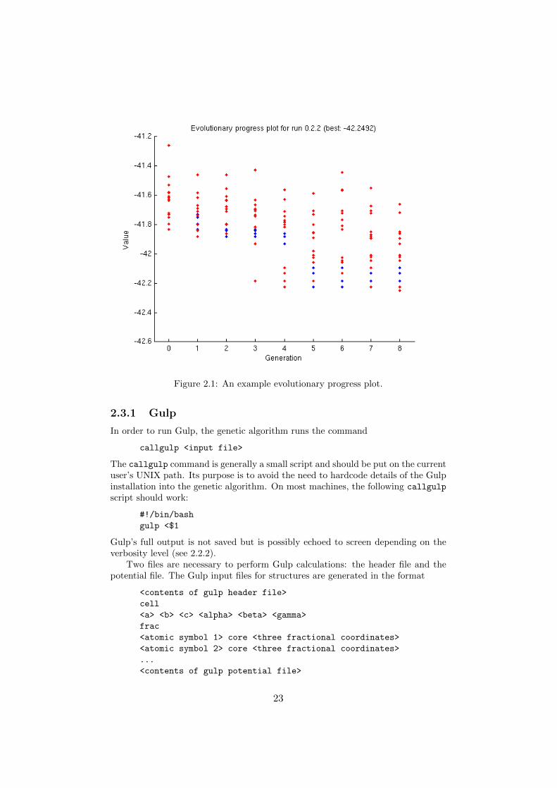
Figure 2.1: An example evolutionary progress plot.

2.3.1 Gulp

In order to run Gulp, the genetic algorithm runs the command

callgulp <input file>

The callgulp command is generally a small script and should be put on the currentuser’s UNIX path. Its purpose is to avoid the need to hardcode details of the Gulpinstallation into the genetic algorithm. On most machines, the following callgulp

script should work:

#!/bin/bash

gulp <$1

Gulp’s full output is not saved but is possibly echoed to screen depending on theverbosity level (see 2.2.2).

Two files are necessary to perform Gulp calculations: the header file and thepotential file. The Gulp input files for structures are generated in the format

<contents of gulp header file>

cell

<a> <c> <alpha> <beta> <gamma>

frac

<atomic symbol 1> core <three fractional coordinates>

<atomic symbol 2> core <three fractional coordinates>

...

<contents of gulp potential file>

23

where the tokens in brackets are not to be interpreted literally. Lines specifyingthe location of species’ shells are included if needed.

One should refer to the Gulp manual [1] for all the options available, but aGulp header file might look like the following:

opti conp conj

switch_minimiser bfgs gnorm 0.2

This tells Gulp to optimize both the lattice parameters and atomic positions ofthe structure under constant pressure. It will initially use a conjugate-gradientminimization routine but will switch to the Newton-Raphson BFGS method afterthe gradient norm falls below 0.2. This strategy of switching minimizers is usefulfor many systems.

There are also many ways to give Gulp an empirical potential. As an example,though, consider

lennard

C core C core 100470 64.464 0.000 8.5125

This is the Lennard-Jones potential used by Abraham and Probert to model carbon[4].

2.3.2 Vasp

Similarly to the callgulp script, a callvasp script is used to move the details ofa Vasp installation out of the Java code and into a shell script. The particularcommand run by the genetic algorithm is

callvasp <input directory>

The input directory is that containing the POSCAR, POTCAR, KPOINTS andINCAR files. So the callvasp script on many machines will look something like

#!/bin/bash

cd $1

vasp

The situation is slightly more complicated if the investigator wants to use e.g.the GridEngine job-queuing system. The script can not simply call qsub because thegenetic algorithm assumes that the energy calculation is complete when callvasp

returns. A solution is described in Appendix B. The user should check that theautomatically generated Vasp input files are satisfactorily parametrized [2].

2.3.3 LAMMPS

Similarly to with the other codes, a calllammps script is used by the GA to interactwith the LAMMPS code. The GA runs

calllammps <input directory>

where <input directory> is a directory holding lammps input files including onecalled in.min. The script should run LAMMPS and exit only once the calculationis finished. So, it probably looks something like

24

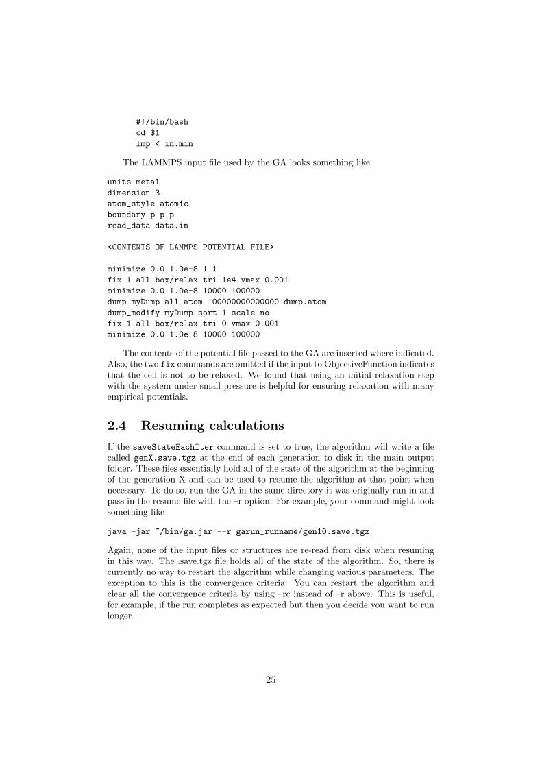
#!/bin/bash

cd $1

lmp < in.min

The LAMMPS input file used by the GA looks something like

units metal

dimension 3

atom_style atomic

boundary p p p

read_data data.in

<CONTENTS OF LAMMPS POTENTIAL FILE>

minimize 0.0 1.0e-8 1 1

fix 1 all box/relax tri 1e4 vmax 0.001

minimize 0.0 1.0e-8 10000 100000

dump myDump all atom 100000000000000 dump.atom

dump_modify myDump sort 1 scale no

fix 1 all box/relax tri 0 vmax 0.001

minimize 0.0 1.0e-8 10000 100000

The contents of the potential file passed to the GA are inserted where indicated.Also, the two fix commands are omitted if the input to ObjectiveFunction indicatesthat the cell is not to be relaxed. We found that using an initial relaxation stepwith the system under small pressure is helpful for ensuring relaxation with manyempirical potentials.

2.4 Resuming calculations

If the saveStateEachIter command is set to true, the algorithm will write a filecalled genX.save.tgz at the end of each generation to disk in the main outputfolder. These files essentially hold all of the state of the algorithm at the beginningof the generation X and can be used to resume the algorithm at that point whennecessary. To do so, run the GA in the same directory it was originally run in andpass in the resume file with the –r option. For example, your command might looksomething like

java -jar ~/bin/ga.jar --r garun_runname/gen10.save.tgz

Again, none of the input files or structures are re-read from disk when resumingin this way. The .save.tgz file holds all of the state of the algorithm. So, there iscurrently no way to restart the algorithm while changing various parameters. Theexception to this is the convergence criteria. You can restart the algorithm andclear all the convergence criteria by using –rc instead of –r above. This is useful,for example, if the run completes as expected but then you decide you want to runlonger.

25

2.5 Strategies

A number of general strategies for successful genetic algorithm runs have beennoticed. We will list and discuss some of them here.

There is a trade-off between the speed of convergence of the algorithm and thechance that it has found a global minimum since it is a search-based algorithm andneeds time to sample the space and then investigate the most promising regions.The sampling of the space is very important, so it is often best to start with aninitial population that is somewhat larger than subsequent generations.

The primary way we make a choice in the speed-certainty trade-off is by choos-ing a selection method. As mentioned previously, for a population of 20 organisms,a (5, 2) selection strongly favors the best organisms in a generation and will leadto quick convergence. However, we will occasionally see test systems where sucha parametrization improperly converges. A (20, 1) selection is generally preferablefor this reason.

A partial exception is for close-packed and metallic type structures. The al-gorithm generally finds the correct lattice for these quite quickly since the energydifference between lattices is much larger than differences in energy due to differ-ent site decorations. In this case the stronger selection may be appropriate as thegenetic information of better organisms is likely to be strictly better than that inhigher energy structures.

An important parameter to keep track of when varying the selection is numPromoted,the number of the best organisms which are automatically promoted from one gen-eration to the next. In particular, if numPromoted is greater than numParentsand there are no good organisms created in a generation, then the set of parentorganisms can be the same in the next generation.

Then, especially if numParents is small, it is likely that many of the offspringwill be similar to those which were unsuccessfully created from the same parents inthe previous generation. It is likely that the same set of parents will be promotedto the next generation and so on. Progress will stagnate. To avoid this situationit is almost always best to use both redundancy guards and choose a numParentsgreater than numPromoted.

It is best to scale randomly created structures in the initial generation to avolume as close as possible to the optimal volume. This is, of course, an unknown,but can often be estimated. This makes the hard constraints more meaningful andsignificantly improves the speed and chances of the local minimization. For systemswith many atoms, it may take a lot of tries to randomly generate structures, but ittakes much longer to perform an energy calculation on a poorly formed structure.Density optimization and the strictest hard constraints that do not limit the set ofpossible solutions should generally be used for similar reasons.

A sample input file which should work as a template for most systems may befound in Appendix C.

26

Chapter 3

Implementation

3.1 General strategy

The algorithm is implemented in Java and packaged as a Jar file.

3.2 Randomness

The genetic algorithm is a stochastic search method and often needs random num-bers. Here, we have used the PRNG that comes with Java. In particular, aninstance of java.util.Random is created by GAParameters and is accessible toother objects through its getRandom() method. It is important that all methodsuse this single PRNG. If methods each created their own Random object using thestandard method of seeding with the current time, repeated calls to fast algorithmswhich use randomness might have the same result.

Random numbers are often drawn from a distribution which is determined byuser input. If the input specification asks for an upper and lower bound, then thecorresponding distribution is uniform. If the input specification asks for a sigmaand mean, then the corresponding distribution is Gaussian.

3.3 The main loop

The main loop lives in GeneticAlgorithm.doGeneticAlgorithm. The functiontakes a GAParameters object which should already be “filled out”. Eventually, itreturns a Structure object containing the result.

So, until it has converged, the main loop is mostly concerned with turningparents into offspring using Variations. A full listing of the code is in AppendixA. Most of the steps will be explained more fully later, but a couple of things areworth noting now.

First, each organism with is added to the generation is developed, evaluated,and developed again. The primary task of development is to enforce the hardconstraints. It is necessary to develop an organism before the evaluation to avoidexpensive energy calculations on particularly poor candidate structures. However,it is also necessary to do certain things (e.g. redundancy checks, cell reduction)after the evaluation. A structure may relax out of the hard constraints during the

27

energy calculation. So, we end up developing a structure twice before it is addedto the offspring generation.

Secondly, we do not specify that a certain number of organisms be producedfrom specific Variations each generation. Instead, we specify the probability thata particular Variation will be used. In this way, the algorithm avoids becomingstuck in the case that one of the Variations can not produce successful offspring.(This could happen, for example, if the population had mostly converged so thatall organisms created by Slicer converge to a structure already in the generationand fail the redundancy check. We would want the mutation variations to pick upthe slack.)

However, the offspring of some Variations might be perfectly capable of pro-ducing viable offspring but less likely to do so. For example, the offspring of aPermutation will never fail the interatomic distance, but that of a StructureMut

often will. In cases like this, we would like to stay as close as possible to the speci-fied proportions. So, once a Variation is chosen, we use it to make new organismsuntil one is found which satisfies (at least) the pre-evaluation development.

3.4 ObjectiveFunction and Energy

ObjectiveFunction is an abstract class specifying, most notably, the evaluate

method. This method returns a Thread which has been started. When thethread exits, the energy calculation is assumed to be complete. A new instanceof the ObjectiveFunction is created for each energy calculation through a call toGAParameters. The abstract class also contains a counter to keep track of the num-ber of function evaluations it does. Classes extending ObjectiveFunction shouldincrement this counter when appropriate.

ObjectiveFunction is extended only by the EnergyPerAtom class, whose evaluatemethod returns the energy of a structure divided by the number of atoms in itscell. If the given StructureOrg already knows its value, this number is returned.Otherwise, the method must initiate a total energy calculation using an Energy.

The Energy interface specifies the getEnergy method and is implemented byGulpEnergy and VaspEnergy. These run the scripts callgulp and callvasp asdescribed in 2.3.

3.5 Genetic operators

3.5.1 Selection

Selection is an interface specifying the single method doSelection. It takes aninteger n and a Generation g and returns an array containing n members of g. Itis implemented only by ProbDistSelection whose behavior is described in 1.4.4,and the lone instance of which is a private member variable of GAParameters.

The doSelection method of ProbDistSelection calls findProbabilities

to get a mapping from structures to their normalized selection probabilities. Itrandomly selects and returns n structures based on the probabilities (assuming thatn is not greater than the size of the generation). The calculation of the probabilitiesthemselves is a straightforward implementation of the formulas described in themethodology, but special note should be taken of the fitnesses renormalization.

28

3.5.2 Variation

Variation is an interface implemented by Slicer, StructureMut, Permutation,and numStoichsMut. It specifies the doVariation method which takes two Generationsand a Selection and creates an Organism which may be added to the offspringGeneration. The variation objects themselves are straightforward implementationsof the methods described in Chapter 1.

3.5.3 Promotion

There is one instance of Promotion. It is a private variable of the GAParameters sin-gleton created when the “promotion” tag is read from the input file. Its doPromotionmethod is called at the beginning of each generation (line 22 in the main loop). Atthis point, it simply copies the top numPromoted organisms from the parent tothe offspring generation.

All other times when parents are used to create children are implemented asVariation objects. This is not a Variation since Variations only create a singleorganism at a time. A promotion variation would have to keep some state infor-mation about which organisms it had previously promoted, and this state wouldneed to be wiped clean each generation. This is possible, but it would fall some-what outside the intended purpose of Variation. Variation objects have directbiological analogies, whereas with Promotion, we have tried to improve upon thenatural process.

3.5.4 Development

Development is an interface specifying the single Boolean method doDevelop whichhas only been implemented by the StructureDev class. If specified, this class isused twice each time the algorithm creates a new organism.

The doDevelop method of the StructureDev class takes a single Organism andthe Generation of which it may be a member. It takes the Niggli reduced cell. Itthen checks, in order, that the organism satisfies the various hard constraints, sto-ichiometry constraints, redundancy guard checks, and the δValue rule.The methodreturns true to indicate that the organism developed successfully and false oth-erwise.

The Organism will be modified by Niggli cell reduction. The Generation willbe modified in two cases. If an Organism has already been relaxed but fails eitherthe δValue rule or the perGen redundancy check, we compare its value to that of theOrganism with which it conflicts. If the new Organism is better, the Development

manually removes the old one from the Generation and adds the new one. It thenreturns false to tell the calling method that we did not, effectively, find a newstructure which needs to be added to the Generation.

3.6 Organisms

3.6.1 Organism representation and StructureOrg

Organism is an abstract class which holds operations on a structure’s fitness, value,and ID. The ID is a unique number used to identify the Organism in the algorithm’soutput.

29

StructureOrg is an Organism and has a Structure. Most of the logic inStructureOrg.java is for the input and output of Cif files.

3.6.2 Generation and Structures

Generation is an abstract class which contains a Vector of Organism. It imple-ments the normalization of values into fitnesses as well as some basic statisticaloperations on its Organisms.

Structures is the extension of Generation used for the structure predictionproblem. The Structures class holds the perGen RedundancyGuard if it is in use.

New Generations are created by the main loop (line 18) through calls toGAParameters since it knows the type of Generation to use.

3.6.3 Initial population

Organisms are made by objects which implement StructureOrgCreator whichspecifies the single method StructureOrg makeOrganism(Generation). A StructureOrgCreator

is made by GAParameters when its input-file parser encounters the InitialPopulationtag. The new StructureOrgCreator and the number of organisms it is to be used tomake are stored in a mapping, Map<StructureOrgCreator,Integer> initialOrgCreators

in GAParameters. This map is used when the main loop calls getNewOrg duringthe first generation.

Notice that Organisms are developed, evaluated, and then developed again be-fore being added to the Generation and that this is done inside the Structures

constructor. Also notice that, although StructureOrgCreators only return oneOrganism at a time, they might need to know something about their previous ac-tions. For example, FromCifsSOCreator should only return any particular Structureonce. The general strategy in these cases is to create all possible StructureOrgson the first call, store them in a list, and remove them as they are used.

The StructureOrgCreator used to create a StructureOrg is stored in a mem-ber variable of that organism. The only purpose for this has to do with ini-tial generation creation using the parallelized algorithm. We want to use eachStructureOrgCreator to create a given number of Organisms for the first Generation.However, we only want to count those Organisms which successfully relax and de-velop. We need to keep track of the method used to create an Organism so that weknow which method to give the credit for its success.

3.6.4 Fitness and value

The difference between fitness and value is discussed in 1.4.2. Both numbers arestored as member variables of the Organism abstract class. They are initialized tonull indicating that they have not yet been calculated. The value of an organismis calculated by the ObjectiveFunction on line 37 of the main loop (see 3.3). Thecalculation of fitness is done by the Generation.

An Organism knows whether or not its value and fitness have been calcu-lated. The Boolean methods knowsFitness and knowsValue is used by objects(e.g. StructureDev) which need to act on this information.

30

3.7 Convergence

The decision whether or not to halt the algorithm is made at the end of eachgeneration. It is mediated by classes implementing the ConvergenceCriterion

interface which specifies the Boolean converged(Generation) method. By con-vention, all of these classes end in “CC”. They are, FoundStructureCC.java,NumFunctionEvalsCC.java, NumGensCC.java, NumGensWOImprCC.java and ValueAchievedCC.java.

ConvergenceCriterions are created by GAParameters during argument pars-ing. They are added to a list. At the end of each generation, the evaluate methodof each object in this list is called by converged in GeneticAlgorithm.java, andif any return true, the algorithm is halted.

3.8 Input and parameters

GAParameters is a singleton class which is responsible for parsing most of thecommand line and input file options. It passes the ones which are particular to acertain algorithm on to that algorithm and stores the rest. Most of the dirty workis contained in GAParameters.setArgs. The command-line and input-file optionsare parsed into separate Map<String,String[]> and then combined such that thecommand-line arguments take precedence.

Next is a long chain of else ifs in which there is one entry to handle eachflag. For example, a command line option might be:

--objectiveFunction epa gulp gulpheader gulppotl true

An entry in the chain recognizes the first token, ’–objectiveFunction’. It readsthe next token, ’epa,’ to decide that it should make an EnergyPerAtom objectivefunction. The rest of the arguments, ’gulp gulpheader gulppotl true,’ are passed tothe EnergyPerAtom constructor. The EnergyPerAtom constructor reads the firsttoken, ’gulp,’ to see that it should use a GULP energy function, which happens tobe called GulpEnergy. The rest of the arguments, ’gulpheader gulppotl true,’ arepassed on to GulpEnergy where they are parsed and stored. In this way, it is notnecessary for GAParameters to be able to deal with all of the parameters of thewhole program, but only the “top-level” ones.

Some common idioms are used repeatedly for parsing input options, especiallyin the “else-if chain” in GAParameters and in the constructors of algorithms whichneed parameters. See the code in 3.11.1 for examples.

3.9 Parallelization

Parallelization of the algorithm within a single generation is relatively straightfor-ward. Variations can be used to quickly create a generation’s worth of offspring, andthose offsprings’ energy calculations can be run concurrently in separate threads.See lines 37 through 43 in the main loop.

The only problem with this occurs when one offspring fails a development stage.In this case, we can end up having less organisms in a generation than we expectedto. In the unlikely case that very few offspring are successful, the algorithm couldfail to run normally. However, creating one or two more organisms after findingthat some fail would be an inefficient use of resources.

31

Fortunately, having a slightly smaller offspring generation will rarely be a prob-lem. So the parallelization code needs to take the minimum number of organismsacceptable in any generation as a parameter. If this number is, say, ninety percentof a full generation, then the algorithm will run normally and efficiently. If a newgeneration falls short of the given threshold, we simply compute more structuresuntil we have enough.

We also take as a parameter the number of energy calculations to run concur-rently. We start this many at a time and wait for them all to finish before beginningmore.

3.10 Description of files

Descriptions of each of the files follow.

• ConvergenceCriterion.java

ConvergenceCriterion is an interface specifying the Boolean method converged(Generation).Each ConvergenceCriterion in use should be called by the algorithm exactlyonce per generation. It will return true if the population is determined tohave converged at which point the algorithm is stopped. By convention,classes implementing ConvergenceCriterion end in “CC”.

• CrystalGA.java

CrystalGA contains the methods that any user of the algorithm will call,whether that user is external code or the command line.

• DatabaseSOCreator.java

DatabaseSOCreator implements StructureOrgCreator. It creates Structure-Orgs from a database of prototype structures.

• Development.java

The Development interface is implemented by methods which oversee the“growing up” of an organism by implementing doDevelop. If the organismis obviously unfit (hard constraints), doDevelop may return false, and theorganism should not be considered any further. doDevelop may modify theOrganism (e.g. structure relaxation), but should not modify the Generation.

• Energy.java

Classes which implement the Energy interface can compute the total latticeenergy of a StructureOrg. They’re generally wrappers which call an exter-nal code. They are most often not ObjectiveFunctions, but are used byObjectiveFunctions (e.g. EnergyPerAtom).

• EnergyPerAtom.java

EnergyPerAtom is an ObjectiveFunction. It uses an Energy object to com-pute the energy of a StructureOrg and then normalizes that by the numberof atoms in the StructureOrg to get the Organisms’s value. Notice thatthere is no chemical potential involved, so this ObjectiveFunction is reallyonly physically useful when we fix the stoichiometry.

32

• FoundStructureCC.java

FoundStructureCC is a ConvergenceCriterion which indicates convergencewhen there is a member of the current generation which is the same as a givenStructure. The target Structure is given as a Cif file and the matching isdone using a RedundancyGuard which calls a StructureFitter internally.

• FromCifsSOCreator.java

FromCifsSOCreator implements StructureOrgCreator. It is given a direc-tory, and it creates StructureOrgs from all Cif files in the directory.

• GAParameters.java

GAParameters is a singleton class which is responsible for parsing and storingmost of the command line and input file options. It passes the ones whichare particular to a certain algorithm on to that algorithm and stores the rest.The main algorithms and the Population are also owned by GAParameterssince GAParameters has all the info about what particular algorithms shouldbe used. The result of this is that the algorithms and Population are kindof pseudo-singletons in that they should only need to be accessed throughGAParameters’s getters.

• GARecord.java

GARecord is a singleton class which keeps a record of the status and progressof the genetic algorithm. Its function finishGen is called after each gener-ation and is responsible for outputting results to console and disk. It takescare of other tasks which require a sense of history, e.g. counting the numberof generations since the algorithm made improvement.

• GAUtils.java

GAUtils holds a variety of general utility functions as well as the usage state-ment.

• Generation.java

Generation contains a Vector of Organisms which are treated logically asa generation. It also implements a number of operations on that group suchas calculation of fitnesses from values. A generation is not an evolving pop-ulation: after its creation, it rarely gains or loses members.

• GeneticAlgorithm.java

This holds the main genetic algorithm. It contains the evolutionary strategyin abstract form. For crystal structure prediction, client code should callCrystalGA.crystalGA(). See also Appendix A.

• GulpEnergy.java

GulpEnergy computes the total energy of a StructureOrg using GULP andthe given potential. It contains all of the methods and utilities that arespecific to GULP.

• ManualSOCreator.java

ManualSOCreator allows for structures to be added by code which uses thegenetic algorithm. That code should call GAParameters.setSeedStructuresbefore beginning the algorithm.

33

• NumFunctionEvalsCC.java

NumFunctionEvalsCC implements ConvergenceCriterion. It indicates thatthe algorithm has converged after a certain number of ObjectiveFunction

evaluations have been done. Notice that keeping track of the number ofevaluations is done by the ObjectiveFunction itself.

• NumGensCC.java

NumGensCC implements ConvergenceCriterion. It indicates that the al-gorithm has converged when the algorithm has run for a given number ofgenerations.

• NumGensWOImprCC.java

NumGensWOImprCC implements ConvergenceCriterion. It indicates that thealgorithm has converged when the algorithm has run for a given number ofgenerations without improving its best solution.

• NumStoichsMut.java

NumStoichsMut implements Variation. It creates an offspring StructureOrg

from a parent by adding or removing a randomly chosen number of stoi-chiometries worth of species.

• ObjectiveFunction.java

ObjectiveFunction is an abstract class which specifies the interface to func-tion we want to minimize.

• Organism.java

Organism is the abstract class which represents members of a Generation inthe genetic algorithm. It is implemented by e.g. StructureOrg. It maintainsthe parts of an Organism not specifically related to the structure predictionproblem such as value, fitness, and organism ID.

• Permutation.java

Permutation is a Variation operation which creates an offspring from oneparent by randomly swapping some of its atoms. The number of swaps isnormally distributed with mean and standard deviation taken by the functionas arguments.

• ProbDistSelection.java

Contains the algorithm for random selection of Organisms as described in1.4.4.

• Promotion.java

Promotion “promotes” some number of the best organisms in one generationdirectly to the next.

• RandomSOCreator.java

RandomSOCreator implements StructureOrgCreator. It creates StructureOrgsas described in 2.1.1.

• RedundancyGuard.java

RedundancyGuard is used by the algorithm to avoid considering identicalStructureOrgs more than once. It stores a Map of all Structures “seen” to

34

their Organism IDs. Then, other algorithms (e.g. StructureDev) may checkOrganisms against the list of those already seen. Comparisons are done firstby a direct comparison of lattice parameters and atomic positions and second,if necessary, by the slower but more accurate StructureFitter.

• ResumeSOCreator.java

ResumeSOCreator implements StructureOrgCreator. It creates new Struc-tureOrgs from the output of a previous GA run and is generally used for thelimited resume-type functionality described in 2.1.1.

• Selection.java

Selection is an interface to objects which take a Generation and an integer,n, and returns a vector of n organisms from the Generation. It assumes thatfitnesses have already been calculated.

• Slicer.java

Slicer is a Variation operation. It implements the algorithm described in1.4.5.

• StructureDev.java

StructureDev implements Development and is the Development operationgenerally used with StructureOrgs. See 1.4.8.

• StructureMut.java

StructureMut is a Variation operation which acts on StructureOrg organ-isms. See 1.4.5.

• StructureOrg.java

StructureOrg extends Organism and has a Structure. It is the type ofOrganism generally used by the genetic algorithm for the crystal structureprediction problem.

• StructureOrgCreator.java

StructureOrgCreator is an interface to objects which create StructureOrgs,generally for use in the initial population.

• Structures.java

Structures extends Generation and has list of StructureOrg. It is thetype of Generation generally used by the genetic algorithm for the crystalstructure prediction problem.

• ValueAchievedCC.java

ValueAchievedCC is a ConvergenceCriterion which indicates convergencewhen there is at least one member of the current generation with a value lessthan or equal to a given target value.

• Variation.java

A Variation takes a pair of generations and considers them in creatingan Organism to be added to the offspring generation. Neither Generation

should be modified. Application of Variations, along with Promotion, arehow a new Generation is created from a parent Generation.

• VaspEnergy.java

VaspEnergy implements Energy. It computes the total energy of a StructureOrgusing Vasp and the given pseudopotentials.

35

3.11 Modifying the code

3.11.1 Example: adding a parameter

Recall that the algorithm can change behavior when it thinks it has converged.Suppose we want to add the parameter endGameNumGens which indicates thenumber of generations without improvement the algorithm will run before it decidesit has probably converged. The line we add to the input file will look somethinglike:

endGameNumGens 6

This parameter applies to the algorithm as a whole rather than to any particularsubroutine, so it will live in GAParameters. We add the following private variableto GAParameters:

private int endGameNumGens = 50;

with a very conservative default value. Then, we add it to the chain of else-ifs inGAParameters.setArgs:

else if (flag.equalsIgnoreCase(‘‘--endgameNumGens’’))

endGameNumGens = Integer.parseInt(getValues(flag)[0]);

The easiest way to do this part is probably to copy and paste the code from a pre-existing parameter. Notice the “--” which is necessary whether the flag was passedin on the command line or from the input file. We are not really validating the formof the input, but the default error that Integer.parseInt or Double.parseDoublewill throw if given malformed input is satisfactory.

Now, the endGame check is implemented in GARecord which is responsiblefor recording what has happened over past generations. We need to make theparameter available to GARecord, so we add the following getter at the bottom ofGAParameters:

public int getEndGameNumGens() {

return endGameNumGens;

}

We have adhered to the convention of naming getters as “get” plus the name ofthe relevant parameter. Now we may access the parameter from GARecord (oranywhere else) using

int n = GAParameters.getParams().getEndGameNumGens();

Finally, we are sure to add an entry to the usage statement in GAUtils and thetoString method of GAParameters.

3.11.2 Example: testing new variations

It is possible and often helpful to test a Variation without performing a full runof the genetic algorithm. Furthermore, the code to do so is a good example of howmany of the objects we have discussed fit together. The following is an adaptedversion of Slicer’s main method:

36

1 public static void main(String[] args) {2 GAParameters params = GAParameters.getParams();

3 Structure p1 = StructureOrg.parseCif(new File(‘‘parent1.cif’’));

4 Structure p2 = StructureOrg.parseCif(new File(‘‘parent2.cif’’));

5

6 Generation parents = params.makeEmptyGeneration();

7 parents.addOrganism(new StructureOrg(dense1));

8 parents.addOrganism(new StructureOrg(dense2));

9

10 String[] vArgs = {‘‘0.5’’, ‘‘0.0’’, ‘‘0’’, ‘‘0.00’’, ‘‘1’’, ‘‘2’’};11 Variation p = new Slicer(vArgs);

12 String[] selArgs = {‘‘2’’, ‘‘0’’};13 Selection sel = new ProbDistSelection(selArgs);

14

15 StructureOrg o = (StructureOrg)p.doVariation(parents, null, sel);

16 GAUtils.writeStringToFile(o.getCIF(), new File(‘‘out.cif’’), false);

17 }

The variation itself happens on line 15. It requires a parents Generation and aSelection to act. Setting the second argument to null indicates that no develop-ment will be done. The creation of the Variation object itself is on lines 10 and11. The Selection is made on lines 12 and 13. Clearly, it needs to select from thetop two organisms in the generation, but the selection power is irrelevant.

Now we must create the parents Generation. It will contain the two parentorganisms which are loaded from files in lines 3 and 4. The Generation itself iscreated through the call on line 6 and the two parents are added to in on lines 7and 8. Line 2 is an idiom which occurs many times in the code. We are accessingand storing the parameters singleton for repeated use.

Finally, on line 16, the Cif file of the offspring is written to disk.

37

Appendix A

Main loop

A partial listing of GeneticAlgorithm.java including the main loop follows. See3.3 for a discussion.

1 public static Organism doGeneticAlgorithm(GAParameters params) {2 GARecord record = GARecord.getRecord();

3 int verbosity = params.getVerbosity();

4

5 // Create the objects for the algorithms

6 Selection sel = params.getSelection();

7 Development dev = params.getDevelopment();

8 Promotion pro = params.getPromotion();

9

10 // Create the initial population

11 Generation parents = null;

12 Generation offspring = null;

13

14 // the main algorithm loop:

15 while (!converged(offspring)) {16 // the wheel of life turns

17 parents = offspring;

18 offspring = GAParameters.getParams().makeEmptyGeneration();

19

20 // do promotions (except for the first generation)

21 if (GARecord.getRecord().getGenNum() != 0)

22 pro.doPromotion(parents, offspring);

23

24 // make the offspring generation

25 while (!madeEnough(offspring)) {26 List<Organism> organisms = new ArrayList<Organism>();

27 List<Thread> threads = new ArrayList<Thread>();

28

29 for (int i = 0; i < params.getNumCalcsInParallel(); i++) {30 // make a new organism

31 Organism newOrg = getNewOrg(parents, offspring, sel);

32 if (newOrg == null)

38

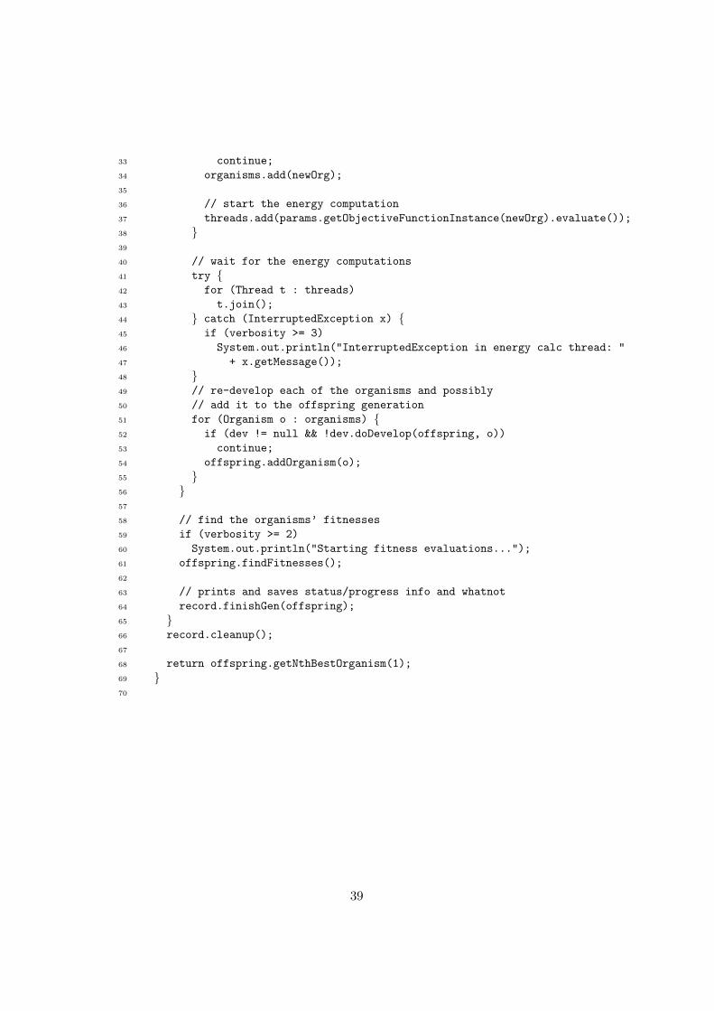
33 continue;

34 organisms.add(newOrg);

35

36 // start the energy computation

37 threads.add(params.getObjectiveFunctionInstance(newOrg).evaluate());

38 }39

40 // wait for the energy computations

41 try {42 for (Thread t : threads)

43 t.join();

44 } catch (InterruptedException x) {45 if (verbosity >= 3)

46 System.out.println("InterruptedException in energy calc thread: "

47 + x.getMessage());

48 }49 // re-develop each of the organisms and possibly

50 // add it to the offspring generation

51 for (Organism o : organisms) {52 if (dev != null && !dev.doDevelop(offspring, o))

53 continue;

54 offspring.addOrganism(o);

55 }56 }57

58 // find the organisms’ fitnesses

59 if (verbosity >= 2)

60 System.out.println("Starting fitness evaluations...");

61 offspring.findFitnesses();

62

63 // prints and saves status/progress info and whatnot

64 record.finishGen(offspring);

65 }66 record.cleanup();

67

68 return offspring.getNthBestOrganism(1);

69 }70

39

Appendix B

Using GridEngine and Vasp

To perform an energy calculation using Vasp, the genetic algorithm runs the com-mand

callvasp <input file directory>

It expects that when this script is done running, the vasprun.xml file is fullywritten and ready for parsing. That is, the callvasp script can not end until theVasp calculation is complete.

In order to submit jobs to a GridEngine queue, the qsub command is used.However, qsub exits immediately. The following callvasp script is a work-aroundfor this issue.

1 #!/bin/bash

2 cd $1

3 qsubandpoll /home/wtipton/bin/submitjob

where qsubandpoll is a script on the user’s path and the path to submitjob willchange.

The heart of this solution is the qsubandpoll script. It gives each job a uniquerandom name, submits the job to the queue, and then checks the output of qstat atregular intervals to determine when the job has finished. A listing of qsubandpollfollows:

1 #!/bin/bash

2

3 INTERVAL=1

4 TEMP=‘mktemp‘

5 UNIQUENAME=‘echo $TEMP|sed ’s/tmptmp_//’‘

6

7 qsub -N $UNIQUENAME $1

8 while : ; do

9 sleep $INTERVAL

10 MATCH=‘qstat | grep -o $UNIQUENAME‘

11 if [ "$MATCH" == "" ]; then

12 break

13 fi

14 done

40

15

16 rm $TEMP

Notice that on lines 4, 5 and 10, the outer ‘ characters are backticks.Finally, submitjob is a normal qsub script. Keeping in mind that the genetic

algorithm expects vasprun.xml to be available in the output, submitjob mightlook something like

1 #$ -o vasp.out

2

3 /share/apps/aflow173 -vasp /share/apps/vasp/vasp.core2.64

4 gzip -d vasprun.xml.relax2.gz

5 mv vasprun.xml.relax2 vasprun.xml

41

Appendix C

Example input file

Please see the QuickStart guide located at http://gasp.mse.cornell.edu/manual.html.

It includes an input file for a Lennard-Jones Gulp run. It errs on the sideof conservativism and may be used as a basic template for future runs. Recallthat lines beginning with ”#” are ignored, everything (except sometimes atomicsymbols) is case-insensitive, and units are generally eV, Angstroms and degrees.Detailed descriptions of options are given in 2.1.1.

42

http://gasp.mse.cornell.edu/manual.html

http://gasp.mse.cornell.edu/manual.html

Appendix D

Scripts for testingparameters

In order to evaluate the dependence of the success of the algorithm on its pa-rameters, three scripts were used to repeatedly run the algorithm while varying aparameter, to parse the output for the number of energy calculations needed, andto visualize the result. The first of these follows.

1 #!/bin/bash

2

3 NUMRUNSPERVALUE=20

4 GA_IN_TEMPLATE=/home/wtipton/testing/ljc_newt/input_template

5 INITIALVALUE=0.5

6 FINALVALUE=1

7 INCREMENT=0.1

8 GA="/home/wtipton/projects/ga_for_crystals/ga.jar"

9

10 #### Shouldn’t be necessary to change below here ####

11 GA_IN_KEY_TO_CHANGE=CHANGEME

12 mkdir runs || exit

13 cd runs

14

15 for VALUE in ‘seq -w $INITIALVALUE $INCREMENT $FINALVALUE‘

16 do

17 # make the input file for this value of the varied parameter

18 GA_IN="ga_in_$VALUE"

19 sed "s/$GA_IN_KEY_TO_CHANGE/$VALUE/" "$GA_IN_TEMPLATE" >"$GA_IN"

20

21 # run the GA NUMRUNSPERVALUE times for this value

22 for RUN in ‘seq 1 $NUMRUNSPERVALUE‘

23 do

24 echo "Starting run $RUN of value $VALUE"

25 #replace the outDirName

26 sed -i ’s/.*outDirName.*//’ "$GA_IN"

27 echo outDirName "$VALUE.$RUN" >>$GA_IN

28 #run the GA

43

29 java -jar $GA --f "$GA_IN" | tee "output.$VALUE.$RUN"

30 done

31 done

This script runs the genetic algorithm repeatedly while varying a parameter. Theuser should only have to change the variables at the top of the script and the inputtemplate for any test. The input template should be a regular input file with thevalue that is going to be varied set to “CHANGEME.” The algorithm will be runwith that value set to each of the values between the initial and final values given.Make sure to set reasonable convergence criteria.

The second script, parse results.sh, should be run from the same directoryas the first. It parses the directory structure created by the first script and outputsa file called “results.”

1 #!/bin/bash

2

3 rm results

4 cd runs

5 ls output* | while read i ; do

6 NUMCALCS=‘cat "$i" | tail -1 | cut -d ’ ’ -f 7‘

7 VALUE=‘echo $i|sed ’s/output\.//’ | sed ’s/\.[^.]*$//’ | sed ’s/ //g’‘

8 echo $VALUE $NUMCALCS >>../results

9 done

There is one line in the results file for each run of the genetic algorithm. Oneach line are two numbers: the value of the parameter and the number of energycalculations, respectively. The following Matlab script, testgraphs.m, takes thename of the results file, parses it and graphs the results.

1 function testgraphs(filename)

2

3 % read in ourFileName

4 fid = fopen(filename);

5 C = textscan(fid, ’%s’, ’delimiter’, ’\n’);

6 fclose(fid);

7 lines = C{1};

8

9 % initialize data structures

10 values = [];

11 numcalcs = [];

12

13 % read in the data

14 for i = 1:length(lines)

15 line = sscanf(lines{i}, ’%f’);

16 if (numel(line) ~= 2)

17 continue

18 end

19 values(end+1) = line(1);

20 numcalcs(end+1) = line(2);

21

22 end

44

23

24 % averages

25 avgCalcs=[];

26 stddevs=[];

27 for i = unique(values)

28 currentCalcs = nonzeros(numcalcs .* (values == i));

29 avgCalcs(end+1) = median(currentCalcs);

30 %avgCalcs(end+1) = mean(currentCalcs);

31 stddevs(end+1) = std(currentCalcs);

32 end

33

34 % plot it

35 hold on

36 errorbar(unique(values), avgCalcs,stddevs,’r’);

37 plot(values, numcalcs, ’ .’);

38 hold off

39 xlabel(’value’);

40 ylabel(’num calcs’);

41 title([’stuff’]);

45

References

[1] Gulp manual. https://www.ivec.org/gulp/help/manuals.html.

[2] Vasp manual. http://cms.mpi.univie.ac.at/vasp/vasp/vasp.html.

[3] Vics-ii: A crystal structure visualization tool. http://www.geocities.jp/

kmo_mma/crystal/en/vics.html.

[4] N. L. Abraham, A periodic genetic algorithm with real-space representationfor crystal structure and polymorph prediction, Physical Review B, 73 (2006).

[5] T. S. Bush, Evolutionary programming techniques for predicting inorganiccrystal structures, J. Mater. Chem., 5 (1995).

[6] G. Ceder, Data-mining-driven quantum mechanics for the prediction of struc-ture, MRS Bulletin, 31 (2006).

[7] D. M. Deaven, Molecular geometry optimization with a genetic algorithm,Physical Review Letters, 75 (1995).

[8] C. W. Glass, Uspex–evolutionary crystal structure prediction, ComputerPhysics Communications, 175 (2006).

[9] R. L. Johnston, Evolving better nanoparticles: Genetic algorithms for opti-mising cluster geometries, Dalton Trans., (2003).

[10] I. Krivy, A unified algorithm for determining the reduced (niggli) cell, ActaCrystallographica, A32 (1976).

[11] A. O. Lyakhov, A. R. Oganov, and M. Valle, Crystal Structure Predic-tion Using Evolutionary Approach, Wiley-VCH Verlag GmbH & Co. KGaA,2010, pp. 147–180.

[12] A. R. Oganov, Crystal structure prediction using ab initio evolutionary tech-niques: Principles and applications, Journal of Chemical Physics, 124 (2006).

[13] B. C. Revard, W. W. Tipton, and R. G. Hennig, Structure and stabil-ity prediction of compounds with evolutionary algorithms, Topics in CurrentChemistry, Springer Berlin Heidelberg, 2014, pp. 1–42.

[14] W. W. Tipton and R. G. Hennig, A grand canonical genetic algorithmfor the prediction of multi-component phase diagrams and testing of empiricalpotentials, Journal of Physics: Condensed Matter, 25 (2013), p. 495401.

[15] G. Trimarchi, Global space-group optimization problem: Finding the stablestcrystal structure without constraints, Physical Review B, 75 (2007).

[16] S. M. Woodley, The prediction of inorganic crystal structures using a geneticalgorithm and energy minimisation, PCCP, 1 (1999).

46

https://www.ivec.org/gulp/help/manuals.html

http://cms.mpi.univie.ac.at/vasp/vasp/vasp.html

http://www.geocities.jp/kmo_mma/crystal/en/vics.html

http://www.geocities.jp/kmo_mma/crystal/en/vics.html

gasp: the genetic algorithm for structure and … the genetic algorithm for structure and phase...

Documents