gasoline price changes and the petroleum industry: an update
TRANSCRIPT
Federal Trade CommissionBureau of Economics
Gasoline Price Changesand the PetroleumIndustry: An Update
An FTC Staff StudySeptember 2011


Federal Trade Commission
JON LEIBOWITZ Chairman WILLIAM E. KOVACIC Commissioner J. THOMAS ROSCH Commissioner EDITH RAMIREZ Commissioner JULIE SIMONE BRILL Commissioner
Bureau of Economics Joseph Farrell Director Alison Oldale Deputy Director for Antitrust Paul A. Pautler Deputy Director for Consumer Protection Pauline M. Ippolito Deputy Director for R&D and Operations Timothy A. Deyak Associate Director for Antitrust Louis Silvia Assistant Director for Antitrust I Michael G. Vita Assistant Director for Antitrust II David R. Schmidt Assistant Director for Applied Research and Outreach Janis K. Pappalardo Assistant Director for Consumer Protection
This is a report of the Bureau of Economics of the Federal Trade Commission. The views expressed in this report are those of the staff and do not necessarily represent the views of the Federal Trade Commission or any individual Commissioner. The Commission has voted to authorize staff to publish this report.


Acknowledgments
This report was prepared by the Bureau of Economics under the supervision of Joseph Farrell, Director; Howard Shelanski, Former Deputy Director; Tim Deyak, Acting Deputy Director; and Louis Silvia, Assistant Director. Bureau Economists who researched and drafted this report were Julie A. Carlson, Matthew Chesnes, Jeffrey H. Fischer, Geary Gessler, David W. Meyer, Christopher T. Taylor, Nathan E. Wilson, and Paul R. Zimmerman. Bureau Research Analysts who worked on this project were Amanda Kalamar and Elisabeth Murphy. Bureau Research Analyst Joseph Remy designed the cover.
Bureau of Economics staff also acknowledge the helpful comments and suggestions on a draft of the report by Peter Richman of the Bureau of Competition.
Clip art on the cover were obtained under license from www.thinkstockphotos.com.


EXECUTIVE SUMMARY
Between early September 2010 and late June 2011, crude oil and gasoline prices increased sharply. During that time the U.S. weekly average gasoline price increased $0.89 per gallon, from $2.68 to $3.57. These higher prices had a significant impact on U.S. consumers, potentially costing the average U.S. household around $60 per month. Since consumers reduce gasoline consumption by relatively small amounts as gasoline prices increase, that is around $60 less that consumers can save or spend on other goods each month, or about 1.5% of their average monthly expenditures, a significant amount for American families, especially in today’s economy. Even though prices have fallen somewhat from their high in the spring, they remain high by historical standards.
Because of the importance of energy prices to U.S. consumers, the Federal Trade Commission (FTC) has long had strong policy and enforcement interests in competition in the petroleum industry. In 2004 and 2005, the FTC published two reports that looked at general trends in the industry. This Report builds on those and focuses on gasoline prices and on changes in the petroleum industry between 2005 and early 2011. In June 2011, the FTC also opened an investigation relating largely to refineries to determine whether certain petroleum market participants have engaged or are engaging in anticompetitive, manipulative, or fraudulent practices that may violate the laws the Commission enforces, potentially allowing them to raise prices for American consumers.
Crude Oil Prices Drive U.S. Gasoline Prices
Crude oil prices continue to be the main driver of gasoline prices. Crude oil prices since 2005 have changed due to shifts in both world-wide demand and supply. While demand fell during the recent global recession, overall, consumption increased by almost 7% between 2004 and 2010. Crude oil demand from North America, Europe, Japan and Korea fell since 2004. In contrast, crude oil consumption increased in many developing countries. Crude oil consumption in China has been particularly strong, growing by 46%. This increase in demand has put upward pressure on crude oil prices.
World oil production has also increased over the years, with additional supply somewhat moderating the upward price pressure. Currently, over 70% of the world’s proven oil reserves are in Organization of Petroleum Exporting Countries (OPEC) member countries. OPEC attempts to maintain the price of oil by limiting output and assigning quotas. These actions by OPEC would be a criminal price fixing violation of the U.S. antitrust laws if done by private firms. OPEC’s production increased at a slower rate than non-OPEC production between 1974 and 2010. As a result, its share of global production has fallen from 54% to 42% even though its share of reserves has increased to over 70%. Recent economic research suggests that OPEC has some ability to affect prices, but that OPEC’s effectiveness as a cartel is limited. The largest increases in non-OPEC supply came from the United States, Russia, and Azerbaijan. Canada also significantly increased production due to the development of its oil sands reserves.

ii
Other Factors Relating to Gasoline Prices
Factors other than crude oil prices have also played significant roles in gasoline price changes at times since 2005. The loss of refinery capacity and disruptions of major crude and product pipelines due to the 2005 hurricanes led to large gasoline price spikes throughout the nation. Gasoline prices also increased significantly relative to crude oil costs in mid-2006 and mid-2007. In that case, the increase in the spread between crude oil and gasoline prices was due to several factors, including increased demand (in particular, the seasonal effects of the summer driving season), higher prices for ethanol, effectively reduced refinery capabilities due to the transition from methyl tertiary butyl ether (MTBE) to ethanol, and refinery outages, including lingering effects from the 2005 hurricanes. Gasoline demand fell during the recent recession. As a result of reduced demand, relaxed refinery constraints, and lower ethanol prices, gasoline prices generally remained low relative to crude oil prices between 2008 and early 2011.
There have been minor changes in the market structure for the refining and marketing of gasoline since 2005. While there was a small decrease in the number of U.S. refineries, overall refinery capacity increased by 3.6%. Fewer refineries changed hands than in previous years. Finally, refiners appear to be less integrated into gasoline retailing after several large refiners divested part of their retail operations.
Rockets and Feathers: The Speed of Gasoline Price Adjustments
Since 2005, economists have conducted additional research on how crude oil and gasoline prices adjust over time. One observation is that changes in crude oil prices are not instantly reflected in changes in spot or wholesale gasoline prices, and changes in those prices are not instantly reflected in retail prices. Rather, prices further down the supply chain adjust with lags. These lags vary for different levels of the supply chain, and also vary geographically. For example, changes in crude oil prices in August 2011 may not be fully reflected in changed retail gasoline prices until sometime in September.
One area of this line of research examines differences in the rate that these price changes are passed through when prices are increasing versus when they are decreasing. Recent studies indicate that retail gasoline prices react faster when prices are increasing than when they are decreasing. This phenomenon is popularly referred to as “rockets and feathers” because prices are said to go up like a rocket but fall like a feather. More formally, it is known as “asymmetric price adjustment” or “asymmetric pass-through.” There is less agreement on whether this phenomenon exists for other levels of the supply chain.
The causes of asymmetric pass-through in retail to wholesale price relationships are not fully understood. Researchers have suggested a number of potential causes. The explanation currently with the most support is that consumers search for lower cost gasoline more intensely when prices are rising than when they are falling. As a result, gas station owners do not face as much competitive pressure as prices fall and are less compelled to reduce price. While there is some evidence that consumer search intensity is different when prices are increasing as opposed to decreasing, it is not clear why search costs would vary across cities which display differing degrees of price asymmetry. The consumer welfare effects of asymmetric pass-through may receive further examination from the Commission in the future.

Table of Contents EXECUTIVE SUMMARY ........................................................................................................... i I. INTRODUCTION.......................................................................................................... 1 II. U.S. GASOLINE PRICES SINCE 2005 ...................................................................... 5
A. Recent History of National Average Gasoline Prices ................................................. 5
B. Recent Developments Affecting Crude Oil Prices ...................................................... 6
1. World Crude Oil Demand ............................................................................................ 6
2. World Crude Oil Supply .............................................................................................. 8
3. Futures Market Trading and Crude Oil Prices. ...................................................... 17
C. Other Factors Associated with Gasoline Price Changes .......................................... 23
1. The 2005 Hurricanes................................................................................................... 24
2. The 2006 and 2007 Summer Price Spikes ................................................................. 25
3. Recent Structural Trends in U.S. Refining ............................................................... 26
4. Recent Structural Changes in U.S. Gasoline Distribution ...................................... 30
a. Wholesale Concentration .......................................................................................... 31
b. Vertical Integration .................................................................................................... 31
5. Gasoline Imports ......................................................................................................... 33
III. GASOLINE PRICE ADJUSTMENTS: SOME NEW LEARNING ....................... 35 A. Local Differences in Retail Price Adjustment: An Example from the FTC Gasoline
Price Monitoring Project ............................................................................................. 36
B. Lags in Gasoline Price Adjustments .......................................................................... 38
C. New Learning on Pattern Asymmetry and Price Cycling ........................................ 39
D. Consumer Welfare Effects of Asymmetric Pass-Through and Price Cycling ........ 43
E. Future Work on Asymmetric Pass-Through ............................................................. 44
TABLES....................................................................................................................................... 47

I. INTRODUCTION
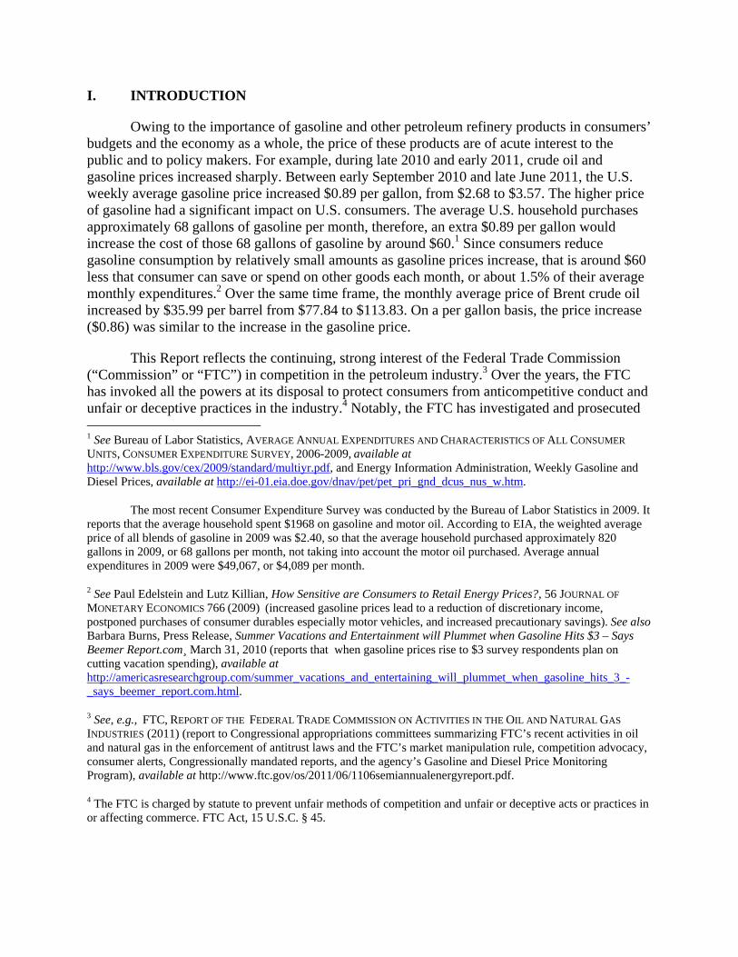
Owing to the importance of gasoline and other petroleum refinery products in consumers’ budgets and the economy as a whole, the price of these products are of acute interest to the public and to policy makers. For example, during late 2010 and early 2011, crude oil and gasoline prices increased sharply. Between early September 2010 and late June 2011, the U.S. weekly average gasoline price increased $0.89 per gallon, from $2.68 to $3.57. The higher price of gasoline had a significant impact on U.S. consumers. The average U.S. household purchases approximately 68 gallons of gasoline per month, therefore, an extra $0.89 per gallon would increase the cost of those 68 gallons of gasoline by around $60.1 Since consumers reduce gasoline consumption by relatively small amounts as gasoline prices increase, that is around $60 less that consumer can save or spend on other goods each month, or about 1.5% of their average monthly expenditures.2 Over the same time frame, the monthly average price of Brent crude oil increased by $35.99 per barrel from $77.84 to $113.83. On a per gallon basis, the price increase ($0.86) was similar to the increase in the gasoline price.
This Report reflects the continuing, strong interest of the Federal Trade Commission (“Commission” or “FTC”) in competition in the petroleum industry.3 Over the years, the FTC has invoked all the powers at its disposal to protect consumers from anticompetitive conduct and unfair or deceptive practices in the industry.4 Notably, the FTC has investigated and prosecuted 1 See Bureau of Labor Statistics, AVERAGE ANNUAL EXPENDITURES AND CHARACTERISTICS OF ALL CONSUMER
UNITS, CONSUMER EXPENDITURE SURVEY, 2006-2009, available at http://www.bls.gov/cex/2009/standard/multiyr.pdf, and Energy Information Administration, Weekly Gasoline and Diesel Prices, available at http://ei-01.eia.doe.gov/dnav/pet/pet_pri_gnd_dcus_nus_w.htm.
The most recent Consumer Expenditure Survey was conducted by the Bureau of Labor Statistics in 2009. It reports that the average household spent $1968 on gasoline and motor oil. According to EIA, the weighted average price of all blends of gasoline in 2009 was $2.40, so that the average household purchased approximately 820 gallons in 2009, or 68 gallons per month, not taking into account the motor oil purchased. Average annual expenditures in 2009 were $49,067, or $4,089 per month.
2 See Paul Edelstein and Lutz Killian, How Sensitive are Consumers to Retail Energy Prices?, 56 JOURNAL OF
MONETARY ECONOMICS 766 (2009) (increased gasoline prices lead to a reduction of discretionary income, postponed purchases of consumer durables especially motor vehicles, and increased precautionary savings). See also Barbara Burns, Press Release, Summer Vacations and Entertainment will Plummet when Gasoline Hits $3 – Says Beemer Report.com¸ March 31, 2010 (reports that when gasoline prices rise to $3 survey respondents plan on cutting vacation spending), available at http://americasresearchgroup.com/summer_vacations_and_entertaining_will_plummet_when_gasoline_hits_3_-_says_beemer_report.com.html.
3 See, e.g., FTC, REPORT OF THE FEDERAL TRADE COMMISSION ON ACTIVITIES IN THE OIL AND NATURAL GAS
INDUSTRIES (2011) (report to Congressional appropriations committees summarizing FTC’s recent activities in oil and natural gas in the enforcement of antitrust laws and the FTC’s market manipulation rule, competition advocacy, consumer alerts, Congressionally mandated reports, and the agency’s Gasoline and Diesel Price Monitoring Program), available at http://www.ftc.gov/os/2011/06/1106semiannualenergyreport.pdf.
4 The FTC is charged by statute to prevent unfair methods of competition and unfair or deceptive acts or practices in or affecting commerce. FTC Act, 15 U.S.C. § 45.

2
suspected antitrust violations; conducted extensive research and prepared studies; and engaged in advocacy before state legislatures and other government agencies. For example, in May 2011, the Commission announced a consent agreement arising from the acquisition by Irving Oil Ltd. and Irving Oil Terminals, Inc., of terminal and pipeline assets from ExxonMobil Corp. in the South Portland and Bangor/Penobscot Bay areas of Maine. The consent order, which requires Irving to relinquish rights to certain terminal and pipeline assets, is intended to prevent the acquisition from leading to higher gasoline and diesel fuel prices for consumers.5 In June 2011, the FTC opened an investigation to determine whether certain petroleum market participants have engaged or are engaging in anticompetitive, manipulative, or fraudulent practices that may violate the laws the Commission enforces.6
This Report builds upon previous FTC staff reports to further educate and inform the public and policymakers about issues and developments concerning the industry generally and gasoline prices in particular. The present Report updates parts of the 2005 FTC report, Gasoline Price Changes: The Dynamic of Supply, Demand and Competition, and parts of the 2004 FTC staff report, The Petroleum Industry: Mergers, Structural Change, and Antitrust Enforcement.7 In addition to updating various industry statistics, the Report summarizes and comments on new learning from academic and other researchers on pertinent topics.
Section II focuses on the main factors associated with changes in national average gasoline prices since 2005. It begins with a brief history of gasoline price changes since 2005 and next turns to demand and supply conditions in crude oil, including the role of the Organization of Petroleum Exporting Countries (OPEC); the possible impact of futures trading upon crude oil spot prices is also examined. Other developments not involving crude oil that significantly affected gasoline prices during this period—in particular, the impacts of the 2005 hurricanes and the refinery-level production problems in the summers of 2006 and 2007—are reviewed next. Recent structural trends in domestic refining and wholesale gasoline distribution are also discussed.
Section III deals with gasoline price adjustments over time. Among other things, it discusses the speed with which retail gasoline prices respond to price changes elsewhere along
5 See Press Release, FTC, FTC Conditions Irving Oil’s Proposed Acquisition of ExxonMobil Assets in Maine, May 26, 2011, available at http://www.ftc.gov/opa/2011/05/exxonirving.shtm.
6 See Press Release, FTC, Information To Be Publicly Disclosed Concerning the Commission, June 20, 2011, available at http://www.ftc.gov/os/2011/06/110620petroleuminvestigation.pdf (FTC opened an investigation to determine whether certain petroleum market participants have engaged or are engaging in anticompetitive, manipulative, or fraudulent practices that may violate the laws the Commission enforces: Petroleum Industry Practices and Pricing Investigation, File No. 111 0183).
7 FTC, GASOLINE PRICE CHANGES: THE DYNAMIC OF SUPPLY, DEMAND AND COMPETITION (2005) [hereinafter GASOLINE PRICE CHANGES REPORT], available at http://www.ftc.gov/reports/gasprices05/050705gaspricesrpt.pdf,
FTC, THE PETROLEUM INDUSTRY: MERGERS, STRUCTURAL CHANGE, AND ANTITRUST ENFORCEMENT (2004) [hereinafter PETROLEUM MERGER REPORT], available at http://www.ftc.gov/os/2004/08/040813mergersinpetrolberpt.pdf.

3
the petroleum products supply chain. It examines whether gasoline prices changes are “asymmetric,” having a tendency to increase faster in response to cost increases than they fall in response to cost decreases—the phenomenon popularly known “rockets and feathers.” Apparent differences in price adjustment speeds across geographic areas are also discussed, including the so-called “price cycling” phenomenon, which refers to an unusual pattern of retail gasoline price changes seen in certain geographic areas.


5
II. U.S. GASOLINE PRICES SINCE 2005
A. Recent History of National Average Gasoline Prices
Figure 1 (black line) shows monthly, national average gasoline prices (excluding tax) between January 2001 and May 2011. Between 2005 and mid 2008, gasoline prices continued an upward trend that had begun in early 2002. Prices peaked in mid 2008 at just above $3.50 per gallon, but dropped dramatically to approximately $1.20 per gallon by year’s end. Prices rebounded in the first half of 2009. Prices then rose more gradually thereafter until late fall of 2010, when there was another upward acceleration to approximately $3.40 in May 2011.
Changes in crude oil prices have continued to be the main factor affecting gasoline price changes. Figure 1 compares gasoline prices with the monthly average prices of two benchmark crude oils, West Texas Intermediate (WTI) and Brent. Throughout most of the last decade, gasoline and crude oil prices have largely moved together. The biggest gasoline price change during the period—the sharp price decline in the last half of 2008—was almost entirely attributable to the collapse of crude oil prices during the recent global recession. Similarly, the increase in gasoline prices in late 2010 and early 2011 was largely attributable to increases in crude oil prices.
Gasoline prices increased significantly relative to crude oil prices several times since 2005. The first was in the Fall 2005, following the supply disruptions due to hurricanes Katrina and Rita. The second instance occurred in Summer 2006. Some of the reasons for that gasoline
-$10
$10
$30
$50
$70
$90
$110
$130
$150
$0.00
$0.50
$1.00
$1.50
$2.00
$2.50
$3.00
$3.50
$4.00
Jan-01 Jan-02 Jan-03 Jan-04 Jan-05 Jan-06 Jan-07 Jan-08 Jan-09 Jan-10 Jan-11
Pri
ce (
Do
llars
per
Bar
rel)
Pri
ce (
Do
llars
per
Gal
lon
)
Figure 1: Comparison of the Monthly National Average Price of Gasoline (excluding taxes) and the Prices of WTI and Brent Crude
January 2001 - May 2011
U.S. Regular Gasoline (excluding taxes) Through Company Outlets Price by Refiners (Dollars per Gallon)Cushing, OK WTI Spot Price FOB (right axis)Europe Brent Spot Price FOB (right axis)
2005 Post Hurricane Price Spike
2006 & 2007 Summer Price Spikes post MTBE removal
Source: EIA
Global Recession

6
price spike were also relevant for the Summer 2007 increase. These episodes are discussed in Section II.C. below.
B. Recent Developments Affecting Crude Oil Prices
As the GASOLINE PRICE CHANGES REPORT discussed, worldwide demand and supply—subject to the influence of OPEC—determine crude oil prices.8 Crude oil price changes since 2005 have reflected shifts in both demand and supply, and OPEC has continued to be an important factor.
1. World Crude Oil Demand
Absent offsetting changes in supply, demand increases result in higher prices, and demand decreases lead to lower prices. World crude oil consumption increased between 2005 and 2007 as prices were increasing, indicating that demand for crude oil was also increasing. Consumption fell during the worldwide recession 2008 and 2009, which resulted in sharply reduced crude oil and refined product prices. World consumption increased again in 2010 and more than made up for the decreases in the prior two years. Figure 2 shows world oil consumption since 2001. Over the last decade, world oil consumption increased 15%, from 76.5 million barrels per day in 2001 to 87.9 million barrels per day in 2010.
8 GASOLINE PRICE CHANGES REPORT, supra note 7 at 18-31.
70
72
74
76
78
80
82
84
86
88
90
2001 2002 2003 2004 2005 2006 2007 2008 2009 2010
Mill
ion
Bar
rels
per
Day
Figure 2: World Crude Oil Consumption 2001 - 2010
Source: IEA

7
Although worldwide crude oil consumption has increased since 2001, demand growth has varied regionally. One reason for these differences is that income tends to be correlated with crude oil demand, especially for developing countries.9 Figure 3 shows crude oil consumption in various regions of the world in 2004, 2007, and 2010. Between 2004 and 2007, consumption changed little in North America, Europe, Japan, and Korea, but increased significantly in other parts of the world. The 2008 global recession also affected regional crude oil demand differently. Between 2007 and 2010, consumption fell significantly in North America, Europe, and Japan and Korea, while consumption elsewhere increased. For China and the Middle East, the increase in consumption was actually higher between 2007 and 2010 than between 2004 and 2007.
9 See James L. Smith, World Oil: Market or Mayhem, 23 JOURNAL OF ECONOMIC PERSPECTIVES 145 (2009), at 155.
United States 20.7 United States 20.7 United States 19.2
Canada & Mexico 4.6 Canada & Mexico 4.8Canada & Mexico 4.7
Europe 16.2 Europe 16.1Europe 15.2
Japan & Korea 7.5 Japan & Korea 7.3Japan & Korea 6.7
China 6.4 China 7.6China 9.4
Other Asia 8.6 Other Asia 9.5 Other Asia 10.4
Latin America 5.0Latin America 5.7 Latin America 6.3
Middle East 5.7Middle East 6.5 Middle East 7.5
Rest of World 7.6Rest of World 8.3 Rest of World 8.7
0
20
40
60
80
100
Mill
ion
s B
arre
ls p
er D
ay
Figure 3: World Oil Consumption by Region 2004, 2007 and 2010
Source: IEA
+0.7
+0.8
+0.7
+1.2
+0.9
-0.1
+0.1
-0.1
2004 World Total: 82.3
2010 World Total: 87.9
Growth 2004 to 2007:1
4.1
1 Numbers may not add up to reported totals due to rounding.
2007 World Total: 86.4
+1.0
+0.9
+1.8
+0.6
-0.9
-0.1
-1.5
+0.4
Growth 2007 to 2010:1
1.6
-0.2 -0.8
8
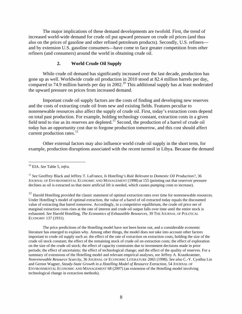
The major implications of these demand developments are twofold. First, the trend of increased world-wide demand for crude oil put upward pressure on crude oil prices (and thus also on the prices of gasoline and other refined petroleum products). Secondly, U.S. refiners—and by extension U.S. gasoline consumers—have come to face greater competition from other refiners (and consumers) around the world in obtaining crude oil.
2. World Crude Oil Supply
While crude oil demand has significantly increased over the last decade, production has gone up as well. Worldwide crude oil production in 2010 stood at 82.4 million barrels per day, compared to 74.9 million barrels per day in 2002.10 This additional supply has at least moderated the upward pressure on prices from increased demand.
Important crude oil supply factors are the costs of finding and developing new reserves and the costs of extracting crude oil from new and existing fields. Features peculiar to nonrenewable resources also affect the supply of crude oil. First, today’s extraction costs depend on total past production. For example, holding technology constant, extraction costs in a given field tend to rise as its reserves are depleted.11 Second, the production of a barrel of crude oil today has an opportunity cost due to forgone production tomorrow, and this cost should affect current production rates.12
Other external factors may also influence world crude oil supply in the short term, for example, production disruptions associated with the recent turmoil in Libya. Because the demand
10 EIA. See Table 5, infra.
11 See Geoffrey Black and Jeffrey T. LaFrance, Is Hotelling’s Rule Relevant to Domestic Oil Production?, 36 JOURNAL OF ENVIRONMENTAL ECONOMIC AND MANAGEMENT (1998) at 155 (pointing out that reservoir pressure declines as oil is extracted so that more artificial lift is needed, which causes pumping costs to increase).
12 Harold Hotelling provided the classic statement of optimal extraction rates over time for nonrenewable resources. Under Hotelling’s model of optimal extraction, the value of a barrel of oil extracted today equals the discounted value of extracting that barrel tomorrow. Accordingly, in a competitive equilibrium, the crude oil price net of marginal extraction costs rises at the rate of interest and crude oil output falls over time until the entire stock is exhausted. See Harold Hotelling, The Economics of Exhaustible Resources, 39 THE JOURNAL OF POLITICAL
ECONOMY 137 (1931).
The price predictions of the Hotelling model have not been borne out, and a considerable economic literature has emerged to explain why. Among other things, the model does not take into account other factors important to crude oil supply such as: the effect of the rate of extraction on extraction costs, holding the size of the crude oil stock constant; the effect of the remaining stock of crude oil on extraction costs; the effect of exploration on the size of the crude oil stock; the effect of capacity constraints due to investment decisions made in prior periods; the effect of uncertainty; the effect of technological change; and the effect of the quality of reserves. For a summary of extensions of the Hotelling model and relevant empirical analyses, see Jeffrey A. Krautkraemer, Nonrenewable Resource Scarcity, 36 JOURNAL OF ECONOMIC LITERATURE 2065 (1998). See also C.-Y. Cynthia Lin and Gernot Wagner, Steady-State Growth in a Hotelling Model of Resource Extraction, 54 JOURNAL OF
ENVIRONMENTAL ECONOMIC AND MANAGEMENT 68 (2007) (an extension of the Hotelling model involving technological change in extraction methods).

9
for crude oil is price inelastic, even relatively small supply disruptions can have significant worldwide price impacts.
Competitive conditions also matter to supply—for crude oil, this issue primarily involves OPEC. We now review competitive conditions in crude oil by updating the industry concentration statistics of the 2004 PETROLEUM MERGER REPORT. OPEC’s role in crude oil prices is discussed next, where we summarize recent learning from the economic literature. A discussion of non-OPEC supply of crude oil and sources of U.S. crude oil imports concludes the section.
a. Industry Concentration in World Crude Oil
The PETROLEUM MERGER REPORT noted that concentration in crude oil may be usefully measured on a current production or a reserves basis. Shares based on current production are better suited to show an entity’s short-run competitive significance, while shares based on reserves are a better long-run indicator. Accordingly, the PETROLEUM MERGER REPORT provided concentration measures on both bases.
The role of foreign governments complicates measurement of crude oil concentration. If a government controls output within its borders then it is a relevant competitive entity for the purposes of calculating shares. But this issue is complex because the extent of government control may vary from country to country. To address this issue we adopt the methodology of the PETROLEUM MERGER REPORT and its predecessors by estimating concentration in two ways. Under the first, the “company approach,” all companies, whether state-owned or private, are assumed to be independent competitors; under the second, the “country approach,” countries are assumed to be the relevant competitive entities, with the exception of the United States and Canada.13
Table 1 shows world concentration in the production of crude oil and associated natural gas liquids (NGLs) under the company approach.14 The Herfindahl-Hirschman Index (HHI) estimate modestly increased from 283 in 2002 to 314 in 2009, but was well below its 1990 level of 527.15 Under the country approach, shown in Table 2, the world crude production HHIs are slightly higher, increasing from 427 in 2002 to 465 in 2009, but were well below the 1990 HHI of 578. Thus, concentration for world crude production has changed little since 2002 and remains unconcentrated.
Concentration estimates based on reserves are shown in Tables 3 (company approach) and Table 4 (country approach). The company-approach reserves HHI increased from 770 in 2002 to 890 in 2009, while country-approach reserves HHI showed a small decline since 2002,
13 For more details on the measurement of crude oil concentration, see PETROLEUM MERGER REPORT, supra note 7, at 131-136.
14 Tables 1 through 15 are located at the end of the report beginning on page 40.
15 The HHI is the sum of squared shares of all industry participants.

10
falling from 812 in that year to 753 in 2009. Both the 2002 and the 2009 country-approach reserves HHIs were below the 1990 level of 1156. In sum, similar to the results based on production, world concentration in crude oil reserves has changed little since 2002 and remains unconcentrated.
As was the case at the time of the PETROLEUM MERGER REPORT, the shares of world production and shares of world reserves of even the largest U.S. petroleum companies have remained very small. For example, in 2009 ExxonMobil’s production and reserve shares of world totals were 3.0% and 0.9% respectively. Corresponding production and reserve shares for ChevronTexaco in 2009 were 2.3% and 0.5% respectively.
Distinguishing between OPEC and non-OPEC controlled production and reserves is important in understanding the supply dynamics of world crude oil, as discussed more fully below. Table 5 shows that OPEC’s share of world crude oil production increased from 39.0% in 2002 to 42.4% in 2010, an increase partly due to membership changes in OPEC. In 2007, Angola joined OPEC, and Ecuador rejoined the organization after having left in 1992. Indonesia left OPEC in 2009 when it ceased being a net exporter of oil.16 Without these membership changes, OPEC’s share of world production would have been 40.6% in 2010. While its production share in 2010 modestly increased from the 2002 level, OPEC’s share of world production was well below its 1974 level of 53.6%.
As can be seen in Table 6, OPEC enjoys a much more commanding position in reserves. OPEC’s share of world crude oil reserves increased from 67.5% in 2002 to 72.1% in 2010. This increase is partially due to changes in OPEC membership, noted above. OPEC’s reserve share would have been 71.3% in 2010 without these membership changes. A part of the increase is attributable to a recent increase in Venezuela’s reported reserves. 17 However, OPEC’s share of reserves in 2010 was less than the 79.2% level reached in 2000.18
b. OPEC
OPEC currently has 12 member countries.19 Its stated mission is “to coordinate and unify the petroleum policies of its Member Countries … in order to secure an efficient, economic and regular supply of petroleum to consumers, a steady income to producers and a fair return on
16 Indonesia to Withdraw from OPEC, BBC NEWS, May 28, 2008, available at http://news.bbc.co.uk/2/hi/7423008.stm.
17 This increase was due to the inclusion of non-conventional extra-heavy crude oil reserves. For more information on this reporting change, see http://www.eia.doe.gov/cabs/venezuela/oil.html (last visited June 1, 2011).
18 The historic peak was in 2001, when OPEC’s share of reserves was 79.4%.
19 OPEC’s current members are Algeria, Angola, Ecuador, Iran, Iraq, Kuwait, Libya, Nigeria, Qatar, Saudi Arabia, United Arab Emirates, and Venezuela. See OPEC: MEMBER COUNTRIES, available at http://www.opec.org/opec_web/en/about_us/25.htm (last visited June 1, 2011).
11
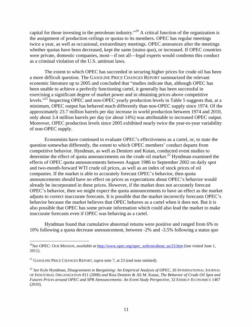
capital for those investing in the petroleum industry.”20 A critical function of the organization is the assignment of production ceilings or quotas to its members. OPEC has regular meetings twice a year, as well as occasional, extraordinary meetings. OPEC announces after the meetings whether quotas have been decreased, kept the same (status quo), or increased. If OPEC countries were private, domestic companies, most—if not all—legal experts would condemn this conduct as a criminal violation of the U.S. antitrust laws.
The extent to which OPEC has succeeded in securing higher prices for crude oil has been a more difficult question. The GASOLINE PRICE CHANGES REPORT summarized the relevant economic literature up to 2005 and concluded that “studies indicate that, although OPEC has been unable to achieve a perfectly functioning cartel, it generally has been successful in exercising a significant degree of market power and in obtaining prices above competitive levels.”21 Inspecting OPEC and non-OPEC yearly production levels in Table 5 suggests that, at a minimum, OPEC output has behaved much differently than non-OPEC supply since 1974. Of the approximately 23.7 million barrels per day increase in world production between 1974 and 2010, only about 3.4 million barrels per day (or about 14%) was attributable to increased OPEC output. Moreover, OPEC production levels since 2005 exhibited nearly twice the year-to-year variability of non-OPEC supply.
Economists have continued to evaluate OPEC’s effectiveness as a cartel, or, to state the question somewhat differently, the extent to which OPEC members’ conduct departs from competitive behavior. Hyndman, as well as Demirer and Kutan, conducted event studies to determine the effect of quota announcements on the crude oil market.22 Hyndman examined the effects of OPEC quota announcements between August 1986 to September 2002 on daily spot and two-month-forward WTI crude oil prices, as well as an index of stock prices of oil companies. If the market is able to accurately forecast OPEC’s behavior, then quota announcements should have no effect on prices as expectations about OPEC’s behavior would already be incorporated in these prices. However, if the market does not accurately forecast OPEC’s behavior, then we might expect the quota announcements to have an effect as the market adjusts to correct inaccurate forecasts. It is possible that the market incorrectly forecasts OPEC’s behavior because the market believes that OPEC behaves as a cartel when it does not. But it is also possible that OPEC has some private information which could also lead the market to make inaccurate forecasts even if OPEC was behaving as a cartel.
Hyndman found that cumulative abnormal returns were positive and ranged from 6% to 10% following a quota decrease announcement, between -2% and -3.5% following a status quo
20See OPEC: OUR MISSION, available at http://www.opec.org/opec_web/en/about_us/23.htm (last visited June 1, 2011).
21 GASOLINE PRICE CHANGES REPORT, supra note 7, at 23 (end note omitted).
22 See Kyle Hyndman, Disagreement in Bargaining: An Empirical Analysis of OPEC, 26 INTERNATIONAL JOURNAL
OF INDUSTRIAL ORGANIZATION 811 (2008) and Riza Demirer & Ali M. Kutan, The Behavior of Crude Oil Spot and Futures Prices around OPEC and SPR Announcements: An Event Study Perspective, 32 ENERGY ECONOMICS 1467 (2010).
12
announcement, and not significantly different from zero following a quota increase announcement.23 Similarly, Demirer and Kutan examined the effect of OPEC quota announcements between March 1983 to June 2008 on daily spot and forward WTI crude oil prices over multiple time horizons. They found that cumulative abnormal returns were positive and ranged from about 4% to nearly 8% following a quota decrease announcement, between -2% and -3% following a status quo announcement, and not significantly different from zero following a quota increase announcement. Thus, both studies found that quota reductions increased crude oil prices, while quota increases had no effect on crude oil prices.
Hyndman suggested that this asymmetric response of the crude oil market to OPEC quota announcements may be because of asymmetric bargaining behavior on the part of OPEC member countries. When prices are increasing, members may come to an agreement more easily on the preferred quota level; therefore a quota increase announcement is expected by the market, and traders have already incorporated this information into the price of oil futures. However, in a period of decreasing prices, it may be more difficult for members to come to an agreement, and thus the market is surprised by both status quo and quota decrease announcements. The market reacts negatively to status quo announcements when a quota decrease announcement was expected. Prices fall because the expectation of higher prices, which had already been incorporated into the current price, was not realized.
Other analysts have considered OPEC’s members’ adherence to assigned quotas. Li found that OPEC members respond to demand and cost shocks differently than non-OPEC members, which presumably behave competitively.24 But Kaufmann et al. demonstrated that OPEC members’ responses to quota changes are typically less than one-to-one.25 That is, a 1% decrease in a member’s quota results in a less than 1% decrease in production. This suggests that OPEC is not fully effective at controlling the production levels of its members.
Bremond et al. found that a subgroup of countries within OPEC—Iran, Libya, Kuwait, Qatar, Saudi Arabia, United Arab Emirates, and Venezuela—coordinate their production decisions, while Hansen and Lindholt found that both Saudi Arabia and the OPEC core countries (Saudi Arabia, Kuwait, Qatar, and United Arab Emirates) exhibit characteristics of a dominant
23 The event study methodology examines price changes in an “event window.” The window includes the date of the announcement as well as several days before and after the announcement. Both of these recent event studies on OPEC quota announcements use windows of about three weeks. The daily changes in oil and stock prices outside the window are referred to as normal returns. The differences between the daily price changes in the window and the daily price changes outside the window are referred to as abnormal returns. Cumulative abnormal returns are the sum of the abnormal returns resulting from the quota announcement.
24 See Raymond Li, The Role of OPEC in the World Oil Market, 9(1) INTERNATIONAL JOURNAL OF BUSINESS &
ECONOMICS 83 (2010). Formally, Li finds that OPEC output is not cointegrated with non-OPEC output.
25 See Robert K. Kaufmann, Andrew Bradford, Laura H. Belanger, John P. Mclaughlin, &Yosuke Miki, Determinants of OPEC Production: Implications for OPEC Behavior, 30 ENERGY ECONOMICS 333 (2008).

13
firm.26 Dominant firms choose their production level by equating marginal revenue to marginal cost while taking the production levels of fringe firms as given. As a consequence, dominant firms generally produce less output relative to competitive price takers.27
While OPEC has some cartel characteristics, some analysts see it behaving more like a price-taking, competitive firm. Smith noted that, “[s]ince the quota system was adopted in 1983, total OPEC production has exceeded the agreed ceiling by 4% on average, but on numerous occasions the excess has run to 15% or more.”28 Kaufmann et al. found that OPEC production is not inversely related to changes in the crude oil price and see some evidence that OPEC production may respond positively to increases in the crude oil price. This type of response is consistent with price-taking.
In addition, Bremond et al. found that OPEC as a whole exhibits price-taking behavior. This finding is reinforced by Dibooglu and AlGudhea (2007), who found that changes in the crude oil price cause OPEC members to cheat on their assigned quotas.29 But cheating responds asymmetrically to price changes with several OPEC members cheating more in response to negative price changes than positive price changes. Furthermore, Dibooglu and AlGudhea concluded that Saudi Arabia does not accommodate cheating by other members by reducing its production, and Saudi Arabia only punishes cheating with production increases if the cheating is especially large.
While OPEC may not be fully successful in constraining current production, its members may have had more success in constraining investments in new production capacity. OPEC’s 2010 production capacity of 33.7 million barrels per day is roughly equivalent to its actual production in 1974 despite a doubling of its proved reserves since that time.30 Smith notes that, “in 2007, the super-majors [the five largest international oil companies] reinvested 25% of their gross production revenues to expand [production] capacity, whereas OPEC members are investing only about 6% of their net export revenues on such projects.”31 While there is a joint interest in limiting production capacity investment, OPEC members claim to make their
26 See Vincent Bremond, Emmanuel Hache, & Valerie Mignon, Does OPEC Still Exist as a Cartel? An Empirical Investigation, forthcoming, ENERGY ECONOMICS (2011) and Petter Vegard Hansen & Lars Lindholt, The Market Power of OPEC 1973-2001, 40 APPLIED ECONOMICS 2939 (2008).
27 If the sub-group of OPEC countries from Bremond et al. is treated as a single entity, the 2009 production HHI reported in Table 2 increases to 1142 and the 2009 reserves HHI reported in Table 4 increases to 3295. If, instead, the sub-group of OPEC countries from Hansen and Lindholt is treated as a single entity, then the 2009 production HHI increases to 672 and the 2009 reserves HHI increases to 1550.
28 See Smith, supra note 9, at 152.
29 See Sel Dibooglu & Salim N. AlGudhea, All Time Cheaters versus Cheaters in Distress: An Examination of Cheating and Oil Prices in OPEC, 31 ECONOMIC SYSTEMS 292 (2007).
30 See EIA, SHORT TERM ENERGY OUTLOOK, May 10, 2011, at Table 3c, available at http://www.eia.doe.gov/steo/3ctab.pdf, and also Table 5 and Table 6, infra.
31 Smith, supra note 9, at 153 (emphasis in original).

14
investment decisions independently.32 To the extent that OPEC members have success in constraining investment in production capacity beyond what might occur in an efficient, competitive marketplace, crude oil prices might be expected to be higher than they otherwise would have been. However, sovereign nations may have different incentives to invest than private firms. This could be due to different discounts rates.33
In sum, the recent economic literature suggests that OPEC clearly has some ability to influence the crude oil price, as suggested by the crude oil market’s response to some of its quota announcements. OPEC, or at least some subset of its important members, has some characteristics of a cartel, but members’ cheating on the assigned quotas has limited its effectiveness as a cartel. However, OPEC members may have had more success in limiting investments in new production capacity.
c. Non-OPEC Supply
The supply responsiveness of non-OPEC producers limits whatever ability OPEC does have in exercising market power.34 While OPEC production has increased by about 0.5% since 2005, non-OPEC output has increased by about 1.9%.35 It is likely that without higher prices, non-OPEC output would not have increased as much, and one analyst in 2009 estimated that it would be falling.36 Expectations of declining non-OPEC supply are based on the fact that many
32 See Press Release, OPEC, OPEC 157TH Meeting Concludes, October 14, 2010, available at http://www.opec.org/opec_web/en/press_room/1906.htm and Keynote Address, HE Abdalla S. El-Badri, Reflecting on Oil Investment, available at http://www.opec.org/opec_web/en/press_room/1986.htm, January 31, 2011.
33 See El-Badri, supra note 32 (discusses leaving resources in the ground for future generations).
34 Most analysts would characterize non-OPEC suppliers as price takers. In the past, however, some large, non-OPEC oil producing countries may have coordinated output decisions with OPEC. See PETROLEUM MERGER
REPORT, supra note 7, at 138. In late 2008, OPEC reportedly solicited Russia, Norway, and Mexico to join it in reducing output as crude oil prices fell during the global recession. See, e.g., Andres R. Martinez, Mexico Says Moves to Stabilize Oil Market ‘Positive’, BLOOMBERG NEWS, December 16, 2008, available at http://www.bloomberg.com/apps/news?pid=newsarchive&sid=aSt_oQJvLdCs&refer=news. None of these countries agreed to cut output according to later reports. See Katya Glubkova and Gleb Gorodyankin, WRAPUP 2-Azerbaijan, not Russia, Offers OPEC Oil Cut, REUTERS, December 17, 2008, available at http://uk.reuters.com/article/2008/12/17/opec-nonopec-idUKLH50973720081217.
35 EIA, International Energy Statistics, Annual Petroleum Production, Production of Crude Oil Including Lease Condensate, 2005 to 2010, http://www.eia.gov/cfapps/ipdbproject/iedindex3.cfm?tid=5&pid=57&aid=1&cid=all,&syid=2005&eyid=2010&unit=TBPD; EIA, International Energy Statistics, Annual Petroleum Production, Production of Natural Gas Plant Liquids, 2005 to 2010, http://www.eia.gov/cfapps/ipdbproject/iedindex3.cfm?tid=5&pid=58&aid=1&cid=all,&syid=2005&eyid=2010&unit=TBPD. These production amounts are based on current production of current OPEC members for both 2005 and 2010, subtracting Indonesia’s production from 2010, and adding Ecuador and Angola’s production from 2005.
36 See Smith, supra note 9, at 151, 159.

15
large oil fields in non-OPEC countries have peaked and have seen falling production, and that replacing these depleted fields is increasingly expensive.37
Based on Energy Information Administration (EIA) data and taking into account membership changes, non-OPEC production increased from 46.6 million barrels per day to 47.5 million barrels per day between 2005 and 2010.38 The largest increases were in the United States, Russia, and Azerbaijan. Each of these countries increased production by around 0.6 million barrels per day. Some of the increase for the United States was due to lost production in 2005 after the Gulf hurricanes coming back online, but production was up almost 0.3 million barrels per day since 2004. Other non-OPEC countries that increased production significantly were China (almost 0.5 million barrels per day), Brazil (over 0.4 million barrels per day), and Canada (almost 0.4 million barrels per day). There also was a significant increase in biofuels production, up from 0.1 million barrels per day to 1.8 million barrels per day.39
Canada, now the largest supplier of crude oil imports to the United States, increased its output significantly over the last decade. The main factor in this growth has been the development of its oil sands reserves, exploitation of which requires non-conventional oil extraction processes that have become economically viable as crude oil prices increased and extraction technology has improved. Canadian conventional oil production, on the other hand, decreased 12% between 2001 and 2010. However, overall Canadian crude oil production increased 41% due to the 167% increase in non-conventional crude production.40
In the United States, as oil prices have increased, so have the number of development rigs.41 After reaching a recent low of around 6.7 million barrels per day several times between 2006 and 2008 (not including significant monthly decreases due to Gulf hurricanes), domestic crude oil and NGL production increased to 7.7 million barrels per day by the end of 2010.42 Most of the growth in U.S. production came from the Gulf of Mexico, North Dakota, and Texas, with smaller increases in other areas. Overall, these increases more than offset the decreased production in Alaska’s North Slope and in other areas such as California and Montana.
37 For example, production in Mexico, Norway, and the United Kingdom have fallen significantly over the last five years.
38 EIA, supra note 26.
39 International Energy Agency (IEA) OIL MARKET REPORT, various issues, available at http://omrpublic.iea.org/.
40 National Energy Board, Estimated Production of Canadian Crude Oil and Equivalent, available at http://www.neb-one.gc.ca/clf-nsi/rnrgynfmtn/sttstc/crdlndptrlmprdct/stmtdprdctn-eng.html.
41 See Smith, supra note 9, at 160.
42 EIA, supra note 26.
16
d. Crude Supply to U.S. Refineries
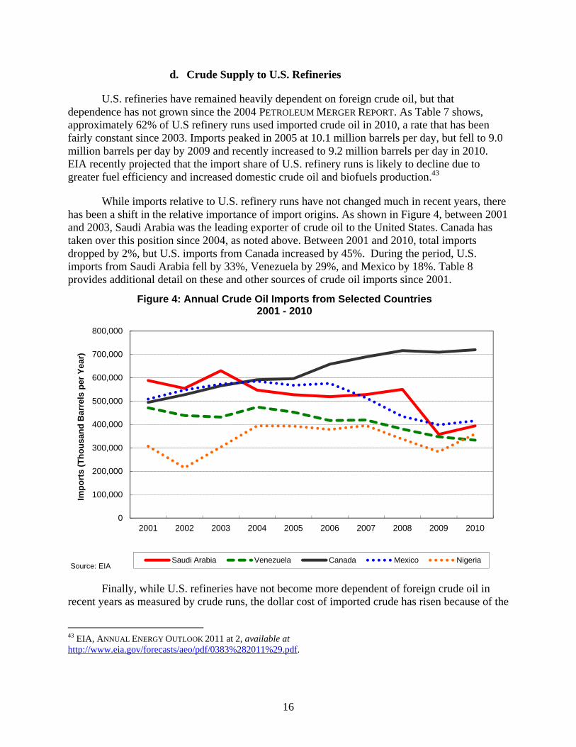
U.S. refineries have remained heavily dependent on foreign crude oil, but that dependence has not grown since the 2004 PETROLEUM MERGER REPORT. As Table 7 shows, approximately 62% of U.S refinery runs used imported crude oil in 2010, a rate that has been fairly constant since 2003. Imports peaked in 2005 at 10.1 million barrels per day, but fell to 9.0 million barrels per day by 2009 and recently increased to 9.2 million barrels per day in 2010. EIA recently projected that the import share of U.S. refinery runs is likely to decline due to greater fuel efficiency and increased domestic crude oil and biofuels production.43
While imports relative to U.S. refinery runs have not changed much in recent years, there has been a shift in the relative importance of import origins. As shown in Figure 4, between 2001 and 2003, Saudi Arabia was the leading exporter of crude oil to the United States. Canada has taken over this position since 2004, as noted above. Between 2001 and 2010, total imports dropped by 2%, but U.S. imports from Canada increased by 45%. During the period, U.S. imports from Saudi Arabia fell by 33%, Venezuela by 29%, and Mexico by 18%. Table 8 provides additional detail on these and other sources of crude oil imports since 2001.
Finally, while U.S. refineries have not become more dependent of foreign crude oil in recent years as measured by crude runs, the dollar cost of imported crude has risen because of the
43 EIA, ANNUAL ENERGY OUTLOOK 2011 at 2, available at http://www.eia.gov/forecasts/aeo/pdf/0383%282011%29.pdf.
0
100,000
200,000
300,000
400,000
500,000
600,000
700,000
800,000
2001 2002 2003 2004 2005 2006 2007 2008 2009 2010
Imp
ort
s (T
ho
usa
nd
Bar
rels
per
Yea
r)
Figure 4: Annual Crude Oil Imports from Selected Countries 2001 - 2010
Saudi Arabia Venezuela Canada Mexico NigeriaSource: EIA
17
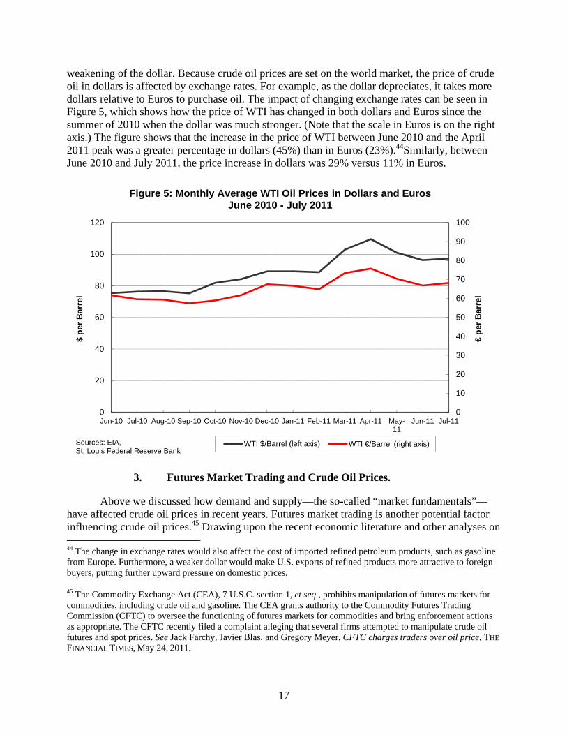
weakening of the dollar. Because crude oil prices are set on the world market, the price of crude oil in dollars is affected by exchange rates. For example, as the dollar depreciates, it takes more dollars relative to Euros to purchase oil. The impact of changing exchange rates can be seen in Figure 5, which shows how the price of WTI has changed in both dollars and Euros since the summer of 2010 when the dollar was much stronger. (Note that the scale in Euros is on the right axis.) The figure shows that the increase in the price of WTI between June 2010 and the April 2011 peak was a greater percentage in dollars (45%) than in Euros (23%).44Similarly, between June 2010 and July 2011, the price increase in dollars was 29% versus 11% in Euros.
3. Futures Market Trading and Crude Oil Prices.
Above we discussed how demand and supply—the so-called “market fundamentals”—have affected crude oil prices in recent years. Futures market trading is another potential factor influencing crude oil prices.45 Drawing upon the recent economic literature and other analyses on 44 The change in exchange rates would also affect the cost of imported refined petroleum products, such as gasoline from Europe. Furthermore, a weaker dollar would make U.S. exports of refined products more attractive to foreign buyers, putting further upward pressure on domestic prices.
45 The Commodity Exchange Act (CEA), 7 U.S.C. section 1, et seq., prohibits manipulation of futures markets for commodities, including crude oil and gasoline. The CEA grants authority to the Commodity Futures Trading Commission (CFTC) to oversee the functioning of futures markets for commodities and bring enforcement actions as appropriate. The CFTC recently filed a complaint alleging that several firms attempted to manipulate crude oil futures and spot prices. See Jack Farchy, Javier Blas, and Gregory Meyer, CFTC charges traders over oil price, THE
FINANCIAL TIMES, May 24, 2011.
0
10
20
30
40
50
60
70
80
90
100
0
20
40
60
80
100
120
Jun-10 Jul-10 Aug-10 Sep-10 Oct-10 Nov-10 Dec-10 Jan-11 Feb-11 Mar-11 Apr-11 May-11
Jun-11 Jul-11
€p
er B
arre
l
$ p
er B
arre
l
Figure 5: Monthly Average WTI Oil Prices in Dollars and Euros June 2010 - July 2011
WTI $/Barrel (left axis) WTI €/Barrel (right axis)Sources: EIA, St. Louis Federal Reserve Bank

18
the topic, here we examine the connection between futures trading and the spot prices for physical barrels of crude oil.46 We begin with a discussion of the institutional background.
As the PETROLEUM MERGER REPORT showed, the growth of crude oil futures trading and the accompanying expansion of spot market trading are relatively recent phenomena (compared to such trading in agricultural commodities), dating back to the late 1970s. As the PETROLEUM
MERGER REPORT concluded, the expansion of futures and spot trading may have reduced the incentives for vertical integration between petroleum industry’s upstream (crude oil) and downstream (refining and marketing) levels. Moreover, the expansion of futures and spot trading appeared to have provided for more efficient allocation of price risks among producers, refiners, and other traders, and also facilitated contracting between buyers and sellers to allow future price terms to be set in reference to widely recognized spot or futures prices.47
As to price risks in particular, crude oil prices can display significant volatility.48 Because crude oil supply and demand are very inelastic in the short run—i.e., insensitive to price changes—small changes to either can produce large swings in spot prices. Price volatility poses a problem for producers and consumers of crude oil who must make long-term planning decisions. Traditional futures contracts—including the New York Mercantile Exchange (NYMEX) contract for WTI crude—reduce the uncertainty posed by volatile spot prices by allowing buyers and sellers to lock in a specific price for oil delivery at some point in the future.49 NYMEX contracts are available for many different delivery dates, ranging from two months distant to over eight
While it has neither the CFTC’s direct expertise nor that agency’s statutory responsibilities regarding
futures markets, the FTC, as part of its interests in enforcing the antitrust laws and maintaining competition, has examined whether control of certain physical assets might be used to affect futures prices. See BP Amoco p.l.c. FTC Dkt. No C-3938 (Analysis of the Proposed Consent Order and Draft Complaint to Aid Public Comment), available at http://www.ftc.gov/os/2000/04/bpamoco.htm (allegation that acquisition of ARCO would enhance BP’s ability to manipulate crude oil futures prices). See also KATRINA REPORT, infra note 58, at 53-56 (examination of whether gasoline futures prices might be manipulated through control of storage in the New York Harbor area). Furthermore, the FTC in 2009 issued a Market Manipulation Rule, which prohibits market manipulation in wholesale petroleum products through fraudulent or deceptive acts, practices or courses of business. See FTC Market Manipulation Rule Webpage, available at http://www.ftc.gov/ftc/oilgas/rules.htm. Recognizing the connections between their areas of enforcement responsibilities, the CFTC and FTC recently signed a Memorandum of Understanding to facilitate sharing of non-public information on investigations conducted by the agencies. See Press Release, FTC, FTC, CFTC Agree to Share Information on Energy Investigations, April 12, 2011, available at http://www.ftc.gov/opa/2011/04/ftccftc-mou.shtm.
46 Spot prices involve bulk sales of crude oil and other petroleum products for immediate delivery, not subject to a longer term contract. Futures and spot trading in gasoline and other refined products also occurs, and it raises the same issues as in crude oil regarding possible price effects in the corresponding physical markets.
47 PETROLEUM MERGER REPORT, supra note 7, at 140-1.
48 Eva Regnier, Oil and energy price volatility, 29 ENERGY ECONOMICS 405 (2007).
49 Other futures contracts—including the Intercontinental Exchange (ICE) contract for WTI crude—serve the same purpose but are settled for cash.

19
years in the future.50 In general, there is an inverse relationship between the contract’s trading volume and the time until delivery.51
Participants in commodities futures markets are often divided into two types: commercial participants whose business operations directly expose them to the price volatility of the physical commodities, and financial participants who trade in futures exchanges because commodity prices have historically had desirable investment properties, such as low or negative correlations with other asset classes.52 Commercial participants, who are often called “hedgers,” use futures markets to hedge their exposure to risk by taking offsetting positions in the market. For example, an oil refiner mitigates the risk of an increase in the crude oil price by locking in its future price. On the other side of the transaction, a crude oil producer might be hedging its exposure to the risk of a price decline. Purely financial participants in futures markets do not have fundamental exposure to petroleum-based business risks. Because of this, they have often been referred to as “speculators” to distinguish them from the commercial traders engaging in hedging behavior. Despite the negative connotations to this term, the presence of financial traders in futures markets has traditionally been seen as beneficial, as they provide necessary liquidity to the market, helping to ensure that hedgers can efficiently mitigate their risks.53
By allowing commercial firms to hedge business risks and financial traders to diversify their portfolios, futures markets can serve as a means of aggregating and distributing valuable market information.54 For example, if some futures market participants believe—perhaps as a result of private information—that the future price of a commodity will be higher, they can take a long position in the futures market. When a significant number of participants take such positions, the price for delivery at that date rises in the futures market, and this price increase will likely affect contemporaneous behavior and the spot price. If the futures price is much higher than the spot price, participants in the spot market have an incentive to change their behavior. Producers should reduce their current production or increase their inventories, because it will be more profitable to deliver later. Similarly, buyers should begin to stockpile oil before the price increases. Both of these impulses lead the spot price to rise to a new equilibrium that
50 Details on NYMEX contracts are available at http://www.cmegroup.com/trading/energy/crude-oil/light-sweet-crude_contract_specifications.html (last visited June 1, 2011).
51 Contracts for delivery at the end of calendar years are disproportionately popular.
52 IMF, GLOBAL FINANCIAL STABILITY REPORT: FINANCIAL STRESS AND DELEVERAGING, MACRO-FINANCIAL
IMPLICATIONS AND POLICY (October 2008), available at http://www.imf.org/external/pubs/ft/gfsr/2008/02/index.htm. See also Presentation by Richard Newell, Energy and Financial Markets Overview: Crude Oil Price Formation, at 26, available at http://www.eia.gov/neic/speeches/newell_02232011.pdf.
53 David S. Jacks, Populists versus theorists: Futures markets and the volatility of prices, 44 EXPLORATIONS IN
ECONOMIC HISTORY 342 (2007).
54 Sanford J. Grossman, The Existence of Futures Markets, Noisy Rational Expectations and Informational Externalities, 44(3) THE REVIEW OF ECONOMIC STUDIES 431 (1977).

20
redistributes consumption to later time periods. This redistribution is efficient if the futures market correctly predicts future supply and demand conditions.
This connection between futures and spot markets—and specifically the role of speculators in futures markets—has led to a suspicion that futures market activity may cause spot prices to change, independent of any changes in spot market fundamentals, such as output reductions or increased inventory holdings.55 Several factors have magnified concerns about speculative effects in recent years. Many commodities’ prices—prominently including crude oil–have increased dramatically in relatively short periods of time. For example, the price of crude oil rose from $34 per barrel in January 2004 to a peak at $145 per barrel on July 3, 2008. Similar increases, though less dramatic, have occurred more recently. At the same time it has been reported that the volume of futures trading for crude oil and other commodities has also risen dramatically. The International Monetary Fund (IMF) reports that investment in commodity-related assets increased from less than $10 billion to $230 billion between 1997 and 2008.56 Finally, it has been noted that greater participation by non-commercial financial traders has accounted for much of this increase. A recent study documents that the volume of crude oil futures trading accounted for by financial firms more than doubled to exceed 40% of all open futures and futures-equivalent option positions during roughly this same period.57
This observed correlation between the increase in commodity prices and rising financial trader participation in futures markets has led concerned parties to focus on two possible mechanisms that could lead to purely speculative effects on spot prices. First, it has been suggested that the dramatically increased participation by non-commercial traders taking long positions represents a demand shock that causes spot prices to increase.58 Second, it is argued that if investment in futures markets is more affected by herd-behavior or irrational expectations, it could lead to speculative bubbles (or craters) or to greater spot price volatility.59
The dramatic increase in participation (especially speculative participation) in commodities future markets has led to increased scrutiny of crude oil—as well as other commodity—markets by government agencies, intergovernmental organizations, and academic researchers.60,61 While all of these studies generally analyze the extent to which activities in 55 Jacks, supra note 53.
56 IMF, THE WORLD ECONOMIC OUTLOOK (October 2008), at 88, available at http://www.imf.org/external/pubs/ft/weo/2008/02/.
57 Bahattin Buyuksahin, Michael S. Haigh, Jeffrey H. Harris, James A. Overdahl, and Michel A. Robe, Fundamentals, Trader Activity and Derivative Pricing (December 4, 2008), available at http://www.cftc.gov/ucm/groups/public/@newsroom/documents/file/marketreportenergyfutures.pdf.
58 Smith, supra note 9.
59 J. Bradford de Long, Andrei Shleifer, Lawrence H. Summers, and Robert J. Waldmann, Positive Feedback Investment Strategies and Destabilizing Rational Speculation, 45(3) THE JOURNAL OF FINANCE 379 (1990).
60 Michael W. Masters, Testimony before the Committee on Homeland Security and Government Affairs, U.S. Senate (May 20, 2008), available at http://hsgac.senate.gov/public/_files/052008Masters.pdf; see also various statements quoted in Committee on Homeland Security and Governmental Affairs, U.S. Senate, The Role of Market

21
futures markets have a systematic influence on spot prices, some focus on the level of spot price effects and others on the volatility of spot prices.
At present, however, there is little consensus in the resulting literature.62 On the one hand, some analysts conclude that increased non-commercial participation in futures markets clearly has affected spot market prices.63 Other papers argue that the higher volume of trading in the futures market represents a speculative bubble, and that this bubble was then transmitted to spot markets.64 Other papers argue that volatility shocks in the futures market affect the volatility of spot prices without making the argument that the changes produced a speculative bubble.65 Finally, a number of reports find evidence both that futures market prices can impact spot markets, but also that spot market prices can impact futures markets.66
On the other hand, at least as many reports conclude that futures markets do not have a systematic influence on spot prices for crude oil or other commodities as those reports that conclude the opposite. For example, an IMF study examines the futures positions of non-commercial traders in connection with and spot prices for a number of different commodities, including crude oil. Based on a series of statistical tests, the study concludes that almost none of
Speculation in Rising Oil and Gas Prices: A Need to Put the Cop Back on the Beat (June 27, 2006), available at http://hsgac.senate.gov/public/_files/SenatePrint10965MarketSpecReportFINAL.pdf.
61 A large number of these studies are reviewed and summarized in Scott H. Irwin and Dwight R. Sanders, Index Funds, Financialization, and Commodity Futures Markets, 33(1) APPLIED ECONOMIC PERSPECTIVES AND POLICY 1 (2011).
62 A similar review by another Federal agency has reached the same conclusion. See Presentation by Richard Newell, supra note 52.
63 Committee on Homeland Security and Governmental Affairs, U.S. Senate (2006), supra note 60; Kenneth B. Medlock III and Amy Myers Jaffe, Who is in the Oil Futures Market and How Has it Changed? (August 2009), available at http://www.bakerinstitute.org/publications/EF-pub-MedlockJaffeOilFuturesMarket-082609.pdf; Lonnie K. Stevans and David N. Sessions, Speculation, Futures Prices, and the US Real Price of Crude Oil, 1 AMERICAN
JOURNAL OF SOCIAL AND MANAGEMENT SCIENCES 13 (2010); Robert K. Kaufmann and Ben Ullman, Oil Prices, Speculation, and Fundamentals: Interpreting Causal Relations Among Spot and Futures Prices, 31 ENERGY
ECONOMICS 550 (2009).
64 Christopher L. Gilbert, Speculative Influences on Commodity Futures Prices 2006-08 (October 2009), available at http://www.nottingham.ac.uk/economics/documents/seminars/senior/christopher-gilbert-04-11-09.pdf; Peter C. B. Phillips and Jun Yu, Dating the Timeline of Financial Bubbles During the Subprime Crisis (2010), available at http://cowles.econ.yale.edu/P/cd/d17b/d1770.pdf.
65 Nikos K. Nomikos and Panos K. Pouliasis, Forecasting Petroleum Futures Markets Volatility: The Role of Regimes and Market Conditions, 31 ENERGY ECONOMICS 321 (2011); Xiaodong Du, Cindy L. Yu, and Dermot J. Hayes, Speculation and Volatility Spillover in the Crude Oil and Agricultural Commodity Markets: A Bayesian Analysis, 33 ENERGY ECONOMICS 497 (2011).
66 Stelios D. Bekiros and Cees G.H. Diks, The Relationship between crude oil spot and futures prices: Cointegration, linear and nonlinear causality, 30 ENERGY ECONOMICS 2673 (2008); Bwo-Nung Huang, C.W. Yang, and M.J. Hwang, The dynamics of a nonlinear relationship between crude oil spot and futures prices: A multivariate threshold regression approach, 31 ENERGY ECONOMICS 91 (2009).

22
the markets exhibit signs that the futures prices systematically cause variation in spot markets.67 A number of studies by both research organizations and academics argue that the futures markets are not responsible for changes to spot price levels.68 Many of these studies proceed on the basis that higher futures prices would induce firms to increase inventories which would then affect spot prices, but they conclude that the data do not support this. There is also evidence that futures investment positions by commodity index funds moved counter to spot prices during 2008-2009, which would indicate that the spot price increases during this time were not caused by an increase in positions by these index funds.69 Similarly, at times when spot prices experienced very significant increases, they often remained higher than futures prices—i.e., in backwardation. This again is inconsistent with some theories linking futures prices to higher spot prices.70 There are also a number of studies examining the linkage between financial firm involvement in futures markets and spot price volatility rather than the level of prices. These studies have not found that activity in futures markets increases spot price volatility.71
The literature’s ambiguity in establishing the presence (or absence) of a link between speculative trading and spot prices that is not grounded in market fundamentals is not surprising. First, locating data that distinguish between speculation and hedging is difficult. Many studies rely on CFTC data that distinguish between commercial and non-commercial traders. However, the difference between hedging and speculation does not perfectly conform to the difference
67 IMF, supra note 52.
68 Technical Committee of the International Organization of Securities Commissions, Task Force on Commodity Futures Markets (March 2009), available at https://www.iosco.org/library/pubdocs/pdf/IOSCOPD285.pdf; Noel Amenc, Benoit Maffei, and Hilary Till, Oil Prices: The True Role of Speculation (November 2008), available at http://www.edhec-risk.com/features/RISKArticle.2008-11-26.0035/attachments/EDHEC%20Position%20Paper%20Oil%20Prices%20and%20Speculation.pdf; Craig Pirrong, No Theory? No Evidence? No Problem!, 33 REGULATION 38 (2010); Scott H. Irwin, Dwight R. Sanders, and Robert P. Merrin, Devil or Angel? The Role Speculation in the Commodity Price Boom (and Bust), 41(2) JOURNAL OF
AGRICULTURAL AND APPLIED ECONOMICS 377 (2009); George M. Korniotis, Does Speculation Affect Spot Price Levels? The Case of Metals with and without Futures Markets (2009), available at http://www.federalreserve.gov/pubs/feds/2009/200929/200929pap.pdf; Lutz Kilian and Daniel P. Murphy, The Role of Inventories and Speculative Trading in the Global Market for Crude Oil (May 2010), available at http://www-personal.umich.edu/~lkilian/km031610.pdf; James D. Hamilton, Understanding Crude Oil Prices, 30(2) ENERGY
JOURNAL 179 (2009); Smith, supra note 9.
69 See Presentation by Richard Newell, supra note 52 at 34.
70 See Hamilton, supra note 68, Figure 3. Backwardation does not necessarily imply that a change to futures prices could not increase spot prices. The presence of a convenience yield or a response to risk could explain backwardation. See, e.g., Robert H. Litzenberger and Nir Rabinowitz, Backwardation in Oil Futures Markets: Theory and Empirical Evidence, 50(5) THE JOURNAL OF FINANCE 1517 (1995). These issues might also explain why scholars have not found futures prices to be better predictors of future spot prices than contemporaneous spot prices. See Hamilton, supra note 68, at 185.
71 IMF, supra note 56,at 91; Nicole M. Aulerich, Scott H. Irwin, and Philip Garcia, The Price Impact of Index Funds in Commodity Futures Markets: Evidence from the CFTC’s Daily Large Trader Reporting System (unpublished manuscript) (January 2010), available at http://farmdoc.illinois.edu/irwin/research/PriceeImpactIndexFund,%20Jan%202010.pdf; Jacks, supra note 53.

23
between commercial and non-commercial traders. In some cases, commodity consumers effectively engage in speculation by selecting the degree to which they hedge their exposure to the price of the commodity they consume. Conversely, financial firms often are passive participants in futures markets, assembling portfolios that give their investors exposure to a broad array of asset classes.72
Second, there is little question that recent dramatic increases in spot prices have been coincident with equally dramatic increases in speculative activity in futures markets. However, correlation does not necessarily imply causation, and reasoned explanations of the mechanism by which activity in the futures market affects prices in the physical market have been missing or incomplete in many of the studies. Moreover, many of the studies have relied on statistical causality tests to establish the existence or absence of a consistent relationship between futures market activity and spot market prices. While these tests are well-established in the economic literature, they often require strong assumptions, which are not always tested. This is particularly true of those studies making use of statistical, “Granger causality” tests, which in the absence of particularly strong assumptions do not establish causality in the sense that researchers and policymakers generally understand the term.73
Third, many studies have pursued the narrow goal of establishing whether or not data support the existence of a systematic relationship between futures and spot markets. This ignores the deeper question of whether or not finding evidence of such a linkage would be concerning. As noted above, one of the chief virtues associated with futures markets is their ability to collect and disseminate information. In this case, variation in spot prices in the wake of changes to futures prices may be efficient, as it signals changing expectations about the future value of commodities. Thus, there is a need not only to establish a connection between futures and spot prices, but also to show that the connection is inefficient. It would be particularly difficult for a researcher to first determine the efficient connection between these markets, and then to identify whether the current outcome is significantly different from the efficient outcome.
C. Other Factors Associated with Gasoline Price Changes
Figure 6 shows the components of national average gasoline prices (including taxes) between January 2000 and June 2011 that were attributable to crude oil costs, gross refinery margins, gross distribution/marketing margins, and taxes. Crude oil costs were the largest—and most volatile—component of gasoline prices since 2005. State, Federal, and local taxes, on the other hand, were a very stable component.
Gross refinery margins and gross distribution/marketing margins have shown some volatility since 2005, but their volatility was smaller than that for crude oil costs. The most significant increases in refinery margins occurred during the summers of 2005, 2006, and 2007.
72 Smith, supra note 9.
73 Thomas F. Cooley and Stephen F. LeRoy, Atheoretical Macroeconometrics: A Critique, 16 JOURNAL OF
MONETARY ECONOMICS 283 (1985); Edward E. Leamer, Vector Autoregressions for Causal Inference?, 22 CARNEGIE-ROCHESTER CONFERENCE SERIES ON PUBLIC POLICY 255 (1985).

24
We discuss these episodes next. Between the end of 2007 and March 2011, refinery margins generally returned to their historical norms. A noticeable increase in distribution/marketing margins occurred in late 2008, when crude and gasoline prices fell sharply. The accompanying increase in distribution/marketing margins at this time appeared to be largely due to lagged price adjustments along the petroleum products supply chain, a topic which we treat more fully in Section III.
1. The 2005 Hurricanes
Hurricane Katrina, which made landfall on August 29, 2005, caused the immediate loss of 27% of the nation’s crude oil production and 13% of national refining capacity.74 Shipping on many of the product and crude pipelines leaving the Gulf Coast was also disrupted. As a result, gasoline prices increased significantly throughout the United States. The price increases were higher east of the Rockies, and the largest increases were on the East Coast. Prices were falling back towards pre-Katrina levels when Hurricane Rita made landfall on September 23 and caused the loss of another 8% of crude production and 14% of refining capacity. By four weeks after Hurricane Rita, prices in many areas had returned to pre-Katrina levels, and by December, prices
74 For more details, see FTC, REPORT ON THE FTC'S INVESTIGATION OF GASOLINE PRICE MANIPULATION AND POST-KATRINA PRICE INCREASES [hereinafter KATRINA REPORT] (2006), available at http://www.ftc.gov/reports/060518PublicGasolinePricesInvestigationReportFinal.pdf.
$0.00
$0.50
$1.00
$1.50
$2.00
$2.50
$3.00
$3.50
$4.00
$4.50
Jan-00 Jan-01 Jan-02 Jan-03 Jan-04 Jan-05 Jan-06 Jan-07 Jan-08 Jan-09 Jan-10 Jan-11
Pri
ce (
Do
llars
per
Gal
lon
)Figure 6: Components of Nominal Monthly
Retail Gasoline Prices January 2000 - June 2011
Crude OilRefiningDistribution & MarketingTaxes
Source: EIA

25
had returned to where they were early in the summer of 2005. While the price increases following the hurricanes were significant, the price spike was relatively short-lived.
The hurricane price spike provided incentives for unaffected refiners to increase utilization and for firms to import gasoline from overseas to help reduce the shortage. Capacity utilization at Gulf refineries that were not damaged increased significantly. Gasoline production in the Midwest and on the East Coast also increased. Gasoline imports increased by late September, and for the first two weeks of October, imports were at record levels, about 40% higher than the average level for that time of year.
2. The 2006 and 2007 Summer Price Spikes
Several factors combined to lead to high gasoline prices relative to crude oil in the spring and summer of 2006.75 These included the seasonal effects of the summer driving season, increases in the price of crude oil, increases in the price of ethanol, capacity reductions due to the transition from methyl tertiary butyl ether (MTBE) to ethanol, refinery outages, including lingering effects from the 2005 hurricanes, and an increase in consumer demand for gasoline.
Gasoline formulations are changed to meet regulations to reduce evaporation during the summer. As a result, refiners must decrease the use of relatively volatile gasoline components in the summer, effectively reducing refineries’ gasoline production capacity. This effective capacity reduction, combined with the increase in demand for gasoline during the summer driving season, often leads to higher summer gasoline prices. Moreover, in Summer 2006, almost all reformulated gasoline (RFG) sold in the United States was blended with ethanol, while in the past MTBE was also used to make RFG. 76 In 2005, 12.7% of overall gasoline production was RFG blended with MTBE. Because gasoline blended with ethanol is more volatile than similar gasoline blended with MTBE, this change required refiners to remove even more volatile components in Summer 2006. As a result, effective capacity was reduced much more than in previous summers. The rapid changeover from MTBE to ethanol also led to a shortage of ethanol, causing ethanol prices to increase from around $2.50 per gallon to a peak over $4.00 per gallon. Once the summer driving season was over and the more stringent gasoline specifications were no longer required, gasoline prices returned to a more normal relationship with crude prices.
Factors responsible for the high prices of Summer 2006 were to some extent still present in Summer 2007. The impact of the summer driving season in increasing demand was again evident, and even though average prices were higher in Summer 2007, gasoline consumption increased relative to 2006. The required summer formulations again reduced effective refining
75 For more details, see FTC, REPORT ON SPRING/SUMMER 2006 NATIONWIDE GASOLINE PRICE INCREASES (2007), available at http://www.ftc.gov/reports/gasprices06/P040101Gas06increase.pdf.
76 RFG is formulated to reduce pollution relative to conventional gasoline and is used in “non-attainment areas” to meet Clear Air Act requirements.

26
capacity, although ethanol prices had fallen by then. Furthermore, there were unplanned refinery down-time in Summer 2007.77
By Summer 2008, overall demand had begun to fall due to the recession. This was the first decrease in gasoline consumption relative to the prior summer since 1992. Along with the decrease in demand, there was also an increase in refineries’ upgrading capacity, allowing increased yields of gasoline.78 As a result, gasoline prices during the summer of 2008 were not unusually high relative to crude oil.79
3. Recent Structural Trends in U.S. Refining
The prices of gasoline and other refined petroleum products are affected by costs and competitive conditions at the refinery level. The 2004 PETROLEUM MERGER REPORT noted a trend towards fewer, but larger, U.S. refineries, accompanied by record levels of capacity utilization in the late 1990s and early 2000s. The Report also found that refining industry concentration, both nationally and regionally, had increased since the mid-1990s. Some industry concentration increases were attributable to a number of very large petroleum mergers and joint ventures that occurred between 1996 and 2003. Among the more prominent of these transactions were Exxon/Mobil, BP/Amoco, BP/ARCO, Phillips/Tosco, Conoco/Phillips, Valero/UDS and the joint ventures involving Shell and Texaco and between Marathon and Ashland. Nonetheless, the Report observed, that as of 2003, industry concentration at the national, regional or state level generally remained unconcentrated or moderately concentrated.80
In recent years, refinery capacity utilization levels have generally gone down, and the trends of a decreasing number of refineries and increasing industry concentration have abated. Table 9 shows EIA data on total distillation capacity of U.S. refiners, refinery capacity utilization, and the number of operable refineries nationally for selected years since 1949. Refining capacity increased by 2.3% between 2006 and 2011, a smaller increase than the 3.7% increase for between 2000 and 2005. But despite lower distillation capacity growth, average annual capacity utilization in recent years fell below 90%, reaching about 84% in 2010, the lowest level since 1987.81
77 Presentation by Richard Newell, supra note 52, at 9.
78 Refinery upgrading units convert lower value petroleum products into higher value products like gasoline and diesel. See International Energy Agency, OIL MARKET REPORT, November 13, 2007, at 47.
79 It is not clear whether without the decrease in demand due to the recession there would have been a price spike in the summer of 2008.
80 PETROLEUM MERGER REPORT, supra note 7, at 15.
81 Production capacity of refined petroleum products depends on more than distillation capacity alone because many other refinery units are also used in the production process. As a result, spare capacity based on crude distillation capacity may not necessarily indicate spare production capacity for refined petroleum products. For a more detailed discussion, see PETROLEUM MERGER REPORT, supra note 7, at 176. See also EIA, PETROLEUM 1996: ISSUES AND
TRENDS, at 134, available at http://www.eia.gov/pub/oil_gas/petroleum/analysis_publications/petroleum_issues_trends_1996/ENTIRE.PDF.

27
Several reasons account for the recent decreases in refining capacity utilization. First, capacity has been added, albeit at a slower pace than in earlier years of the last decade. Second, the use of ethanol blended with gasoline has greatly increased since the mid 2000s. The Energy Policy Act of 2005, updated by the Energy Independence and Security Act of 2007, required increasing volumes of renewable fuels, including ethanol. In 2001, ethanol (by volume) made up 0.5% of finished gasoline consumed in the United States. By 2005, this figure had increased to 2.5%, and by 2010, 8.6%. As a percentage of the amount of crude oil processed by U.S. refineries, ethanol consumption increased from 0.3% to 1.5% to 5.3% in these years. Increased use of ethanol effectively expands refining output capacity. Third, utilization rates after 2008 were depressed because domestic demand for gasoline and other refined products fell during the recent recession.
The number of U.S. refineries has not changed very much since 2003. This marks at least a pause in the nearly uninterrupted decline in the number of U.S refineries that began in 1940.82 Average refinery capacity, on the other hand, continued its long run, upward trend, with average refinery size reaching nearly 120 thousand barrels per day (MBD) in 2011.
As for the geographic distribution of refinery capacity across the United States and inter-regional and foreign flows of refined products, only relatively small changes have occurred since the 2004 PETROLEUM MERGER REPORT. Table 10 shows the distribution of refining capacity by Petroleum Administration for Defense Districts (PADDs) for 2004, 2007 and 2011.83 Over this period, the percentage of U.S. refining capacity in PADDs II, III, and IV slightly increased, while the percentage in PADDs I and V declined slightly. PADDs I and V had a decline in absolute capacity over the period.84 Average refinery size varied across PADDS, with PADD III refineries on average being the largest in the United States (154 MBD as of 2011) and PADD IV refineries being on average the smallest (36 MBD).
Tables 11 and 12 show, by PADD, refinery production, imports and exports, and receipts from other PADDS for the three major light refined petroleum products (LPPs)—motor gasoline, distillate fuel oils, and jet fuel—for 2005 and 2010 respectively. “Product supply” approximates the consumption of LPPs within each area. The smaller quantities for 2010 compared to 2005 reflect reduced demand associated with the recent recession.
PADD III remained by far the largest producer of LPPs, and in 2010 shipped more than half of its production out of the region (55% to other PADDs and 15% for foreign export). PADD I remained the largest consumer of LPPs, with net receipts in 2010 from other PADDs accounting for 53% of its product supply (mostly from PADD III) and 19% from foreign net imports. PADD II was again the second largest consuming region, with net receipts from other
82 PETROLEUM MERGER REPORT, supra note 7, at 179.
83 Regional data on the petroleum industry are frequently based on PADDs. PADD III includes the Gulf Coast, PADD I the East Coast, PADD II the Midwest, PADD IV the Rocky Mountains area, and PADD V the West Coast.
84 Part of the reduction in refining capacity was due to the closure of Valero’s refinery in Delaware City, Delaware. This refinery has since reopened after it was sold to PBF Energy.

28
PADDs accounting for 18% of its LPP supply in 2010 (mostly from PADD III). PADDS IV and V remained more self-contained. These general patterns of product supply and interregional shipments have not significantly changed since at least 1985.85
One notable change is that LPP exports increased from 5% of PADD III production in 2005 to 15% in 2010. Most of the increased exports were distillates, which significantly reduced the overall net imports of LPPs for the United States, decreasing from 8.6% of LPP product supplied in 2005 to 0.5% of product supplied in 2010.
Table 13 displays estimates of industry concentration in refinery ownership, both nationally and for selected geographic areas between 1985 and 2010.86 These estimates are presented for descriptive purposes, not as a basis for assessing changes in market concentration in well defined, relevant antitrust markets or the potential impact of mergers on such markets.87
National refining industry concentration remained low as of 2010 (an HHI of 680) and has changed little since 2003 (an HHI of 728). At the regional level, industry concentration generally has also not changed much. HHIs for most regions remain in the unconcentrated or moderately concentrated range. Industry concentration in PADD I was an exception, increasing significantly since 2003 and reaching an HHI of 3255 in 2010. As noted above, PADD I has continued to receive large flows of refined products from PADD III and from foreign refineries,
85 PETROLEUM MERGER REPORT, supra note 7, Table 7-5 at 203. Due to the increased use of ethanol, Tables 11 and 12 are not directly comparable to the corresponding tables in the PETROLEUM MERGER REPORT. Because ethanol is typically blended at the terminal, refineries ship blending components rather than finished gasoline. In the PETROLEUM MERGER REPORT, refinery production included only finished motor gasoline, but for Tables 11 and 12 in the present report we have accounted for the net inputs of gasoline blending components. Inter-PADD shipment data also misses most ethanol movements because ethanol is typically shipped by rail or truck, and EIA only tracks movements by pipeline, tanker and barge.
86 Table 13 reports three concentration measures: the HHI and the Four-Firm and Eight-Firm concentration ratios. The Four-Firm and Eight-Firm concentration ratios are the combined shares of the top four and top eight firms, respectively. The HHI is the sum of squared shares of all industry participants.
There are several refining joint ventures in the U.S. Shell owns a 50% interest in Motiva (Saudi Aramco owns the remaining 50%) and 50% of Deer Park Refining (Pemex owns the remaining 50%). The entire capacities of these two joint ventures are attributed to Shell in calculating market shares because Shell appears to control the pricing and output decisions of these refineries. Saudi Aramco and Pemex do not own any other refining assets in the U.S. and do not appear to play a significant role in selling the output. To the extent that Saudi Aramco and Pemex are significantly involved in setting price and output terms for these joint ventures, the HHI estimates presented here may be overstated. ExxonMobil and PDVSA (Petroleos de Venezuela) have a 50/50 joint venture involving a refinery in Chalmette, Louisiana. ConocoPhillips and Cenovus have a 50/50 joint venture involving refineries in Wood River, Illinois and Borger, Texas. BP and Husky have a 50/50 joint venture involving a refinery in Toledo, Ohio. For purposes of calculating market shares, the capacities of the last three joint ventures were split equally between owners. However, it is possible that one member of these joint ventures is responsible for the pricing and output decisions, in which case the HHIs may slightly understate concentration. However, if capacities were allocated differently across joint venture partners, the HHIs reported in Table 13 above would not be significantly affected.
87 For more discussion of relevant geographic markets for refining, see PETROLEUM MERGER REPORT, supra note 7, at 182-185.

29
quantities not reflected in PADD-level capacity concentration figures. Sunoco’s acquisition of El Paso’s Eagle Point refinery in 2004 and Valero’s acquisition of Premcor in 2005 were largely responsible for the increase in PADD I industry concentration. 88
Unlike the late 1990s and early 2000s, since 2005 there were relatively few consolidations of refinery networks of the major refiners. The main exception was the 2005 Valero/Premcor merger. That $6.9 billion transaction added Premcor’s four, relatively large refineries to Valero’s network of 17 refineries, making Valero at the time the United States’ second leading refiner as measured by capacity. There have also been instances of whole firm, multi-refinery mergers among smaller industry participants. In 2007, Western Refining acquired Giant Industries, a transaction that combined Western’s single refinery in El Paso, Texas, with Giant’s three relatively small refineries.89 Very recently, Holly and Frontier announced that they would merge. That proposed transaction would combine Holly’s four small refineries in Oklahoma, Utah and New Mexico, with Frontier’s two small refineries in Kansas and Wyoming.90 But for the most part, individual refinery transactions accounted for most of U.S. refinery merger and acquisition activity since 2005.
To the extent major refiners participated in merger and acquisitions since 2005, they reduced capacity by selling refineries (or partial interests therein as part of new joint ventures) to firms with limited or no previous presence in U.S. refining.91 Valero sold five refineries
88 Bureau of Economics staff retrospectively examined the possible wholesale and retail gasoline and diesel price effects of Sunoco/El Paso and Valero/Premcor transactions. Both transactions involved consolidation of competing refineries in the greater Philadelphia area. The study concluded that the transactions were largely competitively neutral. Some unbranded wholesale prices may have increased after the mergers, but this result was not robust across controls and other assumptions. See Louis Silvia and Christopher T. Taylor, Petroleum Mergers and Competition in the Northeast United States, INTERNATIONAL JOURNAL OF THE ECONOMICS OF BUSINESS (forthcoming).
89 The FTC challenged the Western/Giant transaction based on competitive concerns in the bulk supply of gasoline and other refined products in Northern New Mexico. The FTC withdrew its antitrust complaint after denials of its motion for a preliminary injunction by a federal district court and a reviewing federal appeals court. See Press Release, FTC, FTC Ends Administrative Litigation in the Western Refining Case, October 3, 2007, available at http://www.ftc.gov/opa/2007/10/western.shtm.
90 See Press Release, Holly, Holly Frontier Merger Announcement, February 22, 2011, available at http://www.hollycorp.com/press_release.cfm?id=351.
91 See EIA, REFINERY CAPACITY REPORT, Table 14, Refinery Sales, 2006-2011, available at http://www.eia.gov/petroleum/refinerycapacity/.

30
(including two acquired in the Premcor acquisition).92 Both Shell and Sunoco sold two refineries and Marathon sold one refinery.93
Three Canadian oil producers were among the purchasers of U.S refinery assets. ConocoPhillips moved two of its U.S. refineries into a joint venture with Cenovus, a Canadian company, which previously did not own a U.S. refinery. Husky, another Canadian firm not previously owning U.S refinery assets, purchased Valero’s Lima, OH, refinery. Later, BP transferred its Toledo, OH, refinery into a joint venture with Husky. Finally, Canadian-based Suncor, which had acquired a Colorado refinery in connection with FTC-required divestitures in the Conoco/Phillips merger in 2003, acquired a second Colorado refinery (from Valero) in 2005. A motivating reason for these acquisitions appears to be the securing of refinery outlets for the increasing Canadian crude oil output in which these firms have an interest.94
4. Recent Structural Changes in U.S. Gasoline Distribution
The PETROLEUM MERGER REPORT describes in detail the distribution of gasoline once it leaves the refinery.95 Upon being shipped from refineries by pipeline, barge, or tanker (and, in a few cases, rail) to product terminals, gasoline is then transported by truck tank wagons to local service stations for sale to consumers. Gasoline distribution involves several vertical levels—terminal services, wholesaling, and retailing. Some firms perform only one function, while others are integrated across these vertical levels to at least some extent. The basic features of gasoline distribution have not changed since 2004. This section updates the PETROLEUM MERGER
REPORT’S discussion of two structural aspects of domestic gasoline distribution: wholesale concentration at the state level, and vertical integration by refiners into gasoline distribution.
EIA’s state-level, prime supplier data measure “first sales into state” and represent the first change in title after gasoline is either produced or brought into a state. These transactions explicitly represent wholesale sales if made at in-state refineries or product terminal racks to jobbers and other buyers, or on delivered tank wagon (DTW) basis to retailers; they implicitly
92 Valero sold its Commerce City, CO, refinery to Suncor in 2005; its Lima, OH, refinery to Husky in 2007; and its Krotz Springs, LA, refinery to Alon in 2008. More recently, Valero sold its Delaware City, DE, refinery and its Paulsboro, NJ, refinery to PBF Energy. See id.
93 Shell sold its Bakersfield, CA, refinery to Flying J in 2005 and its Wilmington, CA, refinery to Tesoro in 2007. Sunoco sold its refinery in Tulsa, OK, to Holly in 2009 and its Toledo, OH, refinery to PBF Energy in 2011. Marathon sold its St. Paul, MN, refinery to Northern Tier Energy in 2010. See id.
94See Cenovus Energy, http://www.cenovus.com/operations/refineries.html (last visited June 1, 2011); Press Release, Husky Energy, Husky Energy To Acquire Lima Refinery From Valero Energy Corporation, May 27, 2007, available at http://www.huskyenergy.com/downloads/newsreleases/2007/HSE_050207_Lima_Refinery_Acquisition.pdf; and Randy Segato, Suncor Denver Refinery Overview, June 10, 2010, available at http://www.coqa-inc.org/06102010_Segato.pdf.
95 PETROLEUM MERGER REPORT, supra note 7, Chapter 9.

31
represent wholesale transactions for internal transfers to company-owned and operated (co-op) retail outlets. Prime suppliers include major marketers, traders as well as refiners.96
a. Wholesale Concentration
State level wholesale concentration estimates based on EIA prime supplier data are presented in Table 14 for the month of December for each year between 2003 and 2010.97 Recognizing that states typically are not relevant geographic markets for antitrust purposes,98 these data show that wholesale state level concentration as of December 2010 was either unconcentrated or moderately concentrated in most states. As of December 2010, wholesale concentration remained within 200 points of December 2003 levels for the majority of states. Nine states (Maine, New Hampshire, Rhode Island, Pennsylvania, Kentucky, Missouri, Ohio, Colorado, and Alaska) had concentration increases of 200 or more points as of December 2010 compared to December 2003. On the other hand, twelve states (Connecticut, Massachusetts, New York, Iowa, Kansas, Nebraska, North Dakota, South Dakota, Idaho, Montana, California, and Nevada) saw wholesale concentration decreases of 200 points or more over this period. Overall, these data indicate no general trend in wholesale concentration for the nation as a whole since the time of PETROLEUM MERGER REPORT, although some states had bigger changes in concentration than others.
b. Vertical Integration
Turning to vertical integration, the PETROLEUM MERGER REPORT concluded that, for the nation as a whole, refiners’ integration into gasoline retailing did not increase between 1994 and 2002 and arguably may have decreased somewhat. This conclusion was based on EIA data on refiner disposition of gasoline to three classes of trade—sales to co-op stations, DTW sales, and rack sales. The PETROLEUM MERGER REPORT also observed that the relative importance of the three distribution channels differed markedly across the country.99
Table 15 updates the data on refiners’ disposition of gasoline by class of trade. The new data show that refiner integration into gasoline retailing has generally declined since 2002. In every region, rack sales have increased as a percentage of refiner dispositions, and nationally accounted for 74.7% of refinery dispositions in 2010, up from 61.0% in 2002. At the same time, refiner dispositions through owned and operated stations, representing complete integration into retailing, declined in nearly all regions (except PADD I-A, the U.S. Northeast) from 2002 levels. The declines since 2002 in co-op dispositions in PADDs IV and V are particularly striking. DTW
96 For more detail on prime supplier data see PETROLEUM MERGER REPORT, supra note 7, at 230-231.
97 Prime supplier wholesaler concentration estimates supplied to FTC Bureau of Economics by EIA staff upon request. The estimates reported in Table 14 for 2010 are preliminary.
98 PETROLEUM MERGER REPORT, supra note 7, at 230.
99 PETROLEUM MERGER REPORT, supra note 7, at 226. Co-op outlets are owned and operated by the refiner itself. DTW transactions typically involve sales to retail outlets generally owned by the refiner but leased to a dealer, while rack transactions involve sales to jobbers and other marketers.

32
sales also fell as a percentage of refiner dispositions in all regions, although PADD V continued to have a markedly higher percentage of DTW dispositions than other regions as of 2009. PADDs 1A and 1B (the Northeast and Mid Atlantic states, respectively), also relative strongholds of DTW dispositions, saw significant declines in that channel of trade since 2002.
These indications of decreasing vertical integration of refiners into gasoline distribution are consistent with anecdotal evidence on sales of distribution assets by major oil companies.100 Sales are particularly concentrated in refined products terminals and gas stations.101 These sales suggest that some petroleum companies are focusing towards their more profitable exploration and production operations. Integrated petroleum companies have historically earned lower returns on their downstream activities (refining, transportation, marketing, and retailing) than on upstream activities (exploration and production).102 One industry trade association dates this trend as far back as 2003.103 For example, Shell reduced its company-owned stores from 378 in 2003 to 23 in 2011.104 Exxon announced that it is exiting the gasoline retail business nationwide,105 and has sold pipeline assets, including its Northeast pipeline and terminal system.106 Nonetheless, major U.S. oil companies have generally maintained a significant
100 See EIA, PERFORMANCE PROFILES OF MAJOR ENERGY PRODUCERS 2009, at 31-33 (discussion of decrease in number of company-operated outlets), available at http://www.eia.gov/finance/performanceprofiles/pdf/020609.pdf.
101 Since the 2004 PETROLEUM MERGER REPORT, several terminal sales by major refiners raised competitive concerns and led to FTC antitrust enforcement actions. See Press Release, FTC, In the Matter of Magellan Midstream Partners, L.P. and Shell Oil Company, File No. 0410164 (2004), available at http://www.ftc.gov/opa/2004/09/magellan.shtm; Press Release, FTC, In the Matter of Buckeye Partners, L.P., and Shell Oil Company, FTC File No. 041-0162 (2004), available at http://www.ftc.gov/opa/2004/12/fyi0472.shtm; and Press Release, FTC, In the Matter of Irving Oil Limited, a Canadian corporation, and Irving Oil Terminals Inc., a corporation, File No. 1010021 (2011), available at http://www.ftc.gov/opa/2011/05/exxonirving.shtm. In addition, the 2005 acquisition by major refiner Valero of Kaneb resulted in various terminal and pipeline divestitures to settle FTC complaints. See Press Release, FTC, In the Matter of Valero, L.P., Valero Energy Corporation, Kaneb Services LLC, and Kaneb Pipe Line Partners, L.P., File No. 0510022 (2005), available at http://www.ftc.gov/opa/2005/06/valerokaneb.shtm.
102 Allen Good, Is the Integrated Oil and Gas Model Burned Out?, MORNINGSTAR, March 3, 2011, available at http://www.morningstar.co.uk/uk/news/articles/96928/Is-the-Integrated-Oil-and-Gas-Model-Burned-Out.aspx.
103 Barbara Grondin Francella and Linda Lisanti, Big Oil Selling Off Retail—Better or Worse?, Gasoline & Automotive Service Dealers of America, available at http://gasda.org/industry-news/big-oil-selling-off-retail-better-or-worse/ (last visited June 1, 2011).
104 Id.
105 Exxon to sell all of company’s gas stations, MSNBC.com, June 13, 2008, available at http://www.msnbc.msn.com/id/25126563/ns/business-oil_and_energy/t/exxon-sell-all-companys-gas-stations/.
106 Company News; Exxon Mobil Sells Pipeline System to Buckeye Partners, NEW YORK TIMES, January 22, 2005, available at http://query.nytimes.com/gst/fullpage.html?res=9D02E1D61138F931A15752C0A9639C8B63.

33
downstream presence in the United States for a variety of reasons, including a desire to maintain brand value and visibility, as well as for supply chain considerations.107
The integrated major petroleum companies have taken different approaches to these divestitures. ConocoPhillips sold nearly 600 stores to Pacific Convenience & Fuel in 2008.108 Shell and Exxon have also sold large asset packages, while BP and Sunoco appear to be more willing to sell assets piecemeal.109 Marathon Oil sold most of its refining and retail assets in Minnesota to a private equity firm, and announced plans to separate its downstream business from its upstream operations.110 BP very recently announced plans to divest some of its downstream operations, including its Texas City and Carson, California refineries, along with the ARCO retail brand.111
5. Gasoline Imports
Gasoline imports have continued to be an important component of U.S supply, particularly for PADD I, as the PETROLEUM MERGER REPORT observed.112 Since the mid-2000s, imports were able to respond quickly to market signals to supply more gasoline to the United States. For example, as mentioned above, within six weeks of Hurricane Katrina, gasoline imports were at record levels for that time of year. This record was broken during the Summer 2006 price spike and again during the Summer 2007 price spike.
In 2004, imports of finished gasoline and gasoline blending components were 947 thousand barrels per day, or 10.4% of consumption. Gasoline consumption and imports peaked in 2007 at 1,166 thousand barrels per day and 12.6% of consumption. Due to the recession, and
107 Ernst & Young, Divesting in the downstream oil and gas industry: A current market view and a guide for sell-side activities, 2010, available at http://www.ey.com/Publication/vwLUAssets/Divesting-in-the-downstream-oil-and-gas-industry/$FILE/Divesting-in-the-downstream-oil-and-gas-industry.pdf.
108 Steve Holtz, Here Comes the PetroSun, CSP DAILY NEWS, August 28, 2008, available at http://www.cspnet.com/ME2/Audiences/dirmod.asp?sid=&nm=&type=Publishing&mod=Publications%3A%3AArticle&mid=8F3A7027421841978F18BE895F87F791&tier=4&id=C30C8DB93D3F487987AB486734F30F7B&AudID=CBA745B91AFB44FA923476ACBBD040A5 (last visited June 1, 2011).
109 Francella and Lisanti, supra note 103.
110 Ben Lefebvre, Marathon Oil to Spin Off Refining, Sales Operations, WALL STREET JOURNAL, January 13, 2011, available at http://online.wsj.com/article/SB10001424052748703583404576079591763263986.html.
111 BP Divesting Downstream Assets, THE OILSPOT NEWS, Feb. 7, 2011, available at http://oilspot2.dtnenergy.com/e_article002010372.cfm?x=b11,0,w, (last visited June 1, 2011).
112 PETROLEUM MERGER REPORT, supra note 7, at 183. New England is especially dependent on foreign imports. According to EIA data, foreign imports delivered into New England were about 62% of that area’s gasoline consumption in 2008.
34
possibly the increased use of ethanol, imports fell as of 2010 to 893 thousand barrels per day, or 9.9% of consumption.113
The origin of imports has changed in recent years. Canada has consistently been the largest supplier of gasoline to the United States. Since 2004, the United Kingdom and the Netherlands have been the second and third largest importers. In 2001, Venezuela was the second largest source of imported gasoline, but by 2010, it had fallen to fifth as exports to the United States decreased 50%. On the other hand, many European countries increased their exports to the United States significantly over the last decade. Moreover, India, which recently constructed an export refinery, is now the fourth largest source of gasoline imports, after supplying only small quantities between 2006 and 2008.114
113 EIA, Gasoline Imports by Country of Origin, available at http://www.eia.gov/dnav/pet/pet_move_impcus_a2_nus_epm0f_im0_mbblpd_a.htm.
Since 2005 there has been an increase in exports of finished gasoline and gasoline blending components, but exports remain small relative to domestic consumption. In 2005, exports were 157 thousand barrels per day, or 1.1% of consumption. In 2010, exports were 335 thousand barrels per day, or 2.4% of consumption.
114 Id.

35
III. GASOLINE PRICE ADJUSTMENTS: SOME NEW LEARNING
Many prices occur along the petroleum products supply chain—crude oil prices, various wholesale prices, and finally, retail pump prices. An increase in crude oil prices is perceived by refiners as a cost increase. Wholesale gasoline prices tend to rise in response to crude oil cost increases. Similarly, an increase in wholesale prices is viewed as a cost increase by retailers who tend to increase pump prices in response. The process works in reverse when prices fall: lower crude oil prices generally result in reduced wholesale prices, and lower wholesale gasoline prices lead to lower retail prices.
Price changes at one level in the supply chain are not instantaneously reflected in price changes at the next. Rather, adjustments to price changes elsewhere in the supply chain occur with lags. The speed with which prices change at one level are “passed through” to prices in the next has long been a topic of interest to analysts of gasoline markets. Of particular interest is whether price increases are passed through faster than price decreases. Such a difference in adjustment speed is referred to as “asymmetric price adjustment” or “asymmetric pass-through” and is more popularly known as the “rockets and feathers” phenomenon, in which retail gasoline prices appear to rise very rapidly in response to cost increases, but come down more slowly as costs fall.115
It is important to distinguish between pass-through “rates” as used in some contexts—such as the possible effect of merger-related variable cost savings on prices—and the speed of price adjustments. The former involves the effect of cost changes on prices in a timeless sense and measures the portion or percentage of a cost change reflected (eventually) in the new equilibrium price. This timeless pass-through rate is sometimes referred to as “amount” pass-through. Amount asymmetry would occur if the percentage of a cost increase eventually passed through is different than the percentage for cost decreases. A hypothetical example of amount asymmetry would be if 100% of crude oil price increases were passed on to spot gasoline prices, but only 50% of crude oil price reductions showed up in spot gasoline prices. Obviously, such asymmetry cannot persist over the long run because it would imply an ever-increasing divergence of prices and costs. As an empirical matter, nearly all analysts of gasoline prices agree that amount pass-through rates are close to 100%.116
Our discussion is concerned with gasoline price adjustments in the dynamic sense—that is, the speed or the pattern of price responses to cost changes, including the total length of time it takes for a cost change to be fully transmitted to prices. In this context, asymmetric pass-through refers to “pattern asymmetry”—differences in the pattern of price responses and total length of responses when costs and prices are rising compared to when they are falling.
115Demand shocks can also result in asymmetric pass-through, although most of the literature is focused on cost shocks. Cost shocks include changes in crude oil prices and disruptions in the bulk supply of refined products such as refinery outages, pipeline disruptions, and product formulation changes such as the shift from MTBE to ethanol.
116 Lance J. Bachmeier & James M. Griffin, New Evidence on Asymmetric Gasoline Price Responses, 85(3) REVIEW
OF ECONOMICS AND STATISTICS 772 (2003); Michael Burdette and John Zyren, EIA, Gasoline Price Pass-through (2003), available at http://www.eia.doe.gov/pub/oil_gas/petroleum/feature_articles/2003/gasolinepass/gasolinepass.htm.

36
The 2005 GASOLINE PRICE CHANGES REPORT reviewed research on gasoline price adjustments and asymmetric pass-through, mostly focusing on the latter.117 Some studies found strong asymmetry; others found no evidence of it.118 Possible reasons for the conflicting findings include testing price relationships at different points of the supply chain, measuring price over different intervals (e.g., weekly versus monthly observations), and differing econometric models.
Academic researchers and FTC Bureau of Economics staff have conducted additional research on price adjustments since 2005. FTC economists have also gained additional insight into gasoline price adjustments from the Gasoline and Diesel Price Monitoring Project (“Gasoline Price Monitoring Project,” or “GPM”).119 As discussed in more detail below, recent studies generally agree that asymmetric pricing exists in the wholesale (rack) to retail gasoline price relationship, thus providing evidence for the rockets and feathers phenomenon.
The dynamic pattern of pass-through and the degree of asymmetry may vary regionally and from one time period to another. To motivate the discussion, we begin with a recent, real world example of differing gasoline price adjustments in two cities during the unprecedented sharp price decline in 2008. We next discuss price lags along the gasoline supply chain, and then turn to new learning about asymmetric pass-through. The possible causes of asymmetric pass-through and its consumer welfare effects are also discussed. 120 We also discuss a phenomenon closely related to asymmetric pass-through—gasoline price cycling.
A. Local Differences in Retail Price Adjustment: An Example from the FTC Gasoline Price Monitoring Project
The FTC Gasoline and Diesel Price Monitoring Project tracks retail gasoline and diesel prices in approximately 360 areas nationwide and wholesale (terminal rack) prices in 20 major urban areas. Data are purchased from the Oil Price Information Service (OPIS) and received daily by FTC Bureau of Economics staff. An econometric model is used to determine whether current retail and wholesale prices each week are “anomalous” in comparison with historical data, controlling for known shocks and seasonal effects.
The GPM model compares contemporaneous price differences between cities, not the dynamic price adjustment process itself. If retail prices in two areas adjust to the same costs shocks at different rates, prices in these two areas will be observed as diverging for some period of time. For most cost shocks, small differences in adjustment speeds across cities would not
117GASOLINE PRICE CHANGES REPORT, supra note 7, at 41-43.
118See, e.g., Severin Borenstein, A. Colin Cameron, & Richard J. Gilbert, Do Gasoline Prices Respond Asymmetrically to Crude Oil Price Changes?, 112(1) THE QUARTERLY JOURNAL OF ECONOMICS 305 (1997), who find evidence of asymmetric adjustment using weekly data on crude oil, wholesale, and retail prices, while Lance J. Bachmeier et al., supra note 116, find no evidence of asymmetry in the crude oil to gasoline spot price transmission.
119 For additional detail on the Gas Price Monitoring Project, see http://www.ftc.gov/ftc/oilgas/gas_price.htm.
120 Lags in price transmission along a supply chain and asymmetric pass-through have been observed in other industries. Peltzman analyzed 242 industries having different market structures and varying degrees of competition and shows that asymmetric pass-through occurs in approximately two thirds of them. Sam Peltzman, Prices Rise Faster Than They Fall, 108(3) THE JOURNAL OF POLITICAL ECONOMY 446 (2000).

37
normally lead to the identification of price anomalies. However, if a cost shock were relatively large, different pass-through speeds between areas could lead to very noticeable changes in contemporaneous price differences.
This situation apparently occurred in the latter half of 2008. The spot price of crude oil and the national average retail price of gasoline, tax included, respectively peaked at $140 per barrel and $4.11 per gallon in early July 2008. Prices declined at an unprecedented rate throughout the rest of 2008. Crude oil ended the year at $33 per barrel and gasoline at $1.61 per gallon.121 While the prices of crude oil and gasoline fell sharply during this period, the price of retail gasoline did not decrease as quickly as the price of crude oil or wholesale gasoline. This lag in the adjustment of the retail price led to the increase in distribution/marketing margins as shown in Figure 6. While retail gasoline prices fell everywhere, they did not decrease with the same speed in each portion of the country.
Among other areas in the nation, the GPM model identified retail gasoline prices as being significantly above their predicted levels in western New York in the fall of 2008. Figure 7 shows weekly average retail gasoline prices (excluding tax) in Albany and Buffalo for 2008. Buffalo and Albany retail prices were very similar between January and July. But with the beginning of the nationwide price collapse in August 2008, Albany’s prices dropped more quickly than Buffalo’s. By October, the average gasoline price in Buffalo was 20-30 cents per gallon higher than in Albany. By year’s end, however, Buffalo’s retail price had largely caught up with Albany’s.
Collusion, or the exercise of market power by one or a few dominant competitors, did not appear to explain why Buffalo prices fell more slowly than Albany’s.122 However, examination by FTC economists of weekly retail and wholesale prices changes between 2005 and 2008 showed that Buffalo retail prices tended to react more slowly to wholesale price reductions than Albany retail prices. For example, the smaller, more gradual price decreases of 2005 and 2006 were associated with widening retail price differences across Western New York locations, but these price differences were less obvious than in 2008.
121EIA spot market price series available at http://www.eia.doe.gov/dnav/pet/pet_pri_spt_s1_d.htm and EIA retail price series available at http://www.eia.doe.gov/dnav/pet/hist/LeafHandler.ashx?n=PET&s=EMM_EPMR_PTE_NUS_DPG&f=W.
122The FTC responded to inquiries from Senator Charles Schumer and Congressman Brian Higgins concerning western New York gasoline prices in 2008. Staff examined whether a supply disruption or other readily identifiable market conditions explained the relatively high prices in western New York. Finding no readily identifiable explanation, staff opened a law enforcement investigation and coordinated with the Attorney General in New York. Commission staff and attorneys from the New York Attorney General’s office interviewed market participants and obtained documents and data. Staff discovered no company that possessed a monopoly share of any retail gasoline market in the areas of concern. Staff also concluded that collusion was very unlikely as an explanation of slower price decline in western New York for at least several reasons: the large number of firms (e.g., no fewer than 35 in Buffalo) setting retail prices, the fact that the firms would have had to agree on a pass-through rate because prices were falling rapidly in the affected areas, the fact that price dispersion among retailers did not decline during the period and that the prices of individual retailers changed relative to their competitors throughout the period. See FTC Letter to the Honorable Brian Higgins, May 13, 2009, available at http://giberson.ba.ttu.edu/public/FTC_letter_to_Rep_Higgins_2009-May-13.pdf.

38
B. Lags in Gasoline Price Adjustments
As noted above, price changes at one level in the petroleum products supply chain are not instantaneously reflected at other levels. Reactions occur with lags. Reality is complicated because cost shocks occur continually (both up and down and of varying magnitudes) and thus the movement of downstream prices at any point will reflect the combined, individual effects of all recent shocks. For example changes in crude oil prices in August 2011 may not be fully reflected in in changed retail gasoline prices until sometime in September. Economists attempt to measure adjustment speeds by statistically estimating the effect of a “one-time cost shock” upon prices—say, the effect of a hypothetical one week decline in wholesale prices upon retail prices.
A 2003 report by EIA analysts Burdette and Zyren remains the best study on measuring gasoline price adjustment speeds. They examined the speed of pass-through from the spot price of gasoline to the retail price separately for each region (PADD) of the country as well as the national average retail price.123 For the national average they found that 60% of a change in bulk spot prices would be passed through to the retail price in two weeks and 80% was passed through in four weeks. Complete pass-through of a price change from spot to the national retail average price occurred in seven weeks. They find different speeds of pass-through across regions. The fastest pass-through rates occurred in the Gulf Coast and Midwest with complete pass through in four to six weeks. As a possible explanation, they pointed out that the population centers in these sections of the country are relatively close to supplying refineries. Complete pass-through of spot
123Burdette and Zyren, supra note 116.
100
140
180
220
260
300
340
380
Jan Feb Mar Apr May Jun Jul Aug Sep Oct Nov Dec
Cen
ts P
er G
allo
n
Figure 7: Weekly Average Retail Prices Excluding Tax Buffalo and Albany, NY
2008
Albany BuffaloSource: OPIS

39
to retail price changes took somewhat longer, eight to ten weeks, in the Rocky Mountain States and the East and West Coast States.124
The effect of price lags in gasoline can be seen by inspecting changes in gross retail to wholesale price spreads. Figure 8 shows daily average wholesale (rack) to retail price spreads in the Cleveland area during 2009. The shaded areas highlight notable periods of rising and falling rack prices. Rising rack prices are associated with retail prices reacting in the same direction but with a lag, resulting in a narrowed retail-to-wholesale spread. When rack prices fall, retail prices again do not respond instantaneously, leading to increased spreads for a while. Note that these lag-related changes in spreads would occur even without pass-through asymmetry.125
C. New Learning on Pattern Asymmetry and Price Cycling
A number of studies since 2005 have examined the pass-through of wholesale prices to retail prices. In separate studies, Verlinda, Noel, Lewis, Chesnes, Chen et al., and Deltas each find evidence that gasoline retailers pass through wholesale price increases faster than wholesale
124Burdette and Zyren also found diesel fuel had a quicker spot-to-retail pass-through speed than gasoline and concluded that the shorter supply chain was a reasonable explanation for the faster pass-through. Id.
125 To the extent that retail prices respond more quickly to wholesale rack increases relative to their response to rack price decreases, spreads would tend not to narrow as much when prices are increasing, and would tend to widen more when prices are declining.
105
125
145
165
185
205
225
245
Jan Feb Mar Apr May Jun Jul Sep Oct Nov Dec
Pri
ce (
Cen
ts p
er G
allo
n)
Figure 8: Rack and Retail Prices in Cleveland2009
Retail Price Rack Price
Average Margin 8 CPG
Average Margin19 CPG
Average Margin11 CPG
Average Margin16 CPG
Source: OPIS

40
price decreases.126 The authors all come to the same conclusion even though they used different wholesale prices measures, studied different geographic regions and relied on different data frequencies. Thus the recent literature provides relatively robust findings of asymmetry in the relationship between wholesale and retail gasoline prices.
Recent empirical evidence for asymmetric pass-through further up the supply chain is mixed. While Borenstein and Shepard find evidence of asymmetric pass-through in the daily crude oil to spot gasoline price relationship, studies by Bachmeier and Griffin, and Oladunjoye, which employ larger datasets, do not find asymmetry in the crude oil/spot gasoline relationship.127 Radchenko considers the crude oil to retail gasoline price relationship and finds evidence that the pass-through asymmetry varies over time. In particular, he finds that the asymmetry is smaller the more volatile the price of crude oil.128 Chesnes generally finds that wholesale rack prices rise slower than they fall in response to crude oil price changes.129 However, this reverse “rockets and feathers” asymmetry is small relative to the asymmetry that others find in the wholesale to retail relationship.
While many previous studies have found evidence of asymmetric pass-through at the national level or in individual cities, two papers compare differences in pass-through at the rack-to-retail level across geographic regions. Johnson and Chesnes find that, while asymmetric pass-through exists in most areas, the degree of the asymmetry varies significantly across areas.130 Johnson finds significant asymmetry in 11 of 15 cities analyzed, though the cities are geographically diverse. Chesnes finds some level of asymmetry in all 27 geographic areas examined. He finds, however, a higher degree of asymmetry in Midwest cities, including St. Louis, Louisville, Minneapolis, and Cleveland.
Findings of pass-through asymmetry in the Midwest are consistent with the related phenomenon of “price cycling.” Price cycling refers to a recurring “saw tooth” pattern of retail
126 Jeremy Verlinda, Do Rockets Rise Faster and Feathers Fall Slower in an Atmosphere of Local Market Power? Evidence from the Retail Gasoline Market, 56(3) THE JOURNAL OF INDUSTRIAL ECONOMICS 581 (2008); Michael Noel, Do Gasoline Prices Respond Asymmetrically to Cost Shocks? The Effect of Edgeworth Cycles, 40(3) RAND
JOURNAL OF ECONOMICS 582 (2009); Matthew Lewis, Temporary Wholesale Gasoline Price Spikes have Long Lasting Retail Effects: The Aftermath of Hurricane Rita, 52(3) JOURNAL OF LAW AND ECONOMICS 581 (2009); Matthew Chesnes, Asymmetric Pass-Through in US Gasoline Prices, FTC WORKING PAPER NO. 302, available at http://www.ftc.gov/be/workpapers/wp302.pdf (2010); Chen, Li-Hsueh, Miles Finney and Kon S. Lai, A threshold cointegration analysis of asymmetric price transmission from crude oil to gasoline prices, 89 ECONOMIC LETTERS 233 (2005); George Deltas, Retail Gasoline Price Dynamics and Local Market Power, 56(3) THE JOURNAL OF
INDUSTRIAL ECONOMICS 613 (2008).
127 Severin Borenstein and Andrea Shepard, Sticky Prices, Inventories, and Market Power in Wholesale Gasoline Markets, 33(1) RAND JOURNAL OF ECONOMICS 116 (2002); Bachmeier et al, supra note 116; Olusegun Oladunjoye, Market structure and price adjustment in the U.S. wholesale gasoline markets, 30 ENERGY ECONOMICS 937 (2007).
128 Stanislav Radchenko, Oil price volatility and the asymmetric response of gasoline prices to oil price increases and decreases, 27 ENERGY ECONOMICS 708 (2005).
129 Chesnes, supra note 126.
130 Ronald Johnson, Search Costs, Lags and Prices at the Pump, 20 REVIEW OF INDUSTRIAL ORGANIZATION 33 (2002); Chesnes, supra note 126.

41
price movements characterized by periods of a relatively small number of large price increases, followed by a period of more numerous, but smaller price decreases. Figure 9 shows retail gasoline prices from January 1, 2010, to December 31, 2010, for a cycling city (St. Louis, MO) and non-cycling city (Newark, NJ). St. Louis prices show the saw-tooth pattern characteristic of cycling while Newark prices tend to change much more smoothly.
Researchers have also documented gasoline price cycles in Canada, Australia, and Norway.131 In the United States, however, gasoline price cycling appears largely confined to the Midwest. For example, Doyle et al. and Lewis examine retail gasoline prices for 115 and 83 U.S. cities, respectively. Neither finds evidence of cycling outside the Midwest.132 Lewis and Noel 131 See, e.g., Benjamin Atkinson, Retail Gasoline Price Cycles: Evidence from Guelph, Ontario Using Bi-Hourly, Station-Specific Retail Price Data, 30 ENERGY JOURNAL 85 (2009); Andrew Eckert & Douglas S. West, Retail Gasoline Price Cycles Across Spatially Dispersed Gasoline Stations, 47 JOURNAL OF LAW AND ECONOMICS 245 (2004); Michael D. Noel, Edgeworth Price Cycles: Evidence from the Toronto Retail Gasoline Market, 55 THE
JOURNAL OF INDUSTRIAL ECONOMICS 69 (2007) [hereinafter Noel I]; Michael D. Noel, Edgeworth Price Cycles, Cost-Based Pricing, and Sticky Pricing in Retail Gasoline Markets, 89 REVIEW OF ECONOMICS AND STATISTICS 324 (2007) [hereinafter Noel II]; Can Erutku & Vincent A. Hildebrand, Conspiracy at the Pump, 47 JOURNAL OF LAW
AND ECONOMICS 223 (2010); Zhongmin Wang, Collusive Communication and Pricing Coordination in a Retail Gasoline Market, 32 REVIEW OF INDUSTRIAL ORGANIZATION 35 (2008); Zhongmin Wang, (Mixed) Strategy, Timing, and Oligopoly Pricing: Evidence from a Repeated Game in a Timing-Controlled Gasoline Market, 117 THE
JOURNAL OF POLITICAL ECONOMY 987 (2009); Oystein Foros & Frode Steen, Gasoline Prices Jump on Mondays: An Outcome of Aggressive Competition? (unpublished manuscript) (Nov., 2008), available at http://www.eco.uc3m.es/temp/agenda/20081121Gasoline.pdf (last visited June 1, 2011).
132 Joseph Doyle, Erich Muehlegger, & Krislert Samphantharak, Edgeworth Cycles Revisited, 32 ENERGY
ECONOMICS 651 (2010); Lewis, supra note 126.
220
230
240
250
260
270
280
290
300
310
Jan Feb Mar Apr May Jun Jul Aug Sep Oct Nov Dec
Cen
ts P
er G
allo
n
Figure 9: Daily Average Retail Price Including Tax St. Louis and Newark
2010
St. Louis, MO Newark, NJSource: OPIS

42
consider data from 90 U.S. cities over sixteen months between 2004 and 2005. They also identify cycling primarily in Midwest cities and, like Lewis, find that cycling cities have faster pass-through of cost shocks relative to non-cycling cities.133 Zimmerman et al. analyze retail prices in 350 cities across all 50 states from 1996 to 2007. With few exceptions, they find that cycling is confined to Midwest cities.134 Furthermore, they find price cycling in the Midwest became evident only beginning in 2000.
A natural question that arises when one finds evidence of asymmetric pass-through is why might asymmetry occur. Several explanations of asymmetric pass-through in gasoline have been offered.
The most common explanation involves search costs. Consumers have some expectation of what gas prices should be—possibly based on recent purchases, observing price displays, or media reports—and have a general sense that gas prices are rising or falling. If a consumer sees a price higher than expected, the consumer is more likely to search for a better price than if the observed price is lower than expected. Thus, during periods of rising prices, search intensity is higher than during periods of falling prices. Conversely, when costs are falling, retail stations need only reduce their prices enough to discourage search so they can maintain higher margins while customers’ expectations adjust to the new equilibrium price level.135 But if search is the cause of asymmetric price adjustment, consumers in different cities would need to have differing levels of search cost or intensity to explain variations in asymmetric pass-through across geographic regions.136 However, differences in search costs or intensity across areas have not been tested directly.
Another potential explanation for asymmetric pass-through has to do with market power and tacit collusion. Deltas finds that greater retail market power is associated with asymmetric pass-through.137 He posits that firms have less incentive to reduce prices as costs fall, and thus the old retail price becomes a focal point, leading to sticky retail prices. Borenstein and Shepard consider market power at wholesale and find that in more concentrated terminals areas, pass-through from crude oil to rack prices is slower. However, the effect is symmetric: greater market power is not associated with rack prices rising faster than they fall in response to cost shocks.138
133 Matthew Lewis & Michael D. Noel, The Speed of Gasoline Price Response in Markets With and Without Edgeworth Cycles, REVIEW OF ECONOMICS AND STATISTICS (forthcoming); Lewis, supra note 126.
134 Paul R. Zimmerman, John M. Yun, & Christopher T. Taylor, Edgeworth Price Cycles in Gasoline: Evidence from the U.S., FTC WORKING PAPER #303 (2010), available at http://www.ftc.gov/be/workpapers/wp303.pdf.
135 For more discussion of the search theory explanation of asymmetric pass-through, see Matthew Lewis, Asymmetric Price Adjustment and Consumer Search: an Examination of Retail Gasoline Market, JOURNAL OF
ECONOMICS & MANAGEMENT STRATEGY, (forthcoming); Huanxing Yang and Lixin Yi, Search with Learning: Understanding Asymmetric Price Adjustments, 39(2) RAND JOURNAL OF ECONOMICS 547 (2008); Matthew Lewis and Howard Marvel, When Do Consumers Search?, THE JOURNAL OF INDUSTRIAL ECONOMICS (forthcoming).
136 Chesnes, supra note 126, and Johnson, supra note 130.
137 Deltas, supra note 126. See also Verlinda, supra note 126, and Borenstein et al., supra note 118.
138 Borenstein and Shepard, supra note 127.

43
Inventory management by consumers is another proffered mechanism by which prices may respond asymmetrically to cost changes. Brown and Yucel theorize, for example, consumers may be quick to fill their tanks when prices are expected to rise, but delay filling up when prices are falling.139
The evidence of asymmetry between crude and wholesale prices is weaker, possibly because businesses have better sources of information and therefore lower search costs than consumers buying at retail. Researchers have noted, however, that adjustment costs by refiners might cause asymmetric pass-through if refiners can decrease production more rapidly when crude prices rise than they can increase production when the crude prices fall.140
The causes of price cycling are also not fully understood. Several studies explore the relationship between cycles and market structure. Both small, independent (i.e., not owned or affiliated with a petroleum refiner) retail stations and large, refiner-affiliated stations appear to play a role in explaining the presence of cycling. Using station-level data for various Canadian cities, Noel finds that price restorations, or the upward portion of cycles, tend to be initiated by refiner affiliated stations, while price cuts tend to be driven by independents. These results suggest that a sufficiently large number of refiner affiliated and independents in a localized market is needed to observe cycling. 141 A number of studies that consider U.S. data find that Midwest cycling is explained, in part, by the greater presence of independent, non-refiner, firms in that region.142 Doyle et al. and Zimmerman et al. present evidence that the concentration of branded (refiner-affiliated) stations is positively correlated with cycling, with the latter study focusing on those stations that are refiner owned and operated.143 Finally, Lewis concludes that price leadership by two retail chains, Speedway and QuikTrip, both of which are located primarily in the Midwest, explain that region’s propensity for cycling.144
D. Consumer Welfare Effects of Asymmetric Pass-Through and Price Cycling
While there is now general agreement on asymmetric pass-through in the relationship between wholesale to retail prices, the welfare consequence of this pricing asymmetry has not received as much attention. Calculating the welfare consequence of asymmetric pass-through in retail pricing is difficult, because it involves assumptions about the alternative symmetric speed
139 Stephen Brown and Mine Yucel, Gasoline and Crude Oil Prices: Why the Asymmetry?, 2000 (Third Quarter) ECONOMIC AND FINANCIAL REVIEW 23.
140 Id.
141 Noel II, supra note 131.
142 Lewis, supra note 126; Doyle et al., supra note 132; Lewis & Noel, supra note 133; Zimmerman et al., supra note 134.
143 Doyle et al., supra note 132; Zimmerman et al., supra note 134. Doyle et al. also find cycling is positively correlated with the proportion of independent retail gasoline stations that operate convenience stores.
144 Matthew Lewis, Price Leadership and Coordination in Retail Gasoline Markets with Price Cycles (unpublished manuscript), available at http://web.econ.ohio-state.edu/mlewis/Research/Lewis_Coordination.pdf (last visited June 1, 2011).

44
of price adjustment. In particular, it is unclear whether the adjustment speed with symmetry would be closer to the observed quicker speed for price increases or to the slower speed for price declines.
Chesnes measures the costs of asymmetric pass-through by calculating the difference between the actual retail prices and the prices that would result if retail prices fell as quickly as they rose.145 He finds that, on average, prices would be 3.5 cents per gallon lower without the asymmetric pass-through. Whether this hypothetical comparison accurately captures the real effect of asymmetry upon consumers is not clear.146
Some studies of price cycling in foreign countries attribute cycling to tacit or explicit collusion that presumably harms consumers.147 However, there is no evidence that cycling in the United States is due to less competition. Indeed, most studies find that, on average, U.S. cycling cities tend to be more competitive and pass through wholesale price changes to retail prices more quickly, and have lower prices (or retail margins) relative to non-cycling cities.148 For example, Zimmerman et al. estimate the effect on pricing of cities changing from non-cycling to cycling regimes compared to cities that did not change. They find that cycling is associated with average retail prices being anywhere between 0.75 to 1.4 cents per gallon lower compared to non-cycling.149 These results, which assume that consumers purchase gasoline uniformly throughout the cycle, may underestimate the gain to consumers in cycling cities. As Noel suggests, consumers in cycling cities might be able to shift some gasoline purchases to occur towards the bottom of the cycle.150 The resulting savings to consumers could be larger than those suggested by Zimmerman et al.151
E. Future Work on Asymmetric Pass-Through
Researchers continue to make progress in understanding asymmetric pass-through and cycling, though many questions remain unanswered. Additional research using station-level prices and attributes, such as brand affiliation and ownership structure, may shed additional light
145 Chesnes, supra note 126. Chesnes calls this the “rockets and rockets” regime. One could also compare current prices to a counterfactual where retail margins were a constant markup over the wholesale price.
146 In addition to the assumption about the symmetric speed of adjustment, the buying strategies of consumers also complicate this calculation because it assumes consumers purchase gasoline uniformly across time. It is unclear whether this assumption is appropriate. Moreover, a decrease of 3.5 cents per gallon would be a reduction of approximately 30% to 50% in the retail margin. Such a reduction in the retail margin might result in fewer competitors and perhaps affect average price levels in equilibrium.
147 Erutku & Hildebrand, supra note 131; Wang (2008), supra note 131; Foros & Steen, supra note 131.
148 Lewis, supra note 126; Doyle et al., supra note 132; Lewis & Noel, supra note 133; Zimmerman et al., supra note 134.
149 Zimmerman et al., supra note 134.
150 Michael D. Noel, Edgeworth Cycles and Intertemporal Price Discrimination, ENERGY ECONOMICS (forthcoming), available at http://weber.ucsd.edu/~mdnoel/research/NOEL_pricediscrimination.pdf.
151 Id.

45
on the causes and consequences of asymmetric pass-through. Additional work is also needed on why wholesale to retail asymmetries differ across geographic regions. With regard to cycling, there is tension between the hypotheses that cycling is a result of price leadership or market power and the fact that the average prices appear equal to or lower in cycling cites compared to non-cycling cities. Some research has shown that asymmetric pass-through is greater in the parts of the country where price cycles exist, suggesting that more attention should be devoted to the interaction between asymmetric pass-through and cycling.


47
Table 1: Concentration of World Crude Oil and NGL Production - Company BasisSelect Years 1990 - 2009
(Production in Thousand Barrels per Day) 1990 2000 2002 2009
Company Country
State Owned
(%) ProductionShare (%) Production
Share (%) Production
Share (%) Production
Share (%)
Saudi Aramco Saudi Arabia 100 6,279 9.6 8,602 11.5 8,013 10.8 9,713 12.1
NIOC Iran 100 3,183 4.9 3,787 5.1 3,553 4.8 4,216 5.2
PDVSA Venezuela 100 2,135 3.3 3,295 4.4 2,900 3.9 3,170 3.9
Pemex Mexico 100 2,974 4.6 3,450 4.6 3,529 4.8 2,910 3.6
PetroChina1,9 China 100 2,774 4.3 2,091 2.8 2,109 2.8 2760 3.4
BP7 UK 1,322 2.0 1,928 2.6 2,018 2.7 2,535 3.2
KPC Kuwait 100 1,042 1.6 1,653 2.2 1,867 2.5 2,500 3.1
INOC Iraq 100 2,125 3.3 2,597 3.5 2,040 2.8 2,482 3.1
Exxon- Mobil5 U.S. 1,712 2.6 2,553 3.4 2,496 3.4 2,387 3.0
Rosneft Russia 75.2 269 0.4 322 0.4 2,182 2.7
Petrobras Brazil 32.2 653 1.0 1,324 1.8 1,535 2.1 2,112 2.6
Chevron- Texaco4 U.S. 935 1.4 1,159 1.5 1,897 2.6 1,872 2.3
Sonatrach Algeria 100 1,063 1.6 1,336 1.8 971 1.3 1,684 2.1
Royal Dutch Shell
UK/ Netherlands 1,890 2.9 2,274 3.0 2,372 3.2 1,680 2.1
Conoco- Phillips2 U.S. 372 0.6 597 0.8 986 1.3 1,616 2.0
Lukoil Russia 1,557 2.1 1,545 2.1 1,578 2.0
ADNOC UAE 100 1,128 1.7 1,350 1.8 1,690 2.3 1,403 1.7
Totalfina Elf6 France 420 0.6 1,433 1.9 1,589 2.1 1,381 1.7
NNPC Nigeria 100 1,199 1.8 1,312 1.8 1,787 2.4 1,237 1.5
Libya NOC Libya 100 1,041 1.6 1,336 1.8 975 1.3 1,222 1.5
Surgutneftegas Russia 813 1.1 990 1.3 1,192 1.5
Statoil Norway 70.1 430 0.7 733 1.0 742 1.0 1,067 1.3
ENI Italy 30.3 458 0.7 748 1.0 921 1.2 1,007 1.3
Qatar Petroleum Qatar 100 467 0.7 858 1.1 640 0.9 968 1.2
TNK-BP Russia 840 1.0
Gazprom Russia 50.0 198 0.3 204 0.3 837 1.0
Sinopec China 75.8 676 0.9 739 1.0 825 1.0
Petronas Malaysia 100 373 0.6 529 0.7 700 0.9 707 0.9
ONGC India 74.1 656 1.0 534 0.7 553 0.7 662 0.8
Occidental Petro. U.S. 219 0.3 * * 489 0.6
EGPC Egypt 100 571 0.9 398 0.5 378 0.5 442 0.6
Repsol YPF8 Spain 154 0.2 636 0.8 584 0.8 437 0.5
PDO (Oman) Oman 60.0 391 0.6 538 0.7 516 0.7 423 0.5
Suncor Canada 390 0.5

48
Table 1 (continued)
1990 2000 2002 2009
Company Country
State Owned
(%) ProductionShare (%) Production
Share (%) Production
Share (%) Production
Share (%)
Kazmunaigas Kazakhstan 100 376 0.5
CNR Canada 318 0.4
Amerada Hess U.S. 175 0.3 261 0.3 325 0.4 293 0.4
Marathon U.S. 197 0.3 207 0.3 207 0.3 274 0.3
Anadarko U.S. * 131 0.2 247 0.3 234 0.3
CNOOC China 100 510 0.6
Syrian Petrol. Syria 100 300 0.4 341 0.5 207 0.3
Pertamina Indonesia 100 761 1.2 970 1.3 845 1.1 174 0.2
Socar3 Azerbaijan 100 * 180 0.2 179 0.2 171 0.2
A.O. Sidanco Russia 259 0.3 380 0.5 *
Norsk Hydro Norway 92 0.1 326 0.4 370 0.5 *
Tyumen Oil Russia 572 0.8 758 1.0 *
Ecopetrol Colombia 263 0.4 443 0.6 578 0.8 *
Sibneft Russia 344 0.5 510 0.7 *
Yukos Russia 986 1.3 1,392 1.9 *
EnCana Canada * * 204 0.3 *
USSR USSR 11,400 17.5
Sum 48,854 75.0 55,543 74.1 57,497 77.7 63,483 79.0
World Total 65,132 74,654 74,028 80,388
Concentration
Measure 1990 2000 2002 2009
4-Firm (%) 36.6 25.5 24.3 24.9
8-Firm (%) 50.3 38.2 36.5 37.7
HHI 527 290 283 313 Sources: Company crude oil and NGL production: PETROLEUM INTELLIGENCE WEEKLY, (Dec. 23, 1991; Dec. 17, 2001; Dec. 15 2003; Dec. 6, 2010); Total World crude oil and NGL production: EIA, International Energy Statistics, Production of Crude Oil - 1990-2009 & Production of NPGL - 1990-2009. Notes: % State Ownership is as of date of latest entry
*Company was not in PETROLEUM INTELLIGENCE WEEKLY Top 50 or production is less than 0.2% of world total. 1Reflects total Chinese production in 1990. 2Phillips and Conoco merged in 2002. 3Socar was not a PETROLEUM INTELLIGENCE WEEKLY Top 50 firm in 2000. 2000 production is from FSU ENERGY, Caspian/central Asia; miscellaneous brief articles; Statistical Data Included, 6 (Jan. 12, 2001). 4Texaco and Chevron merged in 2001. 5Exxon acquired Mobil in 1999. 6Total acquired Petrofina and Elf Aquitaine in 1999. 7BP acquired Amoco in 1998 and ARCO in 2000. 8YPF was acquired by Repsol in 1999. 9PetroChina listed as CNPC in 2009.

49
Table 2: Concentration of World Crude Oil and NGL Production - Country Basis, Select Years 1990 - 2009
(Production in Thousand Barrels per Day) 1990 2000 2002 2009
Country Production Share
(%) ProductionShare
(%) ProductionShare
(%) Production Share
(%) Countries Russia 6,711 9.0 7,654 10.3 9,918 12.3 Saudi Arabia 7,030 10.8 9,214 12.3 8,714 11.8 9,753 12.1 Iran 3,123 4.8 3,771 5.0 3,531 4.8 4,173 5.2 China 2,774 4.3 3,249 4.3 3,390 4.6 3,799 4.7 Mexico 2,981 4.6 3,450 4.6 3,585 4.8 2,972 3.7 UAE 2,252 3.5 2,568 3.4 2,382 3.2 2,786 3.5 Brazil 790 1.2 1,530 2.0 1,720 2.3 2,523 3.1 Kuwait 1,240 1.9 2,194 2.9 2,019 2.7 2,497 3.1 Venezuela 2,253 3.5 3,440 4.6 2,906 3.9 2,455 3.1 Norway 1,782 2.7 3,317 4.4 3,325 4.5 2,343 2.9 Iraq 2,070 3.2 2,586 3.5 2,043 2.8 2,403 3.0 Nigeria 1,810 2.8 2,165 2.9 2,118 2.9 2,208 2.7 Algeria 1,305 2.0 1,484 2.0 1,576 2.1 2,086 2.6 Angola 475 0.7 746 1.0 896 1.2 1,949 2.4 Libya 1,410 2.2 1,470 2.0 1,384 1.9 1,790 2.2 Kazakhstan 718 1.0 939 1.3 1,535 1.9 UK 1,928 3.0 2,508 3.3 2,503 3.4 1,446 1.8
Qatar 446 0.7 870 1.2 839 1.1 1,206 1.5 Indonesia 1,539 2.4 1,513 2.0 1,347 1.8 1,011 1.3 Oman 695 1.1 974 1.3 902 1.2 818 1.0 India 670 1.0 736 1.0 780 1.1 832 1.0 Argentina 510 0.8 809 1.1 802 1.1 780 1.0 Egypt 914 1.4 850 1.1 756 1.0 684 0.9 Malaysia 631 1.0 763 1.0 785 1.1 680 0.8 Colombia 448 0.7 703 0.9 589 0.8 678 0.8 Australia 638 1.0 793 1.1 708 1.0 553 0.7 Ecuador 287 0.4 398 0.5 402 0.5 487 0.6 Syria 390 0.6 528 0.7 516 0.7 403 0.5 Yemen 193 0.3 440 0.6 443 0.6 285 0.4 Gabon 270 0.4 325 0.4 251 0.3 242 0.3 Former USSR 11,400 17.5

50
Table 2 (continued) 1990 2000 2002 2009
Country Production Share
(%) ProductionShare
(%) ProductionShare
(%) Production Share
(%)
Companies for U.S. and Canada1 ExxonMobil 901 1.4 866 1.2 838 1.1 651 0.8 BP 791 1.2 706 0.9 781 1.1 673 0.8 Chevron 521 0.8 454 0.6 672 0.9 516 0.6
Conoco- Phillips 102 0.2 267 0.4 381 0.5 458 0.6 Shell 595 0.9 465 0.6 498 0.7 215 0.3 Texaco 458 0.7 491 0.7 Arco 638 1.0 Mobil 345 0.5 Amoco 452 0.7
Sum 57,057 87.6 64,072 85.5 62,975 85.1 67,808 84.4 World Total 65,132 74,954 74,028 80,388
Concentration2 Measure 1990 2000 2002 2009 4-Firm (%) 37.7 30.9 31.7 34.4 8-Firm (%) 52.0 47.7 48.1 47.7 HHI 578 421 427 465 Sources: Country output: EIA, International Energy Statistics, Production of Crude Oil - 1990-2009 & Production of NPGL - 1990-2009; Company output: Forms 10K (ExxonMobil, Chevron, ConocoPhillips) and 20F (BP and Shell) filed annually with the SEC. BP's 1985 and 1995 Canadian production is estimated using adjoining years' financial filings. Notes: 1 Production in the U.S. and Canada 2 Concentration includes both countries' and companies' shares

51
Table 3: Concentration of World Crude Oil Reserves by Producing Company Select Years 1990 - 2009
(Reserves in Million Barrels at Year End) 1990 2000 2002 2009
Company Country
State Owned
(%) Reserves
Share
(%) Reserves
Share
(%) Reserves
Share
(%) Reserves
Share
(%)
Saudi Aramco Saudi Arabia 100 257,900 25.8 261,698 25.4 261,800 21.6 264,100 19.5
PDVSA Venezuela 100 60,054 6.0 77,685 7.6 77,900 6.4 211,000 15.6
NIOC Iran 100 92,850 9.3 89,700 8.7 99,080 8.2 137,600 10.2
INOC Iraq 100 100,000 10.0 112,500 10.9 112,000 9.2 115,000 8.5
KPC Kuwait 100 97,025 9.7 96,500 9.4 96,500 8.0 101,548 7.5
ADNOC UAE 100 64,541 6.5 53,790 5.2 55,210 4.6 52,800 3.9
Libya NOC Libya 100 20,642 2.1 23,600 2.3 36,000 3.0 32,800 2.4
NNPC Nigeria 100 11,872 1.2 13,500 1.3 14,900 1.2 22,300 1.6
PetroChina1,7 China 100 24,000 2.4 11,032 1.1 10,999 0.9 21,912 1.6
Rosneft Russia 75.2 4,764 0.5 10,995 0.9 18,058 1.3
Pemex Mexico 100 51,298 5.1 28,260 2.7 17,196 1.4 11,691 0.9
ExxonMobil4 U.S. 7,150 0.7 12,171 1.2 12,623 1.0 11,651 0.9
Sona-trach Algeria 100 9,200 0.9 8,740 0.8 9,200 0.8 11,300 0.8
Lukoil Russia 14,280 1.4 15,258 1.3 10,957 0.8
Qatar Petroleum Qatar 100 4,500 0.5 13,200 1.3 15,204 1.3 10,700 0.8
BP5 UK 6,730 0.7 7,643 0.7 9,165 0.8 10,511 0.8
Petrobras Brazil 32.2 2,800 0.3 8,356 0.8 8,955 0.7 10,308 0.8
Gazprom Russia 50.0 7,215 0.7 15,000 1.2 9,562 0.7
Petronas Malaysia 100 1,740 0.2 2,640 0.3 3,700 0.3 7,880 0.6
Surgutneftegas Russia 6,992 0.7 6,642 0.5 7,470 0.6
Chevron3 U.S. 3,241 0.3 5,001 0.5 8,668 0.7 6,973 0.5
ConocoPhillips2 U.S. 1,114 0.1 3,597 0.3 5,137 0.4 6,285 0.5
Kazmunaigas Kazakhstan 100 5,831 0.4
Totalfine Elf6 France 2,731 0.3 6,960 0.7 7,231 0.6 5,689 0.4
Royal Dutch Shell UK/Netherlands 10,107 1.0 9,751 0.9 10,133 0.8 5,687 0.4
TNK-BP Russia 5,323 0.4
ONGC India 74.1 7,997 0.8 5,478 0.5 4,380 0.4 4,235 0.3
Socar Azerbaijan 100 3,500 0.3
ENI Italy 30.3 2,763 0.3 3,553 0.3 3,783 0.3 3,463 0.3
Suncor Canada 3,270 0.2
CNR Canada 3,027 0.2
PDO Oman 60.0 2,580 0.3 3,080 0.3 3,158 0.3 2,896 0.2
Sinopec China 75.8 2,952 0.3 3,320 0.3 2,820 0.2
SPC Syria 100 2,500 0.2
Statoil Norway 70.1 2,366 0.2 1,994 0.2 1,866 0.2 2,174 0.2
EGPC Egypt 100 3,397 0.3 1,450 0.1 1,850 0.2 1,800 0.1
Pertamina Indonesia 100 6,284 0.6 4,000 0.4 4,000 0.3 1,436 0.1
Repsol YPF Spain 397 0.0 2,378 0.2 2,019 0.2 883 0.1
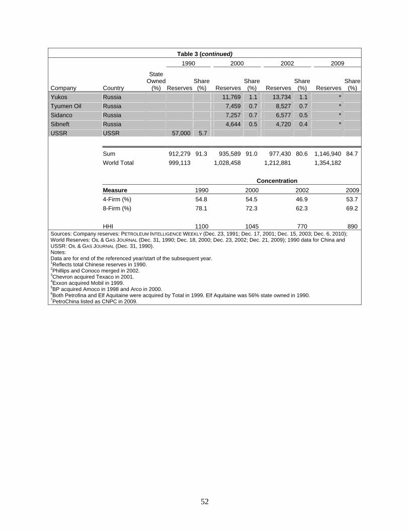
52
Table 3 (continued)
1990 2000 2002 2009
Company Country
State Owned
(%) ReservesShare
(%) ReservesShare
(%) Reserves Share
(%) ReservesShare
(%)
Yukos Russia 11,769 1.1 13,734 1.1 *
Tyumen Oil Russia 7,459 0.7 8,527 0.7 *
Sidanco Russia 7,257 0.7 6,577 0.5 *
Sibneft Russia 4,644 0.5 4,720 0.4 *
USSR USSR 57,000 5.7
Sum 912,279 91.3 935,589 91.0 977,430 80.6 1,146,940 84.7
World Total 999,113 1,028,458 1,212,881 1,354,182
Concentration
Measure 1990 2000 2002 2009
4-Firm (%) 54.8 54.5 46.9 53.7
8-Firm (%) 78.1 72.3 62.3 69.2
HHI 1100 1045 770 890 Sources: Company reserves: PETROLEUM INTELLIGENCE WEEKLY (Dec. 23, 1991; Dec. 17, 2001; Dec. 15, 2003; Dec. 6, 2010); World Reserves: OIL & GAS JOURNAL (Dec. 31, 1990; Dec. 18, 2000; Dec. 23, 2002; Dec. 21, 2009); 1990 data for China and USSR: OIL & GAS JOURNAL (Dec. 31, 1990). Notes: Data are for end of the referenced year/start of the subsequent year. 1Reflects total Chinese reserves in 1990. 2Phillips and Conoco merged in 2002. 3Chevron acquired Texaco in 2001. 4Exxon acquired Mobil in 1999. 5BP acquired Amoco in 1998 and Arco in 2000. 6Both Petrofina and Elf Aquitaine were acquired by Total in 1999. Elf Aquitaine was 56% state owned in 1990. 7PetroChina listed as CNPC in 2009.

53
Table 4: Concentration of World Crude Oil Reserves Country Basis Select Years 1990 - 2009
(Reserves in Millions of Barrels at Year End) 1990 2000 2002 2009
Country Reserves Share
(%) ReservesShare
(%) ReservesShare
(%) Reserves Share
(%) Saudi Arabia1 260,000 26.0 261,700 25.4 261,800 21.6 259,900 19.2 Iran 92,850 9.3 89,700 8.7 89,700 7.4 137,620 10.2 Iraq 100,000 10.0 112,500 10.9 112,500 9.3 115,000 8.5 Kuwait1 97,025 9.7 96,500 9.4 96,500 8.0 101,500 7.5 Venezuela 59,040 5.9 76,862 7.5 77,800 6.4 99,377 7.3 Abu Dhabi 92,200 9.2 92,200 9.0 92,200 7.6 92,200 6.8 Russia 48,573 4.7 60,000 4.9 60,000 4.4 Libya 22,800 2.3 29,500 2.9 29,500 2.4 44,270 3.3 Nigeria 17,100 1.7 22,500 2.2 24,000 2.0 37,200 2.7 Kazakhstan 5,417 0.5 9,000 0.7 30,000 2.2 Qatar 4,500 0.5 13,157 1.3 15,207 1.3 25,410 1.9 China 24,000 2.4 24,000 2.3 18,250 1.5 20,350 1.5 Brazil 2,840 0.3 8,100 0.8 8,322 0.7 12,802 0.9 Algeria 9,200 0.9 9,200 0.9 9,200 0.8 12,200 0.9 Mexico 51,983 5.2 28,260 2.7 12,622 1.0 10,404 0.8 Angola 2,074 0.2 5,412 0.5 5,412 0.4 9,500 0.7 Norway 7,609 0.8 9,447 0.9 10,265 0.8 6,680 0.5 India 7,997 0.8 4,728 0.5 5,367 0.4 5,625 0.4 Oman 4,300 0.4 5,506 0.5 5,506 0.5 5,500 0.4 Dubai 4,000 0.4 4,000 0.4 4,000 0.3 4,000 0.3 Malaysia 2,900 0.3 3,900 0.4 3,000 0.2 4,000 0.3 Indonesia 11,050 1.1 4,980 0.5 5,000 0.4 3,990 0.3 Egypt 4,500 0.5 2,948 0.3 3,700 0.3 3,700 0.3 United Kingdom 3,825 0.4 5,003 0.5 4,715 0.4 3,084 0.2 Yemen 4,000 0.4 4,000 0.4 4,000 0.3 3,000 0.2 Exxon2 3,584 0.4 4,319 0.4 4,194 0.3 2,144 0.2 USSR 57,000 5.7
Sum 946,377 972,412 971,760 1,109,456 World Reserves 999,113 1,028,458 1,212,881 1,354,182 Concentration
Measure 1990 2000 2002 2009 4-Firm (%) 55.0 54.7 46.4 45.3 8-Firm (%) 83.5 78.5 67.6 67.2 HHI 1156 1122 812 753 Sources: Country Crude Oil Reserves: OIL & GAS JOURNAL: (Dec. 31, 1990; Dec. 18, 2000; Dec. 23, 2002; Dec. 21, 2009); ExxonMobil's U.S. and Canadian crude oil reserves: Form 10-K filed annually with the SEC. Notes: 1 Reserves for Saudi Arabia and Kuwait each includes one-half of the Neutral Zone reserves. 2 Reserves in the U.S. and Canada

54
Table 5: OPEC Share of World Crude Oil and NGL Production Select Years 1974 - 2010
(Production in Thousand Barrels per Day) Country 1974 1980 1985 1990 1995 2000 2002 2005 2010
Saudi Arabia1 8,610 10,269 3,763 7,030 8,977 9,214 8,714 11,010 10,434 Iran 6,067 1,671 2,260 3,123 3,703 3,771 3,531 4,241 4,248 Venezuela 3,060 2,228 1,740 2,253 2,969 3,440 2,906 2,771 2,358
Kuwait1 2,596 1,751 1,077 1,240 2,152 2,194 2,019 2,659 2,450 Nigeria 2,255 2,055 1,495 1,810 1,993 2,165 2,118 2,627 2,455 Iraq 1,971 2,522 1,443 2,070 585 2,586 2,043 1,893 2,412 Libya 1,541 1,827 1,085 1,410 1,430 1,470 1,384 1,722 1,790
Indonesia6 1,375 1,647 1,369 1,539 1,579 1,513 1,347 1,135 - Algeria 1,059 1,142 1,157 1,305 1,347 1,484 1,576 2,092 2,079 Qatar 523 482 331 446 497 870 839 1,100 1,414
UAE2 2,032 1,744 1,353 2,252 2,393 2,568 2,382 2,835 2,804
Gabon3 202 175 172 270 - - - - -
Ecuador4 177 206 283 287 - - - - 487
Angola5 - - - - - - - - 1,988 OPEC 31,468 27,719 17,528 25,035 27,625 31,275 28,859 34,085 34,919 NON-OPEC 27,264 35,285 40,386 40,097 40,416 43,679 45,169 47,285 47,519 WORLD 58,732 63,004 57,914 65,132 68,041 74,954 74,028 81,370 82,438 OPEC Share (%) 53.6 44.0 30.3 38.4 40.6 41.7 39.0 41.9 42.4 Sources: 1974 Production: FTC, MERGERS IN THE U.S. PETROLEUM INDUSTRY 1971-1984: AN UPDATED COMPARATIVE ANALYSIS, Table 21, at 81-82; 1980-2010 Production: EIA, International Energy Statistics, Annual Petroleum Production, Production of Crude Oil: 1980-2010, & Production of NPGL: 1980-2010. Notes: 1Production for Saudi Arabia and Kuwait each includes one-half of the Neutral Zone production. 2United Arab Emirates, total of individual emirates' production. 3Gabon withdrew from OPEC in January 1995 and is not included in the 1995 OPEC total because reserve numbers are for year-end. 4Ecuador withdrew from OPEC in December 1992 and rejoined in 2007. 5Angola joined OPEC in 2007. 6Indonesia withdrew its membership in January 2009.

55
Table 6: OPEC Share of World Crude Oil Reserves Select Years 1973 - 2010
(Reserves in Billions of Barrels at Year End) Country 1973 1978 1981 1985 1990 1995 2000 2002 2010
Saudi Arabia1 140.8 168.9 167.9 171.5 260.0 261.2 261.7 261.8 262.6 Iraq 31.5 32.1 29.7 44.1 100.0 100.0 112.5 112.5 115.0
Kuwait1 72.8 69.4 67.7 92.5 97.0 96.5 96.5 96.5 104.0
Abu Dhabi2 21.5 30.0 30.6 31.0 92.2 92.2 92.2 92.2 92.2 Iran 60.0 59.0 57.0 47.9 92.9 88.2 89.7 89.7 137.0 Venezuela 14.0 18.0 20.3 25.6 59.0 64.5 76.9 77.8 211.2 Libya 25.5 24.3 22.6 21.3 22.8 29.5 29.5 29.5 46.4 Nigeria 20.0 18.2 16.5 16.6 17.1 20.8 22.5 24.0 37.2 Qatar 6.5 4.0 3.4 3.3 4.5 3.7 13.2 15.2 25.4 Algeria 7.6 6.3 8.1 8.8 9.2 9.2 9.2 9.2 12.2
Indonesia6 10.5 10.2 9.8 8.5 11.1 5.2 5.0 5.0 -
Dubai2 2.5 1.3 1.3 1.4 4.0 4.3 4.0 4.0 4.0
Sharjah2 1.5 0.0 0.3 0.5 1.5 1.5 1.5 1.5 1.5
Ras al-Khaimah2 0.0 0.0 0.0 0.1 0.4 0.1 0.1 0.1 0.1
Gabon3 1.5 2.0 0.5 0.5 0.7 - - - -
Ecuador4 5.7 1.2 0.9 1.7 1.4 - - - 6.5
Angola5 - - - - - - - - 9.5 TOTAL OPEC 421.9 444.9 436.6 475.3 773.8 776.9 814.5 819.0 1,059.8 TOTAL NON-OPEC 206.0 196.7 234.1 224.8 225.3 230.6 214.0 393.9 409.8 TOTAL WORLD 627.9 641.6 670.7 700.1 999.1 1,007.5 1,028.5 1,212.9 1,469.6 OPEC Share (%) 67.2 69.3 65.1 67.9 77.4 77.1 79.2 67.5 72.1 Sources: 1973-1981 Reserves: FTC, MERGERS IN THE U.S. PETROLEUM INDUSTRY 1971-1984: AN UPDATED COMPARATIVE ANALYSIS, Table 20 at 79; 1985-2009 Reserves: OIL & GAS JOURNAL (Dec. 30, 1985; Dec. 31, 1990; Dec. 25, 1995; Dec. 18, 2000; Dec. 23, 2002; Dec. 6, 2010). Notes: 1Reserves for Saudi Arabia and Kuwait include one-half on the Neutral Zone reserves. 2Individual Emirates of the United Arab Emirates; only Emirates that have crude oil reserves are listed. 3Gabon withdrew from OPEC in January 1995; it is not included in the 1995 OPEC total because reserve numbers are for year-end. 4Ecuador withdrew from OPEC in December 1992 and rejoined in 2007. 5Angola joined OPEC in 2007. 6Indonesia withdrew its membership in January 2009.

56
Table 7: U.S. Refinery Runs of Crude Oil by Source Select Years 1985 - 2010
(Thousand Barrels per Day)
Year
Domestic Crude Oil Production
U.S. Crude Oil Imports
U.S. Crude Oil Exports
Refinery Runs of
Crude Oil
Imports as % of Refinery
Runs 1985 8,971 3,201 204 12,044 27 1990 7,355 5,894 109 13,409 44 1995 6,560 7,230 95 13,973 52 2000 5,822 9,071 50 15,067 60 2003 5,681 9,665 12 15,304 63 2005 5,178 10,126 32 15,220 67 2009 5,361 9,013 44 14,336 63 2010 5,512 9,163 42 14,722 62 Sources: 1985 to 2003: EIA, PETROLEUM SUPPLY ANNUAL, Table S-2; 2005-2010: EIA, PETROLEUM SUPPLY ANNUAL 2009, Volume 1, Table 2;

57
Table 8: U.S. Crude Oil Imports by Country of Origin Select Years 2001- 2010
(Imports in Thousand Barrels per Year) 2001 2005 2010 Country Imports % of Total Imports % of Total Imports % of TotalCanada 494,796 14.5 596,183 16.1 719,698 21.5 Mexico 508,715 14.9 567,955 15.4 416,093 12.4 Saudi Arabia 588,075 17.3 527,287 14.3 394,280 11.8 Nigeria 307,173 9.0 393,038 10.6 359,801 10.8 Venezuela 471,243 13.8 452,914 12.3 332,926 10.0 Iraq 289,998 8.5 192,524 5.2 151,117 4.5 Angola 117,254 3.4 166,404 4.5 138,755 4.1 Colombia 94,844 2.8 57,002 1.5 123,525 3.7 Kuwait 86,535 2.5 82,730 2.2 71,275 2.1 United Kingdom 89,142 2.6 81,621 2.2 43,873 1.3 Norway 102,724 3.0 43,454 1.2 9,201 0.3 Other 254,395 7.5 534,859 14.5 583,941 17.5 Total 3,404,894 100.0 3,695,971 100.0 3,344,485 100.0 Sources: 2001: EIA, PETROLEUM SUPPLY ANNUAL, Table 21 (2001); 2005 & 2010: EIA, Petroleum, U.S. Imports by Country of Origin (2005, 2010).

58
Table 9: Number of Operable U.S. Refineries, Total Capacity, Average Capacity Utilization
Select Years 1949 - 2011 (Thousand Barrels per Day)
Year Number Total
Capacity Average
Refinery CapacityUtilization
(%) 1949 336 6,230 18.5 89.2 1950 320 6,220 19.4 92.5 1955 296 8,390 28.3 92.2 1960 309 9,840 31.8 85.1 1965 293 10,420 35.6 91.8 1970 276 12,020 43.6 92.6 1975 279 14,960 53.6 85.5 1980 319 17,990 56.4 75.4 1985 223 15,660 70.2 77.6 1990 205 15,570 76.0 87.1 1991 202 15,680 77.6 86.0 1992 199 15,700 78.9 87.9 1993 187 15,120 80.9 91.5 1994 179 15,030 84.0 92.6 1995 175 15,430 88.2 92.0 1996 170 15,330 90.2 94.1 1997 164 15,450 94.2 95.2 1998 163 15,710 96.4 95.6 1999 159 16,260 102.3 92.6 2000 158 16,510 104.5 92.6 2001 155 16,600 107.1 92.6 2002 153 16,790 109.7 90.7 2003 149 16,760 112.5 92.5 2004 149 16,890 113.4 93.0 2005 148 17,120 115.7 90.6 2006 149 17,340 116.4 89.7 2007 149 17,440 117.0 88.5 2008 150 17,590 117.3 85.3 2009 150 17,670 117.8 82.8 2010 148 17,580 118.8 83.7 2011 148 17,740 119.9
Sources: 1949-2009 capacity and utilization data: Refinery Capacity and Utilization, 1949-2009. EIA, ANNUAL ENERGY REVIEW 2009, Table 5.9; 2010-2011 capacity data: EIA REFINERY CAPACITY REPORT (2010, 2011), Table 1; 2010 utilization data: EIA, PETROLEUM SUPPLY MONTHLY, December 2010, Table 4. Note: Total capacity per calendar day on January 1.

59
Table 10: Number of Operable Refineries and Refining Capacity by PADD
Select Years 2004 - 2011 Year Refinery Data PADD I PADD II PADD III PADD IV PADD V U.S. Total2004 Number 16 26 55 16 36 149 Capacity 1.74 3.53 7.88 0.58 3.16 16.89 % of U.S. Capacity 10.2 20.9 46.7 3.4 18.7 2007 Number 15 26 56 16 36 149 Capacity 1.72 3.59 8.35 0.60 3.19 17.45 % of U.S. Capacity 9.9 20.6 47.9 3.4 18.3 2011 Number 14 27 56 17 34 148 Capacity 1.62 3.72 8.65 0.62 3.13 17.74 % of U.S. Capacity 9.1 21.0 48.8 3.5 17.6 Sources: 2004: EIA, PETROLEUM SUPPLY ANNUAL (2004), Table 36; 2007, 2011 EIA, REFINERY CAPACITY REPORT (2007, 2011), Table 1. Note: Capacity is in millions of barrels per calendar day on January 1.

60
Table 11: Inter-PADD Shipments and Imports Finished Light Petroleum Products1 - 2005
(Thousand barrels) PADD I II III IV V U.S. Refinery Production2 508,506 1,073,358 2,240,929 172,955 856,721 4,852,469Other Production3 1,801 92,179 28,176 226 184 120,765 Imports 490,117 2,579 58,409 2,662 56,775 610,402Exports 7,955 5,144 109,633 8 19,780 142,535Net Imports 482,162 -2,565 -51,224 2,654 36,995 467,867 Receipts from other PADDs4 PADD I - 123,058 708 0 708 124,474PADD II 10,556 - 17,993 9,197 0 37,746PADD III 1,069,533 327,890 - 12,672 40,807 1,450,902PADD IV 0 10,880 0 - 11,893 22,773PADD V 0 0 792 0 - 792Receipts from other PADDs 1,080,089 461,828 19,493 21,869 53,408 1,636,687Deliveries to other PADDs 124,474 37,746 1,450,902 22,773 792 1,636,687Net Receipts from other PADDs 955,615 424,082 -1,431,409 -904 52,616 0 Stock Change5 -549 1,714 -592 -1,040 819 352 Product Supply6 1,968,961 1,545,456 793,180 178,151 973,289 5,459,036 Percentage of Product Supply Refinery Production 25.8 69.5 282.5 97.1 88.0 88.9 Other Production 0.1 6.0 3.6 0.1 0.0 2.2 Net Imports 24.5 -0.2 -6.5 1.5 3.8 8.6 Net Receipts from other PADDs 48.5 27.4 -180.5 -0.5 5.4 0.0 Stock Change 0.0 0.1 -0.1 -0.6 0.1 0.0 From Outside PADD 73.0 27.3 -186.9 1.0 9.2 8.6 Source: EIA, data from http://www.eia.gov/petroleum/data.cfm#summary. Notes: EIA data includes data from Refinery Net Production; Refinery Net Input; Oxygenate Net Production; Imports by Area of Entry, Exports; Movements Between PAD Districts by Pipeline, Tanker, and Barge; Total Stocks; and Product Supplied. 1Light refined products are motor gasoline, jet fuel and distillate fuel oil. 2Refinery Production includes refinery net output of finished motor gasoline, jet fuel, and distillate fuel oil, minus refinery net inputs of gasoline blending components. 3Other production is production of oxygenates including ethanol. 4Receipts from other PADDs includes shipments by pipeline, tanker and barge, but does not include shipments by rail or truck, the main methods of shipping ethanol. Therefore, net receipts for PADDs that are net recipients of ethanol will be biased downwards. Similarly, net receipts of PADDs are net suppliers of ethanol will be biased upwards. 5A positive stock change denotes an increase in stocks; a negative stock change denotes a decrease in stocks. Distillate stocks in the Northeast Heating Oil Reserve are not included. 6Product supply includes refinery and blender net production, other production, net imports, net receipts from other PADDs, and stock change.

61
Table 12: Inter-PADD Shipments and Imports Finished Light Petroleum Products1 - 2010
(Thousand barrels) PADD I II III IV V U.S. Refinery Production2 374,007 1,085,439 2,413,983 174,247 781,377 4,829,053Other Production3 7,062 292,804 20,187 4,989 3,475 328,517 Imports 367,029 3,546 35,669 2,157 32,349 440,748Exports 25,333 4,342 362,952 28 41,042 413,166Net Imports 341,696 -796 -327,283 2,129 -8,693 27,582 Receipts from other PADDs4 PADD I - 110,970 435 0 435 111,840PADD II 15,461 - 28,925 21,919 0 66,305PADD III 1,059,369 199,268 - 9,425 55,930 1,323,992PADD IV 0 10,917 0 - 11,548 22,465PADD V 0 0 0 0 - 0Receipts from other PADDs 1,074,830 321,155 29,360 31,344 67,913 1,524,602Deliveries to other PADDs 111,840 66,305 1,323,992 22,465 0 1,524,602Net Receipts from other PADDs 962,990 254,850 -1,294,632 8,879 67,913 0 Stock Change5 -15,475 -2,966 9,599 2,060 1,858 -4,924 Product Supply6 1,810,863 1,439,585 866,091 189,807 895,517 5,201,862
Percentage of Product Supply Refinery Production 20.7 75.4 278.7 91.8 87.3 92.8 Other Production 0.4 20.3 2.3 2.6 0.4 6.3 Net Imports 18.9 -0.1 -37.8 1.1 -1.0 0.5 Net Receipts from other PADDs 53.2 17.7 -149.5 4.7 7.6 0.0 Stock Change -0.9 -0.2 1.1 1.1 0.2 -0.1 From Outside PADD 72.0 17.6 -187.3 5.8 6.6 0.5 Source: EIA, data from http://www.eia.gov/petroleum/data.cfm#summary. Notes: EIA data includes data from Refinery Net Production; Refinery Net Input; Oxygenate Net Production; Imports by Area of Entry, Exports; Movements Between PAD Districts by Pipeline, Tanker, and Barge; Total Stocks; and Product Supplied. 1Light refined products are motor gasoline, jet fuel and distillate fuel oil. 2Refinery Production includes refinery net output of finished motor gasoline, jet fuel, and distillate fuel oil, minus refinery net inputs of gasoline blending components. 3Other production is production of oxygenates including ethanol. 4Receipts from other PADDs includes shipments by pipeline, tanker and barge, but does not include shipments by rail or truck, the main methods of shipping ethanol. Therefore, net receipts for PADDs that are net recipients of ethanol will be biased downwards. Similarly, net receipts of PADDs are net suppliers of ethanol will be biased upwards. 5A positive stock change denotes an increase in stocks; a negative stock change denotes a decrease in stocks. Distillate stocks in the Northeast Heating Oil Reserve are not included. 6Product supply includes refinery and blender net production, other production, net imports, net receipts from other PADDs, and stock change.

62
Table 13: Regional Refining Concentration Trends Select Years 1985 - 2010
PADD 1985 1990 1996 2000 2003 2006 2010
U.S.
4-Firm (%) 34.4 31.4 27.3 40.2 44.4 45.9 41.8
8-Firm (%) 54.6 52.2 48.4 61.6 69.4 69.9 67.4
HHI 493 437 412 611 728 759 680
PADD I
4-Firm (%) 50.9 59.2 75.5 80.7 76.7 90.7 96.4
8-Firm (%) 83.7 88.7 93.8 99.0 97.9 100.0 100.0
HHI 995 1225 2001 2158 1943 2707 3255
PADD II
4-Firm (%) 41.1 39.3 40.9 50.9 57.1 55.2 46.3
8-Firm (%) 64.4 65.0 67.3 75.6 82.6 80.8 70.7
HHI 681 675 721 961 1063 1040 833
PADD III
4-Firm (%) 39.2 36.3 35.1 48.4 56.3 60.7 54.9
8-Firm (%) 58.1 58.5 58.1 66.5 78.8 81.0 77.9
HHI 599 578 576 851 1018 1106 972
PADD IV
4-Firm (%) 57.3 55.8 55.0 58.1 46.1 50.6 51.8
8-Firm (%) 82.7 83.6 84.4 86.9 81.2 84.8 85.2
HHI 1093 1080 1129 1179 944 1021 1048
PADD V
4-Firm (%) 58.0 53.8 54.0 60.2 62.4 62.4 67.1
8-Firm (%) 79.6 74.2 79.5 86.9 92.7 90.5 94.0
HHI 1248 965 1034 1148 1246 1220 1364
Upper Midwest1
4-Firm (%) 56.5 54.7 57.4 75.6 75.2 74.8 69.9
8-Firm (%) 86.9 87.9 90.7 99.8 99.8 100.0 98.8
HHI 1085 1102 1177 1756 1732 1949 1646
California
4-Firm (%) 60.2 58.9 61.4 68.7 66.2 63.8 68.9
8-Firm (%) 81.5 82.5 89.6 95.1 96.3 93.7 98.1
HHI 1431 1184 1335 1481 1475 1393 1600
PADDs I & III
4-Firm (%) 38.4 36.7 32.2 44.6 54.6 58.2 52.4
8-Firm (%) 57.3 57.2 55.3 65.3 76.1 79.7 74.5
HHI 573 561 514 741 919 1017 868
PADDs II & III
4-Firm (%) 33.4 30.7 31.7 42.5 46.2 50.6 45.4
8-Firm (%) 53.3 56.5 53.0 64.9 75.6 77.7 73.6
HHI 469 455 485 681 826 873 781
PADDs I, II, III
4-Firm (%) 32.8 30.2 29.8 39.4 45.9 50.1 44.5
8-Firm (%) 54.4 53.6 51.4 63.5 73.1 76.3 71.0
HHI 469 460 460 638 789 858 737 Sources: Capacity 1985-2003: EIA, PETROLEUM SUPPLY ANNUAL, Table 38 (1985, 1990, 1996, 2000, 2003); Capacity 2006 and 2010: EIA, REFINERY CAPACITY REPORT (2007, 2011). Notes: Capacities are crude oil distillation capacity measured per calendar day at the end of the year. 1The Upper Midwest consists of Illinois, Indiana, Kentucky, Michigan, and Ohio.

63
Table 14: Wholesale Concentration Estimates 2003 - 2010
(HHI Measure)
State 2003 2004 2005 2006 2007 2008 2009 2010
PADD I-A
Connecticut 1,514 1,406 1,320 1,260 1,272 1,375 1,269 1,228
Maine 1,468 1,561 1,524 1,511 1,317 1,749 1,665 1,813
Massachusetts 1,474 1,435 1,270 1,352 1,221 1,178 1,203 1,255
New Hampshire 1,163 1,176 1,094 1,275 1,426 1,482 1,448 1,422
Rhode Island 1,736 1,503 1,416 1,193 1,374 1,646 1,728 2,121
Vermont 1,264 1,144 1,106 1,314 1,667 1,501 1,263 1,263
PADD I-B
Delaware 1,453 1,433 1,664 1,588 1,894 1,888 1,419 1,471
Dist. Of Col. 2,616 2,516 2,937 3,049 3,470 2,820 2,672 2,739
Maryland 1,258 1,367 1,332 1,310 1,332 1,186 1,141 1,159
New York 1,098 1,094 1,025 959 930 882 901 800
New Jersey 1,149 1,124 1,154 1,086 1,087 1,027 971 1,013
Pennsylvania 1,429 2,045 1,550 1,767 2,040 1,897 1,443 1,834
PADD I-C
Florida 994 964 997 836 839 912 861 869
Georgia 1,176 1,158 1,088 1,092 1,107 1,121 1,023 1,029
North Carolina 1,215 1,140 1,106 1,069 1,014 995 1,012 1,228
South Carolina 1,013 968 971 923 950 913 923 1,093
Virginia 1,148 1,188 1,223 1,144 1,098 1,021 982 1,145
West Virginia 1,511 1,435 1,524 1,603 1,580 1,588 1,502 1,537
PADD II
Illinois 1,316 1,312 1,318 1,287 1,313 1,304 1,392 1,364
Indiana 2,140 2,090 2,344 2,213 2,228 2,091 2,236 2,279
Iowa 1,122 1,020 1,179 1,145 1,010 918 1,010 819
Kansas 1,557 1,220 1,199 1,269 1,192 1,251 1,274 1,254
Kentucky 2,403 2,639 2,744 2,820 3,276 3,412 3,258 3,846
Michigan 1,916 1,952 2,012 2,113 2,222 2,199 2,134 1,973
Minnesota 1,404 1,400 1,414 1,524 1,824 1,598 1,579 1,547
Missouri 1,283 1,306 1,294 1,280 1,343 1,372 1,351 1,489

64
Table 14 (continued)
Nebraska 1,669 1,333 1,454 1,300 1,322 1,244 1,387 1,136
North Dakota 2,539 1,860 2,650 2,068 2,608 3,164 2,807 2,196
Ohio 1,971 1,986 2,073 2,099 2,287 2,056 2,284 2,197
Oklahoma 1,315 1,248 1,348 1,371 1,219 1,358 1,341 1,309
South Dakota 1,204 1,199 1,100 990 1,047 846 901 920
Tennessee 1,251 1,234 1,110 1,111 1,101 1,096 1,110 1,172
Wisconsin 1,352 1,405 1,319 1,439 1,399 1,414 1,473 1,386
PADD III
Alabama 1,136 1,125 1,125 1,133 1,134 1,151 1,158 1,257
Arkansas 977 967 983 980 1,007 1,021 1,046 1,007
Louisiana 1,160 1,096 1,095 1,134 1,110 1,162 1,219 1,218
Mississippi 1,046 1,039 1,062 962 1,071 1,017 1,070 1,140
New Mexico 1,465 1,467 1,555 1,447 1,418 1,341 1,476 1,450
Texas 1,138 1,125 1,067 1,107 1,127 1,187 1,042 1,040
PADD IV
Colorado 1,395 1,389 1,403 1,631 1,693 1,627 1,688 1,838
Idaho 1,277 1,276 1,230 1,125 1,037 1,059 998 1,051
Montana 2,234 2,304 2,349 1,628 1,660 1,750 1,677 1,704
Utah 1,529 1,540 1,350 1,440 1,475 1,451 1,524 1,555
Wyoming 1,287 1,288 1,222 1,188 1,171 1,259 1,402 1,439
PADD V
Alaska 2,918 2,878 3,126 3,335 3,080 3,299 3,299 3,243
Arizona 1,058 1,043 989 947 977 1,021 1,046 1,007
California 1,601 1,382 1,358 1,292 1,324 1,318 1,329 1,302
Hawaii 3,365 4,305 4,460 2,765 2,756 2,860 2,854 3,423
Nevada 1,745 1,714 1,568 1,301 1,602 1,585 1,463 1,392
Oregon 1,768 1,749 1,795 1,831 1,682 1,726 1,758 1,640
Washington 1,608 1,622 1,582 1,483 1,544 1,561 1,500 1,466 Source: EIA estimates provided to FTC staff, based on EIA, Form 782-C, Prime Supplier Sales (monthly). Note: Concentration estimates are for December of each listed year.

65
Table 15: Refiner Disposition of Gasoline by Class of Trade (% by Class) 2002 - 2010
PADD
Total Gas Volume for All Grades and
Formulations US I I-A I-B I-C II III IV V
2002 Co-op 18.8 17.6 13.9 17.4 18.5 17 18.3 19.9 23.7 DTW 20.2 24.7 33.1 41.8 11.2 7.9 2.8 8.4 49.2 Rack 61.0 57.7 53 40.8 70.3 75.1 78.9 71.7 27.0 Total Volume1 330,594 110,150 12,073 39,974 58,103 98,238 51,156
2003 Co-op 18.8 18.0 13.6 18.6 18.4 17.5 17.9 19.5 23.3 DTW 18.1 21.7 29.6 37.2 9.4 6.1 2.3 9.2 47.3 Rack 63.1 60.3 56.7 44.1 72.2 76.4 79.8 71.4 29.4 Total Volume1 330,436 110,626 12,259 40,024 58,343 98,342 51,241 11,769 58,458
2004 Co-op 17.3 16.2 13.8 17.8 15.5 17.3 16.6 - - DTW 16.7 19.3 27.6 33.2 8.0 4.4 1.9 - - Rack 66.0 64.5 58.6 49.0 76.5 78.4 81.5 - - Total Volume1 328,734 108,770 11,637 39,885 57,248 99,061 50,505 - -
2005 Co-op 17.4 16.5 15.5 17.9 15.7 17.1 17.4 - - DTW 14.7 15.8 25.1 27.0 6.5 3.3 1.5 - - Rack 67.8 67.7 59.5 55.1 77.8 79.6 81.0 - - Total Volume1 330,482 108,668 11,855 38,626 58,187 97,175 52,567 - -
2006 Co-op 17.7 17.0 16.8 18.3 16.3 17.4 17.8 - - DTW 13.4 14.1 23.6 24.2 5.4 2.6 1.3 - - Rack 68.9 68.9 59.6 57.5 78.4 80.0 80.9 - - Total Volume1 330,892 108,722 11,788 38,553 58,382 95,510 53,919 - -
2007 Co-op 17.3 17.1 18.1 18.4 16.0 16.9 17.8 - - DTW 13.1 13.7 23.9 24.4 4.8 2.4 1.1 - - Rack 69.5 69.2 58.0 57.3 79.2 80.7 81.0 - - Total Volume1 327,249 106,894 11,171 37,914 57,808 93,621 55,221 - -
2008 Co-op 17.1 17.1 16.9 17.4 16.9 16.6 17.6 - - DTW 12.7 13.2 19.0 23.6 4.8 2.3 0.9 - - Rack 70.2 69.7 64.1 59.0 78.3 81.2 81.5 - - Total Volume1 314,572 100,908 10,911 37,000 52,997 89,827 54,961 - -
2009 Co-op 15.3 15.7 16.4 16.6 15.0 14.5 18.0 9.1 14.6 DTW 12.7 12.1 17.9 23.0 3.5 1.9 0.3 1.6 45.2 Rack 72.0 72.2 65.7 60.4 81.6 83.6 81.7 89.3 40.2 Total Volume1 313,942 101,548 10,713 37,147 53,688 90,661 52,368
2010 Co-op 13.8 14.4 - - 12.9 12.4 18.1 - - DTW 11.4 9.8 - - 1.9 0.7 0.3 - - Rack 74.7 75.8 - - 85.2 86.9 81.7 - - Total Volume1 311,642 98,892 - - 53,989 90,688 52,717 - - Source: EIA Form 782-A, Refiners'/Gas Plant Operators' Monthly Petroleum Products Sales Report (monthly). Notes: 2002 annual DTW data withheld for PADDs IV and V; June, August, October 2002 data are used as a proxy. 2004 – 2008 annual DTW data withheld for PADDs IV and V, therefore no total volume is available to calculate percentage in class of trade. 2009 annual DTW withheld for PADD IV and V; monthly volume for April, May, June, September are averaged as a proxy for 2009 DTW and total volume. 2010 Some monthly DTW and Rack data withheld for PADDs IA, IB, IV, and V, therefore no total volume is available to calculate percentage in class of trade. 1Total volume is in thousand gallons per day.