gas peak design day analysis - core scholar
TRANSCRIPT
Wright State UniversityCORE Scholar
Economics Student Publications Economics
1994
Gas Peak Design Day AnalysisKerry Elaine BroehlWright State University - Main Campus
Follow this and additional works at: https://corescholar.libraries.wright.edu/econ_student
Part of the Business Commons, and the Economics Commons
This Master's Culminating Experience is brought to you for free and open access by the Economics at CORE Scholar. It has been accepted for inclusionin Economics Student Publications by an authorized administrator of CORE Scholar. For more information, please [email protected], [email protected].
Repository CitationBroehl, K. E. (1994). Gas Peak Design Day Analysis. .https://corescholar.libraries.wright.edu/econ_student/46

GAS PEAK DESIGN DAY ANALYSIS
An internship report submitted in partial fulfillment of the requirements for the degree of
Master of Science
By
KERRY ELAINE BROEHL B.A., Miami University, 1991
1994Wright State University
WRIGHT STATE UNIVERSITY
DEPARTMENT OF ECONOMICS
JULY 26, 1994
I HEREBY RECOMMEND THAT THE INTERNSHIP REPORT PREPARED UNDER MY SUPERVISION BY Kerry Elaine Broehl ENTITLED Gas Peak Design Day Analysis BE ACCEPTED IN PARTIAL FULFILLMENT OF THE REQUIREMENTS FOR THE DEGREE Master of Science.
Director, M.S. in Social and Applied Economics
ABSTRACT
Broehl, Kerry Elaine. M.S., Department of Economics, Wright State University, 1994.Gas Peak Design Day Analysis.
The changing natural gas industry has increased the importance for utility
companies to develop an accurate peak day forecast. The model developed for this
midwest utility estimates a firm natural gas sendout econometrically, using the Ordinary
Least Squares regression analysis. The peak is primarily weather driven, thus the model
made use of wind-chill variables from the current day, the previous day, and the current
day squared. Also included is a disposable income variable to reflect the level of economic
activity.
The peak day forecast depends on using extreme weather conditions for the design
day parameters. The parameters used represented the second worst wind-chill for the
utility's service area to occur in the last thirty years of history. The forecasted peak for the
1993/1994 winter season is calculated from the model to be 515,654 MCF, or 530,092
DTH. The actual peak occurrence for this season fell on January 18, 1994 where firm
sendout reached an all-time high of 513,876 MCF, or 528,261 DTH.

TABLE OF CONTENTS
Page
I. INTRODUCTION ....................................................................................... 1
II A CRITICAL REVIEW OF FORECASTING LITERATURE ................... 6
m . MODEL SPECIFICATION AND DATA REQUIREMENTS .................... 14
IV. EVALUATION OF MODEL RESULTS .................................................... 20
V. SUMMARY AND CONCLUSIONS ............... 26
iv
INTRODUCTION
The use of natural gas as an energy source has grown considerably in the last ten
years. It has been less expensive relative to alternate fuel sources, as well as emitting less
pollution and being abundant in supply. This strong growth in the natural gas industry has
prompted the movement towards government deregulation. Deregulation can occur
because the cost of entry is low enough to prompt much competition to avoid a natural
monopoly. As late as 1984, roughly ninety percent of the gas traveling in the interstate
pipeline system was gas sold by the FERC's (Federal Energy Regulatory Commission)
regulated interstate pipeline companies to local distribution companies for resale. For the
remaining ten percent of throughput on the interstate system, the Commission regulated
access to the interstate pipeline for "transportation only" service, and set the price for such
service. Transportation service allows the end-use customer to directly purchase their gas
from the pipeline company and have it transported through any necessary pipelines across
the United States to reach the end-use customer. This method by-passes the local utility
or distribution company. The result was the demand for natural gas on the interstate
system exceeded the supply. This was the motivating factor towards deregulation.
The first step was the Natural Gas Policy Act of 1978, which allowed for a slow
deregulation of well head prices and permitted the relaxation of regulation on the use of
gas transportation on the interstate pipeline. This began to make the gas transportation
service more accessible than the pervious ten percent limitation. By around 1990, FERC
Orders 436 and 500 had removed most of the legal barriers preventing the independent
transportation of natural gas. The barrier remaining, however, prevented a local
distribution company or an industrial end-user from buying gas directly from the producer
and having that gas delivered to the point of use each day.1
In the natural gas transportation service, there is a finite limit to the amount of gas
that can be transported through a pipeline at any given time. The FERC will not let
interstate pipelines contract on a firm (guaranteed) basis for more gas to be delivered on a
given day to a given point than what the pipeline is capable of delivering. It is unlikely,
however, that on any given day all firm customers of an interstate pipeline will want to
make full use of their maximum throughput. The un-utilized firm contract space in the
pipeline (along with any uncontracted space) is then open for use on an interruptible basis
to other customers. The interruptible's would have to leave the system if the firm
customers want to use their entire space. There is risk involved with using the
interruptible natural gas service, which is reflected in the lower price. Interruption,
however, is only likely to occur on an extreme peak day. Most interruptible customers are
prepared with a back-up alternate fuel source to help alleviate the risk.
The most recent and drastic deregulation measures has occurred with the
implementation of the FERC Order 636, effective November 1, 1993. This act is intended
to ensure that pipelines would provide a transportation service that was equal in quality
for all gas supplies, regardless of whether or not the customer purchases the gas from the
pipeline. Order 636 has called for an unbundling of the natural gas services. One required
unbundling was of sales and transportation services as far upstream as possible. Also, the
pipelines were now permitted to adopt market-based sales pricing. The result is that the
pipelines must offer firm and interruptible open-access storage in a non-discriminatory
manner.2 The natural gas industry mix of sales has now moved quickly from firm system
sales from the local utility or distribution center to transportation service sales directly to
the end-use customer.
With this increase in end-user transportation, local utilities are no longer providing
the traditional merchant function for a segment of their customer base. As a result, the
utility must constantly review its firm requirements in its system supply portfolio to
provide the least cost purchasing alternatives for system supply needs. An important
2

aspect to evaluate of the system supply needs is the amount necessary to cover a peak day.
The interstate pipeline firm transportation customers and those with firm sales through the
local utility will tend to make full use of their maximum throughput on a peak day. It is
not likely to have much excess for interruptible customers. It is the responsibility of the
utility to secure the gas necessary to cover the maximum throughput stated in each
customer's firm system sales contract. A peak day will occur when weather conditions are
extreme. The industrial load factor will increase only slightly, however, the commercial,
public authority, and residential sectors will increase considerably for they are the most
temperature sensitive. The obligation of the utility consists of two groups of customers.
The first is contracted on the system supply of the utility. This group of customers still
allows the local utility to contract the natural gas from the pipeline company. The utility
then sells it to the customer. This group consists of all the smaller customers, such as
residential, commercial, and small industry. It is not economical to contract their own gas
and transport. The second group consists of the human needs customers who transport
their natural gas, but need a back up insurance in the event that the gas does not arrive.
The sum of these two groups gives the utility's system supply obligation.
Contracts with the pipelines are secured several months in advance to the heating
season, thus a forecast of peak day requirements is necessary. The level of security must
by decided upon, such as to design for the worst day in the past thirty years, twenty years,
second worst day, etc. Regardless, the forecast must be as accurate as possible to be the
most cost effective. The firm sales arrangements between the interstate pipelines and local
distribution companies generally require payment of pipeline space reservation fees
(demand fees). There are also capacity securing costs. If the forecast is too high, then the
utility spends too much money on capacity and space contracts for gas not needed.
However, if the forecast is too low, then on peak day, there will be more gas demanded
than the contracts will supply. In order to fill its obligation and prevent breaching its
contracts to its customers, the utility must buy gas on the spot market, which proves to be
3
more expensive. It is extremely risky for the utility must purchase enough gas to meet its
needs at the same time many other utilities are doing the same. Competition can be stiff,
driving prices even higher. This could prove to be disastrous not only in high gas costs,
but also in lawsuits and bad publicity. The goal is to contract the most cost effective level,
taking all benefits and costs of being too high versus too low into consideration.
The model developed to forecast the natural gas peak estimates a firm natural gas
sendout equation econometrically, using the Ordinary Least Squares (OLS) regression
analysis. It has been determined that the peak is driven mainly by weather with a small
impact from the level of economic activity of the service area. The variables chosen to
drive the peak level consist of the current day wind-chill, the previous day wind-chill, and
the real disposable income of the service area. A non-linear functional equation was used
which included the square of the current day wind-chill. This allows the model to capture
the leveling off of the usage at extreme temperatures, a phenomenon called the "bendover"
effect. The peak is found by plugging extreme weather conditions into the estimated
equation, which will result in a peak firm sendout value. The data used was obtained from
a utility company located in the Midwest.
The expected results of the coefficient estimates for the current day and the
previous day wind-chill variables are to be negative. The extreme weather conditions
considered for this model tend to be negative. This multiplied by a negative coefficient
will result in a positive impact of the firm natural gas sendout. The current day wind-chill
squared variable is expected to have a negative impact. Due to the nature of a squared
variable, its value will always be positive. A negative coefficient will be necessary to allow
for a negative impact on firm sendout. This will capture the theory that the demand is
increasing at a decreasing rate. It is leveling off. Finally, the coefficient for the real
disposable income variable should be positive. A higher level of economic activity will
tend to drive the peak upwards.
4

The implications of this model are crucial for those in the utility industry involved
with the gas supply planning department. This group must negotiate and secure the
natural gas contracts for the utility with the pipelines. The most cost effective mix of
contracts to reach the forecasted peak level is the goal. The winter season peak
requirements will be met through the utility's utilization of its interstate pipeline
transportation and storage services, warranted firm supply agreements, company propane
peak-shaving volumes, and/or, when necessary, authorized excess services from interstate
pipelines. This peak forecast is also filed with the Public Utility Commission of the state.
At this point, the Commission's staff will investigate the validity and reasonableness of the
model and the results it produces. Finally, this model is also open for scrutiny from
various Gas Cost Recovery (GCR) auditors who are assigned to the utility by the
Commission to review all aspects of the utility's gas industry. This review will produce
recommendations of how much of the costs to the utility due to the natural gas industry
are recoverable from the government. The peak design day model is one of the aspects
reviewed.
The contents of this paper will discuss the development of this model, as well as
the results. Chapter one will provide a critical review of relevant literature on energy
forecasting. It will also discuss the gas peak model previously used by the utility. Chapter
two will present the model along with the data utilized. Chapter three will discuss the
estimation of the model and present the results. Also included is various testing of the
statistical validity of the model. The final chapter, Chapter four, will provide a summary
and conclusion for the paper.
5
A CRITICAL REVIEW OF FORECASTING LITERATURE
In order to design a forecasting model, it is essential to pick the best method for
the utility, as well as for the topic of analysis. There are several criterion for the selection
and evaluation of a forecasting technique. The top criterion considered are the sensibility
of the forecast, data availability and cost, historical performance of the model, evaluation
of structural change, explainability, and statistical validity, just to name a few of the
important ones. The next step is to evaluate the various forecasting techniques against the
criterion to find a good match. The first technique to evaluate is the trend extrapolation.
This method includes straight-line, polynomial, and logarithmic extrapolations where the
basic fit of historical data is obtained using techniques such as least-squares minimization.3
Because this method relies solely on past dependent variables, it is not a useful technique
for the gas peak model, which relies heavily on the weather to gas sendout relationship. It
also has no aspect to capture any sudden changes in growth. Although this technique
ranks high with respect to cost, minimal data requirements, and reproducibility, it was not
used in this analysis.
Another technique reviewed was the advanced time series model such as Box
Jenkins, moving average, exponential smoothing, and several others. These are based only
on a time dimension, but also has the ability to incorporate trends, seasonals, and cycles.4
Again, the ability to capture the extreme weather impacts is not strong in this method.
Other non-statistical methods can include expert judgment, which includes interviews with
utility personnel, consultants, and government experts to gather opinions of future sales
and peaks, and can also include customer surveys to obtain their expectations of their
future consumption. Although expert judgment is used here to help determine the
reasonableness of the forecast, the above techniques were not fully utilized.
6

Moving to the mainstream of techniques, those most popular with the utilities for
forecasting peak loads are end-use, econometric, and traditional load factor. The load
factor analysis is based on forecasting a load factor from historical data and anticipated
building schedules and then applying this load factor to the forecasted energy. The
equations used are:
Load Factor = Annual Energy Peak Hour * 8,760
Peak Hour Forecast = Annual Energy ForecastLoad Factor Forecast * 8,760
The load factor equation, based on historical data, gives a ratio of actual annual energy
usage to the peak or maximum load. In order for the two components to be spread over
the same time frame, the peak hour value must be multiplied by the number of hours in a
year.5 The load factor will give a percentage of what the actual annual usage is compared
to the maximum usage that would occur if the peak level were sustained throughout the
year. This percentage factor may change throughout the forecast period due to expected
growth (anticipated building schedules). To forecast the peak, the annual energy forecast
is now divided by the load factor forecast multiplied by the number of hours in a year.
Because the annual energy forecast for the utility is developed econometrically using
economic and weather variables, both variables are indirectly represented in the peak
calculated by the load factor technique. However, in this technique, the peak will vary
considerably from year to year, depending on how severe the weather happened to be for
that winter season. This will have little impact on the annual energy for that year due to
the many other determining variables. This will cause the load factor to be extremely
volatile throughout history, thus making a future prediction difficult. Another setback for
this technique is that the peak day extreme weather conditions to be used in forecasting
the peak level may be outside the realm of the data sample. A scaling factor would need
7

to be implemented to compensate for the difference. This introduces more uncertainty
into the model, thus this technique was not utilized.
The next common peak forecasting technique is through evaluating the end-use
equipment. An end-use methodology forecasts energy consumption by focusing on the
stock of energy-using equipment. In the residential sector, these models are characterized
by forecasts by appliance. Here, the number of households multiplied by the appliance
saturation multiplied by the use per appliance results in consumption per appliance. In the
commercial and industrial sector, these forecasts are generally done by equipment type
such as heaters, boilers, furnaces, lighting, and motors.6 An end-use analysis requires
large amounts of detailed data, which is time-consuming and expensive to collect and
update periodically. Also, while the end-use approach tends to work well in the residential
sector, in the commercial and industrial sectors, because the end-uses are not
homogeneous, the end-use approach requires special techniques, including more detailed
research. Some companies have overcome the data problem by using non-service area
data obtained from government agencies or purchasing from other utilities. This data,
however, no longer reflects the conditions of the service area being evaluated.
To best represent the specific conditions of the utility's service area in the most
cost effective manner, the econometrics approach was chosen for the peak model.
Econometrics is a method of quantitative measurement of economic relationships based on
human behavior using mathematical and statistical techniques. The functional
relationships among variables are specified by and consistent with economic theory.
Econometrics provides a structural bridge between the exact relationships of economic
theory and the observed phenomena of economic performance. As the econometrics
approach is casual, data employed in econometric measurement are obtained by observing
actual economic processes. As applied to energy forecasting, the purpose of the
econometric approach is to identify, where possible, the factors attributable to the
8
variations in demand. This approach tends to be more aggregative and attempts to predict
energy consumption as a function of economic, demographic, and behavioral factors.
There is the single equation econometric and multiequation econometric
approaches. The single equation method consists of a linear or log-log formulation of
sales or peak load versus independent variables such as gross national product, price,
degree days, month of year, just to mention a few. It usually consists of one equation per
customer class, typically using the ordinary-least squares statistical technique. The
multiequation approach uses several equations per customer class which are solved
simultaneously or in sequence where the results of one equation are fed into another. This
is typically used when relationships occur between sectors due to fuel sharing and factor
prices and outputs.7 The single equation econometric technique was chosen for the gas
peak analysis.
There are numerous strengths to the econometric model. First, it has the ability to
reflect changing economic conditions through the use of independent variables. Second,
causes and effects are clearly defined and incorporated into the equation given the
theoretical basis of the specifications. A further strength is that it lends itself to
independent testing, and its forecast outputs are reproducible. This stems from the
quantitative structure of the equations where independent explanatory variables are
represented by numerical values rather than qualitative summaries of trends and
expectations. Finally, econometric models have the ability to perform statistical
significance tests with ease. The data requirement is detailed, but not burdensome.
Making this project more difficult, however, is the lack of data for these extreme weather
conditions, as well as the recent changes in the industry itself due to the movements
towards deregulation. More uncertainty is introduced in also attempting to measure the
level of economic activity.
Another early step in determining the peak model was to evaluate the methods of
others in the industry. Another utility evaluated also uses an econometric model to
9
estimate its peak day level. This model examines the historical relationship between
monthly peaks and variables such as weather, economics, and space-heat saturation. The
forecast of winter peak is driven by the energy model's forecast of total system sendout.
The peak forecast is produced under specific assumptions regarding what weather
conditions will occur to cause the peak. The system's sensitivity to weather depends upon
the saturation of gas space-heating, thus the impact of weather on the peak increases
throughout the forecast. The equation results in being a function of weather normalized
sendout, weather, and saturation of gas space-heating.
The weather variable used is the average wind-chill on the day of the peak, and
also the average wind-chill on the day before the peak. The weather normalized sendout
variable is used to best show the combined influences of economic variables on peak
demand, ones that cannot be identified or easily measured. This resulting sendout is a
base load demand independent of abnormal weather. Historical weather normalized
sendout is sendout that is adjusted to what it would have been if normal weather had
occurred. Now, the sales can be separated into a weather component and a component
dependent upon economic variables, the base load.
Since the energy model produces forecasts under the assumption that normal
weather will prevail, the forecast of sendout is "weather normalized" by design. Thus the
forecast of sendout drives the forecast of the peaks. In the forecast, the weather variables
are set to values determined to be normal peak-producing conditions. These values were
derived using historical data on the worst weather conditions in each year.8
Other utilities tend to use even simpler methods that do not involve the direct use
of econometrics. An example is the peak day demand being determined by multiplying the
estimated peak load degree day by the number of heating customers, multiplied by the
peak day heating factor. This results in the heating requirement which is added to the base
load requirement to give the peak day requirements.9 This challenge of peak day
10

estimates, although strongest when backed up by statistics, also needs to have judgment
and knowledge of the natural gas industry incorporated into it in some way.
The previous econometric model used by this midwest utility was created on SAS,
using the variables of firm gas sendout, wind speed, temperature, sun hours, and real
price. The firm gas sendout is the gas level that the utility is obligated to serve through its
contracts with its customers. Again, because of recent deregulation trends, more
customers have switched over from firm sales to becoming transportation customers. This
element of the sendout, then, is not an obligation of the utility, thus should not be
contracted for on the peak day.
Auditor recommendations were made on this previous model. One was to set
design day weather conditions to be the second worst experienced by the utility in thirty
years of history. The other was to study and compare the use of wind-chill as the weather
variable as opposed to the previously used temperature and wind. Wind-chill gives a
measurement of comfort level, which is what tends to ultimately drive the gas usage for
heating. Also to be taken into consideration is the idea that the nature of natural gas usage
produces an "S" curve in the sendout data. This means that as the weather becomes more
extreme, at first the usage will increase at an increasing rate. This is caused by people
turning on their furnaces, and for appliances, such as water heaters, to begin to work
harder. Eventually, as the weather gets colder and colder, soon all furnaces are on and
working at their maximum level. Here, usage will begin to level off, thus will hit a
bendover point where sendout will increase at a decreasing rate. This would point to a
nonlinear regression model to be developed and evaluated.
An article was published in the Public Utility Fortnightly concerning this bendover
theory.10 The initial step taken was to plot and examine daily sendout per customer
against temperature. A series of simple linear regressions were run while progressively
removing warm temperatures while looking for the best fit. This best fit line was then
charted along with a scatter plot of actual sendout. The results indicate that actual
11

sendout falls below the trend at colder temperatures, demonstrating that bendover is
occurring.
To test this analytically, it was hypothesized that a kink in the demand curve at a
certain cold temperature would better approximate the sendout-temperature relationship
than a simple straight line. To test this hypothesis, the statistical technique of the "Chow
test" was used. This test compares the slopes of the two segments that make up the
sendout curve on either side of the kink, and tests whether they are significantly different.
It does this be using the regression results from the two segments to calculate the F-
statistic. If the calculated F-statistic is greater than the critical value, then the slopes of the
two segments are different, and the sendout curve is kinked. The results of the test
showed that the slopes of the two segments are significantly different and the sendout
curve is kinked. The slope at the colder end of the curve is less (in absolute value) than
the slope at the warmer end. This indicates that the curve kinks downward in the cold
region, or bends over.11
The previous model used by the current utility, again, involved the use of the
variables temperature, wind speed, minutes of sunshine, and the price of natural gas. The
temperature variable consisting of weighted degree days, as opposed to daily degree days,
was used to not only determine the relationship between average daily temperature and
natural gas demand, but also to measure the impact of the previous day's average
temperature on today's demand. The previous day's impact is significant in the natural gas
industry for the effect of gas demand is based partly on the build up of demand. In this
previous model, twenty-two percent of a given day's demand is assumed to be a result of
the previous day's average temperature.
The wind speed used is the average daily wind speed to reflect how increases in
the number of structural air changes have a direct influence on total natural gas demand.
The variable of minutes of sunshine was included for as the minutes of sunshine on a given
day increase, passive solar heating reduces a customer's requirements. The price of gas
12
was used in the previous model to represent economics, that as price increases, demand
will decrease. Problems occur with the use of this price, however. First of all, the natural
gas industry is regulated, thus price will not fluctuate with demand as in economic theory.
Price increases are granted to the utility by the regulatory commission only when costs are
incurred by the utility that are higher than usual, such as when financing a new gas facility.
These increases usually only result in keeping the real price constant over time. Also,
because this is to be a model to forecast extreme usage, under these conditions, price will
have virtually no effect. People will keep warm regardless of the price. Previous
regression analysis resulted in the real price variable to be insignificant. Also used
previously was a dummy variable to treat the weekends and holidays in a different manner
since usage tends to react differently on those days.
13
MODEL SPECIFICATION AND DATA REQUIREMENTS
After the review of alternative methods, a revision to the previous model was
attempted. The auditor's comment on the use of wind-chill as the weather measurement
was utilized and proved to be a successful alternative. The new model, then, used the
variables of the present day wind-chill, present day wind-chill squared, previous day wind-
chill, and service area specific real disposable income to estimate firm sendout. The model
structure becomes non-linear in nature.
Again, the use of weather variables is the driving force of the peak sendout model.
The use of wind-chill develops a "comfort level" of the combination of average wind speed
and temperature. Because most of the usage is for heating, human comfort is the key.
The use of wind-chill from the previous day allows the model to pick up any build up
effects that previous weather will cause on the current day sendout. For example, if the
weather is warmer on the previous day than the current, then the service area is entering
into a cold spell, thus usage will build up. The use of present day wind-chill squared
incorporates the recent trend of the "S" curve theory on gas demand. As the weather
becomes more extreme, the sendout will begin to increase at a decreasing rate. The
support for this bendover theory is stated earlier from the article in the Public Utility
Fortnightly. The kinked method was not attempted in this model, however, because of the
lack of data in the extreme weather range. Not knowing where the actual bendover
occurs, and with the little data available at the colder temperatures for the kink "Chow
test" to be helpful, the nature of the data was modeled by a nonlinear equation.
The need for an economic variable was necessary to capture any changes in
economic activity from year to year, as well as to capture any efficiency effects throughout
the historical time period. The first selection was a simple time trend variable which was
14

increased at an increment of one from year to year. This was chosen because the selection
of the correct economic variable combination was difficult, if not impossible, to determine.
This proved to be a valuable variable in the regression model. However, it assumed a
linear trend throughout time, which may or may not be representative of the true trend.
The next step was to pick a representative economic variable specific to the service area to
measure the level of economic activity. The variable chosen was the real disposable
income.
Also to consider is the conservation impact of improved efficiency of energy-using
appliances. A variable to represent this impact could be formulated as follows:
Furnace efficiency = (Percent replacement per year)/((l/01d efficiency)-( 1/New
efficiency)).
This variable represents the difference in thermal requirements for a house that replaces an
older, inefficient gas furnace with a new, efficient one. This difference would amount to
the reduction in natural gas demand for that house. This variable was not utilized due to
the lack of data available for the efficiency levels of existing gas furnaces and for new gas
furnaces, and for replacement numbers.
The dependent variable to be estimated was the firm sendout of the natural gas for
the utility. Because the historical data was incomplete of the interruptible value to be
subtracted out of the total sendout, estimations were made. This could cause problems in
the results for measurement error of the dependent variable can lead to large errors, in
turn producing small t-statistics.
The initial attempt at the "S" curve provided the analysis of four equation types.
The actual "S" shape in its entirety was not necessary to duplicate, only the latter section
after the bendover occurs. This is the section where the function is increasing at a
decreasing rate. The functional form of the model needs to represent this. The first was
the linear trend model to use as a comparison to evaluate the degree to which the non
linear models would slow down in the forecast. The next two equations dealt with using
15

the squared values of the wind-chill variables. The first consisted of the current day wind-
chill squared, and the second used the current day and the previous day's wind-chill
squared. The second allowed for more of the bendover effect to be accounted for. The
final version was the most extreme in showing the "S" curve for it used the natural log of
each of the independent variables. All versions developed were equivalent in statistical
validity. Using knowledge and judgment of the natural gas industry for this utility, a final
equation type was chosen due to the level it produced at the design day extreme weather
conditions.
An anticipated problem that can occur when using a functional form that is a
polynomial is that, once out of the data set range, the model may not necessarily be an
accurate estimate anymore. The curve is designed to fit the data within the range of
historical values, but as the functional form becomes more complex, the relationships may
fall apart when moving outside the range. The wind-chill range of historical data does not
include much extreme weather conditions. Because this model only includes one squared
term, it is expected to behave outside the range of data, and for the relationships to hold
true.
The expected relationship between firm sendout and the current and previous day
wind chills is to be a negative one. This negative coefficient will create a positive impact
on firm sendout, thus increase sendout. The magnitude of the current day wind-chill
should be greater for, ultimately, the current weather conditions have the greatest impact.
These two coefficients provide weights for the current day and the previous day weather
conditions. The coefficient for the present day wind-chill squared is expected to be
negative also. Because the variable is a squared value, it will always remain positive. A
negative relationship will allow this variable to shave off the level of the firm sendout,
reducing it. Also, as the wind-chill becomes larger in absolute magnitude, the reducing
impact will increase in magnitude, thus the effect of firm sendout is increasing at a
decreasing rate. The economic variable of real disposable income should give an overall
16

positive impact on the firm sendout total, thus the coefficient should be positive. Two
effects are working under the economic variable. The first is a positive one that says as
economic activity improves, the demand for natural gas will also increase. This will be the
dominant effect. The second effect is the reduction in demand due to improvements in
efficiency. As the economy improves, so will the use of innovative technology which will
tend to reduce usage. Again, the overall effect is expected to be positive.
The data used is region specific so to better model the service area of the utility.
The wind-chill calculation is (.0817$(3.7F-(SQP.T(WIND))+5.81-(.25*WIND))*
(TEMP-91,4))+91.4. The wind values were obtained from the United States Department
of Commerce, Weather Bureau, Local Climatological Data, Dayton International Airport.
The average speed for the day was used, measured in miles per hour. The temperature
values are recorded in degrees Fahrenheit by the utility on an eight o'clock to eight o'clock
time frame for the day. The daily average is taken here also. The firm sendout values are
drawn from the company's accounting statistics for total daily sendout, given in MCF.
The interruptible values can be estimated from the actual metered data of each billing cycle
for the relevant transportation customers who need to be subtracted from the total
sendout. The real disposable income was obtained by dividing service area specific
nominal disposable income by a region specific consumers price index. The real
disposable income is set to 1987 constant dollars. Thus, the equation to be estimated is as
follows:
Firm Sendout =
B1 * Current Day Wind-chill
+ B2 * Previous Day Wind-chill
+ B3 * Current Day Wind-chill Squared
+ B4 * Real Disposable Income
+ Intercept
17
The period of analysis for the historical data uses the years of 1985 through 1991,
which results in 721 daily data observations. By beginning at 1985, the data will capture
the annual efficiency trends resulting from the energy price increases of the early 1980's.
The smaller time period produces a lower forecast than when the model was evaluated
with data beginning in the late 1970's, which again proves the efficiency trends. The firm
sendout data also becomes more unreliable when moving back in years. The months of
daily data used consisted of the main heating season of December, January, and February.
These are where wind-chill appears to be the most significant, and historically, the peak
has always occurred in one of these months. This portion of the data best allows for
capturing the top part of the "S" curve that the actual data creates. The use of the coldest
months also eliminates some of the "noise" caused by the off-peak data of warmer
weather. The weekends and holidays were included for consistency with determining the
buildup effects of the lagged wind-chill. An attempt was made to dummy out these days,
but the dummy variables proved to be insignificant and thus dropped from the equation.
The real disposable income variable used is the fourth quarter value of the year moving
into the December, January, and February heating season. It remains at the same value for
each day throughout the season, and changes for each year.
There are a few weaknesses in the data used for this equation. The first is a level
of consistency in time periods used when considering a given day. The wind values are
reported as an average wind speed from the hours midnight to midnight being considered
a "day." The temperature, however, is measured from eight a.m. to eight a.m.. Because
the use of the best regional weather data was desired, this slight inconsistency was
tolerated. The issue of what level of real disposable income to use was also debated.
Because this variable was only available as quarterly data and the heating season consisted
of the last month of quarter four and the first two months of quarter one of the following
year. One or the other needed to be used. The decision was made to use fourth quarter
for it gave the level of economic activity moving into the heating season, thus its effects
18
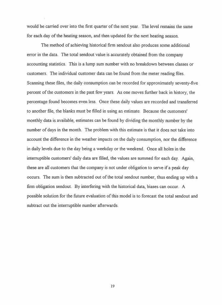
would be carried over into the first quarter of the next year. The level remains the same
for each day of the heating season, and then updated for the next heating season.
The method of achieving historical firm sendout also produces some additional
error in the data. The total sendout value is accurately obtained from the company
accounting statistics. This is a lump sum number with no breakdown between classes or
customers. The individual customer data can be found from the meter reading files.
Scanning these files, the daily consumption can be recorded for approximately seventy-five
percent of the customers in the past few years. As one moves further back in history, the
percentage found becomes even less. Once these daily values are recorded and transferred
to another file, the blanks must be filled in using an estimate. Because the customers'
monthly data is available, estimates can be found by dividing the monthly number by the
number of days in the month. The problem with this estimate is that it does not take into
account the difference in the weather impacts on the daily consumption, nor the difference
in daily levels due to the day being a weekday or the weekend. Once all holes in the
interruptible customers' daily data are filled, the values are summed for each day. Again,
these are all customers that the company is not under obligation to serve if a peak day
occurs. The sum is then subtracted out of the total sendout number, thus ending up with a
firm obligation sendout. By interfering with the historical data, biases can occur. A
possible solution for the future evaluation of this model is to forecast the total sendout and
subtract out the interruptible number afterwards.
19

EVALUATION OF MODEL RESULTS
The results of the equation estimated is as follows:
Firm Sendout =
-2840.87 * Current Day Wind-chill(30.374)
-1227.59 * Previous Day Wind-chill (16.353)
-8.5946 * Current Day Wind-chill Squared(3.5452)
+1.4036 * Real Disposable Income(8.9106)
+140654 (7.0106)
R Squared .8604R Bar Squared .8597F 4, 717 1105.21Durbin Watson 1.1221
All the coefficients turned out as expected, both in sign and in magnitude. For the
current day wind-chill, as these values becomes more extreme (more negative), then the
impact on firm sendout is an increase of about 2,841 MCF. This is a fairly representative
incremental change to be given to a one unit decrease in a negative wind-chill. As the
wind-chill becomes positive, this variable will begin to take away from the firm sendout
value. This is not of any concern for the model is to be used for peaking extreme negative
wind-chill values only. The coefficient for the previous day wind-chill allows for a 1,228
MCF increase in the firm sendout level when the previous day weather becomes more
extreme. This is a correct modeling of the buildup effect of a previous cold day. The
20
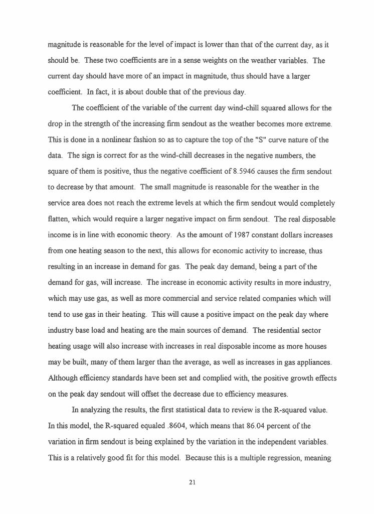
magnitude is reasonable for the level of impact is lower than that of the current day, as it
should be. These two coefficients are in a sense weights on the weather variables. The
current day should have more of an impact in magnitude, thus should have a larger
coefficient. In fact, it is about double that of the previous day.
The coefficient of the variable of the current day wind-chill squared allows for the
drop in the strength of the increasing firm sendout as the weather becomes more extreme.
This is done in a nonlinear fashion so as to capture the top of the "S" curve nature of the
data. The sign is correct for as the wind-chill decreases in the negative numbers, the
square of them is positive, thus the negative coefficient of 8.5946 causes the firm sendout
to decrease by that amount. The small magnitude is reasonable for the weather in the
service area does not reach the extreme levels at which the firm sendout would completely
flatten, which would require a larger negative impact on firm sendout. The real disposable
income is in line with economic theory. As the amount of 1987 constant dollars increases
from one heating season to the next, this allows for economic activity to increase, thus
resulting in an increase in demand for gas. The peak day demand, being a part of the
demand for gas, will increase. The increase in economic activity results in more industry,
which may use gas, as well as more commercial and service related companies which will
tend to use gas in their heating. This will cause a positive impact on the peak day where
industry base load and heating are the main sources of demand. The residential sector
heating usage will also increase with increases in real disposable income as more houses
may be built, many of them larger than the average, as well as increases in gas appliances.
Although efficiency standards have been set and complied with, the positive growth effects
on the peak day sendout will offset the decrease due to efficiency measures.
In analyzing the results, the first statistical data to review is the R-squared value.
In this model, the R-squared equaled .8604, which means that 86.04 percent of the
variation in firm sendout is being explained by the variation in the independent variables.
This is a relatively good fit for this model. Because this is a multiple regression, meaning
21

that it involves the use of several independent variables, it is worthwhile to evaluate the
adjusted R-squared to get a more accurate picture of the goodness of fit of the regression
line. The adjusted R-squared is developed from the R-squared, however, it penalizes for
the loss in degrees of freedom that occurs when more independent variables are added.
Resulting in an adjusted R-squared of .8597 means that 85.97 percent of the variation in
the firm sendout is being explained by the four independent variables. Again, this is a
good fit.
The next step is to test the individual statistical significance of each independent
variable in the model. The criteria used is a West for a ninety-five percent confidence
interval. The critical t-value from the t-distribution table is 1.645. The null hypothesis
tested is that each coefficient individually is equal to zero. If this null hypothesis cannot be
rejected, then the coefficient is said to be not statistically different from zero, thus there is
no basis for a relationship between the independent variable and the dependent variable.
Since this independent variable would lend no explanatory power to the model, it should
be dropped from the equation. The rejection of the null hypothesis says that the
coefficient is statistically different from zero, thus lends explanatory value to the model
and should remain in the equation. The rejection of the null hypothesis occurs when the
calculated t-values are greater than the critical t-value. Since all the calculated t-values are
all greater than the critical value, this allows for the rejection of all the null hypotheses.
All the variables are statistically significant and add explanatory value to the model and
should remain.
Using the F test can allow for testing if the model as a whole is statistically
significant. This is a joint hypothesis test of a null hypothesis that says all the coefficients
are equal to zero. This is tested against the alternative hypothesis that at least one of the
coefficients does not equal zero, meaning that it would have some explanatory power.
The rejection of the null hypothesis means that the model is better able to explain the
dependent variable than just using the mean of the dependent variable for predictive
22
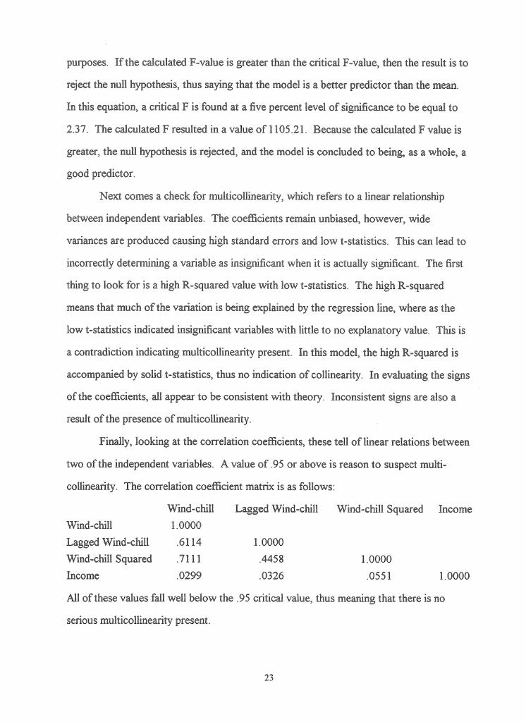
purposes. If the calculated F-value is greater than the critical F-value, then the result is to
reject the null hypothesis, thus saying that the model is a better predictor than the mean.
In this equation, a critical F is found at a five percent level of significance to be equal to
2.37. The calculated F resulted in a value of 1105.21. Because the calculated F value is
greater, the null hypothesis is rejected, and the model is concluded to being, as a whole, a
good predictor.
Next comes a check for multicollinearity, which refers to a linear relationship
between independent variables. The coefficients remain unbiased, however, wide
variances are produced causing high standard errors and low t-statistics. This can lead to
incorrectly determining a variable as insignificant when it is actually significant. The first
thing to look for is a high R-squared value with low t-statistics. The high R-squared
means that much of the variation is being explained by the regression line, where as the
low t-statistics indicated insignificant variables with little to no explanatory value. This is
a contradiction indicating multicollinearity present. In this model, the high R-squared is
accompanied by solid t-statistics, thus no indication of collinearity. In evaluating the signs
of the coefficients, all appear to be consistent with theory. Inconsistent signs are also a
result of the presence of multicollinearity.
Finally, looking at the correlation coefficients, these tell of linear relations between
two of the independent variables. A value of .95 or above is reason to suspect multi
collinearity. The correlation coefficient matrix is as follows:
Wind-chill Lagged Wind-chill Wind-chill Squared Income Wind-chill 1.0000Lagged Wind-chill .6114 1.0000Wind-chill Squared .7111 .4458 1.0000Income .0299 .0326 .0551 1.0000
All of these values fall well below the .95 critical value, thus meaning that there is no
serious multicollinearity present.
23

Because this data is strictly time series, the presence of serial correlation is most
probable. This occurs when the assumption that the correlation between the error terms is
zero is violated. There should not be any relationship between the errors from one period
to the next. Although the estimates are still unbiased and consistent, they are no longer
efficient. This causes the estimated variances to be smaller than the population variances,
thus the t-statistics are too large. Some variables will be falsely declared significant when
they really are insignificant. The most common method of detection is the use of the
Durbin-Watson statistic. This calculates how the error varies from one period to the next.
If there is no correlation over time, the Durbin-Watson statistic will converge to the value
of two. The Durbin-Watson test calculated for this model is 1.1221. At a five percent
level of significance with four independent variables, the lower Durbin-Watson value is
1.59 and the upper is 1.76. A calculated Durbin-Watson lower than 1.59 indicates the
presence of positive serial correlation The Cochrance-Orcutt procedure was used in an
attempt to correct the serial correlation. With this procedure, a series of iterations occur,
each of which produces a better estimate of rho than the previous one. This method could
not correct the serial correlation, even when lagged one period to fourteen periods, and
several combinations in-between.
Some causes of serial correlation were evaluated for insight on the problem. One
cause could be misspecification of the functional form. Many forms were attempted
ranging from straight linear to squaring the current and previous day wind chills to taking
the log of the two wind chills. All forms produced serial correlation that could not be
corrected. Another cause could be the omission of an important variable. The wind-chill
variables provide the necessary weather explanation, however, the economic variable of
real disposable income may not capture the entire effect of the economic activity on the
gas sendout. The impact not being captured is most likely the efficiency impacts due to
changes in the technology of appliances. Because this is the best service area economic
data available to give some sort of measurement for economic activity, it will remain in the
24

model. A linear time trend variable was attempted, but proved to be insignificant when
joining the equation already consisting of the real disposable income variable. Although
serial correlation creates problems, the model is theoretically sound and appears to be a
good predictor overall for the gas peak design day.
The final problem area to evaluate is the probable measurement error in the
dependent variable. This is a good possibility knowing that much estimation occurred in
subtracting the interruptible values out of the historical total sendout to reach historical
firm sendout values. The result is that if the errors are random, which in this case they are
likely to be, then the estimates are still unbiased. The t-statistics may tend to be smaller,
but since all the t-statistics were large enough to show significance, this measurement
error does not create any large statistical problems. Because this is the best method so far
in determining a historical firm sendout due to lack of good historical daily data for each
customer, a more accurate account cannot be made.
25

SUMMARY AND CONCLUSIONS
The design day forecast depends on using extreme weather conditions for the
design day parameters. The current day wind-chill is the second worst in thirty years,
calculated at -58. The previous day wind-chill chosen was the actual previous day to the
current day parameter, calculated at a value of -38.5. The real disposable income used for
the 1993/1994 heating season was 136,702 of 1987 dollars. Plugging these values into the
model produces a firm sendout of 515,654 MCF, or 530,092 DTH. This model remains
constant throughout the ten year forecast period, to be re-evaluated and updated each
year. The short term forecast of the next heating season is the most important purpose of
this model.
The actual peak for the 1993/1994 winter season occurred on January 18, 1994,
where firm sendout reached an all-time high of 513,876 MCF, or 528,261 DTH. The
temperature conditions were not as extreme as the design day parameters. The actual
wind-chill for January 18, 1994 was -55, and the previous day wind-chill was -25. The
forecasted firm sendout was approximately only one percent off, however, the weather
conditions were less extreme. Plugging in the actual January 18 weather conditions into
the estimated equation produces a predicted sendout of 493,468 MCF, or 507,285 DTH.
This gives a variation between forecast versus actual of -4.14 percent.
There are several areas for future assessment of this model. A first consideration is
to evaluate pre 1985 data. One possible way of doing this is to use an appropriate slope
change dummy variable. Another way is through the use of additional appropriate
independent variables which may reflect the structural changes that have occurred. A
second consideration is continued exploration of the utilization of similar economic data.
Some possibilities for other parameters are employment levels and gross product output.
26
A review of the procedure for estimating historical daily consumption of customers
migrating from the firm category is necessary. A possible solution would be to use total
sendout as the dependent variable, subtracting an interruptible value out of the forecasted
total sendout afterwards. This method would allow for the use of solid historical data,
reducing the measurement error, thus increasing the statistical validity of the model. This
also allows for the most current mix of interruptible customers to be analyzed and for a
revised interruptible number to be used each year. This should produce a more accurate
picture of the current status of the industry.
Another future assessment would be to run the model with omitting the warmer
days. A potential benefit would be a model which better captures the system's response to
the coldest days. This could also help to reduce the serial correlation. It is observed that
annual peaks have occurred on all days including weekdays, weekends, and holidays.
However, it is reasonable to expect that lifestyle, as reflected by day of the week, may
affect daily firm gas requirements. This could be reflected with the aid of dummy variables
for distinguishing the different days of the week.
A final future assessment would be to attempt separate regressions for each
heating season. The same form would be used, allowing the coefficients to change. This
approach would eliminate the need to capture the slow changes in economics,
demographics, appliance stacks and efficiencies, and prices over the historical period.
This model was filed in the previous year long term natural gas forecast and is
currently being used for forecasting in the utility's gas planning department. The
limitations of this model is that it is only a good predictor for the extreme weather
conditions, thus only should be used in evaluating the peak day. The future assessment of
this model is currently being evaluated and approved by management for any revisions and
updates.
27

BIBLIOGRAPHY
Bourcier, D. V.. Kazin, C. A.. "Utility Survey Results on Forecasting Methods and Assumptions." New England Power Planning.
Broehl, John H.. "An End-Use Approach to Demand Forecasting." SHAPES Users Seminar. San Antonio, Texas. July, 1991.
Cincinnati Gas and Electric Company. 1993 Natural Gas Long Term Forecast.Pages 1-60 - 1-65.
Electric Power Research Institute. Approaches to Load Forecasting: Proceedings of the Third EPRI Load Forecasting Symposium. Palo Alto, California. July, 1982.
Huss, William R.. "What Makes a Good Load Forecast?" Public Utility Fortnightly. November 28, 1985. Pages 27-35.
Little, John W.. Rosenbloom, Jeffeiy A.. "Bend-Over". Public Utility Fortnightly.April 1, 1994. Pages 20-23.
"Order 636: The Restructuring Rule." ENVOLVE. Volume 5. Number 4. Pages 1-5.
Pindyck, Robert S. Rubinfeld, Daniel L.. Econometric Models and Economic Forecasts. McGraw-Hill, Inc. 1981.
Vorys, Sater, Seymour and Pease. "Ohio Energy Report, Special Edition." April, 1992. Pages 1-4.
West Ohio Gas Company. 1993 Natural Gas Long Term Forecast. Page 47.
28
ENDNOTES
1 Vorys, Sater, Seymour and Pease. "Ohio Energy Report, Special Edition."2 "Order 636: The Restructuring Rule." ENVOLVE.3 Bourcier, D. V. Kazin, C. A. "Utility Survey Results on Forecasting Methods and Assumptions."4 Huss, William R. "What Makes a Good Load Forecast?"5 Huss, William R. "What Makes a Good Load Forecast?"6 Broehl, John H. "An End-Use Approach to Demand Forecasting."7 Huss, William R. "What Makes a Good Load Forecast?"8 Cincinnati Gas and Electric Company. 1993 Natural Gas Long Term Forecast.9 West Ohio Gas Company. 1993 Natural Gas Long Term Forecast.10 Little, John W. Rosenbloom, Jeffery A. "Bend-Over."11 Little, John W. Rosenbloom, Jeffery A. "Bend-Over."
29