Information Sciences 180 (2010) 3562–3571

Contents lists available at ScienceDirect

Information Sciences

journal homepage: www.elsevier .com/locate / ins

Garden of eden configurations for 2-D cellular automata with rule 2460 N

Irfan S�iap a, Hasan Akin b,*, Ferhat S�ah c

a Department of Mathematics, Arts and Science Faculty, Yıldız Technical University, Istanbul, Turkeyb Department of Mathematics, Education Faculty, Zirve University, Gaziantep, Turkeyc Department of Mathematics Engineering, Yıldız Technical University, Istanbul, Turkey

a r t i c l e i n f o

Article history:Received 8 April 2009Received in revised form 6 April 2010Accepted 27 May 2010

Keywords:Cellular automataGarden of EdenMatrix algebra

0020-0255/$ - see front matter � 2010 Elsevier Incdoi:10.1016/j.ins.2010.05.039

* Corresponding author. Tel.: +90 5423575825; faE-mail addresses: isiap@yildiz.edu.tr (I. S�iap), ha

a b s t r a c t

An important problem in cellular automata theory is the reversibility of a cellular autom-aton which is related to the existence of Garden of Eden configurations in cellular auto-mata. In this paper, we study new local rules for two-dimensional cellular automataover the ternary field Z3 (the set of integers modulo three) with some of their importantcharacteristics. We obtain necessary and sufficient conditions for the existence of Gardenof Eden configurations for two-dimensional ternary cellular automata. Also by makinguse of the matrix representation of two-dimensional cellular automata, we provide analgorithm to obtain the number of Garden of Eden configurations for two-dimensional cel-lular automata defined by rule 2460 N. We present an application of the reversible two-dimensional ternary cellular automata to cryptography.

� 2010 Elsevier Inc. All rights reserved.

1. Introduction

Cellular automata are discrete dynamical systems that exhibit a variety of dynamic behaviors, although they are formedby simple basic components. Cellular automata were first used for modelling various physical and biological processes, andin computer science. The concept of cellular automata was initiated in the early 1950’s by J. von Neumann and Stan Ulam.Von Neumann [32] showed that a cellular automaton (CA) can be universal. He devised CA, each cell of which has a statespace of 29 states, and showed that the devised CA can execute any computable operation. However, due to their complexity,von Neumann rules were never implemented on a computer. In the beginning of the eighties, Wolfram in [33] studied inmuch detail a family of simple one-dimensional (1-D) CA rules (known as famous Wolfram rules) and showed that eventhese simplest rules are capable of emulating complex behavior.

Due to various applications of cellular automata in many disciplines (e.g., mathematics, physics, computer science, chem-istry and so on) with different purposes (e.g., simulation of natural phenomena, pseudo-random number generation, imageprocessing, analysis of universal model of computations, cryptography). The study of CA has received remarkable attention inthe last few years [2,3,5,6,8,12,13,21,22]. Most of the work for CA is done for the one-dimensional case [17,18]. Lately, two-dimensional (2-D) CA has found applications in traffic modelling. For instance multi-valued (including ternary case) cellularautomaton models for traffic flow are proposed in [26]. A CA has also found applications in cryptography [7], for instancepretty recently multi state CA has been used in applications on Cryptography [24] and especially 2-D CA has been proposedfor multisecret sharing scheme for color images [4].

Das [12] has studied the characterization of 1-D CA by means of matrix algebra. Inokuchi and Sato [18] have investigatedthe behaviors of 1-D CA generated by the local rule 156. Recently, investigating the algebraic structure in order to interpret2-D CA has been of interest to the researchers. Some basic and precise mathematical models using matrix algebra built on

. All rights reserved.

x: +90 3422116677.sanakin69@gmail.com (H. Akin), fsah@yildiz.edu.tr (F. S�ah).

I. S�iap et al. / Information Sciences 180 (2010) 3562–3571 3563

the field GF (2) (Galois field with two elements or Z2) were reported for characterizing the behavior of 2-D nearest neigh-borhood linear CA with null and periodic boundary conditions [12,13,21,22]. Further, Khan et al. [21] developed an analyticaltool to study all the nearest neighborhood 2-D CA linear transformations. They proposed a new rule convention by dividing2-D linear CA and tried to study the characterization of that 2-D CA with respect to different rules.

There are configurations (states) that are unreachable or nonconstructible, in other words, no state will produce them bythe application of the evolution rules in cellular automata. These states are called Garden of Eden (GOE) configurations. Kari[20] has proved that the reversibility of a cellular automaton with dimension larger or equal to two is not decidable. In otherwords, due to its complexity, Kari has shown that the inverse of a given cellular automaton with higher dimension cannot befound by an algorithm in general. Further, Durand in [14] shows that the problem of finding the inverse of a 2-D cellularautomaton is a very difficult problem. Here, in this paper, we attack this problem for a particular 2-D cellular automaton withrule number 2460. If a cellular automaton does not posses any GOE configuration then it is reversible. Hence, determiningthe GOE configurations is an important problem in cellular automata theory. Adamatzky in [1] has proposed three differentapplications for GOE in cellular automata. Here we briefly mention these three applications. However the reader is encour-aged to refer to [1] for detailed discussions. In [1], the first application is given for neural nets where a cell has three statesrest (0), excited (+) and refractory (-). The second application of GOE problem is on agents where every cell is an agent whicheither holds one of two or three beliefs, or holds no beliefs at all. The third application is on population where each cell pre-sents a resource or two different species. Another application area of GOE problem is in cryptography. For instance in [15], aspecial software tool in CRIPTOCEL project was developed in order to select the cryptographic schemes based on CA that areoptimal for hardware implementation. This software accepts linear and 2-D cellular automata having variable dimensions.The main problem in cryptography is the existence of the inverse of applied cryptographic method. In [15], backward iter-ation of irreversible cellular automata is proposed as an effective encryption strategy. This method uses 2-D cellular auto-mata and the original message is the starting configuration. In this special cryptographic method again the reversibility ofa two-dimensional CA plays a crucial role which is equivalent to the existence of GOE configurations. Another applicationof GOE is a traffic modelling problem. Schadschneider and Schreckenberg in [27] investigate the allowed configurationsin the stationary state of a cellular automaton model for single-lane traffic. In parallel dynamics some states are shown tobe GOE which are responsible for the strong short-ranged correlations. The examples listed above is not a full list of appli-cations of GOE but we believe that it shows the importance of GOE in cellular automata theory. A further investigation ofGOE for 1-D CA is done in [5,6,8,9,17–19,25]. Recently, Ying et al. [34] have given a necessary and sufficient condition to en-sure that a given configuration is a GOE for 2-D CA over the field Z2. They have proposed some algorithms to determine thenumber of GOE.

As mentioned above the problem of irreversibility which is equivalent to the existence of GOE configurations in 2-D cel-lular automata is a difficult problem in general. Further, 2-D cellular automata with states more than two have found appli-cations in different areas recently. However, in the literature the algebraic structure of 2-D ternary cellular and its propertiesare not studied yet. Here, in this paper, we define new local rules over the field Z3 ¼ f0;1;2g for 2-D cellular automata. Weobtain a necessary and sufficient condition to determine whether a configuration is a GOE or not for 2-D CA generated by thelocal rule 2460 N. By making use of matrix algebra, we present an algorithm to compute the number of GOE configurationsfor a 2-D cellular automaton. Further, the Theorem 3.3 studies the existence of GOE which also tells whether a cellularautomaton is invertible or not. Finally, we discuss the applicability of our study, we present an application of the reversible2-D ternary cellular automata to cryptography.

2. Preliminaries

In this section, we give some basic definitions and we introduce 2-D CA over the field Z3 with respect to some local rules.We explore the representation of a ternary two-dimensional cellular automaton.

First, we recall the definition of a cellular automaton. For this, we consider the 2-dimensional integer lattice Z2 and theconfiguration space X ¼ f0;1;2gZ

2with elements

r : Z2 ! f0;1;2g:

The value of r at a point v 2 Z2 will be denoted by rv. Let u1; . . . ;us 2 Z2 be a finite set of distinct vectors and f:{0,1,2}s ? {0,1,2} be a function. A cellular automaton with local rule f is defined as a pair (X,Tf), where the global transitionmap Tf: X ? X is given by

ðTf rÞv ¼ f ðrvþu1 ; . . . ;rvþus Þ; where v 2 Z2:

The function f is called local rule and the space X is assumed to be equipped with a (metrizable) Tychonoff topology. For afixed v 2 Z2, let Uv: X ? X be the shift map: Uv(a) = bm, where bm = am�v, for all m 2 Z2. A cellular automaton is a continuousmap which commutes with all shifts. It is easily seen that the global transition map Tf introduced above and the shift oper-ator Uv are continuous in this topology (see [2,16] for the details).

The 2-D finite cellular automaton consists of m � n cells arranged in m rows and n columns, where each cell takes one ofthe values of 0, 1 or 2. A configuration of the system is an assignment of states to all the cells. Every configuration determinesa next configuration via a linear transition rule that is local in the sense that the state of a cell at time (t + 1) depends only on

3564 I. S�iap et al. / Information Sciences 180 (2010) 3562–3571

the states of some of its neighbors at time t using modulo 3. For 2-D CA nearest neighbors, there are nine cells arranged in a3 � 3 matrix centering that particular cell (see [10,12,13] for the details).

For 2-D CA there are some classic types of neighborhoods, but in this work only we restrict ourselves to the adjacentneighbors. So, we can define the (t + 1)th state of the (i, j)th cell as follows;

xðtþ1Þði;jÞ ¼ f xðtÞði;jÞ; x

ðtÞðiþ1;jÞ; x

ðtÞðiþ1;j�1Þ; x

ðtÞði;j�1Þ; x

ðtÞði�1;j�1Þ; x

ðtÞði�1;jÞ; x

ðtÞði�1;jþ1Þ; x

ðtÞði;jþ1Þ; x

ðtÞðiþ1;jþ1Þ

� �

¼ a0xðtÞði;jÞ þ a1xðtÞðiþ1;jÞ þ a2xðtÞðiþ1;j�1Þ þ a3xðtÞði;j�1Þ þ a4xðtÞði�1;j�1Þ þ a5xðtÞði�1;jÞ þ a6xðtÞði�1;jþ1Þ þ a7xðtÞði;jþ1Þ þ a8xðtÞðiþ1;jþ1Þðmod3Þ; ð2:1Þ

where a0; a1; . . . ; a8 2 Z3. The value of each cell for the next state may not depend upon all nine neighbors. The dependencewill be restricted to the case of being zero or nonzero, in other words if the coefficients in (2.1) equal to 1 or 2, then this casewill be assumed to be the same. This approach is adopted in this paper though these cases may be further distinguished. Inother words, the rule will depend on the cells addresses which are nonzero. The linear combination of the neighboring cellsthat are nonzero formulates the rule number of a 2-D cellular automaton over the field Z3: The conventional method of defin-ing a rule number for a linear rule in 2-D CA can be explained by Table 1 where xðk;hÞ 2 Z3.

The rule numbering depends on the addresses of nonzero cells governed by the Eq. (2.1). Under this assumption, a rulenumber of a CA will be a possible sum of the numbers in the set {30,31, . . . ,38}. For instance, if the dependency is on the cells31 and 32 as defined in Table 1, the rule is called Rule 31 + 32 = 12. As mentioned above, we do not define Rule 2 or any othernumber which is not a sum of possible combinations from the set {30,31, . . . ,38}. However, since a cellular automaton is addi-tive the sum of Rule 1 with itself already covers this case implicitly. For example, since 30 + 31 + � � � + 38 = 9840 Rule 9840means that the midpoint cell x(i, j) depends on all surrounding neighboring cells and itself. If central cell depends on the fourneighborhoods (top, right, bottom and left), it is called Rule 2460 (see Table 2). In brief, we do not distinguish between non-zero coefficients as having value 1 or 2. As it is defined above there are 29 rules altogether.

Regarding the neighborhood of the extreme cells, two approaches exist.

� A Periodic Boundary cellular automaton is obtained by extending the boundaries in such a way that the extreme cells areconnected to the copies of itself.� A Null Boundary cellular automaton is obtained by extending the boundaries in such a way that the extreme cells are

connected to 0-states.

The auxiliary matrices that play an important role in the representation matrix of a 2-D cellular automaton also consid-ered in several papers ([10,13,21,22] and [34]) are

T1 ¼0 1 00 0 10 0 0

0B@

1CA and T2 ¼

0 0 01 0 00 1 0

0B@

1CA:

Lemma 2.1 ([29,30]). The next state of all Primary rules (1,3,9,27,81,273,729,2187,6561) of a ternary 2-D cellular automatoncan be represented as follows:

Rule 1 : ½Xtþ1� ¼ a0½Xt �;Rule 3 : ½Xtþ1� ¼ a1½Xt �½T2�;Rule 9 : ½Xtþ1� ¼ a2½T1�½Xt�½T2�;Rule 27 : ½Xtþ1� ¼ a3½T1�½Xt �;

Table 1Null boundary condition in 2-D finite CA3 � 3.

0 0 0 0 00 x(i�1,j�1) x(i�1,j) x(i�1,j+1) 00 x(i,j�1) x(i,j) x(i,j+1) 00 x(i+1,j�1) x(i+1,j) x(i+1,j+1) 00 0 0 0 0

Table 2The rule 2460(=3 + 27 + 243 + 2187).

0 2187 0243 0 30 27 0

I. S�iap et al. / Information Sciences 180 (2010) 3562–3571 3565

Rule 81 : ½Xtþ1� ¼ a4½T1�½Xt �½T1�;Rule 243 : ½Xtþ1� ¼ a5½Xt�½T1�;Rule 729 : ½Xtþ1� ¼ a6½T2�½Xt �½T1�;Rule 2187 : ½Xtþ1� ¼ a7½T2�½Xt �;Rule 6561 : ½Xtþ1� ¼ a8½T2�½Xt �½T2�;

where ½Xt� ¼x11 x12 x13

x21 x22 x23

x31 x32 x33

0@

1A is the state of a cellular automaton at time t and [Xt+1] is the state of the cellular automaton at time

t + 1 and ai 2 Z�3 ¼ Z3 n f0g.In the sequel, for simplification, we assume that a1 = b,a3 = c, a5 = d and a7 ¼ aða; b; c; d 2 Z�3Þ. Now, we define a 2-D finite

cellular automaton T2460 : ZZ2

3 ! ZZ2

3 generated by the rule 2460.

ðT2460xÞðtÞði;jÞ ¼ f xðtÞði;jÞ; xðtÞðiþ1;jÞ; x

ðtÞðiþ1;j�1Þ; x

ðtÞði;j�1Þ; x

ðtÞði�1;j�1Þ; x

ðtÞði�1;jÞ; x

ðtÞði�1;jþ1Þ; x

ðtÞði;jþ1Þ; x

ðtÞðiþ1;jþ1Þ

� �

¼ cxðtÞðiþ1;jÞ þ dxðtÞði;j�1Þ þ axðtÞði�1;jÞ þ bxðtÞði;jþ1Þðmod3Þ ¼ yðtÞði;jÞ;

where yðtÞði;jÞ ¼ xðtþ1Þði;jÞ and ½i� 1; iþ 1� � ½j� 1; jþ 1� \ Z2.

In this paper, we will only consider the 2-D finite cellular automaton with Null Boundary condition (N). It is well knownthat these cellular automata are discrete dynamical systems formed by a finite two-dimensional array m � n composed byidentical objects called cells. In order to characterize the rule 2460 N, we can use the following auxiliary table which helps ondefining the rule 2460.

Since the rules are linear and Rule 2460 = Rule 3 + Rule 27 + Rule 243 + Rule 2187, the following lemma stated in [29] and[30] formulates the Rule 2460.

Lemma 2.2. The t + 1-state of a 2-D cellular automaton with Rule number 2460 can be represented by the sum of t-state matrices as

½Xtþ1� ¼ b½Xt�½T2� þ c½T1�½Xt � þ d½Xt�½T1� þ a½T2�½Xt�:

In order to study the properties of a 2-D cellular automaton, we introduce a map I, a vector isomorphism, to transfer the

problem from matrix representation to column representation of the states as follows: Let

I : Mm�nðZ3Þ ! Zmn3 :

I takes the tth state [Xt] which is in matrix form and transforms it to a column in the following way

x11 x12 � � � x1n

x21 x22 � � � x2n

..

. ...� � � ..

.

xm1 xm2 � � � xmn

0BBBB@

1CCCCA! x11; x12; . . . ; x1n; . . . ; xm1; . . . ; xmnð ÞT : ð2:2Þ

Therefore, the local rules will be assumed to act on Zmn3 rather than the matrix space Mm�nðZ3Þ:

The matrix

CðtÞ ¼xðtÞ11 � � � xðtÞ1n

..

. . .. ..

.

xðtÞm1 . . . xðtÞmn

0BB@

1CCA

is called a configuration of the 2-D finite CA at time t.Interpretation of Eq. (2.2) leads to

ðT2460NÞmn�mn

xðtÞ11

..

.

xðtÞ1n

..

.

xðtÞm1

..

.

xðtÞmn

0BBBBBBBBBBBBBBB@

1CCCCCCCCCCCCCCCA

¼

xðtþ1Þ11

..

.

xðtþ1Þ1n

..

.

xðtþ1Þm1

..

.

xðtþ1Þmn

0BBBBBBBBBBBBBBB@

1CCCCCCCCCCCCCCCA

;

3566 I. S�iap et al. / Information Sciences 180 (2010) 3562–3571

where xðtþ1Þij ¼ axðtÞði�1Þj þ bxðtÞiðjþ1Þ þ cxðtÞðiþ1Þj þ dxðtÞiðj�1Þðmod3Þ, i denotes the ith row of the matrix C(t) and j denotes the column of

the matrix C(t). For example, xðtþ1Þ22 ¼ axðtÞ12 þ bxðtÞ23 þ cxðtÞ32 þ dxðtÞ21ðmod3Þ.

Theorem 2.3. Let a; b; c; d 2 Z�3;m P 2 and n P 2. Let the map T2460N be generated by the null boundary rule 2460. Then, therepresentation matrix of T2460N from Zmn

3 to Zmn3 which takes the tth state [Xt] (as identified in (2.2)) to the (t + 1) – state [Xt+1] is

given by:

ðT2460NÞmn�mn ¼

S cI 0 � � � � � � 0 0aI S cI � � � � � � 0 00 aI S � � � � � � 0 0... ..

. ... ..

. ... ..

.

0 � � � � � � 0 aI S cI

0 0 � � � � � � 0 aI S

0BBBBBBBBB@

1CCCCCCCCCA

ð2:3Þ

where each submatrix is of order n � n, and

Sn�n ¼

0 b 0 0 � � � 0 0d 0 b 0 � � � 0 00 d 0 b � � � 0 0... ..

. ... ..

. ... ..

. ...

0 � � � � � � 0 d 0 b

0 0 � � � � � � 0 d 0

0BBBBBBBBB@

1CCCCCCCCCA

: ð2:4Þ

For the proof, the reader is referred to [29] and [30].

3. The Garden of Eden of 2-D finite CA with rule 2460 N

The configurations that are unreachable are called Garden of Eden (GOE). In other words, a configuration of a cellularautomaton that does not have predecessors is called GOE (see [34] for the details). As mentioned in introduction, computingthe GOE configurations of a cellular automaton is an important notion in cellular automata theory. This notion was intro-duced by Moore [25]. Recently, Ying et al.. [34] have computed the number of GOE configurations of a 2-D cellular automatonover the binary field Z2: We here use a similar extended approach for computing the number of GOE configurations over theternary field Z3: In this section, we determine the number of GOE configurations for 2-D CA defined by rule 2460 N. We ob-tain a necessary and sufficient condition to determine whether a configuration is a GOE or not for the 2-D CA given by Eq.(2.3).

A straightforward algebraic interpretation of the definition of a GOE is the following lemma.

Lemma 3.1. If a 2-D cellular automaton over the field Z3 is represented by T2460N, then the number of configurations B for whichthe corresponding equation T2460NX = B has no solution equals to jGOEj (number of GOE configurations).

We introduce a recurrence definition of a matrix polynomial Pm(S) that is going to be used in the following Theorem 3.3.

Definition 3.2. Let S be a square matrix. Then the polynomial Pm(S) is defined as follows:

P�1ðSÞ ¼ 0; P0ðSÞ ¼ cI; PmðSÞ ¼ 2cSPm�1ðSÞ þ 2acPm�2ðSÞ; form P 1:

In this paper, the main result is the following Theorem.

Theorem 3.3. Let CAm�n be a 2-D cellular automaton with the rule 2460 N and B be a configuration of it. The configuration B is aGOE of CAm�n if and only if the rank of (Pm(S),K) is not equal to the rank of Pm(S), where K ¼

Pmi¼1Pm�iðSÞBi. Further, let P and Q be

two invertible matrices such that PPm(S)Q is a diagonal matrix of the following form:

D ¼ ðdijÞ ¼

1. .

.

10

. ..

0

0BBBBBBBBBB@

1CCCCCCCCCCA

: ð3:1Þ

If the column matrix PK has an entry ‘i1 for i P f different than zero, where f = max{ijdii – 0}, then, B is a GOE of CAm�n.

I. S�iap et al. / Information Sciences 180 (2010) 3562–3571 3567

Proof. Clearly, the augmented matrix of TX = Bmn�1 is

G ¼

S cI 0 0 0 � � � � � � 0 0 B1

aI S cI 0 0 � � � � � � 0 0 B2

0 aI S cI 0 � � � � � � 0 0 B3

0 0 aI S cI 0 � � � � � � 0 B4

..

. ... ..

. ... ..

. ... ..

. ... ..

. ...

0 0 � � � � � � � � � 0 aI S cI Bm�1

0 0 0 � � � � � � 0 0 aI S Bm

0BBBBBBBBBBBB@

1CCCCCCCCCCCCA

:

We define an auxiliary matrix A as follows:

A ¼

cI 0 0 � � � � � � 0S cI 0 0 � � � 0aI S cI 0 � � � 00 aI S cI � � � 0... ..

. ... ..

. ... ..

.

0 0 0 aI S cI

0BBBBBBBBB@

1CCCCCCCCCAðm�1Þn�ðm�1Þn

:

Then, the inverse of the matrix A is

A�1 ¼

cI 0 0 0 � � � 02S cI 0 0 � � � 0

cS2 þ 2aI 2S cI 0 � � � 02S3 þ 2acS cS2 þ 2aI 2S cI � � � 0

cS4 þ cI 2S3 þ 2acS cS2 þ 2aI 2S � � � 0

..

. ... ..

. ... ..

.0

Pm�2ðSÞ Pm�3ðSÞ Pm�4ðSÞ Pm�5ðSÞ � � � P0ðSÞ ¼ cI

0BBBBBBBBBBBB@

1CCCCCCCCCCCCAðm�1Þn�ðm�1Þn

:

Now we multiply the augmented matrix of TX = Bmn�1 by

H ¼

0 � � � 0 cI

0

A�1 ...

0

0BBBB@

1CCCCA

mn�mn

from the left. Next, we get

H � G ¼

0 � � � � � � � � � cI

0...

A�1 ...

..

.

0

0BBBBBBBBBB@

1CCCCCCCCCCA

mn�mn

�

S B1

aI B2

0 A B3

0 B4

..

. ...

0 Bm�1

0 0 � � � 0 aI S Bm

0BBBBBBBBBBBB@

1CCCCCCCCCCCCA

mn�ðmnþ1Þ

¼

0 0 0 0 � � � acI cS cBm

cS I 0 0 � � � 0 0 cB1

2S2 þ acI 0 I 0 � � � 0 0 2SB1 þ cB2

cS3 þ aS 0 0 I � � � 0 0ðcS2 þ 2aIÞB1

þ2SB2 þ cB3

..

. ... ..

. ... ..

. ... ..

. ...

SPm�2ðSÞ þ aPm�3ðSÞ 0 0 0 � � � 0 I

Pm�2ðSÞB1þPm�3ðSÞB2þ

� � � þ P1ðSÞBm�2þP0ðSÞBm�1

0BBBBBBBBBBBBBBBBBBB@

1CCCCCCCCCCCCCCCCCCCA

:

3568 I. S�iap et al. / Information Sciences 180 (2010) 3562–3571

By applying elementary row operations (taking appropriate multiples of the last and successive rows and adding them tothe first row) to the above matrix, we have

¼

2cS2Pm�2ðSÞþacSPm�3ðSÞþ

2cPm�4ðSÞ0 0 0 0 � � � 0 0 K

cS I 0 0 0 � � � 0 0 cB1

2S2 þ acI 0 I 0 0 � � � 0 0 2SB1 þ cB2

cS3 þ aS 0 0 I 0 � � � 0 0ðcS2 þ 2aIÞB1þ

2SB2 þ cB3

2S4 þ 2I 0 0 0 I � � � 0 0ð2S3 þ 2acSÞB1þ

ðcS2 þ 2aIÞB2 þ 2SB3 þ cB4

..

. ... ..

. ... ..

. ... ..

. ... ..

.

SPm�2ðSÞþaPm�3ðSÞ

0 0 0 0 � � � 0 IPm�2ðSÞB1 þ Pm�3ðSÞB2

þ � � � þ P1ðSÞBm�2 þ P0ðSÞBm�1

0BBBBBBBBBBBBBBBBBBBBBBBBB@

1CCCCCCCCCCCCCCCCCCCCCCCCCA

;

where K ¼Pm

i¼1Pm�iðSÞBi:

Now, by applying elementary column operations (multiplying the second, third, etc. columns with appropriate multiplesand adding them to the last column respectively) to the above matrix and also multiplying the first column by 2c, we have

S2Pm�2ðSÞþ2aSPm�3ðSÞþ

Pm�4ðSÞ0 0 0 0 � � � 0 0 K

2S I 0 0 0 � � � 0 0 0cS2 þ 2aI 0 I 0 0 � � � 0 0 0

2S3 þ 2acS 0 0 I 0 � � � 0 0 0cS4 þ cI 0 0 0 I � � � 0 0 0

..

. ... ..

. ... ..

. ... ..

. ... ..

.

2cSPm�2ðSÞ þ 2acPm�3ðSÞ 0 0 0 0 � � � 0 I 0

0BBBBBBBBBBBBBBBBB@

1CCCCCCCCCCCCCCCCCA

:

Hence, we have

M ¼

PmðSÞ 0 0 0 0 � � � 0 0 K

P1ðSÞ I 0 0 0 � � � 0 0 0P2ðSÞ 0 I 0 0 � � � 0 0 0P3ðSÞ 0 0 I 0 � � � 0 0 0P4ðSÞ 0 0 0 I � � � 0 0 0

..

. ... ..

. ... ..

. ... ..

. ... ..

.

Pm�1ðSÞ 0 0 0 0 � � � 0 I 0

0BBBBBBBBBBBB@

1CCCCCCCCCCCCA

:

If P and Q are invertible matrices such that PPm(S)Q is equal to a diagonal matrix as in (3.1), then we have

P 0 0 � � � 00 I 0 � � � 00 0 I � � � 0... ..

. ... ..

. ...

0 0 0 � � � I

0BBBBBB@

1CCCCCCAðmnÞ�ðmnÞ

�M �

Q 0 0 � � � 00 I 0 � � � 00 0 I � � � 0... ..

. ... ..

. ...

0 0 0 � � � I

0BBBBBB@

1CCCCCCAðmnþ1Þ�ðmnþ1Þ

¼

PPmðSÞ 0 0 � � � 0 PK

P1ðSÞ I 0 � � � 0 0P2ðSÞ 0 I � � � 0 0P3ðSÞ 0 0 � � � 0 0P4ðSÞ 0 0 � � � 0 0

..

. ... ..

. ... ..

. ...

Pm�1ðSÞ 0 0 � � � I 0

0BBBBBBBBBBBB@

1CCCCCCCCCCCCAðmnÞ�ðmnþ1Þ

�

Q 0 0 0 � � � 00 I 0 0 � � � 00 0 I 0 � � � 00 0 0 I � � � 0... ..

. ... ..

. ...

00 0 0 0 � � � I

0BBBBBBBBB@

1CCCCCCCCCAðmnþ1Þ�ðmnþ1Þ

I. S�iap et al. / Information Sciences 180 (2010) 3562–3571 3569

¼

PPmðSÞQ 0 0 0 0 � � � 0 PK

P1ðSÞQ I 0 0 0 � � � 0 0P2ðSÞQ 0 I 0 0 � � � 0 0P3ðSÞQ 0 0 I 0 � � � 0 0P4ðSÞQ 0 0 0 I � � � 0 0

..

. ... ..

. ... ..

. ... ..

. ...

Pm�1ðSÞQ 0 0 0 0 � � � I 0

0BBBBBBBBBBBB@

1CCCCCCCCCCCCA

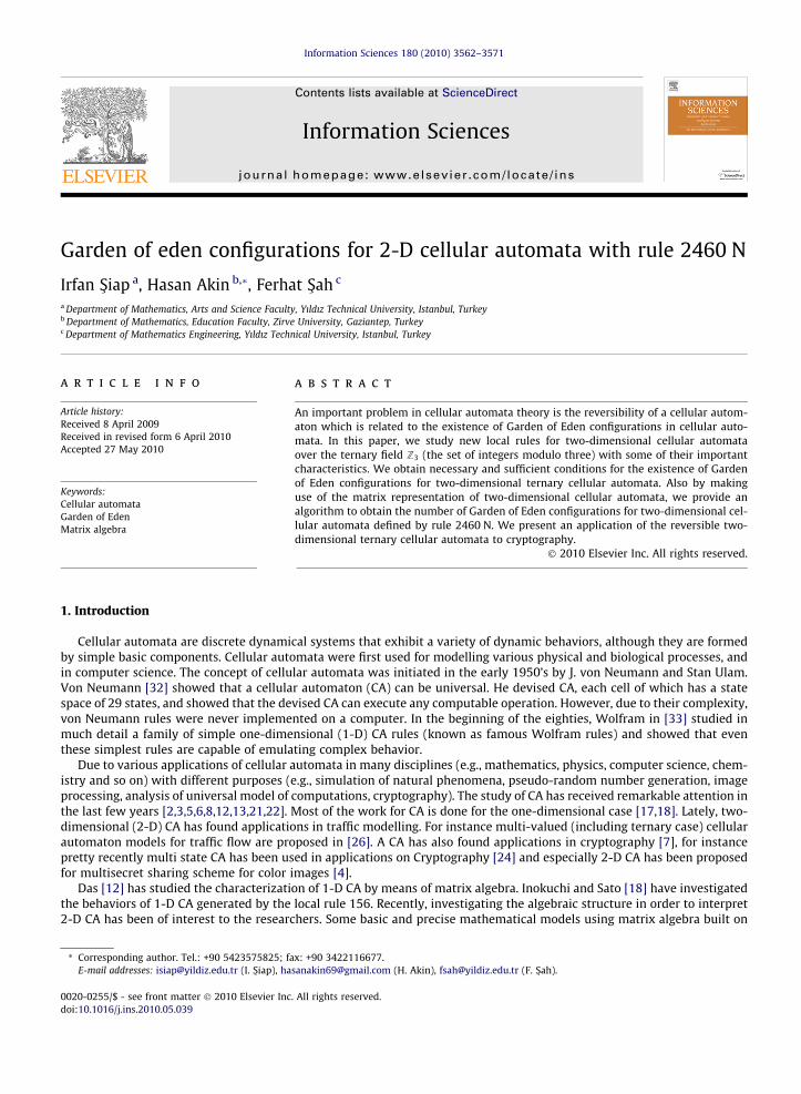
¼ ðT 0;B0Þ:

Let f = max{ijdii – 0}. It is clear that if there exists i P f such that ‘i – 0, then (PPm(S)Q = D,PK = L) does not have a solution,

where L ¼

‘1

‘2

..

.

‘n

0BBB@

1CCCA: h

Remark 3.4. Though our work is inspired by Ying and et al.’s paper [34] which considers the binary field case, we end upwith a slightly different method for determining the number of GOE configurations. This method avoids calculations for eachparticular case.

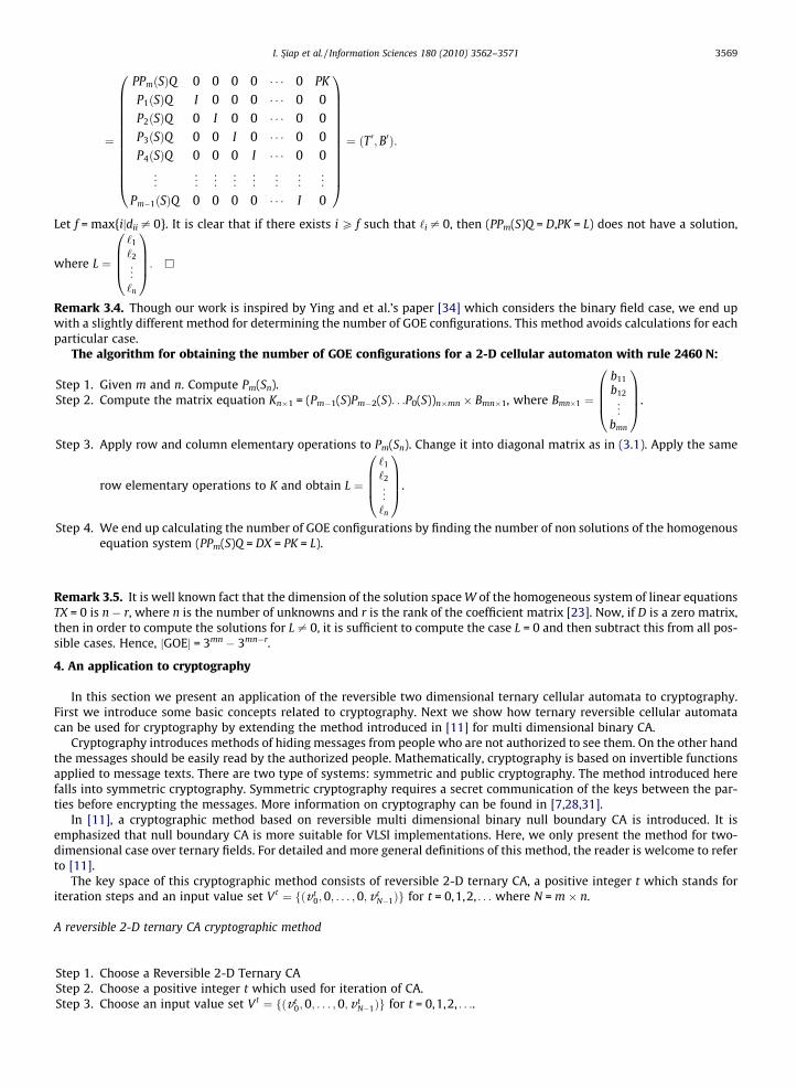
The algorithm for obtaining the number of GOE configurations for a 2-D cellular automaton with rule 2460 N:

Step 1. Given m and n. Compute Pm(Sn).b11

b12

0B

1C

Step 2. Compute the matrix equation Kn�1 = (Pm�1(S)Pm�2(S). . .P0(S))n�mn � Bmn�1, where Bmn�1 ¼ ...

bmn

BB@CCA.

Step 3. Apply row and column elementary operations to Pm(Sn). Change it into diagonal matrix as in (3.1). Apply the same

row elementary operations to K and obtain L ¼

‘1

‘2

..

.

‘n

0BBB@

1CCCA.

Step 4. We end up calculating the number of GOE configurations by finding the number of non solutions of the homogenousequation system (PPm(S)Q = DX = PK = L).

Remark 3.5. It is well known fact that the dimension of the solution space W of the homogeneous system of linear equationsTX = 0 is n � r, where n is the number of unknowns and r is the rank of the coefficient matrix [23]. Now, if D is a zero matrix,then in order to compute the solutions for L – 0, it is sufficient to compute the case L = 0 and then subtract this from all pos-sible cases. Hence, jGOEj = 3mn � 3mn�r.

4. An application to cryptography

In this section we present an application of the reversible two dimensional ternary cellular automata to cryptography.First we introduce some basic concepts related to cryptography. Next we show how ternary reversible cellular automatacan be used for cryptography by extending the method introduced in [11] for multi dimensional binary CA.

Cryptography introduces methods of hiding messages from people who are not authorized to see them. On the other handthe messages should be easily read by the authorized people. Mathematically, cryptography is based on invertible functionsapplied to message texts. There are two type of systems: symmetric and public cryptography. The method introduced herefalls into symmetric cryptography. Symmetric cryptography requires a secret communication of the keys between the par-ties before encrypting the messages. More information on cryptography can be found in [7,28,31].

In [11], a cryptographic method based on reversible multi dimensional binary null boundary CA is introduced. It isemphasized that null boundary CA is more suitable for VLSI implementations. Here, we only present the method for two-dimensional case over ternary fields. For detailed and more general definitions of this method, the reader is welcome to referto [11].

The key space of this cryptographic method consists of reversible 2-D ternary CA, a positive integer t which stands foriteration steps and an input value set Vt ¼ fðv t

0;0; . . . ;0;v tN�1Þg for t = 0,1,2, . . . where N = m � n.

A reversible 2-D ternary CA cryptographic method

Step 1. Choose a Reversible 2-D Ternary CAStep 2. Choose a positive integer t which used for iteration of CA.Step 3. Choose an input value set Vt ¼ fðv t

0;0; . . . ;0;v tN�1Þg for t = 0,1,2, . . ..

3570 I. S�iap et al. / Information Sciences 180 (2010) 3562–3571

Step 4. To encrypt the message (plain text) X0 apply the reversible 2-D ternary CA represented by T, by cooperating the inputset Vtt times and obtain to cipher text Xt in the following way

Xt ¼ TtX0 þXt�1

j¼0

Tt�j�1Vj:

P.S. The decryption method is a reversed process of encryption which is possible since T is invertible.Now, in order to illustrate the method we pick a moderate sized 2-D ternary CA with rule 2460 N studied in this paper.

We take m = 3 and n = 3, and first we compute the number of GOE configurations for a 2-D cellular automaton with rule

2460N and then we determine the reversibility of this CA. Let a = 2, b = 2, c = 2 and d = 1. Then, S ¼0 2 01 0 20 1 0

0@

1A. Next, we

apply the algorithm for determining the reversibility of this CA as follows:

Step 1. First, by applying the recurrence relations, we find P3(S) = S.Step 2.

P2ðSÞP1ðSÞ P0ðSÞð Þ ¼2 0 2 0 1 0 2 0 00 0 0 2 0 1 0 2 02 0 2 0 2 0 0 0 2

0B@

1CA

Step 3. Since P3(S) is not in diagonal form we need to find the invertible matrices P and Q such that PP3(S)Q is diagonal. If we

take P ¼0 1 00 0 11 0 1

0@

1A and Q ¼

1 0 10 1 00 0 1

0@

1A then, we have D ¼ PP3ðSÞQ ¼

1 0 00 1 00 0 0

0@

1A: Thus, L ¼ PK ¼

P P2ðSÞ P1ðSÞ P0ðSÞð ÞB ¼0 0 0 0 2 0 2 0 10 0 0 2 0 1 0 2 00 0 0 0 0 0 0 0 0

0@

1A � B ¼

‘1

‘2

‘3

0@

1A

3�1

¼2b5 þ 2b7 þ b9

2b4 þ b6 þ 2b8

0

0@

1A.

Step 4. It is clear that the rank (P(P2(S)P1(S)P0(S))) = r = 2.

Since the homogenous equation system PPm(S)Q = DX = PK = L is consistent, there is no GOE. So, jGOEj = 0. In other words,this particular CA is reversible.

Now, we use this particular CA for the cryptographic method:

Step 1. Choose T ¼S 2I 02I S 2I0 2I S

0@

1A.

Step 2. Choose a positive integer 4 which used for iteration of CA.Step 3. We choose an input value set Vt = {(t,0, . . .,0,2 + 2t)} for t = 0,1,2,3,4. . . modulo 3.Step 4. To encrypt the message (plain text) X0 = [1,2,0,0,2,2,1,2,1]T apply the reversible 2-D ternary CA represented by T,

by cooperating the input set Vt, and obtain to cipher text X5 in the following way

X5 ¼ T5X0 þX4

j¼0

T4�jV j:

So, the encrypted message becomes

X5 ¼ ½0;0;2;0;2;1;1;2;2�T :

In order to have a good secrecy the size of the key space is crucial. In binary case [11], it is shown that this method isbetter than some other approaches of cryptography. In this section an illustrative example is presented, though cellular auto-mata applications in cryptography are still evaluated.

5. Conclusion

Some results for 2-D binary cellular automaton have been generalized to the ternary case. Some properties of 2-D ternarycellular automaton have been presented and studied. Especially, this paper focuses on necessary and sufficient conditions forthe existence of GOE configurations for 2-D ternary cellular automaton defined by the rule number 2460 N. Also, an algo-rithm has been presented for computing the number of GOE configurations. Further properties of 2-D CA over ternary orother fields remain to be of great future research interest.

I. S�iap et al. / Information Sciences 180 (2010) 3562–3571 3571

Acknowledgements

The authors thank the anonymous referees for their careful reading and useful comments which greatly improved thewriting and presentation of the paper. Also, the authors would like to thank the editor(s) for their valuable points while edit-ing the final version of the paper.

References

[1] A. Adamatzky, Nonconstructible blocks in 1D cellular automata: minimal generators and natural systems, Appl. Math. Comput. 99 (1999) 77–91.[2] H. Akın, On the directional entropy of Z2 – actions generated by additive cellular automata, Appl. Math. Computation 170 (1) (2005) 339–346.[3] H. Akın, I. Siap, On cellular automata over Galois rings, Inform. Process. Lett. 103 (1) (2007) 24–27.[4] G. Alvarez, L. Hernandez Encinas, A. Martin del Rey, A multisecret sharing scheme for color images based on cellular automata, Inform. Sci. 178 (2008)

4382–4395.[5] S. Amoroso, G. Cooper, The Garden-of-Eden theorem for finite configurations, Proc. Amer. Math. Soc. 26 (1970) 158–164.[6] S. Amoroso, G. Cooper, Y.N. Patt, Some clarification of the concept of a Garden-of-Eden configuration, J. Comput. System Sci. 10 (1975) 77–82.[7] S.R. Blackburn, S. Murphy, K.G. Peterson, Comments on theory and applications of cellular automata in cryptography, IEEE Trans. Comput. 46 (1997)

637–638.[8] H. Brian, S. James, A Exact Enumeration of Garden of Eden partitions, Comb. Num. Th., de Gruyter, Berlin, 2007 (pp. 299-303).[9] L.K. Bruckner, On the Garden-of-Eden problem for one-dimensional cellular automata, Acta Cybernetica 4 (3) (1979) 259–262.

[10] P. Chattopdhyay, P.P. Choudhury, K. Dihidar, Characterisation of a particular hybrid transformation of two-dimensional cellular automata, Comput.Math. Appl. 38 (1999) 207–216.

[11] Z. Chuanwu, P. Qicong, L. Yubo, Encryption based on reversible cellular automata, Communications, circuits and systems and West Sino expositions, in:IEEE 2002 International Conference 2, 2002, pp. 1223–1226.

[12] A.K. Das, Additive cellular automata: theory and application as a built-in self-test structure, Ph.D. Thesis, I.I.T. Kharagpur, India, 1990.[13] K. Dihidar, P.P. Choudhury, Matrix algebraic formulae concerning some exceptional rules of two dimensional cellular automata, Inform. Sci. 165 (2004)

91–101.[14] B. Durand, Inversion of 2D cellular automata: some complexity results, Theoret. Comput. Sci. 134 (1994) 387–401.[15] E. Franti, S. Goschin, M. Dascalu, N. Catrina, M. Dobrin, CRIPTOCEL: design of cellular automata based cipher schemes, Commun. Circ. Syst. 2 (2004)

1103–1107.[16] G.A. Hedlund, Endomorphisms and automorphisms of full shift dynamical system, Math. Syst. Th. 3 (1969) 320–375.[17] S. Inokuchi, On behaviors of cellular automata with rule 156, Bull. Inform. Cybernet. 30 (1) (1998) 121–131.[18] S. Inokuchi, T. Sato, On limit cycles and transient lengths of cellular automata with threshold rules, Bull. Inform. Cybernet. 32 (1) (2000) 23–60.[19] C. Jadur, J. Yazlle, On the dynamics of cellular automata induced from a prefix code, Adv. Appl. Math. 38 (2007) 27–53.[20] J. Kari, Reversibility of 2D cellular automata is undecidable, Physica D 45 (1990) 386–395.[21] A.R. Khan, P.P. Choudhury, K. Dihidar, S. Mitra, P. Sarkar, VLSI architecture of a cellular automata, Comput. Math. Appl. 33 (1997) 79–94.[22] A.R. Khan, P.P. Choudhury, K. Dihidar, R. Verma, Text compression using two dimensional cellular automata, Comput. Math. Appl. 37 (1999) 115–127.[23] S. Lipschutz, Theory and Problems of Linear Algebra, Mc Graw Hill Inc., 1990.[24] M. Mihaljevic, Y. Zheng, H. Imai, A family of fast dedicated one-way hash functions based on linear cellular automata over GF(q), IEICE Trans. Fundam.

E82-A (1999) 40–47.[25] E.F. Moore, Machine models of self-reproduction, Proc.1 Symp. Appl. Math. 14 (1962) 1733.[26] K. Nishinar, D. Takahashi, Multi-value cellular automaton models and metastable states in a congested phase, J. Phys. A: Math. Gen. 33 (2000) 7709–

7720.[27] A. Schadschneider, M. Schreckenberg, Garden of Eden states in traffic models, J. Phys. A: Math. Gen. 31 (1998) 225–231.[28] B. Schneier, Applied Cryptography, second ed., John Wiley & Sons, 2002.[29] I. Siap, H. Akın, F. Sah, Characterization of two dimensional cellular automata over ternary fields, in: ICSM0’09 Proceedings, 20–22 January 2009, pp.

22–24.[30] I. Siap, H. Akın, F. Sah, Characterization of two dimensional cellular automata over ternary fields, Journal Of The Franklin Institute. doi:10.1016/

j.jfranklin.2010.02.002.[31] D.R. Stinson, Cryptography Theory and Practice, CRC Press, Inc., 2002.[32] J. Von Neumann, The theory of self-reproducing automata, in: A.W. Burks (Ed.), Univ. of Illinois Press, Urbana, 1966.[33] S. Wolfram, Statistical mechanics of cellular automata, Rev. Mod. Phys. 55 (3) (1983) 601–644.[34] Z. Ying, Y. Zhong, D. Pei-min, On behavior of two-dimensional cellular automata with an exceptional rule, Inform. Sci. 179 (5) (2009) 613–622.