GAMS/MINOS MINOS 1

GAMS/MINOS

Table of Contents:

.....................................................................................................................................1. INTRODUCTION.............................................................................................. 22. HOW TO RUN A MODEL WITH GAMS/MINOS.......................................... 23. OVERVIEW OF GAMS/MINOS...................................................................... 2

3.1. Linear programming .................................................................................... 33.2. Problems with a Nonlinear Objective .......................................................... 43.3. Problems with Nonlinear Constraints .......................................................... 6

4. GAMS OPTIONS .............................................................................................. 74.1. Options specified through the option statement........................................... 74.2. Options specified through model suffixes ................................................... 8

5. SUMMARY OF MINOS OPTIONS ................................................................. 85.1. Output related options.................................................................................. 85.2. Options affecting Tolerances ....................................................................... 95.3. Options affecting Iteration limits ................................................................. 95.4. Other algorithmic options ............................................................................ 95.5. Examples of GAMS/MINOS option file ................................................... 10

6. Special Notes.................................................................................................... 116.1. Modeling Hints .......................................................................................... 116.2. Storage ....................................................................................................... 11

7. The GAMS/MINOS Log File........................................................................... 127.1. Linear Programs......................................................................................... 127.2. Nonlinear Objective ................................................................................... 157.3. Nonlinear constraints ................................................................................. 17

8. Detailed Description of MINOS Options......................................................... 199. Acknowledgements .......................................................................................... 3910. References ...................................................................................................... 40

2 MINOS GAMS/MINOS

1. INTRODUCTION

This section describes the GAMS interface to MINOS which is a general purposenonlinear programming solver. GAMS/MINOS is a specially adapted version of the solverthat is used for solving linear and nonlinear programming problems.

GAMS/MINOS is designed to find solutions that are locally optimal. The nonlinearfunctions in a problem must be smooth (i.e., their first derivatives must exist). Thefunctions need not be separable. Integer restrictions cannot be imposed directly.

A certain region is defined by the linear constraints in a problem and by the bounds on thevariables. If the nonlinear objective and constraint functions are convex within this region,any optimal solution obtained will be a global optimum. Otherwise there may be severallocal optima, and some of these may not be global. In such cases the chances of finding aglobal optimum are usually increased by choosing a staring point that is “sufficientlyclose,” but there is no general procedure for determining what “close” means, or forverifying that a given local optimum is indeed global.

GAMS allows you to specify values for many parameters that control GAMS/MINOS, andwith careful experimentation you may be able to influence the solution process in a helpfulway. All MINOS options available through GAMS/MINOS are summarized at the end ofthis chapter.

2. HOW TO RUN A MODEL WITH GAMS/MINOS

MINOS is capable of solving models of the following types: LP, NLP and RMINLP. IfMINOS is not specified as the default LP, NLP or RMINLP solver, then the followingstatement can be used in your GAMS model:

option lp=minos5; { or nlp or rminlp }

It should appear before the solve statement.

3. OVERVIEW OF GAMS/MINOS

GAMS/MINOS is a system designed to solve large-scale optimization problems expressedin the following form:

Minimize F(x) + cT x + dT y (1)subject to f(x) + A1 y <> b1 (2)

A2 x + A3 y <> b2 (3)l ≤ x,y ≤ u (4)

GAMS/MINOS MINOS 3

where the vectors c, d, b1, b2, l, u and the matrices A1, A2, A3 are constant, F(x) is a smoothscalar function, and f(x) is a vector of smooth functions. The < > signs mean thatindividual constraints may be defined using ≤, = or ≥ corresponding to the GAMSconstructs =L= , =E= and =G=.

The components of x are called the nonlinear variables, and the components of y are thelinear variables. Similarly, the equations in (2) are called the nonlinear constraints, and theequations in (3) are the linear constraints. Equations (2) and (3) together are called thegeneral constraints.

Let m1 and n1 denote the number of nonlinear constraints and variables, and let m and ndenote the total number of (general) constraints and variables. Thus, A3 has m-m1 rows andn-n1 columns.

The constraints (4) specify upper and lower bounds on all variables. These arefundamental to many problem formulations and are treated specially by the solutionalgorithms in GAMS/MINOS. Some of the components of l and u may be -∞ or +∞respectively, in accordance with the GAMS use of -INF and + INF.

The vectors b1 and b2 are called the right-hand side, and together are denoted by b.

3.1. Linear programming

If the functions F(x) and f(x) are absent, the problem becomes a linear program. Sincethere is no need to distinguish between linear and nonlinear variables, we use x rather thany. GAMS/MINOS converts all general constraints into equalities, and the only remaininginequalities are simple bounds on the variables. Thus, we write linear programs in the form

minimize cTxsubject to Ax + Is = 0

l ≤ x, s ≤ u

where the elements of x are your own GAMS variables, and s is a set of slack variables:one for each general constraint. For computational reasons, the right-hand side b isincorporated into the bounds on s.

In the expression Ax + Is = 0 we write the identity matrix explicitly if we are concernedwith columns of the associated matrix (AI). Otherwise we will use the equivalent notationAx + s = 0.

GAMS/MINOS solves linear programs using a reliable implementation of the primalsimplex method (Dantzig, 1963), in which the constraints Ax + Is = 0 are partitioned intothe form

BxB + NxN = 0,

4 MINOS GAMS/MINOS

where the basis matrix B is square and nonsingular. The elements of xB and xN are calledthe basic or nonbasic variables respectively. Together they are a permutation of the vector(x, s).

Normally, each nonbasic variable is equal to one of its bounds, and the basic variables takeon whatever values are needed to satisfy the general constraints. (The basic variables maybe computed by solving the linear equation BxB = NxN.) It can be shown that if an optimalsolution to a linear program exists, then it has this form.

The simplex method reaches such a solution by performing a sequence of iterations, inwhich one column of B is replaced by one column of N(and vice versa), until no suchinterchange can be found that will reduce the value of cTx.

As indicated nonbasic variables usually satisfy their upper and lower bounds. If anycomponents of xB lie significantly outside their bounds, we say that the current point isinfeasible. In this case, the simplex method uses a Phase 1 procedure to reduce the sum ofinfeasibilities to zero. This is similar to the subsequent Phase 2 procedure that optimizesthe true objective function cTx.

If the solution procedures are interrupted, some of the nonbasic variables may lie strictlybetween their bounds” lj < xj < uj. In addition, at a “feasible” or “optimal” solution, someof the basic variables may lie slightly outside their bounds: lj - δ < xj < lj or uj < xj + δwhere δ is a feasibility tolerance (typically 10-6). In rare cases, even a new nonbasicvariables might lie outside their bounds by as much as δ.

GAMS/MINOS maintains a sparse LU factorization of the basis matrix B , using aMarkowitz ordering scheme and Bartels-Golub updates, as implemented in the Fortranpackage LUSOL(Gill et al. 1987).(see Bartels and Golub, 1969; Bartels, 1971; Reid, 1976and 1982.) The basis factorization is central to the efficient handling of sparse linear andnonlinear constraints.

3.2. Problems with a Nonlinear Objective

When nonlinearities are confined to the term F(x) in the objective function, the problem isa linearly constrained nonlinear program. GAMS/MINOS solves such problems using areduced-gradient algorithm (Wolfe, 1962) combined with a quasi-Newton algorithmfollows that described in Murtagh and Saunders (1978).

In the reduced-gradient method, the constraints Ax + Is = 0 are partitioned into the form

BxB + SxS + NxN = 0

where xs is a set of superbasic variables. At a solution, the basic and superbasic variableswill lie somewhere between their bounds (to within the feasibility tolerance δ ) , whilenonbasic variables will normally be equal to one of their bounds, as before. Let thenumber of superbasic variables be s, the number of columns in S. (The context will alwaysdistinguish s from the vector of slack variables .) At a solution, s will be no more than n1,the number of nonlinear variables. In many practical cases we have found that s remainsreasonably small, say 200 or less, even if n1 is large.

GAMS/MINOS MINOS 5

In the reduced-gradient algorithm, xs is regarded as a set of “independent variables” or“free variables” that are allowed to move in any desirable direction, namely one that willimprove the value of the objective function (or reduce the sum of infeasibilities). The basicvariables can then be adjusted in order to continue satisfying the linear constraints.

If it appears that no improvement can be made with the current definition of B, S and N,some of the nonbasic variables are selected to be added to S, and the process is repeatedwith an increased value of s. At all stages, if a basic or superbasic variable encounters oneof its bounds, the variable is made nonbasic and the value of s is reduced by one.

A step of the reduced-gradient method is called a minor iteration. For linear problems, wemay interpret the simplex method as being the same as the reduced-gradient method, withthe number of superbasic variable oscillating between 0 and 1.

A certain matrix Z is needed now for descriptive purposes. It takes the form

Z

B S

I=−

−1

0

though it is never computed explicitly. Given LU factorization of the basis matrix B, it ispossible to compute products of the form Zq and ZTg by solving linear equations involvingB or BT. This in turn allows optimization to be performed on the superbasic variables,while the basic variables are adjusted to satisfy the general linear constraints.

An important feature of GAMS/MINOS is a stable implementation of a quasi-Newtonalgorithm for optimizing the superbasic variables. This can achieve superlinearconvergence during any sequence of iterations for which the B, S, N partition remainsconstant. A search direction q for the superbasic variables is obtained by solving a systemof the form

RTRq = -ZTg

where g is a gradient of F(x), ZTg is the reduced gradient, and R is a dense uppertriangular matrix. GAMS computes the gradient vector g analytically, using symbolicdifferentiation. The matrix R is updated in various ways in order to approximate thereduced Hessian according to RTR ≈ ZTHZ where H is the matrix of second derivatives ofF(x) (the Hessian).

Once q is available, the search direction for all variables is defined by p = Zq. A linesearch is then performed to find an approximate solution to the one-dimensional problem

Minimize α F(x + αp)subject to 0 < α < β

where β is determined by the bounds on the variables. Another important GAMS/MINOSis a step-length procedure used in the linesearch to determine the step-length α (see Gill et

6 MINOS GAMS/MINOS

at., 1979). The number of nonlinear function evaluations required may be influenced bysetting the Line search tolerance, as discussed in Section D.3.

As a linear programming, an equation BTπ = gB is solved to obtain the dual variables orshadow prices π where gB is the gradient of the objective function associated with basicvariables. It follows that gB - BTπ = 0 The analogous quantity for superbasic variables isthe reduced-gradient vector ZTg = gs - sTπ ; this should also be zero at an optimal solution.(In practice its components will be of order r || π || where r is the optimality tolerance,typically 10-6, and || π || is a measure of the size of the elements of π.)

3.3. Problems with Nonlinear Constraints

If any of the constraints are nonlinear, GAMS/MINOS employs a project Lagrangianalgorithm, based on a method due to Robinson (1972), see Murtagh and Saunders (1982).This involves a sequence of major iterations, each of which requires the solution of alinearly constrained subproblem. Each subproblem contains linearized versions of thenonlinear constraints, as well as the original linear constraints and bounds.

At the start of the k-th major iteration, let xk be an estimate of the nonlinear variables, andlet λk be an estimate of the Lagrange multipliers (or dual variables) associated with thenonlinear constraints. The constraints are linearized by changing f(x) in equation (2) to itslinear approximation:

f’(x, xk) = f(xk) + J(xk) (x - xk)

or more briefly

f’ = f k + Jk (x - xk)

where J(xk) is the Jacobian matrix evaluated at xk. (The i-th row of the Jacobian is thegradient vector of the i-th nonlinear constraint function. As for the objective gradient,GAMS calculates the Jacobian using symbolic differentiation).

The subproblem to be solved during the k-th major iteration is then

Minimize x,y F(x) + cTx + dTy - λkT(f - f’) + 0.5 ρ (f - f’)T(f - f’) (5)

subject to f’ + A1y <> b1 (6)A2x + A3y <> b2 (7)l < (x,y) < u (8)

The objective function (5) is called an augmented Lagrangian. The scalar ρ is a penaltyparameter, and the term involving ρ is a modified quadratic penalty function.

GAMS/MINOS uses the reduced-gradient algorithm to minimize (5) subject to (6) - (8).As before, slack variables are introduced and b1 and b2 are incorporated into the bounds onthe slacks. The linearized constraints take the form

GAMS/MINOS MINOS 7

J A

A A

x

y

I

I

s

s

J x fk k k k1

2 3

1

2

0

0 0

+

=

−

This system will be referred to as Ax + Is = 0 as in the linear case. The Jacobian Jk istreated as a sparse matrix, the same as the matrices A1, A2, and A3.

In the output from GAMS/MINOS, the term Feasible subproblem indicates that thelinearized constraints have been satisfied. In general, the nonlinear constraints aresatisfied only in the limit, so that feasibility and optimality occur at essentially the sametime. The nonlinear constraint violation is printed every major iteration. Even if it is zeroearly on (say at the initial point), it may increase and perhaps fluctuate before tending tozero. On “well behaved” problems, the constraint violation will decrease quadratically(i.e., very quickly) during the final few major iteration.

4. GAMS OPTIONS

The following GAMS options are used by GAMS/MINOS:

4.1. Options specified through the option statement

The following options are specified through the option statement. For example,

set iterlim = 100 ;

sets the iterations limit to 100.

Iterlim integer Sets the iteration limit. The algorithm will terminate andpass on the current solution to GAMS. In case a pre-solve isdone, the post-solve routine will be invoked before reportingthe solution.(default = 1000)

Reslim real Sets the time limit in seconds. The algorithm will terminateand pass on the current solution to GAMS. In case a pre-solve is done, the post-solve routine will be invoked beforereporting the solution.(default = 1000.0)

Bratio real Determines whether or not to use an advanced basis.(default = 0.25)

Sysout on/off Will echo the MINOS messages to the GAMS listing file.(default = off)

8 MINOS GAMS/MINOS

4.2. Options specified through model suffixes

The following options are specified through the use of the model suffix. For example,

mymodel.workspace = 10 ;

sets the amount of memory used to 10 MB. Mymodel is the name of the model asspecified by the model statement. In order to be effective, the assignment of the modelsuffix should be made between the model and solve statements.

workspace real Gives MINOS x MB of workspace. Overrides the memoryestimation.(default is estimated by solver)

optfile integer Instructs MINOS to read the option file minos5.opt.(default = 0)

scaleopt integer Instructs MINOS to use scaling information passed byGAMS through the variable.SCALE parameters(default = 0)

5. SUMMARY OF MINOS OPTIONS

The performance of GAMS/MINOS is controlled by a number of parameters or “options.”Each option has a default value that should be appropriate for most problems. (Thedefaults are given in the Section 7.) For special situations it is possible to specify non-standard values for some or all of the options through the MINOS option file.

All these options should be entered in the option file 'minos5.opt' after setting themodel.OPTFILE parameter to 1. The option file is not case sensitive and the keywordsmust be given in full. Examples for using the option file can be found at the end of thissection. The second column in the tables below contains the section where more detailedinformation can be obtained about the corresponding option in the first column.

5.1. Output related options

Debug level Controls amounts of output information.Log Frequency Frequency of iteration log information.Print level Amount of output information.Scale, print Causes printing of the row and column-scales.Solution No/Yes Controls printing of final solution.Summary frequency Controls information in summary file.

GAMS/MINOS MINOS 9

5.2. Options affecting Tolerances

Crash tolerance crash toleranceFeasibility tolerance Variable feasibility tolerance for linear constraints.Line search tolerance Accuracy of step length location during line search.LU factor toleranceLU update toleranceLU Singularity tolerance

Tolerance during LU factorization.

Optimality tolerance Optimality tolerance.Pivot Tolerance Prevents singularity.Row Tolerance Accuracy of nonlinear constraint satisfaction at optimum.Subspace tolerance Controls the extent to which optimization is confined to the

current set of basic and superbasic variables

5.3. Options affecting Iteration limits

Iterations limit Maximum number of minor iterations allowedMajor iterations Maximum number of major iterations allowed.Minor iterations Maximum number of minor iterations allowed between

successive linearizations of the nonlinear constraints.

5.4. Other algorithmic options

Check frequency frequency of linear constraint satisfaction test.Completion accuracy level of sub-problem solution.Crash option perform crashDamping parameter See Major Damping ParameterExpand frequency Part of anti-cycling procedureFactorization frequency Maximum number of basis changes between factorizations.Hessian dimension Dimension of reduced Hessian matrixLagrangian Determines linearized sub-problem objective function.Major damping parameter Forces stability between subproblem solutions.Minor damping parameter Limits the change in x during a line search.Multiple price Pricing strategyPartial Price Level of partial pricing.Penalty Parameter Value of ρ in the modified augmented Lagrangian.Radius of convergence Determines when ρ will be reduced.Scale option Level of scaling done on the model.Start assigned nonlinears Affects the starting strategy during cold start.Superbasics limit Limits storage allocated for superbasic variables.Unbounded objective value Detects unboundedness in nonlinear problems.

10 MINOS GAMS/MINOS

Unbounded step size Detects unboundedness in nonlinear problems.Verify option Finite-difference check on the gradientsWeight on linear objective Invokes the composite objective technique,

5.5. Examples of GAMS/MINOS option file

The following example illustrates the use of certain options that might be helpful for“difficult” models involving nonlinear constraints. Experimentation may be necessary withthe values specified, particularly if the sequence of major iterations does not convergeusing default values.

BEGIN GAMS/MINOS options* These options might be relevant for very nonlinear models.Major damping parameter 0.2 * may prevent divergence.Minor damping parameter 0.2 * if there are singularities * in the nonlinear functions.Penalty parameter 10.0 * or 100.0 perhaps-a value * higher than the default.Scale linear variables * (This is the default.)END GAMS/MINOS options

Conversely, nonlinearly constrained models that are very nearly linear may optimize moreefficiently if some of the “cautious” defaults are relaxed:

BEGIN GAMS/MINOS options* Suggestions for models with MILDLY nonlinear constraintsCompletion FullMinor alteration limit 200Penalty parameter 0.0 * or 0.1 perhaps-a value * smaller than the default. * Scale one of the followingScale all variables * if starting point is VERY GOOD.Scale linear variables * if they need it.Scale No * otherwise.END GAMS/MINOS options

Most of the options described in the next section should be left at their default values forany given model. If experimentation is necessary, we recommend changing just one optionat a time.

GAMS/MINOS MINOS 11

6. Special Notes

6.1. Modeling Hints

Unfortunately, there is no guarantee that the algorithm just described will converge froman arbitrary starting point. The concerned modeler can influence the likelihood ofconvergence as follows:

• Specify initial activity levels for the nonlinear variables as carefully as possible (usingthe GAMS suffix .L).

• Include sensible upper and lower bounds on all variables.

• Specify a Major damping parameter that is lower than the default value, if theproblem is suspected of being highly nonlinear.

• Specify a Penalty parameter ρ that is higher than the default value, again if theproblem is highly nonlinear.

In rare cases it may be safe to request the values λk = 0 and ρ = 0 for all subproblems, byspecifying Lagrangian=No. However, convergence is much more like with the defaultsetting, Lagrangian=Yes. The initial estimate of the Lagrange multipliers is then λ0 = 0,but for later subproblems λk is taken to be the Lagrange multipliers associated with the(linearized) nonlinear constraints at the end of the previous major iteration.

For the first subproblem, the default value for the penalty parameter is ρ = 100.0/m1

where m1 is the number of nonlinear constraints. For later subproblems, ρ is reduced instages when it appears that the sequence {xk, λk} is converging. In many times it is safe tospecify ρ = 0, particularly if the problem is only mildly nonlinear. This may improve theoverall efficiency.

6.2. Storage

GAMS/MINOS uses one large array of main storage for most of its workspace. Theimplementation places no fixed limit on the size of a problem or on its shape (manyconstraints and relatively few variables, or vice versa). In general, the limiting factor willbe the amount of main storage available on a particular machine, and the amount ofcomputation time that one‘s budget and/or patience can stand.

Some detailed knowledge of a particular model will usually indicate whether the solutionprocedure is likely to be efficient. An important quantity is m, the total number of generalconstraints in (2) and (3). The amount of workspace required by GAMS/MINOS isroughly 100m words, where one “word” is the relevant storage unit for the floating-pointarithmetic being used. This usually means about 800m bytes for workspace. A further

12 MINOS GAMS/MINOS

300K bytes, approximately, are needed for the program itself, along with buffer space forseveral files. Very roughly, then, a model with m general constraints requires about(m+300) K bytes of memory.

Another important quantity, is n, the total number of variables in x and y. The abovecomments assume that n is not much larger than m, the number of constraints. A typicalratio is n/m is 2 or 3.

If there are many nonlinear variables (i.e., if n1 is large), much depends on whether theobjective function or the constraints are highly nonlinear or not. The degree ofnonlinearity affects s, the number of superbasic variables. Recall that s is zero for purelylinear problems. We know that s is need never be larger than n1+1. In practice, s is oftenvery much less than this upper limit.

In the quasi-Newton algorithm, the dense triangular matrix R has dimension s and requiresabout ½ s2 words of storage. If it seems likely that s will be very large, some aggregationor reformulation of the problem should be considered.

7. The GAMS/MINOS Log File

MINOS writes different logs for LPs, NLPs with linear constraints, and NLPs with non-linear constraints. In this section., a sample log file is shown for for each case, and theappearing messages are explained.

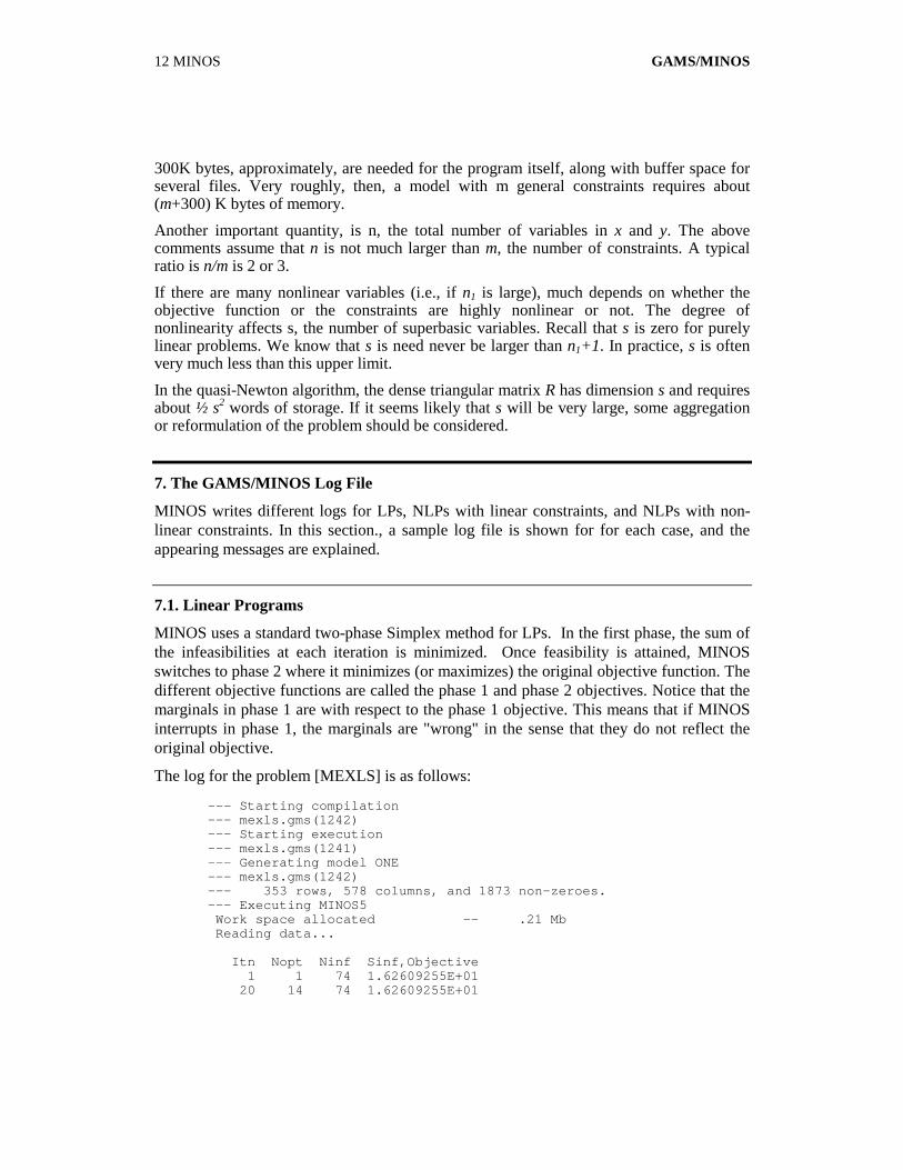
7.1. Linear Programs

MINOS uses a standard two-phase Simplex method for LPs. In the first phase, the sum ofthe infeasibilities at each iteration is minimized. Once feasibility is attained, MINOSswitches to phase 2 where it minimizes (or maximizes) the original objective function. Thedifferent objective functions are called the phase 1 and phase 2 objectives. Notice that themarginals in phase 1 are with respect to the phase 1 objective. This means that if MINOSinterrupts in phase 1, the marginals are "wrong" in the sense that they do not reflect theoriginal objective.

The log for the problem [MEXLS] is as follows:

--- Starting compilation--- mexls.gms(1242)--- Starting execution--- mexls.gms(1241)--- Generating model ONE--- mexls.gms(1242)--- 353 rows, 578 columns, and 1873 non-zeroes.--- Executing MINOS5 Work space allocated -- .21 Mb Reading data...

Itn Nopt Ninf Sinf,Objective 1 1 74 1.62609255E+01 20 14 74 1.62609255E+01

GAMS/MINOS MINOS 13

40 4 67 1.40246211E+01 60 14 55 1.10065392E+01 80 12 42 8.35651175E+00

Itn Nopt Ninf Sinf,Objective 100 6 31 7.21650054E+00 120 21 20 6.65998885E+00 140 13 11 5.77113823E+00 160 1 8 2.35537706E+00 180 4 5 9.58810903E-01

Itn Nopt Ninf Sinf,Objective 200 9 2 3.16184199E-01

Itn 208 -- Feasible solution. Objective = 4.283788540E+04

220 2 0 4.11169434E+04 240 25 0 3.88351313E+04 260 1 0 3.77495457E+04 280 11 0 3.66399964E+04

Itn Nopt Ninf Sinf,Objective 300 2 0 3.30955215E+04 320 2 0 3.09919632E+04 340 5 0 2.84521363E+04 360 1 0 2.76671551E+04 380 2 0 2.76055456E+04 Itn 392 -- 80 nonbasics set on bound, basics recomputed

Itn 392 -- Feasible solution. Objective = 2.756959890E+04

EXIT -- OPTIMAL SOLUTION FOUND

Major, Minor itns 1 392 Objective function 2.7569598897150E+04 Degenerate steps 83 21.17 Norm X, Norm PI 2.10E+01 4.49E+04 Norm X, Norm PI 8.05E+03 1.06E+02 (unscaled)--- Restarting execution--- mexls.gms(1242)--- Reading solution for model ONE--- All done

Considering each section of the log file above in order:

------------------------------------------------------------------ Work space allocated -- .21 Mb Reading data...------------------------------------------------------------------

When MINOS is loaded, the amount of memory needed is first estimated. This estimate isbased on statistics like the number of rows, columns and non-zeros. This amount ofmemory is then allocated and the problem is then loaded into MINOS.

Next, the MINOS iteration log begins. In the beginning, a feasible solution has not yetbeen found, and the screen log during this phase of the search looks like:

14 MINOS GAMS/MINOS

-------------------------------------- --------------------------- Itn Nopt Ninf Sinf,Objective 1 1 74 1.62609255E+01------------------------------------------------------------------

The first column gives the iteration count. A simplex iteration corresponds to a basischange. Nopt means "Number of non-optimalities" which refers to the number ofmarginals that do not have the correct sign (i.e. they do not satisfy the optimalityconditions), and Ninf means "Number of infeasibilities" which refers to the number ofinfeasible constraints . The last column gives the "Sum of infeasibilities" in phase 1 (whenNinf > 0) or the Objective in phase 2.

As soon as MINOS finds a feasible solution, it returns a message similar to the one belowthat appears for the example discussed:

------------------------------------------------------------------ Itn 208 -- Feasible solution. Objective = 4.283788540E+04------------------------------------------------------------------

MINOS found a feasible solution and will switch from phase 1 to phase 2. During phase 2(or the search once feasibility has been reached), MINOS returns a message that lookslike:

------------------------------------------------------------------ Itn 392 -- 80 nonbasics set on bound, basics recomputed------------------------------------------------------------------

Even non-basic variables may not be exactly on their bounds during the optimizationphase. MINOS uses a sliding tolerance scheme to fight stalling as a result of degeneracy.Before it terminates it wants to get the "real" solution. The non-basic variables aretherefore reset to their bounds and the basic variables are recomputed to satisfy theconstraints Ax = b. If the resulting solution is infeasible or non-optimal, MINOS willcontinue iterating. If necessary, this process is repeated one more time. Fortunately,optimality is usually confirmed very soon after the first "reset". In the example discussed,feasibility was maintained after this excercise, and the resulting log looks like:

------------------------------------------------------------------ Itn 392 -- Feasible solution. Objective = 2.756959890E+04------------------------------------------------------------------

MINOS has found the optimal solution, and then exits with the following summary:

------------------------------------------------------------------ Major, Minor itns 1 392 Objective function 2.7569598897150E+04 Degenerate steps 83 21.17 Norm X, Norm PI 2.10E+01 4.49E+04 Norm X, Norm PI 8.05E+03 1.06E+02 (unscaled)------------------------------------------------------------------

GAMS/MINOS MINOS 15

For an LP, the number of major iterations is always one. The number of minor iterations isthe number of Simplex iterations.

Degenerate steps are ones where a Simplex iteration did not do much other than a basischange: two variables changed from basic to non-basic and vice versa, but none of theactivity levels changed. In this example there were 83 degenerate iterations, or 21.17% ofthe total 392 iterations.

The norms ||x|| , ||pi|| are also printed both before and after the model is unscaled. Ideallythe scaled ||x|| should be about 1 (say in the range 0.1 to 100), and ||pi|| should be greaterthan 1. If the scaled ||x|| is closer to 1 than the final ||x|| , then scaling was probablyhelpful. Otherwise, the model might solve more efficiently without scaling.

If ||x|| or ||pi|| are several orders of magnitude different before and after scaling, you maybe able to help MINOS by scaling certain sets of variables or constraints yourself (forexample, by choosing different units for variables whose final values are very large.)

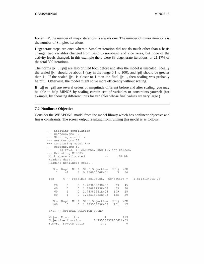
7.2. Nonlinear Objective

Consider the WEAPONS model from the model library which has nonlinear objective andlinear constraints. The screen output resulting from running this model is as follows:

--- Starting compilation--- weapons.gms(59)--- Starting execution--- weapons.gms(57)--- Generating model WAR--- weapons.gms(59)--- 13 rows, 66 columns, and 156 non-zeroes.--- Executing MINOS5 Work space allocated -- .06 Mb Reading data... Reading nonlinear code...

Itn Nopt Ninf Sinf,Objective Nobj NSB 1 -1 3 9.75000000E+01 3 64

Itn 6 -- Feasible solution. Objective = 1.511313490E+03

20 5 0 1.70385909E+03 23 45 40 3 0 1.73088173E+03 63 30 60 1 0 1.73381961E+03 109 25 80 1 0 1.73518225E+03 155 20

Itn Nopt Ninf Sinf,Objective Nobj NSB 100 0 0 1.73555465E+03 201 17

EXIT -- OPTIMAL SOLUTION FOUND

Major, Minor itns 1 119 Objective function 1.7355695798562E+03 FUNOBJ, FUNCON calls 245 0

16 MINOS GAMS/MINOS

Superbasics, Norm RG 18 2.18E-08 Degenerate steps 2 1.68 Norm X, Norm PI 2.74E+02 1.00E+00 Norm X, Norm PI 2.74E+02 1.00E+00 (unscaled)--- Restarting execution--- weapons.gms(59)--- Reading solution for model WAR--- All done

The parts described in the LP example will not be repeated - only the new additions willbe discussed.

------------------------------------------------------------------ Reading nonlinear code...------------------------------------------------------------------

Besides reading the matrix GAMS/MINOS also reads the instructions that allow theinterpreter to calculate nonlinear function values and their derivatives.

The iteration log looks slightly different from the earlier case, and has a couple ofadditional columns.

------------------------------------------------------------------ Itn Nopt Ninf Sinf,Objective Nobj NSB 1 -1 3 9.75000000E+01 3 64------------------------------------------------------------------

The column Nobj gives the number of times MINOS calculated the objective and itsgradient. The column NSB contains the number of superbasics. In MINOS, variables aretyped basic, non-basic or superbasic. The number of superbasics once the number settlesdown (there may be rather more at the beginning of a run) is a measure of the nonlinearityof the problem. The final number of superbasics will never exceed the number ofnonlinear variables, and in practice will often be much less (in most cases less than a fewhundred).

There is not much that a modeler can do in this regard, but it is worth remembering thatMINOS works with a dense triangular matrix R (which is used to approximate the reducedHessian) of that dimension. Optimization time and memory requirements will besignificant if there are more than two or three hundred superbasics.

Once the optimum solution has been found, MINOS exits after printing a search summarythat is slightly different from the earlier case.

------------------------------------------------------------------ Major, Minor itns 1 119------------------------------------------------------------------

As in the earlier case, there is always only one major iteration. Each iteration of thereduced-gradient method is called a minor iteration.

------------------------------------------------------------------ FUNOBJ, FUNCON calls 245 0------------------------------------------------------------------

GAMS/MINOS MINOS 17

FUNOBJ is the number of times MINOS asked the interpreter to evaluate the objectivefunction and its gradients. FUNCON means the same for the nonlinear constraints. As thismodel has only linear constraints, the number is zero.

If you know that your model has linear constraints but FUNCON turns out to be positive,your nonlinear objective function is being regarded as a nonlinear constraint. You canimprove MINOS’s efficiency by following some easy rules. Please see "Objective: specialtreatment of in NLP" in the index for the GAMS User’s Guide.

------------------------------------------------------------------ Superbasics, Norm RG 18 2.18E-08------------------------------------------------------------------

The number of superbasic variables in the final solution is reported and also the norm ofthe reduced gradient (which should be close to zero for an optimal solution).

7.3. Nonlinear constraints

For models with nonlinear constraints the log is more complicated. CAMCGE from themodel library is such an example, and the screen output resulting from running it is shownbelow:

--- Starting compilation--- camcge.gms(444)--- Starting execution--- camcge.gms(435)--- Generating model CAMCGE--- camcge.gms(444)--- 243 rows, 280 columns, and 1356 non-zeroes.--- Executing MINOS5 Work space allocated -- .36 Mb Reading data... Reading nonlinear code...

Major Minor Ninf Sinf,Objective Viol RG NSB Ncon Penalty Step 1 0 1 0.000000E+00 1.3E+02 0.0E+00 184 3 6.8E-01 1.0E+00 2 40T 30 0.00000000E+00 8.8E+01 7.3E+02 145 4 6.8E-01 1.0E+00 3 40T 30 0.00000000E+00 8.8E+01 1.7E+01 106 5 6.8E-01 1.0E+00 4 40T 30 0.00000000E+00 8.8E+01 2.1E+01 66 6 6.8E-01 1.0E+00 5 40T 25 0.00000000E+00 8.8E+01 1.7E+01 26 7 6.8E-01 1.0E+00 6 29 0 1.91734197E+02 2.6E-03 0.0E+00 0 9 6.8E-01 1.0E+00 7 0 0 1.91734624E+02 2.3E-08 0.0E+00 0 10 1.4E+00 1.0E+00 8 0 0 1.91734624E+02 4.5E-13 0.0E+00 0 11 1.4E+00 1.0E+00 9 0 0 1.91734624E+02 6.8E-13 0.0E+00 0 12 0.0E+00 1.0E+00

EXIT -- OPTIMAL SOLUTION FOUND

Major, Minor itns 9 189 Objective function 1.9173462423688E+02 FUNOBJ, FUNCON calls 8 12 Superbasics, Norm RG 0 0.00E+00 Degenerate steps 0 .00

18 MINOS GAMS/MINOS

Norm X, Norm PI 1.37E+03 2.88E+01 Norm X, Norm PI 8.89E+02 7.01E+01 (unscaled) Constraint violation 6.82E-13 7.66E-16--- Restarting execution--- camcge.gms(444)--- Reading solution for model CAMCGE--- All done

Note that the iteration log is different from the two cases discussed above. A smallsection of this log is shown below.

--------------------------------------------------------------------Major Minor Ninf Sinf,Objective Viol RG NSB Ncon Penalty Step1 0 1 0.00000000E+00 1.3E+02 0.0E+00 184 3 6.8E-01 1.0E+002 40T 30 0.00000000E+00 8.8E+01 7.3E+02 145 4 6.8E-01 1.0E+00--------------------------------------------------------------------

Two sets of iterations - Major and Minor, are now reported. A description of the variouscolumns present in this log file follows:

Major A major iteration involves linearizing the nonlinear constraints andperforming a number of minor iterations on the resulting subproblem.The objective for the subproblem is an augmented Lagrangian, not thetrue objective function.

Minor The number of minor iterations performed on the linearized subproblem.If it is a simple number like 29, then the subproblem was solved tooptimality. Here, 40T means that the subproblem was terminated. (Thereis a limit on the number of minor iterations per major iteration, and bydefault this is 40.) in general the T is not something to worry about.Other possible flags are I and U, which mean that the subproblem wasInfeasible or Unbounded. MINOS may have difficulty if these keepoccurring.

Ninf The number of infeasibilities at the end of solving the subproblem. It is0 if the linearized constraints were satisfied. It then means that all linearconstraints in the original problem were satisfied, but only Viol (below)tells us about the nonlinear constraints.

Objective The objective function for the original nonlinear program.

Viol The maximum violation of the nonlinear constraints.

RG The reduced gradient for the linearized subproblem. If Viol and RG aresmall and the subproblem was not terminated, the original problem hasalmost been solved.

NSB The number of superbasics. If ninf > 0 at the beginning, it will notmatter too much if NSB is fairly large. It is only when ninf reaches 0 thatMINOS starts working with a dense matrix R of dimension NSB.

GAMS/MINOS MINOS 19

Ncon The number of times MINOS has evaluated the nonlinear constraints andtheir derivatives.

Penalty The current value of the penalty parameter in the augmented Lagrangian(the objective for the subproblems). If the major iterations appear to beconverging, MINOS will decrease the penalty parameter. If there appearsto be difficulty, such as unbounded subproblems, the penalty parameterwill be increased.

Step The step size taken towards the solution suggested by the last majoriteration. Ideally this should be 1.0, especially near an optimum. Thequantity Viol should then decrease rapidly. If the subproblem solutionsare widely different, MINOS may reduce the step size under control ofthe Major Damping parameter.

The final exit summary has an additional line in this case. For the problem beingdescribed, this line looks like:

------------------------------------------------------------------ Constraint violation 6.82E-13 7.66E-16------------------------------------------------------------------

The first number is the largest violation of any of the nonlinear constraints (the final valueof Viol). The second number is the relative violation, Viol/(1.0 + ||x||) . It may be moremeaningful if the solution vector x is very large.

For an optimal solution, these numbers must be small.

Note: The CAMCGE model (like many CGE models or other almost square systems) canbetter be solved with the MINOS option Start Assigned Nonlinears Basic. It can be noticedin the log that the algorithm starts out with lots of super basics (corresponding to the non-linear variables). MINOS starts with removing these superbasics, and only then startsworking towards an optimal solution.

8. Detailed Description of MINOS Options

The following is an alphabetical list of the keywords that may appear in theGAMS/MINOS options file, and a description of their effect. The letters I and r denoteinteger and real values. The number ε denotes machine precision (typically 10-15 or 10-16).Options not specified will take the default values shown.

Check frequency i Every i-th iteration after the most recent basis factorization,a numerical test is made to see if the current solution xsatisfies the general linear constraints (including linearizednonlinear constraints, if any). The constraints are of the formAx + s = 0 where s is the set of slack variables. To performthe numerical test, the residual vector r = Ax + s is

20 MINOS GAMS/MINOS

computed. If the largest component of r is judged to be toolarge, the current basis is refactorized and the basic variablesare recomputed to satisfy the general constraints moreaccurately.

(Default = 30)

Completion Full/Partial When there are nonlinear constraints, this determineswhether subproblems should be solved to moderate accuracy(partial completion), or to full accuracy (full completion),GAMS/MINOS implements the option by using two sets ofconvergence tolerances for the subproblems.

Use of partial completion may reduce the work during earlymajor iterations, unless the Minor iterations limit is active.The optimal set of basic and superbasic variables willprobably be determined for any given subproblem, but thereduced gradient may be larger than it would have been withfull completion.

An automatic switch to full completion occurs when itappears that the sequence of major iterations is converging.The switch is made when the nonlinear constraint error isreduced below 100*(Row tolerance), the relative change inλk is 0.1 or less, and the previous subproblem was solved tooptimality.

Full completion tends to give better Langrange-multiplierestimates. It may lead to fewer major iterations, but mayresult in more minor iterations.

(Default = FULL)

Crash option i If a restart is not being performed, an initial basis will beselected from certain columns of the constraint matrix (AI).The value of i determines which columns of A are eligible.Columns of I are used to fill “gaps” where necessary.

If i > 0, three passes are made through the relevant columnsof A, searching for a basis matrix that is essentiallytriangular. A column is assigned to “pivot” on a particularrow if the column contains a suitably large element in a rowthat has not yet been assigned.(The pivot elements ultimatelyform the diagonals of the triangular basis).

Pass 1 selects pivots from free columns (corresponding tovariables with no upper and lower bounds). Pass 2 requirespivots to be in rows associated with equality (=E=)constraints. Pass 3 allows the pivots to be in inequality rows.

For remaining (unassigned) rows, the associated slackvariables are inserted to complete the basis.

GAMS/MINOS MINOS 21

(Default = 1)

0 The initial basis will contain only slack variables: B = I

1 All columns of A are considered (except those excluded bythe Start assigned nonlinears option).

2 Only the columns of A corresponding to the linear variablesy will be considered.

3 Variables that appear nonlinearly in the objective will beexcluded from the initial basis.

4 Variables that appear nonlinearly in the constraints will beexcluded from the initial basis.

Crash tolerance r The Crash tolerance r allows the starting procedure CRASHto ignore certain “small” nonzeros in each column of A. Ifamax is the largest element in column j, other nonzeros aij inthe column are ignored if |aij| < amax.r. To be meaningful, rshould be in the range 0 ≤ r < 1).

When r > 0.0 the basis obtained by CRASH may not bestrictly triangular, but it is likely to be nonsingular andalmost triangular. The intention is to obtain a starting basiscontaining more columns of A and fewer (arbitrary) slacks.A feasible solution may be reached sooner on someproblems.

For example, suppose the first m columns of A are thematrix shown under LU factor tolerance ; i.e., a tridiagonalmatrix entries -1, 4, -1. To help CRASH choose all mcolumns for the initial basis, we could specify Crashtolerance r for some value of r > 0.25.

(Default = 0.1)

Damping parameter r See Major Damping Parameter

(Default = 2.0)

Debug level i This causes various amounts of information to be output.Most debug levels will not be helpful to GAMS users, butthey are listed here for completeness.

(Default = 0)

0 No debug output.

2 (or more) Output from M5SETX showing the maximum residual after arow check.

40 Output from LU8RPC (which updates the LU factors of the

22 MINOS GAMS/MINOS

basis matrix), showing the position of the last nonzero in thetransformed incoming column

50 Output from LU1MAR (which updates the LU factors eachrefactorization), showing each pivot row and column and thedimensions of the dense matrix involved in the associatedelimination.

100 Out from M2BFAC and M5LOG listing the basic andsuperbasic variables and their values at every iteration.

Expand frequency i This option is part of anti-cycling procedure designed toguarantee progress even on highly degenerate problems.

For linear models, the strategy is to force a positive step atevery iteration, at the expense of violating the bounds on thevariables by a small amount. Suppose the specifiedfeasibility tolerance is δ.

Over a period of i iterations, the tolerance actually used byGAMS/MINOS increases from 0.5 δ to δ (in steps 0.58 δ / i).

For nonlinear models, the same procedure is used foriterations in which there is only one superbasic variable.(Cycling can occur only when the current solution is at avertex of the feasible region.) Thus, zero steps are allowed ifthere is more than one superbasic variable, but otherwisepositive steps are enforced.

Increasing i helps reduce the number of slightly infeasiblenonbasic basic variables (most of which are eliminatedduring a resetting procedure). However, it also diminishesthe freedom to choose a large pivot element (see Pivottolerance).

(Default = 10000)

Factorization frequency i At most i basis changes will occur between factori-zations ofthe basis matrix.

With linear programs, the basis factors are usually updatedevery iteration. The default i is reasonable for typicalproblems. Higher values up to i =100 (say) may be moreefficient on problems that are extremely sparse and wellscaled.

When the objective function is nonlinear, fewer basisupdates will occur as an optimum is approached. Thenumber of iterations between basis factorizations willtherefore increase. During these iterations a test is made

GAMS/MINOS MINOS 23

regularly (according to the Check frequency) to ensure thatthe general constraints are satisfied. If necessary the basiswill be re-factorized before the limit of i updates is reached.

When the constraints are nonlinear, the Minor iterationslimit will probably preempt i .

(Default = 50)

Feasibility tolerance r When the constraints are linear, a feasible solution is one inwhich all variables, including slacks, satisfy their upper andlower bounds to within the absolute tolerance r. (Sinceslacks are included, this means that the general linearconstraints are also satisfied to within r.)

GAMS/MINOS attempts to find a feasible solution beforeoptimizing the objective function. If the sum ofinfeasibilities cannot be reduced to zero, the problem isdeclared infeasible. Let SINF be the corresponding sum ofinfeasibilities, If SINF is quite small, it may be appropriateto raise r by a factor of 10 or 100. Otherwise, some error inthe data should be suspected.

If SINF is not small, there may be other points that have asignificantly smaller sum of infeasibilities. GAMS/MINOSdoes not attempt to find a solution that minimizes the sum.

If Scale option = 1 or 2, feasibility is defined in terms of thescaled problem (since it is then more likely to bemeaningful)

A nonlinear objective function F(x) will be evaluated only atfeasible points. If there are regions where F(x) is undefined,every attempt should be made to eliminate these regionsfrom the problem. For example, for a function F(x) =sqrt(x1) + log(x2), it should be essential to place lowerbounds on both variables. If Feasibility tolerance = 10-6, thebounds x1 > 10-5 and x2 > 10-4 might be appropriate. (The logsingularity is more serious; in general, keep variables as faraway from singularities as possible.)

If the constraints are nonlinear, the above comments apply toeach major iteration. A “feasible solution” satisfies thecurrent linearization of the constraints to within thetolerance r. The associated subproblem is said to be feasible.

As for the objective function, bounds should be used to keepx more than r away from singularities in theconstraint functions f(x).

At the start of major iteration k, the constraint functions f(xk)

24 MINOS GAMS/MINOS

are evaluated at a certain point xk. This point always satisfiesthe relevant bounds (l < xk < u), but may not satisfy thegeneral linear constraints.

During the associated minor iterations, F(x) and f(x) will beevaluated only at points x that satisfy the bound and thegeneral linear constraints (as well as the linearized nonlinearconstraints).

If a subproblem is infeasible, the bounds on the linearizedconstraints are relaxed temporarily, in several stages.

Feasibility with respect to the nonlinear constraintsthemselves is measured against the Row tolerance (notagainst r. The relevant test is made at the start of a majoriteration.

(Default = 1.0E-6)

Hessian dimension r This specifies than an r X r triangular matrix R is to beavailable for use by the quasi-Newton algorithm (toapproximate the reduced Hessian matrix according to ZTHZ≈ RTR. Suppose there are s superbasic variables at aparticular iteration. Whenever possible, r should be greaterthan s.

If r > s, the first s columns of R will be used to approximatethe reduced Hessian in the normal manner. If there are nofurther changes to the set of superbasic variables, the rate ofconvergence will ultimately be superlinear.

If r < s, a matrix of the form,

RR

Dr=

0

will be used to approximate the reduced Hessian, Where Rr

is an r X r upper triangular matrix and D is a diagonalmatrix of order s - r. The rate of convergence will no longerbe superlinear (and may be arbitrarily slow.

The storage required if of the order ½ r2, which is substantialif r is as large as 200 (say). In general, r should be slightover-estimate of the final number of superbasic variables,whenever storage permits. It need not be larger than n1+1,where n1 is the number of nonlinear variables. For manyproblems it can be much smaller than n1.

If Superbasics limit s is specified, the default value of r isthe same number, s (and conversely). This is a safeguard to

GAMS/MINOS MINOS 25

ensure super-linear convergence wherever possible. Ifneither r nor s is specified, GAMS chooses values for both,using certain characteristics of the problem.

(Default = Superbasics limit)

Iterations limit i This is maximum number of minor iterations allowed (i.e.,iterations of the simplex method or the reduced-gradientmethod). This option, if set, overrides the GAMS ITERLIMspecification. If i = 0, no minor iterations are performed, butthe starting point is tested for both feasibility and optimality.

Iters or Itns are alternative keywords.

(Default = 1000)

Lagrangian Yes/No This determines the form of the objective function used forthe linearized subproblems. The default value yes is highlyrecommended. The Penalty parameter value is then alsorelevant.

If No is specified, the nonlinear constraint functions will beevaluated only twice per major iteration. Hence this optionmay be useful if the nonlinear constraints are very expensiveto evaluate. However, in general there is a great risk thatconvergence may not occur.

(Default = yes)

Linesearch tolerance r For nonlinear problems, this controls the accuracy withwhich a step-length α is located in the one-dimensionalproblem

Minimize α F(x + αp)subject to 0 < α ≤ β

A linesearch occurs on most minor iterations for which x isfeasible. [If the constraints are nonlinear, the function beingminimized is the augmented Lagrangian in equation (5).]

r must be a real value in the range 0.0 < r < 1.0.

The default value r = 0.1 requests a moderately accuratesearch. It should be satisfactory in most cases.

If the nonlinear functions are cheap to evaluate, a moreaccurate search may be appropriate: try r = 0.01 or r =0.001. The number of iterations should decrease, and thiswill reduce total run time if there are many linear ornonlinear constraints.

26 MINOS GAMS/MINOS

If the nonlinear function are expensive to evaluate, a lessaccurate search may be appropriate; try r = 0.5 or perhaps r= 0.9. (The number of iterations will probably increase butthe total number of function evaluations may decreaseenough to compensate.)

(Default = 0.1)

Log Frequency i In general, one line of the iteration log is printed every i-thminor iteration. A heading labels the printed items, whichinclude the current iteration number, the number and sum offeasibilities (if any), the subproblem objective value (iffeasible), and the number of evaluations of the nonlinearfunctions,

A value such as i = 10, 100 or larger is suggested for thoseinterested only in the final solution

Log frequency 0 may be used as shorthand for Log frequency99999.

If Print level > 0, the default value of i is 1. If Print level =0, the default value of i is 100. If Print level = 0 and theconstraints are nonlinear, the minor iteration log is notprinted (and the Log frequency is ignored). Instead, one lineis printed at the beginning of each major iteration.

(Default = 1 or 100)

LU factor tolerance r1 LU update tolerance r2

LU Singularity tolerance r3

The first two tolerances affect the stability and sparsity ofthe basis factorization B = LU during re-factorization andupdates respectively. The values specified must satisfy ri ≥1.0. The matrix L is a product of matrices of the form.

11µ

where the multipliers µ will satisfy |µ| < ri.

1. The default values ri = 10.0 usually strike a goodcompromise between stability and sparsity.2. For large and relatively dense problems, ri = 25.0 (say)may give a useful improvement it sparsity without impairingstability to a serious degree.3. For certain very regular structures (e.g., band matrices) itmay be necessary to set and r1 and/or r2 to values smallerthan the default in order to achieve stability. For example, if

GAMS/MINOS MINOS 27

the columns of A include a sub-matrix of the form

4 11 4 1

1 4

−− −

−

it would be judicious to set both r1 and r2 to values in therange 1.0 < ri < 4.0. The singularity tolerance r3 helps guardagainst ill-conditioned basis matrices. When the basis isrefactorized, the diagonal elements of U are tested asfollows: if |Ujj| ≤ r3 or |Ujj| < r3 maxi |Ujj| , the j-th columnof the basis is replaced by the corresponding slack variable.(This is most likely to occur after a restart, or at the start of amajor iteration.)

In some cases , the Jacobian matrix may converge to valuesthat make the basis could become very ill-conditioned andthe optimization could progress very slowly (if at all).Setting r3 = 1.0E-5, say, may help cause a judicious changeof basis.

(Default values: r1 = 10.0, r2 = 10.0, r3 = ε2/3 ≈ 10-11)

Major damping parameter r The parameter may assist convergence on problems thathave highly nonlinear constraints. It is intended to preventlarge relative changes between subproblem solutions (xk, λk)and (xk+1, λk+1). For example, the default value 2.0 preventsthe relative change in either xk or λk from exceeding 200percent. It will not be active on well behaved problems.

The parameter is used to interpolate between the solutions atthe beginning and end of each major iteration. Thus xk+1 andλk+1 are changed to

xk + σ (xk+1 - xk) and λk + σ (λk+1 - λk)

for some step-length σ < 1. In the case of nonlinear equation(where the number of constraints is the same as the numberof variables) this gives a damped Newton method.

This is very crude control. If the sequence of majoriterations does not appear to be converging, one should firstre-run the problem with a higher Penalty parameter (say 10or 100 times the default ρ). (Skip this re-run in the case ofnonlinear equations: there are no degrees of freedom and thevalue of ρ is irrelevant.)

If the subproblem solutions continue to change violently, tryreducing r to 0.2 or 0.1 (say).

28 MINOS GAMS/MINOS

For implementation reason, the shortened step to σ appliesto the nonlinear variables x, but not to the linear variables yor the slack variables s. This may reduce the efficiency ofthe control.

(Default = 2.0)

Major iterations i This is maximum number of major iterations allowed. It isintended to guard against an excessive number oflinearizations of the nonlinear constraints, since in somecases the sequence of major iterations my not converge. Theprogress of the major iterations can be best monitored usingPrint level 0 (the default).

(Default = 50)

Minor damping parameter r This parameter limits the change in x during a linesearch. Itapplies to all nonlinear problems, once a “feasible solution”or “feasible subproblem” has been found.

A linesearch of the form minimizeα F(x + αp) isperformed over the range 0 < α ≤ β, where β is the step tothe nearest upper or lower bound on x. Normally, the firststep length tried is α1 = min (1,β).

In some cases, such as F(x) = aebx or F(x) = axb, even amoderate change in the components of r can lean to floating-point overflow. The parameter r is therefore used to define alimit

β’ = r (1 + ||x||)/||p||

and the first evaluation of F(x) is at the potentially smallersteplength α1 = min(1, β, β’).

Wherever possible, upper and lower bounds on x should beused to prevent evaluation of nonlinear functions atmeaningless points. The Minor damping parameter providesan additional safeguard. The default value r = 2.0 shout notaffect progress on well behaved problems, but setting r = 0.1or 0.01 may be helpful when rapidly varying function arepresent. A “good” starting point may be required. Animportant application is to the class of nonlinear leastsquares problems.

In case where several local optima exist, specifying a smallvalue for r may help locate an optima near the starting point.

(Default = 2.0)

GAMS/MINOS MINOS 29

Minor iterations i This is the maximum number of minor iterations allowedbetween successive linearizations of the nonlinearconstraints.

A moderate value (e.g., 20 ≤ i ≤ 50 ) prevents excessiveefforts being expended on early major iterations, but allowslater subproblems to be solved to completion.

The limit applies to both infeasible and feasible iterations. Insome cases, a large number of iterations, (say K) might berequired to obtain a feasible subproblem. If good startingvalues are supplied for variables appearing nonlinearly in theconstraints, it may be sensible to specify > K, to allow thefirst major iteration to terminate at a feasible (and perhapsoptimal) subproblem solution. (If a “good” initialsubproblem is arbitrarily interrupted by a small I thsubsequent linearization may be less favorable than thefirst.)

In general it is unsafe to specify value as small as i = 1or 2.)even when an optimal solution has been reached, a fewminor iterations may be needed for the correspondingsubproblem to be recognized as optimal.)

The Iteration limit provides an independent limit on the totalminor iterations (across all subproblems).

If the constraints are linear, only the Iteration limit applies:the minor iterations value is ignored.

(Default = 40)

Multiple price i “pricing” refers to a scan of the current non-basic variablesto determine if any should be changed from their value (byallowing them to become superbasic or basic).

If multiple pricing in effect, the i best non-basic variables areselected for admission of appropriate sign.) If partial pricingis also in effect , the best i best variables are selected fromthe current partition of A and I.

The default i = 1 is best for linear programs, since anoptimal solution will have zero superbasic variables.

Warning : If i > 1, GAMS/MINOS will use the reduced-gradient method (rather than the simplex method ) even onpurely linear problems. The subsequent iterations of notcorrespond to the efficient “minor iterations” carried out becommercial linear programming system using multiplepricing. (In the latter systems, the classical simplex methodis applied to a tableau involving i dense columns ofdimension m, and i is therefore limited for storage reasons

30 MINOS GAMS/MINOS

typically to the range 2 ≤ i ≤ 7.)

GAMS/MINOS varies all superbasic variablessimultaneously. For linear problems its storage requirementsare essentially independent of i . Larger values of i aretherefore practical, but in general the iterations and timerequired when i > 1 are greater than when the simplexmethod is used (i=1) .

On large nonlinear problems it may be important to set i >1if the starting point does not contain many superbasicvariables. For example, if a problem has 3000 variables and500 of them are nonlinear, the optimal solution may wellhave 200 variables superbasic. If the problem is solved inseveral runs, it may be beneficial to use i = 10 (say) forearly runs, until it seems that the number of superbasics hasleveled off.

If Multiple price i is specified , it is also necessary to specifySuperbasic limit s for some s > i.

(Default = 1)

Optimality tolerance r This is used to judge the size of the reduced gradients dj = gj

- πTaj, where gj is the gradient of the objective functioncorresponding to the j-th variable. aj is the associatedcolumn of the constraint matrix (or Jacobian), and π is theset of dual variables.

By construction, the reduced gradients for basic variablesare always zero. Optimality will be declared if the reducedgradients for nonbasic variables at their lower or upperbounds satisfy

dj / ||π|| ≥ - r or dj / ||π|| ≤ r

respectively, and if dj / ||π|| ≤ r for superbasic variables.

In the ||π|| is a measure of the size of the dual variables. It isincluded to make the tests independents of a scale factor onthe objective function.

The quantity actually used is defined by

=∑i 1

, || || max{ / , }π σ= m 1

so that only large scale factors are allowed for.

If the objective is scaled down to be small, the optimalitytest effectively reduced to comparing Dj against r.

GAMS/MINOS MINOS 31

(Default = 1.0E-6)

Partial Price i This parameter is recommended for large problems that havesignificantly more variables than constraints. It reduces thework required for each “pricing” operation (when a nonbasicvariable is selected to become basic or superbasic).

When i = 1, all columns of the constraints matrix (A I) aresearched.

Otherwise, Aj and I are partitioned to give i roughly equalsegments Aj , Ij (j = 1 to i). If the previous search wassuccessful on Aj-1 , Ij -1, the next search begins on thesegments Aj , Ij. (All subscripts here are modulo i.)

If a reduced gradient is found that is large than somedynamic tolerance, the variable with the largest such reducedgradient (of appropriate sign) is selected to becomesuperbasic. (several may be selected if multiple pricing hasbeen specified.) IF nothing is found, the search continues onthe next segments Aj + 1, Ij + 1 and so on.

Partial price t (or t/2 or t/3) may be appropriate for time-stage models having t time periods.

(Default = 10 for LPs, or 1 for NLPs)Penalty Parameter r This specifies the value of ρ in the modified augmented

Lagrangian. It is used only when Lagrangian = yes (thedefault setting).

For early runs on a problem is known to be unknowncharacteristics, the default value should be acceptable. If theproblem is problem is known to be highly nonlinear, specifya large value, such as 10 times the default. In general, apositive value of ρ may be necessary of known to ensureconvergence, even convex programs.

On the other hand, if ρ is too large, the rate of convergencemay be unnecessarily slow. If the functions are not highlynonlinear or a good starting point is known, it will often besafe to specify penalty parameter 0.0

Initially, use a moderate value for r (such as the default) anda reasonably low Iterations and/or major iterations limit.

If successive major iterations appear to be terminating withradically different solutions, the penalty parameter should beincreased. (See also the Major damping parameter. )

If there appears to be little progress between major iteration,it may help to reduce the penalty parameter.

(Default = 100.0/m1)

32 MINOS GAMS/MINOS

Pivot Tolerance r Broadly speaking, the pivot tolerance is used to preventcolumns entering the basis if they would cause the basis tobecome almost singular. The default value of r should besatisfactory in most circumstances.

When x changes to x + αp for some search direction p, a“ratio test” is used to determine which component of xreaches an upper or lower bound first. The correspondingelement of p is called the pivot element.

For linear problems, elements of P are ignored (andtherefore cannot be pivot elements) if they are smaller thanthe pivot tolerance r.

For nonlinear problems, elements smaller than r ||p|| areignored.

It is common (on “degenerate” problems) for two or morevariables to reach a bound at essentially the same time. Insuch cases, the Feasibility tolerance (say t) provides somefreedom to maximize the pivot element and thereby improvenumerical stability. Excessively small values of t should notbe specified.

To a lesser extent, the Expand frequency (say f) alsoprovides some freedom to maximize pivot the element.Excessively large values of f should therefore not bespecified .

(Default = ε2/3 ≈ 10-11)

Print level i This varies the amount of information that will be outputduring optimization.

Print level 0 sets the default Log and summary frequenciesto 100. It is then easy to monitor the progress of run.

Print level 1 (or more) sets the default Log and summaryfrequencies to 1, giving a line of output for every minoriteration. Print level 1 also produces basis statistics., i.e.,information relating to LU factors of the basis matrixwhenever the basis is re-factorized.

For problems with nonlinear constraints, certain quantitiesare printed at the start of each major iteration. The value ofi is best thought of as a binary number of the form

Print level JFLXB

where each letter stand for a digit that is either 0 or 1. Thequantities referred to are:

GAMS/MINOS MINOS 33

B Basis statistics, as mentioned above.

X xk, the nonlinear variables involved in the objective functionor the constraints.

L λk, the Lagrange-multiplier estimates for the nonlinearconstraints. (Suppressed if Lagrangian=No, since thenλk=0.)

F f(xk), the values of the nonlinear constraint functions.

J J(xk), the Jacobian matrix.

To obtain output of any item, set the corresponding digit to1, otherwise to 0. For example, Print level 10 sets X=1 andthe other digits equal to zero; the nonlinear variables will beprinted each major iteration.

If J =1, the Jacobian matrix will be output column-wise atthe start of each major iteration. Column j will be precededby the value of the corresponding variable xj and a key toindicate whether the variable is basic, superbasic ornonbasic. (Hence if J = 1, there is no reason to specify X =1 unless the objective contains more nonlinear variables thanthe Jacobian.) A typical line of output is

3 1.250000D+01 BS 1 1.00000D+004 2.00000D+00

which would mean that x3 is basic at value 12.5, and thethird column of the Jacobian has elements of 1.0 and 2.0 inrows 1 and 4. (Note: the GAMS/MINOS row numbers areusually different from the GAMS row numbers; see theSolution option.)

(Default = 0)

Radius of convergence r This determines when the penalty parameter ρ will bereduced (if initialized to a positive value). Both the nonlinearconstraint violation (see ROWERR below) and the relativechange in consecutive Lagrange multiplier estimate must beless than r at the start of a major iteration before ρ is reducedor set to zero.

A few major iterations later, full completion will berequested if not already set, and the remaining sequence ofmajor iterations should converge quadratically to anoptimum.

(Default = 0.01)

34 MINOS GAMS/MINOS

Row Tolerance r This specifies how accurately the nonlinear constraintsshould be satisfied at a solution. The default value is usuallysmall enough, since model data is often specified to aboutthat an accuracy.

Let ROWERR be the maximum component of the residualvector f(x) + A1y - b1, normalized by the size of the solution.Thus

ROWERR = || f(x) + A1y - b1||∞ / (1+XNORM)

Where XNORM is a measure of the size of the currentsolution (x,y). The solution is regarded acceptably feasible ifROWERR ≤ r.

If the problem functions involve data that is known to be oflow accuracy, a larger Row tolerance may appropriate.

(Default = 1.0E-6)

Scale option i Scaling done on the model.

(Default = 2 for LPs, 1 for NLPs)

0 No scaling. If storage is at a premium, this option should beused

1 Linear constraints and variables are scaled by an iterativeprocedure that attempts to make the matrix coefficients asclose as possible to 1.0 (see Fourer, 1982). This willsometimes improve the performance of the solutionprocedures. Scale linear variables is an equivalent option.

2 All constraints and variables are scaled by the iterativeprocedure. Also, a certain additional scaling is performedthat may be helpful if the right-hand side b or the solution xis large. This takes into account columns of (AI) that arefixed or have positive lower bounds or negative upperbounds. Scale nonlinear variables or Scale all variables areequivalent options.

Scale Yes sets the default. (Caution: If all variables arenonlinear, Scale Yes unexpectedly does nothing, becausethere are no linear variables to scale). Scale No suppressesscaling (equivalent to Scale Option 0).

If nonlinear constraints are present, Scale option 1 or 0should generally be rid at first. Scale option 2 gives scalesthat depend on the initial Jacobian, and should therefore beused only if (a) good starting point is provided, and (b) theproblem is not highly nonlinear.

GAMS/MINOS MINOS 35

Scale, print This causes the row-scales r(i) and column-scales c(j) to beprinted. The scaled matrix coefficients are a’ ij = aij c(j)/r(i),and the scaled bounds on the variables, and slacks are l’ j =lj/c(j), u’ j = uj/c(j), where c(j) = r(j-n) if j > n.

If a Scale option has not already been specified, Scale, printsets the default scaling.

Scale Tolerance r All forms except Scale option may specify a tolerance rwhere 0 < r <1 (for example: Scale, Print, Tolerance =0.99). This affects how many passes might be neededthrough the constraint matrix. On each pass, the scalingprocedure computes the ration of the largest and smallestnonzero coefficients in each column:

ρj = maxi |aij| / mini |aij| (aij ≠ 0)

If maxj ρj is less than r times its previous value, anotherscaling pass is performed to adjust the row and columnscales. Raising r from 0.9 to 0.99 (say) usually increases thenumber of scaling passes through A. At most 10 passes aremade.

If a Scale option has not already been specified, Scaletolerance sets the default scaling.

(Default = 0.9)

Solution No/Yes This controls whether or not GAMS/MINOS prints the finalsolution obtained. There is one line of output for eachconstraint and variable. The lines are in the same order as inthe GAMS solution, but the constraints and variables labeledwith internal GAMS/MINOS numbers rather than GAMSnames. (The numbers at the left of each line areGAMS/MINOS “column numbers,” and those at the right ofeach line in the rows section are GAMS/MINOS “slacks”.)

The GAMS/MINOS solution may be useful occasionally tointerpret certain messages that occur during theoptimization, and to determine the final status of certainvariables (basic, superbasic or nonbasic).

(Default = No)

Start assigned nonlinears This option affects the starting strategy when there is nobasis (i.e., for the first solve or when option bratio = 1 isused to reject an existing basis.)

This option applies to all nonlinear variables that have beenassigned non-default initial values and are strictly betweentheir bounds. Free variables at their default value of zero are

36 MINOS GAMS/MINOS

excluded. Let K denote the number of such “assignednonlinear variables.”

Note that the first and fourth keywords are significant.

(Default = superbasic)

Superbasic Specify superbasic for highly nonlinear models, as long as Kis not too large (say K < 100) and the initial values are“good”.

Basic Specify basic for models that are essentially “square” (i.e., ifthere are about as many general constraints as variables).

Nonbasic Specify nonbasic if K is large.

Eligible for crash Specify eligible for Crash for linear or nearly linear models.The nonlinear variables will be treated in the mannerdescribed under Crash option.

Subspace tolerance r This controls the extent to which optimization is confined tothe current set of basic and superbasic variables (Phase 4iterations), before one or more nonbasic variables are addedto the superbasic set (Phase 3).

r must be a real number in the range 0 < r ≤ 1.

When a nonbasic variables xj is made superbasic, theresulting norm of the reduced-gradient vector (for allsuperbasics) is recorded. Let this be ||ZTg0||. (In fact, thenorm will be |dj| , the size of the reduced gradient for thenew superbasic variable xj .

Subsequent Phase 4 iterations will continue at least until thenorm of the reduced-gradient vector satisfies ||ZTg0|| ≤ r||ZTg0|| is the size of the largest reduced-gradient componentamong the superbasic variables.)

A smaller value of r is likely to increase the total number ofiterations, but may reduce the number of basic changes. Alarger value such as r = 0.9 may sometimes lead to improvedoverall efficiency, if the number of superbasic variables hasto increase substantially between the starting point and anoptimal solution.

Other convergence tests on the change in the function beingminimized and the change in the variables may prolongPhase 4 iterations. This helps to make the overallperformance insensitive to larger values of r.

(Default = 0.5)

Summary frequency i A brief form of the iteration log is output to the summary

GAMS/MINOS MINOS 37

file. In general, one line is output every i-th minor iteration.,In an interactive environment, the output normally appears atthe terminal and allows a run to be monitored. If somethinglooks wrong, the run can be manually terminated.

The Summary frequency controls summary output in thesame as the log frequency controls output to the print file

A value such as i = 10 or 100 is often adequate to determineif the SOLVE is making progress. If Print level = 0, thedefault value of i is 100. If Print level > 0, the default valueof i is 1. If Print level = 0 and the constraints are nonlinear,the Summary frequency is ignored. Instead, one line isprinted at the beginning of each major iteration.

(Default = 1 or 100)

Superbasics limit i This places a limit on the storage allocated for superbasicvariables. Ideally, i should be set slightly larger than the“number of degrees of freedom” expected at an optimalsolution.

For linear problems, an optimum is normally a basic solutionwith no degrees of freedom.(The number of variables lyingstrictly between their bounds is not more than m, the numberof general constraints.) The default value of i is therefore 1.

For nonlinear problems, the number of degrees of freedom isoften called the “number of independent variables.”

Normally, i need not be greater than n1+1, where n1 is thenumber of nonlinear variables.

For many problems, i may be considerably smaller than n1.This will save storage if n1 is very large.

This parameter also sets the Hessian dimension, unless thelatter is specified explicitly (and conversely). If neitherparameter is specified, GAMS chooses values for both,using certain characteristics of the problem.

(Default = Hessian dimension)

Unbounded objective value r These parameters are intended to detect unboundedness innonlinear problems. During a line search of the form

minimize α F(x + αp)

If |F| exceeds r or if α exceeds r2, iterations are terminatedwith the exit message PROBLEM IS UNBOUNDED (ORBADLY SCALED) .

If singularities are present, unboundedness in F(x) may be

38 MINOS GAMS/MINOS

manifested by a floating-point overflow (during theevaluation of F(x + αp), before the test against r1 can bemade.

Unboundedness is x is best avoided by placing finite upperand lower bounds on the variables. see also the Minordamping parameter.

(Default = 1.0E+20)

Unbounded step size r These parameters are intended to detect unboundedness innonlinear problems. During a line search of the form

minimize α F(x + αp)

If α exceeds r, iterations are terminated with the exitmessage PROBLEM IS UNBOUNDED (OR BADLYSCALED) .

If singularities are present, unboundedness in F(x) may bemanifested by a floating-point overflow (during theevaluation of F(x + αp), before the test against r1 can bemade.

Unboundedness is x is best avoided by placing finite upperand lower bounds on the variables. see also the Minordamping parameter.

(Default = 1.0E+10)

Verify option i This option refers to a finite-difference check on thegradients (first derivatives) computed by GAMS for eachnonlinear function. GAMS computes gradients analytically,and the values obtained should normally be taken as“correct”.

Gradient verification occurs before the problem is scaled,and before the first basis is factorized. (Hence, it occursbefore the basic variables are set to satisfy the generalconstraints Ax + s = 0.)

(Default = 0)

0 Only a “cheap” test is performed, requiring three evaluationsof the nonlinear objective (if any) and two evaluations of thenonlinear constraints. Verify No is an equivalent option.

1 A more reliable check is made on each component of theobjective gradient. Verify objective gradients is anequivalent option.

2 A check is made on each column of the Jacobian matrix

GAMS/MINOS MINOS 39

associated with the nonlinear constraints. Verify constr-aint gradients is an equivalent option.

3 A detailed check is made on both the objective and theJacobian. Verify, Verify gradients, and Verify Yes areequivalent options.

-1 No checking is performed.

Weight on linear objective r The keywords invokes the so-called composite objectivetechnique, if the first solution obtained infeasible, and if theobjective function contains linear terms. While trying toreduce the sum of infeasibilities, the method also attempts tooptimize the linear objective.

At each infeasible iteration, the objective function is definedto be

minimize x σw(cTx) + (sum of infeasibilities)

where σ = 1 for minimization and σ = -1 for maximizationand c is the linear objective.

If an “optimal” solution is reached while still infeasible, w isreduced by a factor of 10. This helps to allow for thepossibility that the initial w is too large. It also providesdynamic allowance for the fact the sum of infeasibilities istending towards zero.

The effect of w is disabled after five such reductions, or if afeasible solution is obtained.

This option is intended mainly for linear programs. It isunlikely to helpful if the objective function is nonlinear.

(Default = 0.0)

9. Acknowledgements

This chapter is a minor revision to the earlier description of the GAMS/MINOSsystem found in the GAMS User’s Guide. Phillip Gill, Walter Murray, Bruce A.Murtagh, Michael A. Saunders, and Margaret H. Wright were the authors of thisearlier description. The section on the GAMS/MINOS log file was initially puttogether by Michael Saunders and Arne Drud.

40 MINOS GAMS/MINOS

10. References

Bartels, R.H. (1971), A stabilization of the simplex method, NumerischeMathematik 16, 414-434.

Bartels, R.H. and G. H. Golub (1969), The simplex method of linear programmingusing the LU decomposition, Communications of the ACM 12, 266-268.

Dantzig, G.B. (1963), Linear Programming and Extensions, Princeton UniversityPress, Princeton, New Jersey.

Davidon, W.C. (1959), Variable metric methods for minimization, A.E.C. Res. andDevelop. Report ANL-5990, Argonne National Laboratory, Argonne, IL.

Fourer, R. (1982), Solving staircase linear programs by the simplex method,Mathematical Programming 23, 274-313.

Gill, P.E. , W, Murray, M. A. Saunders and M. H. Wright (1979), Two step-lengthalgorithms for numerical optimization, Report SOL 79-25, Department ofOperations Research, Stanford University, Stanford, California

Gill, P.E. , W, Murray, M. A. Saunders and M. H. Wright (1987), Maintaining LUfactors of a general sparse matrix, Linear Algebra and its Applications 88/89, 239-270.

Murtagh, B.A. and M. A. Saunders (1978), Large-scale linearly constrainedoptimization, Mathematical Programming 14, 41-72.

Murtagh, B.A. and M. A. Saunders (1982), A projected Lagrangian algorithm andits implementation for sparse nonlinear constraints, Mathematic ProgrammingStudy 16, Algorithm for Constrained Minimization of Smooth Nonlinear Function,84-117.

Murtagh, B.A. and M. A. Saunders (1983), MINOS 5.0 User‘s Guide, Report SOL83-20, Department of Operations Research, Stanford University, (Revised asMINOS 5.1 User‘s Guide, Report SOL 83-20R, 1987.)

Reid, J.K. (1976), Fortran subroutines for handling sparse linear programmingbases, Report R8269, Atomic Energy Research Establishment, Harwell, England.

Reid, J.K. (1982), A sparsity-exploiting variant of the Bartels-Golubdecomposition for linear programming bases, Mathematical Programming 24, 55-69.

Robinson, S,M. (1972), A quadratically convergent algorithm for general nonlinearprogramming problems, Mathematical Programming 3, 145-156.

GAMS/MINOS MINOS 41

Wolfe, P (1962), The reduced-gradient method, unpublished manuscript, RANDCorporation.