MIT-CTP/4863

Gamma-ray Constraints on Decaying Dark Matter and Implications for IceCube

Timothy Cohen,1 Kohta Murase,2, 3 Nicholas L. Rodd,4 Benjamin R. Safdi,4 and Yotam Soreq4

1Institute of Theoretical Science, University of Oregon, Eugene, OR 974032Center for Particle and Gravitational Astrophysics; Department of Physics;

Department of Astronomy and Astrophysics,The Pennsylvania State University, University Park, Pennsylvania 16802

3Yukawa Institute for Theoretical Physics, Kyoto University, Kyoto 606-8502, Japan4Center for Theoretical Physics, Massachusetts Institute of Technology, Cambridge, MA 02139

Abstract

Utilizing the Fermi measurement of the gamma-ray spectrum toward the Inner Galaxy, we derivesome of the strongest constraints to date on the dark matter (DM) lifetime in the mass range fromhundreds of MeV to above an EeV. Our profile-likelihood based analysis relies on 413 weeks of FermiPass 8 data from 200 MeV to 2 TeV, along with up-to-date models for diffuse gamma-ray emissionwithin the Milky Way. We model Galactic and extragalactic DM decay and include contributions tothe DM-induced gamma-ray flux resulting from both primary emission and inverse-Compton scat-tering of primary electrons and positrons. For the extragalactic flux, we also calculate the spectrumassociated with cascades of high-energy gamma-rays scattering off of the cosmic background radi-ation. We argue that a decaying DM interpretation for the 10 TeV-1 PeV neutrino flux observedby IceCube is disfavored by our constraints. Our results also challenge a decaying DM explanationof the AMS-02 positron flux. We interpret the results in terms of individual final states and in thecontext of simplified scenarios such as a hidden-sector glueball model.

A primary goal of the particle physics program is todiscover the connection between dark matter (DM) andthe Standard Model (SM). While the DM is known tobe stable over cosmological timescales, rare DM decaysmay give rise to observable signals in the spectrum ofhigh-energy cosmic rays. Such decays would be inducedthrough operators involving both the dark sector and theSM. In this work, we derive some of the strongest con-straints to date on decaying DM for masses from ∼400MeV to ∼107 GeV by performing a dedicated analysis ofFermi gamma-ray data from 200 MeV to 2 TeV.

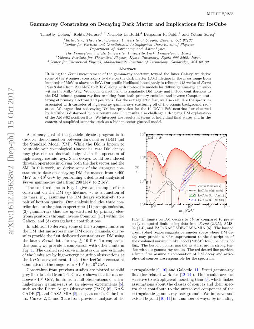
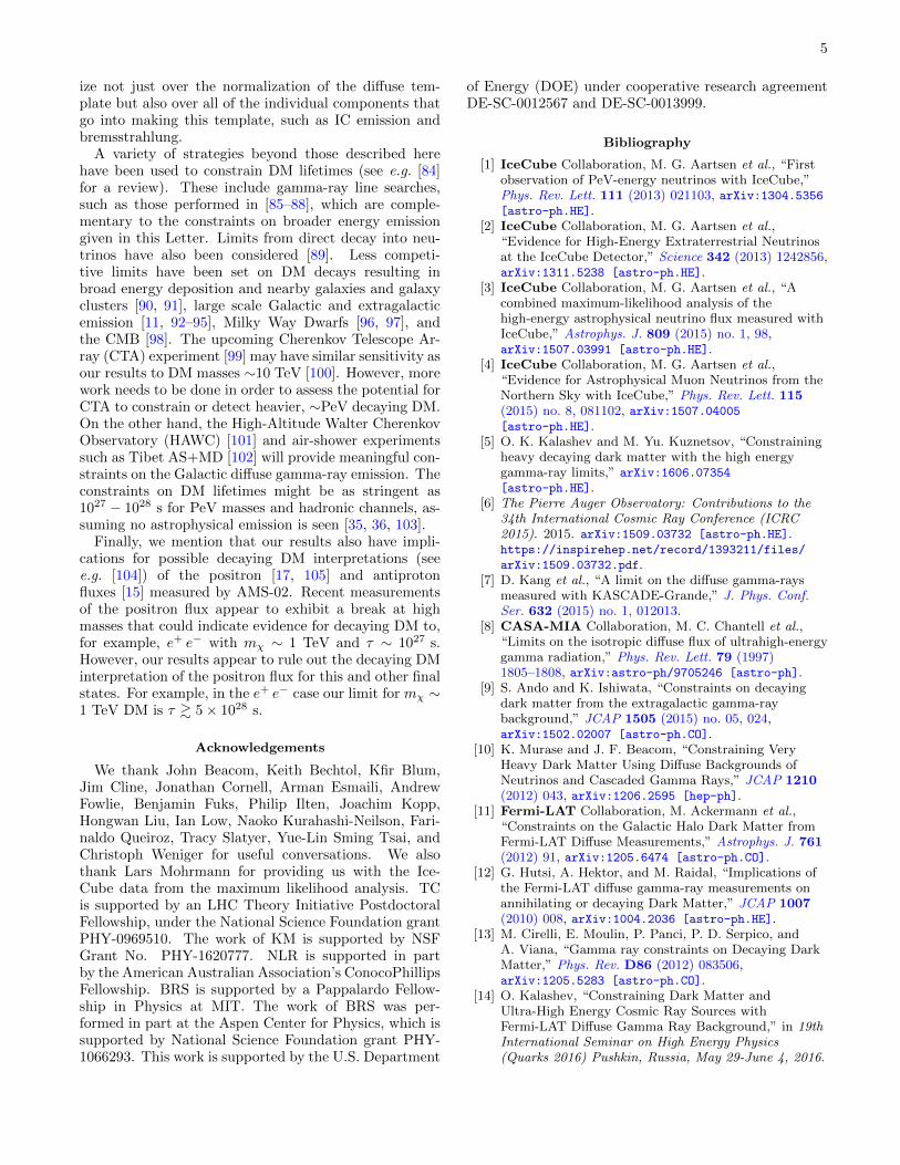
The solid red line in Fig. 1 gives an example of ourconstraint on the DM (χ) lifetime, τ , as a function ofits mass, mχ, assuming the DM decays exclusively to apair of bottom quarks. Our analysis includes three con-tributions to the photon spectrum: (1) prompt emission,(2) gamma-rays that are up-scattered by primary elec-trons/positrons through inverse Compton (IC) within theGalaxy, and (3) extragalactic contributions.

In addition to deriving some of the strongest limits onthe DM lifetime across many DM decay channels, our re-sults provide the first dedicated constraints on DM usingthe latest Fermi data for mχ & 10 TeV. To emphasizethis point, we provide a comparison with other limits inFig. 1. The dashed red curve indicates our new estimateof the limits set by high-energy neutrino observations atthe IceCube experiment [1–4]. Our IceCube constraintdominates in the range from ∼107 to 109 GeV.

Constraints from previous studies are plotted as solidgrey lines labeled from 1-6. Curve 6 shows that for massesabove ∼109 GeV, limits from null observations of ultra-high-energy gamma-rays at air shower experiments [5],such as the Pierre Auger Observatory (PAO) [6], KAS-CADE [7], and CASA-MIA [8], surpass our IceCube lim-its. Curves 2, 5, and 3 are from previous analyses of the

102 104 106 108 1010

mχ [GeV]

1026

1027

1028

1029

τ[s

]DM → bb

1

2

3

4

5

6

Fermi (this work)

IceCube (this work)

IceCube 3σ (Comb.)

IceCube 3σ (MESE)

FIG. 1: Limits on DM decays to b b, as compared to previ-ously computed limits using data from Fermi (2,3,5), AMS-02 (1,4), and PAO/KASCADE/CASA-MIA (6). The hashedgreen (blue) region suggests parameter space where DM de-cay may provide a ∼3σ improvement to the description ofthe combined maximum likelihood (MESE) IceCube neutrinoflux. The best-fit points, marked as stars, are in strong ten-sion with our gamma-ray results. The red dotted line providesa limit if we assume a combination of DM decay and astro-physical sources are responsible for the spectrum.

extragalactic [9, 10] and Galactic [11] Fermi gamma-rayflux (for related work see [12–14]). Our results are lesssensitive to astrophysical modeling than [9], which makesassumptions about the classes of sources and their spec-tra that contribute to the unresolved component of theextragalactic gamma-ray background. We improve andextend beyond [10, 11] in a number of ways: by including

arX

iv:1

612.

0563

8v2

[he

p-ph

] 1

5 O

ct 2

017

2

state-of-the-art modeling for cosmic-ray-induced gamma-ray emission in the Milky Way, a larger and cleaner dataset, and a novel analysis technique that allows us tosearch for a combination of Galactic and extragalacticflux arising from DM decay. The limits labeled 1 and 4in Fig. 1 are from the AMS-02 antiproton [15, 16] andpositron [17, 18] measurements, respectively; these con-straints are subject to considerable astrophysical uncer-tainties, due to the propagation of charged cosmic raysfrom their source to Earth.

An additional motivation for this work is the measure-ment of the so far unexplained high-energy neutrinos ob-served by the IceCube experiment [1–4]. If the DM hasboth a mass mχ ∼ PeV and a long lifetime τ ∼ 1028 sec-onds, its decays could contribute to the upper end of theIceCube spectrum. These DM candidates would producecorrelated cosmic-ray signals, yielding a broad spectrumof gamma rays with energies extending well into Fermi ’senergy range. Taking this correlation between neutrinoand photon spectra into account enables us to constrainthe DM interpretation of these neutrinos using the Fermidata.

Figure 1 illustrates regions of parameter space wherewe fit a decaying DM spectrum to the high-energy neu-trino flux at IceCube in hashed green. The correspondingregion for the analysis of Ref. [19] using lower-energy neu-trinos is shown in blue. Clearly, much of the parameterspace relevant for IceCube is disfavored by the gamma-ray limits; the best fit points (indicated by stars) are instrong tension with the Fermi observations. We concludethat models where decaying DM could account for theentire astrophysical neutrino flux observed by IceCubeare disfavored. Furthermore, models where the neutrinoflux results from a mix of decaying DM and astrophysicalsources are strongly constrained.

The rest of this Letter is organized as follows. First, wediscuss the various contributions to the gamma-ray fluxresulting from DM decay. Then, we give an overview ofthe data set and analysis techniques used in this work.Next, we provide context for these limits by interpretingthem as constraints on a concrete model (glueball DM),before concluding.

II. THE GAMMA-RAY FLUX

Decaying DM contributes both a Galactic and extra-galactic flux. The Galactic contribution results primarilyfrom prompt gamma-ray emission due to the decay itself,which is simulated with Pythia 8.219 [20–22] includingelectroweak showering [23] (see e.g. [24–34]).

These effects can be the only source of photons forchannels such as χ→ νν.

In addition, the electrons and positrons from thesedecays IC scatter off of cosmic background radiation(CBR), producing gamma-rays (see e.g. [35, 36]). Theprompt contribution follows the spatial morphology ob-tained from the line-of-sight (LOS) integral of theDM density, which we model with a Navarro-Frenk-White (NFW) profile [37, 38], setting the local DM den-

sity ρ = 0.3 GeV/cm3, and the scale radius rs = 20 kpc(variations to the profile lead to similar results, see theSupplementary Material). We only consider IC scatter-ing off of the cosmic microwave background (CMB), asscattering from integrated stellar radiation and the in-frared background is expected to be sub-dominant, seethe Supplementary Material. For scattering off of theCMB, the resulting gamma-ray morphology also followsthe LOS integral of the DM density. Importantly, as scat-tering off of the other radiation fields only increases thegamma-ray flux, neglecting these effects is conservative.In the same spirit, we conservatively assume that theelectrons and positrons lose energy due to synchrotronemission in a rather strong, uniform B = 2.0 µG mag-netic field (see e.g. [39–41]) and show variations in theSupplementary Material.

In addition to the Galactic fluxes, there is an essen-tially isotropic extragalactic contribution, arising fromDM decays throughout the broader Universe [42]. Theextragalactic flux receives three important contributions:(1) attenuated prompt emission; (2) attenuated emissionfrom IC of primary electrons and positrons; and (3) emis-sion from gamma-ray cascades. The cascade emissionarises when an electron-positron pair is created by high-energy gamma rays scattering off of the CBR, inducingIC emission along with adiabatic energy loss. We accountfor these effects following [10, 35].

III. DATA ANALYSIS

We assess how well predicted Galactic (NFW-correlated) and extragalactic (isotropic) fluxes de-scribe the data using the profile-likelihood method (seee.g. [43]), described in more detail in the SupplementaryMaterial. To this end, we perform a template fittinganalysis (using NPTFit [44]) with 413 weeks of FermiPass 8 data collected from August 4, 2008 to July 7,2016. We restrict to the UltracleanVeto event class;furthermore, we only use the top quartile of events asranked by point-spread function (PSF). The Ultraclean-Veto event class is used to minimize contamination fromcosmic rays, while the PSF cut is imposed to mitigateeffects from mis-modeling bright regions. We bin thedata in 40 logarithmically-spaced energy bins between200 MeV and 2 TeV, and we apply the recommendedquality cuts DATA QUAL>0 && LAT CONFIG==1 and zenithangle less than 90 [45]. The data is binned spatially us-ing a HEALPix [46] pixelation with nside=128.

We constrain this data to a region of interest (ROI)defined by Galactic latitude |b| ≥ 20 within 45 of theGalactic Center (GC). The Galactic plane is masked inorder to avoid issues related to mismodeling of diffuseemission in that region. Similarly, we do not extend ourregion out further from the GC to avoid over-subtractionissues that may arise when fitting diffuse templates overlarge regions of the sky (see e.g. [47–49]). Finally wemask all point sources (PSs) in the 3FGL PS catalog [50]at their 95% containment radius.

Using this restricted dataset, we then independently

3

fit templates in each energy bin in order to construct alikelihood profile as a function of the extragalactic andGalactic flux. We separate our model parameters intothose of interest ψ and the nuisance parameters λ. Theψ include parameters for an isotropic template to ac-count for the extragalactic emission, along with a tem-plate following a LOS-integrated NFW profile to modelthe Galactic emission. Note that both the prompt and ICcontribute to the same template, see the SupplementaryMaterial for justification. The λ include parameters forthe flux from diffuse emission within the Milky Way, fluxfrom the Fermi bubbles, flux from isotropic emission thatdoes not arise from DM decay (e.g. emission from blazarsand other extragalactic sources, along with misidentifiedcosmic rays), and flux from PSs, both Galactic and ex-tragalactic, in the 3FGL PS catalog. Importantly, eachspatial template is given a separate, uncorrelated degreeof freedom in the northern and southern hemispheres,further alleviating over-subtraction.

In our main analysis, we use the Pass 7 diffuse modelgal 2yearp7v6 v0 (p7v6) to account for diffuse emissionin the Milky Way, coming from gas-correlated emission(mostly pion decay and bremsstrahlung from high-energyelectrons), IC emission, and emission from large-scalestructures such as the Fermi bubbles [51] and Loop 1 [52].Additionally, even though the Fermi bubbles are includedto some extent in the p7v6 model, we add an additionaldegree of freedom for the bubbles, following the uniformspatial template given in [51]. We add a single templatefor all 3FGL PSs based on the spectra in [50], though weemphasize again that all PSs are masked at 95% contain-ment. See the Supplementary Material for variations ofthese choices.

Given the templates described above, weare able to construct 2-d log-likelihood profileslog pi(di|Iiiso, IiNFW) as functions of the isotropicand NFW-correlated DM-induced emission Iiiso andIiNFW, respectively, in each of the energy bins i. Here,di is the data in that energy bin, which simply consistsof the number of counts in each pixel. The likelihoodprofiles are given by maximizing the Poisson likelihoodfunctions over the λ parameters.

Any decaying DM model may be constrained fromthe set of likelihood profiles in each energy bin, whichare provided as Supplementary Data [53]. Con-cretely, given a DM model M, the total log-likelihoodlog p(d|M, τ,mχ) is simply the sum of the log pi, wherethe intensities in each energy bin are functions of the DMmass and lifetime. The test-statistics (TS) used to con-strain the model is twice the difference between the log-likelihood at a given τ and the value at τ = ∞, wherethe DM contributes no flux. The 95% limit is given byTS = −2.71.

In order to compare our gamma-ray results to poten-tial signals from IceCube, we determine the region of pa-rameter space where DM may contribute to the observedhigh-energy neutrino flux. We use the recent high-energyastrophysical neutrino spectrum measurement by the Ice-

Cube collaboration [3]. In that work, neutrino flux mea-surements from a combination of muon-track and showerdata are given in 9 logarithmically-spaced energy bins be-tween 10 TeV and 10 PeV, under the assumption of equalflavor ratios and an isotropic flux.1 We assume that DMdecays are the only source of high-energy neutrino flux.In Fig. 1 (assuming the DM decays exclusively to bb) weshow the region where the DM model provides at leasta 3σ improvement over the null hypothesis of no high-energy flux at all. The best-fit point is marked with astar. The blue region in Fig. 1 is the best-fit region [19]for explaining an apparent excess in the 2-year mediumenergy starting event (MESE) IceCube data, which ex-tends down to energies ∼1 TeV [55].

The dashed red curve, on other other hand, shows the95% limit that we obtain on this DM channel under theassumption that astrophysical sources also contribute tothe high-energy flux. We parameterize the astrophysicalflux by a power-law with an exponential cut-off, and wemarginalize over the slope of the power-law, the normal-ization, and the cut-off in order to obtain a likelihoodprofile for the DM model, as a function of τ and mχ.We emphasize that we allow the spectral index to float,as opposed to the analysis of [19], which fixes the indexequal to two.

IV. INTERPRETATIONS

In Fig. 1, we show our total constraint on the DMlifetime for a model where χ → b b. This result demon-strates tension in models where decaying DM explains orcontributes to the astrophysical neutrino flux observed byIceCube. PeV-scale decaying DM models have receivedattention recently (see e.g. [5, 35, 56–76]). In particular,while conventional astrophysical models such as those in-volving star-forming galaxies and galaxy clusters provideviable explanations for the neutrino data above 100 TeV(see [77] for a summary of recent ideas), the MESE datahave been difficult to explain with conventional mod-els [78, 79]. Moreover, it is natural to expect heavy DMto slowly decay to the SM in a wide class of scenarioswhere, for example, the DM is stabilized through globalsymmetries in a hidden sector that are expected to be vi-olated at the Planck scale or perhaps the scale of grandunification (the GUT scale).

From a purely data-driven point of view it is worth-while to ask whether any set of SM final states may con-tribute significantly to or explain the IceCube data whilebeing consistent with the gamma-ray constraints. In theSupplementary Material we provide limits on a variety oftwo-body SM final states.

It is also important to interpret the bounds as con-straints on the parameter space of UV models or gauge-

1 Constraints at high masses may be improved by incorporatingrecent results from [54], which focused on neutrino events withenergies greater than 10 PeV.

4

invariant effective field theory (EFT) realizations. If thedecay is mediated by irrelevant operators, and given thelong lifetimes we are probing, it is natural to assume veryhigh cut-off scales Λ, such as the GUT scale ∼1016 GeVor the Planck scale mPl ' 2.4× 1018 GeV. We expect allgauge invariant operators connecting the dark sector tothe SM to appear in the EFT suppressed by a scale mPl

or less (assuming no accidentally small coefficients and,perhaps, discrete global symmetries).

It is also interesting to consider models that could yieldsignals relevant for this analysis. Many cases are ex-plored in the Supplementary Material, and here we high-light one simple option: a hidden sector that consistsof a confining gauge theory, at scale ΛD [80], withoutadditional light matter. Hidden gauge sectors that de-couple from the SM at high scales appear to be genericin many string constructions (see [81] for a recent dis-cussion). Denoting the hidden-sector field strength asGDµν , then the lowest dimensional operator connectingthe hidden sector to the SM appears at dimension-6:L ⊃ λD GDµν G

µνD |H|2/Λ2, where λD is a dimension-

less coupling constant, Λ is the scale where this operatoris generated, and H the SM Higgs doublet. The light-est 0++ glueball state in the hidden gauge theory is asimple DM candidate χ, with mχ ∼ ΛD, though heav-ier, long-lived states may also play important roles (seee.g. [82]). The lowest dimension EFT operator connect-ing χ to the SM is then ∼ χ |H|2 Λ3

D/Λ2. Furthermore,

ΛD & 100 MeV in order to avoid constraints on DM self-interactions [83].

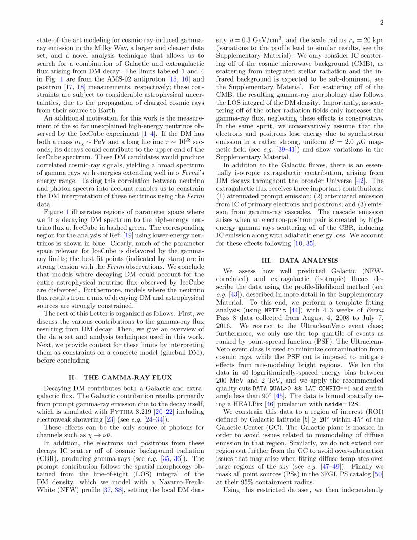
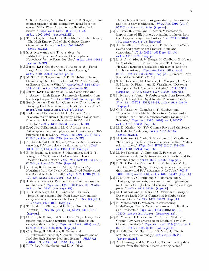
At masses comparable to and lower than the elec-troweak scale, the glueball decays primary to b quarksthrough mixing with the SM Higgs, while at high massesthe glueball decays predominantly to W±, Z0, and Higgsboson pairs (see the inset of Fig. 2 for the dominantbranching ratios). In the high-mass limit, the lifetimeis approximately

τ ' 5 · 1027 s

(3

ND

1

4πλD

)2(Λ

mPl

)4(0.1 PeV

ΛD

)5

, (1)

with ND the number of colors. This is roughly the rightlifetime to be relevant for the IceCube neutrino flux.

In Fig. 2, we show our constraint on this glueballmodel. Using Eq. (1), these results suggest that mod-els with ΛD & 0.1 PeV, λD & 1/(4π), and Λ = mPl areexcluded. As in Fig. 1, the shaded green is the region ofparameter space where the model may contribute signif-icantly to IceCube, and the dashed red line provides thelimit we obtain from IceCube allowing for an astrophysi-cal contribution to the flux. As in the case of the b b finalstate, the gamma-ray limits derived in this work are intension with the decaying-DM origin of the signal.

Figure 2 also illustrates the relative contribution ofprompt, IC and extragalactic emissions to the total limit.The 95% confidence interval is shown for each source, as-suming background templates only, where the normaliza-tions are fit to the data. Across almost all of the mass

102 104 106

mχ [GeV]

1024

1025

1026

1027

1028

τ[s

]

Glueball DM

EG only

IC only

Prompt only

Fermi combined

IceCube

102 104 106

mχ [GeV]

0.0

0.5

1.0

Bra

nch

ing

rati

os

hh

bb

ττ

WW + ZZ

FIG. 2: Limits on decaying glueball DM (see text for detals).We show limits obtained from prompt, IC, and EG emissiononly, along with the 95% confidence window for the expec-tation of each limit from MC simulations. Furthermore, theparameter space where the IceCube data may be interpretedas a ∼3σ hint for DM is shown in shaded green, with thebest fit point represented by the star. (inset) The dominantglueball DM branching ratios.

range, and particularly at the highest masses, the lim-its obtained on the real data align with the expectationsfrom MC. In the statistics-dominated regime, we wouldexpect the real-data limits to be consistent with thosefrom MC, while in the systematics dominated regime thelimits on real data may differ from those obtained fromMC. This is because the real data can have residuals com-ing from mis-modeling the background templates, andthe overall goodness of fit may increase with flux fromthe NFW-correlated template, for example, even in theabsence of DM. Alternatively, the background templatesmay overpredict the flux at certain regions of the sky,leading to over-subtraction issues that could make thelimits artificially strong.

V. DISCUSSION

In this work, we presented some of the strongest lim-its to date on decaying DM from a dedicated analysis ofFermi gamma-ray data incorporating spectral and spatialinformation, along with up-to-date modeling of diffuseemission in the Milky Way. Our results disfavor a decay-ing DM explanation of the IceCube high-energy neutrinodata.

There are several ways that our analysis could be ex-panded upon. We have not attempted to characterize thespectral composition of the astrophysical contributions tothe isotropic emission, which may strengthen our limits.On the other hand, ideally, for a given, fixed decayingDM flux in the profile likelihood, we should marginal-

5

ize not just over the normalization of the diffuse tem-plate but also over all of the individual components thatgo into making this template, such as IC emission andbremsstrahlung.

A variety of strategies beyond those described herehave been used to constrain DM lifetimes (see e.g. [84]for a review). These include gamma-ray line searches,such as those performed in [85–88], which are comple-mentary to the constraints on broader energy emissiongiven in this Letter. Limits from direct decay into neu-trinos have also been considered [89]. Less competi-tive limits have been set on DM decays resulting inbroad energy deposition and nearby galaxies and galaxyclusters [90, 91], large scale Galactic and extragalacticemission [11, 92–95], Milky Way Dwarfs [96, 97], andthe CMB [98]. The upcoming Cherenkov Telescope Ar-ray (CTA) experiment [99] may have similar sensitivity asour results to DM masses ∼10 TeV [100]. However, morework needs to be done in order to assess the potential forCTA to constrain or detect heavier, ∼PeV decaying DM.On the other hand, the High-Altitude Walter CherenkovObservatory (HAWC) [101] and air-shower experimentssuch as Tibet AS+MD [102] will provide meaningful con-straints on the Galactic diffuse gamma-ray emission. Theconstraints on DM lifetimes might be as stringent as1027 − 1028 s for PeV masses and hadronic channels, as-suming no astrophysical emission is seen [35, 36, 103].

Finally, we mention that our results also have impli-cations for possible decaying DM interpretations (seee.g. [104]) of the positron [17, 105] and antiprotonfluxes [15] measured by AMS-02. Recent measurementsof the positron flux appear to exhibit a break at highmasses that could indicate evidence for decaying DM to,for example, e+ e− with mχ ∼ 1 TeV and τ ∼ 1027 s.However, our results appear to rule out the decaying DMinterpretation of the positron flux for this and other finalstates. For example, in the e+ e− case our limit for mχ ∼1 TeV DM is τ & 5× 1028 s.

Acknowledgements

We thank John Beacom, Keith Bechtol, Kfir Blum,Jim Cline, Jonathan Cornell, Arman Esmaili, AndrewFowlie, Benjamin Fuks, Philip Ilten, Joachim Kopp,Hongwan Liu, Ian Low, Naoko Kurahashi-Neilson, Fari-naldo Queiroz, Tracy Slatyer, Yue-Lin Sming Tsai, andChristoph Weniger for useful conversations. We alsothank Lars Mohrmann for providing us with the Ice-Cube data from the maximum likelihood analysis. TCis supported by an LHC Theory Initiative PostdoctoralFellowship, under the National Science Foundation grantPHY-0969510. The work of KM is supported by NSFGrant No. PHY-1620777. NLR is supported in partby the American Australian Association’s ConocoPhillipsFellowship. BRS is supported by a Pappalardo Fellow-ship in Physics at MIT. The work of BRS was per-formed in part at the Aspen Center for Physics, which issupported by National Science Foundation grant PHY-1066293. This work is supported by the U.S. Department

of Energy (DOE) under cooperative research agreementDE-SC-0012567 and DE-SC-0013999.

Bibliography

[1] IceCube Collaboration, M. G. Aartsen et al., “Firstobservation of PeV-energy neutrinos with IceCube,”Phys. Rev. Lett. 111 (2013) 021103, arXiv:1304.5356[astro-ph.HE].

[2] IceCube Collaboration, M. G. Aartsen et al.,“Evidence for High-Energy Extraterrestrial Neutrinosat the IceCube Detector,” Science 342 (2013) 1242856,arXiv:1311.5238 [astro-ph.HE].

[3] IceCube Collaboration, M. G. Aartsen et al., “Acombined maximum-likelihood analysis of thehigh-energy astrophysical neutrino flux measured withIceCube,” Astrophys. J. 809 (2015) no. 1, 98,arXiv:1507.03991 [astro-ph.HE].

[4] IceCube Collaboration, M. G. Aartsen et al.,“Evidence for Astrophysical Muon Neutrinos from theNorthern Sky with IceCube,” Phys. Rev. Lett. 115(2015) no. 8, 081102, arXiv:1507.04005[astro-ph.HE].

[5] O. K. Kalashev and M. Yu. Kuznetsov, “Constrainingheavy decaying dark matter with the high energygamma-ray limits,” arXiv:1606.07354

[astro-ph.HE].[6] The Pierre Auger Observatory: Contributions to the

34th International Cosmic Ray Conference (ICRC2015). 2015. arXiv:1509.03732 [astro-ph.HE].https://inspirehep.net/record/1393211/files/

arXiv:1509.03732.pdf.[7] D. Kang et al., “A limit on the diffuse gamma-rays

measured with KASCADE-Grande,” J. Phys. Conf.Ser. 632 (2015) no. 1, 012013.

[8] CASA-MIA Collaboration, M. C. Chantell et al.,“Limits on the isotropic diffuse flux of ultrahigh-energygamma radiation,” Phys. Rev. Lett. 79 (1997)1805–1808, arXiv:astro-ph/9705246 [astro-ph].

[9] S. Ando and K. Ishiwata, “Constraints on decayingdark matter from the extragalactic gamma-raybackground,” JCAP 1505 (2015) no. 05, 024,arXiv:1502.02007 [astro-ph.CO].

[10] K. Murase and J. F. Beacom, “Constraining VeryHeavy Dark Matter Using Diffuse Backgrounds ofNeutrinos and Cascaded Gamma Rays,” JCAP 1210(2012) 043, arXiv:1206.2595 [hep-ph].

[11] Fermi-LAT Collaboration, M. Ackermann et al.,“Constraints on the Galactic Halo Dark Matter fromFermi-LAT Diffuse Measurements,” Astrophys. J. 761(2012) 91, arXiv:1205.6474 [astro-ph.CO].

[12] G. Hutsi, A. Hektor, and M. Raidal, “Implications ofthe Fermi-LAT diffuse gamma-ray measurements onannihilating or decaying Dark Matter,” JCAP 1007(2010) 008, arXiv:1004.2036 [astro-ph.HE].

[13] M. Cirelli, E. Moulin, P. Panci, P. D. Serpico, andA. Viana, “Gamma ray constraints on Decaying DarkMatter,” Phys. Rev. D86 (2012) 083506,arXiv:1205.5283 [astro-ph.CO].

[14] O. Kalashev, “Constraining Dark Matter andUltra-High Energy Cosmic Ray Sources withFermi-LAT Diffuse Gamma Ray Background,” in 19thInternational Seminar on High Energy Physics(Quarks 2016) Pushkin, Russia, May 29-June 4, 2016.

6

2016. arXiv:1608.07530 [astro-ph.HE].http://inspirehep.net/record/1484150/files/

arXiv:1608.07530.pdf.[15] Ams-02 Collaboration, talks at the ‘AMS Days at

CERN’, 2015, 15-17 april.[16] G. Giesen, M. Boudaud, Y. Genolini, V. Poulin,

M. Cirelli, P. Salati, and P. D. Serpico, “AMS-02antiprotons, at last!Secondary astrophysicalcomponent and immediate implications for DarkMatter,” JCAP 1509 (2015) no. 09, 023,arXiv:1504.04276 [astro-ph.HE].

[17] AMS Collaboration, M. Aguilar et al., “First Resultfrom the Alpha Magnetic Spectrometer on theInternational Space Station: Precision Measurement ofthe Positron Fraction in Primary Cosmic Rays of0.5–350 GeV,” Phys. Rev. Lett. 110 (2013) 141102.

[18] A. Ibarra, A. S. Lamperstorfer, and J. Silk, “Darkmatter annihilations and decays after the AMS-02positron measurements,” Phys. Rev. D89 (2014) no. 6,063539, arXiv:1309.2570 [hep-ph].

[19] M. Chianese, G. Miele, and S. Morisi, “Dark Matterinterpretation of low energy IceCube MESE excess,”arXiv:1610.04612 [hep-ph].

[20] T. Sjostrand, S. Mrenna, and P. Z. Skands, “PYTHIA6.4 Physics and Manual,” JHEP 05 (2006) 026,arXiv:hep-ph/0603175 [hep-ph].

[21] T. Sjostrand, S. Mrenna, and P. Z. Skands, “A BriefIntroduction to PYTHIA 8.1,” Comput.Phys.Commun.178 (2008) 852–867, arXiv:0710.3820 [hep-ph].

[22] T. Sjostrand, S. Ask, J. R. Christiansen, R. Corke,N. Desai, P. Ilten, S. Mrenna, S. Prestel, C. O.Rasmussen, and P. Z. Skands, “An Introduction toPYTHIA 8.2,” Comput. Phys. Commun. 191 (2015)159–177, arXiv:1410.3012 [hep-ph].

[23] J. R. Christiansen and T. Sjostrand, “Weak GaugeBoson Radiation in Parton Showers,” JHEP 04 (2014)115, arXiv:1401.5238 [hep-ph].

[24] M. Kachelriess and P. D. Serpico, “Model-independentdark matter annihilation bound from the diffuse γ rayflux,” Phys. Rev. D76 (2007) 063516,arXiv:0707.0209 [hep-ph].

[25] M. Regis and P. Ullio, “Multi-wavelength signals ofdark matter annihilations at the Galactic center,”Phys. Rev. D78 (2008) 043505, arXiv:0802.0234[hep-ph].

[26] G. D. Mack, T. D. Jacques, J. F. Beacom, N. F. Bell,and H. Yuksel, “Conservative Constraints on DarkMatter Annihilation into Gamma Rays,” Phys. Rev.D78 (2008) 063542, arXiv:0803.0157 [astro-ph].

[27] N. F. Bell, J. B. Dent, T. D. Jacques, and T. J. Weiler,“Electroweak Bremsstrahlung in Dark MatterAnnihilation,” Phys. Rev. D78 (2008) 083540,arXiv:0805.3423 [hep-ph].

[28] J. B. Dent, R. J. Scherrer, and T. J. Weiler, “Toward aMinimum Branching Fraction for Dark MatterAnnihilation into Electromagnetic Final States,” Phys.Rev. D78 (2008) 063509, arXiv:0806.0370[astro-ph].

[29] E. Borriello, A. Cuoco, and G. Miele, “Radioconstraints on dark matter annihilation in the galactichalo and its substructures,” Phys. Rev. D79 (2009)023518, arXiv:0809.2990 [astro-ph].

[30] G. Bertone, M. Cirelli, A. Strumia, and M. Taoso,“Gamma-ray and radio tests of the e+e- excess from

DM annihilations,” arXiv:0811.3744 [astro-ph].[31] N. F. Bell and T. D. Jacques, “Gamma-ray

Constraints on Dark Matter Annihilation into ChargedParticles,” arXiv:0811.0821 [astro-ph].

[32] M. Cirelli and P. Panci, “Inverse Compton constraintson the Dark Matter e+e- excesses,” Nucl. Phys. B821(2009) 399–416, arXiv:0904.3830 [astro-ph.CO].

[33] M. Kachelriess, P. D. Serpico, and M. A. Solberg, “Onthe role of electroweak bremsstrahlung for indirectdark matter signatures,” Phys. Rev. D80 (2009)123533, arXiv:0911.0001 [hep-ph].

[34] P. Ciafaloni, D. Comelli, A. Riotto, F. Sala,A. Strumia, and A. Urbano, “Weak Corrections areRelevant for Dark Matter Indirect Detection,” JCAP1103 (2011) 019, arXiv:1009.0224 [hep-ph].

[35] K. Murase, R. Laha, S. Ando, and M. Ahlers, “Testingthe Dark Matter Scenario for PeV Neutrinos Observedin IceCube,” Phys. Rev. Lett. 115 (2015) no. 7,071301, arXiv:1503.04663 [hep-ph].

[36] A. Esmaili and P. D. Serpico, “Gamma-ray boundsfrom EAS detectors and heavy decaying dark matterconstraints,” JCAP 1510 (2015) no. 10, 014,arXiv:1505.06486 [hep-ph].

[37] J. F. Navarro, C. S. Frenk, and S. D. M. White, “TheStructure of Cold Dark Matter Halos,” Astrophys. J.462 (1996) 563–575, astro-ph/9508025.

[38] J. F. Navarro, C. S. Frenk, and S. D. White, “AUniversal density profile from hierarchical clustering,”Astrophys.J. 490 (1997) 493–508,arXiv:astro-ph/9611107 [astro-ph].

[39] S. A. Mao, N. M. McClure-Griffiths, B. M. Gaensler,J. C. Brown, C. L. van Eck, M. Haverkorn, P. P.Kronberg, J. M. Stil, A. Shukurov, and A. R. Taylor,“New Constraints on the Galactic Halo Magnetic Fieldusing Rotation Measures of Extragalactic SourcesTowards the Outer Galaxy,” Astrophys. J. 755 (2012)21, arXiv:1206.3314 [astro-ph.GA].

[40] M. Haverkorn, “Magnetic Fields in the Milky Way,”arXiv:1406.0283 [astro-ph.GA].

[41] M. C. Beck, A. M. Beck, R. Beck, K. Dolag, A. W.Strong, and P. Nielaba, “New constraints on modellingthe random magnetic field of the MW,” JCAP 1605(2016) no. 05, 056, arXiv:1409.5120 [astro-ph.GA].

[42] G. D. Kribs and I. Z. Rothstein, “Bounds on longlivedrelics from diffuse gamma-ray observations,” Phys.Rev. D55 (1997) 4435–4449, arXiv:hep-ph/9610468[hep-ph]. [Erratum: Phys. Rev.D56,1822(1997)].

[43] W. A. Rolke, A. M. Lopez, and J. Conrad, “Limitsand confidence intervals in the presence of nuisanceparameters,” Nucl. Instrum. Meth. A551 (2005)493–503, arXiv:physics/0403059 [physics].

[44] S. Mishra-Sharma, N. L. Rodd, and B. R. Safdi,“NPTFit: A code package for Non-PoissonianTemplate Fitting,” arXiv:1612.03173 [astro-ph.HE].

[45] “http://fermi.gsfc.nasa.gov/ssc/data/analysis/documentation/cicerone/cicerone data exploration/data preparation.html.”.

[46] K. M. Gorski, E. Hivon, A. J. Banday, B. D. Wandelt,F. K. Hansen, M. Reinecke, and M. Bartelman,“HEALPix - A Framework for high resolutiondiscretization, and fast analysis of data distributed onthe sphere,” Astrophys. J. 622 (2005) 759–771,arXiv:astro-ph/0409513 [astro-ph].

[47] T. Daylan, D. P. Finkbeiner, D. Hooper, T. Linden,

7

S. K. N. Portillo, N. L. Rodd, and T. R. Slatyer, “Thecharacterization of the gamma-ray signal from thecentral Milky Way: A case for annihilating darkmatter,” Phys. Dark Univ. 12 (2016) 1–23,arXiv:1402.6703 [astro-ph.HE].

[48] T. Linden, N. L. Rodd, B. R. Safdi, and T. R. Slatyer,“The High-Energy Tail of the Galactic CenterGamma-Ray Excess,” arXiv:1604.01026

[astro-ph.HE].[49] S. A. Narayanan and T. R. Slatyer, “A

Latitude-Dependent Analysis of the LeptonicHypothesis for the Fermi Bubbles,” arXiv:1603.06582

[astro-ph.HE].[50] Fermi-LAT Collaboration, F. Acero et al., “Fermi

Large Area Telescope Third Source Catalog,”arXiv:1501.02003 [astro-ph.HE].

[51] M. Su, T. R. Slatyer, and D. P. Finkbeiner, “GiantGamma-ray Bubbles from Fermi-LAT: AGN Activityor Bipolar Galactic Wind?,” Astrophys.J. 724 (2010)1044–1082, arXiv:1005.5480 [astro-ph.HE].

[52] Fermi-LAT Collaboration, J.-M. Casandjian andI. Grenier, “High Energy Gamma-Ray Emission fromthe Loop I region,” arXiv:0912.3478 [astro-ph.HE].

[53] Supplementary Data for “Gamma-ray Constraints onDecaying Dark Matter and Implications for IceCube”.http://hdl.handle.net/1721.1/105550.

[54] IceCube Collaboration, M. G. Aartsen et al.,“Constraints on ultra-high-energy cosmic ray sourcesfrom a search for neutrinos above 10 PeV withIceCube,” arXiv:1607.05886 [astro-ph.HE].

[55] IceCube Collaboration, M. G. Aartsen et al.,“Atmospheric and astrophysical neutrinos above 1 TeVinteracting in IceCube,” Phys. Rev. D91 (2015) no. 2,022001, arXiv:1410.1749 [astro-ph.HE].

[56] A. Esmaili and P. D. Serpico, “Are IceCube neutrinosunveiling PeV-scale decaying dark matter?,” JCAP1311 (2013) 054, arXiv:1308.1105 [hep-ph].

[57] B. Feldstein, A. Kusenko, S. Matsumoto, and T. T.Yanagida, “Neutrinos at IceCube from HeavyDecaying Dark Matter,” Phys. Rev. D88 (2013) no. 1,015004, arXiv:1303.7320 [hep-ph].

[58] Y. Ema, R. Jinno, and T. Moroi, “Cosmic-RayNeutrinos from the Decay of Long-Lived Particle andthe Recent IceCube Result,” Phys. Lett. B733 (2014)120–125, arXiv:1312.3501 [hep-ph].

[59] J. Zavala, “Galactic PeV neutrinos from dark matterannihilation,” Phys. Rev. D89 (2014) no. 12, 123516,arXiv:1404.2932 [astro-ph.HE].

[60] A. Bhattacharya, M. H. Reno, and I. Sarcevic,“Reconciling neutrino flux from heavy dark matterdecay and recent events at IceCube,” JHEP 06 (2014)110, arXiv:1403.1862 [hep-ph].

[61] T. Higaki, R. Kitano, and R. Sato, “NeutrinofulUniverse,” JHEP 07 (2014) 044, arXiv:1405.0013[hep-ph].

[62] C. Rott, K. Kohri, and S. C. Park, “Superheavy darkmatter and IceCube neutrino signals: Bounds ondecaying dark matter,” Phys. Rev. D92 (2015) no. 2,023529, arXiv:1408.4575 [hep-ph].

[63] C. S. Fong, H. Minakata, B. Panes, andR. Zukanovich Funchal, “Possible Interpretations ofIceCube High-Energy Neutrino Events,” JHEP 02(2015) 189, arXiv:1411.5318 [hep-ph].

[64] E. Dudas, Y. Mambrini, and K. A. Olive,

“Monochromatic neutrinos generated by dark matterand the seesaw mechanism,” Phys. Rev. D91 (2015)075001, arXiv:1412.3459 [hep-ph].

[65] Y. Ema, R. Jinno, and T. Moroi, “CosmologicalImplications of High-Energy Neutrino Emission fromthe Decay of Long-Lived Particle,” JHEP 10 (2014)150, arXiv:1408.1745 [hep-ph].

[66] A. Esmaili, S. K. Kang, and P. D. Serpico, “IceCubeevents and decaying dark matter: hints andconstraints,” JCAP 1412 (2014) no. 12, 054,arXiv:1410.5979 [hep-ph].

[67] L. A. Anchordoqui, V. Barger, H. Goldberg, X. Huang,D. Marfatia, L. H. M. da Silva, and T. J. Weiler,“IceCube neutrinos, decaying dark matter, and theHubble constant,” Phys. Rev. D92 (2015) no. 6,061301, arXiv:1506.08788 [hep-ph]. [Erratum: Phys.Rev.D94,no.6,069901(2016)].

[68] S. M. Boucenna, M. Chianese, G. Mangano, G. Miele,S. Morisi, O. Pisanti, and E. Vitagliano, “DecayingLeptophilic Dark Matter at IceCube,” JCAP 1512(2015) no. 12, 055, arXiv:1507.01000 [hep-ph].

[69] P. Ko and Y. Tang, “IceCube Events from Heavy DMdecays through the Right-handed Neutrino Portal,”Phys. Lett. B751 (2015) 81–88, arXiv:1508.02500[hep-ph].

[70] C. El Aisati, M. Gustafsson, T. Hambye, andT. Scarna, “Dark Matter Decay to a Photon and aNeutrino: the Double Monochromatic Smoking GunScenario,” Phys. Rev. D93 (2016) no. 4, 043535,arXiv:1510.05008 [hep-ph].

[71] M. D. Kistler, “On TeV Gamma Rays and the Searchfor Galactic Neutrinos,” arXiv:1511.05199

[astro-ph.HE].[72] M. Chianese, G. Miele, S. Morisi, and E. Vitagliano,

“Low energy IceCube data and a possible Dark Matterrelated excess,” Phys. Lett. B757 (2016) 251–256,arXiv:1601.02934 [hep-ph].

[73] M. Re Fiorentin, V. Niro, and N. Fornengo, “Aconsistent model for leptogenesis, dark matter and theIceCube signal,” arXiv:1606.04445 [hep-ph].

[74] P. S. B. Dev, D. Kazanas, R. N. Mohapatra, V. L.Teplitz, and Y. Zhang, “Heavy right-handed neutrinodark matter and PeV neutrinos at IceCube,” JCAP1608 (2016) no. 08, 034, arXiv:1606.04517 [hep-ph].

[75] P. Di Bari, P. O. Ludl, and S. Palomares-Ruiz,“Unifying leptogenesis, dark matter and high-energyneutrinos with right-handed neutrino mixing via Higgsportal,” arXiv:1606.06238 [hep-ph].

[76] M. Chianese and A. Merle, “A Consistent Theory ofDecaying Dark Matter Connecting IceCube to theSesame Street,” arXiv:1607.05283 [hep-ph].

[77] K. Murase and E. Waxman, “ConstrainingHigh-Energy Cosmic Neutrino Sources: Implicationsand Prospects,” Phys. Rev. D94 (2016) no. 10,103006, arXiv:1607.01601 [astro-ph.HE].

[78] K. Murase, D. Guetta, and M. Ahlers, “HiddenCosmic-Ray Accelerators as an Origin of TeV-PeVCosmic Neutrinos,” Phys. Rev. Lett. 116 (2016) no. 7,071101, arXiv:1509.00805 [astro-ph.HE].

[79] A. Palladino, M. Spurio, and F. Vissani, “On theIceCube spectral anomaly,” arXiv:1610.07015

[astro-ph.HE].[80] A. E. Faraggi and M. Pospelov, “Selfinteracting dark

matter from the hidden heterotic string sector,”

8

Astropart. Phys. 16 (2002) 451–461,arXiv:hep-ph/0008223 [hep-ph].

[81] J. Halverson, B. D. Nelson, and F. Ruehle, “StringTheory and the Dark Glueball Problem,”arXiv:1609.02151 [hep-ph].

[82] L. Forestell, D. E. Morrissey, and K. Sigurdson,“Non-Abelian Dark Forces and the Relic Densities ofDark Glueballs,” arXiv:1605.08048 [hep-ph].

[83] K. K. Boddy, J. L. Feng, M. Kaplinghat, and T. M. P.Tait, “Self-Interacting Dark Matter from aNon-Abelian Hidden Sector,” Phys. Rev. D89 (2014)no. 11, 115017, arXiv:1402.3629 [hep-ph].

[84] A. Ibarra, D. Tran, and C. Weniger, “Indirect Searchesfor Decaying Dark Matter,” Int. J. Mod. Phys. A28(2013) 1330040, arXiv:1307.6434 [hep-ph].

[85] A. A. Abdo et al., “Fermi LAT Search for PhotonLines from 30 to 200 GeV and Dark MatterImplications,” Phys. Rev. Lett. 104 (2010) 091302,arXiv:1001.4836 [astro-ph.HE].

[86] G. Vertongen and C. Weniger, “Hunting Dark MatterGamma-Ray Lines with the Fermi LAT,” JCAP 1105(2011) 027, arXiv:1101.2610 [hep-ph].

[87] Fermi-LAT Collaboration, M. Ackermann et al.,“Fermi LAT Search for Dark Matter in Gamma-rayLines and the Inclusive Photon Spectrum,” Phys. Rev.D86 (2012) 022002, arXiv:1205.2739 [astro-ph.HE].

[88] Fermi-LAT Collaboration, M. Ackermann et al.,“Search for gamma-ray spectral lines with the Fermilarge area telescope and dark matter implications,”Phys. Rev. D88 (2013) 082002, arXiv:1305.5597[astro-ph.HE].

[89] A. Esmaili, A. Ibarra, and O. L. G. Peres, “Probingthe stability of superheavy dark matter particles withhigh-energy neutrinos,” JCAP 1211 (2012) 034,arXiv:1205.5281 [hep-ph].

[90] L. Dugger, T. E. Jeltema, and S. Profumo,“Constraints on Decaying Dark Matter from FermiObservations of Nearby Galaxies and Clusters,” JCAP1012 (2010) 015, arXiv:1009.5988 [astro-ph.HE].

[91] X. Huang, G. Vertongen, and C. Weniger, “ProbingDark Matter Decay and Annihilation with Fermi LATObservations of Nearby Galaxy Clusters,” JCAP 1201(2012) 042, arXiv:1110.1529 [hep-ph].

[92] M. Cirelli, P. Panci, and P. D. Serpico, “Diffusegamma ray constraints on annihilating or decayingDark Matter after Fermi,” Nucl. Phys. B840 (2010)284–303, arXiv:0912.0663 [astro-ph.CO].

[93] L. Zhang, C. Weniger, L. Maccione, J. Redondo, andG. Sigl, “Constraining Decaying Dark Matter withFermi LAT Gamma-rays,” JCAP 1006 (2010) 027,arXiv:0912.4504 [astro-ph.HE].

[94] Fermi-LAT Collaboration, G. Zaharijas, A. Cuoco,Z. Yang, and J. Conrad, “Constraints on the GalacticHalo Dark Matter from Fermi-LAT DiffuseMeasurements,” PoS IDM2010 (2011) 111,arXiv:1012.0588 [astro-ph.HE].

[95] Fermi-LAT Collaboration, G. Zaharijas, J. Conrad,A. Cuoco, and Z. Yang, “Fermi-LAT measurement ofthe diffuse gamma-ray emission and constraints on theGalactic Dark Matter signal,” Nucl. Phys. Proc. Suppl.239-240 (2013) 88–93, arXiv:1212.6755[astro-ph.HE].

[96] VERITAS Collaboration, E. Aliu et al., “VERITASDeep Observations of the Dwarf Spheroidal Galaxy

Segue 1,” Phys. Rev. D85 (2012) 062001,arXiv:1202.2144 [astro-ph.HE]. [Erratum: Phys.Rev.D91,no.12,129903(2015)].

[97] M. G. Baring, T. Ghosh, F. S. Queiroz, and K. Sinha,“New Limits on the Dark Matter Lifetime from DwarfSpheroidal Galaxies using Fermi-LAT,” Phys. Rev.D93 (2016) no. 10, 103009, arXiv:1510.00389[hep-ph].

[98] T. R. Slatyer and C.-L. Wu, “General Constraints onDark Matter Decay from the Cosmic MicrowaveBackground,” arXiv:1610.06933 [astro-ph.CO].

[99] CTA Consortium Collaboration, M. Actis et al.,“Design concepts for the Cherenkov Telescope ArrayCTA: An advanced facility for ground-basedhigh-energy gamma-ray astronomy,” Exper. Astron. 32(2011) 193–316, arXiv:1008.3703 [astro-ph.IM].

[100] M. Pierre, J. M. Siegal-Gaskins, and P. Scott,“Sensitivity of CTA to dark matter signals from theGalactic Center,” JCAP 1406 (2014) 024,arXiv:1401.7330 [astro-ph.HE]. [Erratum:JCAP1410,E01(2014)].

[101] A. U. Abeysekara et al., “Sensitivity of the HighAltitude Water Cherenkov Detector to Sources ofMulti-TeV Gamma Rays,” Astropart. Phys. 50-52(2013) 26–32, arXiv:1306.5800 [astro-ph.HE].

[102] T. K. Sako, K. Kawata, M. Ohnishi, A. Shiomi,M. Takita, and H. Tsuchiya, “Exploration of a 100 TeVgamma-ray northern sky using the Tibet air-showerarray combined with an underground water-Cherenkovmuon-detector array,” Astropart. Phys. 32 (2009)177–184, arXiv:0907.4589 [astro-ph.IM].

[103] M. Ahlers and K. Murase, “Probing the GalacticOrigin of the IceCube Excess with Gamma-Rays,”Phys. Rev. D90 (2014) no. 2, 023010,arXiv:1309.4077 [astro-ph.HE].

[104] H.-C. Cheng, W.-C. Huang, X. Huang, I. Low, Y.-L. S.Tsai, and Q. Yuan, “AMS-02 Positron Excess andIndirect Detection of Three-body Decaying DarkMatter,” arXiv:1608.06382 [hep-ph].

[105] S. Ting, “The First Five Years of the Alpha MagneticSpectrometer on the International Space Station. TheFirst Five Years of the Alpha Magnetic Spectrometeron the International Space Station,”.https://cds.cern.ch/record/2238506.

[106] M. Cirelli, G. Corcella, A. Hektor, G. Hutsi,M. Kadastik, P. Panci, M. Raidal, F. Sala, andA. Strumia, “PPPC 4 DM ID: A Poor ParticlePhysicist Cookbook for Dark Matter IndirectDetection,” JCAP 1103 (2011) 051, arXiv:1012.4515[hep-ph]. [Erratum: JCAP1210,E01(2012)].

[107] G. Elor, N. L. Rodd, and T. R. Slatyer, “Multistepcascade annihilations of dark matter and the GalacticCenter excess,” Phys. Rev. D91 (2015) 103531,arXiv:1503.01773 [hep-ph].

[108] G. Elor, N. L. Rodd, T. R. Slatyer, and W. Xue,“Model-Independent Indirect Detection Constraints onHidden Sector Dark Matter,” arXiv:1511.08787

[hep-ph].[109] Fermi-LAT Collaboration, M. Ackermann et al.,

“The spectrum of isotropic diffuse gamma-ray emissionbetween 100 MeV and 820 GeV,” Astrophys. J. 799(2015) 86, arXiv:1410.3696 [astro-ph.HE].

[110] S. A. Mao, N. M. McClure-Griffiths, B. M. Gaensler,J. C. Brown, C. L. van Eck, M. Haverkorn, P. P.

9

Kronberg, J. M. Stil, A. Shukurov, and A. R. Taylor,“New Constraints on the Galactic Halo Magnetic FieldUsing Rotation Measures of Extragalactic Sourcestoward the Outer Galaxy,”Astrophys. J. 755 (Aug.,2012) 21, arXiv:1206.3314.

[111] A. Burkert, “The Structure of dark matter halos indwarf galaxies,” IAU Symp. 171 (1996) 175,arXiv:astro-ph/9504041 [astro-ph]. [Astrophys.J.447,L25(1995)].

[112] F. Calore, I. Cholis, and C. Weniger, “Backgroundmodel systematics for the Fermi GeV excess,” JCAP1503 (2015) 038, arXiv:1409.0042 [astro-ph.CO].

[113] P. Bhattacharjee and G. Sigl, “Origin and propagationof extremely high-energy cosmic rays,” Phys. Rept.327 (2000) 109–247, arXiv:astro-ph/9811011[astro-ph].

[114] J. F. Gunion and H. E. Haber, “The CP conservingtwo Higgs doublet model: The Approach to thedecoupling limit,” Phys. Rev. D67 (2003) 075019,arXiv:hep-ph/0207010 [hep-ph].

[115] B. P. Kersevan and E. Richter-Was, “Improved phasespace treatment of massive multi-particle final states,”Eur. Phys. J. C39 (2005) 439–450,arXiv:hep-ph/0405248 [hep-ph].

[116] A. Arvanitaki, S. Dimopoulos, S. Dubovsky, P. W.Graham, R. Harnik, and S. Rajendran, “AstrophysicalProbes of Unification,” Phys. Rev. D79 (2009) 105022,arXiv:0812.2075 [hep-ph].

[117] A. Arvanitaki, S. Dimopoulos, S. Dubovsky, P. W.Graham, R. Harnik, and S. Rajendran, “DecayingDark Matter as a Probe of Unification and TeVSpectroscopy,” Phys. Rev. D80 (2009) 055011,arXiv:0904.2789 [hep-ph].

[118] S. B. Roland, B. Shakya, and J. D. Wells, “NeutrinoMasses and Sterile Neutrino Dark Matter from thePeV Scale,” Phys. Rev. D92 (2015) no. 11, 113009,arXiv:1412.4791 [hep-ph].

[119] S. Cassel, D. M. Ghilencea, and G. G. Ross,“Electroweak and Dark Matter Constraints on aZ-prime in Models with a Hidden Valley,” Nucl. Phys.B827 (2010) 256–280, arXiv:0903.1118 [hep-ph].

[120] J. M. Cline, G. Dupuis, Z. Liu, and W. Xue, “Thewindows for kinetically mixed Z’-mediated dark matterand the galactic center gamma ray excess,” JHEP 08(2014) 131, arXiv:1405.7691 [hep-ph].

[121] K. Ishiwata, S. Matsumoto, and T. Moroi, “HighEnergy Cosmic Rays from the Decay of GravitinoDark Matter,” Phys. Rev. D78 (2008) 063505,arXiv:0805.1133 [hep-ph].

[122] M. Grefe, Neutrino signals from gravitino dark matterwith broken R-parity. PhD thesis, Hamburg U., 2008.arXiv:1111.6041 [hep-ph]. http://www-library.

desy.de/cgi-bin/showprep.pl?thesis08-043.[123] “FeynRules 2.0 - A complete toolbox for tree-level

phenomenology,” Comput. Phys. Commun. 185 (2014)2250–2300, arXiv:1310.1921 [hep-ph].

[124] J. Alwall, M. Herquet, F. Maltoni, O. Mattelaer, andT. Stelzer, “MadGraph 5 : Going Beyond,” JHEP 06(2011) 128, arXiv:1106.0522 [hep-ph].

[125] J. Alwall, R. Frederix, S. Frixione, V. Hirschi,F. Maltoni, O. Mattelaer, H. S. Shao, T. Stelzer,P. Torrielli, and M. Zaro, “The automatedcomputation of tree-level and next-to-leading orderdifferential cross sections, and their matching to

parton shower simulations,” JHEP 07 (2014) 079,arXiv:1405.0301 [hep-ph].

1

Gamma-ray Constraints on Decaying Dark Matter and Implications for IceCube

Supplementary Material

Timothy Cohen, Kohta Murase, Nicholas L. Rodd, Benjamin R. Safdi, and Yotam Soreq

The supplementary material is organized as follows. In Sec. I, we provide more detail regarding the methods usedin the main body of this work. In particular, we discuss the calculations of the gamma-ray spectra and the dataanalysis. In Sec. II, we give extended results beyond those given in the main body. Then, in Sec. III, we characterizeand test sources of systematic uncertainty that could affect our results. Lastly, in Sec. IV, we overview EFTs fordecaying DM and give constraints on explicit models beyond those discussed in the main text.

I. METHODS

We begin this section by detailing the calculations of the prompt and secondary spectra from DM decay. Then, wediscuss in detail the likelihood profile technique used in this paper.

A. Spectra

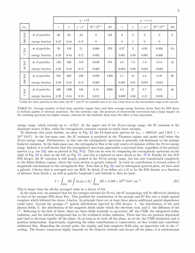
This section provides a more detailed description of the gamma-ray spectra that result from heavy DM decay.There is a natural decomposition into three components: (1) prompt Galactic gamma-ray emission, (2) Galacticinverse Compton (IC) emission from high-energy electrons and positrons up-scattering background photons, and(3) extragalactic flux from DM decay outside of our Galaxy. As mentioned in the main text, when calculatingthe prompt spectrum (and the primary electron and positron flux) it is crucial, for certain final states, to includedelectroweak radiative processes, as these may be the only source of gamma-ray emission. To illustrate this point,in Tab. S1 we show the average number of primary gamma-rays, neutrinos, and electrons and their energy fractioncoming from DM decay to b b and ν ν for various DM masses. We note that for mχ = 100 GeV there are in average3 (0) hadrons in the final state, while for mχ = 1 PeV there are 77 (1) hadrons for the bb (νeνe) decay mode. Theenergy fraction of these hadrons is 13 (0) % and 16 (0.5) % for bb (νeνe) modes with a DM mass of 100 GeV and 1 PeV,respectively. In addition, the energy fractions of photons, neutrinos and electrons are almost independent of the DMmass for the bb decay mode. This can be understood as the majority of these final states originate from pion decays.

Additionally, we show the typical number of radiated W and Z bosons. In the bb case, electroweak corrections arenot significant even for 1 PeV DM. However, in the νν case the radiated W and Z bosons are responsible for themajority of the primary particles (and all of the gamma-rays and electrons) at masses above the electroweak scale.The importance of these electroweak corrections on dark matter annihilation/decay spectra have been previouslynoted (see e.g. [24–34]). For DM masses above 10 PeV, the large number of final states implies that generation of thespectra through showering in Pythia is no longer practical. We discuss in Appendix IV B how we extend our spectrabeyond these masses.2

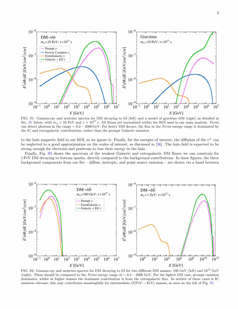
As was shown in Fig. 2 in the main text, the prompt flux tends to be most important for lower DM masses nearthe Fermi energy range, while the IC emission may play a leading role for DM masses near the PeV scale. Theextragalactic flux is important over the whole mass range, but at very high masses – well above the PeV scale – theextragalactic flux may be the only source of gamma-rays in the Fermi energy range. To illustrate these points, Fig. S1shows the gamma-ray and neutrino spectra at Earth, normalized to within the ROI used in our main analysis, for10 PeV DM decay with τ = 1027 s. We consider two final states, b b (left) and the gravitino model (right), which isdescribed in more detail later in this Supplementary Material.

Importantly, for DM masses &1 TeV, the gravitino decays roughly 50% of the time into W± `∓, where `∓ are SMleptons, and 50% of the time into Z0 ν and h ν. These latter two final states are responsible for the sharp rise in theGalactic and extragalactic neutrino spectrum in the gravitino model at energies approaching the DM mass (10 PeVin this case). In both cases, however, the prompt gamma-ray spectra are seen to be sub-dominant within the Fermi

2 Publicly available DM spectra, such as those in [106–108], do not extend up to these high masses, which is why we have recalculatedthem. While there are certainly modeling errors associated with running Pythia at these very high energies, they are expected tobe subdominant to the astrophysical uncertainties inherent in this analysis. We extend the spectra above 10 PeV by rescaling theappropriately normalized spectrum, as described and validated in the Supplementary Material.

2

χ→ b b χ→ νe νe

mχ γ ν e−/e+ W±/Z0 a All γ ν e−/e+ W±/Z0 a All100

GeV # of particles 26 66 23 0 120 0 2 0 0 2

energy fraction 0.27 0.44 0.17 0 - 0 1 0 0 -

1T

eV

# of particles 58 150 51 0.006 270 0.37 3 0.36 0.026 3.8

energy fraction 0.28 0.44 0.17 0.002 - 0.001 0.99 0.007 0.006 -

10

TeV # of particles 120 320 110 0.039 570 2.0 7.4 1.9 0.14 12

energy fraction 0.28 0.44 0.17 0.006 - 0.004 0.96 0.034 0.020 -

100

TeV # of particles 250 660 230 0.098 1200 5.1 15 4.8 0.35 26

energy fraction 0.29 0.44 0.17 0.009 - 0.007 0.91 0.078 0.033 -

1P

eV

# of particles 490 1300 440 0.18 2300 9.2 27 8.7 0.64 46

energy fraction 0.29 0.44 0.18 0.013 - 0.009 0.86 0.13 0.045 -

aUnlike the other particles in this table, the W± and Z0 are unstable and so we only count them at the intermediate stage of the cascade.

TABLE S1: Average number of final state particles (upper line) and their average energy fraction (lower line) for DM decayto bottom quarks or electron neutrinos. For the neutrino case, the presence of electroweak corrections has a large impact onthe resulting spectrum for higher masses, whereas for the hadronic final state the effect is less important.

energy range, which extends up to ∼2 TeV. At the upper end of the Fermi energy range, the IC emission is thedominant source of flux, while the extragalactic emission extends to much lower energies.

To illustrate this point further, we show in Fig. S2 the b b final-state spectra for mχ = 100 GeV and 1 ZeV(

=

1012 GeV). In the low-mass case, the IC emission is produced in the Thomson regime and peaks well below the

Fermi energy range. Furthermore, in this case the extragalactic spectrum is generally sub-dominant to the promptGalactic emission. In the high-mass case, the extragalactic flux is the only source of emission within the Fermi energyrange. Indeed, it is well known that the extragalactic spectrum approaches a universal form, regardless of the primaryspectra (e.g. see [10]; also as plotted in Fig. S12). This can be seen by comparing the extragalactic spectrum on theright of Fig. S2 to that on the left on Fig. S1, and this is explored in more detail in Sec. IV B. Finally for the ZeVDM decays, the IC emission is still largely peaked in the Fermi energy range, but has now transitioned completelyto the Klein-Nishina regime, where the cross section is greatly reduced. As such its contribution is several orders ofmagnitude sub-dominat to the extragalactic flux. Note that in Fig. S2, and in subsequent spectral plots, we have useda galactic J-factor that is averaged over our ROI. In detail, if we define ρ(s, l, b) to be the DM density as a functionof distance from Earth s, as well as galactic longitude l and latitude b, then we used:

J =

∫ROI

dΩ

∫ds ρ(s, l, b)/

∫ROI

dΩ ' 4.108× 1022 GeV cm−2 . (S1)

This is larger than the all-sky averaged value by a factor of 2.6.In the main text, we assumed that for the energies relevant for Fermi, the IC morphology will be effectively identical

to that of the prompt DM decay flux. This justified the combination of the prompt and IC flux into a single spatialtemplate which followed the above J-factor. In principle there are at least three places additional spatial dependencecould enter, beyond the prompt e± spatial distribution injected by DM decays: 1. the distribution of the seedphoton fields; 2. the distribution of the magnetic fields under which the electrons cool; and 3. the diffusion of thee±. Referring to the first of these, there are three fields available to up-scatter off: the CMB, the integrated stellarradiation, and the infrared background due to the irradiated stellar radiation. These last two are position dependentand tend to decrease rapidly off the plane. So as long as we look off the plane, as we do, the CMB dominates and isposition independent. Importantly, neglecting the other contributions is conservative, as they would only contributeadditional flux. Regarding the second point, the regular and halo magnetic fields play an important role in the e±

cooling. The former component highly depends on the Galactic latitude and decays off the plane; it is subdominant

3

10-1 100 101 102 103 104 105 106 10710-9

10-8

10-7

10-6

[]

Φ

/[

///]

→χ= τ=

γ

γ γ + ν

10-1 100 101 102 103 104 105 106 10710-9

10-8

10-7

10-6

[]

Φ

/[

///]

χ= τ=

FIG. S1: Gamma-ray and neutrino spectra for DM decaying to b b (left) and a model of gravitino DM (right) as detailed inSec. IV below, with mχ = 10 PeV and τ = 1027 s. All fluxes are normalized within the ROI used in our main analysis. Fermican detect photons in the range ∼ 0.2− 2000 GeV. For heavy DM decays, the flux in the Fermi energy range is dominated bythe IC and extragalactic contributions, rather than the prompt Galactic emission.

to the halo magnetic field in our ROI, so we ignore it. Finally, for the energies of interest, the diffusion of the e± canbe neglected to a good approximation on the scales of interest, as discussed in [36]. The halo field is expected to bestrong enough for electrons and positrons to lose their energy in the halo.

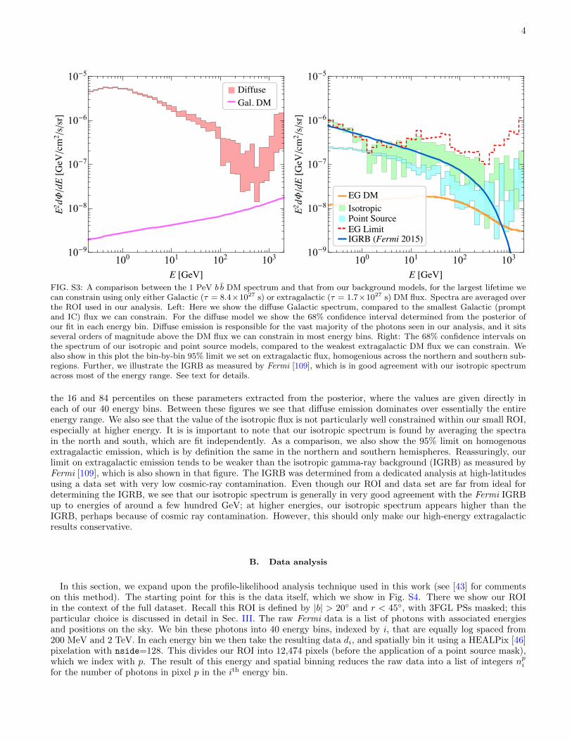
Finally, Fig. S3 shows the spectrum of the weakest Galactic and extragalactic DM fluxes we can constrain for1 PeV DM decaying to bottom quarks, directly compared to the background contributions. In these figures, the threebackground components from our fits – diffuse, isotropic, and point source emission – are shown via a band between

10-1 100 101 102 103 104 105 106 10710-9

10-8

10-7

10-6

[]

Φ

/[

///]

→χ= τ=

γ

γ + ν

100 102 104 106 108 1010 101210-9

10-8

10-7

10-6

[]

Φ

/[

///]

→χ= τ=

FIG. S2: Gamma-ray and neutrino spectra for DM decaying to b b for two different DM masses: 100 GeV (left) and 1012 GeV(right). These should be compared to the Fermi energy range of ∼ 0.2− 2000 GeV. For the lighter DM case, prompt emissiondominates, whilst at higher masses the dominant contribution is from the extragalactic flux. In neither of these cases is ICemission relevant, this only contributes meaningfully for intermediate O(PeV − EeV) masses, as seen on the left of Fig. S1.

4

100 101 102 10310-9

10-8

10-7

10-6

10-5

[]

Φ

/[

///]

100 101 102 10310-9

10-8

10-7

10-6

10-5

[]

Φ

/[

///]

( )

FIG. S3: A comparison between the 1 PeV b b DM spectrum and that from our background models, for the largest lifetime wecan constrain using only either Galactic (τ = 8.4×1027 s) or extragalactic (τ = 1.7×1027 s) DM flux. Spectra are averaged overthe ROI used in our analysis. Left: Here we show the diffuse Galactic spectrum, compared to the smallest Galactic (promptand IC) flux we can constrain. For the diffuse model we show the 68% confidence interval determined from the posterior ofour fit in each energy bin. Diffuse emission is responsible for the vast majority of the photons seen in our analysis, and it sitsseveral orders of magnitude above the DM flux we can constrain in most energy bins. Right: The 68% confidence intervals onthe spectrum of our isotropic and point source models, compared to the weakest extragalactic DM flux we can constrain. Wealso show in this plot the bin-by-bin 95% limit we set on extragalactic flux, homogenious across the northern and southern sub-regions. Further, we illustrate the IGRB as measured by Fermi [109], which is in good agreement with our isotropic spectrumacross most of the energy range. See text for details.

the 16 and 84 percentiles on these parameters extracted from the posterior, where the values are given directly ineach of our 40 energy bins. Between these figures we see that diffuse emission dominates over essentially the entireenergy range. We also see that the value of the isotropic flux is not particularly well constrained within our small ROI,especially at higher energy. It is is important to note that our isotropic spectrum is found by averaging the spectrain the north and south, which are fit independently. As a comparison, we also show the 95% limit on homogenousextragalactic emission, which is by definition the same in the northern and southern hemispheres. Reassuringly, ourlimit on extragalactic emission tends to be weaker than the isotropic gamma-ray background (IGRB) as measured byFermi [109], which is also shown in that figure. The IGRB was determined from a dedicated analysis at high-latitudesusing a data set with very low cosmic-ray contamination. Even though our ROI and data set are far from ideal fordetermining the IGRB, we see that our isotropic spectrum is generally in very good agreement with the Fermi IGRBup to energies of around a few hundred GeV; at higher energies, our isotropic spectrum appears higher than theIGRB, perhaps because of cosmic ray contamination. However, this should only make our high-energy extragalacticresults conservative.

B. Data analysis

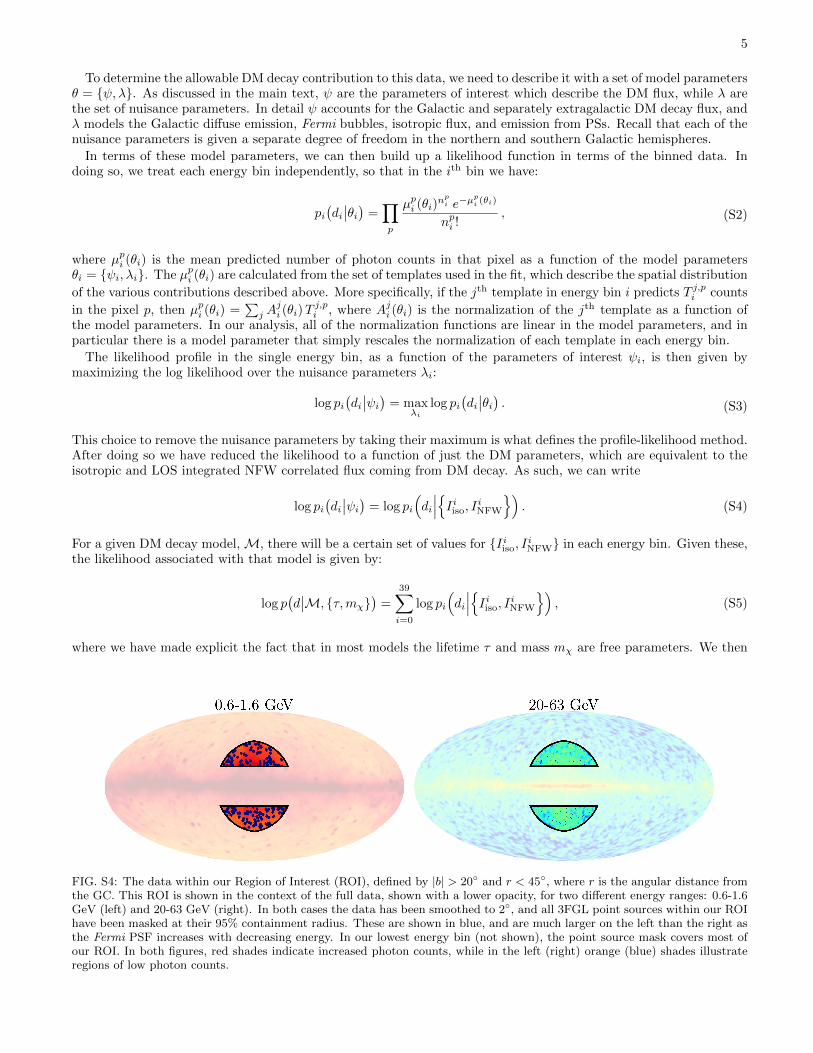
In this section, we expand upon the profile-likelihood analysis technique used in this work (see [43] for commentson this method). The starting point for this is the data itself, which we show in Fig. S4. There we show our ROIin the context of the full dataset. Recall this ROI is defined by |b| > 20 and r < 45, with 3FGL PSs masked; thisparticular choice is discussed in detail in Sec. III. The raw Fermi data is a list of photons with associated energiesand positions on the sky. We bin these photons into 40 energy bins, indexed by i, that are equally log spaced from200 MeV and 2 TeV. In each energy bin we then take the resulting data di, and spatially bin it using a HEALPix [46]pixelation with nside=128. This divides our ROI into 12,474 pixels (before the application of a point source mask),which we index with p. The result of this energy and spatial binning reduces the raw data into a list of integers npifor the number of photons in pixel p in the ith energy bin.

5

To determine the allowable DM decay contribution to this data, we need to describe it with a set of model parametersθ = ψ, λ. As discussed in the main text, ψ are the parameters of interest which describe the DM flux, while λ arethe set of nuisance parameters. In detail ψ accounts for the Galactic and separately extragalactic DM decay flux, andλ models the Galactic diffuse emission, Fermi bubbles, isotropic flux, and emission from PSs. Recall that each of thenuisance parameters is given a separate degree of freedom in the northern and southern Galactic hemispheres.

In terms of these model parameters, we can then build up a likelihood function in terms of the binned data. Indoing so, we treat each energy bin independently, so that in the ith bin we have:

pi(di∣∣θi) =

∏p

µpi (θi)npi e−µ

pi (θi)

npi !, (S2)

where µpi (θi) is the mean predicted number of photon counts in that pixel as a function of the model parametersθi = ψi, λi. The µpi (θi) are calculated from the set of templates used in the fit, which describe the spatial distribution

of the various contributions described above. More specifically, if the jth template in energy bin i predicts T j,pi counts

in the pixel p, then µpi (θi) =∑j A

ji (θi)T

j,pi , where Aji (θi) is the normalization of the jth template as a function of

the model parameters. In our analysis, all of the normalization functions are linear in the model parameters, and inparticular there is a model parameter that simply rescales the normalization of each template in each energy bin.

The likelihood profile in the single energy bin, as a function of the parameters of interest ψi, is then given bymaximizing the log likelihood over the nuisance parameters λi:

log pi(di∣∣ψi) = max

λilog pi

(di∣∣θi) . (S3)

This choice to remove the nuisance parameters by taking their maximum is what defines the profile-likelihood method.After doing so we have reduced the likelihood to a function of just the DM parameters, which are equivalent to theisotropic and LOS integrated NFW correlated flux coming from DM decay. As such, we can write

log pi(di∣∣ψi) = log pi

(di

∣∣∣Iiiso, IiNFW

). (S4)

For a given DM decay model,M, there will be a certain set of values for Iiiso, IiNFW in each energy bin. Given these,the likelihood associated with that model is given by:

log p(d∣∣M, τ,mχ

)=

39∑i=0

log pi

(di

∣∣∣Iiiso, IiNFW

), (S5)

where we have made explicit the fact that in most models the lifetime τ and mass mχ are free parameters. We then

FIG. S4: The data within our Region of Interest (ROI), defined by |b| > 20 and r < 45, where r is the angular distance fromthe GC. This ROI is shown in the context of the full data, shown with a lower opacity, for two different energy ranges: 0.6-1.6GeV (left) and 20-63 GeV (right). In both cases the data has been smoothed to 2, and all 3FGL point sources within our ROIhave been masked at their 95% containment radius. These are shown in blue, and are much larger on the left than the right asthe Fermi PSF increases with decreasing energy. In our lowest energy bin (not shown), the point source mask covers most ofour ROI. In both figures, red shades indicate increased photon counts, while in the left (right) orange (blue) shades illustrateregions of low photon counts.

6

define the test statistic (TS) used to constrain the model M by3

TS(M, τ,mχ

)= 2×

[log p

(d∣∣M, τ,mχ

)− log p

(d∣∣M, τ =∞,mχ

)]. (S6)

Note that fundamentally it is the list of values Iiiso, IiNFW that determine the TS. This means we can build a 2-dtable of TS values in each energy bin as a function of the extragalactic and Galactic DM flux. This table only needsto be computed once; afterwards a given model can be mapped onto a set of flux values, which has an associated TSin the tables. This is the approach we have followed, and we show these DM flux versus TS functions in Sec. II. Thetable of TS values is also available as Supplementary Data [53].

II. LIKELIHOOD PROFILES

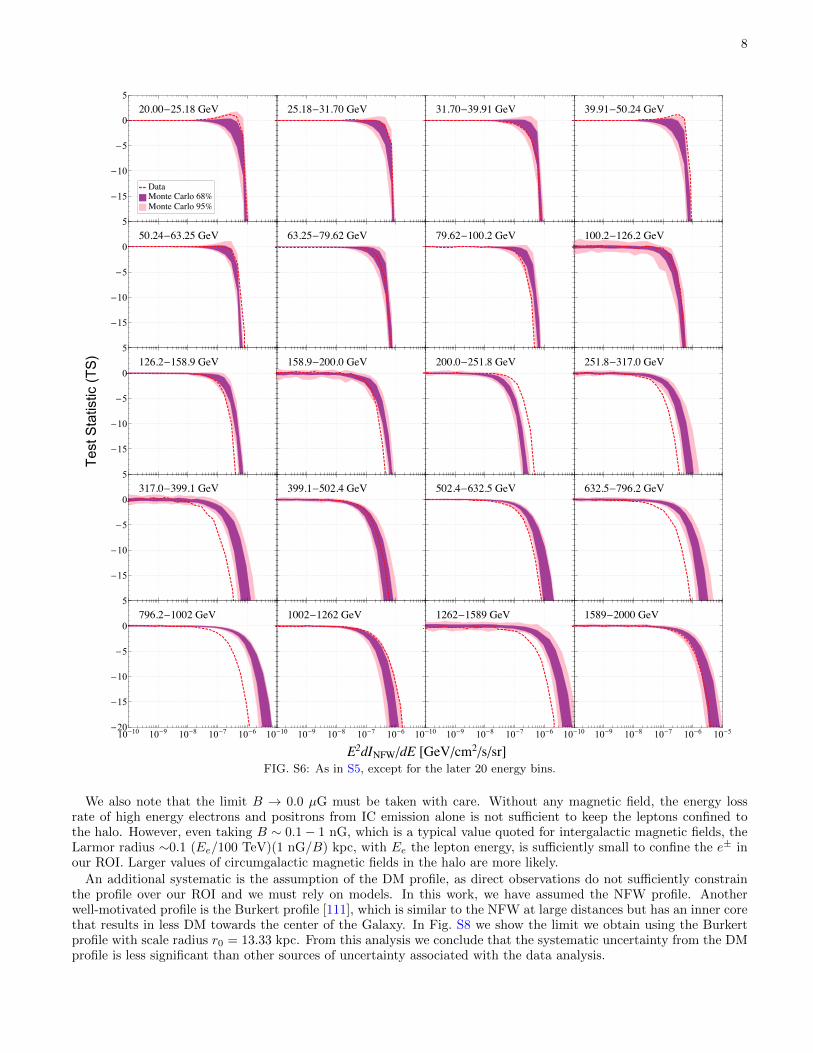
As described in the main text, our limits on specific DM final states and models are obtained from 2-d likelihoodprofiles, where the two dimensions encompass LOS integrated NFW correlated Galactic gamma-ray flux and extra-galactic gamma-ray flux. In Figs. S5 and S6 we show slices of these log-likelihood profiles when the extragalacticDM-induced flux is set to zero. The bands indicate the 68% and 95% confidence intervals for the expected profilesobtained from background-only MC simulations. The simulations use the set of background (“nuisance”) templatesnormalized to the best-fit values obtained from a template analysis of the data in the given energy bin. In mostenergy bins, the results obtained on the real data are consistent with the MC expectations, showing that – for themost part – we are in a statistics-dominated regime. In some energy bins, such as that from 15.9–20.0 GeV, the datashows a small excess in the TS compared to the MC expectation. While such an excess is perhaps not surprisingsince we are looking at multiple independent energy bins, it could also arise from a systematic discrepancy betweenthe background templates and the real data. More of a concern are energy bins where the limits set from the realdata are more constraining than the MC expectation, such as the energy bin from 0.5–0.63 GeV. It is possible thatthis discrepancy, in part, arises from an over-subtraction of diffuse emission in certain regions of sky since the diffusetemplate is not a perfect match for the real cosmic-ray induced emission in our Galaxy. This possibility – and theefforts that we have taken to minimize its impact—is discussed further in Sec. III.

In Fig. S7, we show a selection of the log-likelihood profiles found for vanishing Galactic DM-induced gamma-rayflux and shown instead as functions of the extragalactic DM-induced flux. It is important to remember that in thetemplate fit we marginalize over isotropic emission. As a result, it is impossible with our method to find a positivechange in the TS as we increase the DM-induced isotropic flux Iiso. In words, we remain completely agnostic towardsthe origin of the IGRB in our analysis. That is, we do not assume the IGRB is due to standard astrophysical emissionbut we also do not assume it is due to DM decay. The 1-d likelihood profiles as functions of Iiso instead show thelimits obtained for the isotropic flux coming simply from the requirement that they do not overproduce the observeddata.

In some energy bins, particularly at high energies (such as the energy bin from 632-796 GeV in Fig. S7), the datais seen to be more constraining than the MC expectation. However, we stress that the isotropic flux is not welldetermined, especially at these high energies, in our small region. With that said, the isotropic flux determined in thissmall region tends to be larger than the IGRB determined from a dedicated analysis at high latitudes (see Fig. S3).As a result, our limits on the extragalactic flux are likely conservative.

The full 2-d likelihood profiles are available as Supplementary Data [53]. These are given as a function of theaverage Galactic and extragalactic DM flux in our ROI, without including any point source mask. The absence of thepoint source mask is chosen to simplify the use of our flux-TS tables.

III. SYSTEMATICS TESTS

We have performed a variety of systematic tests to understand the robustness of our analysis. Figure S8 summarizesthe results of some of the more important tests.

In Fig. S8, we show limits on the b b final state with a variety of different variations on the analysis method. Certainvariations are shown to cause very little difference, such as not including an extra Fermi bubbles template, taking

3 Note that this TS stands in contrast to that used in [11]; in that work, the TS was similarly defined, except that instead of using τ =∞as a reference the τ of maximal likelihood was used. The definition of TS used here is more conservative than that in [11], thoughformally, with Wilk’s theorem in mind, our limits do not have the interpretation of 95% constraints.

7

B = 0.0 µG when computing the IC flux, and using the more up-to-date Pass 8 model gll iem v06 (p8r2) diffusemodel instead of the p7v6 model. As the p8r2 model identifies regions of extended excess emission in the data andadds these back to the model, it is unclear if such a model would absorb a potential DM signal. Due to this concern,we used the p7v6 model as our default in the main analyses.

Assuming B = 5.0 µG when computing the IC flux leads to slightly weaker constraints at higher masses due to thedecrease in the IC contribution, as would be expected. However, we emphasize that Faraday rotation measurementssuggest that B ≤ 2.0 µG across most of our ROI [110], so 5.0 µG is likely overly conservative.

-15

-10

-5

0

5

-

% %

- - -

-15

-10

-5

0

5

- - - -

-15

-10

-5

0

5

- - - -

-15

-10

-5

0

5

- - - -

10-10 10-9 10-8 10-7 10-6-20

-15

-10

-5

0

5

-

10-10 10-9 10-8 10-7 10-6

-

10-10 10-9 10-8 10-7 10-6

-

10-10 10-9 10-8 10-7 10-6 10-5

-

TestStatistic

(TS)

/ [///]

FIG. S5: The change in log-likelihood, TS ≡ pi(di|IiNFW) − pi(di|IiNFW = 0), as a function of the intensity IiNFW ofNFW-correlated emission in the first 20 energy bins. The measurement is given by the dashed red line, and the 68% and 95%confidence regions as derived from MC are given by the purple and pink bands respectively. In most energy bins, the likelihoodcurves from the analysis of the data is seen to agree, within statistical uncertainties, with the expectation from the backgroundtemplates only, as indicated by the MC bands.

8

-15

-10

-5

0

5

-

% %

- - -

-15

-10

-5

0

5

- - - -

-15

-10

-5

0

5

- - - -

-15

-10

-5

0

5

- - - -

10-10 10-9 10-8 10-7 10-6-20

-15

-10

-5

0

5

-

10-10 10-9 10-8 10-7 10-6

-

10-10 10-9 10-8 10-7 10-6

-

10-10 10-9 10-8 10-7 10-6 10-5

-

TestStatistic

(TS)

/ [///]FIG. S6: As in S5, except for the later 20 energy bins.

We also note that the limit B → 0.0 µG must be taken with care. Without any magnetic field, the energy lossrate of high energy electrons and positrons from IC emission alone is not sufficient to keep the leptons confined tothe halo. However, even taking B ∼ 0.1− 1 nG, which is a typical value quoted for intergalactic magnetic fields, theLarmor radius ∼0.1 (Ee/100 TeV)(1 nG/B) kpc, with Ee the lepton energy, is sufficiently small to confine the e± inour ROI. Larger values of circumgalactic magnetic fields in the halo are more likely.

An additional systematic is the assumption of the DM profile, as direct observations do not sufficiently constrainthe profile over our ROI and we must rely on models. In this work, we have assumed the NFW profile. Anotherwell-motivated profile is the Burkert profile [111], which is similar to the NFW at large distances but has an inner corethat results in less DM towards the center of the Galaxy. In Fig. S8 we show the limit we obtain using the Burkertprofile with scale radius r0 = 13.33 kpc. From this analysis we conclude that the systematic uncertainty from the DMprofile is less significant than other sources of uncertainty associated with the data analysis.

9

-15

-10

-5

0

5

-

% %

- - -

10-10 10-9 10-8 10-7 10-6-20

-15

-10

-5

0

5

-

10-10 10-9 10-8 10-7 10-6

-

10-10 10-9 10-8 10-7 10-6

-

10-10 10-9 10-8 10-7 10-6 10-5

-

TestStatistic

(TS)

/ [///]FIG. S7: As in S5, except for a selection of energy bins for the extragalactic only flux.

102 104 106

mχ [GeV]

1026

1027

1028

1029

τ[s

]

DM → bb

IceCube 3σ (HESE)

IceCube 3σ (MESE)

Fermi (default)

Burkert

E < 100 GeV

E > 2 GeV

|b| > 15

r < 60

Top 300 PS mask

B = 0.0 µG

B = 5.0 µG

No Bubbles

p8R2

North = South

All Quartiles

102 104 106

mχ [GeV]

1026

1027

1028

1029

τ[s

]

DM → bb

IceCube 3σ (HESE)

IceCube 3σ (MESE)

Fermi (default)

Rotate ROI

FIG. S8: Left: The limit derived for DM decay to bb for ten systematic variations on our analysis, as compared to our defaultanalysis. Right: A purely data driven systematic cross check, where we have moved the position of our default ROI to fivenon-overlapping locations around the Galactic plane (b = 0) and show the band of the limits derived from these regions isconsistent with what we found for an ROI centered at the GC. See text for details.

Masking the top 300 brightest and most variable PSs across the full sky, instead of masking all PSs, and maskingthe Galactic plane at |b| > 15, instead of 20, both lead to stronger constraints at low energies. This is not surprisingconsidering that the PS mask at low energies significantly reduces the ROI, and so any increase to the size of theROI helps strengthen the limit. Going out to distances within 60 of the GC, on the other hand, slightly strengthensthe limit at low masses, gives a similar limit at high masses, but weakens the limit at intermediate masses. This isdue to the fact that the diffuse templates often provide poor fits to the data when fit over too large of regions. As aresult, it becomes more probable that the added NFW-correlated template can provide an improved fit to the data,which is the case at a few intermediate energies. This is also the reason why the limit is found to be slightly worsewhen the templates are not floated separately in the North and South, but rather floated together across the entireROI (North=South in Fig. S8). As a result, we find that the addition of the NFW-correlated template often slightlyimproves the overall fit to the data in this case. Since it is hard to imagine a scenario where a DM signal would showup in the North=South fit and not in the fit where the North and South are floated independently, and since thelatter analysis provides a better fit to the data, we float the templates independently above and below the plane in

10

our main analysis. Reassuringly, most of the systematics do not have significant effects at high masses, where we aregenerally in the statistics dominated regime.

Many of the variations discussed above are associated with minimizing the impact of over-subtraction as discussedin the main text. Fundamentally, we do not possess a background model that describes the gamma-ray sky to thelevel of Poisson noise, and the choice of ROI can exacerbate the issues associated with having a poor backgroundmodel. To determine our default ROI we considered a large number of possibilities and chose the one where we hadthe best agreement between data and MC, which ultimately led us to the relatively small ROI shown in Fig. S4 usedfor our default analysis. We emphasize that we did not choose the ROI where we obtained the strongest limits, as isclear from Fig. S8, and as such we do not need to impose a trials factor from considering many different limits.

A further important systematic is our choice of data set. In our main analysis, we used the top quartile of events,as ranked by the PSF, from the UltracleanVeto class. Roughly four times as much data is available, within the sameevent class, if we take all photons regardless of their PSF ranking. Naively using all of the available data wouldstrengthen our bound. However, as we show in Fig. S8, this is not the case—in fact, the limit we obtain using allphotons is weaker than the limit we obtain using the top quartile of events. There are two reasons for this, both ofwhich are illustrated in Fig. S9. The first reason is simply that since we mask PSs at 95% containment, as determinedby the PSF, there is less area in our ROI in the analysis that uses all quartiles of events relative to the analysis usingthe top quartile. Indeed, in Fig. S9 we show the number of counts Nγ in the different energy bins in our ROI forthe top-quartile and all-quartile analyses. At high energies, the top-quartile analysis has fewer photons than the all-quartile analysis, as would be expected. However, since the PSF becomes increasingly broad at low energies, we findthat at energies less than around 1 GeV, the top-quartile data has a larger Nγ . Since both the IC and extragalacticemission tends to be quite soft, the data at low energies has an important impact on the limits. We further emphasizethis by showing the size of the ROI as a function of energy in Fig. S9.

The second difference between the two data sets is that with the top-quartile only we find that the data is generallyconsistent with the background models, up to statistical uncertainties, while with the full data set there are systematicdifferences between the data and background models across almost all energies. This is illustrated in the bottom leftpanel of Fig. S9, where we compare the data result to expectations from MC (68% and 95% statistical confidenceintervals) from the background templates only for the maximum log-likelihood. There we see that in the top quartilecase the data is consistent with MC up to energies ∼100 GeV. In the all-quartile case, on the other hand, the dataappears to systematically have a larger log-likelihood than the MC at energies less than around 50 GeV. This differencecould again be due to the increased PSF in the all quartile case, which smears out small errors in background mis-modeling onto larger scales. The addition of a Galactic DM template can then be used to improve this mis-modeling,which can lead to a strong preference for the DM decay flux in isolated energy bins, an example of which is shown inthe bottom right panel of Fig. S9. Such excesses weaken the limit that can be set and ultimately play a central rolein the all-quartile limit being weaker than naively expected.

We note that even in the top-quartile case there does appear to be some systematic difference between the MCexpectation and the data at energies greater than around 100 GeV. In particular, the data appears to generally havefewer photons than expected from MC. With that said, this is a low-statistics regime where some energy bins haveNγ = 0. This difference is also not too surprising, considering that the PS model and diffuse model were calibratedat lower energies and simply extrapolated to such high energies. Part of this difference could also be due to cosmicray contamination. Thus, systematic discrepancies between data and MC at energies greater than around 100 GeVshould be expected. To illustrate the importance of this high energy data on our results, we show in Fig. S8 the limitobtained when only including data with photon energies less than 100 GeV; at 10 PeV, the limit is around 5 timesweaker without the high-energy data. We also show in that plot the impact of removing the data below 2 GeV, whichhas a large impact at lower masses but a minimal impact at higher masses.

In addition to the numerous variations of our modeling discussed above, we have also performed a purely datadriven systematic cross check on our analysis shown on the right of Fig. S8, similar to that used in [112]. In theabsence of any DM decay flux in the Fermi data, there should be nothing particularly special about the ROI nearthe Inner Galaxy that we have used—shown in Fig. S4—and we should be able to set similar limits in other regionsof the sky. This is exactly what we confirm in Fig. S8, where in addition to our default limit we show the band oflimits derived from moving our ROI to five non-overlapping regions around the Galactic plane (b = 0). As shown inthe figure, even allowing for this data driven variation, the best fit IceCube points always remain in tension with thelimit we would derive.

As a final note, we emphasize the importance of modeling non-DM contributions to the gamma-ray data in additionto the spatial morphology of the signal. The limits on the DM lifetime would be weaker if we used a more simplisticanalysis that did not incorporate background modeling and spatial dependence into the likelihood. For example, we

11

100 101 102 1030

100

101

102

103

104

105

E [GeV]

Nγ

-

- - -

100 101 102 1030.

0.2

0.4

0.6

0.8

1.

E [GeV]

ROIArea[sr]

- -

100 101 102 10310-1

100

101

102

103

104

105

E [GeV]

-LL

-

- - -

10-10 10-9 10-8 10-7 10-6 10-5-20

-15

-10

-5

0

5

10

E2dΦ/dE [GeV/cm2/s/sr]

TS

-

% %

FIG. S9: Top left: the number of photons in our ROI as a function of energy for the top-quartile and all-quartiles. We showboth the result in data and MC, where for the MC we indicate the 68% and 95% confidence intervals constructed from multipleMC realizations in each energy bin. Top right: the size of the ROI, in sr, as a function of energy. The variation with energy isdue to the changing size of the PS mask. Bottom left: As in the top left plot, but here we show the quality of fit (the negativeof the log-likelihood) as a function of energy. Bottom right: At intermediate energies there are residuals in the all-quartile datathat can be absorbed by our Galactic DM template, leading to large excesses such as the one shown here. Such excesses play arole in the all-quartile limit being weaker than the top-quartile limit, as shown in Fig. S8. However, the all-quartile limits arealso weaker in part due to the reduced ROI at low energies.

may set a conservative limit on the DM lifetime by using a likelihood function

log pi(d|ψ) =∑i

maxλi

−(∑

p µpi (ψ, λi)−

∑p n

pi

)22∑p µ

pi (ψ, λi)

− 1

2log

(2π∑p

µpi (ψ, λi)

) . (S7)

The likelihood function depends on∑p µ

pi (ψ, λi) ≡

∑p µ

pi (ψ) + λi, which is a function of the DM model parameters

ψ. The λi are nuisance parameters that allow us to add an arbitrary (positive) amount of emission in each energy bin.These nuisance parameters account for the fact that we are assuming no knowledge of the mechanisms that wouldyield the gamma-rays recorded in this data set—the data may arise from DM decay or from something else. As acorollary to this point, we may only determine limits with this likelihood function; by construction, we cannot findevidence for decaying DM. Using (S7) within our ROI, we estimate a limit τ ≈ 1 × 1027 s for DM decay to b b withmχ = 1 PeV. This should be contrasted with the limit τ ≈ 1× 1028 s that we obtain with the full likelihood function,as given in Eq. (S2). This emphasizes the importance of including spatial dependence and background modeling inthe likelihood analysis, as this knowledge increases the limit by around an order of magnitude in this example. Evenmore important is the inclusion of energy dependence in (S7). Were we to modify (S7) to only use one large energybin from 200 MeV to 2 TeV, then the limit would drop to ∼1025 s in this example. However, it is important toemphasize that the DM-induced flux is orders of magnitude larger than the data at high energies for this lifetime.

12

IV. EXTENDED THEORY INTERPRETATION

In this section, we expand upon the decaying DM interpretation of our results in the context of additional finalstates and also specific simplified models. We begin by giving limits on a variety of two-body final states. Then,we comment on how we may use universal scaling relations to extend our result to high DM masses, beyond whereit is possible to generate the spectra in Pythia. Next, we discuss generalities related to constructing EFTs fordecaying DM. This allows us to emphasize how in the context of a consistent DM theory—one that respects the gaugesymmetries of the SM—there are usually multiple correlated final states. Finally, we illustrate this point by providingtwo example models. The limits on all final states and models considered in this work are provided as part of theSupplementary Data [53].

A. Additional Final States

In addition to DM decays directly to bottom quarks, the benchmark final state used extensively in this Letter, wealso determine the Fermi limits on DM decay into a number of two-body final states. In detail we consider all flavorconserving decays to charged leptons, neutrinos, quarks, electroweak bosons, and Higgs bosons. Due to our emphasison modes that yield high energy neutrinos, we also include three mixed final states, Zν, W` and hν. For these lastthree cases we consider an equal admixture of lepton and neutrino flavors. These limits are all shown in Fig. S10.

100 101 102 103 104 105 106 1071024

1025

1026

1027

1028

1029

mχ [GeV]

τ[s]

μτ

100 101 102 103 104 105 106 1071024

1025

1026

1027

1028

1029

mχ [GeV]

τ[s]

100 101 102 103 104 105 106 1071024

1025

1026

1027

1028

1029

mχ [GeV]

τ[s]

100 101 102 103 104 105 106 1071024

1025

1026

1027

1028

1029

mχ [GeV]

τ[s]

ννμντ

100 101 102 103 104 105 106 1071024

1025

1026

1027

1028

1029

mχ [GeV]

τ[s]

100 101 102 103 104 105 106 1071024

1025

1026

1027

1028

1029

mχ [GeV]

τ[s]

νν

FIG. S10: Limits on all final states considered in this work. For each final state we show both the limit on the decay lifetimeas a function of the DM mass, and also the best fit point for an interpretation of the IceCube flux with this channel as a star.Except for decay directly into neutrinos, for every other final state this best fit point is in tension with the limit we derive fromFermi.

Figure S10 has some interesting features. Channels which produce more electrons and positrons tend to havestronger limits at high masses due to the associated Galactic IC flux. This is clear for DM decays to e+e− and alsoto νe νe. Most of the quark final states lead to nearly identical limits; these channels produce a large number of pionsregardless of flavor yielding a similar final state spectrum. The only difference is for the top quark, which first decaysto bW , thereby generating a prompt spectrum which differs from the lighter quarks. Note that for the lighter quarks,the threshold is still always set at 20 GeV; Pythia does not operate below this energy since they do not simulatethe full spectrum of QCD resonances. We leave the extension of our results to lower masses for colored final states tofuture work.

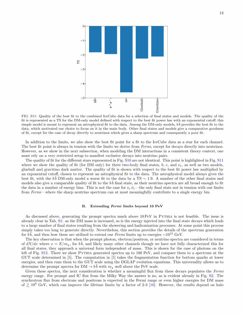
13

bb

e+

e

Glu

ebal

l

Gra

vitin

o5

4

3

2

1

0

TS

FIG. S11: Quality of the best fit to the combined IceCube data for a selection of final states and models. The quality of thefit is represented as a TS for the DM-only model defined with respect to the best fit power law with an exponential cutoff; thissimple model is meant to represent an astrophysical fit to the data. Among the DM-only models, b b provides the best fit to thedata, which motivated our choice to focus on it in the main body. Other final states and models give a comparative goodnessof fit, except for the case of decay directly to neutrinos which gives a sharp spectrum and consequently a poor fit.

In addition to the limits, we also show the best fit point for a fit to the IceCube data as a star for each channel.The best fit point is always in tension with the limits we derive from Fermi, except for decays directly into neutrinos.However, as we show in the next subsection, when modeling the DM interactions in a consistent theory context, onemust rely on a very restricted setup to manifest exclusive decays into neutrino pairs.

The quality of fit for the different stars represented in Fig. S10 are not identical. This point is highlighted in Fig. S11where we show the quality of fit (for DM only) for three two-body final states, b, e, and νe, as well as two models,glueball and gravitino dark matter. The quality of fit is shown with respect to the best fit power law multiplied byan exponential cutoff, chosen to represent an astrophysical fit to the data. The astrophysical model always gives thebest fit, with the b b DM-only model a worse fit to the data by a TS ∼ 1.9. A number of the other final states andmodels also give a comparable quality of fit to the b b final state, as their neutrino spectra are all broad enough to fitthe data in a number of energy bins. This is not the case for νe νe—the only final state not in tension with our limitsfrom Fermi—where the sharp neutrino spectrum can at most meaningfully contribute to a single energy bin.

B. Extending Fermi limits beyond 10 PeV

As discussed above, generating the prompt spectra much above 10 PeV in Pythia is not feasible. The issue isalready clear in Tab. S1: as the DM mass is increased, so is the energy injected into the final state decays which leadsto a large number of final states resulting from the showering and hadronization processes. At some point this processsimply takes too long to generate directly. Nevertheless, this section provides the details of the spectrum generationfor b b, and then how these are utilized to extend our Fermi limits up to energies ∼1012 GeV.

The key observation is that when the prompt photon, electron/positron, or neutrino spectra are considered in termsof dN/dx where x = E/mχ, for b b, and likely many other channels though we have not fully characterized this forall final states, they approach a universal form independent of mass. This is shown for the case of photons on theleft of Fig. S12. There we show Pythia generated spectra up to 100 PeV, and compare them to a spectrum at theGUT scale determined in [5]. The computation in [5] takes the fragmentation function for bottom quarks at lowerenergies, and then runs them to the GUT scale using the DGLAP evolution equations. This universality allows us todetermine the prompt spectra for DM→ b b with mχ well above the PeV scale.

Given these spectra, the next consideration is whether a meaningful flux from these decays populates the Fermienergy range. For prompt and IC flux from the Milky Way the answer is no, as is evident already in Fig. S2. Thesynchrotron flux from electrons and positrons is expected in the Fermi range or even higher energies for DM massof & 109 GeV, which can improve the lifetime limits by a factor of 2-3 [10]. However, the results depend on halo

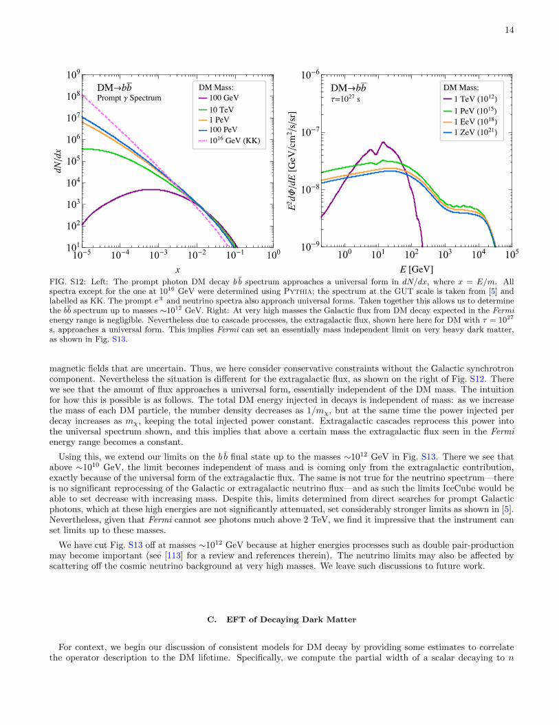
14

10-5 10-4 10-3 10-2 10-1 100101

102

103

104

105

106

107

108

109

/

→ γ

()

100 101 102 103 104 10510-9

10-8

10-7

10-6

[]

Φ/[

///]

→τ= ()

()

()

()

FIG. S12: Left: The prompt photon DM decay b b spectrum approaches a universal form in dN/dx, where x = E/m. Allspectra except for the one at 1016 GeV were determined using Pythia; the spectrum at the GUT scale is taken from [5] andlabelled as KK. The prompt e± and neutrino spectra also approach universal forms. Taken together this allows us to determinethe bb spectrum up to masses ∼1012 GeV. Right: At very high masses the Galactic flux from DM decay expected in the Fermienergy range is negligible. Nevertheless due to cascade processes, the extragalactic flux, shown here here for DM with τ = 1027

s, approaches a universal form. This implies Fermi can set an essentially mass independent limit on very heavy dark matter,as shown in Fig. S13.

magnetic fields that are uncertain. Thus, we here consider conservative constraints without the Galactic synchrotroncomponent. Nevertheless the situation is different for the extragalactic flux, as shown on the right of Fig. S12. Therewe see that the amount of flux approaches a universal form, essentially independent of the DM mass. The intuitionfor how this is possible is as follows. The total DM energy injected in decays is independent of mass: as we increasethe mass of each DM particle, the number density decreases as 1/mχ, but at the same time the power injected perdecay increases as mχ, keeping the total injected power constant. Extragalactic cascades reprocess this power intothe universal spectrum shown, and this implies that above a certain mass the extragalactic flux seen in the Fermienergy range becomes a constant.

Using this, we extend our limits on the b b final state up to the masses ∼1012 GeV in Fig. S13. There we see thatabove ∼1010 GeV, the limit becomes independent of mass and is coming only from the extragalactic contribution,exactly because of the universal form of the extragalactic flux. The same is not true for the neutrino spectrum—thereis no significant reprocessing of the Galactic or extragalactic neutrino flux—and as such the limits IceCube would beable to set decrease with increasing mass. Despite this, limits determined from direct searches for prompt Galacticphotons, which at these high energies are not significantly attenuated, set considerably stronger limits as shown in [5].Nevertheless, given that Fermi cannot see photons much above 2 TeV, we find it impressive that the instrument canset limits up to these masses.

We have cut Fig. S13 off at masses ∼1012 GeV because at higher energies processes such as double pair-productionmay become important (see [113] for a review and references therein). The neutrino limits may also be affected byscattering off the cosmic neutrino background at very high masses. We leave such discussions to future work.

C. EFT of Decaying Dark Matter

For context, we begin our discussion of consistent models for DM decay by providing some estimates to correlatethe operator description to the DM lifetime. Specifically, we compute the partial width of a scalar decaying to n

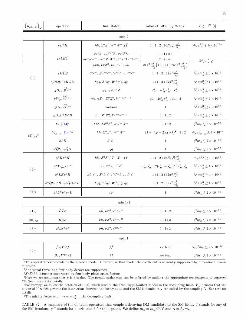
15

(RSU(2)

)Y

operator final states ratios of BR’s, mχ TeV τ & 1027 [s]

spin 0

(0)0

χH†H hh, Z0Z0,W+W−,ff 1 : 1 : 2 : 16Ncy2fv2

m2χ

mχ/Λ2 & 9× 1079a

χ (LH)2ννhh, ννZ0Z0, ννZ0h, 1 : 1 : 2 :

Λ4/m5χ & 1

νe−hW+, νe−Z0W+, e−e−W+W+, 2 : 2 : 4 :

ννh, ννZ0, νe−W+, νν 24π2 v2

m2χ

(1 : 1 : 1 : 768π2 v2

m2χ

)χHLE h`+`−, Z0`+`−, W±`∓ν, `+`− 1 : 1 : 2 : 32π2 v2

m2χ

Λ2/m3χ & 4× 1029

χHQU , φHQD hqq, Z0qq, W±q′q, qq 1 : 1 : 2 : 32π2 v2

m2χ

Λ2/m3χ & 1× 1030

χBµν(∼)

B µν γγ, γZ, ZZ c4W : 2c2W s2W : s4W Λ2/m3χ & 2× 1031

χWµν

(∼)

W µν γγ, γZ0, Z0Z0, W+W− b s4W : 2c2W s2W : c4W : 2 Λ2/m3χ & 6× 1031

χGµν(∼)

G µν hadrons 1 Λ2/m3χ & 2× 1032

χDµH†DµH hh, Z0Z0, W+W− c 1 : 1 : 2 Λ2/m3χ & 3× 1030

(2)1/2d

Vλ [114]e hhh, hZ0Z0, hW+W− 1 : 1 : 2 g2mχ . 2× 10−53

Vcβ−α [114]e,f hh, Z0Z0, W+W−(1 + (λT − 2λA)/λ

)2: 1 : 2 mχ/c2β−α & 4× 1048

φLE `+`− 1 g2mχ . 2× 10−56

φQU , φQD qq 1 g2mχ . 6× 10−57

(3)0

φaHσaH hh, Z0Z0,W+W−,ff 1 : 1 : 2 : 16Ncy2fv2

m2χ

mχ/Λ2 & 9× 1079

φaWaµνB

µν γγ, Z0γ, Z0Z0 c2W s2W : 2(c2W − s

2W

)2: c2W s2W Λ2/m3

χ & 1× 1031

φaLEσaH h`+`−, Z0`+`−, W±`∓ν, `+`− 1 : 1 : 2 : 32π2 v2

m2χ

Λ2/m3χ & 4× 1029

φaQUσaH, φaQDσaH hqq, Z0qq, W±q′q, qq 1 : 1 : 2 : 32π2 v2

m2χ

Λ2/m3χ & 1× 1030

(3)1 φaLT σaσ2L νν 1 g2mχ . 2× 10−56

spin 1/2

(1)0 HLψ νh, νZ0, `±W∓ 1 : 1 : 2 g2mχ . 2× 10−56

(2)1/2 HψE νh, νZ0, `±W∓ 1 : 1 : 2 g2mχ . 2× 10−56

(3)0 HLσaψa νh, νZ0, `±W∓ 1 : 1 : 2 g2mχ . 2× 10−56

spin 1

(0)0fγµV ′µf ff see text Ncg2mχ . 2× 10−56

BµνF ′µν/2 ff see text g2mχ . 4× 10−56

aThis operator corresponds to the glueball model. However, in that model the coefficient is naturally suppressed by dimensional trans-mutation.bAdditional three- and four-body decays are suppressed.cZ0Z0hh is further suppressed by four-body phase space factors.dHere we are assuming that χ is a scalar. The pseudo-scalar case can be inferred by making the appropriate replacements to conserve

CP. See the text for details.eFor brevity, we follow the notation of [114], which studies the Two-Higgs-Doublet model in the decoupling limit. VX denotes that the

potential V which governs the interactions between the heavy state and the SM is dominantly controlled by the coupling X. See text fordetailsfThe mixing factor cβ−α → v2/m2

χ in the decoupling limit.

TABLE S2: A summary of the different operators that couple a decaying DM candidate to the SM fields. f stands for any ofthe SM fermions, q(′) stands for quarks and ` for the leptons. We define mχ = mχ/PeV and Λ = Λ/mPl .

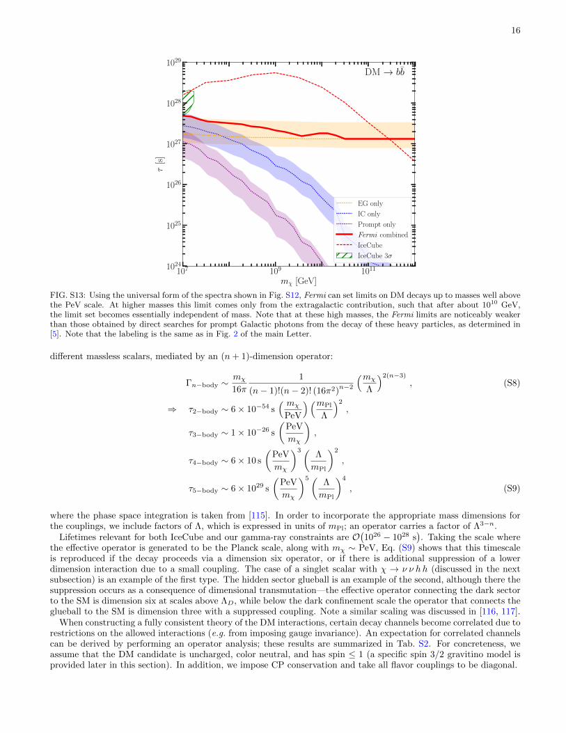
16

107 109 1011

mχ [GeV]

1024

1025

1026

1027

1028

1029

τ[s

]

DM → bb

EG only

IC only

Prompt only

Fermi combined

IceCube

IceCube 3σ

FIG. S13: Using the universal form of the spectra shown in Fig. S12, Fermi can set limits on DM decays up to masses well abovethe PeV scale. At higher masses this limit comes only from the extragalactic contribution, such that after about 1010 GeV,the limit set becomes essentially independent of mass. Note that at these high masses, the Fermi limits are noticeably weakerthan those obtained by direct searches for prompt Galactic photons from the decay of these heavy particles, as determined in[5]. Note that the labeling is the same as in Fig. 2 of the main Letter.

different massless scalars, mediated by an (n+ 1)-dimension operator:

Γn−body ∼mχ

16π

1

(n− 1)!(n− 2)! (16π2)n−2

(mχ

Λ

)2(n−3), (S8)

⇒ τ2−body ∼ 6× 10−54 s( mχ

PeV

)(mPl

Λ

)2,

τ3−body ∼ 1× 10−26 s

(PeV

mχ

),

τ4−body ∼ 6× 10 s

(PeV

mχ

)3(Λ

mPl

)2

,

τ5−body ∼ 6× 1029 s

(PeV

mχ

)5(Λ

mPl

)4

, (S9)

where the phase space integration is taken from [115]. In order to incorporate the appropriate mass dimensions forthe couplings, we include factors of Λ, which is expressed in units of mPl; an operator carries a factor of Λ3−n.

Lifetimes relevant for both IceCube and our gamma-ray constraints are O(1026 − 1028 s

). Taking the scale where

the effective operator is generated to be the Planck scale, along with mχ ∼ PeV, Eq. (S9) shows that this timescaleis reproduced if the decay proceeds via a dimension six operator, or if there is additional suppression of a lowerdimension interaction due to a small coupling. The case of a singlet scalar with χ → ν ν hh (discussed in the nextsubsection) is an example of the first type. The hidden sector glueball is an example of the second, although there thesuppression occurs as a consequence of dimensional transmutation—the effective operator connecting the dark sectorto the SM is dimension six at scales above ΛD, while below the dark confinement scale the operator that connects theglueball to the SM is dimension three with a suppressed coupling. Note a similar scaling was discussed in [116, 117].

When constructing a fully consistent theory of the DM interactions, certain decay channels become correlated due torestrictions on the allowed interactions (e.g. from imposing gauge invariance). An expectation for correlated channelscan be derived by performing an operator analysis; these results are summarized in Tab. S2. For concreteness, weassume that the DM candidate is uncharged, color neutral, and has spin ≤ 1 (a specific spin 3/2 gravitino model isprovided later in this section). In addition, we impose CP conservation and take all flavor couplings to be diagonal.

17

For a given model, we specify all possible renormalizable interactions with the SM fields. We present the lowestdimension operator (up to dimension six) which leads to a final state of interest, such that the branching ratio (BR)does not vanish asmχ →∞. We comment that in the survey below we have not performed a detailed phenomenologicalstudy, so some models could suffer additional particle physics constraints which are not incorporated here.

We use the following notation to specify the quantum numbers of a state:

X ∼(RSU(2)

)Y, (S10)

where RSU(2) gives the representation under SU(2)W and Y is the hypercharge. Then the SM Higgs is denoted as

H ∼ (2)1/2 , (S11)

with a vacuum expectation value (VEV) v = 246 GeV. The SM lepton fields are given by

L ∼ (2)−1/2 , E ∼ (1)−1 , (S12)

and the quark fields are specified by

Q ∼ (2)1/6 , U ∼ (1)2/3 , D ∼ (1)−1/3 . (S13)

The SU(3)C representation is implicit, and SU(2)W -doublets (singlets) are left (right)-handed fields. In all cases,flavor indices are suppressed. The field-strength tensors for hypercharge, weak, and strong forces are denoted as Bµν ,

Wµν and Gµν , respectively, and their duals are denoted with a tilde. In addition, we use H = i σ2H∗. The different

DM candidates are characterized by their electroweak quantum numbers using the same notation. In cases where anadditional mass scale is needed (such as a cut-off), it is denoted as Λ, and we use g for dimensionless extra parameters.In some of the cases the DM candidate is part of larger electroweak multiplet. Therefore, we denoted the full multipletusing φ, ψ or V (depending on the spin), and reserve χ for the DM candidate itself.

With the above notation in mind, an extensive EFT classification of decaying DM models is given in Tab. S2. Wehave organized this table by the spin of the DM, beginning with spin 0, and then further sub-divided into

(RSU(2)

)Y

representations. For each operator, we show the SM final states resulting from the DM decay. We then give thebranching ratios to these states in the limit where the DM mass is much larger than the TeV scale. Further weprovide the requirements on mχ ≡ mχ/PeV and Λ = Λ/mPl in order to have τ & 1027 s. When the operators aredimension 4, we instead give the requirement in terms of mχ and the dimensionless coupling g.

One example that demonstrates why it is important to frame constraints in terms of decay operators derives frommodel building for the νν final state relevant for IceCube. We will argue that it is not possible to write down aPeV mass DM state and corresponding decay operator for which the branching ratio is dominated by the νν channel,without introducing states with non-trivial quantum numbers (which implies additional new states at similar masses).

First, consider singlet scalar DM χ. In general, χ can be coupled to SM gauge neutral operators OSM through theoperator χ×OSM.4 The different possible operators are summarized in the upper part of Tab. S2. For a single DMstate χ, the only operator giving the ν ν final state is the dimension six operator

L ⊃ 1

Λ2χ(LH

)2, (S14)

which we will take to be restricted to the first generation for simplicity.5 As shown in Tab. S2, at ∼PeV masses, thefinal state ν ν hh, along with the other channels required to satisfy the Goldstone equivalence theorem, dominate,even though this is a four body decay. This behavior can be understood by realizing that at these masses it is moreappropriate to consider the electroweak symmetry preserving limit of the theory, where this is the only allowed decaymode. We will return to this operator in the next subsection, where we show that due to the additional final states is isstrongly constrained by Fermi (see Fig. S14). Finally, we include all other options for singlet scalar decay following ourguidelines specified above. Note that the operators χψ†Dµσ

µψ and χH†DµDµH can be mapped onto the operators

in Tab. S2 using the equations of motion.Next, we investigate the case that the DM candidate is the neutral component of a non-trivial SU(2)W multiplet, for

example a doublet or a triplet. Staring with the doublet case, note that mχ mh is the decoupling limit of two Higgs

4 If χ is charged under a beyond-the-SM symmetry, it can couple as(χ†χ

)× OSM. Then the DM will only decay if χ acquires a VEV.

This leads to similar phenomenology as in the uncharged case (up to a factor of the χ VEV divided by the new physics scale).5 Note that we are assuming dimension five operators of the form χ × LSM are suppressed by a symmetry, e.g. lepton number. This

requires that the physics at the Planck scale does not badly break this symmetry.

18

doublet model, which has been studied extensively—here we follow the conventions and notation of [114]. The threeheavy Higgs states, the scalar, pseudo-scalar and charged Higgs, all have similar masses up to electroweak breakingeffects set by the scale v. There are two valid DM candidates, the scalar and the pseudo-scalar. The spectrum anddominant decay modes depend on the details of the scalar potential as well as the choice of Yukawa couplings betweenthe SM fermions and the two Higgs doublets. For concreteness, we specify three representative scenarios for modelswhere the scalar is the DM: (i) Vλ: Three-body decays χ → hhh, hZ0 Z0, hW+W−; (ii) Vcβ−α : Two-body decays

χ → W+W−/Z0 Z0; (iii) Yukawa: Two-body decays χ → f f . The notation VX is shorthand for the regions of theparameter space where the X coupling dominates the decay phenomenology, following the notation of [114]. This issummarized in Tab. S2. If the DM is the pseudo-scalar instead, then similar modes are allowed with the appropriatereplacements to conserve CP, e.g. χ → Z0 hh. Finally, we emphasize that it is not possible to get direct decays toneutrinos for this model.

Next, we discuss the case where the DM is the neutral component of an SU(2)W triplet φa with hypercharge Y = 1;for simplicity we assume it does not obtain a VEV. Given our focus on neutrino final states, the following allowedinteraction is particularly interesting

L ⊃ g φaLTσaσ2L , (S15)

where g is a new Yukawa coupling and σa are the Pauli matrices acting on the SU(2)W indices. This operator impliesthat φa has lepton number two, and yields a 100% branching fraction for χ → ν ν. Since this operators requires theintroduction of a full triplet multiplet to preserve gauge invariance, there must also be a charged and doubled chargedscalar, with the same mass up to electroweak breaking corrections. The possible interaction and decay channels aregiven in Tab. S2.

We conclude our discussion of scalar DM candidates with one more example. If the neutrinos are Dirac fermions,then the low energy effective theory must include right handed neutrino states νR, and one could decay a singletscalar via the operator L ⊃ χνTR νR [118]. Due to neutrino oscillations, these right handed neutrinos will yield aline signature in active neutrinos. This example is different from χ → ν ν directly because there are no electroweakcorrections to the prompt decay into right handed (sterile) neutrinos, which implies that Fermi does not set a relevantconstraint.

We also consider the case where the DM particle has spin. Fermionic DM can be coupled to the SM via a Yukawa-like interaction. We consider the choices where the DM candidate is an SU(2)W singlet, doublet, or triplet, with theappropriate hypercharges chosen so that one of the states in the multiplet is a singlet (see Tab. S2). In case of massivespin-1 Z ′ DM, we assume that it is a singlet under the SM gauge group and acquires all (or most) of its mass froma new scalar VEV. We consider two possibilities in Tab. S2, (i) one or more of the SM fermions is charged under anadditional broken U(1) gauge symmetry; and (ii) kinetic mixing with the hypercharge gauge boson, see e.g. [119, 120]for some studies of this DM candidate. It is also possible that this particle is the manifestation of a broken gaugingof some subset of the SM global symmetries, e.g. the U(1) of B −L. In such a scenario, the resulting gauge couplingmust be extremely small to realize τ in the range of interest. Finally, for spin-3/2 DM, we will consider a specificR-parity violating model as discussed in the next sub-section.

D. Additional Models

In this section, we give limits on two additional DM models of interest beyond the example of a hidden sectorglueball decaying via the operator λD GDµν G

µνD |H|2/Λ2 discussed in the main Letter.

Gravitino DM whose decay is due to the presence of bi-linear R-parity violation (via the super-potential couplingW ⊃ Hu L) is a well studied scenario. If the gravitino, denoted by ψ3/2, is very heavy, it will decay via the following

four channels: ψ3/2 → ν γ, ν Z0, ν h, `±W∓ [121, 122]. For m3/2 near the weak scale, the branching ratios aresomewhat sensitive to the details of the SUSY breaking masses. However, once m3/2 v, the decay pattern quickly

asymptotes to 1 : 1 : 2 for the ν Z0, ν h, `±W∓ channels respectively, as expected from the Goldstone equivalencetheorem.

In Fig. S14 we show the constraints on decaying gravitino DM assuming the above decay modes, with branchingratios given as functions of mass in the inset, using the benchmark parameters of [121]. At masses below theelectroweak scale, the γν final state dominates. This channel is best searched for using a gamma-ray line search,which is beyond the scope of this work. For this reason, we only show our constraints for masses above mW . Notethat the region where decaying DM could provide a ∼3σ improvement over the null hypothesis for the IceCube, theultra-high-energy neutrino flux (green hashed region) is almost completely excluded by our gamma-ray constraints.The IceCube constraints, determined using the same methods discussed in the main body of this work, begin todominate at scales above ∼100 TeV.

19

In Fig. S14, we also show limits obtained on the lifetime of the DM χ under the assumption that χ interacts withthe SM through the operator in Eq. (S14)—this model was discussed in detail in the previous subsection, see Tab. S2.The inset plot shows the branching ratios as a function of energy, and illustrates the transition from two- to three-to four-body decays dominating as the mass is increased. In this case as well, almost the entire range of parameterspace relevant for IceCube is disfavored by our gamma-ray limits.

We use FeynRules 2.0 [123] to generate the UFO model files, which are then fed to Mad-Graph5 aMC@NLO [124, 125] to compute the parton-level decay interfaced with Pythia for the shower-ing/hadronization of the decays χ → ν ν hh , ν ν Z0 h , ν ν Z0 Z0 , ν e− hW+ , ν e− Z0W+ , e− e−W+W+ andχ→ ν ν h , ν ν Z0 , ν e−W+.

102 104 106

mχ [GeV]

1024

1025

1026

1027

1028

1029

τ[s

]

Gravitino DM

EG only

IC only

Prompt only

Fermi combined

IceCube

IceCube 3σ

102 104 106

mχ [GeV]

0.0

0.5

1.0

Bra

nch

ing

rati

os

W`

Zν

hν

102 104 106

mχ [GeV]

1024

1025

1026

1027

1028

1029

τ[s

]

χ(LH)2/Λ2

EG only

IC only

Prompt only

Fermi combined

IceCube

IceCube 3σ

102 104 106

mχ [GeV]

0.0

0.5

1.0

Bra

nch

ing

rati

os

2-body

3-body

4-body

FIG. S14: Constraints on decaying gravitino DM (left) and DM decaying via the operator χ (LH)2 (right). Notation andlabeling is as in Fig. 2 in the main Letter.