games with dynamic externalities and climate change experiments …€¦ · games with dynamic...

Games with Dynamic Externalities and Climate ChangeExperiments

By Tatsuyoshi Saijo ∗, Katerina Sherstyuk†, Nori Tarui‡,and Majah-Leah Ravago§

May 2009COMMENTS WELCOME

AbstractWe report on laboratory experiments with series of games with dynamic externali-

ties, where the current actions of each player affect not only the player’s payoff today,but also the group payoffs levels of the game that will be played tomorrow. The mo-tivating example is the climate change problem, where welfare opportunities (payofflevels) in the present depend on the stock of greenhouse gases (GHG) accumulated inthe past, with higher current emissions leading to lower future payoffs. We investigatewhether socially optimal actions may be sustained in such dynamic externality gameswith changing payoffs if no explicit enforcement mechanisms are present. Two mainexperimental treatments are studied. In the Long-Lived treatment, the dynamic gameis played by the same group of subjects who interact for many periods (generations).This represents an idealistic setting where countries’ decision-makers and citizens aremotivated by long-term welfare of their countries. In the Inter-Generational treat-ment, the dynamic game is played by several groups (generations) of subjects, withlater generations having access to history and advice from previous generations. Thisrepresents a more realistic setting in which the countries’ decision-makers and citizensmay be motivated more by the immediate welfare and may care only partially aboutthe future generations’ payoffs. Experimental results indicate that in the Long-Livedtreatment, many groups of subjects were able to avoid the myopic Nash outcome and tosustain or come back close to the socially optimal emissions and GHG stock levels. Inthe Inter-Generational treatments, subject decisions were often myopic. These findingssuggest that international dynamic enforcement mechanisms (treaties) are necessaryto control GHG emissions.

Key words: economic experiments; dynamic externalities; inter-generational games;climate change

∗Osaka University. Email: [email protected]†Corresponding author. Department of Economics, University of Hawaii at Manoa, 2424 Maile Way,

Honolulu, HI 96822. Email: [email protected]‡University of Hawaii at Manoa. Email: [email protected]§University of Hawaii at Manoa. Email: [email protected]

1

1 Introduction

Many economic problems involve dynamic externalities, where agents’ decisions in the cur-rent period influence the welfare of the agents in the future periods. Global environmentalissues such as climate change, management of international water resources, and loss ofbiodiversity provide examples. The actions by the current decision makers influence thewelfare of the future generations due to changes in state variables such as the atmosphericconcentration of greenhouse gases, water availability, or species richness.

Efficient resource allocations with global dynamic externalities require cooperation bysovereign countries over a long time horizon, possibly involving multiple generations of de-cision makers. There is an increased interest among researchers as well as policymakersover institutional arrangements that enhance cooperation in such contexts. A large scientificliterature warns of the dangers of failing to successfully address these issues and continuingbusiness-as-usual. As for climate change, the Intergovernmental Panel on Climate Changeconcluded that continued emissions of greenhouse gases (GHG) would likely lead to signif-icant warming over the coming centuries with the potential for large consequences on theglobal economy (IPCC 2007).

While natural and environmental scientists may inform the policy-makers about thephysical consequence of GHG emission reductions, implementation of mitigation efforts byspecific countries remains a global economic problem. Global dynamic externalities areespecially challenging because they have the features of the global public goods, where eachcountry’s mitigation efforts benefit all countries but impose private costs, giving rise to thefree-rider problem among countries; and long term aspects, where the effect of current actionscan be felt into the distant future ( Nordhaus 1994, Schlenker and Roberts 2006, Schlenkeret al. 2006, IPCC 2007 Chapter 10, Dutta and Radner, forthcoming). The countries’governments may be short-sighted and motivated by their countries’ immediate welfare,rather than the long-term effect of emissions on future generations.

Though many studies analyze international treaties for climate change mitigation, re-search that takes into account the above features is only starting to emerge. In practice,countries have adopted a number of international environmental agreements that differ intheir performances and specifications of mechanisms to support cooperation. Some agree-ments adopt a voluntary, non-legally binding framework (e.g. the Asia-Pacific Partnershipon Clean Development and Climate that promotes cooperation over technology developmentto reduce greenhouse gas emissions) while others specify binding targets (e.g. the MontrealProtocol on Substances That Deplete the Ozone Layer, the Kyoto Protocol to the United Na-tions Framework Convention on Climate Change). It is still an open question whether strict

2

enforcement mechanisms are necessary to support long-term cooperation among countries,or whether a voluntary cooperation may sustain dynamically socially optimal outcomes.

This paper uses the experimental economics methodology to investigate whether sociallyoptimal actions may be sustained in dynamic externality games with changing payoffs ifno explicit enforcement mechanisms (treaties) are present. We first model infinitely liveddecision makers (representing an idealistic setting where the countries’ governments are mo-tivated by long-term welfare for their countries), and then extend the analysis to an inter-generational decision making framework (representing a more realistic setting in which thecountries’ governments may be motivated more by their countries’ immediate welfare). Thestudy considers the role of intergenerational caring, access to history and information aboutfuture consequences of current actions, and social learning in establishing and sustainingcooperation.

Experimental research has proven extremely useful in evaluating alternative policy in-struments, particularly those that are prohibitively costly to test in the field (Eckel andLutz, 2003). The use of university students as subjects allows to evaluate, on a small scale,performances of different treaties, before such treaties may be tested with policy-makers,either in the laboratory or in the field (e.g., Bohm, 1999). A growing experimental literatureindicates that appropriately designed and tested economic mechanism may help to alleviateenvironmental problems and provide useful advice to policy-makers (Bohm, 2003; Cason andGangadharan, 2006). However, most experimental studies on climate change mitigation fo-cus on relatively short-term (Bohm, 1999; Cason, 2003) or national (Holt et al, 2007) aspectsof the problem, while the current research focuses on the global (international) and dynamiclong-term aspects.

The paper builds on several existing streams of experimental literature, as we discussnext.

In its dynamic feature, the climate change problem is similar to dynamic common poolresource (CPR) games. Herr et al. (1997) study static and dynamic externalities in the com-mons using finite-period CPR games. They report that subject behavior was generally awayfrom the social optimum and more consistent with non-cooperative solution benchmarks.Chermak and Krause (2002) study the dynamic CPR problem in an overlapping generationssetting. The dynamic externality was present in that today’s resource use determined thefuture resource constraint. The authors report that subject behavior was heterogeneous;yet, in 16% of cases, groups depleted the resource prior to the terminal period. Fischer etal. (2004) investigate altruistic restraint in CPR exploitation when subjects are explicitlyinformed that their resource use affects the resource level that will be available to the sub-jects in the next generation. The subjects were given no monetary incentives to care about

3

future generations. They find no effect of intergenerational concerns on subject behavior,but the subjects expected others to care about the future generations and to cut down theirresource use, the behavior that the authors call “optimistic free-riding:” “I free-ride, but Iexpect others not to”.

Several experimental studies explore intergenerational games in contexts other than CPR.Using a finite-horizon pension game experiment, van der Heijden et al. (1998) found a sub-stantial degree of voluntary transfers across generations of players. On the other hand,Offerman et al. (2001) report that subjects in their overlapping generations game seldomsupported cooperative actions even when they were recommended to play grim-trigger strate-gies.

The intergenerational aspect of the climate change problem suggests that findings onintergenerational learning and advice (Schotter and Sopher, 2003; Ballinger et al. 2003;Chaudhuri et al, 2009) are relevant. For a setting with chains of groups of subjects playingrecurring voluntary contributions public good games, Chaudhuri et al. (2006) report thatcommon knowledge of advice had a positive and significant effect on contributions. Forthe climate change mitigation problem, social learning may play a significant role, sincehistories of past actions, opinions and recommendations of scientists and politicians couldbe made available to the public and to the future generations. We give the subjects in ourexperiment access to history and advice from previous generations to enhance the possibilityof sustaining dynamically optimal outcomes.

In this paper we describe an experiment that was designed and conducted to investigatehow games with dynamic externalities, such as climate change, may evolve without explicittreaties among players. The rest of the paper is organized as follows. Section 2 overviewsthe underlying theoretical model of games with dynamic externalities and defines theoreticalbenchmarks that would be further used to evaluate experimental results. Section 3 discussesexperimental design, and Section 4 presents the results. Section 5 discusses conclusions andopen questions.

2 Theoretical model

The underlying model of the dynamic externality game among countries is very similarto the one developed by Dutta and Radner for infinitely live palyers (2004, 2005, 2006,forthcoming). We now review the model and benchmark solutions with infinite horizongovernments, as discussed by Dutta and Radner. We then discuss how the setting maybe extended to multiple, finitely lived generations of governments in each country using analternative generational game framework.

4

2.1 Games with infinitely-lived players

Model environment: The set of players consists of N ≥ 2 countries. In each periodt = 1, 2, . . ., country i chooses an emission xit ∈ [0, xi > 0], where xi is the maximum feasibleemission level. The pollution stock S evolves across periods according to the followingequation:

St+1 = λSt + Xt, t = 0, 1, . . . , (1)

where λ ∈ [0, 1] represents the retention rate of the pollution stock; hence 1 − λ representsthe natural rate of decay of pollution (0 ≤ λ < 1), and Xt ≡ ∑

i xit. The initial stock S0 isgiven.

The period-wise return of player i, πi, in period t consists of two components: the (net)benefit from its own emission and the damages due to the existing pollution stock in periodt:

πi(xit, St) = Bi(xit) − Di(St), (2)

where Bi is strictly concave, differentiable, and has a unique finite maximum xi that liesbetween 0 and xi. For simplicity, we adopt a simple and common to all players quadraticbenefit function B(x) = ax − 1

2cx2, which implies a unique finite maximum x = a/c. The

damage function satisfies D′i > 0, D′′

i ≥ 0. Following Dutta and Radner, we assume a linear(and common among players) damage function D(St) = dSt. The parameter d > 0 representsthe marginal damages due to the stock of pollution.

Given a discount factor δ ∈ (0, 1), country i’s payoff is given by the present value of theperiod-wise returns

∑∞t=0 δtπi(xit, St). Countries have complete information and there is no

uncertainty in the model. In each period, each country observes the history of pollutionstock transition and all countries’ previous emissions.

Benchmark solutions Consider the following four benchmark emissions allocations.First Best solution (FB): Assume that all countries’ return functions are measured

in terms of a common metric. Then the First Best, or the cooperative emission allocationmaximizes the sum of N countries’ payoffs and hence solves the following problem:

max∞∑

t=0

N∑

i=1

δtπi(xit, St) subject to the constraints (1). (3)

The solution to this problem generates a sequence of emissions {x∗t }∞

t=0 where x∗t = {x∗

it}Ni=1.

With the linear damage function, the solution is constant over periods, is independent ofstock level and satisfies: B′(x∗

it) = δNd1−δλ

, for all i, t.Sustainable solution (Sus): This is a special case of the first best solution when

δ = 1, i.e. the social discount factor is set equal to one. Sus corresponds to the optimal GHG

5

emission control supported by the Stern Review (2006) and several other economic studies,which adopt very low social discount rates in their analysis.

Myopic Nash solution (MN): With δ = 0, the Nash equilibrium emission of playeri, xi, solves B′

i(xi) = 0. Because there is no static externality, this emission level is optimalfor generation t as a whole as well. We call {xi} the Myopic Nash (MN) solution.1 Thequadratic benefit function B(x) = ax − 1

2cx2 implies a unique MN solution x = a/c.

Markov Perfect equilibrium (MP): The above dynamic game has many subgameperfect equilibria. We take the outcome of a Markov perfect equilibrium (MPE), whereeach country conditions its emission in each period on the current pollution stock, as anatural benchmark of the noncooperative outcome. In particular, an MPE of a simple formexists under some further assumptions on the period-wise return functions. For the abovemodel specification, the unique Markov perfect equilibrium where each country’s emission isindependent of the pollution stock level is given by x such that b′(x) = δd

1−λδ.

2.2 Games with multiple generations of players

To extend the above framework to a game with multiple generations of players (countries),we assume that each period in the model described above represents a distinct generation ofplayers. Hence, there are infinite number of generations of players, starting with generation0. Each generation consists of N players, and plays for one period. Let (i, t) represent the ithplayer in generation t. With this alternative setup, we call πi in equation (2) the concurrentpayoff of player (i, t). Assume the (total) payoff of player (i, t), Πit, is a δ-weighted sum ofthe concurrent payoff and player (i, t + 1)’s payoff:

Πit = πit + δΠit+1. (4)

This specification allows for inter-generational caring, where 0 ≤ δ ≤ 1 is interpreted as theweight that player i in generation t puts on the on the next generation’s total payoff relativeto own concurrent payoff. As in section 2.1, we can then define four benchmark solutions.The First Best solution (FB) given the intergenrational welfare weights δ solves theproblem (3), and hence is the same as the first best allocation in the original model. For thespecial cases where δ = 1 and δ = 0, we have the Sustainable solution (Sus) and theMyopic Nash solution (MN) as defined in the previous subsection. A simple MarkovPerfect equilibrium (MP) is also defined analogously.

1Dutta and Randner refer to xi as the “business-as-usual” emission level of country i.

6

3 Experimental design

Overall design The experiment is designed to study subject behavior in dynamic exter-nality games modeled as in section 2. Groups consisting of N = 3 subjects each participatedin chains of linked decision series (generations). In each decision series, each subject in agroup chose between 1 and 11 tokens (representing a level of emissions by his country), giveninformation about the current payoffs from own token choices, and the effect of group tokenchoices on future series’ (generations’) payoffs.2 The payoffs were given in a tabular form,as illustrated in Figure 1.

FIGURE 1 AROUND HERE

From the figure, a subject’s current payoff is not affected by current choices of othersin the group (no static externality) and is maximized at xi = 7 (Myopic Nash solution);however, the total number of tokens invested by the group in the current series affects thepayoff level in the next series. The payoff level represents the current welfare opportunities;it decreases as the underlying GHG emissions stock increases. The payoff scenario in thefigure illustrates how the payoffs would evolve across series if the total number of tokensordered by the group stays at 21 in each series (corresponding to MN outcome).

The parameter values are chosen so that all four theoretical benchmarks ( Sustainable:xi = 3; First Best: xi = 4; Markov Perfect: xi = 6; and Myopic Nash: xi = 7) for individualtoken investments (emission levels) are distinct from each other and integer-valued. Thecooperative FB outcome path gives the subjects substantially higher expected stream ofpayoffs than the MN or the MP outcome.

To study whether sustaining cooperation without explicit treaties is at all possible undersome conditions, we chose parameter values favorable for cooperation (rather than realistic):Payoff functions were identical across subjects; the starting stock S0 was set at the FirstBest steady state level; and the GHG stock retention rate was low, λ = 0.3, which allowedfor fast recovery from high stock levels.

The experiment continued for several series (generations). To model an infinitely repeatedgame and eliminate end-game effects, a random termination rule was used. A randomizationdevice (a bingo cage) was applied after each series (generation) to determine whether the

2In fact, each series consisted of three decision rounds, where subjects made token choices. One of therounds was then chosen randomly as a paid round, and was also used to determine next series’ payoff level.We decided to have more than one round in a series to give the subjects an opportunity to learn betterthe behavior of other subjects in their group, and also to allow subjects in inter-generational treatments (tobe discussed below) make more than one decision. Subject decisions were rather consistent across roundswithin series. In what follows, we will therefore focus on the data analysis for the chosen (paid) rounds ofeach series; see Section 4 below.

7

experiment continues to the next series. The continuation probability induces the corre-sponding discount factor in the experimental setting; the random termination is importantto closely follow the theoretical model (Dal Bo, 2005). To obtain reasonably (but not ex-cessively) long chains of series (generations), the continuation probability of 3/4 was usedbetween series. This induced the corresponding discount factor δ = 0.75.

Treatments To study how games with dynamic externalities evolve with infinitely-livedplayers as compared to generations of short-lived players, the experimental design includesthe following treatments:

(1) Baseline Long-Lived (LL): The same group of subjects makes decisions forall generations; each subject’s payoff is her cumulative payoff across all generations. Thistreatment corresponds to the model as discussed in section 2.1, and represents an idealisticsetting where decision makers are motivated by long-term welfare for their countries. Thetreatment investigates whether social optimum may be sustained in dynamic externalitygames played by infinitely lived players.

(2) Intergenerational Selfish (IS) : A separate group of subjects makes decisionsfor each generation; each subjects’ total payoff is equal to her concurrent payoff, i.e., it isbased on her performance in her own generation only. Theoretically, this payoff structureinduces no weight to be put on the next generations’ welfare, thus suggesting Myopic Nashbehavior if subjects are motivated solely by own monetary payoffs. This treatment representsa possibly more realistic setting in which the countries’ decision makers are motivated mostlyby their countries’ immediate welfare. The treatment studies whether subjects may exhibitinter-generational caring when they are made aware of the dynamic effect of their decisionson the follower’s payoffs.

(3) Intergenerational Long-sighted (IL): A separate group of subjects makesdecisions for each generation; each subjects’ payoff is equal to her concurrent payoff (i.e.,her payoff in her own generation), plus the sum of all her followers’ concurrent payoffs.3

The cumulative payment in IL keeps the setup consistent with the theory in Section 2.2.This suggests that the behavior in this treatment should theoretically be no different than inthe baseline LL treatment. This treatment studies whether subjects restrain their emissionsin the inter-generational setting when they are made aware of the dynamic effect of their

3Unlike experimental studies on intergenerational advice in recurring games without random termination,such as Chaudhuri et al. (2006), our experimental design does not allow to put only partial weight onfuture generations payoff, as it would induce double discounting across generations: through continuationprobability and through partial weight put on future payoffs. An alternative of paying for one of thegenerations randomly can also be shown to create the present generation bias, as we show in a companionpaper; see Saijo et al. (2009). Making a subjects’ payoff depend on own concurrent payoff and on theimmediate follower’s concurrent payoff only creates incentives for myopic advice.

8

decisions on the follower’s payoffs and are fully motivated by monetary incentives to careabout the future.

In all treatments, the experimental design included elements that may help cooperationin the context of climate change mitigation. First, subjects’ expectations about the others’choices were solicited, to study whether subjects’ willingness to cut down own emissions(tokens) is correlated with their expectations of similar actions by others.

Further, to study social learning, at the end of each series each subject was asked tosend “advice” to the next series (generations) in the form of suggested token levels, and anyverbal comment. This advice, along with the history of token orders, was then displayed toall subjects in his group in all the the following series (generations). For the climate changemitigation problem, knowledge of history and social learning may play a significant role,since histories of past actions, opinions and recommendations of scientists and politicianscould be made available to the public and to the future generations.

Procedures The experiments were computerized using z-tree software (Fischbacher, 2007).Several (up to three) independent groups of subjects, with three subjects in each group, par-ticipated in each experimental session. In the baseline LL sessions, the same groups ofsubjects made token decisions in all decision series carried out within the same session ,until the experiment stopped. In the inter-generational IS and IL sessions, each group ofsubjects participated in one decision series only, after which the randomization device de-termined if the experiment would continue to the next series which would take place in thenext session with new participants. Decision series of the same group in LL treatment (or achain of groups in IS and IL treatments) were inter-linked through the dynamic externalityfeature of payoffs, as explained above, and through history and advice from previous seriesthat was passed on to the next series in a chain.

In all treatments and sessions, the subjects went through extensive training before par-ticipating in paid series. The training included: (a) Detailed instruction period (see Ex-perimental Instructions, given in Appendix A), which included examples of dynamic payoffscenarios as illustrated in Figure 1 (see Examples of Payoff Scenarios, Appendix B); followedby (b) Practice, consisting of five to seven linked series, for which the subjects were paid aflat fee of $10. Extensive practice was necessary to allow the subjects an opportunity to learnthrough experience the effect of dynamic externalities on future payoffs.4 In addition, duringeach decision round the subjects had access to a payoff calculator which allowed them toevaluate payoff opportunities for several series (generations) ahead given own token choices

4We felt that extensive training was especially important to ensure that the subjects fully understood thedynamic externality aspect of the game in the inter-generational treatments, where each subject participatedin only one paid decision series.

9

and choices of the others in the group.Each experimental session lasted up to three hours in the LL treatment, and up to two

hours in the IS and IL treatment, including 60-75 minutes of instructions and training. Theexchange rates were set at $ 100 experimental = $ 1 US in the LL and IL treatments, and$ 100 experimental = $ 4 US in the IS treatment (note that the expected length of a chain,given the continuation probability of 3/4, is 4 series; hence the exchange rates were adjustedacross the treatments accordingly). The expected payment per subject was set at around$35 per subject, including $10 flat training fee.

4 Results

Four to five independent chains of groups of subjects were conducted under each of the base-line LL, intergenerational IS and intergenerational IL treatments at the University of Hawaiiat Manoa. Subjects were recruited from undergraduate students in the college of social sci-ences. Each chain lasted between 3 and 9 series (generations). Table 1 lists the durationof each chain, along with average group tokens and average recommended group tokens bytreatment. Figures 2-3 illustrate the evolution of group tokens and the corresponding stocklevels for each chain, grouped by treatment.

TABLE 1 and FIGURES 2-3 AROUND HERE

Figures 2 and 3 suggest very different dynamics of group tokens (and, correspondingly,of the stock) across treatments. Figure 2 indicates that, in the LL treatment, all groups ofsubjects were able to avoid the Myopic Nash outcome and to sustain or come back close tothe First Best group tokens and stock levels. In comparison, group tokens in the IS and ILtreatments were considerably higher. The mean group token order in the LL was 13.34 andnot significantly different from the FB level of 12. This compares to the mean group tokenorder of 18.00 in IS, which is still below the Myopic Nash level of 21. The mean group tokenorder in the IL treatment was significantly more variable across chains, with a mean of 15.28,which is almost exactly half-way between the FB level of 12 and MP level of 18. Casualcomparison of the stock dynamics across treatments again suggests that the groups in theLL treatment were moving towards the FB stock levels, whereas the stock was increasingrapidly in the IS treatment, and exhibited large variance within the IL treatment.

While comparison of chain averages, as given in Table 1, is suggestive of differences acrosstreatments, it may be misleading since it does not capture the dynamics of group tokens andstock within chains. An analysis of evolution of variables of interest in time is necessaryto capture the adjustment dynamics across series, and to evaluate and compare long-term

10

convergence levels for group tokens and stocks across treatments. The following model,adopted from Noussair et al (1997), is used to analyze the effect of time on the outcomevariable (group tokens or stock) within each treatment:

yit =N∑

i=1

B0iDi(1/t) + (BLLDLL + BISDIS + BILDIL)(t − 1)/t + uit, (5)

where i = 1, .., N , is the chain index, N = 13 is the number of independent chains in allthree treatments, and t is the series index. Di is the dummy variable for chain i, whileDLL, DIS and DIL are the dummy variables for the corresponding treatments LL, IS and IL.Coefficients B0i estimate chain-specific starting levels for the variable of interest,5 whereasBLL, BIS and BIL are the treatment-specific asymptotes for the dependent variable. Thus,we allow a different origin of convergence process for each chain, but estimate common, withintreatments, asymptotes. The error term uit is assumed to be distributed normally with meanzero. We performed panel regressions using feasible generalized least squares estimation,allowing for first-order autocorrelation within panels and heteroscedastisity across panels.

The results of regression estimations of group tokens and stock convergence levels aregiven in Tables 2 and 3. Along with listing the estimated asymptotes for each treatment,the tables also display p-values for the test of their equivalence to the four theoretical bench-marks: Sus, FB, MP and MN.

The regression results are very clear. While the group tokens in the LL treatment convergeto 11.52, which is not significantly different from the FB level of 12 (p-value is 0.3941), thegroup tokens in the IS treatment converge to 18.14, which is not significantly different fromthe MP level of 18 (p-value is 0.7953), but is nevertheless below the MN level of 21. Thegroup tokens in the IL treatment converge to 15.94, which is above the FB level of 12 butbelow the MP of 18. The stocks converge to the FB level in the LL treatment (p-value is0.327), just under the MN level in the IS treatment, and the MP level in the IL treatment(p-value is 0.837). We conclude the following.

Conclusion 1 In the Long-Lived treatment, groups of subjects were able to avoid myopicdecisions, with group tokens and stock levels converging to the First Best levels. In contrast,in the Intergenerational Selfish treatment, group tokens and stock levels were converging tolevels just under the Myopic Nash benchmarks. Chains in the Intergenerational Long-sightedtreatment exhibited dynamics in between the FB and the MP predictions.

5Chain-specific starting coefficients B0i were estimated for group tokens and recommended group tokens.For the stock variable, we estimated a common starting level B0, as the starting stock was set at the FirstBest level for all chains.

11

We next consider the evolution of group advice across treatments. Table 1 suggeststhat while the average group number of recommended tokens in each treatment was slightlybelow the actual group tokens, the ranking of recommended tokens across treatments wasthe same as the ranking of actual group tokens. The average number of recommendedtokens for a group was 12.58 in the LL treatment, as compared to 16.62 in the IS treatment,as compared to 13.63 in the IL treatment. Evolution of recommended group tokens bytreatment, illustrated in Figure 4, suggests that recommended tokens in each treatment andchain followed a trend similar to that of actual tokens.

FIGURE 4 and TABLE 4 AROUND HERE

Regression analysis of recommended group tokens presented in Table 4 confirms that actualgroup tokens and recommended tokens were converging to the same theoretical benchmarks.In particular, the recommended tokens asymptote in the LL treatment was 11.48, which is notdifferent from the FB level of 12 (p-value is 0.1161). The recommended tokens asymptotein the IS treatment was 17.21, which is much higher than in the LL treatment, but isnevertheless below the MN level. Finally, the recommended tokens asymptote in the ILtreatment was 14.19, which is above the FB level but below the MP (or MN) level.

Conclusion 2 Recommended tokens followed the same trend as the actual tokens, with LLrecommended tokens converging to First Best level, IS recommended tokens converging toslightly under the Myopic Nash level, and IL recommended tokens converging to above theFirst Best but below the Markov perfect level.

It is also interesting to consider verbal advice. Figures 5- 7 list examples of verbal advicefor the LL, IS and IL treatments.

FIGURES 5- 7 AROUND HERE

Note that, in the LL treatment, verbal advice was passed from one series to the next bythe same group of subjects; while in the intergenerational treatments, advice was passedfrom predecessor groups to the follower groups in a chain. Figure 5 suggests that in the LLtreatment, verbal advice was used as an effective communication device among the groupmembers. The subjects were able to exchange ideas and further coordinate on cooperativetoken choices. The evolution of advice in the IL treatment indicates that some chainsof subjects used advice to coordinate on a cooperative action path in this treatment aswell (Figure 7). In contrast, as it is evident from Figure 6, in the Intergenerational Selfishtreatment, attempts by individual subjects to convince the followers to cut down their tokenswere often unsuccessful.

12

Conclusion 3 Analysis of verbal advice suggests that the advice was used as a communica-tion device and helped to coordinate on cooperative decisions in the Long-Lived treatment, andsometimes in the Intergenerational Long-sighted treatment. In the Intergenerational Selfishtreatment, subjects often advised the followers to act in a myopic manner.

5 Discussion

Our results indicate that, for the baseline Long-Lived treatment, all groups of subjects wereable to avoid myopic Nash outcome and to sustain or come back close to the First Bestgroup tokens and stock levels. Verbal advice was used as an effective communication deviceamong the group members. In contrast, in the intergenerational treatments, cooperationamong subjects within and between generations was less successful. In the IntergenerationalSelfish treatment, group dynamics were converging to non-cooperative levels, and individualadvices were often myopic. Attempts made by some subjects to cut down tokens were notvery successful, and advice evolved from suggesting the First Best token level in early seriesto Myopic Nash action in later series. It is worth noting, however, that both group tokensand recommended group tokens in the IS treatment were about one token per person belowthe Myopic Nash prediction. This suggests that subjects in the IS treatment did show some,although quite minimal, concerns for future generations (not just in advices, but also inactual choices).

The evidence from the Intergenerational Long-sighted treatment is less clear-cut. Ap-parently, some chains in this treatment were converging to cooperative token and stocklevels, while others stayed at non-cooperative levels; the average performance was betweenthe cooperative First Best and non-cooperative Markov Perfect benchmarks. We note thatthe monetary incentive structure was identical between the LL and IL treatments. Thus,the differences between these two treatments may be attributed to strategic uncertaintyregarding followers’ behavior that was absent in the LL treatment (where all generationswere represented by the same subjects) but was present in the IL treatment (where eachgeneration was represented by different subjects). This difference may be also partially dueto less effective communication among generations in the intergenerational IL treatment ascompared to the Long-Lived treatment.

These preliminary findings suggest that international dynamic enforcement mechanisms(treaties) may be necessary to control GHG emissions if the countries’ governments are notexplicitly motivated by the future generations’ welfare. Further, coordination and commu-nication across generations appears important even if each generation in motivated by thewelfare of the future generations, as it is apparent from the Intergenerational Long-sighted

13

treatment. Even though the outcomes in the IL treatment are closer to cooperative bench-marks as compared to the IS treatment, they are further away from the First Best thanthose in the LL treatment.

Further analysis will focus on individual behavior.

Appendix A: Experimental Instructions (IL)

Appendix B: Payoff Scenarios

EXAMPLE 1 SCENARIOS HERE

References

[1] Ballinger, T.P, M. Palumbo, and N. Wilcox 2003. Precautionary Saving and SocialLearning across Generations: An experiment. The Economic Journal 113: 920-947.

[2] Bohm, P. and B. Carlen 1999. Emission Quota Trade among the Few: LaboratoryEvidence of Joint Implementation among Committed Countries. Resource and EnergyEconomics 21(1): 43-66.

[3] Cason, T. 2003. Buyer Liability and Voluntary Inspections in International GreenhouseGas Emissions Trading: A Laboratory Study. Environmental and Resource Economics25: 101-127.

[4] Cason, T. and L. Gangadharan 2006. Emissions Variability in Tradable Permit Mar-kets with Imperfect Enforcement and Banking. Journal of Economic Behavior andOrganization 61: 199-216.

[5] Chaudhuri, A., S. Graziano, and P. Maitra 2006. Social Learning and Norms in aPublic Goods Experiment with Inter-Generational Advice. Review of Economic Studies73: 357-389.

[6] Chaudhuri, A., A. Schotter, and B. Sopher. 2009. Talking Ourselves to Efficiency: Co-ordination in Inter-Generational Minimum Effort Games with Private, Almost Commonand Common Knowledge of Advice. Economic Journal 119: 91-122.

[7] Chermak, J.M. and K. Krause 2002. Individual Response, Information, and Intergenera-tional Common Pool Problems. Journal of Environmental Economics and Management43: 43-70.

14

[8] Dal Bo, P. 2005. Cooperation under the Shadow of the Future: Experimental Evidencefrom Infinitely Repeated Games. American Economic Review 95(5): 1591-1604.

[9] Dutta, P. K. and R. Radner 2004. Self-Enforcing Climate-Change Treaties. Proceedingsof the National Academy of Sciences 101: 5174-5179.

[10] Dutta, P. K. and R. Radner 2005. A Game-Theoretic Approach To Global Warming, inAdvances in Mathematical Economics edited by S. Kasuoka and A. Yamazaki, Springer-Verlag, Tokyo.

[11] Dutta, P. K. and R. Radner 2006. Population Growth and Technological Change in AGlobal Warming Model. Economic Theory 29: 251-270.

[12] Dutta, P. K. and R. Radner. Strategic Analysis of Global Warming: Theory and SomeNumbers. Journal of Economic Behavior and Organization forthcoming.

[13] Fischbacher, U. 2007. z-Tree: Zurich Toolbox for Ready-made Economic Experiments.Experimental Economics 10: 171-178.

[14] Fischer, M.-E., B. Irlenbusch, and A. Sadrieh 2004. An Intergenerational CommonPool Resource Experiment. Journal of Environmental Economics and Management 48:811-836.

[15] van der Heijden, E.C.M., J.H.M. Nelissen, J.J.M. Potters, and H.A.A. Verbon 1998.Transfers and the Effect of Monitoring in an Overlapping-Generations Experiment. Eu-ropean Economic Review 42: 1363-1391.

[16] Herr, A., R. Gardner and J. Walker 1997. An Experimental Study of Time-Independentand Time-Dependent Externalities in the Commons. Games and Economic Behavior 19:77-96.

[17] Holt, C., W. Shobe, D. Burtraw, K. Palmer, and J. Goeree. 2007. Auction Design forSelling CO2 Emission Allowances Under the Regional Greenhouse Gas Initiative. Afinal report submitted to the New York State Energy Research Development Authority(NYSERDA).

[18] Intergovernmental Panel on Climate Change (IPCC) 2007. Climate Change 2007: ThePhysical Science Basis. Contribution of Working Group I to the Fourth AssessmentReport of the IPCC.

[19] Nordhaus, W. D. 1994. Managing the Global Commons. MIT Press, Cambridge, MA.

15

[20] Noussair, Charles N., Charles R. Plott, and Raymond G. Riezman. 1997 The Principlesof Exchange Rate Determination in an International Finance Experiment. The Journalof Political Economy 105(4): 822-861.

[21] Offerman, T., J. Potters, and H.A.A. Verbon 2001. Cooperation in an OverlappingGenerations Experiment. Games and Economic Behavior 36(2): 264-275.

[22] Schotter, A. and Barry Sopher 2003. Social Learning and Convention Creation in Inter-Generational Games: An Experimental Study. Journal of Political Economy 111(3):498-529.

[23] Schlenker, W. and M. J. Roberts 2006. Nonlinear Effects of Weather on Corn Yields.Review of Agricultural Economics 28(3): 391398.

[24] Schlenker, W., W. M. Hanemann, and A. C. Fisher 2006. The Impact of Global Warmingon U.S. Agriculture: An Econometric Analysis of Optimal Growing Conditions. Reviewof Economics and Statistics 88(1): 113125.

[25] Stern, N. 2006. The Economics of Climate Change: The Stern Review CambridgeUniversity Press.

16

List of Tables

1. Experimental Summary

2. Group tokens: convergence by treatment

3. Stock: convergence by treatment

4. Recommended group tokens: convergence by treatment

List of Figures

1. An example of subject payoff table

2. Evolution of group tokens, by treatment

3. Evolution of stock, by treatment

4. Evolution of recommended group tokens, by treatment

5. Evolution of verbal advice, LL treatment, Chain 2

6. Evolution of verbal advice, IS treatment, Chain 4

7. Evolution of verbal advice, IL treatment, Chain 3

17

TABLE 1: Experimental Summary

Treatment Chain No of seriesGroup Tokens* Mean (StDv)

Group Token Advice* Mean (StDv)

LL 1 7 14.86 14.29(4.10) (2.50)

LL 2 5 15.00 13.40(4.24) (2.30)

LL 3 5 11.60 11.20LL 3 5 11.60 11.20(3.05) (1.10)

LL 4 9 11.89 11.44(2.15) (1.51)

LL all mean 13.34 12.58(stddv) (1.84) (1.50)

IS 1 5 14.40 13.00(2.88) (4.76)

IS 2 4 20 00 19 67IS 2 4 20.00 19.67(1.41) (1.53)

IS 3 5 18.20 15.80(1.48) (1.92)

IS 4 5 19.40 18.00(0.55) (1.87)

IS all mean 18.00 16.62(stddv) (0.97) (1.50)(stddv) (0.97) (1.50)

IL 1 6 17.67 16.00(2.42) (4.00)

IL 2 6 17.50 15.17(2.35) (1.60)

IL 3 7 13.00 11.29(1.83) (2.06)

IL 4 7 17.57 16.71(1.27) (1.60)

IL 5 3 10.67 9.00(3.79) (4.58)

IL all mean 15.28 13.63(stddv) (3.25) (3.33)

*Benchmark predictions for Group Tokens are: Sus=9, FB=12, MP=18, and MN=21

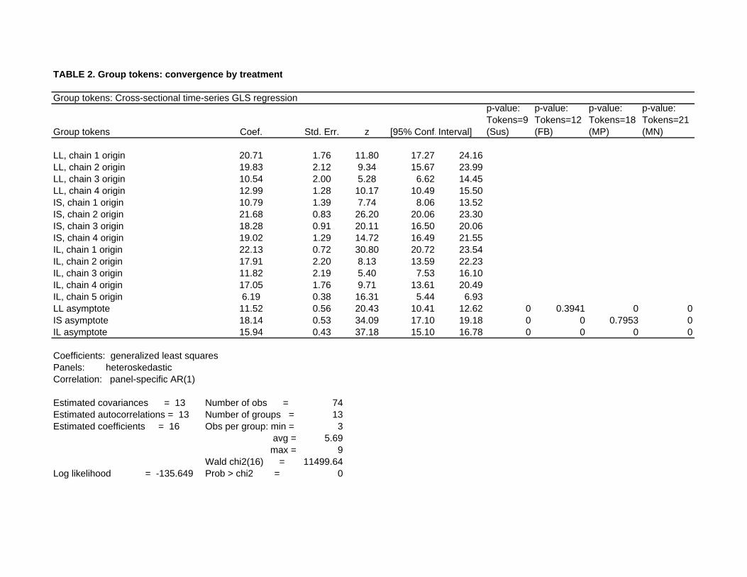
TABLE 2. Group tokens: convergence by treatment

Group tokens: Cross-sectional time-series GLS regression

Group tokens Coef. Std. Err. z [95% Conf. Interval]

p-value: Tokens=9 (Sus)

p-value: Tokens=12 (FB)

p-value: Tokens=18 (MP)

p-value: Tokens=21 (MN)

LL, chain 1 origin 20.71 1.76 11.80 17.27 24.16LL, chain 2 origin 19.83 2.12 9.34 15.67 23.99LL, chain 3 origin 10.54 2.00 5.28 6.62 14.45LL, chain 4 origin 12.99 1.28 10.17 10.49 15.50IS, chain 1 origin 10.79 1.39 7.74 8.06 13.52IS, chain 2 origin 21.68 0.83 26.20 20.06 23.30IS, chain 3 origin 18.28 0.91 20.11 16.50 20.06IS, chain 4 origin 19.02 1.29 14.72 16.49 21.55IL, chain 1 origin 22.13 0.72 30.80 20.72 23.54IL, chain 2 origin 17.91 2.20 8.13 13.59 22.23IL, chain 3 origin 11.82 2.19 5.40 7.53 16.10IL, chain 4 origin 17.05 1.76 9.71 13.61 20.49IL, chain 5 origin 6.19 0.38 16.31 5.44 6.93LL asymptote 11.52 0.56 20.43 10.41 12.62 0 0.3941 0 0IS asymptote 18.14 0.53 34.09 17.10 19.18 0 0 0.7953 0IL asymptote 15.94 0.43 37.18 15.10 16.78 0 0 0 0

Coefficients: generalized least squaresPanels: heteroskedasticCorrelation: panel-specific AR(1)

Estimated covariances = 13 Number of obs = 74Estimated autocorrelations = 13 Number of groups = 13Estimated coefficients = 16 Obs per group: min = 3

avg = 5.69max = 9

Wald chi2(16) = 11499.64Log likelihood = -135.649 Prob > chi2 = 0

TABLE 3. Stock: convergence by treatment

Cross-sectional time-series FGLS regression

Stock Coef. Std. Err. z [95% Conf. Interval]

p-value: Stock=34.3 (Sus)

p-value: Stock=42.9 (FB)

p-value: Stock=60 (MP)

p-value: Stock=68.9 (MN)

Origin 43.13 1.13 38.25 40.92 45.34LL asymptote 45.85 3.01 15.23 39.95 51.75 0.0001 0.327 0 0IS asymptote 65.84 1.09 60.35 63.70 67.98 0 0 0 0.005IL asymptote 60.53 2.59 23.36 55.45 65.61 0 0 0.837 0.0012


Estimated covariances = 13 Number of obs = 74Estimated autocorrelations = 13 Number of groups = 13Estimated coefficients = 4 Obs per group: min = 3 avg = 5.692308 max = 9 Wald chi2(16) = 8632.2Log likelihood = -215.061 Prob > chi2 = 0.0000

TABLE 4. Recommended group tokens: convergence by treatment

Cross-sectional time-series FGLS regression

Recommended group tokens Coef. Std. Err. z [95% Conf. Interval]

p-value: Tokens=9 (Sus)

p-value: Tokens=12 (FB)

p-value: Tokens=18 (MP)

p-value: Tokens=21 (MN)

LL, chain 1 origin 18.99 0.97 19.60 17.09 20.88LL, chain 2 origin 14.87 2.83 5.26 9.33 20.41LL, chain 3 origin 10.73 0.56 19.09 9.63 11.83LL, chain 4 origin 12.09 0.95 12.77 10.23 13.94IS, chain 1 origin 8.77 2.67 3.28 3.53 14.00IS, chain 2 origin 21.57 0.04 553.61 21.49 21.64IS, chain 3 origin 13.77 0.99 13.86 11.82 15.71IS, chain 4 origin 18.13 1.13 16.09 15.92 20.34IL, chain 1 origin 18.15 1.60 11.36 15.02 21.28IL, chain 2 origin 16.94 0.99 17.05 14.99 18.88IL, chain 3 origin 8.32 1.72 4.83 4.94 11.69IL, chain 4 origin 16.33 2.17 7.52 12.08 20.59IL, chain 5 origin 4.49 0.56 8.08 3.40 5.58LL asymptote 11.48 0.33 34.81 10.84 12.13 0 0.1161 0 0IS asymptote 17.21 0.05 319.96 17.11 17.32 0 0 0 0IL asymptote 14.19 0.52 27.06 13.16 15.22 0 0 0 0


Estimated covariances = 13 Number of obs = 72Estimated autocorrelations = 13 Number of groups = 13Estimated coefficients = 16 Obs per group: min = 3 avg = 5.538462

max = 9 Wald chi2(16) = 1766836Log likelihood = -119.186 Prob > chi2 = 0

Figure 1: An example of subject payoff table

Payoffs with Group Tokens = 21 in each series

Your Tokens Payoff Level 1 2 3 4 5 6 7 8 9 10 11Payoff in this series 1394 1 287 521 703 833 911 937 911 833 703 521Payoff in the next series 910 -483 -197 37 219 349 427 453 427 349 219 37Payoff in two series ahead 765 -628 -342 -108 74 204 282 308 282 204 74 -108Payoff in three series ahead 722 -671 -385 -151 31 161 239 265 239 161 31 -151Payoff in four series ahead 709 -684 -398 -164 18 148 226 252 226 148 18 -164

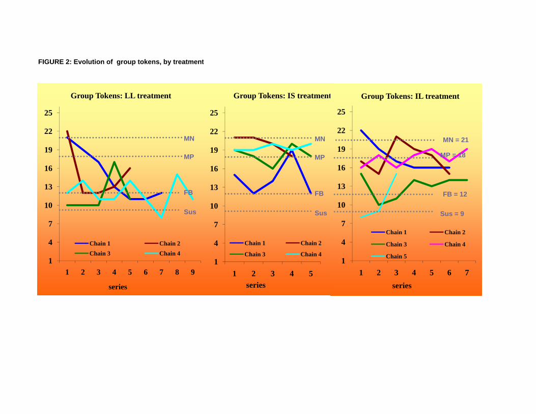
FIGURE 2: Evolution of group tokens, by treatment

Group Tokens: LL treatment Group Tokens: IS treatment Group Tokens: IL treatment

19

22

25

Group Tokens: LL treatment

MN

19

22

25

Group Tokens: IS treatment

MN

19

22

25

Group Tokens: IL treatment

MN = 21

13

16

19

22

25


MP

FB

MN

13

16

19

22

25


MP

FB

MN

13

16

19

22

25


MP = 18

FB = 12

MN = 21

4

7

10

13

16

19

22

25


Chain 1 Chain 2

Sus

MP

FB

MN

4

7

10

13

16

19

22

25


Chain 1 Chain 2

Sus

MP

FB

MN

4

7

10

13

16

19

22

25


Chain 1 Chain 2

Ch i 3 Ch i 4

Sus = 9

MP = 18

FB = 12

MN = 21

1

4

7

10

13

16

19

22

25

1 2 3 4 5 6 7 8 9

series


Chain 1 Chain 2Chain 3 Chain 4

Sus

MP

FB

MN

1

4

7

10

13

16

19

22

25

1 2 3 4 5series


Chain 1 Chain 2

Chain 3 Chain 4

Sus

MP

FB

MN

1

4

7

10

13

16

19

22

25

1 2 3 4 5 6 7series


Chain 1 Chain 2

Chain 3 Chain 4

Chain 5

Sus = 9

MP = 18

FB = 12

MN = 21

1

4

7

10

13

16

19

22

25

1 2 3 4 5 6 7 8 9

series



Sus

MP

FB

MN

1

4

7

10

13

16

19

22

25

1 2 3 4 5series


Chain 1 Chain 2

Chain 3 Chain 4

Sus

MP

FB

MN

1

4

7

10

13

16

19

22

25

1 2 3 4 5 6 7series


Chain 1 Chain 2

Chain 3 Chain 4

Chain 5

Sus = 9

MP = 18

FB = 12

MN = 21

FIGURE 3: Evolution of stock, by treatment

70Stock Level: LL treatment

MN =

70Stock Level: IS treatment

MN = 70

Stock Level: IL treatment

MN = 68.6

55

60

65


MP =

MN =

55

60

65


MP =

MN =

55

60

65

70Stock Level: IL treatment

MP = 60

MN = 68.6

40

45

50

55

60

65


MP =

FB =

MN =

40

45

50

55

60

65


MP =

FB =

MN =

40

45

50

55

60

65


MP = 60

FB = 42.9

MN = 68.6

30

35

40

45

50

55

60

65


Sus

MP =

FB =

MN =

30

35

40

45

50

55

60

65


Sus

MP =

FB =

MN =

30

35

40

45

50

55

60

65


Ch i 1 Ch i 2 Ch i 3

Sus =34.3

MP = 60

FB = 42.9

MN = 68.6

25

30

35

40

45

50

55

60

65

70

1 2 3 4 5 6 7 8 9series

Stock Level: LL treatment

Chain 1 Chain 2 Chain 3 Chain 4

Sus

MP =

FB =

MN =

25

30

35

40

45

50

55

60

65

70

1 2 3 4 5series

Stock Level: IS treatment


Sus

MP =

FB =

MN =

25

30

35

40

45

50

55

60

65

70

1 2 3 4 5 6 7series


Chain 1 Chain 2 Chain 3

Chain 4 Chain 5

Sus =34.3

MP = 60

FB = 42.9

MN = 68.6

25

30

35

40

45

50

55

60

65

70

1 2 3 4 5 6 7 8 9series

Stock Level: LL treatment

Chain 1 Chain 2 Chain 3 Chain 4

Sus

MP =

FB =

MN =

25

30

35

40

45

50

55

60

65

70

1 2 3 4 5series

Stock Level: IS treatment


Sus

MP =

FB =

MN =

25

30

35

40

45

50

55

60

65

70

1 2 3 4 5 6 7series



Chain 4 Chain 5

Sus =34.3

MP = 60

FB = 42.9

MN = 68.6

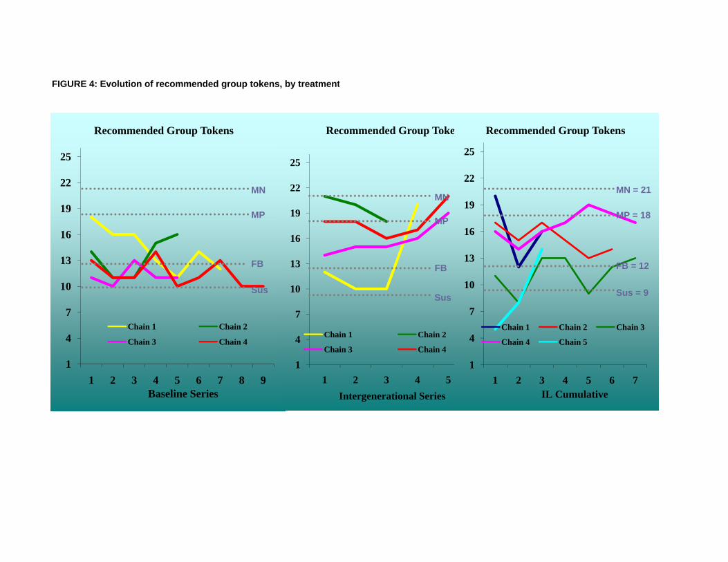
FIGURE 4: Evolution of recommended group tokens, by treatment

Recommended Group Tokens Recommended Group Tokens Recommended Group Tokens

22

25

Recommended Group Tokens

MN 22

25


MN19

22

25


MN = 21

13

16

19

22

25


MP

FB

MN

13

16

19

22

25


MP

FB

MN

13

16

19

22

25


MP = 18

FB = 12

MN = 21

`

7

10

13

16

19

22

25


Chain 1 Chain 2

Sus

MP

FB

MN

7

10

13

16

19

22

25


Sus

MP

FB

MN

7

10

13

16

19

22

25



Sus = 9

MP = 18

FB = 12

MN = 21

`

1

4

7

10

13

16

19

22

25

1 2 3 4 5 6 7 8 9Baseline Series


Chain 1 Chain 2

Chain 3 Chain 4

Sus

MP

FB

MN

1

4

7

10

13

16

19

22

25

1 2 3 4 5Intergenerational Series


Chain 1 Chain 2

Chain 3 Chain 4

Sus

MP

FB

MN

1

4

7

10

13

16

19

22

25

1 2 3 4 5 6 7IL Cumulative



Chain 4 Chain 5

Sus = 9

MP = 18

FB = 12

MN = 21

`

1

4

7

10

13

16

19

22

25

1 2 3 4 5 6 7 8 9Baseline Series


Chain 1 Chain 2

Chain 3 Chain 4

Sus

MP

FB

MN

1

4

7

10

13

16

19

22

25

1 2 3 4 5Intergenerational Series


Chain 1 Chain 2

Chain 3 Chain 4

Sus

MP

FB

MN

1

4

7

10

13

16

19

22

25

1 2 3 4 5 6 7IL Cumulative



Chain 4 Chain 5

Sus = 9

MP = 18

FB = 12

MN = 21

`

FIGURE 5 E l ti f b l d i LL t t t Ch i 2FIGURE 5: Evolution of verbal advice, LL treatment, Chain 2

S eries S u b jec t Ad vise

S eries 1 1 6 as n ext to ken o rd er


S eries 1 1 6 as n ext to ken o rd er2 w e s ta rted o u t rea lly h ig h th is p ast o n e . m ayb e w e can g o lo w er fo r th e n ext tria ls .

3 S ta rt w ith sm all o rders an d g rad ua lly o rd er m o re fo r each subseq u ent tria l. T h e lo ss w e take ea rly w ill g ive u s b ig g er p ayo ffs in th e la te r series .

S i 2 1 I i h ID #3 ' d i i ll d d d ll d i




S eries 2 1 I ag ree w ith ID #3 's ad vice o n s ta rting on sm alle r o rders an d g radua lly o rdering m o re fo r each tria l. I su ffe red fro m a lo ss in th e b eg in n in g , b u t m y p ayo ffs in creased as w e w ent on . Le t'

2 b e tte r, m u ch b ette r. If w e can keep it lo w er o r abou t th e sam e fo r nex t ro u nd th en our p ayo ff w ill b e g rea ter in th e su b seq u en t tria ls .






S eries 3 1 G ood , it seem s to be ge tting be tte r and b e tte r. Le t's keep it a t th e sam e or even lo w er. Le t's ju s t no t go g rea ter

2 H m m ...th e to kens w ere a round th e sam e ba llp ark . M ayb e keep it th e sam e fo r one m o re series th en s ta rt to p u sh o u r lu ck an d s lo w ly in c rease in to ken co u n ts .

3 Le t's s tay w ith th is o rd er o n e m o re ro u n d It g ives u s a g o o d b a lan ce b etw een p ayo u t








3 L e t's s tay w ith th is o rder one m o re ro u nd . It g ives u s a go od b a lance b e tw een payout an d up p ing th e payo ff leve l fo r th e nex t series .

S eries 4 1 P ayo ff d id in crease , bu t I th in k w e shou ld in crease o u r to ken ra th er th an s tay a t 4 . Le t's try in creas ing it a b it

2 I say s lo w ly u p th e to ken co unt…3 T he b ene fit from 4 to 5 is on ly a 100 p o in t d iffe ren ce (50 cen ts ) so le t's s tay w ith 4 .








3 L e t's s tay w ith th is o rder one m o re ro u nd . It g ives u s a go od b a lance b e tw een payout an d up p ing th e payo ff leve l fo r th e nex t series .

S eries 4 1 P ayo ff d id in crease , bu t I th in k w e shou ld in crease o u r to ken ra th er th an s tay a t 4 . Le t's try in creas ing it a b it

2 I say s lo w ly u p th e to ken co unt…3 The bene fit from 4 to 5 is on ly a 100 po in t d iffe ren ce (50 cen ts ) so le t's s tay w ith 4 .

S eries 5 1 Le t's ju s t s tay a t 4 ...doesn 't lo ok like it's in creas ing b y m u ch . 4 w ou ld be th e best to ken o rder. 4 everyone !

2 ...I do n 't kn ow w h at to say no w . W e seem to be do in g w h a ts bes t.

FIGURE 6 E l ti f b l d i IS t t t Ch i 4FIGURE 6: Evolution of verbal advice, IS treatment, Chain 4

Series Subject Advise

Series 1 4 For me I try to choose the tokens which has the highest payoff.5


Series 1 4 For me I try to choose the tokens which has the highest payoff.56 the next set you should choose a low amount of tokens so your payoff level will increase. In the long

run, as the pay off level increases, you will have a higher payoff schedule. I chose 4 because its not too low and not too high but just right.




Series 2 4 Do not choose a number beyond 6. Otherwise, our total payoff will decrease. 5 The greatest payoff calculated against the results for the subsequent group is 66 for maxmin payoff for your series, but the payoff decreases for the later series

Series 3 4 Do not choose higher than 5 Otherwise your optimal payoff will decrease





Series 3 4 Do not choose higher than 5. Otherwise your optimal payoff will decrease.5 keep it fairly low until later rounds6 choose 7

Series 4 4 never go beyond 5 to save your future generations






Series 4 4 never go beyond 5 to save your future generations5 for everyone's best6 choose 6 b/c you make money plus earn more money in the following rounds.

Series 5 4 go between 6 and 8 tokens to gain max payoff and prediction bonus5 for your own benefit, choose the maximal payoff, ie 7; the rest is not worth considering, it's just a

diversion






Series 4 4 never go beyond 5 to save your future generations5 for everyone's best6 choose 6 b/c you make money plus earn more money in the following rounds.

Series 5 4 go between 6 and 8 tokens to gain max payoff and prediction bonus5 for your own benefit, choose the maximal payoff, ie 7; the rest is not worth considering, it's just a

diversion.6 Get the most out of it NOW!

FIGURE 7: Evolution of verbal advice, IL treatment, Chain 4

Series Subject Advice

Series 1 1 PLEASE try either try 3 or 4...dont kill the group payoff, which will affect all of you when it continues further it will affect your individual payoff too. I chose 4 for the first trial and then I stayed around that number, I wanted to stay low because I thought that the actual Payoff Group level would increase if th b f t k d d lthe number of tokens ordered was low.

23 the lower the numbers, the higher the payoff in the later series

Series 2 1 Choose Low so that we can increase the payoff level!2 stay low. 3 or 4 will keep it going. please!3 th l th b th hi h th ff i ill b l t3 the lower the number, the higher the payoff series will be later...

Series 3 1 ok, lets all go low now. if we do this together, we will get better payoff until the end!!2 bid high3 there are three trials,so if we choose a low number between 2 and 5 for the next series, then we can

increase our payoff AND our payoff levels. We ALL can GET MORE MONEY at the end of this

Series 4 1 Go with the lower orders, it'll help out later. for real.2 lower the better3 keep the numbers lower to get a higher payoff

Series 5 1 keep it at 3 or 4 please! if people get greedy, then the token prediction will be off. and people will lose moneymoney.

2 4 The number from 2 to 5 is better. Dont go to higher number.3 I picked 4, so that my own payoff was somewhat average. Overall, a lower number increases the

group payoff in the end.Series 6 1 Please please please, dont be greedy now. With a 75% chance that the experiment will continue,

odds are pretty good that it will keep going The lower the pay off that the next group can get will hurtodds are pretty good that it will keep going. The lower the pay off that the next group can get will hurt your total income in the long run.

2 If you keep the number low, it will pay off in the end. If you are greedy, then only you benefit and no one else...but it will come back to you later.

3 Keep it BELOW five in the first series. In the last series, BID HIGH. DON'T DO IT BEFORE THEN.

Series 7 1 Please keep the your token around 3-4.Series 7 1 Please keep the your token around 3 4.2 try to hit low orders first 3 pick a middle number like 5 or 6 but assume that others will pick a low number (they will want to

ensure better payoff levels)

Experimental Instructions (IL)

Introduction

You are about to participate in an experiment in the economics of decision making in which you will

earn money based on the decisions you make. All earnings you make are yours to keep and will be

paid to you IN CASH at the end of the experiment. During the experiment all units of account will

be in experimental dollars. Upon concluding the experiment the amount of experimental dollars you

receive as payoff will be converted into dollars at the conversion rate of US $1 per experimental

dollars, and will be paid to you in private.

Do not communicate with the other participants except according to the specific rules of the exper-

iment. If you have a question, feel free to raise your hand. An experimenter will come over to you and

answer your question in private.

In this experiment you are going to participate in a decision process along with several other

participants. From now on, you will be referred to by your ID number. Your ID number will be

assigned to you by the computer.

Decisions and Earnings

Decisions in this experiments will occur in a number of decision series. Decisions in each decision

series are made within groups of 3 participants each. A number of these groups form a chain. At the

beginning of your decision series, you will be assigned to a decision group with 2 other participant(s).

You will not be told which of the other participants are in your decision group.

You and other participants in your group will make decisions in the current decision series. This

decision series may have been preceded by the previous series, where decisions were made by your

predecessor group in the chain. Likewise, your decision series may be followed by the next decision

series, where decisions will be made by your follower group in the chain. None of the participants in

the current session are in the predecessor or the follower group in your chain.

In this decision series, you will be asked to order between 1 and 11 tokens. All participants in your

group will make their orders at the same time. You payoff from each series will depend on two things:

(1) the current payoff level for your group, and (2) the number of tokens you order. The higher is the

group payoff level for the series, the higher are your payoffs in this series. All members of your group

have the same group payoff level in this series.

Given a group payoff level, the relationship between the number of tokens you order and your payoff

may look something like this:

PAYOFF SCHEDULE IN THIS SERIES; GROUP PAYOFF LEVEL: 1394

Your token order 1 2 3 4 5 6 7 8 9 10 11Payoff in this series 1 287 521 703 833 911 937 911 833 703 521

1

For example, the table above indicates that the group payoff level in this series is 1394. At this

level, if you choose to order 5 tokens, then your payoff will be 833 experimental dollars.

The group payoff level for your decision series will be given to you by the computer. This payoff level

may be the result of decisions of participants in the predecessor group in your chain in the previous series.

Likewise, the payoff level for the follower group in your chain in the next series will depend on your group’s

total token order in this series. The follower’s group payoff level in the next series may increase if the

number of tokens ordered by your group in this series is low; The follower’s group payoff level in the

next series may decrease if the number of tokens ordered by the group in this series is high; For some

group token order, your follower’s group payoff level in the next series may be the same as your group’s

payoff level in this series.

Example 1 To illustrate how payoff schedules in your chain may change from series to series,

depending on your group orders, consider the attachment called “Example 1 Scenarios”. Suppose, as in

this attachment, that your group has a payoff level of 1394 in the current series. The table and figure

A1 illustrate how the payoffs change from series to series for the groups in your chain, if the group

order the sum of 3 tokens in each series. The table shows the group payoff level will increase from 1394

in this series to 1878 in the next series, resulting in increased payoffs from token orders. For example,

if you order 1 token, your payoff will be 1 experimental dollar in this series, but in the next series your

follower’s payoff from the same order will increase to 485 experimental dollars. The table also shows

that if the group order is again 3 tokens in the next series, the group payoff level will further increase

in the series after next. Similarly, the table demonstrates the payoff changes in the future series up to

three series ahead. The graph illustrates.

When making token orders, you will be given a calculator which will help you estimate the effect of

your and the other participants’ token choices on the follower groups payoff levels in the future series.

In fact, you will have to use this calculator before you can order your tokens.

TRY THE CALCULATOR ON YOUR DECISION SCREEN NOW. In the calculator box,

enter ”1” for your token order, and ”2” for the sum of the other participants’ orders. (The group tokens

will be then equal to 3.) The ”Calculator Outcome” box will show the changes in the payoff levels and

the actual payoffs from the current series to the next and up to four series ahead, if these token orders

are chosen in every series. Notice how the payoff levels and the actual payoffs increase from series to

series.

Consider now the table and figure A4. They illustrate how payoff levels change from series to series

if your group and the follower groups in your chain order the total of 30 tokens in each series. Suppose,

for example, that you order 11 tokens in this series. The table shows that, given the current payoff

level, your payoff will be 521 experimental dollar in this series, but in the next series your follower’s

payoff from the same order will be -446 experimental dollars. (This is because the group payoff level

2

will decrease from 1394 in this series to 427 in the next series.) Again, the table and the graph illustrate

how the payoffs change in the future series up to three series ahead, assuming that the total group order

stays at 30 tokens in each series.

TRY THE CALCULATOR WITH THE NEW NUMBERS NOW. In the calculator box, enter

”11” for your token order, and ”19” for the sum of the other participants’ orders. (The group tokens

will be then equal to 30.) The ”Calculator Outcome” box will again show the changes in the payoff

levels and the actual payoffs from the current series to the next and up to four series ahead, given the

new token orders. Notice how the payoff levels and the actual payoffs decrease from series to series.

Now try the calculator with some other numbers.

After you practice with the calculator, ENTER A TOKEN ORDER IN THE DECISION BOX.

The decision box is located on your decision screen below the calculator box.

Predictions Along with making your token order, you will be also asked to predict the sum of

token orders by other participants in your group. You will get an extra 50 experimental dollars for

an accurate prediction. Your payoff from prediction will decrease with the difference between your

prediction and the actual tokens ordered by others in your group. The table below explains how you

payoff from prediction depends on how accurate your prediction is.

PAYOFF FROM PREDICTIONS

Difference between predicted andactual sum of others’ tokens 0 2 4 6 8 10 12 14 16 18 20

Your Payoff from Prediction 50 50 48 46 42 38 32 26 18 10 0

PLEASE ENTER A PREDICTION INTO THE DECISION BOX NOW.

Results After all participants in your group make their token orders and predictions, the computer

will display the “Results” screen, which will inform you about your token order, the sum of the other

participants’ tokens, and your total payoff in this series. The total payoff equals the sum of your payoff

from token order and your payoff from prediction. The results screen will also inform you about the

change in the payoff levels from this series to the next series, and display the corresponding payoff

schedules.

Trials You will be given three independent decision trials to make your token orders and predictions

in this series. The payoff levels for your group will stay the same across the trials of the series. At the

end of the series, the computer will randomly choose one of these three trials as a paid trial. This paid

trial will determine the earnings for the series, and the payoff level for your follower group in the next

series. All other trials will be unpaid. At the end of the series, the series results screen will inform you

which trial is chosen as the paid trial for this series.

3

Advice from the previous series and for the next series Before making token orders in your

decision series, you will be given a history of token orders and advice from the participants in the

predecessor groups in your chain, suggesting the number of tokens to order. At the end of your decision

series, each participant in your group will be asked to send an advice message to the participants in

the follower group in your chain. This will conclude a given series.

PLEASE ENTER AN ADVICE (A SUGGESTED NUMBER OF TOKENS AND A VER-

BAL ADVICE) NOW.

Continuation to the next decision series Upon conclusion of the decision series, we will roll

an eight-sided die to determine whether the experiment ends with this series or continues to the next

series with the follower group. If the die comes up with a number between 1 and 6, then the experiment

continues to the next series. If the die shows number 7 or 8, then the experiment stops. Thus, there

are THREE CHANCES OUT OF FOUR that the experiment continues to the next series, and ONE

CHANCE OUT OF FOUR that the experiments stops.

If the experiment continues, the next series that follows will be identical to the previous one except

for the possible group payoff level change, depending on the token orders by your group in this series,

as is explained above. The decisions in the next series will be made by the participants in the follower

group in your chain.

Practice Before making decisions in the paid series, all participants will go through 5-series practice,

with each practice series consisting of one trial only. You will receive a flat payment of 10 dollars for

the practice.

Total payment Your total payment (earning) in this experiment will consist of two parts: (1) The

flat payment for the practice, which you will receive today; plus (2) the sum of yours and your followers’

series payoffs, starting from your series and including all the follower series in your chain. This payment

will be calculated after the last series in your chain ends. We will invite you to receive the latter part

of your payment as soon as the experiment ends.

If you have a question, please raise your hand and I will come by to answer your question.

ARE THERE ANY QUESTIONS?

4

Frequently asked questions

• What is the difference between a trial and a series?

Each series consists of three decision trials. One of the decision trials is then randomly chosen

by the computer to determine your payoffs in the series.

• What does my payoff in this series depend upon?

It depends upon your GROUP PAYOFF LEVEL in this series, and YOUR TOKEN ORDER.

• What is the group payoff level?

It is a positive number that is related to the payoffs you can get from token orders in the series.

The higher is the group payoff level, the higher is the payoff you get from any token order.

• Does my payoff in a series depend upon other participants’ token orders in this series?

No. Given your group payoff level in a series, your payoff in this series is determined only by

your own tokens order.

• Why do the total group tokens matter?

Because THEY AFFECT THE PAYOFF LEVEL IN THE NEXT SERIES for the follower group

in your chain. The higher is the group tokens in this series, the lower will be the group payoff

level in the next series.

• How many series are there in this experiment?

The number of series will be determined by a random draw. There will be 3 OUT OF 4 CHANCES

that each series will continue to the next series, and 1 OUT OF 4 CHANCE that the experiment

will stop after this series. We will roll a die at the end of each series to determine the outcome.

5

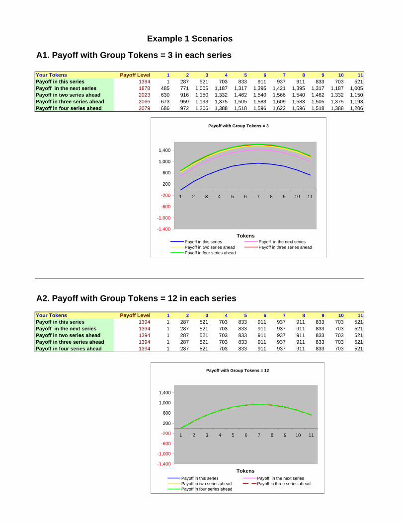
Example 1 Scenarios

A1. Payoff with Group Tokens = 3 in each series

Your Tokens Payoff Level 1 2 3 4 5 6 7 8 9 10 11

Payoff in this series 1394 1 287 521 703 833 911 937 911 833 703 521Payoff in the next series 1878 485 771 1,005 1,187 1,317 1,395 1,421 1,395 1,317 1,187 1,005Payoff in two series ahead 2023 630 916 1,150 1,332 1,462 1,540 1,566 1,540 1,462 1,332 1,150Payoff in three series ahead 2066 673 959 1,193 1,375 1,505 1,583 1,609 1,583 1,505 1,375 1,193Payoff in four series ahead 2079 686 972 1,206 1,388 1,518 1,596 1,622 1,596 1,518 1,388 1,206



Payoff in this series 1394 1 287 521 703 833 911 937 911 833 703 521Payoff in the next series 1394 1 287 521 703 833 911 937 911 833 703 521Payoff in two series ahead 1394 1 287 521 703 833 911 937 911 833 703 521Payoff in three series ahead 1394 1 287 521 703 833 911 937 911 833 703 521Payoff in four series ahead 1394 1 287 521 703 833 911 937 911 833 703 521

Payoff with Group Tokens = 3

-1,400

-1,000

-600

-200

200

600

1,000

1,400

1 2 3 4 5 6 7 8 9 10 11

TokensPayoff in this series Payoff in the next seriesPayoff in two series ahead Payoff in three series aheadPayoff in four series ahead


-1,400

-1,000

-600

-200

200

600

1,000

1,400

1 2 3 4 5 6 7 8 9 10 11


Example 1 Scenarios



Payoff in this series 1394 1 287 521 703 833 911 937 911 833 703 521Payoff in the next series 910 -483 -197 37 219 349 427 453 427 349 219 37Payoff in two series ahead 765 -628 -342 -108 74 204 282 308 282 204 74 -108Payoff in three series ahead 722 -671 -385 -151 31 161 239 265 239 161 31 -151Payoff in four series ahead 709 -684 -398 -164 18 148 226 252 226 148 18 -164



Payoff in this series 1394 1 287 521 703 833 911 937 911 833 703 521Payoff in the next series 427 -966 -680 -446 -264 -134 -56 -30 -56 -134 -264 -446Payoff in two series ahead 137 -1,256 -970 -736 -554 -424 -346 -320 -346 -424 -554 -736Payoff in three series ahead 50 -1,343 -1,057 -823 -641 -511 -433 -407 -433 -511 -641 -823Payoff in four series ahead 23 -1,370 -1,084 -850 -668 -538 -460 -434 -460 -538 -668 -850


-1,400

-1,000

-600

-200

200

600

1,000

1,400

1 2 3 4 5 6 7 8 9 10 11



-1,400

-1,000

-600

-200

200

600

1,000

1,400

1 2 3 4 5 6 7 8 9 10 11


games with dynamic externalities and climate change experiments …€¦ · games with dynamic...

Documents