games and economic behavior - stanford universityniederle/featherstone.niederl… · ·...

Games and Economic Behavior 100 (2016) 353–375

Contents lists available at ScienceDirect

Games and Economic Behavior

www.elsevier.com/locate/geb

Boston versus deferred acceptance in an interim setting:

An experimental investigation ✩

Clayton R. Featherstone a,∗, Muriel Niederle b,c

a University of Pennsylvania, The Wharton School, 3620 Locust Walk – SHDH 1352, Philadelphia, PA 19104, United Statesb Stanford University, Department of Economics, United Statesc NBER, United States

a r t i c l e i n f o a b s t r a c t

Article history:Received 16 July 2013Available online 14 October 2016

JEL classification:C78C90D47D82

Keywords:School choice mechanismsMarket designExperimental economicsMatching theory

While much of the school choice literature advocates strategyproofness, recent research has aimed to improve efficiency using mechanisms that rely on non-truthtelling equilibria. We address two issues that arise from this approach. We first show that even in simple environments with ample feedback and repetition, agents fail to reach non-truthtelling equilibria. We offer another way forward: implementing truth-telling as an ordinal Bayes–Nash equilibrium rather than as a dominant strategy equilibrium. We show that this weaker solution concept can allow for more efficient mechanisms in theory and provide experimental evidence that this is also the case in practice. In fact, truth-telling rates are basically the same whether truthtelling is implemented as an ordinal Bayes–Nash equilibrium or a dominant strategy equilibrium. This provides a proof-of-concept that ordinal Bayes–Nash design might provide a middle path, achieving efficiency gains over strategy-proof mechanisms without relying on real-life agents playing a non-truth-telling equilibrium.

© 2016 Elsevier Inc. All rights reserved.

1. Introduction

Former Boston Public Schools superintendent Thomas Payzant described the rationale for switching away from a ma-nipulable choice mechanism quite succinctly: “A strategy-proof algorithm ‘levels the playing field’ by diminishing the harm done to parents who do not strategize or do not strategize well.”1,2 This quote highlights two main assumptions implicit in much of the school choice literature. The first is that a significant fraction of parents will strategize poorly if faced with a situation where truth-telling is sub-optimal. The second is that if truth-telling is not a dominant strategy, then parents might fail to submit preferences truthfully. In this paper, we present an experiment that investigates both of these assump-

✩ This paper has also circulated under the titles “Improving on Strategy-proof School Choice Mechanisms: An Experimental Investigation”, “School Choice Mechanisms under Incomplete Information: An Experimental Investigation”, and “Ex Ante Efficiency in School Choice Mechanisms: An Experimental Investigation”.

* Corresponding author.E-mail address: [email protected] (C.R. Featherstone).

1 A school choice mechanism maps students’ reported preferences over schools to lotteries over possible allocations of students to schools. A strategy-proof school choice mechanism admits truthful preference revelation as a weakly dominant strategy. A non-strategy-proof mechanism is also called manipulable.

2 For more about Boston Public Schools’ decision to adopt a deferred acceptance assignment system, see Abdulkadiroglu et al. (2005b) and Abdulkadiroglu et al. (2006).

http://dx.doi.org/10.1016/j.geb.2016.10.0050899-8256/© 2016 Elsevier Inc. All rights reserved.

http://dx.doi.org/10.1016/j.geb.2016.10.005

http://www.ScienceDirect.com/

http://www.elsevier.com/locate/geb

mailto:[email protected]

http://dx.doi.org/10.1016/j.geb.2016.10.005

http://crossmark.crossref.org/dialog/?doi=10.1016/j.geb.2016.10.005&domain=pdf

354 C.R. Featherstone, M. Niederle / Games and Economic Behavior 100 (2016) 353–375

tions in the context of two common school choice mechanisms: the strategy-proof Deferred Acceptance mechanism (“DA”) and the non-strategy-proof, “immediate acceptance” mechanism once used in Boston (“Boston”).3

The Boston mechanism is quite popular, presumably because it maximizes the number of students that receive their re-ported first choice.4 However, it also provides participants with incentives to manipulate their preference reports, and in fact, a large number of experiments have confirmed that students do indeed deviate from truth-telling (Chen and Sönmez, 2006;Pais and Pintér, 2008; Calsamiglia et al., 2010).5 These papers mainly focus on determining what rules-of-thumb par-ticipants use when choosing their strategically manipulated preference reports. While Boston Public Schools has re-placed the Boston mechanism with strategy-proof DA, several recent papers (Abdulkadiroglu et al., 2011; Miralles, 2009;Abdulkadiroglu et al., 2015) have demonstrated that non-truth-telling equilibria under the old Boston mechanism can yield significant efficiency gains. For example, Abdulkadiroglu et al. (2011) shows in a stylized environment that the Boston mech-anism can sustain a generically non-truth-telling equilibrium that dominates the truth-telling DA equilibrium by allowing students to better express their cardinal preferences.6 This raises a new question that current experiments fail to address, namely whether students would play close enough to the equilibrium prediction in a Boston mechanism for these gains to be realized.7 Existing experiments cannot address this question, as they generally did not give participants sufficient information to calculate the equilibrium.8

The first part of our experiment tries to close this gap by considering a very simple incomplete information environ-ment that has a unique, non-truth-telling equilibrium under the Boston mechanism.9 As theory predicts, students truth-tell under DA. Under Boston, we confirm former results that students do not play truth-telling strategies. However, even in our simple environment with feedback and repetition, students fail to play the theoretical equilibrium and in general are far from playing a best response. This lines up well with the general finding of the experimental literature on Bayesian games: that subjects have a hard time finding the equilibrium.10 As such, we confirm the worry of Boston Public Schools superin-tendent Thomas Payzant that equilibria that entail untruthful reporting may be difficult to successfully implement in actual school choice problems.

Payzant’s second assumption is that strategy-proofness may be necessary to “level the playing field”. However, dominant-strategy incentive compatibility, while appealing, imposes a strong constraint on design, and it has been shown empirically that this constraint can come with costs.11 If we could successfully implement truth-telling in a weaker way, then we would open the door to the possibility of leveling the playing field with non-strategy-proof designs that are customized to induce truth-telling in particular environments.

In the second part of the experiment, we try to show that this could work by considering an environment in which truth-telling is an ordinal Bayes–Nash equilibrium under the non-strategy-proof Boston (and of course, a dominant-strategy equilibrium under DA).12 In this environment, we show that participants truth-tell when it is an equilibrium to do so, whether it is implemented as an ordinal Bayes–Nash equilibrium or a dominant strategy equilibrium.13 Indeed, truth-telling rates turn out to be high and not statistically different across the two mechanisms. Furthermore, we empirically observe

3 DA is currently used in New York City (Abdulkadiroglu et al., 2005a, 2009) and Boston (Abdulkadiroglu et al., 2005b, 2006); Boston, or a close variant, is or has been used in Charlotte-Mecklenburg (North Carolina), Lee County (Florida), Minneapolis, and Seattle (Abdulkadiroglu and Sönmez, 2003). These are, of course, non-exhaustive lists.

4 Mechanisms like Boston are also popular in two-sided markets, see e.g. Roth (1991). While the Boston mechanism maximizes the number of students that receive the school they ranked as their first choice, it does not necessarily maximize the number of students that receive their first or second choice. For an investigation on mechanisms that seek to directly optimize the distribution of ranks received by students, see Featherstone (2016).

5 See Calsamiglia et al. (2011) and Chen and Sönmez (2011) for comments on the data analysis in Chen and Sönmez (2006).6 Troyan (2012) suggests an extension that deals with more complex priority structures.7 Abdulkadiroglu et al. (2006) provide suggestive evidence that some participants in Boston may not have manipulated their preference list in an optimal

way.8 In Pais and Pintér (2008), students can calculate the equilibrium under the full information treatment, but not under their treatments with less

information. The paper does not however address the extent to which students play equilibrium.9 In our experiments, students know their own preferences, but only the distribution from which other students’ preferences are drawn. In one of the

experimental environments, this distribution is degenerate; hence, each student actually knows the true preferences of the other students. Students also know the distribution of lottery tie-breaker draws, but not the realization.10 The general finding in the experimental literature on the implementation of Bayes–Nash equilibria that involve misreporting of preferences is that

the behavior of participants is not close to equilibrium play. See, for example, Featherstone and Mayefsky (2015), Fragiadakis and Troyan (2015), and the summary of work in auctions in the old experimental handbook (Kagel and Roth, 1995, Chapter 8), the new experimental handbook (Kagel and Roth, 2016, Chapter 10 by Kagel and Levin), and in Kagel and Levin’s book on the winner’s curse (Kagel and Levin, 2009).11 Theoretically, dominant-strategy incentive compatibility imposes an incentive compatibility constraint at every possible strategy profile. This is a larger

set of constraints than, say, those required by Bayes–Nash incentive compatibility, which only requires a constraint for each unilateral deviation from the proposed equilibrium. Empirically, Abdulkadiroglu et al. (2009) show that gains from the improvements suggested by Erdil and Ergin (2008) can be significant, but come at the cost of strategy-proofness. See also Kesten and Ünver (2013).12 An ordinal Bayes–Nash equilibrium is a Bayes–Nash equilibrium in which each player’s equilibrium strategy yields an outcome distribution that first-

order stochastically dominates the outcome distributions of all other potential strategies (when all other players are playing equilibrium strategies). See Ehlers and Massó (2007).13 While we believe that only truth-telling ordinal Bayes–Nash equilibria will predict actual behavior, we cannot rule out that even non-truth-telling

ordinal Bayes–Nash equilibria will predict behavior. It this were so, the case for considering non-strategy-proof mechanisms would be stronger, as a weakly larger set of outcomes can be implemented as an ordinal Bayes–Nash equilibrium without the constraint that the equilibrium entails truth-telling. We suspect, however, that non-truth-telling ordinal Bayes–Nash equilibria will not predict actual behavior; for instance, Fragiadakis and Troyan (2015) consider an assignment game with a unique non-truth-telling ordinal Bayes–Nash equilibrium in which subjects play the equilibrium only about 1% of the time.

C.R. Featherstone, M. Niederle / Games and Economic Behavior 100 (2016) 353–375 355

that the Boston outcome stochastically dominates the DA outcome. We cannot emphasize enough that this does not imply that Boston is a good school choice mechanism for most environments. We only show that it is a good mechanism for our particular environment. However, this finding does suggest that a mechanism implementing truth-telling as an ordinal Bayes–Nash equilibrium may still “level the playing field” in Payzant’s sense without being formally strategy-proof (i.e. dominant-strategy incentive-compatible). We also show that weakening the solution concept can yield significant efficiency gains.

In the penultimate section of this paper, we investigate this idea further by first providing theoretical intuition for why Boston performs so well in our particular environment and then by considering what sorts of mechanisms might outperform DA in other environments. We do so by considering a simple model in which ordinal preferences are idiosyncratic across students, drawn according to a simple distribution. Students know their own preferences, but only the distribution from which others’ ordinal preferences are drawn. Throughout, we keep students from needing to know anything about the underlying cardinal preferences by focusing on implementing truth-telling as an ordinal Bayes–Nash equilibrium. Ultimately, we show that, from the interim perspective (in which subjects know their own preference, but not the preferences of others), all subjects would prefer to improve upon DA by implementing a few ex post adjustment rules, so long as those rules are only implemented with certain probabilities. These probabilities simultaneously ensure that all subjects are interim better off, and that they all have incentives for truth-telling.

The theory we describe differs from much of the prior literature in two key ways. First, we investigate both efficiency and equilibrium from the interim information set, where agents know their own preferences, but have only incomplete information about others’ preferences. While this view is more common in the two-sided matching literature (Roth and Rothblum, 1999; Kojima and Pathak, 2009), it is less standard in the school choice literature.14 The interim approach may, however, be more realistic when considering the behavior of students. Furthermore, it may be the right way to think about the objective of a school board that wants to maximize efficiency over several cohorts of students and not simply a specific year (and hence a specific set of realized preferences).

Second, we focus on ordinal Bayes–Nash incentive compatibility, which we feel to be the natural solution concept for non-strategy-proof design. Although non-strategy-proof implementation requires some assumption about underlying prefer-ences, ordinal Bayes–Nash equilibrium only requires assumptions about underlying ordinal preferences, which can be easily estimated from reports submitted to a strategy-proof mechanism such as DA. Bayes–Nash equilibrium, although an even weaker solution concept, requires knowledge of the underlying cardinal preferences of students, which are not as easily ascertained. This aspect of our model also highlights the tension between strategy-proof design, in which one mechanism implements truth-telling in all environments, and ordinal Bayes–Nash design, in which the mechanism must be tuned to the environment. The upside to this tuning is the potential for efficiency gains like those we demonstrate in the lab.

In the literature, the closest work to our own is Abdulkadiroglu et al. (2011), which looks at an environment in which all students have the same ordinal preference, but different underlying cardinal preferences. In this environment, the (generi-cally) non-truth-telling Bayes–Nash equilibria of the Boston mechanism yield outcomes that all students interim prefer to that of the truth-telling equilibrium of DA. This result relies on students being sophisticated enough to misreport prefer-ences in a way that best-responds to their knowledge of the population distribution of cardinal preferences. We think of our model as a useful contrast in which ordinal preferences are not perfectly aligned and interim gains come in a truth-telling equilibrium that does not rely on any knowledge of cardinal utility. However, our model does rely on the market designer to tune the mechanism to the underlying ordinal environment.

The rest of the paper is organized as follows. Section 2 introduces the mechanisms and environments used in the experiment and then presents the experimental design. Sections 3 and 4 discuss the results of the experiment. In Section 5, we discuss the intuition of how and when Boston can implement truth-telling, and briefly extend our findings to less symmetric environments. Section 6 concludes.

2. The experimental setup

In the subsections that follow, we introduce the two school choice mechanisms (“Boston” and “Deferred Acceptance”) and the two preference environments (“aligned” and “uncorrelated”) of our 2 × 2 factorial design. Then, we will discuss how our design allows us to address the questions mentioned in the introduction.

2.1. Two school choice mechanisms

Formally, a school choice mechanism is a mapping from students’ reported preferences to a lottery over allocations of students to schools. This mapping induces a preference revelation game for the students. In the mechanisms that we consider, we generate the outcome lotteries by randomizing the inputs to a deterministic algorithm; specifically, each school draws a strict priority ordering over the students from some distribution. In school choice mechanisms, this random process is usually constructed by starting with a weak ordering based on student characteristics and breaking indifferences with a

14 Notable recent exceptions include Ergin and Sönmez (2006), Erdil and Ergin (2008), Abdulkadiroglu et al. (2011), and Troyan (2012).


lottery.15 Note that we could either draw the lottery independently for each school (multiple lotteries) or just once, using the same lottery for all schools (single lottery).16 While the priorities of the schools are codified by law or administrative procedure, students are strategic players.17

We use two mechanisms in the experiment. The first is based on the Deferred Acceptance algorithm (Gale and Shapley, 1962) and has been introduced in Boston and New York City schools (Abdulkadiroglu et al., 2005a, 2005b).

The Deferred Acceptance Algorithm (DA)

Step 1: Students apply to their first choice school. Schools reject the lowest-ranking students in excess of their capacity. All other offers are held temporarily.

Step t: If a student is rejected in Step t − 1, he applies to the next school on his rank-order list. If he has no more schools on his list, he applies nowhere. Schools consider both new offers and the offers held from previous rounds. They reject the lowest ranked students in excess of their capacity. All other offers are held temporarily.

STOP: The algorithm stops when no rejections are issued. Each school is matched to the students it is holding at the end.

Two well known results concerning the revelation game induced by DA are that truth-telling is a weakly dominant strategy (Dubins and Freedman, 1981; Roth, 1982a, 1982b) and that the outcome is stable relative to reported preferences (Gale and Shapley, 1962).18 The second mechanism we consider is based on a specific priority algorithm, first described as the “Boston Algorithm” by Abdulkadiroglu and Sönmez (2003). This mechanism is commonly used in American public school choice (Abdulkadiroglu et al., 2005b) and can be thought of as an immediate acceptance algorithm.

The Boston Algorithm

Step 1: Students apply to their first choice school. Schools reject the lowest-ranking students in excess of their capacity. All other offers are immediately accepted and become permanent matches. School capacities are adjusted accordingly.

Step t: If a student is rejected in Step t − 1, he applies to the next school on his rank-order list. If he has no more schools on his list, he applies nowhere. Schools reject the lowest ranked students in excess of their capacity. All other offers become permanent matches. School capacities are adjusted accordingly.

STOP: The algorithm stops when no rejections are issued.

Note that in contrast to DA, where applications are tentatively held and acceptance is deferred until the end, applications in the Boston algorithm are immediately accepted or rejected at each step. The chance that one might be able to lock in a school over a higher priority student by ranking that school earlier in the algorithm is intuitively why Boston, unlike DA, fails to be strategy-proof.

2.2. Two preference environments

The first environment we consider is the aligned preference environment. In it there are three schools – “Gold”, “Sil-ver”, and “Bronze” – and five students who are either “Top” or “Average”.19 Gold has two seats, while the other schools have only one seat each, and three of the students are Top, while the other two are Average. Each school prefers a Top student to an Average one, and all students prefer Gold to Silver to Bronze. All students also have the same von Neumann–Morgenstern payoffs over schools: 100 for Gold, 67 for Silver, 25 for Bronze, and 0 for being unmatched.20 Each school has an independently drawn uniform lottery to order students of the same priority class. This environment is summarized in Fig. 1.

The matching that results under DA in equilibrium is the unique stable matching: the two Top students with highest lottery draws at Gold get Gold, the other Top gets Silver, and the Average with the highest lottery draw at Bronze gets Bronze, leaving the remaining Average unmatched.

15 For example, in Boston, the weak ordering is based on whether a student is within walking distance or has a sibling at the school in question (Abdulkadiroglu and Sönmez, 2003).16 This distinction was first made in Abdulkadiroglu et al. (2005a).17 A notable exception to this is school choice in New York City, where school principals can strategically report their preferences over students

(Abdulkadiroglu et al., 2005a).18 Relative to strict preferences for both schools and students, an outcome is called stable if it is individually rational and there is no blocking pair (a student

and a school who each prefer each other to their assigned match). See the Appendix for a formal definition.19 In the actual experiment, “Gold”, “Silver”, and “Bronze” were called “Best”, “Second”, and “Third”, respectively. We changed the names to make the

distinction between schools and ranks more clear in the exposition that follows.20 Note that our setup does not depend on there being more students than seats, as it is theoretically equivalent to interpret “No School” as “Undesirable

School”. And in fact, many real-world school matches have the equivalent of Undesirable School: a school in a bad neighborhood where there is effectively no scarcity of seats.


All schools prioritize... All students prefer...Top � Average Gold � Silver � Bronze � Unmatched(Ties broken by lottery) u = 100 67 25 0

3 students 2 students 2 seats 1 seat 1 seat ∞ seats

Fig. 1. The aligned preference environment.

Proposition 2.1. In the aligned preference environment, a profile of strategies is a Bayes–Nash equilibrium of the revelation game induced by DA if and only if it is a member of the family of profiles defined by the following characteristics:

• Top students submit preferences that rank Gold first and Silver second.• Average students submit preferences that declare Bronze acceptable.

Moreover, all equilibria assign the three Top students to Gold and Silver, one Average student to Bronze, and leave the other Average unmatched.

Note that truth-telling is a weakly dominant strategy under DA. Under Boston, the unique stable outcome is not achiev-able in equilibrium when lottery draws are not known21; in fact, when participants are risk-neutral, the pure-strategy Bayes–Nash equilibrium outcome is unstable.

Proposition 2.2. In the aligned preference environment, when students are risk-neutral, a profile of strategies is a pure-strategy Bayes–Nash equilibrium of the revelation game induced by Boston if and only if it is a member of the family of profiles defined by the following characteristics:

• Top students submit preferences that rank Gold first and Bronze second.• Average students submit preferences that rank Silver first.

Moreover, all pure-strategy equilibria assign the three Top students to Gold and Bronze, one Average student to Silver, and leave the other Average unmatched.

The equilibria of Proposition 2.2 entails two types of manipulations, both of which can be implemented as a dropping strategy.22 Top students need to misreport their second choice school, submitting Bronze instead of Silver, that is, they must “skip the middle”. Average students need to misreport their first ranked school, submitting Silver instead of Gold, that is, they must “skip the top”. Note that, in equilibrium, relative to DA, the Average students are in expectation better off, while the Top students are, in expectation, worse off.

The second environment we consider is the uncorrelated preference environment. In it there are five students and four one-seat schools. Student preferences are drawn independently from the uniform distribution over all possible orderings that find all schools acceptable, and likewise, each school has a strict priority based on an independent draw from the uniform distribution over all orderings of the students. In the experiment the payoffs are such that a seat at the highest ranked school yields 110 points, the second highest 90, the third highest 67 and the fourth 25. Being unmatched yields 0 points (recall Footnote 20).

In this environment, both mechanisms admit all agents truth-telling as a Nash equilibrium, but while truth-telling is a weakly dominant strategy under DA, it is only an ordinal Bayes–Nash equilibrium strategy under Boston.23 Under DA, truth-telling is the unique equilibrium in weakly undominated strategies, and under Boston, truth-telling is the unique equilibrium in weakly undominated, anonymous strategies. A strategy is anonymous if the reported rank of a school only depends on its true rank (and not its name).24 Now we state the formal result that all students truth-telling is an ordinal Bayes–Nash equilibrium in both environments, and that this truth-telling is, in some sense, the unique equilibrium in these environments.

Proposition 2.3. In the uncorrelated environment, the revelation game induced by DA admits truth-telling by all students as an ordinal Bayes–Nash equilibrium. Furthermore, this is the unique Bayes–Nash equilibrium.

21 Per Ergin and Sönmez (2006), if the lottery draws at each school are common knowledge, then the equilibrium outcome with Boston is the same as with DA. One set of supporting strategies is as follows: the two Top students with the best lottery numbers at Gold rank it first, the third Top student ranks Silver first, the Average student who has the better lottery number at Bronze ranks it first, and the last Average student submits arbitrary preferences (as he will not receive any school).22 In our context, a dropping strategy submits a rank order that might declare some school(s) unacceptable, but preserves the truthful ordering of those

schools that are declared acceptable.23 For a definition of an ordinal Bayes–Nash equilibrium, see Footnote 12.24 See Definition B.2 for a more formal definition.


Mechanism Boston DA DA

(Single lottery) (Multiple lotteries)

1st choice 0.610 0.500 0.328 (0.328)2nd choice 0.117 (0.727) 0.167 (0.667) 0.222 (0.550)3rd choice 0.055 (0.782) 0.083 (0.750) 0.150 (0.700)4th choice 0.018 (0.800) 0.050 (0.800) 0.100 (0.800)No school 0.200 (1.000) 0.200 (1.000) 0.200 (1.000)

(a) Outcome distributions (CDF in parentheses)

(b) CDF Plots (DA is multiple lotteries, DA-SL is single)

Fig. 2. Theoretical equilibrium outcomes in the uncorrelated environment (100% truth-telling).

Proposition 2.4. In the uncorrelated environment, the revelation game induced by Boston admits truth-telling by all students as an ordinal Bayes–Nash equilibrium. Furthermore, this is the unique Bayes–Nash equilibrium in anonymous strategies.

Note that these propositions are not sensitive to the cardinal utility values that we chose for the uncorrelated environ-ment. Fig. 2a shows bootstrapped outcome distributions under the Boston and DA truth-telling equilibria.25 The cumulative columns make it clear that the outcome distribution under Boston first-order stochastically dominates that of DA.26 Fig. 2b shows the equilibrium outcome CDFs in this environment. Note that in this representation, a distribution first-order stochas-tically dominates another when it is completely above it. In Section 5 we provide intuition and further investigate why the Boston outcome first-order stochastically dominates outcomes under DA when students submit preferences truthfully.

2.3. Experimental design

We will look at all combinations of the two mechanisms in Section 2.1 and the two environments in Section 2.2, that is, our design is 2 ×2 factorial: (DA, Boston) × (Aligned preference environment, Uncorrelated preference environment). All four treatments serve an important purpose. The DA-Uncorrelated treatment serves to benchmark just how much truth-telling we will be able to get in the lab. The Boston-Aligned treatment serves to test 1) given appropriate incentives, whether subjects will deviate from truth-telling and 2) whether such deviations will follow the equilibrium prediction. The DA-Aligned and Boston-Uncorrelated treatments serve to show that subjects are sufficiently sophisticated to be more likely to deviate from truth-telling when equilibrium prescribes doing so, that is, that non-truth-telling behavior is not driven by environment or mechanism alone, but rather by the combination. Finally, the Boston-Uncorrelated treatment serves an additional purpose: by comparing it to the DA-Uncorrelated treatment, we get a direct test of whether truth-telling rates are affected by the solution concept with which they are implemented (strategy-proofness for DA, ordinal Bayes–Nash equilibrium for Boston). This is an important point, as it speaks directly to whether trying to implement truth-telling with a non-strategy-proof mechanism (that is as a non-dominant, but equilibrium strategy) could potentially be successful.

25 There is only one column for Boston because that mechanism does not yield a different distribution over the two lottery structures in this environment. Intuitively, this is true because under Boston (i.e. “immediate acceptance”), once an agent loses out to another student at some school, the agent will never face that student again later in the algorithm.26 We focus on ordinal preferences, as students, in general, submit ordinal rankings. When cardinal preferences are considered, and efficiency is measured

as the ex post sum of students’ cardinal utilities, then Boston may dominate DA in some environments, generally by way of a non-truth-telling equilibrium (Miralles, 2009; Abdulkadiroglu et al., 2015).


Of course, any time we test the equilibrium predictions of the Boston mechanism, it is crucial that we ensure that stu-dents always have sufficient information to compute equilibrium. We do so by informing them about the distribution from which preferences and lotteries are drawn.27 This ultimately allows us to compare submitted strategies to the equilibrium prediction, which addresses our main question of whether equilibrium is predictive of behavior. We do not find this to be the case. We can further this analysis in two additional ways. First, we can address whether only some participants exhibit “boundedly rational” behavior, while others best respond to such out-of-equilibrium behavior. That is, do we find evidence that would be in the spirit of the Level-k model in which some subjects behave randomly and others best respond to such behavior (see Stahl and Wilson, 1994; Nagel, 1995, and Crawford, 2004 for an overview) or of Pathak and Sönmez (2008), in which some subjects are naïve and tell the truth while others best respond to such behavior? Second, we can gain some intuition concerning which deviations from equilibrium may be more common or easy to learn.

The environments and payoffs were discussed in Section 2.2. Payoffs were chosen to provide sufficient incentive for students to play equilibrium.28 In all environments, each school independently draws its own lottery. Note that under DA (but not under Boston), using a single lottery instead of multiple lotteries may have an effect, which we will address in the analysis of Section 4.2.

We ran four sessions under DA and seven sessions under Boston, since we expected Boston to generate more variance in behavior. In each session, five Stanford undergraduate students played for 15 periods in the aligned preference environment, during which players kept their role, as either a Top or an Average student. Then, after a pause to learn about the new environment, they played another 15 periods in the uncorrelated preference environment, where preferences for all stu-dents and lotteries for all schools are redrawn in each period.29 After each period, participants were told what school each student matched to. This information was kept in a table, along with the ranking the student submitted, so that in a given environment, a student could always access the period-by-period history of overall matches and own submitted rankings in that environment.

In our design, participants always see the aligned preference environment before they see the uncorrelated preference environment. This may lead to both more equilibrium misreporting in the aligned preference environment of Boston and less truth-telling in the Boston-uncorrelated treatment (see e.g. Cooper and Kagel, 2005 for evidence of how play in a previous environment can affect play in the current environment). Both of these actually work against what we are trying to show. The reason we chose this within-subjects design only, is that we did not have sufficient subjects for a full-fledged analysis of order effects, since each session of five subjects presents only a single independent data point.

Within a session, the mechanism was held constant, and each subject participated in only one session. The experiment was conducted on computers, using z-Tree (Fischbacher, 2007). At the start of a session, after reading instructions concerning the environment and the mechanism, we checked each player’s understanding by having them solve the outcome of a complete information test environment, where participants were given submitted preferences and had to determine the outcome of the relevant mechanism. We repeatedly checked understanding by correcting and explaining outcomes through each subsequent step of the algorithm. Participants earned 1.5 cents for every point and were paid based on their cumulative earnings over all 30 periods of the experiment. In addition participants received a seven dollar show-up payment, bringing average payments to about twenty-five dollars for an average of 60 minutes in the lab.

3. Results from the aligned preference environment

In the aligned preference treatment, theory predicts truth-telling under DA and equilibrium deviation from truth-telling under Boston. While theory is born out under DA, under Boston, we see deviation from truth-telling, but not according to equilibrium and not in a way easily ascribed to best-responses. To assess the behavior of participants relative to equilibrium play we focus the analysis of this section on the last five periods, and hence on periods where we expect that ample learning opportunities may have helped participants converge to equilibrium (or at least some sort of stable play). The results are qualitatively the same, though slightly worse for the Boston equilibrium prediction, when we focus on all 15 periods instead.

3.1. Strategic behavior under Boston

In the aligned environment, under the Boston mechanism, we did not observe a single period in which every player used risk-neutral Bayes–Nash equilibrium strategies.30 What’s more, the strategic deviation from equilibrium leads to an outcome

27 Testing whether and how agents manipulate reports under the Boston algorithm is difficult to address in the field since the preferences of students are unobserved. Abdulkadiroglu et al. (2006) analyzes submitted preferences and find some evidence of potentially sub-optimal behavior. Budish and Cantillon(2012) uses a survey to assess preferences of students who then participate in a Boston-like mechanism and compare preference reports.28 As a reminder, the cardinal payoffs only matter for equilibrium predictions in one treatment group: when we look at behavior under the Boston

mechanism in the aligned preference environment.29 Repetition allows us to see whether behavior remains stable and whether participants may eventually learn to manipulate in a Boston mechanism and

report truthfully in a DA mechanism. While parents in general participate in school choice mechanisms only once, they often draw from the experiences of other parents, and many districts have school choice mechanisms at several points in a child’s education. In using multiple rounds, we also follow the tradition of two-sided matching experiments (Kagel and Roth, 2000; Ünver, 2001; McKinney et al., 2005).30 This includes all 15 periods in all 7 sessions.


Table 1Empirical distribution of outcomes under Boston.

School Gold Silver Bronze No school

Top 0.67 0.11 0.05 0.17(23

)(0)

(13

)(0)

Average 0.00 0.33 0.43 0.24

(0)(

12

)(0)

(12

)

The equilibrium predictions are in parentheses.

Table 2Empirical distribution of rank-orders under Boston (rank-orders consistent with equilibrium are shaded).

Submitted rank-order

Tops Averages

% rounds % 4/5 % rounds % 4/5

G, S, B (truth) 65.7% 61.9% 1.4% 0.0%G, B, S 26.7% 19.0% 1.4% 0.0%S, G, B 6.7% 0.0% 2.9% 0.0%S, B, G 0.0% 0.0% 45.7% 35.7%S, B,∅ 0.0% 0.0% 18.6% 7.1%B, S, G 0.9% 0.0% 22.9% 14.3%Other 0.0% 0.0% 7.1% 0.0%

Only rank-orders that make up at least 5% of submissions for at least one type get a row. All other submissions are lumped to-gether under “Other”.

Rank-orders consistent with equilibrium are shaded.

The “% rounds” columns indicate the percentage of submissions in the last 5 rounds that match the row rank-order.

The “% 4/5” column indicate the percentage of subjects whose sub-mission matches the row rank-order in at least 4 of the last 5 rounds.

that significantly deviates from equilibrium, as can be seen in Table 1.31 Even in this simple environment, participants do not seem to play equilibrium, which casts doubt on the notion that non-truth-telling equilibria might predict behavior in actual school choice settings.

To investigate why the outcome deviates from equilibrium, we will need to look at the rank-orders that players sub-mitted, which are summarized in Table 2. To keep the table tidy, instead of having a row for each of the 15 possible rank-orders,32 we limit ourselves to strategies that make up at least 5% of the submissions in the last 5 rounds for at least one of the player types. All other rank-orders are lumped together under “Other”. For each type, the “% rounds” column lists the percentage of submissions in the last five rounds that match the row rank-order. The “% 4/5” column lists the percentage of subjects of a given type that played the row strategy in at least 4 of the last 5 rounds. The similarities between the columns show that many subjects have converged to a particular strategy by the last 5 rounds. Table 2 also shades in the equilibrium prediction in light gray. Looking to the shaded cells, we again confirm that equilibrium does not seem very predictive, especially for the Top students.

We consider two alternative theories of behavior.33 The first is that agents are simply truth-telling, which would go against existing experimental results (Chen and Sönmez, 2006; Pais and Pintér, 2008; Calsamiglia et al., 2010). Fortunately, this is clearly not the case: for Average students, the truth-telling rate is only 1.4% and the vast majority of strategies top-rank some school other than Gold.34 Not ranking unachievable schools seems easy to learn, and Average students do so almost immediately.35 For Top students, the equilibrium response to this behavior is to top-rank Gold and to rank Bronze as

31 Treating each session as an independent observation of the vector of outcome proportions, we can use a sign test (Snedecor and Cochran, 1967) to separately compare, for both types, each outcome proportion to its corresponding equilibrium prediction. Doing so yields p < 0.05 for all comparisons except for the fraction of Averages that got Gold, which matches the equilibrium prediction exactly.32 There are 6 rank-orders that list three acceptable schools, 6 that list two acceptable schools, and 3 that list one acceptable school.33 Another theory is that subjects might be playing protective strategies (Barberà and Dutta, 1995). Loosely, a strategy is protective if it is weakly dominant

for a subject who “doesn’t care” about his utility past some threshold. Behaviorally, this is meant to model subjects who wish to avoid the worst outcomes. In the environment of our experiment, protective behavior turns out to not be much of a constraint: it requires that Tops rank Gold first, and that all players rank all schools acceptable. This is indeed what subjects are doing. However, the set of protective strategies in our setup is sufficiently large that we hesitate to strongly conclude that the concept would continue to be predictive in environments where it is more restrictive.34 We find that 92.9% of Average students deviate from truth-telling at least 4 of the last 5 rounds. 78.6% of Average students do not top-rank Gold for all

5 of the last 5 rounds.35 Even in the first five rounds, Average student truth-telling was at 6%.


the second choice. Given that this ranking makes up only 26.7% of submissions, it seems that the Tops are having a much harder time learning to “skip the middle” than Average students did learning to “skip the top”.36

An alternative theory of behavior is that some Top students are failing to best-respond, but that other, more sophisticated Tops are best-responding to the non-equilibrium behavior of the others. To test this, one option would be to look, round by round, for ex-post best-responses; however, this seems too stringent a test, given that participants did not have sufficient information to compute the ex-post best response. Instead, we apply a weaker test by identifying instances in the data where behavior can be unequivocally classified as sub-optimal.

One of these is when Top players rank Bronze as their first choice, but only one player ever does this, and only in one period. This clearly sub-optimal behavior does not seem difficult for Tops to avoid. There are also other, more frequent instances in the data where we can clearly identify sub-optimal behavior. For instance, if all Tops rank Gold first, and both Averages rank Silver as their first choice and Bronze as their second choice, then Tops are constrained to best-respond by ranking Bronze as their second choice. To investigate whether Tops might be best-responding to each other, we will look for instances in sessions where the Tops could best-respond with the same strategy for each of the last 5 periods, that is, we ignore sessions in which the best-response for Tops is still fluctuating in the last 5 rounds.37 The details of this analysis are in Appendix A; we summarize the results here.38

In the one session in our analysis where each Top’s best-response is truth-telling in the 5 final rounds, all three truth-tell 80% of the time or more. In contrast, in the four sessions of our analysis where each Top’s best-response is “skipping the middle” only 2 of 12 do so 80% of the time or more. Of those that remain, 7 truth-tell 80% of the time, while the rest fail to play a consistent strategy. So even if we can’t explicitly rule out some “sophisticated” Tops who best-respond to the sub-optimal behavior of the others, we see that they are neither a large part of our experimental population nor are they able to steer outcomes closer to equilibrium. It is worth noting that, when analyzing reports submitted to a Boston mechanism in the field, it is a lack of manipulation of this sort (“skipping the middle”) that may be the most identifiable, even if true preferences of students are not known. Our experimental results thus dovetail nicely with Abdulkadiroglu et al. (2006), which finds suggestive evidence that students sometimes rank schools below their first choice that are expected to be filled in the first step of the algorithm, that is, that many students fail to “skip the middle”.39 Finally, note that the failure to best-respond in the scenarios we described in the previous paragraph is far from costless. When truth-telling is the best response, failing to best respond costs agents 25% of their maximum payoff,40 and when “skipping the middle” is the best response, failing to best respond costs agents 11% of their maximum payoff.41

In short, under Boston, participants are not playing equilibrium, even when we focus only on the last five periods of play, after participants had ample feedback and repetition. This suggests that a non-truth-telling equilibrium might not be predictive of behavior in the field, and hence, gains from such an equilibrium might fail to materialize.

3.2. Truth-telling under DA

The outcome in the last five periods under the DA mechanism is given by Table 3, which shows for each student type, the fraction of matches at each school. The outcome corresponds exactly to the equilibrium: the three Top students receive seats at Gold and Silver, while Average students either receive a seat at Bronze or remain unmatched. Note that under DA, compared to Boston, Top students are better off and Average students are worse off.

We begin our investigation of strategies by constructing the analog of Table 2 for the Boston treatment, Table 4. Suf-ficient conditions for the outcome under DA to yield the stable match constrain Top students to submit preferences (Gold, Silver, x), while only constraining Average students to rank Bronze as acceptable. In spite of the fact that truth-telling is not a strict best response, we observe that 92% of Top and 63% of Average student strategies are truth-telling.42,43

We also see, however, that fewer Top students have converged on the strategy they play (cf. Table 2).To compare truth-telling rates between Boston and DA, we use Mann–Whitney tests on session averages from our 7

Boston and 4 DA sessions. Running the test for the two student types separately, in the aligned environment, we find that both Top (p = 0.07) and Average students (p < 0.01) are significantly more likely to use truth-telling strategies under DA

36 In fact, a Wilcoxon signed-rank test comparing truth-telling rates for Top students across the aligned and uncorrelated environments indicates that the difference is not significant (p = 0.61).37 These limits are not overly restrictive: we are able to look at 5 of the 7 sessions in the Boston-Aligned treatment.38 Note that this analysis also addresses the hypothesis that the Averages coordinate to take Silver and Bronze, leaving Tops indifferent about what they

rank, so long as Gold is first. There are several sessions in our data where this coordination is not happening, and Tops still fail to best-respond when the best-response entails deviation from truth-telling.39 If a school is filled in the first step of a Boston mechanism, then no student who has not ranked the school first has a chance of matching to it. If a

student believes that a school will fill in the first step of the algorithm, then it is a clear mistake to rank it lower than first.40 They miss getting Silver the 1

3 of the time that they don’t get Gold, so 25 · 13 = 8 1

3 on a base of 100 · 23 + 25 · 1

3 = 75.41 They miss getting Bronze the 1

3 of the time that they don’t get Gold, so 67 · 13 = 22 1

3 on a base of 100 · 23 + 67 · 1

3 = 89.42 Note that under DA, 11 out of 12 Top and 4 out of 8 Average students truth-tell 80% of the time or more. In contrast, under Boston the numbers were

13 out of 21 for Top students and 0 out of 14 for Average students.43 When truth-telling is a weakly dominant strategy, overall truth-telling rates are not significantly different as we change the environment. They are 80%

in the aligned and 66% in the uncorrelated environment (p = 0.14, using a Wilcoxon signed rank test).


Table 3Empirical outcome distribution under DA.

School Gold Silver Bronze No school

Top 0.67 0.33 0.00 0.00(23

) (13

)(0) (0)

Average 0.00 0.00 0.50 0.50

(0) (0)(

12

) (12

)

The equilibrium predictions are in parentheses.

Table 4Empirical distribution of rank-orders under DA in aligned environ-ment.


Tops Averages

% rounds % 4/5 % rounds % 4/5

G, S, B (truth) 91.7% 52.4% 62.5% 28.6%G, S,∅ 8.3% 4.8% 0% 0%G, B, S 0% 0% 7.5% 0%B, S, G 0% 0% 22.5% 14.3%Other 0% 0% 7.5% 0%

Only rank-orders that make up at least 5% of submissions for at least one type get a row. All other submissions are lumped to-gether under “Other”.

Rank-orders consistent with equilibrium are shaded.

The “% rounds” columns indicate the percentage of submissions in the last 5 rounds that match the row rank-order.

The “% 4/5” column indicate the percentage of subjects whose sub-mission matches the row rank-order in at least 4 of the last 5 rounds.

than under Boston. This shows that the manipulations of both Average and Top players under the Boston mechanism are not due to the environment alone, but rather are driven by the combination of environment and mechanism.

4. Results from the uncorrelated preference environment

In the uncorrelated environment, under the Boston mechanism, everyone truth-telling is an ordinal Bayes–Nash equi-librium, while under DA, everyone truth-telling is a dominant strategy equilibrium. If students truthfully reveal their preferences, we expect the Boston outcome to first-order stochastically dominate that of DA. In the previous section, we looked at the last 5 periods to allow for ample feedback and repetition, effectively stacking the cards against our finding that the equilibrium is not predictive under Boston. In this section, we hope to show that truth-telling is an easy equilibrium to find, even without much feedback and repetition. To this end, we will stack the cards against ourselves by considering all rounds of play. Furthermore, the theoretical gains of Boston over DA arise in expectation across realizations of student preferences, so analyzing all rounds provides us with more data for these gains to take effect.

4.1. Strategies

To compare strategies between Boston and DA, first note that basically all submitted strategies rank all schools.44 The proportion of truth-telling strategies is 58% under Boston, compared with 66% under DA.45 This difference is not significant: a Mann–Whitney test across mechanisms, comparing mean truth-telling rates in each session, yields a p-value of 0.70 (n = 11).46

While truth-telling rates of about two-thirds seem low, they are comparable to the findings in other experiments using DA (see Featherstone and Mayefsky, 2015 and Chen and Sönmez, 2006), and also some other strategy-proof mechanisms (see e.g. Chapter 8 in the Handbook of Experimental Economics, Kagel and Roth, 1995, on the failure of subjects to truth-tell in independent private values sealed bid second price auctions).

Table 5 summarizes the rank-orders that were submitted. It was tabulated using a procedure similar to the one we used to construct Tables 2 and 4, except now we only give a row to a rank-order that makes up 2% of overall submissions, and

44 Only one student, for three rounds at the beginning of the uncorrelated preference environment, failed to rank all schools.45 That the students truth-tell at a much higher rate in the uncorrelated environment for Boston tells us that they are strategically responding to the

environments. A Wilcoxon signed-rank test comparing truth-telling rates for Average students across the aligned and uncorrelated environments indicates that the difference is highly significant (p = 0.02).46 Truth-telling rates declined slightly from the first five periods to the last. The rates in the first five periods were 74% under DA and 61% under Boston.


Table 5Empirical distribution of rank-orders in uncorrelated environment.


Boston DA

% rounds % 10/15 % rounds % 10/15

1234 (truth) 58.3% 57.1% 66.0% 60.0%1324 5.7% 2.9% 5.0% 0.0%1432 4.0% 0.0% 0.7% 0.0%2134 12.0% 2.9% 10.7% 5.0%2314 3.6% 2.9% 5.0% 5.0%3214 1.7% 0.0% 2.7% 0.0%3421 2.1% 0.0% 1.0% 0.0%Other 13.8% 2.9% 10.2% 0.0%

Only rank-orders that make up at least 2% of submissions for at least one type get a row. All other submissions are lumped together under “Other”.

The “% rounds” columns indicate the percentage of submissions in all 15 rounds that match the row rank-order.

The “% 10/15” column indicate the percentage of subjects whose submission matches the row rank-order in at least 10 of the entire 15 rounds.

we tabulate the fraction of agents that play a particular strategy for at least 10 of the 15 overall rounds.47 Note that there is little discernible difference across mechanisms, as predicted by equilibrium, even though the equilibria are implemented according to different solution concepts. A plausible explanation is that truth-telling holds special sway as a focal strategy.48

4.2. Outcomes

Before we begin our analysis, note that although the DA mechanism we ran in the lab used multiple lotteries, recent work by Abdulkadiroglu et al. (2009) provides simulations that indicate that DA with a single lottery may produce a better outcome in some environments. While this is the case in our environment, Boston still theoretically dominates DA with either multiple or single lottery tiebreakers. To make sure that Boston is outperforming the single lottery DA (that we did not use in the lab) as well as the multiple lottery DA (that we did use in the lab), we compute the counter-factual outcome had we used a single lottery DA in the laboratory as a further test.49

To compute this counterfactual, for each period, we took the submitted rank-orders and the lottery ordering from one of the schools and ran single-lottery DA. Doing this for each of the lotteries from each of the four different schools gives us four counterfactual outcomes for each student in each period. From there, for a given session we counted up the number of times in a student got her first choice or better, second choice or better, etc. across all 15 periods of the uncorrelated treatment. Finally, we divided these counts by 300 (4 outcomes for each of 5 students for each of 15 rounds) to get the CDF for the session. In the figures, we denote this counterfactual by “DA-SL”. DA with multiple lotteries, as was used in the actual experiment, is denoted simply by “DA”.50

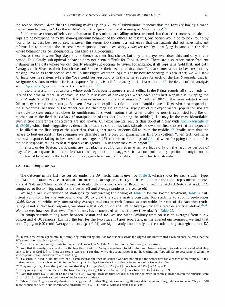
We begin our analysis by recalling Fig. 2b, which shows just how much gain over DA is possible if all subjects truth-tell, averaged across all possible preference and lottery draws. Of course, in the lab, it is possible that we get “bad draws” which undermine our potential to recreate the theoretical gains. To show that this is not the case, we construct a truth-telling counter factual, calculating the outcome distribution given the preference and lottery draws realized in the lab, but con-straining the truth-telling rate to be 100%. The CDF for this counter factual is in Fig. 3a. Fortunately, the gains are still quite large and are essentially identical to those that theory predicts: participants would have a 61.5% chance to receive their first choice under Boston, which is significantly larger than the 30.3% under DA with multiple lotteries (p < 0.01) and the 51.4% under DA with a single lottery (p < 0.01).51 When we compare the proportion of students who receive either their true first or second choice, once more Boston has significantly higher proportions than either DA or DA-SL (p < 0.01 in both cases).52

47 The 2% threshold was selected to give Table 5 a similar number of rows to Tables 2 and 4. The 10/15 was selected to give a bit more leeway for experimentation than the 4/5 threshold used in Tables 2 and 4. Results are not qualitatively different when different thresholds are used.48 This idea is not a new one; Pathak and Sönmez (2008) look at a model in which some player are optimally strategic and others sub-optimally truth-tell.49 It is not necessary to consider multiple versus single lottery setups under Boston: both yield the same distribution over outcomes.50 Tacitly, we are assuming that a different lottery structure won’t strongly affect the behavior of subjects. Ideally, we could check the robustness of this

assumption by look at the CDFs from just the first round, before subjects were exposed to feedback. Unfortunately, with only one round of data, those results are too noisy to be useful: Mann–Whitney tests fail to reject that there is even a difference across mechanisms in the fraction of subjects who get their first choice. Instead, we look at the CDFs for just the first five rounds of the uncorrelated treatment, where presumably feedback has not had as strong an effect as in later rounds. Doing this does not qualitatively change the results we discuss in the remainder of this section, but some differences only remain significant in one-sided Mann–Whitney tests.51 We use Mann–Whitney tests, where the session mean is a data point, that is, we have 7 data points for Boston, and 4 for DA and DA-SL. When we

only consider the last five periods, the p-values are 0.01 and less than 0.01, respectively.52 When we look at the last five rounds only, the difference between Boston and DA is still significant at p < 0.01, while the one between Boston and

DA-SL is not (p = 0.12).


Fig. 3. Outcome CDFs with preferences realized in lab (DA-SL is the single lottery counter-factual).

Now, we move to the actual outcome distribution observed in the lab. Even with a less than perfect truth-telling rate, we observe that a significantly larger fraction of students receive their true first choice with Boston than with DA (p < 0.01), or DA-SL (p = 0.06).53 When we compare the proportion of students who receive either their first or second choice, Boston once more significantly outperforms both DA (p < 0.01) and DA-SL (p = 0.09).54 These findings can be seen graphically in Fig. 3b.

Hence, it seems that the theoretical advantages of Boston over DA can indeed be realized in practice, at least in our specialized environment. This provides a proof-of-concept that non-strategy-proof mechanisms might perform well in the field if they are ordinal Bayes–Nash incentive-compatible.

5. Why did Boston succeed?

We have seen that Boston outperforms DA in the uncorrelated environment. In this section we provide some intuition for why this is the case by introducing a simple “art and science schools” example. We then extend the very simple

53 When we only consider the last five periods, Boston still gives a higher fraction of participants their first choice. The difference is significant when compared to DA (p < 0.01), though not when compared to DA-SL (p = 0.18). Note that a one-sided test would yield significance in all the two-sided tests that we have discussed.54 When we consider only the last five periods, the p values are < 0.01 and 0.03 respectively.


aaa aas ass sssasa sassaa ssa

S aa a S a aa SS as a S s as SS sa s S a sa SS ss s S s ss S

(a) The 8 (equally likely) states of the world from the ex ante perspective. Boxed cells indicate cells where Boston and DA give different overall matches.

(b) The 12 (equally likely) states of the world from the (interim) perspective of scientist S. Boxed cells indicate that Boston and DA give different schools to S.

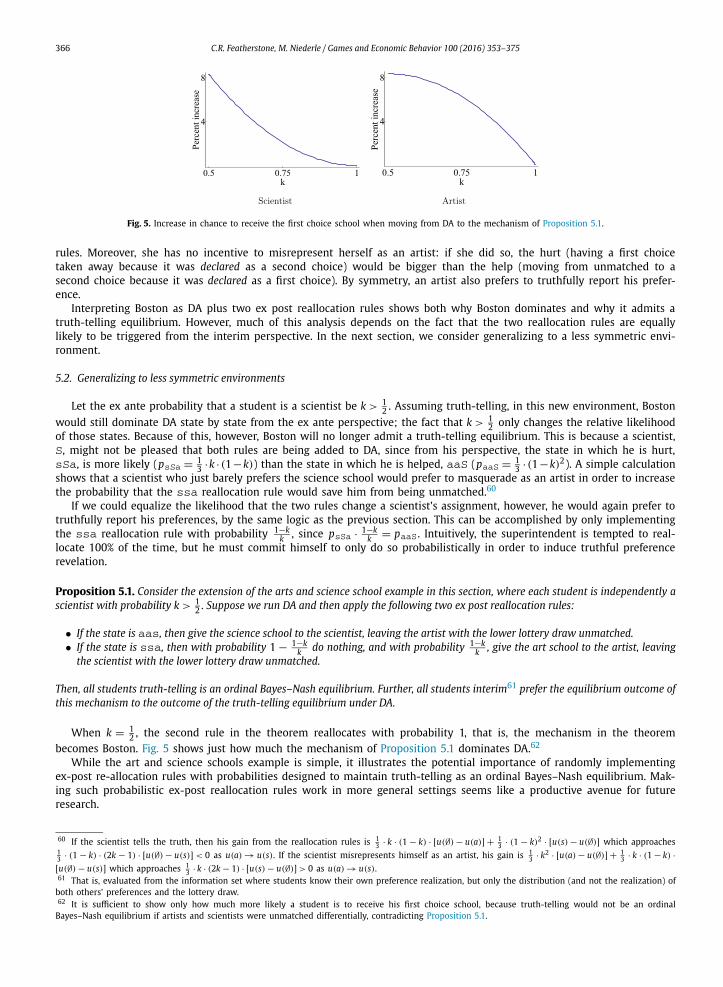
Fig. 4. States of the world: ex ante and interim.

example only slightly to show how to generate a mechanism that can handle some asymmetry which we might expect in many applications (and that is notably absent from the uncorrelated environment). The nature of this section is primarily to introduce an example for the sake of intuition; however, at the end, we will discuss where the example fits into the literature and how it sheds new light on non-strategy-proof market design.

5.1. The art and science schools example

Suppose there are three students and two one-seat schools – an art school and a science school. Each student is equally likely to be an artist (a) who prefers the art school or a scientist (s) who prefers the science school. All students find both schools acceptable, and a common lottery determines priorities at both schools. In this environment, similar logic to the proofs of Propositions 2.1 and 2.2 tell us that truth-telling is the unique equilibrium under both Boston and DA.

We will consider the outcomes of the two mechanisms both from the interim and ex ante points of view. States of the world from the ex ante perspective can be represented as a string containing three a’s or s’s; for instance, aas represents the state where the students with the highest two lottery draws are both artists, and the remaining student is a scientist.55

For interim states,56 we will use a capital letter to denote the student whose perspective we are considering; for instance,aaS represents the state of the world we just mentioned, from the perspective of the scientist with the lowest lottery draw.

The ex ante perspective is that of a social planner (the “superintendent”) who thinks about the quality of overall matches in terms of the distribution of how students rank their assigned schools.57 In this environment, such social preferences are equivalent to maximizing the probability that an agent gets his first choice.58 When comparing Boston and DA, the superintendent only cares about the two states in which the two mechanisms yield different matches: aas and ssa (see Fig. 4a). Intuitively, these are states where DA gives a school to a student who ranks it second, even though there is an unmatched student who ranked it first. Note that Boston never does this in any environment.59 So, assuming truth-telling, from the ex ante perspective, Boston is either the same as or better than DA in every state of the world. This is the precise way in which Boston outperforms DA.

Instead of Boston, however, consider running DA with the addition of a simple ex post reallocation rule: when the state of the world is aas, take the science school from the second artist and give it to the scientist. Assuming truth-telling, this clearly makes the superintendent better off, as it is the same as or better than DA in all states of the world. While ex ante students are better off, from the interim perspective the science student S is better off while an art student A is worse off. This may give an artist who is almost indifferent between the art school and the science school an incentive to masquerade as a scientist, since such an artist is more worried about being unmatched when the state is aas than about sometimes getting the science school instead of the art school. Analogously, we can also consider the “mirror image” of ouraas-contingent reallocation: an ssa-contingent rearrangement in which we take the art school from the second scientist and give it to the artist. By symmetry, this would make the superintendent and the artist better off, but would hurt the scientist and potentially give her incentive to misreport her preferences. It is not surprising that trying to improve upon DA ex post could cause incentive problems (Erdil and Ergin, 2008; Abdulkadiroglu et al., 2009; Featherstone, 2016). What is surprising in our example is that if we combine both of our problematic reallocation rules, we return to implementing truth-telling, although as an ordinal Bayes–Nash equilibrium instead of a dominant strategy equilibrium. In other words, Boston is equivalent to running DA and reallocating in the “bad” states of the world (aas and ssa).

To get a better look at why this works, consider the perspective of a scientist (capital-S) considering her preference report when both the aas and ssa reallocation rules are in effect. She cares most about the interim states sSa andaaS, as in those states, one of the reallocation rules changes the school she gets (see Fig. 4b). Although both sSa andaaS are equally likely from her perspective, the help she gets in aaS (moving from unmatched to a first choice) is bigger than the hurt she gets in sSa (moving from second choice to unmatched). So, she is interim better off under the new

55 Since we will only consider anonymous mechanisms, there is no need to keep track of whether the first artist is Student 1, 2, or 3. This simplifies the state space considerably without losing any of the intuition.56 That is, states from the perspective of a student who knows her own preferences, but not those of others and not the lottery draw.57 This is a common and natural way to aggregate welfare with limited information. See Featherstone (2016) for more.58 Everyone is unmatched one-third of the time by symmetry, so the ex ante probability of getting a first choice is sufficient for the entire distribution of

ranks received.59 Kojima and Ünver (2013) show that Boston “respects preference rankings”, which implies the statement above. Intuitively, this is because, under Boston,

if a student is rejected by his kth ranked school, it must have filled up by being assigned students who ranked it kth or higher.


Fig. 5. Increase in chance to receive the first choice school when moving from DA to the mechanism of Proposition 5.1.

rules. Moreover, she has no incentive to misrepresent herself as an artist: if she did so, the hurt (having a first choice taken away because it was declared as a second choice) would be bigger than the help (moving from unmatched to a second choice because it was declared as a first choice). By symmetry, an artist also prefers to truthfully report his prefer-ence.

Interpreting Boston as DA plus two ex post reallocation rules shows both why Boston dominates and why it admits a truth-telling equilibrium. However, much of this analysis depends on the fact that the two reallocation rules are equally likely to be triggered from the interim perspective. In the next section, we consider generalizing to a less symmetric envi-ronment.

5.2. Generalizing to less symmetric environments

Let the ex ante probability that a student is a scientist be k > 12 . Assuming truth-telling, in this new environment, Boston

would still dominate DA state by state from the ex ante perspective; the fact that k > 12 only changes the relative likelihood

of those states. Because of this, however, Boston will no longer admit a truth-telling equilibrium. This is because a scientist,S, might not be pleased that both rules are being added to DA, since from his perspective, the state in which he is hurt,sSa, is more likely (psSa = 1

3 ·k · (1 −k)) than the state in which he is helped, aaS (paaS = 13 · (1 −k)2). A simple calculation

shows that a scientist who just barely prefers the science school would prefer to masquerade as an artist in order to increase the probability that the ssa reallocation rule would save him from being unmatched.60

If we could equalize the likelihood that the two rules change a scientist’s assignment, however, he would again prefer to truthfully report his preferences, by the same logic as the previous section. This can be accomplished by only implementing the ssa reallocation rule with probability 1−k

k , since psSa · 1−kk = paaS . Intuitively, the superintendent is tempted to real-

locate 100% of the time, but he must commit himself to only do so probabilistically in order to induce truthful preference revelation.

Proposition 5.1. Consider the extension of the arts and science school example in this section, where each student is independently a scientist with probability k > 1

2 . Suppose we run DA and then apply the following two ex post reallocation rules:

• If the state is aas, then give the science school to the scientist, leaving the artist with the lower lottery draw unmatched.• If the state is ssa, then with probability 1 − 1−k

k do nothing, and with probability 1−kk , give the art school to the artist, leaving

the scientist with the lower lottery draw unmatched.

Then, all students truth-telling is an ordinal Bayes–Nash equilibrium. Further, all students interim61 prefer the equilibrium outcome of this mechanism to the outcome of the truth-telling equilibrium under DA.

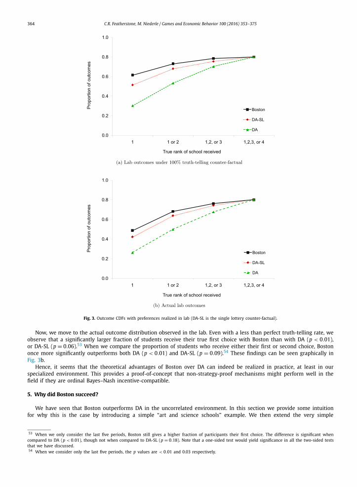
When k = 12 , the second rule in the theorem reallocates with probability 1, that is, the mechanism in the theorem

becomes Boston. Fig. 5 shows just how much the mechanism of Proposition 5.1 dominates DA.62

While the art and science schools example is simple, it illustrates the potential importance of randomly implementing ex-post re-allocation rules with probabilities designed to maintain truth-telling as an ordinal Bayes–Nash equilibrium. Mak-ing such probabilistic ex-post reallocation rules work in more general settings seems like a productive avenue for future research.

60 If the scientist tells the truth, then his gain from the reallocation rules is 13 · k · (1 − k) · [u(∅) − u(a)] + 1

3 · (1 − k)2 · [u(s) − u(∅)] which approaches 13 · (1 − k) · (2k − 1) · [u(∅) − u(s)] < 0 as u(a) → u(s). If the scientist misrepresents himself as an artist, his gain is 1

3 · k2 · [u(a) − u(∅)] + 13 · k · (1 − k) ·

[u(∅) − u(s)] which approaches 13 · k · (2k − 1) · [u(s) − u(∅)] > 0 as u(a) → u(s).

61 That is, evaluated from the information set where students know their own preference realization, but only the distribution (and not the realization) of both others’ preferences and the lottery draw.62 It is sufficient to show only how much more likely a student is to receive his first choice school, because truth-telling would not be an ordinal

Bayes–Nash equilibrium if artists and scientists were unmatched differentially, contradicting Proposition 5.1.


5.3. Comparison to the existing literature

In the broader school choice literature, models tend to hinge on the assumption of complete information, evaluating efficiency from the concomitant ex post perspective. The model in this paper adds to an important, but relatively sparse,branch of the school choice literature that considers incomplete information and interim Pareto efficiency (see e.g. Ergin and Sönmez, 2006; Erdil and Ergin, 2008; Abdulkadiroglu et al., 2011, and Troyan, 2012). Even among this small literature, our theoretical approach is further distinguished by looking at truth-telling equilibria of non-strategy-proof mechanisms. Finally, we also limit ourselves to equilibria and efficiency claims that are ordinal in nature, that is, they hold regardless of the cardinal preferences that underlie the ordinal preferences.

Perhaps it is easiest to see the distinctions by comparing our model to the model that we think of as the closest com-plement to our own, Abdulkadiroglu et al. (2011). Their paper presents a simple model in which all agents have the same ordinal preferences, but different underlying cardinal preferences. In this incomplete information setting, they show that all agents prefer the outcome of any equilibrium of the Boston mechanism to the outcome of the truth-telling equilibrium of DA. As in our paper, this claim is made from the interim perspective in which agents know their preferences, but not those of the other agents. Their claim depends on agents submitting a generically non-truthful report, and requires agents to have correct beliefs about the distribution of cardinal preferences in the market and to best respond to those beliefs. In contrast, our simple model requires the market designer to calibrate the correct mechanism in order to implement truth-telling as an ordinal Bayes–Nash equilibrium, freeing participants from performing any calculations when submitting their preferences.

We think of both models as being simple demonstrations of the feasibility of two approaches for non-strategy-proof market design. In one agents must best-respond to fine grained cardinal information, while in the other, it must be safe to submit preferences truthfully for any cardinal information that could rationalize the ordinal information. Our approach assumes less of the agents, but requires more of the market designer, due to the constraint given by requiring truth-telling. Furthermore, the gains from our approach come from relatively uncorrelated preferences, while the gains of the other approach are generated by aligned preferences.

6. Conclusion

We had two goals for our experiment. The first concerns the new and active literature on mechanisms that rely on equilibrium manipulation of preference reports to implement outcomes superior to those of DA (Miralles, 2009; Troyan, 2012; Abdulkadiroglu et al., 2015). To assess the viability of these approaches for practical market design, it is important to determine whether participants are likely to at least come close to equilibrium play. Empirical work suggests that this may not be the case for at least a few participants (Abdulkadiroglu et al., 2005b). Existing experiments have focused on whether participants submit preferences truthfully in non-strategy-proof mechanisms, and while these papers confirm that participants would manipulate their preferences, they in general do not provide participants with sufficient information to calculate the equilibrium (Chen and Sönmez, 2006; Pais and Pintér, 2008; Calsamiglia et al., 2010).

The first result of the present paper is that non-truth-telling equilibria might be hard to implement. In the aligned preference environment, while DA elicited truth-telling, Boston elicited sub-optimal manipulation of preference reports. This was the case even in the last five periods of play, where participants had ample experience and received precise feedback in a very simple environment. This leaves two potential ways to move the “improving on strategy-proof mechanisms” literature forward. The first is to give serious thought to how students can be pushed in the direction of equilibrium. Inquiry into this question seems like a fruitful and understudied line of experimental research, but is not what we pursue in this paper. The second is to weaken the implementation of the truth-telling equilibrium.

The second part of our paper shows that truth-telling equilibria that are not implemented in dominant strategies do have the potential to succeed, both in inducing truthful reporting and in yielding efficiency gains. We think of our results as showing that there is potential for the incentive-compatible-but-not-strategy-proof research agenda to succeed. Further theoretical development is clearly required, but, as we hope our experiment has demonstrated, such a research agenda could potentially have a large impact on student welfare.

In addition to simply pointing out that Boston can dominate DA in some environments, we have also tacitly made two suggestions for non-strategy-proof design. The first is to implement truth-telling as an ordinal Bayes–Nash equilibrium, as it requires information about the distribution of ordinal preferences (which can be observed under a strategy-proof mechanism), but not about the cardinal preferences, which are more elusive.63 The second is to analyze efficiency and incentives from the interim information set, in which a student knows his own preferences, but only the distribution of others’. Not only does this seem like the natural assumption for what real-world students know, but from an efficiency standpoint, it seems like the sort of “best outcome averaged over many years” sort of calculus that seems natural for a school board.

63 For instance, in any school district currently running a strategy-proof mechanism, we have good reason to believe that submitted ordinal preferences are truthful. From these, we can construct a model of the distribution from which the ordinal preferences came. Note that these preference reports contain no information about the underlying cardinal preferences (except that they should rationalize the submitted ordinal preferences). Such a model of the distribution of preferences could inform a design for subsequent years that implements truth-telling only via an ordinal Bayes–Nash equilibrium.


Table A.6Unambiguously sub-optimal behavior of Top students.

Best response for Top students (BR)

# sessions where BR is weakly optimal in each of the last 5 rounds (fraction of rounds where the BR is strict)

Fraction of Tops who truth-tell at least 4 of the last 5 rounds

Fraction of Tops who BR in at least 4 of the last 5 rounds

Skip the middle 2 (4/5) 5/6 0/6Skip the middle 2 (3/5) 2/6 2/6Don’t skip the middle 1 (4/5) 3/3 3/3

Appendix A. Best-response analysis for aligned environment under Boston

There are two cases present in the data which give Top students strict incentives to rank either Silver or Bronze as their second choice, given that they ranked Gold as their first choice.

Case 1 (Skip the middle): All Top students rank Gold as their first choice, at least one Average ranks Silver as his first choice, and one of the Averages who is not assigned in the first round ranks Bronze as his second choice. Tops are then constrained to rank Bronze as their second choice. Here, the expected payoff difference between ranking Silver second or Bronze second is 1

3 · 25 = 8 13 , which is 11% of the best-response payoff of 100 · 2

3 + 25 · 13 = 75.

Case 2 (Do not skip the middle): All Top students rank Gold as their first choice, at least one Average ranks Bronze as his first choice, and one of the Averages who is not assigned in the first round ranks Silver as his second choice. Tops are then constrained to rank Silver second. Here, the expected payoff difference between ranking Silver second or Bronze second is 1

3 · 67 = 22 13 , which is 25% of the best-response payoff of 100 · 2

3 + 67 · 13 = 89.

We restrict ourselves to studying sessions in which a large fraction (4 out of 5) or at least the majority (3 out of 5) of the last 5 periods are either in Case 1 or Case 2 and in which the remaining of the last five periods do not fall into any of these two cases. That is, we focus on sessions in which Top students weakly best respond by submitting (Gold, Silver, x)or (Gold, Bronze, x) in all five last periods, and, in 4 (or 3) of those periods, this behavior is a strict best response. The columns of Table A.6 show the number of sessions that fall into these categories, what fraction of the Top students submit truthfully (i.e. submit (Gold, Silver, x)) as a primary strategy, that is 4 out of 5 times, and what fraction of the Top students best respond as a primary strategy. Note that Table A.6 analyzes 4 distinct “Skip the middle” sessions.

Appendix B. Proofs

B.1. The model

Let there be a finite set of students, I , and a finite set of schools, S . Also, let ∅ /∈ S represent the outcome of being unmatched. Each student i has a strict preference Pi over the elements of S ∪ {∅}, and each school s has a strict priority ordering �s over I .64 Denote the number of acceptable schools in a preference Pi by |Pi | ≡ |{s ∈ S : s P i ∅}|. As we are dealing with individually rational mechanisms, we will only consider the ordering of schools in Pi that are ranked above ∅, that is, if two preferences order their acceptable schools in the same way, then they are considered the same preference. A utility function ui rationalizes a preference Pi if ui(Pi(a)) > ui(Pi(b)) ⇔ a Pi b, where Pi(a) denotes the ath ranked school in Pi . q ≡ (qs)s∈S is a vector of capacities for each school. The unmatched outcome, ∅, can be thought of as a special “school” with q∅ = ∞. P ≡ (Pi)i∈I and �≡ (�s)s∈S are drawn from a joint probability distribution λ (P ,�).

A school choice problem is defined by 〈I,S,q, λ〉. A matching μ : I → S ∪ {∅} is a function such that |{i : μ(i) = s}| ≤ qs

for all s ∈ S . A deterministic mechanism is a function ϕ that maps reported student preferences P and school priorities �to a matching. Let ϕi

(P ;�)

be shorthand for ϕ(

P ;�)(i). For a student, a strategy in the Bayesian game induced by a

school choice problem and a deterministic mechanism is a mapping from true preferences to reported preferences, σi ; let σ ≡ (σi)i∈I denote a strategy profile. A strategy profile is a Bayes–Nash equilibrium if no student has a profitable unilateral deviation, that is, ∀i, Pi, Pi

E {ui [ϕi (σ (P ) ;�)]|Pi} ≥ E{

ui[ϕi

(P i,σ−i (P−i) ;�)]∣∣Pi

}.

A set of strategies is an ordinal Bayes–Nash equilibrium if a student does weakly worse (in the first-order stochastic sense) when he deviates from equilibrium, that is, ∀i, Pi, Pi, |Pi | ≥ b ≥ 1

b∑a=1

Pr {ϕi (σ (P ) ;�) = Pi (a)|Pi} ≥b∑

a=1

Pr{ϕi

(P i,σ−i (P−i) ;�) = Pi (a)

∣∣Pi}.

64 Note that �s is not an ordering over I ∪ {∅}, that is, schools are required to find all students acceptable.


B.2. The aligned environment

Proof of Proposition 2.1. Recall that truth-telling is a weakly dominant strategy for the proposing side in two-sided DA. For our one-sided setting, this means that truth-telling does at least as well as any other strategy ex post, that is, after other students’ preferences and the lottery draws are known. Hence, if we can show one lottery draw that occurs with positive probability, where truth-telling is strictly better for some student i than some alternative strategy P i , regardless of the other students’ submitted preferences, then we have shown that P i is strictly dominated by truth-telling for i. Using this approach, we apply iterated deletion of strictly dominated strategies (IDOSDS).

Round 1: Delete any strategies played by Tops that fail to rank Gold first. This is valid because a Top is ranked first by all schools with positive probability. When this happens, ranking Gold first is strictly better than ranking anything else first.

Round 2: Delete any strategies played by Tops that fail to rank Gold first and Silver second. This is valid because a Top is ranked third by all schools with positive probability. With the strategies that remain, the Tops who are ranked first and second at Gold will get Gold, and our third-ranked Top will get whatever he ranks second. Ranking Silver second is strictly better than anything else that remains.

Round 3: Delete any strategies played by Averages that fail to report Bronze acceptable. This is valid because an Average is ranked fourth by all schools with positive probability. With the strategies that remain after Round 2, the Tops will take Gold and Silver, leaving one seat at Bronze. If our fourth-ranked Average reports Bronze acceptable, he gets it, which is strictly better than going unmatched, which is what would happen if he failed to report Bronze acceptable.

So far, IDOSDS has left us with the family of strategy profiles in the statement of the proposition. As IDOSDS cannot remove strategies used in equilibrium, any equilibrium profile must be in our family. Now, we show that all profiles in the family are equilibria. First, note that relative to any of these profiles, any stable match must give Gold to the two Tops with the best lottery draw at Gold, Silver to the other Top, and Bronze to the Average with the best lottery draw at Bronze. The remaining Average is unmatched, which gives us the outcome equivalence result in the statement of the proposition. As the lottery is fair and independent of reported preferences, any profile in our family will lead to a Top getting Gold 2

3 of the time and Silver 1

3 of the time, and an Average getting Bronze half the time and remaining unmatched the other half of the time. Hence, all students are equally well off in any of the profiles of our family, which shows that all profiles in the family of profiles that survive IDOSDS are equilibria. �Proof of Proposition 2.2. We begin by showing that all three Tops must rank Gold first in equilibrium. We do so by ruling out the other possibilities. First, by way of contradiction, assume an equilibrium where two or more Tops fail to rank Gold first. Of those Tops, one must not be getting Gold 100% of the time. If this Top were to rank Gold first, he would get Gold 100% of the time, which would be a profitable deviation, a contradiction.

Now, by way of contradiction, assume an equilibrium in which exactly two Tops rank Gold first. The Top who doesn’t rank Gold first will get whatever else he ranks first; hence, he must rank Silver first. Given these rankings from the Tops, the Averages can only get Bronze or remain unassigned. In equilibrium, they must both rank Bronze first. To see this, consider the following two cases. If exactly one Average were ranking Bronze first, then the other Average could profitably deviate by ranking Bronze first as well. If no Averages rank Bronze first, then one of them who isn’t getting Bronze 100% of the time could do so by ranking Bronze first, a profitable deviation. Hence, we have two Tops ranking Gold first, one Top ranking Silver first, and both Averages ranking Bronze first. But in this scenario, the Top who ranks Silver first can profitably deviate by ranking Gold first and Silver second, since Silver will still remain for him in round two of the Boston algorithm. This is a contradiction of our initial hypothesis.

So, we have shown that there must be three Tops ranking Gold first in any pure-strategy equilibrium. This means that both Averages must rank Silver first in equilibrium. To see this, we assume otherwise and check the cases. If neither Average ranks Silver first, then one of them must not be getting Silver 100% of the time. But that Average could guarantee himself Silver by ranking Silver first, a contradiction. If exactly one Average ranks Silver first, then the other Average is getting a payoff of 25 (from Bronze) at best. But by ranking Silver first, that Average could guarantee himself a payoff of at least 12 · 67 = 33.5 > 25, a contradiction (recall that the statement of the theorem assumes that agents are risk-neutral).

So, we have shown that in any pure-strategy equilibrium, all Tops rank Gold first, and both Averages rank Silver first. This means Gold and Silver will be filled in the first round of the Boston algorithm, leaving one Top and one Average behind to vie for the seat at Bronze in the second round. In equilibrium, the Average cannot get the seat, as if he did, the Top could profitably deviate by ranking Bronze second. Moreover, in equilibrium, the Top must get Bronze in the second round of the algorithm, as if he didn’t, the Average could guarantee himself the seat by ranking Bronze second, contradicting what we have already shown (that the Average cannot get the seat at Bronze in equilibrium). And since all Tops have a 1

3 chance of being the Top in the second round of the algorithm, they must all rank Bronze second.

Hence, in any pure-strategy equilibrium, all Tops rank Gold first and Bronze second, and all Averages rank Silver first, demonstrating the “only if” part of the proposition. For the “if” part, it is easy to check that in any profile of strategies


that meets our conditions, there is no profitable unilateral deviation for any player. Finally, note that the conditions pin down the outcome of the match: two Tops get Gold, one Top gets Bronze, one Average gets Silver, and one Average goes unmatched. �B.3. The uncorrelated environment

We begin our analysis of the uncorrelated environment by looking at DA. Under DA, there is always a truth-telling ordinal Bayes–Nash equilibrium.

Lemma B.1. Under DA, for any school choice problem, there exists an ordinal Bayes–Nash equilibrium where all students are truth-telling.

Proof. Since truth-telling is weakly dominant for the proposing side in two-sided DA, we know that in our one-sided DA setup, by reporting truthfully, a student guarantees himself a weakly better assignment for every realization of reported preferences and priorities,

(P−i;�

). This state-by-state weak dominance of truth-telling is sufficient for truth-telling to

yield a distribution over outcomes that weakly first-order stochastically dominates any other response to any profile of other students’ strategies. Hence, all students truth-telling is an ordinal Bayes–Nash equilibrium. �

In the uncorrelated environment, this equilibrium is unique.

Lemma B.2. The revelation game induced by DA in the uncorrelated environment is dominance solvable.

Proof. To show that truth-telling is the unique Bayes–Nash equilibrium, we will implement the same strategy from the proof of Proposition 2.1, using the following rounds of iterated deletion of strictly dominated strategies (IDOSDS):

Round 1: Delete all strategies that don’t report rank 1 truthfully. If a student who failed to do so were ranked first at all schools, which occurs with positive probability, then he would do strictly better to tell the truth.

Round 2: Delete all strategies that don’t report ranks 1 and 2 truthfully. If all students share the same preference, and one of them were ranked second at all schools, then that student would do strictly better to report rank 2 truthfully (as he will not get his truthfully reported rank 1 school). This event occurs with positive probability.

...

The logical end of this progression is that all strategies except for truth-telling are deleted. In other words, the revelation game induced by DA in the uncorrelated environment is dominance solvable. �

These two lemmas establish Proposition 2.3 from the main text.

Proof of Proposition 2.3. Lemma B.1 establishes that all students truth-telling is an ordinal Bayes–Nash equilibrium, and Lemma B.2 established uniqueness, since dominance solvable games have a unique equilibrium. �

Now, we move onto the behavior of Boston in the uncorrelated environment. We will focus on school choice problems that have a certain symmetry property. Let P s↔s′

i denote the alteration of Student i’s preferences in which the positions of schools s and s′ are switched. Similarly, let P s↔s′ denote the same alteration applied to the complete profile of students, and let P s↔s′

−i denote the same alteration applied to the profile of preferences of all students except for Student i. Finally, let �s↔s′ be the vector of schools’ orderings where the orderings of schools s′ and s are switched.

Definition B.1. A probability distribution λ is school-symmetric with respect to i if λ [(P ; �)|Pi] = λ [(

Pi, P s↔s′−i ; �s↔s′

)∣∣∣Pi

]for all s, s′ ∈ S whenever the equation is defined.65 A school choice problem is school-symmetric with respect to i if its distribution is school-symmetric and qs = qs′ , ∀s, s′ ∈ S . We simply call a distribution or school-choice problem school-symmetric if it is school-symmetric with respect to i for all i ∈ I .

This definition does not allow for interchanges that involve ∅, as ∅ /∈ S . Also, note that school-symmetry is not the same as drawing preferences from the uniform distribution; for instance, it allows for a student to believe that other students are more likely to find five schools acceptable than two. With school-symmetric reported preferences, we can show that

65 For instance, if the probability of some Pi were zero, the equation would be undefined, since conditioning on a probability zero event is undefined.


truth-telling does at least as well as any other strategy a student might play. We do this via two lemmas. Let Bi [P ;�]denote student i’s assignment under Boston when the reported preferences are P and the school priorities are �.

Lemma B.3. Let s′ Pi s. Then,

a) If neither Pi or P s′↔si get s or s′ for i when he reports them, then he gets the same school when reporting either preference, that is,

Bi

[P s′↔s

i , P−i; �]

/∈ {s′, s

}and Bi [P ; �] /∈ {

s′, s}

⇒ Bi

[P s′↔s

i , P−i ; �]

= Bi [P ; �] .

b) If i fails to get s′ under Pi , then he will also fail to get it under P s′↔si , that is,

Bi[P ; �] �= s′ ⇒ Bi[P s′↔si , P−i ; �] �= s′.

c) If i gets s under Pi , then he also gets it under P s′↔si , that is,

Bi[P ; �] = s ⇒ Bi[P s′↔si , P−i ; �] = s.

d) Being truthful about whether a school is acceptable never makes i worse off.

Proof. Recall that what the Boston algorithm does in a given round depends solely on who isn’t matched yet and which seats are left. Let r′ , r, and rB be the ranks of s′ , s, and Bi [P ;�], respectively, that is, let Pi(r′) = s′ , Pi(r) = s, and Pi

(rB

) =Bi [P ; �].

a) By assumption, rB �= r′ . If rB < r′ , then i must also be assigned in round rB when he reports P s′↔si , as switching s and s′

won’t change what seats and students are still available at the start of round rB . If rB > r′ , then by our assumptions that Bi

[P s′↔s

i , P−i; �]

/∈ {s′, s

}and Bi [P ; �] /∈ {

s′, s}

, the seats at both s and s′ must be exhausted at the end of round r′ . Hence, the set of students and seats that remain available is the same for both reports going forward from round r′ . So i is assigned in round rB under both preference reports.

b) Since i is rejected in round r′ when he reports Pi , there must not be any seats available at s′ at the end of round r′ . Since he didn’t take a seat at s′ when he reported Pi , there must also not be any seats available at the end of round r′when he reports P s′↔s

i . Hence he cannot get s′ by ranking it r > r′ .c) Pi and P s′↔s

i are identical down to rank r′ − 1, so i must be unmatched at the start of round r′ , since he isn’t matched until round r > r′ when he reports Pi . This also tells us that there must be at least one unclaimed seat at s at the end of round r′ when i reports Pi . Reporting P s′↔s

i allows i to get this seat.d) If i fails to report a truly acceptable school s′′ acceptable, ranking it between the lowest ranked acceptable school

and ∅ in the original report either does not affect what i gets, or allows i to get s′′ instead of ∅. Now, consider the lowest unacceptable school s′′′ that i reports acceptable. Reporting s′′′ unacceptable and moving all schools originally declared inferior to s′′′ up one position in the reported rank order either does not affect what i gets or allows him to get something he prefers to s′′′ instead of s′′′ . �

Lemma B.4. Under the Boston mechanism, if the distribution of submitted preferences and school priorities is school-symmetric with respect to i and qs = qs′ , ∀s, s′ ∈ S , then for i, truth-telling weakly first-order stochastically dominates any other preference report.

Proof. Note that the proof of this theorem borrows heavily from the methods of Roth and Rothblum (1999). To start, Part d) of Lemma B.3 tells us that there is no loss in limiting ourselves to reports that declare a school acceptable if and only if it is truly acceptable. Now, consider a student, i, who truthfully prefers school s′ to s, that is s′ Pi s. Table B.7a lists the possibilities for what i gets with and without switching s and s′ . Parts b) and c) of Lemma B.3 rule out the cells labeled “Impossible”, while Part a) tells us that u must be the same for both Truth and Lie in Case A.

Now, for each of the cases in Table B.7a, we can write out what i gets when he tells the truth and what he gets when he swaps s and s′ . These are the first and third columns of Table B.7b. Looking at just these columns, however, it is not clear that i doesn’t want to tell the lie: in Cases B and D, it could potentially make him better off. To show that he does better with the truth, note that Boston is label-independent, that is, if we merely change the names of two schools with the same capacity, then the output of Boston will be the same, modulo the name change. Mathematically, if qs = qs′ , then

Bi [P ;�] = u /∈ {s′, s

} ⇔ Bi

[P s′↔s;�s′↔s

]= u,

Bi [P ;�] = s′ ⇔ Bi

[P s′↔s;�s′↔s

]= s,

Bi [P ;�] = s ⇔ Bi

[P s′↔s;�s′↔s

]= s′.


Table B.7Cases and outcomes for Lemma B.4.

(a) Table of cases

Lie: Bi [P s′↔si , P−i ; �]

= u /∈ {s, s′} = s = s′

Truth: Bi [Pi , P−i ; �] = u /∈ {s, s′} Case A Case B Impossible= s Impossible Case C Impossible= s′ Case D Case E Case F

(b) Outcomes for the cases

Truth Lie (swap s and s′)Bi [Pi , P−i;�] Bi [Pi , P s′↔s

−i ;�s′↔s] Bi [P s′↔si , P−i;�] Bi [P s′↔s

i , P s′↔s−i ;�s′↔s]

Case A u u u uCase B u s′ s uCase C s s′ s s′Case D s′ u u sCase E s′ s′ s sCase F s′ s s′ s

This allows us to use the first column of Table B.7b to fill in the fourth, and the third to fill in the second. Now, by school-symmetry, the two columns under Truth in Table B.7b are equally likely if i truthfully orders s and s′ , and the two columns under Lie are equally likely if i reverses their ordering. Row by row, truthfully ordering s and s′ is at least as good as, and sometimes better than, switching their ordering. In other words, we can partition the states-of-the-world in such a way that, for each element of the partition, ordering s and s′ truthfully weakly first-order stochastically dominates reversing their order. This implies that truthfully ordering s and s′ weakly first-order stochastically dominates any other report. Hence, truth-telling weakly first-order stochastically dominates any other strategy. �

We have thus established conditions under which Boston admits a truth-telling equilibrium.

Proposition B.1. Under the Boston mechanism, if a school choice problem is school-symmetric, then there exists an ordinal Bayes–Nash equilibrium where all students are truth-telling.

Proof. If all students but i are truth-telling, then their reports are school-symmetric with respect to i. By Lemma B.4, truth-telling weakly first-order stochastically dominates any other strategy for i. Hence, all students truth-telling is an ordinal Bayes–Nash equilibrium. �

To get uniqueness, we will need to restrict ourselves to a class of strategies that is natural for symmetric environments.

Definition B.2. A strategy σi is anonymous if for any s, s′ ∈ S and for any Pi , σi

(P s′↔s

i

)= (σi (Pi))

s′↔s .

Anonymous strategies are useful to us because they translate school-symmetric true preferences into school-symmetric reported preferences, allowing us to leverage Lemma B.4.

Lemma B.5. If the distribution of true preferences and school priorities is school-symmetric with respect to i, then when all students besides i ∈ I play anonymous strategies, the distribution of students’ reported preferences and school orderings is school-symmetric with respect to i.

Proof. The strategies used by the students induce a distribution over reported preferences and school priorities:

λσ (P−i;� |Pi) ≡∑

{�−i : σ−i

(�−i

)=P−i}λ(�−i;� |Pi) .

Using this definition, we get

λσ

(P s′↔s

−i ;�s′↔s |Pi

)=

∑{�−i : σ−i

(�−i

)=P s′↔s−i

}λ(�−i;�s′↔s |Pi

)

=∑

{�−i : σ−i

(�s′↔s

−i

)=P s′↔s

−i

}λ(�s′↔s

−i ;�s′↔s |Pi

)


=∑

{�−i : (σ−i

(�−i

))s′↔s=P s′↔s−i

}λ (�−i;� |Pi)

=∑

{�−i : (σ−i

(�−i

))=P−i}λ(�−i;� |Pi)

= λσ (P−i;� |Pi) ,

where the second equality comes from re-indexing the sum, the third comes from the definitions of anonymous strategies and school-symmetric distributions, the fourth comes from applying the s′ ↔ s operator to both sides of the condition in the index set, and the final inequality comes from the definition of λ. So, the distribution of students’ reported preferences and school orderings is school-symmetric with respect to i. �

Now, we are in a position to prove the uniqueness of the truth-telling equilibrium under Boston in the uncorrelated environment.

Proof of Proposition 2.4. By Proposition B.1, we know that truth-telling is an ordinal Bayes–Nash equilibrium. Now, we show it is the unique such equilibrium in anonymous strategies. Assume an equilibrium in anonymous strategies. By Lemmas B.4and B.5, a student i in such an equilibrium can’t be hurt by switching to truth-telling. We will now proceed by ruling out strategies that can’t be used in such an equilibrium.

Round 1a: Delete all strategies that fail to report some school acceptable. If student i is the top-priority student at his first choice school, then he does strictly better to rank it first.

Round 1b: Delete all strategies that don’t truthfully report the first choice school. Say that i falsely reports his first choice school. Since students are playing anonymous strategies and ranking at least one school, it is possible that all students rank the same school first, and that i is the top priority student at that school. Falsely reporting his first choice school is strictly worse than truthfully reporting.

Round 2a: Delete all strategies that fail to report two schools acceptable. Say that all students share i’s preference and he has second priority at his second choice school. Failing to report that school acceptable is strictly worse than truth-telling.

Round 2b: Delete all strategies that don’t truthfully report the second choice school. Say that i falsely reports his second choice school. Since students are playing anonymous strategies and ranking at least two schools, it is possible that all students rank the same schools first and second, and that i is the second priority student at his true second choice. Falsely reporting his second choice is strictly worse than truthfully reporting.

...

The logical end of this process is to eliminate all strategies except for truth-telling. Hence, the truth-telling equilibrium is the unique Bayes–Nash equilibrium in anonymous strategies for the revelation game induced by Boston in the uncorrelated environment. �B.4. The arts and science schools example

Proof of Proposition 5.1. Assume that agent i is a scientist and that all agents besides i are truth-telling. Let π Zi (x | Y ) de-

note the probability that agent i gets school x ∈ {a, s,∅} under mechanism Z ∈ {D A, New} (where “New” is the mechanism described in the statement of the proposition) when he declares himself of type Y ∈ {S, A} (where S and A represent sci-entist and artist, respectively). By the strategy-proofness of DA, we know that for i, truth-telling ordinally dominates other strategies, that is,66

π D Ai (s | S) ≥ π D A

i (s | A), (B.1)

π D Ai (∅ | S) ≤ π D A

i (∅ | A).

Now, since the “New” mechanism introduced in the statement of the proposition is simply DA followed by an ex-post rearrangement rule, we can easily derive similar probabilities under it:

π Newi (s | S) = π D A

i (s | S) + paaS

π Newi (s | A) = π D A

i (s | A) − paAs,

66 Note that the second inequality is equivalent to π D Ai (s | S) + π D A

i (a | S) ≥ π D Ai (s | A) + π D A

i (a | A), since π D Ai (s | S) + π D A

i (a | S) + π D Ai (∅ | S) =

π D Ai (s | S) + π D A

i (a | A) + π D Ai (∅ | A) = 1.


π Newi (∅ | S) = π D A

i (∅ | S) − paaS + 1 − k

k· psSa,

π Newi (∅ | A) = π D A

i (∅ | A) + paAs − 1 − k

k· pssA.

Plugging in paaS = 13 · (1 − k)2, pssA = 1

3 · k2, and paAs = psSa = 13 · k · (1 − k), these probabilities reduce to

π Newi (s | S) = π D A

i (s | S) + 1

3· (1 − k)2 ,

π Newi (s | A) = π D A

i (s | A) − 1

3· k · (1 − k) ,


i (∅ | S),


i (∅ | A).

Clearly these probabilities meet the ordinal Bayes–Nash equilibrium inequalities (Eq. B.1), just like the DA probabilities67; so, for the scientist, truth-telling is an ordinal best-response to other agents truth-telling. An almost identical line of reasoning shows the same thing for the artist.68 This establishes that truth-telling is an ordinal Bayes–Nash equilibrium under the “New” mechanism.

Further, since π Newi (s | S) > π D A

i (s | S) and π Newi (∅ | A) = π D A

i (∅ | A), it is also true that the scientist interim ordinally prefers his outcome under the “New” truth-telling equilibrium to his outcome under the DA truth-telling equilibrium. Again, an almost identical line of reasoning shows the same thing for the artist.69 Hence, all agents interim ordinally prefer the truth-telling equilibrium outcome under the “New” mechanism to the truth-telling equilibrium outcome under DA. �References

Abdulkadiroglu, A., Che, Y.-K., Yasuda, Y., 2015. Expanding “choice” in school choice. Am. Econ. J. Microecon. 7 (1), 1–42.Abdulkadiroglu, A., Che, Y.-K., Yasuda, Y., 2011. Resolving conflicting preferences in school choice: the “Boston” mechanism reconsidered. Amer. Econ.

Rev. 101 (1), 399–410.Abdulkadiroglu, A., Pathak, P.A., Roth, A.E., 2005a. The New York city high school match. Amer. Econ. Rev. 95 (2), 364–367.Abdulkadiroglu, A., Pathak, P.A., Roth, A.E., 2009. Strategy-proofness versus efficiency in matching with indifferences: redesigning the NYC high school

match. Amer. Econ. Rev. 99 (5), 1954–1978.Abdulkadiroglu, A., Pathak, P.A., Roth, A.E., Sönmez, T., 2005b. The Boston public school match. Amer. Econ. Rev. 95 (2), 368–371.Abdulkadiroglu, A., Pathak, P.A., Roth, A.E., Sönmez, T., 2006. Changing the Boston school choice mechanism. Working paper.Abdulkadiroglu, A., Sönmez, T., 2003. School choice: a mechanism design approach. Amer. Econ. Rev. 93 (3), 729–747.Barberà, S., Dutta, B., 1995. Protective behavior in matching models. Games Econ. Behav. 8 (2), 281–296.Budish, E., Cantillon, E., 2012. The multi-unit assignment problem: theory and evidence from course allocation at Harvard. Amer. Econ. Rev. 102 (5),

2237–2271.Calsamiglia, C., Haeringer, G., Klijn, F., 2010. Constrained school choice: an experimental study. Amer. Econ. Rev. 100 (4), 1860–1874.Calsamiglia, C., Haeringer, G., Klijn, F., 2011. A comment on “School choice: An experimental study” [J. Econ. Theory 127 (1) (2006) 202–231]. J. Econ.

Theory 146 (1), 392–396.Chen, Y., Sönmez, T., 2006. School choice: an experimental study. J. Econ. Theory 127 (1), 202–231.Chen, Y., Sönmez, T., 2011. Corrigendum to “School choice: An experimental study” [J. Econ. Theory 127 (1) (2006) 202–231]. J. Econ. Theory 146 (1),

397–399.Cooper, D.J., Kagel, J.H., 2005. Are two heads better than one? Team versus individual play in signaling games. Amer. Econ. Rev., 477–509.Crawford, V.P., 2004. Theory and experiment in the analysis of strategic interaction. In: Camerer, Colin F., Loewenstein, George, Rabin, Matthew (Eds.),

Advances in Behavioral Economics. Chapter 12.Dubins, L.E., Freedman, D.A., 1981. Machiavelli and the Gale–Shapley algorithm. Am. Math. Mon. 88 (7), 485–494.

67 To see this, look at the ordinal Bayes–Nash equilibrium inequalities for DA (Eq. B.1). If we add 13 · (1 − k)2 > 0 the left-hand side of the first inequality

and subtract 13 · k · (1 − k) > 0 from the right-hand side, we get the ordinal Bayes–Nash equilibrium inequalities for the “New” mechanism.

68 To see this, assume that agent i is an artist and that all agents besides i are truth-telling. Then, for i, the inequalities that make truth-telling an ordinal best-response to truth-telling under DA are

π D Ai (a | A) ≥ π D A

i (a | S),

π D Ai (∅ | A) ≤ π D A

i (∅ | S),

and the pertinent probabilities for the “New” mechanism are

π Newi (a | A) = π D A

i (a | A) + 1−kk · pssA = π D A

i (a | A) + 13 · k · (1 − k) ,

π Newi (a | S) = π D A

i (a | S) − 1−kk · psSa = π D A

i (a | S) − 13 · (1 − k)2 ,


i (∅ | A) − 1−kk · pssA + paAs = π D A

i (∅ | A),


i (∅ | S) + 1−kk · psSa − paaS = π D A

i (∅ | S).

Using these expressions, it is easy to see that for the artist, truth-telling is an ordinal best-response to other agents truth-telling, and that the artist interim ordinally prefers his outcome under the “New” truth-telling equilibrium to his outcome under the DA truth-telling equilibrium.69 See Footnote 68.

http://refhub.elsevier.com/S0899-8256(16)30120-8/bib616264756C6B616469726F75676C7532303135657870616E64696E67s1

http://refhub.elsevier.com/S0899-8256(16)30120-8/bib616264756C6B616469726F676C757265736F6C76696E67s1

http://refhub.elsevier.com/S0899-8256(16)30120-8/bib616264756C6B616469726F676C757265736F6C76696E67s1

http://refhub.elsevier.com/S0899-8256(16)30120-8/bib416264756C6B616469726F676C7550617468616B526F746832303035s1



http://refhub.elsevier.com/S0899-8256(16)30120-8/bib416264756C6B616469726F676C7550617468616B526F7468536F6E6D657A32303035s1


http://refhub.elsevier.com/S0899-8256(16)30120-8/bib416264756C6B616469726F676C75536F6E6D657A32303033s1

http://refhub.elsevier.com/S0899-8256(16)30120-8/bib626172626572613139393570726F74656374697665s1

http://refhub.elsevier.com/S0899-8256(16)30120-8/bib627564697368323031326D756C7469s1

http://refhub.elsevier.com/S0899-8256(16)30120-8/bib627564697368323031326D756C7469s1

http://refhub.elsevier.com/S0899-8256(16)30120-8/bib63616C73616D69676C696132303039636F6E73747261696E6564s1

http://refhub.elsevier.com/S0899-8256(16)30120-8/bib63616C73616D69676C696132303130636F6D6D656E74s1

http://refhub.elsevier.com/S0899-8256(16)30120-8/bib63616C73616D69676C696132303130636F6D6D656E74s1

http://refhub.elsevier.com/S0899-8256(16)30120-8/bib4368656E536F6E6D657A32303036s1

http://refhub.elsevier.com/S0899-8256(16)30120-8/bib6368656E32303131636F72726967656E64756Ds1

http://refhub.elsevier.com/S0899-8256(16)30120-8/bib6368656E32303131636F72726967656E64756Ds1

http://refhub.elsevier.com/S0899-8256(16)30120-8/bib636F6F7065723230303574776Fs1

http://refhub.elsevier.com/S0899-8256(16)30120-8/bib43726131393937s1

http://refhub.elsevier.com/S0899-8256(16)30120-8/bib43726131393937s1

http://refhub.elsevier.com/S0899-8256(16)30120-8/bib447562696E7346726565646D616E31393831s1


Ehlers, L., Massó, J., 2007. Incomplete information and singleton cores in matching markets. J. Econ. Theory 136 (1), 587–600.Erdil, A., Ergin, H., 2008. What’s the matter with tie-breaking? Improving efficiency in school choice. Amer. Econ. Rev. 98 (3), 669–689.Ergin, H., Sönmez, T., 2006. Games of school choice under the Boston mechanism. J. Public Econ. 90 (1–2), 215–237.Featherstone, C.R., 2016. Rank efficiency: investigating a widespread ordinal welfare criterion. Working paper.Featherstone, C.R., Mayefsky, E.S., 2015. Why do some clearinghouses yield stable outcomes? Experimental evidence on out-of-equilibrium truth-telling.

Mimeo.Fischbacher, U., 2007. z-Tree: Zurich toolbox for ready-made economic experiments. Exper. Econ. 10 (2), 171–178.Fragiadakis, D.E., Troyan, P., 2015. Designing mechanisms to focalize welfare-improving strategies. Mimeo.Gale, D., Shapley, L.S., 1962. College admissions and the stability of marriage. Am. Math. Mon. 69 (1), 9–15.Kagel, J., Roth, A.E. (Eds.), 2016. The Handbook of Experimental Economics, vol. 2. Chapter 9 (Auctions: a survey of experimental research).Kagel, J.H., Levin, D., 2009. Common Value Auctions and the Winner’s Curse. Princeton University Press.Kagel, J.H., Roth, A.E., 1995. The Handbook of Experimental Economics. Princeton University Press, Princeton, NJ.Kagel, J.H., Roth, A.E., 2000. The dynamics of reorganization in matching markets: a laboratory experiment motivated by a natural experiment. Quart. J.

Econ. 115 (1), 201–235.Kesten, O., Ünver, M.U., 2013. A theory of school choice lotteries. Working paper.Kojima, F., Pathak, P.A., 2009. Incentives and stability in large two-sided matching markets. Amer. Econ. Rev. 99 (3), 608–627.Kojima, F., Ünver, M.U., 2013. The “Boston” school-choice mechanism: an axiomatic approach. Econ. Theory, 1–30.McKinney, C.N., Niederle, M., Roth, A.E., 2005. The collapse of a medical labor clearinghouse (and why such failures are rare). Amer. Econ. Rev., 878–889.Miralles, A., 2009. Auctions, market mechanisms and their applications. In: School Choice: The Case for the Boston Mechanism, pp. 58–60.Nagel, R., 1995. Unraveling in guessing games: an experimental study. Amer. Econ. Rev. 85 (5), 1313–1326.Pais, J., Pintér, Á., 2008. School choice and information: an experimental study on matching mechanisms. Games Econ. Behav. 64 (1), 303–328.Pathak, P.A., Sönmez, T., 2008. Leveling the playing field: sincere and sophisticated players in the Boston mechanism. Amer. Econ. Rev. 98 (4), 1636–1652.Roth, A.E., 1982a. Incentive compatibility in a market with indivisible goods. Econ. Letters 9 (2), 127–132.Roth, A.E., 1982b. The economics of matching: stability and incentives. Math. Oper. Res. 7 (4), 617–628.Roth, A.E., 1991. A natural experiment in the organization of entry-level labor markets: regional markets for new physicians and surgeons in the United

Kingdom. Amer. Econ. Rev. 81 (3), 415–440.Roth, A.E., Rothblum, U.G., 1999. Truncation strategies in matching markets – in search of advice for participants. Econometrica 67 (1), 21–43.Snedecor, G.W., Cochran, W.G., 1967. Statistical Methods. Iowa State University Press, Iowa.Stahl, D.O., Wilson, P.W., 1994. Experimental evidence on players’ models of other players. J. Econ. Behav. Organ. 25 (3), 309–327.Troyan, P., 2012. Comparing school choice mechanisms by interim and ex-ante welfare. Games Econ. Behav. 75 (2), 936–947.Ünver, M.U., 2001. Backward unraveling over time: the evolution of strategic behavior in the entry level British medical labor markets. J. Econ. Dynam.

Control 25 (6–7), 1039–1080.

http://refhub.elsevier.com/S0899-8256(16)30120-8/bib65686C6572736D6173736F32303037s1

http://refhub.elsevier.com/S0899-8256(16)30120-8/bib457264696C457267696E32303038s1

http://refhub.elsevier.com/S0899-8256(16)30120-8/bib457267696E536F6E6D657A32303036s1

http://refhub.elsevier.com/S0899-8256(16)30120-8/bib72616E6B656666696369656E637932303132s1

http://refhub.elsevier.com/S0899-8256(16)30120-8/bib6669736368626163686572323030377As1

http://refhub.elsevier.com/S0899-8256(16)30120-8/bib47616C65536861706C657931393632s1

http://refhub.elsevier.com/S0899-8256(16)30120-8/bib6B6167656C3230313568616E64626F6F6Bs1

http://refhub.elsevier.com/S0899-8256(16)30120-8/bib6B6167656C32303039636F6D6D6F6Es1

http://refhub.elsevier.com/S0899-8256(16)30120-8/bib6B6167656C3139393568616E64626F6F6Bs1

http://refhub.elsevier.com/S0899-8256(16)30120-8/bib4B6167656C526F746832303030s1

http://refhub.elsevier.com/S0899-8256(16)30120-8/bib4B6167656C526F746832303030s1

http://refhub.elsevier.com/S0899-8256(16)30120-8/bib4B657374656E556E76657232303130s1

http://refhub.elsevier.com/S0899-8256(16)30120-8/bib4B6F6A696D6150617468616B32303039s1

http://refhub.elsevier.com/S0899-8256(16)30120-8/bib6B6F6A696D6132303130626F73746F6Es1

http://refhub.elsevier.com/S0899-8256(16)30120-8/bib4D634B696E6E65794E69656465726C65526F746832303035s1

http://refhub.elsevier.com/S0899-8256(16)30120-8/bib6D6972616C6C6573323030397363686F6F6Cs1

http://refhub.elsevier.com/S0899-8256(16)30120-8/bib4E616731393935s1

http://refhub.elsevier.com/S0899-8256(16)30120-8/bib5061697350696E74657232303038s1

http://refhub.elsevier.com/S0899-8256(16)30120-8/bib50617468616B536F6E6D657A323030386C6576656C696E67s1

http://refhub.elsevier.com/S0899-8256(16)30120-8/bib726F746831393832696E63656E74697665s1

http://refhub.elsevier.com/S0899-8256(16)30120-8/bib726F74683139383265636F6E6F6D696373s1

http://refhub.elsevier.com/S0899-8256(16)30120-8/bib726F7468313939316E61747572616Cs1

http://refhub.elsevier.com/S0899-8256(16)30120-8/bib726F7468313939316E61747572616Cs1

http://refhub.elsevier.com/S0899-8256(16)30120-8/bib526F7468526F7468626C756D31393939s1

http://refhub.elsevier.com/S0899-8256(16)30120-8/bib736E656465636F7231393637737461746973746963616Cs1

http://refhub.elsevier.com/S0899-8256(16)30120-8/bib53746157696C31393934s1

http://refhub.elsevier.com/S0899-8256(16)30120-8/bib74726F79616E32303132636F6D706172696E67s1

http://refhub.elsevier.com/S0899-8256(16)30120-8/bib756E766572323030316261636B77617264s1

http://refhub.elsevier.com/S0899-8256(16)30120-8/bib756E766572323030316261636B77617264s1

games and economic behavior - stanford universityniederle/featherstone.niederl… · ·...

Documents