GAME PLAYINGEvery game of skill is susceptible of being played by an automaton.

-Charles Babbage(1791-1871), English mathematician, philosopher, inventor and mechanical engineer

OVERVIEWGames hold an inexplicable fascination for many people, and the notion that computers might play games has existed at least as long as computers. Charles Babbage, the nineteenth-century computer architect, thought about programming his Analytical Engine to play chess and later of building a machine to play tic-tac-toe [Bowden, 1953]. Two of the pioneers of the science of information and computing contributed to the fledgling computer game-playing literature. Claude Shannon [1950] wrote a paper in which he described mechanisms that could be used in a program to play chess. A few years later, Alan Turing described a chess-playing program, although he never built it. (For a description, see Bowden [1953].) By the early 1960s, Arthur Samuel had succeeded in building the first significant, operational game-playing program. His program played checkers and, in addition to simply playing the game, could learn from its mistakes and improve its performance [Samuel, 1963].

There were two reasons that games appeared to be a good domain in which to explore machine intelligence:

• They provide a structured task in which it is very easy to measure success or failure.• They did not obviously require large amounts of knowledge. They were thought to

be solvable by straightforward search from the starting state to a winning position.

The first of these reasons remains valid and accounts for continued interest in the area of game playing by machine. Unfortunately, the second is not true for any but the simplest games. For example, consider chess.

•The average branching factor is around 35.•In an average game, each player might make 50 moves.•So in order to examine the complete game tree, we would have to examine 35100 positions.

Thus it is clear that a program that simply does a straightforward search of the game tree will not be able to select even its first move during the lifetime of its opponent. Some kind of heuristic search procedure is necessary.One way of looking at all the search procedures we have discussed is that they are essentially generate-and- test procedures in which the testing is done after varying amounts of work by the generator. At one extreme, the generator generates entire proposed solutions, which the tester then evaluates. At the other extreme, the generator generates individual moves in the search space, each of which is then evaluated by the, tester and the most promising one is chosen. Looked at this way, it is clear that to improve the effectiveness of a search-based problem-solving program two things can be done:

•Improve the generate procedure so that only good moves (or paths) are generated .•Improve the test procedure so that the best moves (or paths) will be recognized and explored first.

In game-playing programs, it is particularly important that both these things be done. Consider again the problem of playing chess. On the average, there are about 35 legal moves available at each turn. If we use a simple legal-move generator, then the test procedure (which probably uses some combination of search and a heuristic evaluation function) will have to look at each of them. Because the test procedure must look at so many possibilities, it must be fast. So it probably cannot do a very accurate job.

Suppose, on the other hand, that instead of a legal-move generator, we use a plausible-move generator in which only some small number of promising moves are generated. As the number of legal moves available increases, it becomes increasingly important to apply heuristics to select only those that have some kind of promise. (So, for example , it is extremely important in programs that play the game of go [Benson et al., 1979].) With a more selective move generator, the test procedure can afford to spend more time evaluating each of the moves it is given so it can produce a more reliable result. Thus by incorporating heuristic knowledge into both the generator and the tester, the performance of the overall system can be improved.

Of course, in game playing, as in other problem domains, search is not the only available technique. In some games, there are at least some times when more direct techniques are appropriate. For example, in chess, both openings and endgames are often highly stylized, so they are best played by table lookup into a database of stored patterns. To play an entire game then, we need to combine search-oriented and nonsearch-oriented techniques.

The ideal way to use a search procedure to find a solution to a problem is to generate moves through the problem space until a goal state is reached. In the context of game-playing programs, a goal state is one in which we win. Unfortunately, for interesting games such as chess, it is not usually possible, even with a good plausible-move generator, to search until a goal state is found. The depth of the resulting tree (or graph) and its branching factor are too great. In the amount of time available, it is usually possible to search a tree only ten or twenty moves (called ply in the game-playing literature) deep. Then, in order to choose the best move, the resulting board positions must be compared to discover which is most advantageous.

This is done using a static evaluation function, which uses whatever information it has to evaluate individual board positions by estimating how likely they are to lead eventually to a win. Its function is similar to that of the heuristic function h’ In the A* algorithm: in the absence of complete information, choose the most promising position. Of course, the static evaluation function could simply be applied directly to the positions generated by the proposed moves. But since it is hard to produce a function like this that is very accurate, it is better to apply it as many levels down in the game tree as time permits.

A lot of work in game-playing programs has gone into the development of good static evaluation functions. A very simple static evaluation function for chess based on piece advantage was proposed by Turing-simply add the values of black's pieces (B), the values of white's pieces (W), and then compute the quotient W/B. A more sophisticated approach was that taken in Samuel's checkers program, in which the static evaluation function was a linear combination of several simple functions, each of which appeared as though it might be significant. Samuel's functions included, in addition to the obvious one, piece advantage, such things as capability for advancement, control of the center, threat of a fork, and mobility. These factors were then combined by attaching to each an appropriate weight and then adding the terms together. Thus the complete evaluation function had the form:

C1 x pieceadvantage + C₂ x advancement+ C₃ x centercontrol...

There were also some nonlinear terms reflecting combinations of these factors. But Samuel did not know the correct weights to assign to each of the components. So he employed a simple learning mechanism in which components that had suggested moves that turned out to lead to wins were given an increased weight, while the weights of those that had led to losses were decreased.

Unfortunately, deciding which moves have contributed to wins and which to losses is not always easy. Suppose we make a very bad move, but then, because the opponent makes a mistake, we ultimately win the game. We would not like to give credit for winning to our mistake. The problem of deciding which of a series of actions is actually responsible for a particular outcome is called the credit assignment problem [Minsky, 1963].

It plagues many learning mechanisms, not just those involving games. Despite this and other problems, though, Samuel‘s checkers program was eventually able to beat its creator. The techniques it used to acquire this performance are discussed in more detail in Chapter 17.

We have now discussed the two important knowledge-based components of a good game-playing program: a good plausible-move generator and a good static evaluation function. They must both incorporate a great deal of knowledge about the particular game being played. But unless these functions are perfect, we also need a search procedure that makes it possible to look ahead as many moves as possible to see what may occur. Of course, as in other problem-solving domains, the role of search can be altered considerably by altering the amount of knowledge that is available to it. But, so far at least, programs that play nontrivial games rely heavily on search.

What search strategy should we use then? For a simple one-person game or puzzle, the A* algorithm described in Chapter 3 can be used. It can be applied to reason forward from the current state as far as possible in the time allowed. The heuristic function h' can be applied at terminal nodes and used to propagate values back up the search graph so that the best next move can be chosen. But because of their adversarial nature, this procedure is inadequate for two-person games such as chess. As values are passed back up, different assumptions must be made at levels where the program chooses the move and at the alternating levels where the opponent chooses. There are several ways that this can be done. The most commonly used method is the minimax procedure, which is described in the next section. An alternative approach is the B* algorithm [Berliner, 1979a], which works on both standard problem-solving trees and on game trees.12.2 THE MINIMAX SEARCH PROCEDURE

The minimax search procedure is a depth- first, depth-limited search procedure. It was described briefly in Section 1.3.1. The idea is to start at the current position and use the plausible-move generator to generate the set of possible successor positions. Now we can apply the static evaluation function to those positions and simply choose the best one.

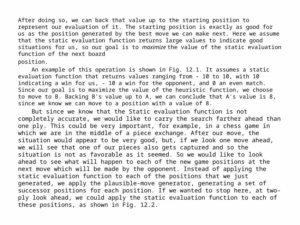
After doing so, we can back that value up to the starting position to represent our evaluation of it. The starting position is exactly as good for us as the position generated by the best move we can make next. Here we assume that the static evaluation function returns large values to indicate good situations for us, so our goal is to maximize the value of the static evaluation function of the next boardposition.

An example of this operation is shown in Fig. 12.1. It assumes a static evaluation function that returns values ranging from - 10 to 10, with 10 indicating a win for us, - 10 a win for the opponent, and 0 an even match. Since our goal is to maximize the value of the heuristic function, we choose to move to B. Backing B's value up to A, we can conclude that A's value is 8, since we know we can move to a position with a value of 8.

But since we know that the Static evaluation function is not completely accurate, we would like to carry the search farther ahead than one ply. This could be very important, for example, in a chess game in which we are in the middle of a piece exchange. After our move, the situation would appear to be very good, but, if we look one move ahead, we will see that one of our pieces also gets captured and so the situation is not as favorable as it seemed. So we would like to look ahead to see what will happen to each of the new game positions at the next move which will be made by the opponent. Instead of applying the static evaluation function to each of the positions that we just generated, we apply the plausible-move generator, generating a set of successor positions for each position. If we wanted to stop here, at two-ply look ahead, we could apply the static evaluation function to each of these positions, as shown in Fig. 12.2.

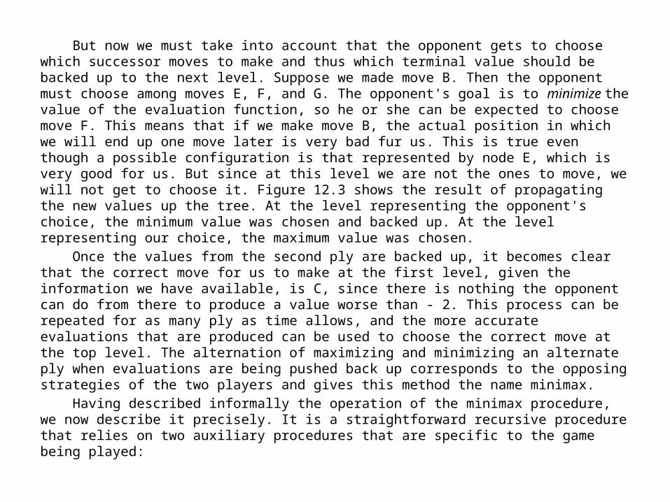
But now we must take into account that the opponent gets to choose which successor moves to make and thus which terminal value should be backed up to the next level. Suppose we made move B. Then the opponent must choose among moves E, F, and G. The opponent's goal is to minimize the value of the evaluation function, so he or she can be expected to choose move F. This means that if we make move B, the actual position in which we will end up one move later is very bad fur us. This is true even though a possible configuration is that represented by node E, which is very good for us. But since at this level we are not the ones to move, we will not get to choose it. Figure 12.3 shows the result of propagating the new values up the tree. At the level representing the opponent's choice, the minimum value was chosen and backed up. At the level representing our choice, the maximum value was chosen.

Once the values from the second ply are backed up, it becomes clear that the correct move for us to make at the first level, given the information we have available, is C, since there is nothing the opponent can do from there to produce a value worse than - 2. This process can be repeated for as many ply as time allows, and the more accurate evaluations that are produced can be used to choose the correct move at the top level. The alternation of maximizing and minimizing an alternate ply when evaluations are being pushed back up corresponds to the opposing strategies of the two players and gives this method the name minimax.

Having described informally the operation of the minimax procedure, we now describe it precisely. It is a straightforward recursive procedure that relies on two auxiliary procedures that are specific to the game being played:

1. MOVEGEN( Position , Player)-The plausible-move generator, which returns a list of nodes representing the moves that can be made by Player in Position. We call the two players PLAYER-ONE and PLAYER TWO ; in a chess program, we might use the names BLACK and WHITE instead.2. STATIC(Position , Player) -The static evaluation function, which returns a number representing thegoodness of Position from the standpoint of Player.As with any recursive program, a critical issue in the design of the MINIMAX procedure is when to stopthe recursion and simply call the static evaluation function. There are a variety of factors that may influence this decision. They include: • Has one side won? • How many ply have we already explored? • How promising is this path? • How much time is left? • How stable is the configuration?

For the general MINIMAX procedure discussed here, we appeal to a function, DEEP-ENOUGH, which is assumed to evaluate all of these factors and to return TRUE if the search should be stopped at the current level and FALSE otherwise. Our simple implementation of DEEP-ENOUGH will take two parameters, Position and Depth. It will ignore its Position parameter and simply return TRUE if its Depth parameter exceeds a constant cutoff value.

One problem that arises in defining MINIMAX as a recursive procedure is that it needs to return not one but two results :• The backed-up value of the path it chooses.• The path itself. We return the entire path even though probably only the first element, representing the best move from the current position, is actually needed.

We assume that MINIMAX returns a structure containing both results and that we have two functions , VALUE and PATH, that extract the separate components.

Since we define the MINIMAX procedure as a recursive function, we must also specify how it is to be called initially. It takes three parameters, a board position, the current depth of the search, and the player to move. So the initial call to compute the best move from the position CURRENT should be MINIMAX (CURRENT, 0 ,PLAYER-ONE)if PLAYER-ONE is to move, or MINIMAX (CURRENT, 0 ,PLAYER-TWO)if PLAYER-TWO is to move.Algorithm: MINIMAX(Position, Depth, Player)

1. If DEEP-ENOUGH(Position, Depth), then return the structureVALUE = STATIC(Position, Player);PATH = nilThis indicates that there is no path from this node and that its value is that determined by the static evaluation function.2. Otherwise, generate one more ply of the tree by calling the function MOVE-GEN(Position Player) and setting SUCCESSORS to the list it returns.3. If SUCCESSORS is empty, then there are no moves to be made, so return the same structure that would have been returned if DEEP-ENOUGH had returned true.

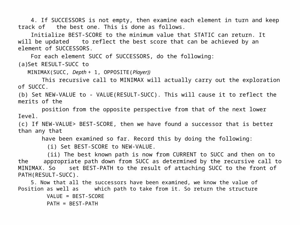
4. If SUCCESSORS is not empty, then examine each element in turn and keep track of the best one. This is done as follows. Initialize BEST-SCORE to the minimum value that STATIC can return. It will be updated to reflect the best score that can be achieved by an element of SUCCESSORS.For each element SUCC of SUCCESSORS, do the following:

(a) Set RESULT-SUCC to MINIMAX(SUCC, Depth + 1, OPPOSITE(Player))

This recursive call to MINIMAX will actually carry out the exploration of SUCCC.(b) Set NEW-VALUE to - VALUE(RESULT-SUCC). This will cause it to reflect the merits of the position from the opposite perspective from that of the next lower Ievel.(c) If NEW-VALUE> BEST-SCORE, then we have found a successor that is better than any that have been examined so far. Record this by doing the following: (i) Set BEST-SCORE to NEW-VALUE. (ii) The best known path is now from CURRENT to SUCC and then on to the appropriate path down from SUCC as determined by the recursive call to MINIMAX. So set BEST-PATH to the result of attaching SUCC to the front of PATH(RESULT-SUCC).

5. Now that all the successors have been examined, we know the value of Position as well as which path to take from it. So return the structure VALUE = BEST-SCORE PATH = BEST-PATH

When the initial call to MINIMAX returns, the best move from CURRENT is the first element on PATH. To see how this procedure works, you should trace its execution for the game tree shown in Fig. 12.2.

The MINIMAX procedure just described is very simple. But its performance can be improved significantly with a few refinements. Some of these are described in the next few sections.12.3 ADDING ALPHA-BETA CUTOFFS

Recall that the minimax procedure is a depth-first process. One path is explored as far as time allows, the static evaluation function is applied to the game positions at the last step of the path, and the value can then be passed up the path one level at a time. One of the good things about depth-first procedures is that their efficiency can often be improved by using branch-and-bound techniques in which partial solutions that are clearly worse than known solutions can be abandoned early. We described a straightforward application of this technique to the traveling salesman problem in Section 2.2.1. For that problem, all that was required was storage of the length of the best path found so far. If a later partial path outgrew that bound, it was abandoned. But just as it was necessary to modify our search procedure slightly to handle both maximizing and minimizing players , it is also necessary to modify the branch-and-bound strategy to include two bounds, one for each of the players. This modified strategy is called alpha-beta pruning. It requires the maintenance of two threshold values, one representing a lower bound on the value that a maximizing node may ultimately be assigned (we call this alpha) and another representing an upper bound on the value that a minimizing node may be assigned (this we call beta).

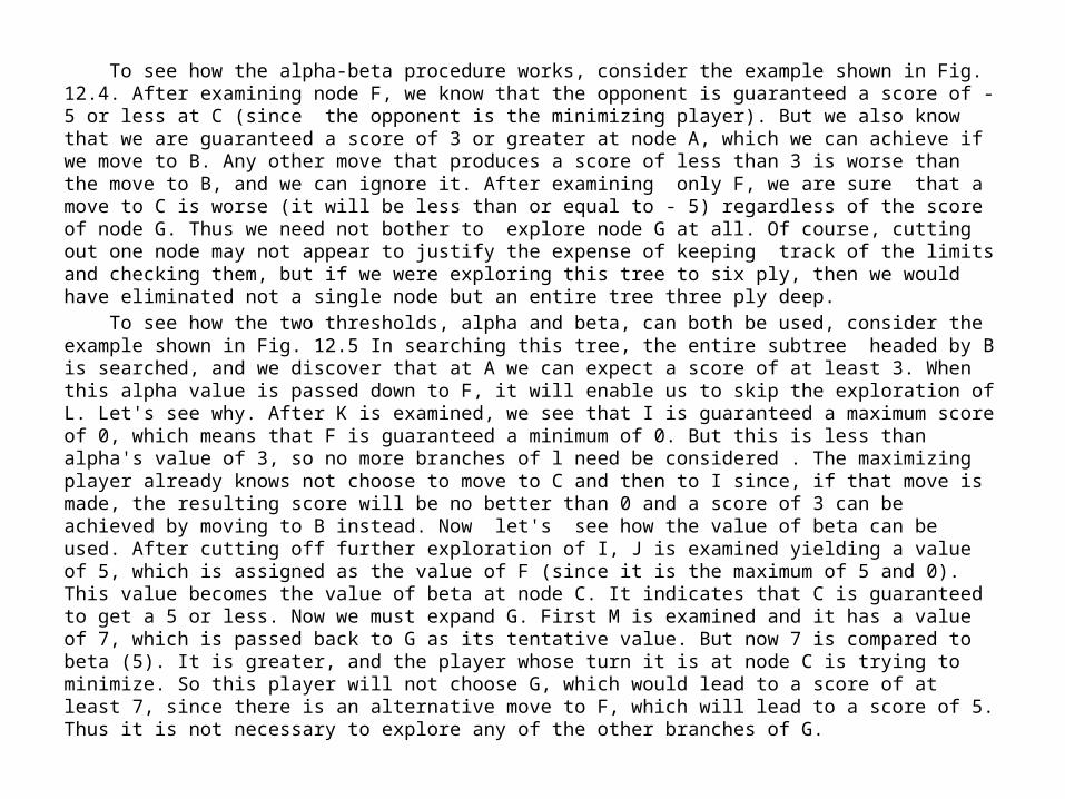
To see how the alpha-beta procedure works, consider the example shown in Fig. 12.4. After examining node F, we know that the opponent is guaranteed a score of -5 or less at C (since the opponent is the minimizing player). But we also know that we are guaranteed a score of 3 or greater at node A, which we can achieve if we move to B. Any other move that produces a score of less than 3 is worse than the move to B, and we can ignore it. After examining only F, we are sure that a move to C is worse (it will be less than or equal to - 5) regardless of the score of node G. Thus we need not bother to explore node G at all. Of course, cutting out one node may not appear to justify the expense of keeping track of the limits and checking them, but if we were exploring this tree to six ply, then we would have eliminated not a single node but an entire tree three ply deep.

To see how the two thresholds, alpha and beta, can both be used, consider the example shown in Fig. 12.5 In searching this tree, the entire subtree headed by B is searched, and we discover that at A we can expect a score of at least 3. When this alpha value is passed down to F, it will enable us to skip the exploration of L. Let's see why. After K is examined, we see that I is guaranteed a maximum score of 0, which means that F is guaranteed a minimum of 0. But this is less than alpha's value of 3, so no more branches of l need be considered . The maximizing player already knows not choose to move to C and then to I since, if that move is made, the resulting score will be no better than 0 and a score of 3 can be achieved by moving to B instead. Now let's see how the value of beta can be used. After cutting off further exploration of I, J is examined yielding a value of 5, which is assigned as the value of F (since it is the maximum of 5 and 0). This value becomes the value of beta at node C. It indicates that C is guaranteed to get a 5 or less. Now we must expand G. First M is examined and it has a value of 7, which is passed back to G as its tentative value. But now 7 is compared to beta (5). It is greater, and the player whose turn it is at node C is trying to minimize. So this player will not choose G, which would lead to a score of at least 7, since there is an alternative move to F, which will lead to a score of 5. Thus it is not necessary to explore any of the other branches of G.

From this example, we see that at maximizing levels, we can rule out a move early if it becomes clear that its value will be less than the current threshold, while at minimizing levels, search will be terminated if values that are greater than the current threshold are discovered. But ruling out a possible move by a maximizing player actually means cutting off the search at a minimizing level. Look again at the example in Fig. 12.4. Once we determine that C is a bad move from A, we cannot bother to explore G, or any other paths, at the minimizing level below C. So the way alpha and beta are actually used is that search at a minimizing level can be terminated when a value less than alpha is discovered, while a search at a maximizing level can be terminated when a value greater than beta has been found. Cutting off search at a maximizing level when a high value is found may seem counterintuitive at first, but if you keep in mind that we only get to a particular node at a maximizing level if the minimizing player at the level above chooses it, then it makes sense.

Having illustrated the operation of alpha-beta pruning with examples, we can now explore how the MINIMAX procedure described in Section 12.2 can be modified to exploit this technique. Notice that at maximizing levels, only beta is used to determine whether to cut off the search, and at minimizing levels only alpha is used. But at maximizing levels alpha must also be known since when a recursive call is made to MINIMAX, a minimizing level is created, which needs access to alpha. So at maximizing levels alpha must be known not so that it can be used but so that it can be passed down the tree. The same is true of minimizing levels with respect to beta. Each level must receive both values, one to use and one to pass down for the next level to use.

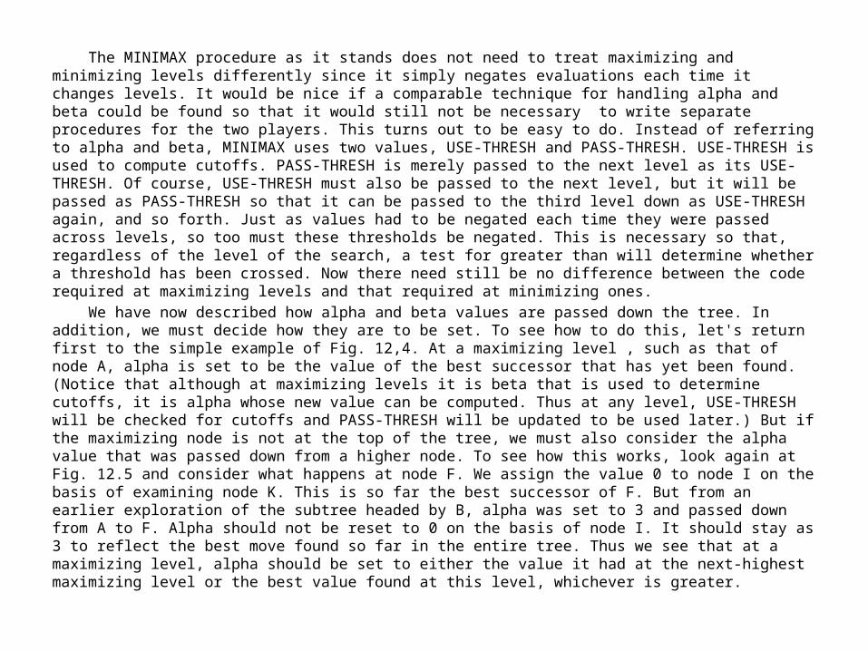
The MINIMAX procedure as it stands does not need to treat maximizing and minimizing levels differently since it simply negates evaluations each time it changes levels. It would be nice if a comparable technique for handling alpha and beta could be found so that it would still not be necessary to write separate procedures for the two players. This turns out to be easy to do. Instead of referring to alpha and beta, MINIMAX uses two values, USE-THRESH and PASS-THRESH. USE-THRESH is used to compute cutoffs. PASS-THRESH is merely passed to the next level as its USE-THRESH. Of course, USE-THRESH must also be passed to the next level, but it will be passed as PASS-THRESH so that it can be passed to the third level down as USE-THRESH again, and so forth. Just as values had to be negated each time they were passed across levels, so too must these thresholds be negated. This is necessary so that, regardless of the level of the search, a test for greater than will determine whether a threshold has been crossed. Now there need still be no difference between the code required at maximizing levels and that required at minimizing ones.

We have now described how alpha and beta values are passed down the tree. In addition, we must decide how they are to be set. To see how to do this, let's return first to the simple example of Fig. 12,4. At a maximizing level , such as that of node A, alpha is set to be the value of the best successor that has yet been found. (Notice that although at maximizing levels it is beta that is used to determine cutoffs, it is alpha whose new value can be computed. Thus at any level, USE-THRESH will be checked for cutoffs and PASS-THRESH will be updated to be used later.) But if the maximizing node is not at the top of the tree, we must also consider the alpha value that was passed down from a higher node. To see how this works, look again at Fig. 12.5 and consider what happens at node F. We assign the value 0 to node I on the basis of examining node K. This is so far the best successor of F. But from an earlier exploration of the subtree headed by B, alpha was set to 3 and passed down from A to F. Alpha should not be reset to 0 on the basis of node I. It should stay as 3 to reflect the best move found so far in the entire tree. Thus we see that at a maximizing level, alpha should be set to either the value it had at the next-highest maximizing level or the best value found at this level, whichever is greater.

The corresponding statement can be made about beta at minimizing levels. In fact, what we want to say is that at any level, PASS-THRESH should always be the maximum of the value it inherits from above and the best move found at its level. If PASS-THRESH is updated, the new value should be propagated both down to lower levels and back up to higher ones so that it always reflects the best move found anywhere in the tree.

At this point, we notice that we are doing the same thing in computing PASS-THRESH that we did in MlNlMAX to compute BEST-SCORE. We might as well eliminate BEST-SCORE and let PASS-THRESH serve in its place.

With these observations, we are in a position to describe the operation of the function MINlMAX-A-B, which requires four arguments, Position, Depth, Use-Thresh, and Pass-Thresh. The initial call, to choose a move for PLAYER-ONE from the position CURRENT, should be

MINIMAX-A-B(CURRENT. 0, PLAYER-ONE, maximum value STATIC can compute, minimum value STATIC can compute)These initial values for Use-Thresh and Pass-Thresh represent the worst values that each side could achieve.

Algorithm: MINIMAX-A-B( Position, Depth, Player, Use-Thresh, Pass-Thresh )1. If DEEP-ENOUGH(Position, Depth), then return the structure

VALUE = STATlC (Position, Player); PATH = nil

2. Otherwise, generate one more ply of the tree by calling the function MOVE- GEN(Position, Player) and setting SUCCESSORS to the list it returns.3.If SUCCESSORS is empty, there are no moves to be made; return the same structure

that would have been returned if DEEP-ENOUGH had returned TRUE.4. If SUCCESSORS is not empty, then go through it, examining each element and

keeping track of the best one. This is done as follows. For each clement SUCC of SUCCESSORS: (a) Set RESULT-SUCC to MINIMAX-A-B(SUCC, Depth + 1, OPPOSlTE (Player), - Pass-Thresh, - Use-Thresh). (b) Set NEW-VALUE to - VALUE(RESULT-SUCC). (c) If NEW-VALUE> Pass-Thresh, then we have found a successor that is better than any that have been examined so far. Record this by doing the following. (i) Set Pass-Thresh to NEW-VALUE. (ii) The best known path is now from CURRENT to SUCC and then on to the appropriate path from SUCC as determined by the recursive call to MINIMAX-A-B. So set BEST-PATH to the result of attaching SUCC to the front of PATH(RESULT-SUCC).

(d) If Pass-Thresh (reflecting the current best value) is not better than Use-Thresh, then we should stop examining this branch. But both thresholds and values have been inverted. So if Pass-Thresh >= Use-Thresh, then return immediately with the value VALUE = Pass-Thresh PATH = BEST-PATH5. Return the structure VALUE = Pass-Thresh PATH = BEST-PATH

The effectiveness of the alpha-beta procedure depends greatly on the order in which paths are examined. If the worst paths are examined first, then no cutoffs at all will occur. But, of course, if the best path were known in advance so that it could be guaranteed to be examined first, we would not need to bother with the search process. If, however, we knew how effective the pruning technique is in the perfect case, we would have an upper bound on its performance in other situations. It is possible to prove that if the nodes are perfectly ordered, then the number of terminal nodes considered by a search to depth d using alpha-beta pruning is approximately equal to twice the number of terminal nodes generated by a search to depth d/2 without alpha-beta [Knuth and Moore, 1975]. A doubling of the depth to which the search can be pursued is a significant gain. Even though all of this improvement cannot typically be realized, the alpha-beta technique is a significant improvement to the minimax search procedure. For a more detailed study of the average branching factor of the alpha-beta procedure, see Baudet [1978] and Pearl [1982].

The idea behind the alpha-beta procedure can be extended to cut off additional paths that appear to be at best only slight improvements over paths that have already been explored. In step 4(d), we cut off the search if the path we were exploring was not better than other paths already found. But consider the situation shown in Fig. 12.6. After examining node G, we see that the best we can hope for if we make move C is a score of 3.2. We know that if we make move B we are guaranteed a score of 3.

Since 3.2 is only very slightly better than 3, we should perhaps terminate our exploration of C now. We could then devote more time to exploring other parts of the tree where there may be more to gain. Terminating the exploration of a subtree that offers little possibility for improvement over other known paths is called a futility cutoff.12.4 ADDITIONAL REFINEMENTS

In addition to alpha-beta pruning, there are a variety of other modifications to the minimax procedure that can also improve its performance. Four of them are discussed briefly in this section, and we discuss one other important modification in the next section.12.4.1 Waiting for Quiescence

As we suggested above, one of the factors that should sometimes be considered in determining when to stop going deeper in the search tree is whether the situation is relatively stable. Consider the tree shown in Fig. 12.7. Suppose that when node B is expanded one more level , the result is that shown in Fig. 12.8. When we looked one move ahead, our estimate of the worth of B changed drastically. This might happen, for example, in the middle of a piece exchange. The opponent has significantly improved the immediate appearance of his or her position by initiating a piece exchange. If we stop exploring the tree at this level, we assign the value - 4 to B and therefore decide that B is not a good move.

To make sure that such short-term measures do not unduly influence our choice of move, we should continue the search until no such drastic change occurs from one level to the next. This is called waiting for quiescence. If we do that, we might get the situation shown in Fig. 12.9, in which the move to B again looks like a reasonable move for us to make since the other half of the piece exchange has occurred. A very general algorithm for quiescence can be found in Beal [1990].

Waiting for quiescence helps in avoiding the horizon effect, in which an inevitable bad event can be delayed by various tactics until it does not appear in the portion of the game tree that minimax explores. The horizon effect can also influence a program's perception of good moves. The effect may make a move look good despite the fact that the move might be better if delayed past the horizon. Even with quiescence, all fixed depth search programs are subject to subtle horizon effects.