g1ig copn - apps.dtic.mil
TRANSCRIPT

g1Ig IE COPN 4 •
DEVELOPMENT AND TESTING OF RAPIDREPAIR METHODS FOR WAR DAMAGED RUNWAYS
0
BY
NPAUL A. SOARESN
DTICELECTE
SJUL18199011
A REPORT PRESENTED TO THE GRADUATE COMMITTEEOF THE DEPARTMENT OF CIVIL ENGINEERING IN
PARTIAL FULFILLMENT OF THE REQUIREMENTSFOR TH'. DEGREE OF MASTER OF ENGINEERING
UNIVERSITY OF FLORIDA
Spring 1990
[-i§TRMBTION STATM AA.
Approv•d for public releas;Distribuon Uilmite0d
90 0 77 04A1
I DEVELOPMENT AND TESTING OF RAPIDREPAIR METHODS FOR WAR DAMAGED RUNWAYS
BY
PAUL A. SOARES
I A REPORT PRESENTED TO THE GRADUATE COMMITTEEOF iIHE DEPARTMENT OF CIVIL ENGINEERING INPARTIAL FULFILLMENT OF THE REQUIREMENTS
FOR THE DEGREE OF MASTER OF ENGINEERING
UNIVERSITY OF FLORIDA
Spring 1990
DISTRMUTION STAtMEN= A
Approved for public release;'istribution UnlimitedDitibto Unlimite

DEDICATION
This report is dedicated to my beautiful wife,
Kathleen, for all of her loving support through these
two years of postgraduate school.
Accession For..NTIS GRA&I '
DTIC TABUnannounced ]
Distribution/ '
Availability Codes01Avail and/or '
Dist Special
a ____ _i_
ACKNOWLEDGEMENTS
Sincere gratitude is extended to Dr. David
Bloomquist for all of his assistance and guidance
throughout the entire length of this research in
determining and verifying the mix design procedures.
Special acknowledgement and thanks is also extended
to Professor Will Shafer and Doctor Ralph Ellis for
their assistance and guidance in preparing this
report.
A special thanks to Dr. Fagundo for assisting in
the development and evaluation of the initial ideas
of this research. The author wishes to express
appreciation to Dr. Byron E. Ruth for his interest
and guidance in developing mix design approaches.
The author extends special gratitude to Mr.
Charles Allen for providing vital information on
aggregate properties vital to performing this
research.
The author sincerely thanks Mr. Daniel
Richardson for his super assistance in the Civil
Engineering Materials Laboratory.
The author acknowledges the integral assistance
of the Florida Department of Transportation,
especially to Mr. Toby Larson and Dr. Armaghani
A special thanks to Mr. Richard Coble for
working in conjunction with me to provide knowledge
of construction equipment capabilities and procedures
(ii)

as well as actual construction equipment, materials,
skilled equipment operators, a testsite, and funding
needed to complete the field test.
(iii)
II
PREFACE
IThe problem of effecting repair to war damaged
runways within the time constraints of a combat
situation currently looms at large for the Armed
Services of the United States. Although several
methods have been proposed and tested, none have been
I adopted as the answer to the problem. Research
continues on in earnest at several Department of
Defense Research Centers.
As a Naval Officer with 2.5 years of hands-on
experience in effecting repair to war damaged
I runways, I chose this subject as the basis for my
Master's Report. After consulting with several
prominent professors and engineers, I had gathered
several solutions to the problem. One concept that
looked very promising was conceived through
I consultation with Mr. Richard Coble.
iMr. Coble is attending the University of Florida
to obtain a PH.D. in Architecture. Mr. Coble is
president of KACO Construction Company which performs
approximately IS million dollars worth of
I construction annually. Mr. Coble has a Bachelor of
Science Civil Engineering and Master's Degree in
Building Construction.
The concept involves mixing the materials in
place. My work began with developing a mix design
3 utilizing roller compacted concrete technology. I
(iv)

II
also formed rough ideas as to how the method could be
developed into a construction technique.
With my construction ideas, I consulted with Mr.
Coble as to the validity of the techniques. Due to
his 25 yrs of contracting experience, with emphasis
in equipment and soil stabilization, he was able to
evaluate my ideas and develop additional ideas to
form a construction method.
At this point, I looked toward development of a
I lab test on the smallest scale possible, that would
I still simulate the actual conditions of the real
scenario of repairing war damaged runways. I would
face the limitations of how close the simulation
would come to the real construction operation.
I Upon further consultation with Mr. Coble, an
i agreement was reached to conduct a full scale test as
a joint research effort between myself and Mr. Coble.
The Joint effort would involve the pooling of my
experience as Naval Officer working in war damage
I repair and equipment management, along with Mr.
Coble's experience as a general contractor
specializing in equipment management.
The test would have the resources of Mr. Coble's
Company, KACO Construction, at its disposal including
3 a test site to perform the full scale test. The
resources included all necessary equipment,
(v)I

operators, materials, computers, video equipment, and
other resources that would not have been otherwise
available.
Therefore, through the teaming of my naval
experience and engineering knowledge along with Mr.
Coble's experience in equipment capabilities,
construction techniques, and the resources of KACO
Construction Company, the research progressed at a
pace which completed all design, development,
testing, and verification of results on a large scale
test within a four month timeframe.
The successful completion of this research can
only be attributed to the diverse backgrounds of each
partner coming together to form a competent team.
Each partner obtained vital information from several
I sources including prominent professors and engineers.
The preparation of this report covers the work
completed by myself for the fulfillment of the
requirements of my master's degree. The information
and materials obtained through Mr. Coble, along with
i all other sources, are noted in the reference
section.
(vi)
TABLE OF CONTENTS
LIST OF TABLES x
LIST OF FIGURES xii
CHAPTERS
1. INTRODUCTION 1
1.1 Problem Statement 11.2 Study Objectives 31.3 Scope of Work 3
2. FIELD TEST PROCEDURE S
2.1 Construction Sequence S2.1.1 Master Activity Listing 52.1.2 Construction Sequence 8
Conditions2.1.3 Construction Sequence 8
Discussion2.2 Water Application 26
2.2.1 Determining Flowrate 262.2.2 Determining Velocity 282.2.3 Measuring Velocity 322.2.1 Foul Weather Procedure 332.2.5 Calcium Chloride Application 35
3. MIX DESIGN DEVELOPMENT 36
3.1 Material Parameters 363.1.1 Mix Design and Moist Rodded 36
Unit Weight CMRUW) InputValues
3.1.1.1 MRUW Test 373.1.1.2 MRUW Calculations 38
3.1.2 Analysis of Agrregate L10
Parameters3.1.2.1 Verifying MRUW 423.1.2.2 MRUW Ranges 443.1.2.3 Void Ratios 443.1.2.q Aggregate Parameter 55
Ranges3.2 Proportioning of Mix Design Li5
3.2.1 Calculating Proportions by LiAbsolute Volume in Mix
3.2.2 Converting Absolute Volumes 47to Saturated Surface Dry(SSD) Weights
3.2.3 Converting SSD Weights to 58Natural Moisture ContentCNMC) Weights
(vii)
3.2.1 Calculating the Water/Cement 51(W/C) Ratio and MoistureContent of Mix
L. LAYER THICKNESS CALCULATION 53
4.1 Introduction 53q.2 Converting NMC Weight Proportions to 54
Pre-Nix Volumesq.3 Converting Pre-Mlix Volumes to Layer 56
ThicknessesLi.3.1 Calculating Crater Type and 56
Size4.3.1.1 Circular Crater 56
Parametersq.3.1.2 Rectangular Crater 61
Parameters4.3.1.3 Irregular Crater 63
Parametersq.3.1.i External Equivalent 63
Hole Parametersf.3.2 Calculating Pre-Mix Layer 66
Thicknesses4.3.3 Angle of Repose 67f.3.4 Calculating Angle of Repose 66
Layer Thicknessei34.4 Calculating Spacing of Cement Bags 75q.5 Volume Reduction Percentages 76
5. QUALITY VERIFICATION 79
5.1 Introduction 795.2 Settlement Tests 805.3 Laboratory Testing of Laboratory 83
Mixed and Compacted Test Specimens5.4 Laboratory Testing of Field Mixed and 89
Laboratory Compacted Test Specimens5.5 Laboratory Testing of Field Mixed and 95
Compacted Test Specimens.5.6 Comparison of Laboratory Mixed and 97
Compacted, Field Mixed and LaboratoryCompacted, and Field Mixed andCompacted Test Specimens5.6.1 Compressive Strength Versus 100
Compaction %5.6.2 Compressive Strength Versus 109
Time
6. SENSITIVITY ANALYSIS 1226.1 Introduction 1226.2 MRUW Values to Layer Thickness 122
Relationship6.3 Total Water Application to W/C Ratio 12Lf
and Moisture Content Relationship.
(viii)
I
I 7. CONCLUSIONS AND RECOMMENDATIONS 126
7.1 Conclusions 1267.2 Recommendations 129
APPENDICES
A Flow Container Calculations for 133Trapezoidal Container
B Calcium Chloride Application 135
3 C Material Requirements 136
0 Universal Engineering Test Results 137
E Concrete Test Results 1i2
F Compressive Strength Graph Data 143
REFERENCES 146
IIIIIIIII
Cix)I

I
I eLIST OF TABLES
I 2.1 Water Volumes and Times 26
2,2 Watertruck Parameters 30
2.3 Testhole Parameters 31
3.1 Aggregate Parameters 37
3.2 Moist Rodded Unit Weight Test Results 39
I 3.3 Mix Design Variables 4i
3.1f Aggregate Parameter Ranges Li
I 3.5 Actual Mix Design Summary (l cy) 50
3.6 Volumes and Weights of Ingredients 51
i.1 Circular Crater Parameters 56
L•.2 Volume Reduction for Equivalent Hole 59
4.3 Actual and Equivalent Parameters of 653 Testhole
4.4 Actual Mix Design Summary 66
3 •.5 Angles oF Repose 68
4.6 Angle of Repose Variable Definitions 69IL.7 Coarse Aggregate Quadratic Terms 71
L•,B Coarse Aggregate Quadratic Terms and 71
Root Values
I .5 Fine Aggregate Quadratic Terms 73
I.10 Fine Aggregate Quadratic Terms and 74Root Values
4.,11 Layer Thicknesses 75
1 *.12 Cement Powder Data 75
4.13 Cement Bag Spacing 76
4 .14I Layer Thickness Comparison 78
S.1 Settlements of Plate Load Test 83
ICx)I
I
1 5.2 Laboratory Cylinder Corrected Compressive 8S
Stress
5.3 Laboratory Cylinder Compressive Strength 86Data Sheet
5.• Laboratory Cylinder Tensile Unit Weight 87and Compaction
5.5 Laboratory Cylinder Tensile Strength 87
5.6 Laboratory Flexural Beam Dimensions and B8* Unit Weight
5.7 Laboratory Beam Flexural Stress 88
35.6 Laboratory Beam Curing Time 88
5.9 Field Cylinder Corrected Compressive 93* Stresses
5.10 Field Cylinder Compressive Strength 95Data Sheet
5.11 Field Core Corrected Compressive Stresses 96
.5.12 Field Core Compressive Strength Data Sheet 96
5.13 Summary of All Actual Strengths 97
35.1I Stress Relationships 98
5.15 Actual and Calculated Stress Ualues 99
5.16 Mean Compressive Stresses 110
5.17 Compaction and Compressive Strength 112Averages (Lab Mixed and Compacted)
5.18 Compaction and Compressive Strength 115Averages (Field Mixed and Lab Compacted)
5.19 Compaction and Compressive Strength 1183 Averages (Field Mixed and Compacted)
6.1 Coarse Aggregate MRUW Sensitivity Analysis 122
36.2 Fine Aggregate MRUW Sensitivity Analysis 123
6.3 Flowrate Sensitivity Analysis 1•
6.i Watertruck Speed Sensitivity Analysis 125
(xi)I

LIST OF FIGURES
Ficure
2.1 CPM Diagram 7
2.2 Marked Off Area CEquivalent Hole) 9
2.3 Partial Coarse Aggregate Placement 11
2.1f Front End Loader Placing Coarse Aggregate 11
2.5 Leveling Off Coarse Aggregate 12
2.6 Measuring Coarse Aggregate Layer 12
2.7 Cement Bag Placement i4
2.8 Cement Powder Placement With Sand Cover ii
2.9 Sand Leveling Off and Measuring is
2.10 Soil Stabilizer Placement 16
2.11 Soil Stabilizer Mixing Tines 16
2.12 Dry Mixing of Aggregates and Cement Powder 17
2.13 Lip Formation 18
2.14 Water Application 18
2.15 Water Run-Off 20
2.16 Grader Windrowing Wet Material 20
2.17 Repositioning Soil Stabilizer 21
2.18 Wet Mixing of Aggregates and Cement Powder 21
2.19 Grader Windrowing Wet Mixed Material 22(Front Uiew)
2.20 Grader Windrowing Wet Mixed Material 22CSide Uiew)
2.21 Additional Water Placement 21
2.22 Vibratory Roller and Entire Slab View 2f
2.23 Uibratory Roller and Partial Slab View 25
2.21 Vibratory Roller CClose-up View) 25
(xii)

2.25 Water Container Filling (Trial 1) 27
2.26 Water Container Filling (Trial 1) 27
2.27 Depth Measurement 28
3.1 Phase Diagram Relationships 42
4.1 Circular Crater Equivalent Hole 58
Lt.2 Uolume Reductions for Equivalen.- Hole 60
t.3 Rectangular Crater Equivalent Hole 62
•.4 Order of Aggregate Placements 69
5.1 Placement of Plate Load 81
5.2 Load Plate (100 psi) 81
5.3 Fully Loaded Load Plate (400 psi) 82
5.Li Mixed, Uncompacted Slab 90
5.5 Cylinder Vibration 90
5.6 Cylinder Compaction 91
5.7 Sawcut Test Cylinders 91
5.8 Cylinder and Cylinder Capping Mold 92
5.9 Compressive Test Performance 9L1
5.10 Compressive Strength Us. Compaction at 1012q hrs (Lab Mixed and Compacted)
5.11 Compressive Strength Us. Compaction at 1028 days (Lab Mixed and Compacted)
5.12 Compressive Strength Us. Compaction at 10414 hrs (Field Mixed and Lab Compacted)
5.13 Compressiva Strength Us. Compaction at 1052q hrs (Field Mixed and Lab Compacted)
5.14 Compressive Strength Us. Compaction at 1073 days (Field Mixed and Compacted)
5.15 Compressive Strength Us. Compaction at 1087 days (Field Mixed and Compacted)
(xiii)

5.16 Individual Cylinder Compaction% Us. illAverage Compaction% (Lab Mixed andCompacted)
5.17 Compressive Strength Us. Time (Lab Mixed 113and Compacted)
5.18 Individual Cylinder Compaction% Us. ii4Average Compaction% (Field Mixed and LabCompacted)
S.19 Compressive Strength Us. Time (Field 116Mixed and Lab Compacted)
5.20 Individual Cylinder Compaction% Us. 117Average Compaction% (Field Mixed andCompacted)
5.21 Compressive Strength Us. Time (Field 119Mixed and Compacted)
5.22 Compressive Strength Us. Time (All 121Samples)
(xiv)

CHAPTER 1
INTRODUCTION
1.1 Problem Statement
In a combat/hostile scenario, the USAF main
operating bases CMOBs) and U.S. Naval Air Stations
(NAUAIRSTA) must function efficiently and effectively
despite runway damage. The MOBs must support tactical
aircraft launch and recovery Ml). The NAVAIRSTAs must
provide critical logistics support to the fleet, forward
deployed antisubmarine warfare CASW) aircraft bases, and
alternative launch and recovery sites for carrier aircraft
C(2). Because of the important functions served by MOBs and
NAUAIRSTAs, they will become primary targets for enemy
and/or terrorist forces. The damage sustained from enemy
and/or terrorist forces must be repaired in a rapid and
effective manner.
The term rapid is typically interpreted to mean within
21 hrs, however, many cases will require repair in less than
2'* hrs Ci.e. returning aircraft that cannot be diverted).
The term damage is typically interpreted to include craters
and spalls (small holes not completely through the slab).
The current rapid repair methods include using crushed
stone with some type of cover to prevent loosened stones
From entering Jet engine intakes to cause foreign object
damage (FOD) to the engine turbines. The types of FOD
covers are Fiber reinforced Polyester (FRP) mats, AM-2
matting, precast concrete slabs, and quickset concrete
utilizing a Cretemobile to batch the concrete (3).
Cl)

Each type of FOD cover has unique disadvantages. The
FRP mats are constantly being researched to improve their
anchoring capability. The significant problem is that the
mats do break loose from their anchoring due to lateral
forces imparted onto the mats by high speed contact with
aircraft landing gear. Sliding FRP mats could cause damage
to aircraft landing gear during landings. Also, loose
stone escapes from areas of the backfilled crater that are
exposed due to the sliding mat. The FRP mats do not provide
any structural support for the crushed stone, therefore, the
crushed stone base ruts from aircraft traffic creating a
need for the FRP mats to be removed for routine leveling and
compacting of the crushed stone base.
The AM-2 matting is an interlocking steel plate system.
A plate can be placed manually by two men. The 1.S"
thickness of the plates causes a jolt to aircraft landing
gear when they traverse from existing pavement onto the AM-2
matting. The jolt is beyond the cyclic loading tolerance
for landing gear of the Navy F-3, Air Force F-15, and F-16
aircraft (q). The aircraft type restriction renders AM-2
almost useless for main runway repair.
Precast concrete slabs are placed by construction
equipment. The slabs are typically two meter squares with a
depth of 6 inches CS). The precast slabs typically undergo
differential settlement from slab to slab. The time
required for cutting old concrete and heavy equipment
required for placement of slabs along with differential
C2)

settlement makes the precast slab method undesirable for
main runway repair.
The use of quickset concrete requires time to attain an
initial set from the plastic state of wet concrete. The
quickset concrete method also requires the use of a
Cretemobile which is a truck with a small batch plant
capable of producing approximately 25 CY/hour (6). The
output is directly controlled (critical path) by the number
of Cretemobiles onsite. The initial time of non-use, due to
6the plastic state of the wet concrete, and the limited
Cretemobile output makes the quickset concrete method
difficult to utilize as a main runway repair method.
A need exists to establish a main runway repair method
that is rapid, effective, and easy to install.ý
1.2 Studu Oblectives
The primary objective of this research was to develop a
rapi-d runway repair method that could be implemented by the
armed forces within their current resources.
1.3 Scope of Work _ -
A meth~d of mixing fine aggregate, coarse aggregate,
cement, and water was developed using soil stabilizing
equipment.
The required testslab thickness was selected from known
slab thicknesses in existence today. The mix design was
developed for a roller compacted mix. The mix design was
tested in a laboratory for compressive, tensile and flexural
strength. Simplified relationships were developed between
(3)

the degree of compaction versus the strength of concrete.
Moist Rodded Unit Weight tests were performed on the
fine and coarse aggregates to determine a pre-mix unit
weight of each material. The mix proportions by weight of
fine aggregate, coarse aggregate, and cement were converted
to pre-mix volumes. An angle of repose test was performed
on the fine and coarse aggregates. The pre-mix volumes were
converted to layer thicknesses.
CA field test procedure was developed to conduct a large
scale test of the method. A large scale test was performed.
Settlement tests were conducted on an hourly basis to
determine the rate of settlement versus time relationship.
Test specimens of concrete material were collected and
tested for compressive strength./
Flexural and tensile strengths were calculated usipg
known conservative compressive to flexural strengthh
relationships. Analysis was performed to deter ine the
degree of compaction versus the str n relationships at
different times of curin
Conclusions re drawn as to the overall suitability of
this methqo-"'for main runway repair. Finally, several/
recommendations were made for areas were further research//
could/be conducted for this method.
/77/1
N~)
CHAPTER 2
FIELD TEST PROCEDURE
2.1 Construction Sequence
2.1.1 Master Activitu Listing
The critical path activities were developed through
consultation with Rick Coble, President of KACO construction
company (7).
The critical path activities in the construction
sequence were as follows:
1. MARK-OFF HOLE; Mark-off equivalent hole
2. PLACE COARSE LAYER; Fill-in and level off coarse
layer
3. PLACE CEMENT; Lay cement bags down at proper
intervals. Open cement bags and spread out powder
in thin layer. Place small amount of sand
simultaneously on top of cement powder.
Lt. PLACE FINE LAYER; Place sand on top of cement and
level off to desired height.
5. BLEND DRY MIX; Mix aggregates and cement together
with soil stabilizer.
6. FORM LIP AND GROOUES; Form lip around mixed
materials and make grooves in material
perpendicular to the slope of existing ground.
7. APPLY WATER; Apply water by watertruck.
B. WINDROW EDGES IN; Windrow edges of layers towards
center of layers with a motor-grader.
S. BLEND WET MIX; Mix water, aggregates, and cement
together with mixer.
(5)
10. FILL HOLE; Blade material into hole with grader
11. WET DRY SPOTS; ApplW water with a hose in small
quantities as grader blades material into hole.
12. COMPACTION; Compact with roller.
13. REMOUE EXCESS; Grade ofF excess with grader.
14. FINISH ROLL; Make final roller pass to obtain
smooth Finish
The CPM diagram is shown in Figure 2.1.
I
I6

U-) U-)
r.-- U
C, A
uli ,al U-3 Ifl a
a) i.C L3 _z
W') Loi Ui (flO j 0
Si - i ..-..0 0 4.i
10 1*
4 C1 I' -00 Lii
In-
-W L. USiý 4-o c
CL-
Ln.
£: >
U' C- L. 1- ai4.i L- CUC -
-j IU 0 ~-o, -0 Ciý 4-i =i
U')4. Lo L. 03 in a4- 0ýLJ -
CD Li
U-3a L" I) L, La. -J
U-) . Cý C- a- m LLLkLU
ap $.- 3C> I > LnLU <
UU
C> 7)

2.1.2 Construction Sequence Conditions
3 The conditions before performing the first master
activity were:
1. The layer depths were already calculated.
g The base laWer width and length were calculated, More
discussion on layer dimension calculations is contained in
3chapters 3 & 4.
2. The crater was backfilled to a uniformd depth of 8
£ inches and compacted.
* 3. The area surrounding the crater was paved.
2.1.3 Construction Sequence Discussion
All photographs used as figures in this section were
taken and developed by Rick Coble of KACO construction
company (8). Through the use of a stringline, an area to
place the material was marked off that was outside of the
crater. This marked off area or box is shown in Figure 2.2.
iJI,
I
3 C8)

Ii
Figure 2.2 Marked Off Area (Equivalent Hole)
(9)

The coarse aggregate was placed first into the marked
off box. The use of the marked off box to place the
material in rather than placing the material directly into
3 the hole is called the equivalent hole concept. Furt•3r
discussion on the equivalent hole concept is contained in
chapter 4. The keypoint to understand at this point is that
the material placed above ground in the marked off box
was the amount plus waste required to fill the testhole.
Figures 2.3 and 2.4 show the coarse aggregate filling
operation. The coarse aggregate was placed forming a
trapezoid up to a depth of 5.25 inches (approximately equal
to exact calculated depth of 5.3 inches). Figures 2.5 and
2.6 show the measuring operation. The layer depth
calculations for all layers are contained in chapter 4.
(
C 10)
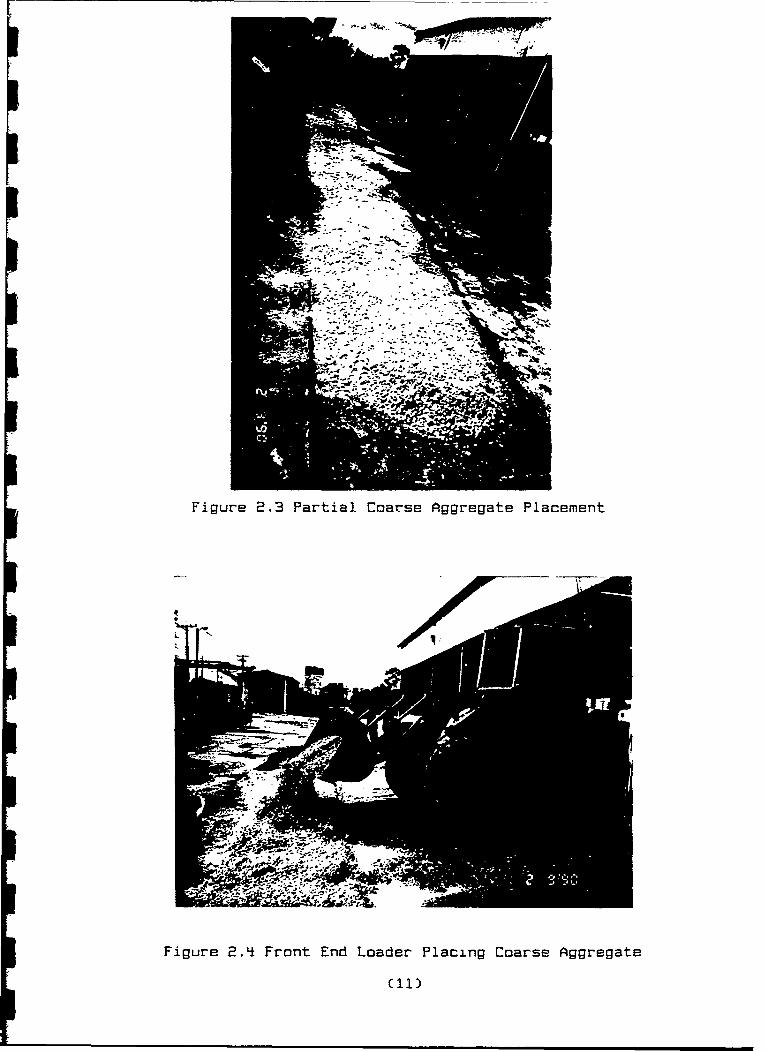
Figur-e 2.3 Partial Coar-se Aggregate Placement
Figure 2.4i Front End Loader Placing Coarse Aggregate

Figure 2.5 Leveling Off Coarse Aggregate
Figure 2.6 rleasur-ing Coarse Aggregate Layer
(12)

The cement bags were spaced apart at 2 ft 6 inches as
shown in Figure 2.7. The cemsnt bag spacing calculations
are covered in section 4.4. The cement bags were opened and
spread by hand. Small amounts of sand were simultaneously
placed on top of the cement powder to prevent the wind from
blowing away the cement powder. Figure 2.8 shows the cement
anO sand placing operation at completion.
(13)

Figur~e 2.7 Cement Bag Placement
Figure 2.8 Cement Powder Placement With Sand Cover
Ci14)

Place fine aggregate (sand) layer up to desired height.
Figure 2.9 shows sand leveling off operation.
I
Figure 2.9 Sand Leveling Off and Measuring
The soil stabilizer was then positioned at one end of
3l the layers as shown in Figures 2.9 & 2.10. The mixing
action was accomplished by the mixing tines as shown in
Figure 2.11.
LtiE

SIR
Figure 2.10 Soil Stabilizer Placement
Figur-e 2.11 Soil Stabilizer- Mixing Tines
16)
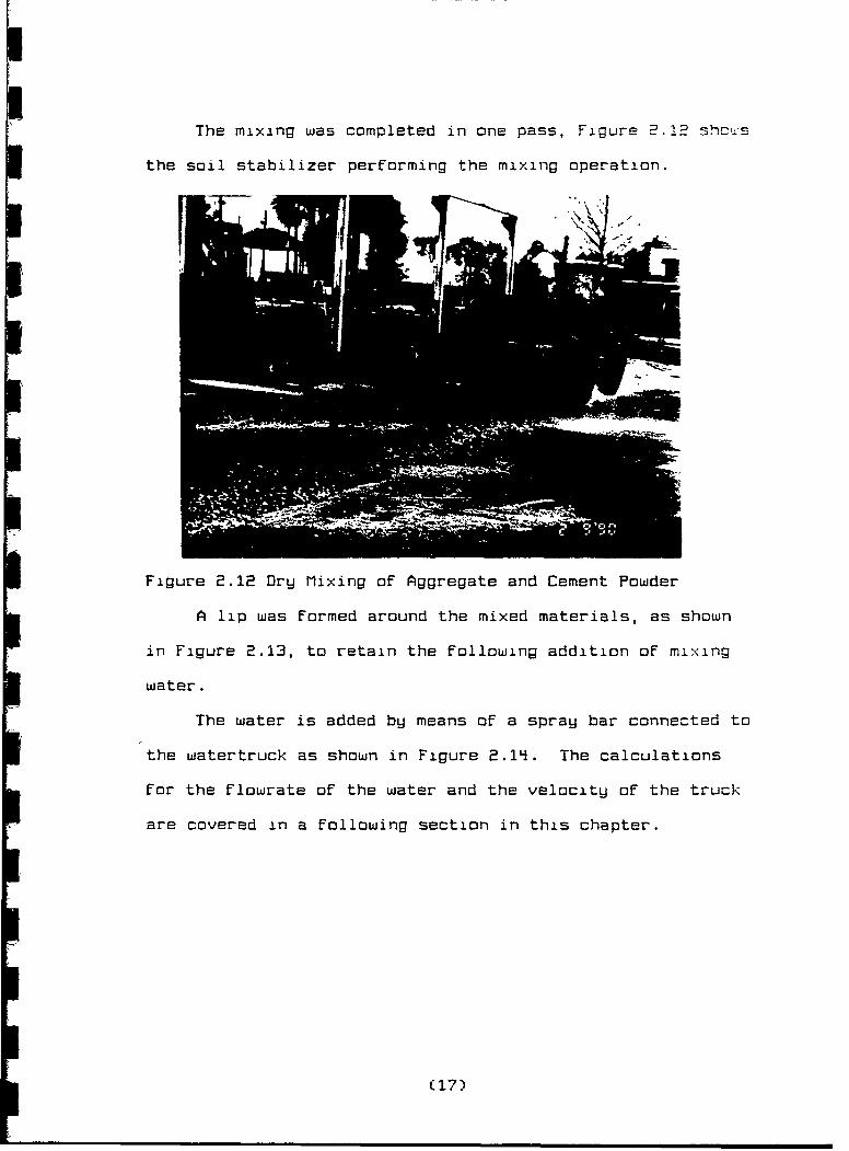
The mixing was completed in one pass, Figure 2.12 shcts
the soil stabilizer performing the mixing operation.
Figure 2.12 Dry Mixing of Aggregate and Cement Powder
A lip was formed around the mixed materials, as shown
in Figure 2.13, to retain the following addition of mixing
water.
The water is added by means of a spray bar connected to
the watertruck as shown in Figure 2.14. The calculations
for the flowrate of the water and the velocity of the truck
are covered in a following section in this chapter.
(17)

IUI
IIIII
FiQure 2.13 Lip Formation
p£
IIIIII3 Figure 2.1� Water �pp1ication
(18)

A field discovery and modification of the technique was
the scoring of the surface of the layers. A scoring
technique must be used to make grooves in the material
perpendicular to the slope of existing ground. This will
allow water to reach the lower depths of the mixed
materials. Otherwise, the material becomes saturated near
the top only before becoming impermeable due to water
surface tension causing tight adhesion between particles.
This temporary impermeability will cause some mixing water
to run off of the layers onto the surrounding ground, as
shown in Figure 2.1S, thereby, leaving mixed material at
lower depths completely dry.
A deviation from the actual procedure used in the field
will be recommended here. It is recommended that a
motor-grader be used, before the first mixing, to windrow
the edges of the layers back into the center of the lagers.
This is recommended because the edges are typically dry due
to the necessary retention of water towards the center of
the layers by the containment lip to prevent water run-off.
Once the pooled water seeps into the lower center of the
mixed material layer, the dry edges should be windrowed into
the center to allow improved mixing by the soil stabilizer.
During the field test the wet material was mixed first and
then the edges were windrowed in afterwards as shown in
Figure 2.16. This necessitated an extra pass by the soil
stabilizer to mix in dry edges windrowed into the
center.
(19)

Figure 2.1S Water Run-OFF
Figure 2.16 Grader Windr-owing Wet Mlaterial
(20)

The soil stabilizer- was positioned and then run over
the wet windrowed material as shown in Figures 2.17 g2.18.
Figure 2.17 Repositioning Soil Stabilizer
Figure 2.16 Wet Mlixing of Aggregate and Cement Powder
( 21):
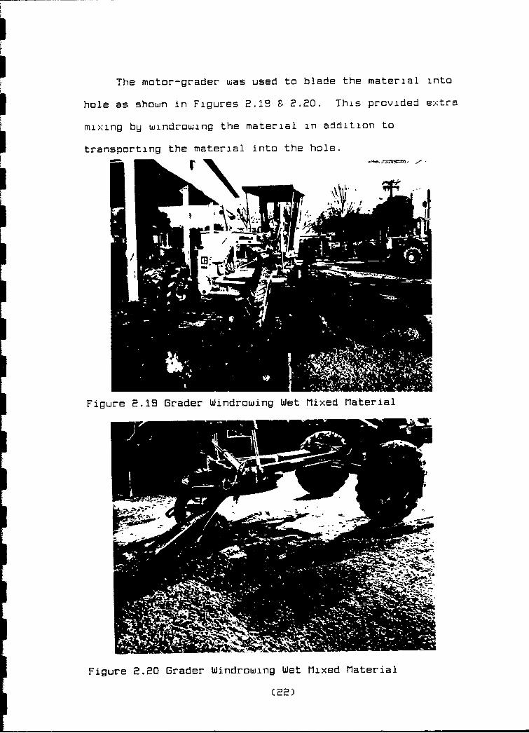
The motor-grader was used to blade the material into
flhole as shown in Figures 2.19 & 2.20. This provided extra
mixing by windrowing the material in addition to
I transporting the material into the hole.
Figure 2.19 Grader Windrowing Wet Mlixed Mlaterial
Figure 2.20 Grader Windrowing Wet Mlixed Miaterial
(22)
II
Water was added to exceptionally dry areas by means of
a hose as shown in Figure 2.21. Further discussion
concerning permissible quantities of water that can be added
by hose are discussed in following sections in this chapter.
The addition of water was performed while the motor-grader
was blading the material into the crater.
* The material was compacted by means of a smooth drum
vibratory roller. Several passes were made over the
I material as shown in Figures 2.22 & 2.23. The total time of
compaction was approximately 15 minutes. The material
deformed slightly (less than 1 inch) under vibratory
compaction as shown in Figure 2.2q. Overall, the material
exhibited very good stiffness.
I The material that remained above the desired elevation
of the slab was graded off using the motor-grader.
One pass with the roller was made with no vibration to
smooth out the final finish of slab.
IIIII
hO
Figure 2.21 Additional Water Placement
Figure 2.22 Vibratory Roller and Entire Slab Viaew
(24i)
IC
Fiue22Iirtr ole n ata lbVe
Fiue22Uirtr Rle CoeU iwI2S

2.2 Water Application
The calculations for the application of water to the
dry mixed layers will be discussed in this section. The
First step was the calculation of flowrate.
2.2.1 Determinina Flowrate
To determine the flowrate of the watertruck, the water
truck was backed up to a trapezoidal container. Two
trials of filling the containers were performed. In trial
1, the spray bar was placed over the container, the water
was turned on and allowed to fill the container as shown in
Figure 2.25. The water was turned off without moving the
truck. In trial 2, the truck was driven off to discontinue
water flow into the container as shown in Figure 2.26. The
time required to fill the container in each trial was
measured and recorded. The volume of water in the filled
container was calculated by measuring the depths as shown in
Figure 2.27. The volume calculations are contained in
Appendix A.
The volumes of water and times were recorded for two
trials. The average of the two volumes and times were used
to calculate the flowrate. Table 2.1 shows the values
recorded.
Table 2.1 Water Uolumes and Times
Uolume Time
Trial #1 49.00 gal 25.40 sec
Trial #2 50.78 gal 26.00 sec
Average 49.89 gal 25.70 sec
(26)

Figure 2.25 Water Container Filling (Trial 1)
iI Figure 2.26 Water Container filling (Trial 2)
I27
II
I •
I
* I-
II
Fiu- .7Dpt 1au'mn
III
3 (28)
The flowrate was calculated by means of equation 2.1.
Volume of WaterFlowrate - (2.1)
Time
*9.89 galFlowrate - -1----------1.941 gal/sec
25.70 sec
If the watertruck will be emptied out by placing the
water, then a change in head will occur as the tank empties
This variance in head must be accounted for by recording the
flowrate at various heads within the watertruck tank and
calculating an average flowrate. If the variance is
significant then two or more averages may be required to
keep the flowrates within an acceptable margin of error.
The watertruck level will then have to be watched to
determine when flowrates and therefore truck velocities
need to changed. The allowable flowrate margin of error is
discussed in the sensitivity analysis chapter in this
report. The watertruck used in the test had a 1200 gal
capacity. Therefore, the water required was only a quarter
of the truck capacity thereby causing no significant change
in Flowrate.
2.2.2 Determinina Uelocitu
Once the flowrate was obtained, the velocity of travel
of the truck could be calculated. The total quantity of
water required was calculated based on the mix design and
total volume of concrete mix to be created.
Establishing parameters for the watertruck was the next
step. The spray bar width was easily adjusted by sealing
(29)

off the small holes in the PUC pipe with tape as shown
in Figure 2.25. The width of the layers was determined
based on the optimum mixing width of the soil stabilizer.
Therefore, the water spray bar width was set to that optimum
mixing width of 5 feet. The spray bar width must equal the
least width or some multiple of the least width of the
crater.
The reason for using the least width criteria rather
than average width was that the water would leach into the
existing ground or run-off when passing over narrow portions
of the crater. Therefore, the volume of water placed into
the layers would be reduced.
If there is a great variance in width due to irregular
craters or circular craters, then the use of an equivalent
hole is recommended as discussed in chapter 4. Figures 4.1
& 4.3 show layouts of the equivalent hole concept on
irregular or circular craters. The parameters discussed so
far are contained in Table 2.2 below.
Table 2.2 Watertruck Parameters
Sprayer Width - 5 ft
Measure Least Width of Crater - 5 ft
Crater Least Width/Spray Width - 1 ft
The required number of passes over the material is a
function of the crater least width to sprayer width ratio as
shown above in Table 2.2. When the ratio is one, the
required number of passes equals one. Another factor that
(30)

UI
can affect the required number of passes is the low
3 velocity required by the truck to allow enough time to place
all of the required water. This was the situation that
I occurred during the field test. The required number of
3 passes was set at 2 as shown in the following calculations.
The parameters for the testhole are shown below
3 in Table 2.3 below.
Table 2.3 Testhole Parameters
Single Pass Driving Distance - 90.0 ft
3 Total Driving Distance - 180.0 ft
Uolume of Water Needed - 215 gal
The single pass driving distance was equal to the
U length of the laid out material. The number of passes was
i set at 2, therefore the total driving was equal to 180 ft.
The volume of water needed is listed in Table (1.4) at 1791
* lbs which was converted to gals.
The watertruck velocity was calculated by means of
I equation 2.2.
FlowrateWatertruck Uelocity - - ------------ * Total Driving Distance
Water Uolume(2.2)
I 1.9i1 gals/secWatertruck Velocity - - --------------- 180 ft
3 215 gals
Watertruck Velocity - 1.625 ft/sec
I The total driving time was calculated by equation 2.3.
Total Driving DistanceTotal Driving Time - Velocity -(2.3)
Watertruck Uelocity3 C31)
UI3 Total Drivinp Time - 111 sec
The conversion to miles per hour (1 MPH - 1.467
3 feet/sec) yields a speed that cannot realistically be driven
by attemptin to read a speedometer as shown below.
I Watertruck Velocity - 1.110 mph
If the number of passes had been left at 1, then the
required watertruck speed would have been halved to 0.555
1 mph which was too slow for the truck idle speed. Therefore,
the slowness of the required velocity at one passage
necessitated 2 passes to increase the watertruck velocity.
Measuring a velocity of 1.11 mph by speedometer would
also be difficult. Therefore, in order to spray the amount
3 of water required with accuracy, the velocity was measured
as discussed in the following section.
1 2.2.3 Measurina Uelocitu
The velocity of the watertruck was controlled by timing
the watertrucks passage over the material. By keeping the
I3 watertruck's passage to the required driving time, the truck
velocity was controlled. Getting the exact required time of
I passage required a few dry runs to allow the watertruck
operator to gauge the truck's speed more accurately. The
actual rus were then timed by one person who talked to the
operator as he drove as was shown in Figure 2.15.
II1 (32)

2.2.4 Foul Weather Procedure
The onset of foul weather presents obvious problems to
the application of the proper amount of water to the
material. The logic to overcome this problem depends on the
current stage of construction when the foul weather occurs.
If the cement powder has not been placed, then there
are two options:
The first option is to place, mix, and compact the
aggregate materials for immediate use as a well graded stone
base coarse. Once the foul weather clears, a sample of the
material should be removed and the natural moisture content
(NMC) determined. The ASTM microwave method will provide NMC
information within 1 hour. The cement bags should then be
placed and worked into the aggregate by a grader scarifier
first to break-up the compacted maerial, and then by the
soil stabilizer to ensure thorough mixing. The remainder of
the procedure is identical to normal placement of material
as discussed in sections 2.1.2 & 2.1.3.
The second option is the same as option #1 with
exceptions as follow:
1. Once the onset of rain appears likely, a
rain gauge Cpluviometer) should be set up to record the
amount of rainfall.
2. Using the amount of rainfall per square foot
obtained from the rain gauge, the amount of water falling
into the mixed material can be calculated.
3. The mixed material (fine and coarse aggregate)
(33)
I
should placed into the hole but not be compacted.
3 i. The cement bags should be spaced out, opened,
and spread out.
5. The cement should be spread by hand and then mixed
3 into the aggregate with the soil stabilizer.
6. Using the rainfall/SF value and the surface area
of the layers (neglecting very minor additional area due to
sloped sides the water added to the mix by rainfall should
I be calculated. The run-oFf of water From the surrounding
pavement should be sealed off by placing small sand windrows
on the upward slope slide of the layers.
3 7. The remainder of required water must be added by
watertruck. During the field test conducted, it would have
I taken approximately one inch of rain to add all of the
required amount of water to the layers. The dry material
had a tremendous requirement for water approximately equal
to 1.5 gal of water per cubic foot of material. The one
inch of rain calculation is based on one lineal f'r.: of the
3 layers which was 5 ft wide and 8 inches thick which required
S5 gallons of mixing water.
8. The layers must then be mixed by the soil
I stabilizer and compacted by the vibratory roller.
The time from the final measurement of the rain gauge
to the compaction of the slab is critical, Williams reported
that material that has been compacted and has a grade
allowing some degree of run-off experiences a very low rate
of absorption of water (9). Therefore, the effect of rain
3 (3Lj)

1
Ican be minimized greatly by expedient construction once the
3 cement is laid down.
If the cement powder has already been placed but
water has not been added, then the procedure should be
I continued with the following exceptions:
1. Once the onset of rain appears likely, a
3 rain gauge (pluviometer) should be set up to record the
amount of rainfall.
2. Using the amount of rainfall per square
3 Foot obtained from the rain gauge, the amount of water
falling into the mixed material should be calculated.
1 3. The remainder of required water must be added by
watertruck.
Lt. Compaction must be expedited as much as
3 possible.
If water and cement powder have been added
before rainfall, then the construction must continue as
normal except thiat compaction must be expedited as much as
I possible.
3 2.2.5 Calcium Chloride Application
The application of calcium chloride to accelerate
I curing/strength gain can be done by attaching a small
container to the water truck that dispenses calcium chloride
I in solution into the water coming out oF the watertruck.
3 Appendix B contains more information on calcium chloride
application. Calcium chloride was not used in the field
*I test.
1 (35)

II
ICHAPTER 3
I MIX DESIGN DEVELOPMENT
3.i Material Parameters
3 The method under study For performing rapid runway
repair involves the use of roller compacted concrete,
therefore, a roller compacted concrete mix design was
3 needed.
3.1.1 Mix Design and Moist Rodded UnitWeight Input Values
The cement specific gravity and the aggregate
3 types are given below:
1) Cement - Type III Rapid Hardening, SG -
I 3.15
2) Coarse Aggregate Type: Florida Limestone
I C#57 Stone)
3 3) Fine Aggregate Type: Polk Sand (Polk County
Mine)
3 The parameters for the aggregates used in this
project are listed below in Table 3.1.
IIIII3 (36)

Table 3.1 Aggregate Parameters
Aggregates Fine Coarse
Specific Gravity (SSD) 2.65 2.31
Absorption, % 0.70% 5.71%
Natural Moisture Content % 2.90% 2.70%
Dry Rodded Unit Wt., pcF N/A 94100
Moist Rodded Unit Wt., pcE 65.75 1.40
Absolute Unit Wt. (SSD) pcF 165.36 44.14
Fineness Modulus 2.20 N/A
Aggregate Size (inches) N/A 0.75
The specific gravity (SSD) For the fine aggregate,
absorption percentages for both aggregates, dry rodded unit
weight for coarse aggregate, Fineness modulus of fine
aggregate, and aggregate size of coarse aggregate were
obtained via Charles Allen oF Florida Mining Company CIO).
The specific gravity (SSD) For the coarse aggregate was
obtained from Mr. Daniel Richardson, Civil Engineering
Laboratory (lI). Aggregate samples from material actually
used in the test were obtained For the natural moisture
content (12), moist rodded unit weight, and angle of repose
tests conducted in-house at the Civil Engineering
Laboratory.
3.1.1.1 Moist Rodded Unit Weight Test
The moist rodded unit weights were obtained
using the test procedure as follows:
1) A 0.5 cF container which conforms to ASTM C29
(37)

Ispecifications was weighed and recorded.
2) The fine aggregate was placed and rodded in the
O.S cF container in accordance with ASTM C29.
3) The Filled container was weighed and a unit weight
Crodded unit weight) was obtained.
L) The filled container was then vibrated for 4
I minutes while being topped off to keep the volume
constant.
5) The filled container was weighed again and another
3 Iunit weight (vibrated unit weight) was obtained.
6) Finally, the container was emptied and then filled
3 again by pouring the Fine aggregate in without any
rodding or vibration. The filled container was weighed
and a unit weight (unrodded unit weight) was obtained.
SI The exact same proceCure was repeated for the coarse
aggregate.
3.1.1.2 Moist Rodded Unit WeightCalculations
Equation 3.1 was used to calculate the unit weight
IU as shown below:
I Unit Weight - Sample Weight/Container Volume (3.1)
- 41.75 lbs/O.S cf - 83.5 pcF
I Table 3.2 lists the exact numbers obtained during
these tests.
IU£I3 (38)

I
Table 3.2 Moist Rodded Unit Weight Test ResultsIFine Aggregate Unrodded Rodded Uibrated
3 Sample Weight (ibs) '*1.75 '*'*.00 51.10
Unit Weight (pcf) 83.50 88.00 102.20
Coarse Aggregate
3 Sample Weight Clbs) If3.90 '*7.50 '*8.35
Unit Weight (pcf) 87.80 95.00 96.70
I The Final determination of the moist rodded unit
I weight for each aggregate was taken as the average of
the unrodded and rodded unit weights For each
I aggregate. Therefore, the moist rodded unit weights
for each aggregate were obtained in the same manner.
Neglecting the vibrated unit weight and averaging the
remaining rodded and unrodded unit weights was judged
to be the value that would most closely simulate the
i dumping and raking action performed on the aggregate in
the field test. The significant densification of
the fine aggregate was judged as not accurate since the
3 vibration required to cause densification would not
occur in the field during actual aggregate placement.
I The above judgment on moist rodded unit weights is
validated by calculation by showing that the void
Icontent's calculated from the moist rodded unit weights
3 fall within acceptable ranges (13). This void content
verification is shown in section 3.1.2.1 which Follows.
In (39)

UI
The reason for the significant increase in moist
I rodded unit weight for the fine aggregate was sand
3 bulking due to its moist state. The bulking was
reduced during vibration which is why the fine
aggregate experienced such a significant change (16%
increase) in density through vibration. The larger
3 particles (i.e. less surface area by weight than fine
aggregate) of coarse aggregate are only minimally
affected by bulking, therefore, no significant density
3 occurs through vibration.
The equation used for the moist rodded unit
weights obtained by averaging the rodded and unrodded
unit weights is shown in equation 3.2.
MRUW - Moist Rodded Unit Weight
"3 RUW - Rodded Unit Weight
UUW - Unrodded Unit Weight
i RUW + UUWMRUW - --------- (3.2Ž
2
IFor the fine aggregate the exact calculation
3 utilizing equation 3.2 was as follows.
BB.00 pcf + 83.50 pcf!MRUW - - 85.75 pcf
2
3.1.2 Analusis of Agnregate Parameters
The calculations in this section are performed for two
3 purposes:
1) To verify by calculation the moist rodded unit
I weight numbers obtained through testing.
i (IO)

II
2) To show relationships between various aggregate
3 parameters.
3 The terms listed below in Table 3.3 are defined for
further calculations.
I Table 3.3 Mix Design Variables
Us - Volume of Solids
Vw - Volume of Water
Vv - Volume of Voids
3 Vt - Volume Total
e - Void Ratio - Vv/Vs
5 Ws - Weight of Solids
Ww - Weight of Water @ NMC
NMC - Natural Moisture Content - Ww/Ws
I Wabw - Weight of Absorbed Water
Abs - Absorption - Wabw/Ws
i W - Weight of Air - 0
SSDSG - Saturated Surface Dry Specific Gravity
I FA - Fine Aggregate
I CA - Coarse Aggregate
GammaW - Unit Weight of Water
I The following calculations center around the phase
3 diagram concept commonly Found in geotechnical engineering.
Its adaptation to use with aggregate parameters provided the
3 required mathematical and conceptual model to check the
accuracy of aggregate parameters. The schematic of a phase
I diagram is shown below in figure 3.1.
5 C'�l)
Ua - Ualue Air Wa- 0
Ut Uw - Ualue Water Ww - UalueVvL WtUs - Ualue Solid Ws - Ualue J
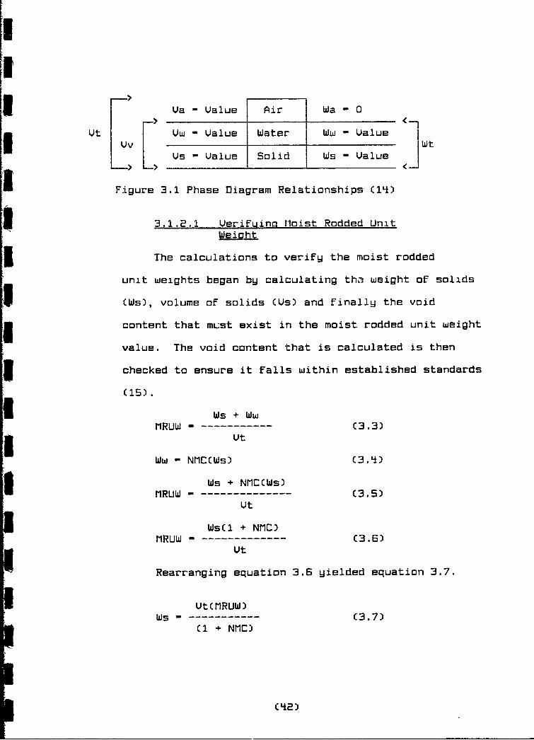
Figure 3.1 Phase Diagram Relationships (14)
3.1.2.1 Uerifuinq Moist Rodded UnitWeight
The calculations to verify the moist rodded
unit weights began by calculating tha weight of solids
(Ws), volume of solids (Us) and finally the void
content that must exist in the moist rodded unit weight
value. The void content that is calculated is then
checked to ensure it falls within established standards
(15).
Ws + WwMRUW - (3.3)I Vt
Ww - NMCCWs) C3.4)
Ws + NMC(Ws)MRUW - --------------- (3.5)
Ut
Ws(I + NMC)MRUW - -------------- (3.6)
Ut
Rearranging equation 3.6 yielded equation 3.7.
Vt(MRUW)Ws - (3.7)
C1 + NMC)
C(2)

III• Utilizing equation 3.7 with an assumed total volume
(Ut) of 1 cf, the Fine aggregate calculation was as
I follows.
Assumed: Ut - 1.00 cf
Given: NMCFA - .90• (16)
S~MRUW - 85.75 pcf
1.00 cfC85.75 pcf)WsFA ------------------
(I + .029)
WsFA - 83.33 lbs
Similarly the weight of solids for the coarse
aggregate (WsCA) equaled 89.00 lbs. Continuing on with
the fine aggregate brings on the volume of solid
5 calculation CUsFa). Equation 3.8 details the saturated
surface dry specific gravity relationship to the volume
I of solids (Us).
Wabw + Ws Ws(l + Abs)SSDSG - ---------------- --------------- (3.8)
Us * Gamma W Us * Gamma W
3 Rearranging equation 3.8 yields equation 3.9 which
was used to calculate the volume of solids.
I WsC1 + Abe)Us - (3.9)
SSDSG * GammaW
83.33 lbs(1 + 0.007)LUsFA ------------------------------------IsF 2.65(62.4 pcf)
UsFA - 0.51 cf
3 Similarly, the volume of solids for the coarse
3 aggregate CUsCA) equals 0.65 cf.
5 C *3)

I
Calculating the volume of the voids for both
aggregates is done by equation 3.10.
V v - Ot - Us (3.10)
Therefore the volume of voids calculation for the
fine aggregate was as follows.
VvFA - 1 - O.S1 - O.49 cf
Similarly, the volume of voids for, the coarse
aggregate equaled 0.35 cf. ThF void content values
CVvFA & UvCA) fell within expected ranges of 30 - 4S%
3for coarse aggregates and 40 - S0% for fine aggregates
(17).
1 3.1.2.2 Moist Rodded Unit Weiaht Ranaes
3 Working backwards through equations (3.10,
3.9 and 3.7) at the void ratio ranges of 30 - 35% for
the coarse aggregates and 40 - 50% for the fine
aggregates, yields moist rodded unit weight ranges of
,1 98.0 - 77.0 pcf for the coarse aggregate and
3 101.q 8'.5 pcf for the fine aggregate.
3.1.2.3 Void Ratios
3 The void ratios Ce) were calculated using
equation (3.11).
e - (3.11)Us
The values calculated for the fine and coarse
* aggregates are listed below.
Void Ratio (FA) - 0.97
Void Ratio (CA) - 0.53
I (44)

I3.1.2.4 Aggregate Parameter Rances
The ranges obtained from the Florida Mining
g Company (18) for absorption and the fineness modulus
are listed below in Table 3.4.
Table 3.4 Aggregate Parameter Ranges
1 Aggregates Fine CoarseHigh Low High Low
5 Absorption, % 0.71% O.69% 5.82% 5.60%
Fineness Modulus 2.4 2.0
5 3.2 Proportioning of Mix Design
3.2.1 Calculating Proportions bu Absolute3, Volume in Mix
The mix design follows the Maximum Density Approach set
I forth in the ACI Code (19).
Step (1)
I Set air-free volume of paste to air-free volume of
3 mortar CPv) equal to suitable value for interior mass mix in
accordance with ACI Code (20).
I Pv - 3B.0%
Step (2)
Select flyash/cement (F/C) and water/Ccement + Flyash)
(W/(C+F)) UOLUME ratios from ACI Code (21).
F/C - 0.0%
I Uolume W/CC+F) - 15i.0%
Step (3)
3 Select volume of coarse aggregate (Uca) by selection
5 ('45)

II
Ifrom ACI Code (22) by equating #57 approximately equal to
I 3/4" maximum size aggregatb (23).
3 Uca - 4S.O0
Step (q)
Calculate the volume of air-free mortar per cubic yard
Cum) assuming 2% entrapped air (Ua) (24) using equation
1 (3.12).
Va - 2.0%
Um - Cv * (I - Ua) - Uca (3.12)
I Um - 49.0%
where:
I Cv - the unit volume of concrete - Icy- 27 cF
Step (5)
Calculate the air-Free paste volume (Up), using the
selected paste volume ratio (Pv) of Step (1) and equation
5 (3.13).
Up - Um n Pv (3.13)
Up - 1B.6%
Step (6)
Determine the Fine aggregate volume CUfa) using
I equation (3.1q).
UFa - Um * (I - Pv) (3.11-)
Ufa - 30.4
Step (7)
I Determine the trial water volume (Uw) with equation
i 3.15.
Uw - Up * ECW/(C+F))/(I+W(C+F))] (3.15)
3 (Ls)
II
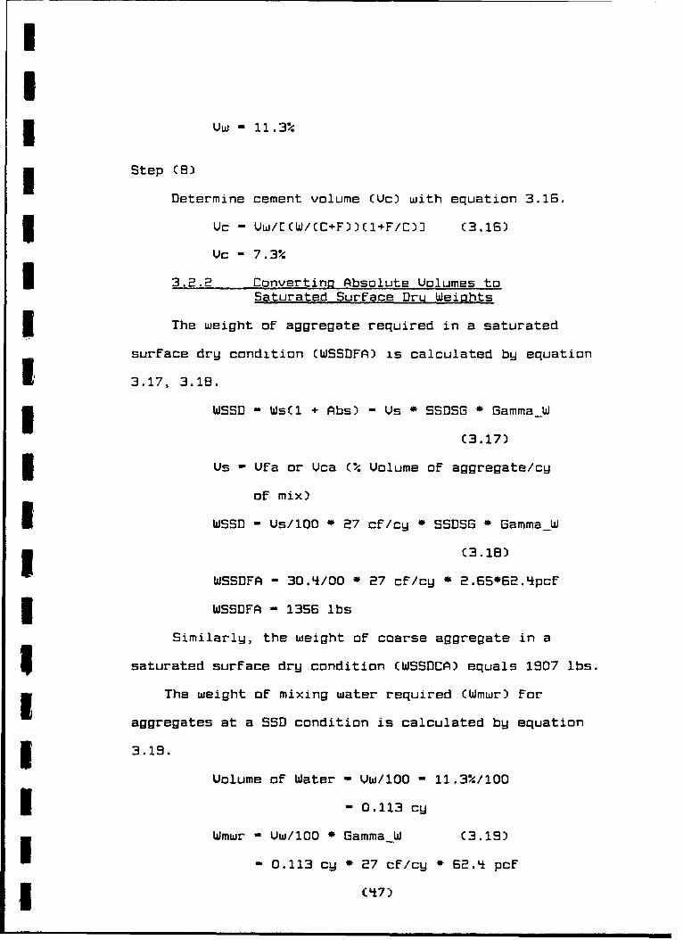
Uw - 11.3%
Step CB)
Determine cement volume (Uc) with equation 3.16.
3 Uc - Uw/ECW/CC+F))CI+F/C)3 C3.16)
Vc - 7.3%
U 3.2.2 Converting Absolute Uolumes toSaturated Surface Dru Weiahts
5 The weight of aggregate required in a saturated
surface dry condition CWSSDFA) is calculated by equation
3' 3.17, 3.18.
3 WSSD - WsCl + Abs) - Us * SSDSG * GammaW
C3.17)
Us - Ufa or Uca (% Uolume of aggregate/cy
of mix)
IWSSD - Us/IO0 * 27 cf/cy * SSDSG * Gamma_W
3 C3.18)
WSSDFA - 30.4/00 * 27 cf/cy * 2.65*62.qpcf
5 WSSDFA - 1356 lbs
Similarly, the weight of coarse aggregate in a
3 saturated surface dry condition CWSSDCA) equals 1907 lbs.
5 The weight of mixing water required CWmwr) for
aggregates at a SSD condition is calculated by equation
5 3.19.
Volume of Water - Vw/100 - 11.3%/100
I - 0.113 cy
Wmwr - Uw/100 * GammaW C3.19)
- 0.113 cy * 27 cf/cy * 62.4 pcF
(47)
II
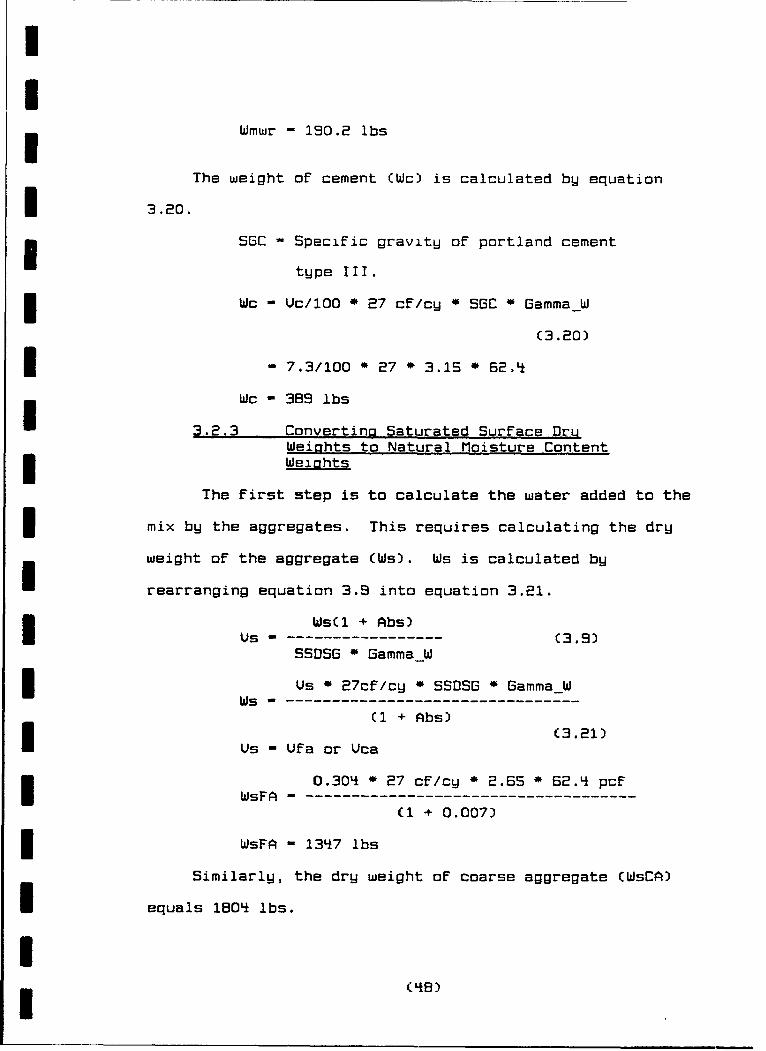
Wmwr - 190.2 lbs
The weight of cement CWc) is calculated by equation
I 3.20.
SGC Specific gravity of portland cement
type Ill.
Wc - Uc/iO0 0 27 cf/cy * SGC * Gamma_W
(3.20)
m 7.3/100 * 27 * 3.15 * 62.4
Wc - 3B9 lbs
3.2.3 Converting Saturated Surface DruWeights to Natural Moisture ContentWeichts
The first step is to calculate the water added to the
mix by the aggregates. This requires calculating the dry
weight of the aggregate CWs). Ws is calculated by
rearranging equation 3.9 into equation 3.21.
Us WsCl + Abs)Us --------------------------------- 3.9)
SSDSG * Gamma W
I s Us 0 27cf/cy * SSDSG * Gamma_WWs - - - - - - - - - - - - - - - - -
C1 + Abs)
Us - Ufa or Uca
0.304 * 27 cf/cy * 2.65 * 62.4 pcfWsFA --------------------------------------
(1 + 0.007)
WsFA - 1347 lbs
Similarly, the dry weight of coarse aggregate CWsCA)
I equals 1BO lbs.
(Lis)

II
The weight of mixing water contributed by aggregates
I CWmwca) is calculated by equation 3.22.
Wmwca - Wsi CNMCi -- Absi) (3.22)
Coarse:
1804 lbs * C0.027 - 0.057) -- 5L.3 lbs
Fine Agg:
I 1347 lbs * (0.029 - 0.007) 29.6 lbs
Wmwca -2q.7 lbs
The weight of adjusted mixing water required CWamwr) is
calculated by equation 3.23.
Wamwr - Wmwr - Wmwca C3.23)
I3W 190.2 lbs - C-24.7 lbs)
- 214.9 lbs
The weight of aggregates at natural moisture content
CWNMC) is calculated by equation 3.24.
Ws * (1 + NMC) - WNMC C3.24)
Coarse Agg CWNMCCA)
1804 lbs * 1.027 - 1853 lbs
Fine Agg CWNMCFA)
1347 lbs * 1.029 - 1386 lbs
The weight of portland cement emains the same when
going from SSD conditions to NMC conditions. Table 3.5 lists
weights and weight percentages of ingredients after moisture
adjustment at NMC. These are the amounts actually put in
3I place per cubic yard of mix. Moisture adjustment means the
(LIS)

amounts are adjusted for moisture pre-exsting or lacking in
the aggregates. The relationship between SSD weights
and NMC weights can be seen as the numbers are listed side
by side.
Table 3.S Actual Mix Design Summary (I Cy)
Theoretical ActualWeight Weight Weight%L SSD @ NMC @ NMC
Slump Cinches) 0.0 in 0.0 in N/A
Air Content % 2% 2% N/A
Water 180.2 lb 21q.9 lb 5.6%
Cement 388.0 lb 388.0 lb 10.1%
Coarse Aggregate 1807 lb 1853 lb 48.2%
Fine Aggregate 1356 lb 1386 lb 36.1%
Totals 38q3 lb 3843 lb 100.0%
Unit Weight iq2.3 pcf 142.3 pcf N/A
Table 3.6 lists the absolute volumes, SSD weights
CWSSD), Dry weights CWs), weight percentages, and dry
volumes (Us). Table 3.6 is provided For convenient
referencing.
(50)

I
H Table 3.6 Volumes and Weights of Ingredients.
I Absolute WSSD Ws (DRY) DRY Us
Uolumes Weights Weights Weight % ''.lCcF)
I Water - 11.3% 190.2 302.6 7.9% 3.0
Cement - 7.3% 389.0 389.0 10.1% 2.0
Coarse - i9.0% 1807.0 1804.0 46.9% 13.2
Air - 2.0% 0.0 0.0 0.0% 0.5
Fine - 30.4% 1356.4 1347.0 35.1% 8.2
Sums - 100.0% 3842.7 38k2.7 1i2.3 27.0a a
Sums equal, (water shifts)
I 3.2.4 Calculatino the Water/Cement (W/L
Ratio and Moisture Content of Mix
The water to cement ratio CW/C) is calculated by
equation 3.25.
W/C - WSSD/Wc (3.25)
W/C - 180.2 lbs/389.0 lbs
W/C - 8.89%
The overall moisture content of the mix should be
approximately 5 (+/- .3%) for the mix to ensure adequate
stiffness. That translates to 180 to 200 lbs of mixing
water for a mix design with unit weight from 140 - 14S pcf
(25).
III
i C51)
II
The moisture content of the mix (ICIM) is calculated bW
equation (3.22).
Gamma TM - Unit weight of mix - 142.3 pcf
I MCM - WSSD/C27 * Gamma TM) (3.22)
IIMCM - 190.2 lbs/(27 * 142.3)
MCM - 4.95%
IIIIIIIIIIIII
I C 52)

I
CHAPTER 4I InouiLAYER THICKNESS CALCULATION
.1Introduction
5 This chapters illustrates the procedure for converting
weights to pre-mix volumes which takes into account the
3 bulking of materials that are in a partially saturated
condition. This is required since material in the field
I will very rarely be oven-dt-y nor 100% saturated. The
determination of -riz general shape of the crater to be
repaired is discussed followed by the conversion from
pre-mix volumes tc layer thicknesses.
It is very important at this point tn undestand
I how the materials will be handled to create the concrete mi:"
I that forms the slab. The coarse aggregate required will
first be placed upon the ground as a homogeneous layer. The
I cement powder bags will then be placed, opened, and emptied.
The cement will then be spread forming a thin !ayer on top
I of the coarse aggregate. The sand will then be placed on
top OF the cement layer forming a homogeneous sand layer.
The layers will then be mixed using a large rotor tiller
I such as is commonly used in soil stabilization. For more
detailed construction information, refer back to Chapter two
I of this report.
The discussion of the type of crater includes the
discussion of the equivalent hole concept C26). The
equivalent hole concept involves all of slab material
(aggregates and cement) required for the crater to be placed
in layers that do not completely fill the crater or are
I (53)
outside of the crater. The dimensions of the layers can
vary from the dimensions of the actual crater, as long as
the total volume of material in the layers Ci.e. equivalent
hole) equals the volume of material required to make the
slab in the crater. The procedure is detailed below to
provide more clarity about this concept.
The equivalent hole concept begins by determining the
volume of actual crater to be filled. The depth of the
crater to be filled with concrete was set to 10 inches.
Therefore, only the top surface area of the crater will
affect the volume calculation. ince the volume of material
for the actual crater is calculated, it is used to calculate
dimensions of the equivalent hole. Two dimensions are
arbitrarily set, the third dimension is then calculated so
that the equivalent hole volume equals the actual crater
volume. For example, if the equivalent hole depth is
arbitrarily set at 6 ins and the equivalent hole width is
arbitrarily set at 5 ft., then the equivalent hole length is
calculated to allow the equivalent hole volume to equal the
actual crater volume. The material will have to be moved
into place in the actual crater by motor graders and/or
front end loaders.
4.2 Convertina NMC Weight Proportions to Pre-mix
Uolumes
The aggregates will be proportioned in the field based
on pre-mix volumes. The moist rodded unit weights CMRUW)
were obtained using the aggregates at their NMC. Having the
C54)
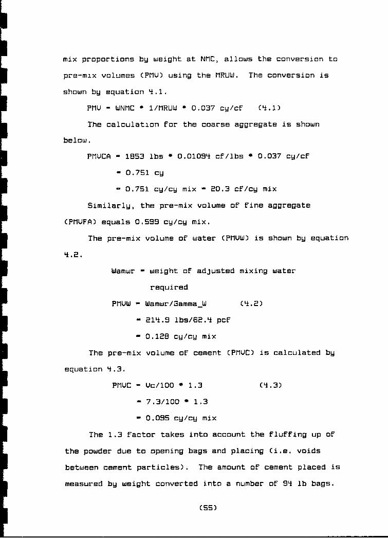
mix proportions by weight at NMC, allows the conversion to
pre-mix volumes (PMU) using the MRUW. The conversion is
shown by equation .1i.
PMU - WNMC * I/MRUW * 0.037 cy/cf (-i.1)
The calculation for the coarse aggregate is shown
below.
PMUCA - 1853 lbs * 0.01089 cf/lbs * 0.037 cy/cf
= 0.751 cy
- 0.751 cy/cy mix - 20.3 cf/cy mix
Similarly, the pre-mix volume of fine aggregate
(PMUFA) equals 0.59S cy/cy mix.
The pre-mix volume of water (PMUW) is shown by equation
Wamwr weight of adjusted mixing water
required
PMVW - Wamwr/GammaW N'.2)
- 21q.9 lbs/62.q pcf
- 0.128 cy/cy mix
The pre-mix volume of cement CPMUC) is calculated by
equation '.3.
PMUC - Uc/lOO * 1.3 C4.3)
- 7.3/100 * 1.3
- 0.095 cy/cy mix
The 1.3 Factor takes into account the fluffing up of
the powder due to opening bags and placing Ci.e. voids
between cement particles). The amount of cement placed is
measured by weight converted into a number of 94 lb bags.
C55)

II
The pre-mix volume of cement is only required to allow an
3 accurate measure of the combined height of the fine, coarse,
and cement layers.
I '*.3 Conv3rtiny Pre-mix Uolumes to Lauer Thicknesses
3 L.3.1 Calculating Crater Tupe and Size
The first requirement is to identify the general shape
3 of the crater. Most craters will fall into a circular or
rectangular shape. A section is devoted to irregular crater
I shapes. The slab depth is independent of the crater size.
The slab depth may be set to the existing slab depth plus
one or two inches to provide a safety margin against running
3 short of material.
4.3.1.1 Circular Crater Parameters
I For a circular crater with a surrounding slab
depth of 8 inches, the replacement slab is set at 10
inches as detailed in the example set of parameters
3 below in Table 4.1 for a circular crater.
3 Table q.1 Circular Crater Parameters
Slab Depth - 10 in
Diameter - 40 ft
3 rea - 12S7 SF
Slab Uolume - 38.8 Cy
I The slab volume can be converted to an equivalent
3 hole that can be placed within the crater. See Figure
C4.1) for an illustration. The water application will
I be discussed in detail in a later chapter, however, for
I (C56)

now it is essential to know whether the water spray bar
width can be adjusted or not. If the water spray bar
width cannot be adjusted then the equivalent width of
the crater should be set as some multiple of the
watertruck spray bar width. This will prevent
overlapping water during the water application phase.
Therefore, assuming a spray bar width of 10 i't, the
slab width could be set at 20 ft. IF the sprzj bar
width is adjustable, then the equivalent width should
be set as some multiple of the optimum width For
mixing by the mixer. The optimum width for the mixer
is the largest width the mixer can thoroughly mix on
one pass.
Since the crater is circular, the equivalent
length can be set as the diameter realizing that the
length will slightly shorter on sides away From the
center (see Figure q.1). The minimum of one inch of
extra slab thickness provides for at least 10% extra
material (I inch/S inches - 11%, 1 inch/B inches -
12.5%) which will ensure enough material is placed to
compensate For this slight shortening. Obviously, the
extra two inches selected will provide for even more
excess material. The slight shortening will typically
cause less than a 5% decrease in volume. See Figure
11.2 For more detail on the volume reduction due to
shortening.
(57)

W
Sli ght . .Shortening ,
S a I
W/2
L LD*WaterSpray ;j
aPath
WaterI V Spra Spray ,a : WItr
4• * Path3 a
* I
a a
a a
I I I
The Equivalent Width (W) is equal to two Spray Bar Widths
The Equivalent Length (L) is the Diameter
Figure 4.1. Circular Crater Equivalent Hole
(58)
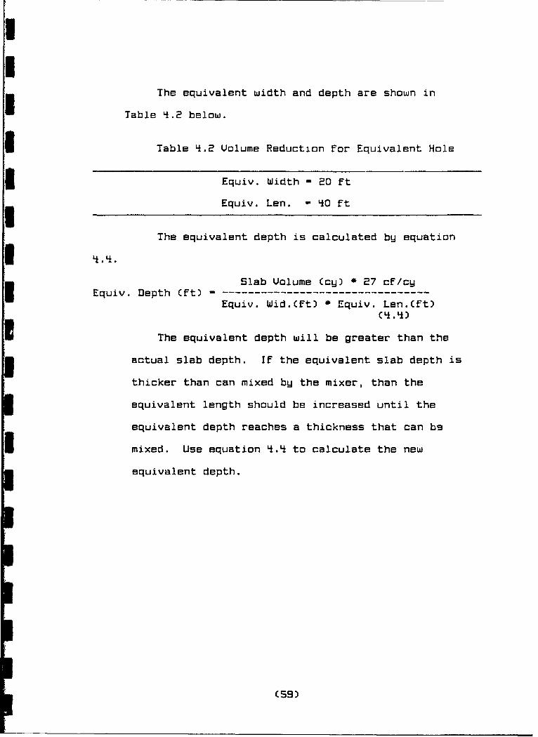
The equivalent width and depth are shown in
Table 4.2 below.
Table 4.2 Uolume Reduction for Equivalent Hole
Equiv. Width - 20 Ft
Equiv. Len. - 40 Ft
The equivalent depth is calculated by equation
Slab Volume (cy) * 27 cF/cWEquiv. Depth (ft) ---------------------------------
Equiv. Wid.Cft) * Equiv. Len.Cft)C( .4)
The equivalent depth will be greater than the
actual slab depth. If the equivalent slab depth is
thicker than can mixed by the mixer, than the
equivalent length should be increased until the
equivalent depth reaches a thickness that can bs
mixed. Use equation 4.4 to calculate the new
equivalent depth.
C 59)
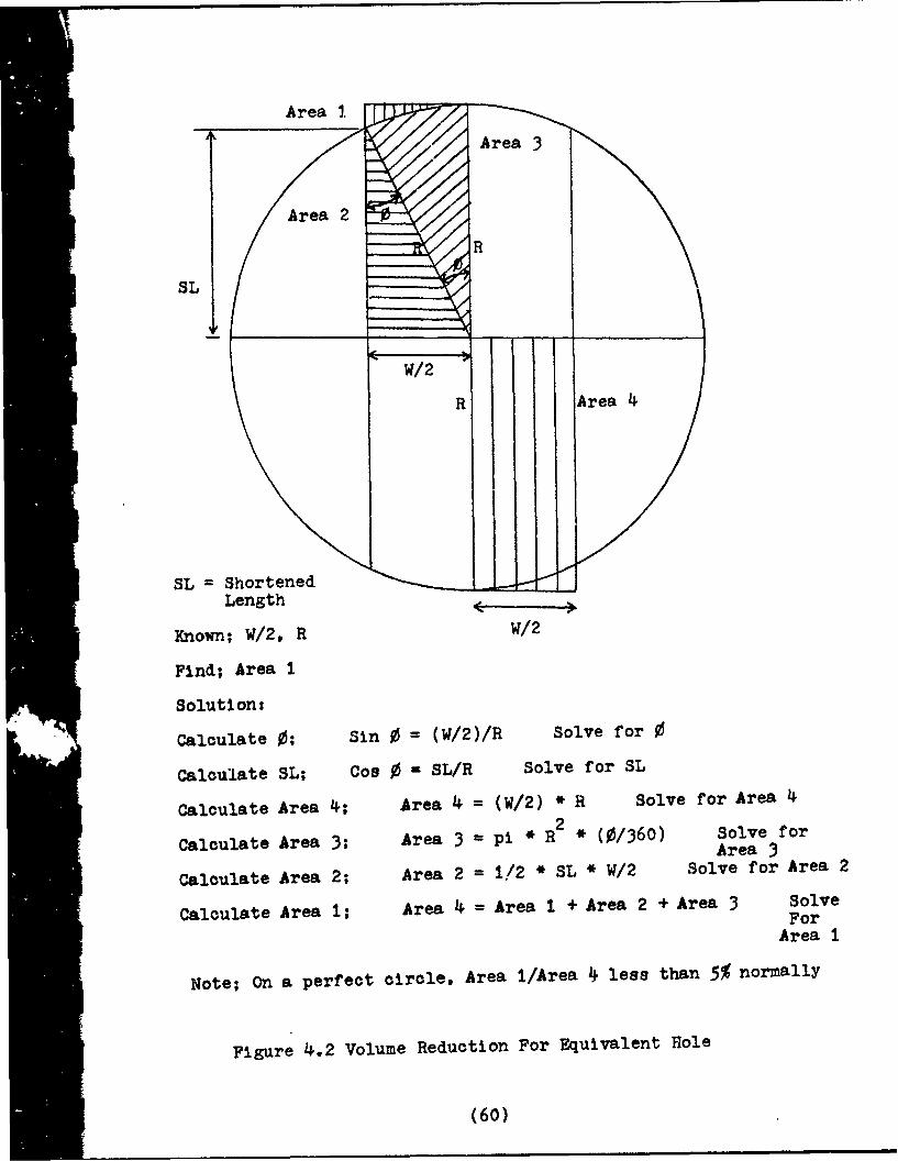
Area 1.Area I IArea 3
Area 2
R
SL
R Area 4
SL ShortenedLength •
Known; W/2, R W/2
Find; Area 1
Solution:
Calculate 0; Sin 0 = (W/2)/R Solve for
Calculate SL; Coo 0 = SL/R Solve for SL
Calculate Area 4; Area 4 = (W/2) * R Solve for Area 4
Calculate Area 3; Area 3 = pi * R2 * (0/360) Solve forArea 3
Calculate Area 2; Area 2 = 1/2 * SL * W/2 Solve for Area 2
Calculate Area 1; Area 4 = Area I + Area 2 + Area 3 SolveFor
Area I
Note; On a perfect circle, Area I/Area 4 less than 5% normally
Figure 4.2 Volume Reduction For Equivalent Hole
(60)

U
4.3.1.2 Rectangular Crater Parameters
A crater may come closer to resembling a
rectangular crater rather than a circular one.
In that event, the actual crater volume must be
3 calculated by breaking the crater area down into
smaller geometric shapes, calculating the areas of the
3 individual geometric shapes and summing the areas to
obtain the total crater area. The crater area can then
I be multiplied by
The 10 inch slab thickness to obtain the crater
volume.
* The crater volume can then be used to obtain
equivalent parameters. The use of an equivalent hole
3 can be accomplished by setting the equivalent width
3 equal to a multiple of the spray bar width. The
equivalent length can be set as the longest straight
I run through the hole. See Figure (4.3) for more detail
on the equivalent parameters. The equivalent depth can
I then be calculated using equation 4.4 above.
IIIII3 (61)

I. \
Water Spray Path
LI I
W
w i,a I
I 'I
W = Equivalent Width
L = Equivalent Length
Figure 4.3 Rectangular Crater Equivalent Hole
(62)

I.3.1.3 Irreaular Crater Parameters
If the crater is very irregular in shape, the
crater volume can still be calculated by breaking down
the crater into smaller geometric shapes. The
equivalent hole concept can then be used to determine
the dimensions of an equivalent hole. If placement of
the layers within the hole is difficult, then the
material may be placed in layers in an equivalent hole
outside of the actual crater.
1.3.1.4 External Equivalent Hole
Parameters
The field test conducted to test this rapid runway
repair method made use of the external equivalent hole
concept discussed in this section. The use of an
equivalent hole completely outside of the crater has
benefits and disadvantages over placing the material
directly in the hole.
A key difference between this method and regular
soil stabilization is that in normal soil stabilization
operations the mixer can only reach down to a maximum
depth of between 6 - 12 inches before mixing becomes
poor. The equivalent hole concept involves all of the
material being laid above ground on existing pavement.
Thick layers would be screeded off by the tractor
underbelly as the tractor towed the mixer behind it.
The screeding off should be limited to 2 - 3 inches or
else the tractor may experience difficulty traveling
over the material. The potential difficulties being
C63)

material falling into the engine compartment through
the Front grill of the tractor and uplift by material
being Forced underneath the tractor causing the tractor
to lose traction. Therefore, the combined layer
thicknesses before mixing should only be 2 - 3 inches
above minimum ground clearance of the tractor towing
the mixer. Th minimum ground clearance is usually
approximately 12 inches (27). By placing the material
outside of the hole and onto the existing pavement, the
use of a level bottom surface canbe taken advantage of
to measure the layer heights.
The principal disadvantage is that the material
must be moved farther to get it into the crater.
Further discussion on advantages and disadvantages of
the equivalent hole will be discussed in later
chapters.
The sequence of steps is the same as For
determining an equivalent hole within a crater. The
actual crater volume is deterined based on the actual
crater's dimensions.
The field test conducted to test this runway
repair method used this external equivalent hole
concept. The actual test crater was a 9 ft * 30 ft * 8
inch rectangular crater. The depth was increased by 2
inches to ensure enough material and provide for some
extra material to Fil small extraneous holes nearby
the test hole.
C 6'-

Therefore the actual crater dimensions for the
test were set at 9 ft * 30 ft * 10 inches yielding an
actual crater volume of 8.33 cy.
The water spreading width could easily be
adjusted to any width thereby eliminating the need to
set the equivalent width as a multiple of the water
spray bar width. Therefore, the equivalent width was
set based on the maximum width the mixer could
thoroughly mix. The maximum width was determined to be
5 ft to ensure excellent mixing of the aagregate and
cement layers. The depth was arbitraril,'4 set at 6
inches. Therefore, by switching sides of the
equivalent depth and length terms in equation (4.4),
the equivalent length was calculated to be 90 ft.
Table 4.3 below summarizes the actual and equivalent
parameters of the test hole.
Table 4.3 Actual and Equivalent Parameters ofTestHole
Actual Equivalent
Depth 10 in 6 in
Width 9 ft 5 ft
Length 30 ft 90 ft
Uolume 8.3 cy 8.3 cy
Once the actual volume of the crater was
determined, the total quantities of material required
could be calculated by multiplying the values required
(65)

Ifor 1 cy of mix by the total volume of 8.3 cW.
UI Therefore the values of Table 3.6 are reproduced and
increased by 8.3 to show a summary of total material
I required by weight to fill the testhole.
Table q.4 Actual Mix Design Summary Ci cy & 8.3Cy)
Actual ActualWeight Weight
@ NMC @ NMC(C cy) (8.3 cy)
Slump (inches) 0.0 in
Air Content % 2%
Water 214.8 lb 1791 lb
Cement 389.0 lb 3242 lb
Coarse Aggregate 1853 lb 15,q42 lb
Fine Aggregate 1386 lb 11,550 lb
Totals 3843 lb 32,025 lb
Unit Weight 142.3 pcf 1'2.3 pcf
3I.3.2 Calculatina Pre-Nix Lauer Thicknesses
Once the dimensions of the crater to be filled
were determined, the layer thicknesses were
calculated. The layer thicknesses were based on the
equivalent dimensions. If equivalent dimensions had
not been calculated (i.e. no equivalent hole was used), then
the actual dimensions would have been used.
The steps for calculating layer thickness were as
follows:
1. The volume of I cy C27 cf) was divided by the
C66)

III equivalent depth, thereby determining the surface area
covered by 1 cy of mix. Equation q.5 below was used to
3 perform the calculation.
Area = 27 cf/Equivalent Depth 0 12 in/ft Ci.5)
I Using equation q.5 the area was calculated.
Area - 27 cf/6 inches * 12 inches/ft
Area - 54 BF
3 2. The pre-mix volume (PMU) was converted from cy to
cf, divided by the surface area and multiplied by 12
3 to obtain the pre-mix layer thickness CPILT) in inches.
Equation q.6 below was used to perform the calculation.
PMLT - PMU * 27 cf/cy * 1/Area * 12 in/ft (4.6)
5 Using equation 4.6, the pre-mix layer thickness for the
coarse aggregate (PILTCA) was as follows.
3 PMLTCA - 0.751 cy * 27 cf/cy * 1/54 SF * 12 in/ft
PMLTCA - .5 ins
Similarly the fine aggregate and cement powder
3 thicknesses were 3.6 ins and 0.6 ins respectively.
5.3.3 Angle of Repose
5 As discussed the material was laid down in homogeneous
layers and then blended together by a soil stabilizer.
I Since there was no containment along the sides, each layer
I formed a trapezoid. The grades of the sides of the
trapezoidal layers are commonly referred to as angles of
3repose in geotechnical engineering (28).
The angles of repose For the coarse aggregate and fine
I 2ggregate were measured based on techniques shown in Holtz
(67)

(28). Table 4.5 contains the angles of repose for the
aggregates.
Table 4.5 Angles of Repose
Material Angle
Coarse Aggregate 30 degrees
Fine Aggregate 39 degrees *
SHigh angle value due to bulking of moist sand.
4.3.4 Calculatina Angle of Repose Lauer
Thicknesses
When the equivalent dimensions were calculated from the
crater volume, the assumption was that the layers would form
a rectangular box. The key concept is that the bottom of
the bottom layer width equaled the equivalent width (i.e. at
0 inches height, the width equaled S ft), however, the layer
width decreased (i.e. width < 5 ft) as the layer height
increased (i.e. height > 0 inches, moving up the trapezoid).
Therefore, in order to maintain the same volume one of the
other dimensions must be increased. The length was
arbitrarily selected to remain constant, therefore, the
layers depths were increased.
Since the length was 90 ft and the width was only 5 ft,
the depth increase due to the trapezoidal sides was
considered significant. The depth increase due to the
trapezoidal ends was considered insignificant due to the
short end lengths which were over an order of magnitudE 35
than side lengths; 5 ft < SO ft < SOft.
(68)

The angle of repose layer thicknesses were calculated
in the order of coarse aggregate on bottom, cement, and then
fine aggregate on top. Figure (4.4) shows the order of
placement of aggregates.
/ Fine Aggregate \/\
/ Cement\/\
Coarse Aggregate
Figure (4.4)
The following terms are defined in Table q.6 for use
with angle of repose layer thickness equations.
Table B.6 Angle of Repose Uariable Definitions
CA - Coarse Aggregate
FA - Fine Aggregate
ARLT - Angle of Repose Layer Thickness
PMLT = Pre-Nix Layer Thickness
CraWidth - Equivalent Width
- Width of Bottom Layer
RedCraWid- Reduced Top of Coarse Layer Width
The basic relationship is that the assumed rectangular
volume must equal the actual trapezoidal volume as detailed
in equation 4.7.
CraWidth * PMLTCA CraWidth + RedCraWid ARLTCA---------------------------------------------------------- S----- 0--------
12 2 12
(4.7)
(BE)

II5 The following equations are provided to illustrate the
derivation to obtain the final quadratic equation for angle
I of repose layer thicknesses (ARLTs).
ARLTCARedCraWid - CraWidth - 2 T-------- -------- C k.8)
Tan(ARCA) * 12
3 Substituting equation C into the right half only of
equation -.7 For RedCraWid is detailed below.
I 2 * Crawidth - 2 * ARLTCAI(Tan(ARCA) * 12) ARLTCA
2 12
I• The above right half of equation 4.7 simplifies as
I shown below.
ARLTCA ARLTCAraWdth- ---------
12 TanCARCA) 12
I Combining the above simplified right half of equation
4.7 back with the left half yields the following.
5 CraWidth * PMLTCA CraWidth * ARLTCA CARLTCA)2
i 12 12 TanCARCA)*I1
Further simplification yields equation q.8 as a
quadratic expression detailed below.
- (ARLTCA)2-------------- + ARLTCA(CraWidth) - PMLTCA(Crawidth)TanCARCA) * 12
For the coarse aggregate the a, b, c terms are detailed
below in Table 1.7.
III C 70)
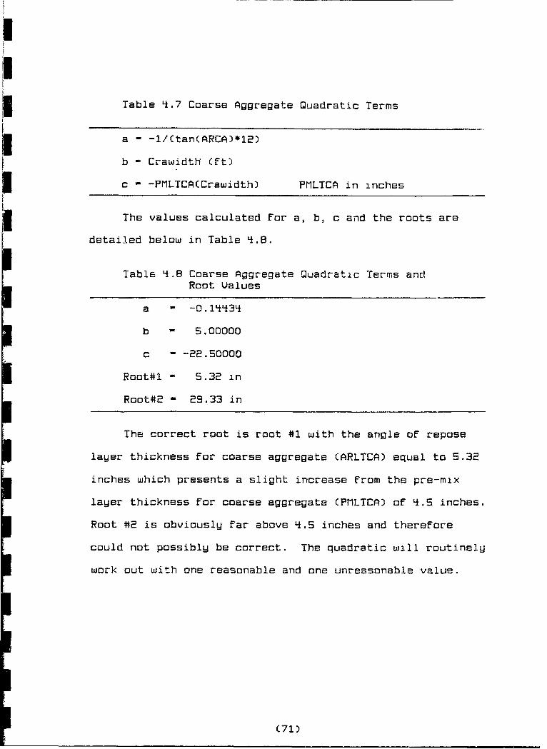
Table 4.7 Coarse Aggregate Quadratic Terms
a - -I/Ctan(ARCA)*12)
b - CrawidtH (ft)
c - -PMLTCA(Crawidth) PMLTCA in inches
The values calculated For a, b, c and the roots are
detailed below in Table q.8.
Table 4.B Coarse Aggregate Quadratic Terms and
Root Ualues
a -0.1434
b 5.00000
c - -22.50000
Root#1 - 5.32 in
Root#2 - 29.33 in
The correct root is root #1 with the angle of repose
layer thickness for coarse aggregate (ARLTCA) equal to 5.32
inches which presents a slight increase From the pre-mix
layer thickness for coarse aggregate CPMLTCA) of 4.5 inches.
Root #2 is obviously far above q.5 inches and therefore
could not possibly be correct. The quadratic will routinely
work out with one reasonable and one unreasonable value.
(71)
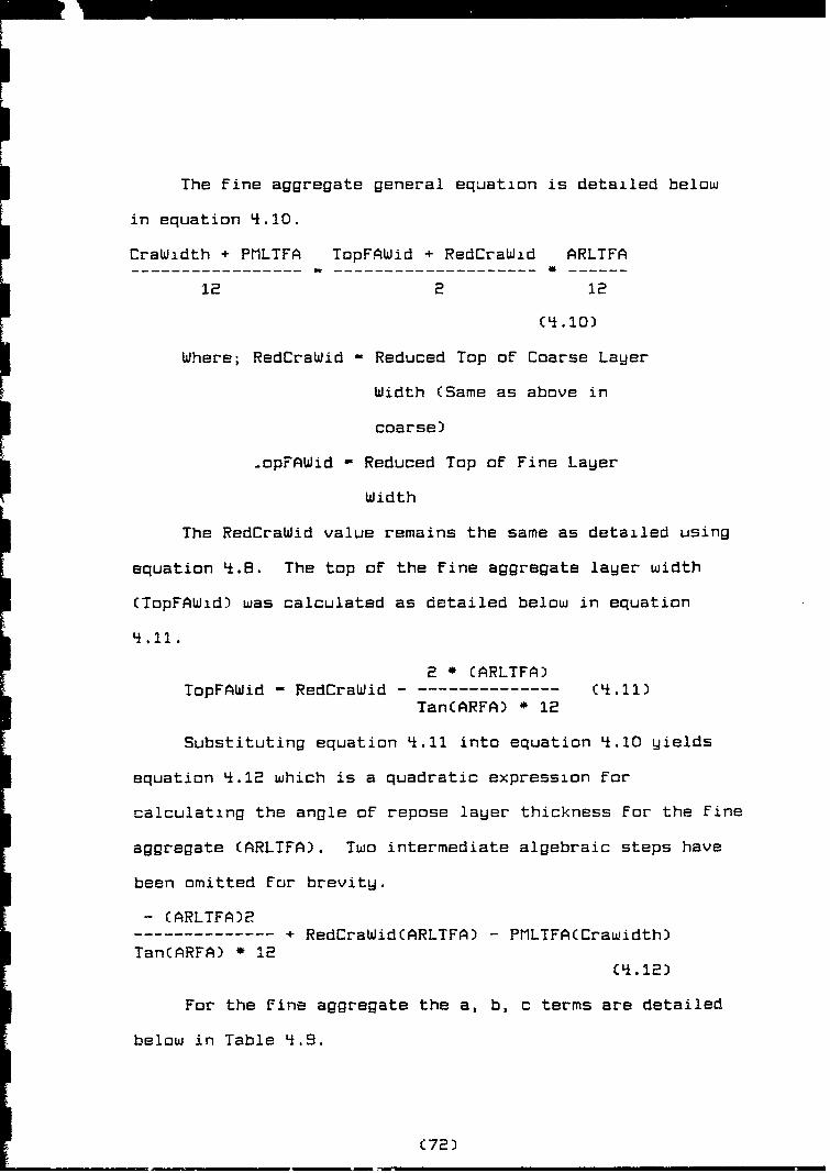
The fine aggregate general equation is detailed below
in equation 4.i0.
CraWidth + PMLTFA TopFAWid + RedCraWid ARLTFA
12 2 12
Lt.10)
Where; RedCraWid - Reduced Top oF Coarse Layer
Width (Same as above in
coarse)
.opFAWid - Reduced Top of Fine Layer
Width
The RedCraWid value remains the same as detailed using
equation 4.8. The top of the fine aggregate layer width
(TopFAWid) was calculated as detailed below in equation
4 ..11
2 * (ARLTFA)TopFAWid - RedCraWid --------------- (4.Ii)
Tan(ARFA) * 12
Substituting equation k.1i into equation 4.i0 yields
equation 4.12 which is a quadratic expression for
calculating the angle of repose layer thickness For the fine
aggregate CARLTFA). Two intermediate algebraic steps have
been omitted for brevity.
- (ARLTFA)2+ RedCraWid(ARLTFA) - PMLTFACCrawidth)
TanCARFA) * 12(CLt.12)
For the Fine aggregate the a, b, c terms are detailed
below in Table 4.9.
(72)

Table q.9 Fine Aggregate Ouadratic Terms
a - -I/CtanCARFA)*12)
b = RedCraWid = Top of coarse layer width (ft)
c - -PMLTFACCrawidth) PMLTFA in inches
The values calculated for a, b, c and the roots
are detailed below in Table 4.10.
C73)

II
Table q.10 Fine Aggregate Quadratic Terms andRoot Ualues
I a - -0.10291
b - 3.46829
c - -17.93980
Root #1 - 6.41 in
Root #2 - 27.29 inIThe correct root is root #1 with the angle of repose
layer thickness for the fine aggregate (CRLTFA) equal to
6.4I1 inches which presents an increase FV-om the pre-mix
I layer thickness for the fine aggregate (PMLTFA) of 3.6
inches. The narrowing of the base layer of coarse aggregate
underneath the fine aggregate magnifias the angle of repose
effect.
The angle of repose effect is neglected for the
I cement lagler due to the thinness of the cement lager at 0.6
inches. Table ..11 contains a listing of pre-mix volumes
CPMUs), pre-mix layer thicknesses and angle of repose layer
I thicknesses:
IIIII C7•

Table i.11 Layer Thicknesses
PMV PMLT ARLT(cy) (in) (in)
Coarse Aggregate * 0.751 1±.5 5.3
Cement 0.085 0.6 0.6
Fine Aggregate * 0.588 3.6 B.½
Water 0.128 0.6 0.8
Total Pre-Mix Thickness - 8.7 12.3
Water layer does not add to pre-mix thickness.
i.Li Calculating Spacing of Cement Bags
The following data is provided in Table q.12 for
caJcUlations in this section.
Table q.12 Cement Powder Data
One bag cement - 91 lbs (lbs cement/bag)
Cement/Cy mix - 388 lbs (lbs Cement/Cy mix)
Cy mix/one bag - 0.242 cy - 6.52q cf
Equiv. Depth - 0.500 ft
Type III high early strength cement was used which
comes in 8q lb bags. The amount of cement per cy of mix is
calculated in section 3.2. The cubic yards of mix (Cy mix)
per bag of cement was calculated by dividing the weight of
orE ',ag of cement (8$4 lbs) by the total weight of cement in
one cubic Ward of concrete (38 lbs). The equivalent depth
was determined to be 3 inches or 0.5 ft in section 4.3.1.q
as shown in Table q.3 of section q.3.1.q.
(75)
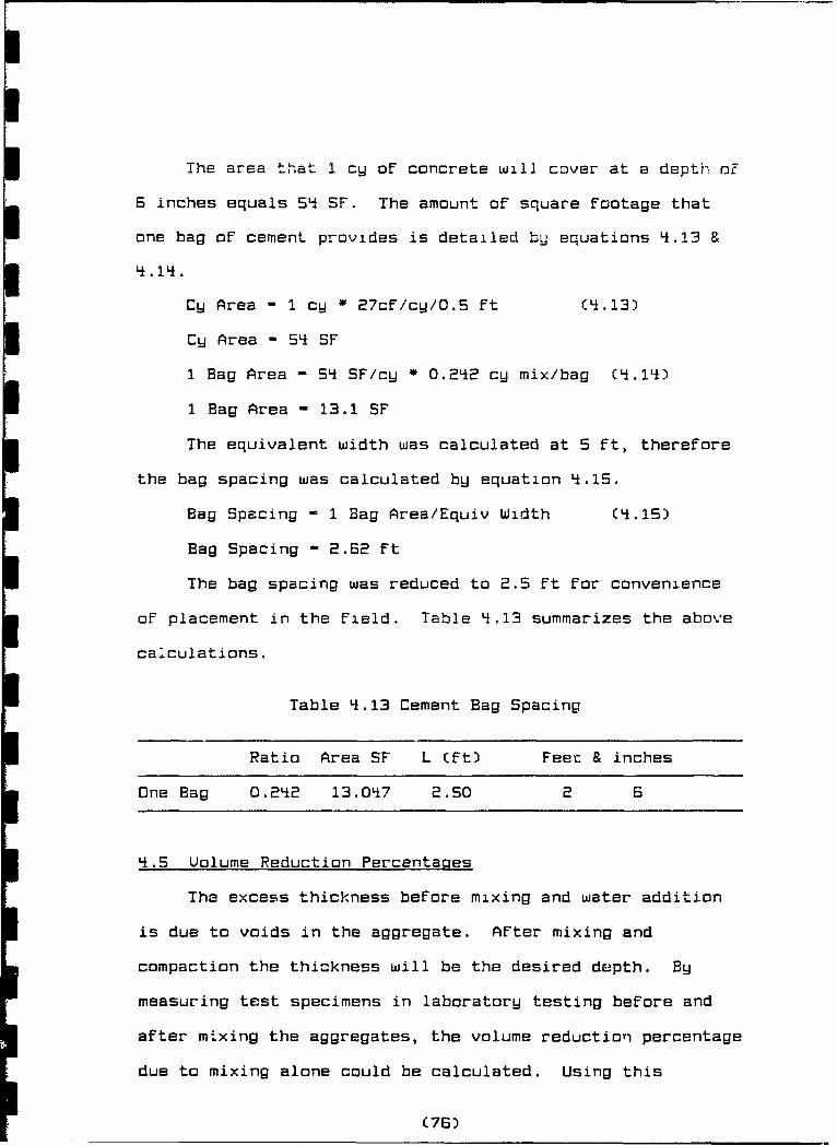
The area that 1 cy of concrete will cover at a depth oF
6 inches equals 54 SF. The amount of square footage that
one bag of cement provides is detailed bg equations 4.13 &
'1. i14.
Cy Area - 1 cy * 27cf/cW/O.5 ft (CI.13)
Cy Area - 54 SF
1 Bag Area - S SF/cy * 0.212 cy mix/bag (I.14)
1 Bag Area - 13.1 SF
The equivalent width was calculated at 5 ft, therefore
the bag spacing was calculated by equation q.15.
Bag Spacing = 1 Bag Area/Equiv Width (CL.1s)
Bag Spacing - 2.62 ft
The bag spacing was reduced to 2.5 ft for convenience
of placement in the field. Table 4.13 summarizes the above
calculations.
Table q.13 Cement Bag Spacing
Ratio Area SF L (ft) Feet & inches
One Bag 0.2'12 13.O017 2.50 2 6
q.5 Uolume Reduction Percentages
The excess thickness before mixing and water addition
is due to voids in the aggregate. After mixing and
compaction the thickness will be the desired dupth. Bu
measuring test specimens in laboratory testing before and
after mixing the aggregates, the volume reduction percentage
due to mixing alone could be calculated. Using this
(76)

II
reduction percentage, the reduction in the layers as the
mixer passes over them can be estimated. This layer
thickness reduction allows the mixer to work its way into
the layers during mixing. Table 4.11 lists the layer
3 thickness comparison for each material. An explanation of
the column headings is as follows:
3 1. The pre-mix thickness is the thickness of each layer
before mixing.
1 2. The reduced thickness is the layer thickness after
mixing of aggregates with water and vibration for 2 minutes.
3. The reduced fluff is the difference between the
previous two measurements for each material.
4. The absolute thickness is based on the absolute volumes
I within the concrete after the water is added and thoroughly
mixed in and the mix is compacted.
S. The absolute fluff is the difference between the
I absolute thicknesses and the pre-mix thicknesses. The
reduction percentages were calculated by the use of equation
I L4.16.
Red% - (Pre.Mix - After.Mix)/Pre.Mix N4.16)
The reduction percentage (Red%) for a test specimen
that measured 8.73 inches before mixing and 8.0 inches after
measuring equals 9.3%. Therefore, the aggregate and cement
3 layers were assumed to reduce equally by 9.3% as shown below
in Table 4.1q.
I(77)

II
I Table 4.lL Layer Thickness Comparison
Pre-Mix Red Red Absolute AbsoluteThick Thick FLUFF Thick FLUFF(in) (in) (in) (in) Cin)
Cement 0.572 0.519 0.053 0.440 0.132
I Coarse If.SOS LI.086 0. 419 2.940 1.565
Fine 3.592 3.258 0.334 1.823 1.769
Air 0.000 0.000 0.000 0.120 -0.120
Water 0.000 0.000 0.000 0.677 -0.677
Total 8.668 7.863 0.806 6.000 2.668
IIIIIIIIIUI
(78)
II
QUALITY UERIFICATION3 CHAPTER 5
5.1 Introduction
Quality verification involved testing the concrete mix
for strength at various intervals of time. The two major
variables were the method of mixing and the method of
3 compacting. There were two methods of mixing; laboratory
mixing and field mixing. Laboratory mixing consisted of
3 using a small mixing drum to thoroughly mix the materials.
Field mixing consisted of using soil stabilizing equipment
I to mix the material laid down in layers of coarse aggregate,
3 cement powder, and fine aggregate. There were two methods
of compaction; laboratorW compaction and field compaction.
3 Laboratory compaction consisted of using a compaction hammer
or a small sledge hammer to strike the mixed material
I contained in a test mold. Field compaction consisted of the
vibratory roller compacting material placed in the
test slab filling the test crater.
A third major variable that existed was the method of
measuring the quantity of materials put into the mix. The
3 two methods were by weighing and by pre-mix volumes. Test
specimens that were laboratory mixed had their materials
weighed by scale to measure input quantit3.es. Test
I specimens that were field mixed had their quantities
measured based on pre-mix volumes as discussed in section
I 'k.2. Therefore, laboratory mixing implies input quantities
measured by weight and field mixing implies input quantities
measured by pre-mix volume. For this reason only two
I C79)

I
variable combinations are discussed Cmixing and compaction)
with the third variable implied (measuring input
3 quantities).
The testing involved test specimens prepared under
three different combinations of the two major variables of
3 method of mixing and method of compaction. The first
combination was a concrete mix that was laboratory mixed
(drum mixer) and laboratory compacted (compaction hammer).
The second combination was field mixed (soil stabilizer) and
I laboratory compacted (small sledge hammer). The third
3 combination was field mixed and field compacted (vibratory
roller).
3 The results were analyzed by using simple linear
relationships. Although the linear relationships were not
I completely accurate, they provided valuable insight as to
basic compaction versus strength relationships at the
expense of some accuracy.
3 5.2 Settlement Tests
A settlement test was conducted only on the field mixed
I and compacted material. The settlement test was begun as
soon as the compaction activity was completed. The test
consisted of placing a 100 lb plate that was supported by q
3 steel rods that provided a contact of 1 square inch all
totaled. Figures 5.1 & 5.2 illustrate the plate placement
3I procedure. Therefore, the stress placed on the slab by the
1 steel plate was 100 psi. The stress was increased by
placing additional 100 lb plates to a maximum of q plates
3 (BO)

f or 2 4*00 psi stress. Figure S.3 snows the maximum stress
plate arrangement.
Fiur 5~. 1 lcmn fPaeLa
IFigure 5.1 PLoad eet Plate L100asi
I81

N!
I,
In
III
I iue53Fll oddLa PaeCIDpi
U|I' ' ••• ii i

The placement of the plates after compaction was
considered to be time 0. At time 0, settlements occurred as
detailed in Table 5.1.
Table 5.1 Settlements in Plate Load Test
Stress Rod 1 Rod 2 Rod 3 Rod q Average(psi) (in) (in) (in) (in) (in)
100 0.25 0.25 0.0 0.00 0.125
200 0.1 2.00 1.25 1.25 1.150
I0O0 1.75 1.50 1.75 1.50 1.625
At time +1 hour, the settlements were 0 inches at a qO0
psi stress.
5.3 Laboratorw Testing of Laboratoru Mixed andCompacted Test Specimens
The first combination of major variables was material
that was laboratory mixed and compacted. Tests on this first
variable combination were performed to establish the
strengths obtainable based on the mix design only (i.e.
eliminate mixing and compaction error). These tests were
performed on test specimens prepared by weighing the
portions of materials to eliminate proportioning errors.
The materials were then mixed using a small concrete drum
mixer to provide complete mixing. The mix was placed in
test specimen molds and then compacted with a CN-q15
Standard Compaction Hammer (5.5 lb * 12 inch drop) to obtain
a minimum of 95% compaction. Six 4 inch * 8 inch cylinders
and three 3 inch * 3 inch * 11 inch beams were prepared for
testing.
(83)

The preparation of the test specimens to test the mix
design was conducted as to eliminate all other possible
causes of error that could cause a weak mix to be developed.
3 Hence, the use of a mixing drum, scale, and compaction
hammer were required.
The cylinders were capped in accordance with ASTM C617
3 (Capping Cylinder Concrete Specimens). The compression
tests were performed in accordance with ASTM C39-86 (Test
U Method for Compressive Strength of Cylindrical Concrete
Specimens). The flexural strength tests were performed in
accordance with ASTM C7B-8i (Test Method for Flexural
3 Strength of Concrete). The tensile strength tests were
performed in accordance with ASTM Ci96-87 (Test Method for
I1 Splitting Tensile Strength of Cylindrical Concrete
Specimens).
The test specimens were tested for compressive,
3 flexural, and tensile strength at 24 hours and 8 days after
the mix preparation. The results of the compressive tests
3 had to be corrected due to the shortness of the samples.
ASTM C'k2-BS (Method of Obtaining and Testing Drilled Cores
I and Sawed Beams of Concrete) specifies that samples with a
I length to diameter ratio (L/d) below l.S9 must have
correction factors applied to reduce strengths obtained
3 (30). The stresses were calculated by dividing the load by
the area of the cylinder. Table 5.2 lists the cylinders
I along with the loads, areas, uncorrected stresses,
I C84)
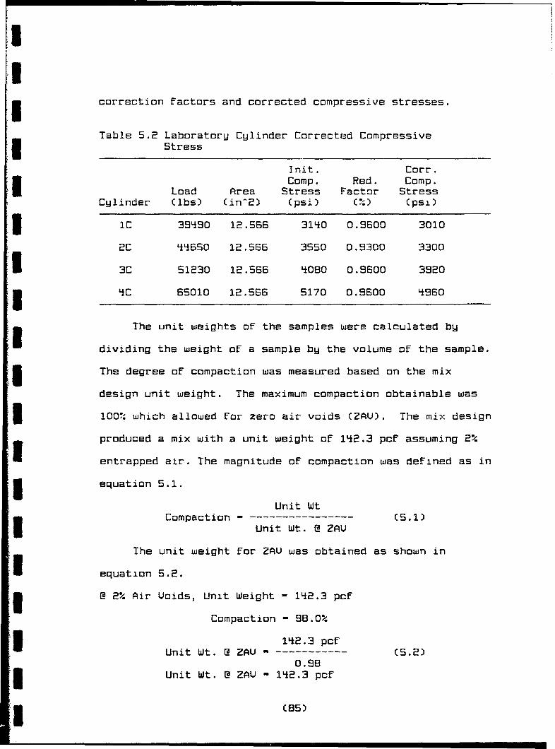
i correction Factors and corrected compressive stresses.
Table 5.2 Laboratory Cylinder Corrected Compressive3 Stress
Init. Corr.Comp. Red. Comp.
Load Area Stress Factor StressCylinder (ibs) (in^2) (psi) M%) (psi)
3 IC 39Li90 12.566 3140 0.9600 3010
2C ''si650 12.566 3550 0.9300 3300
I 3C 51230 12.566 '080 0.9600 3920
3 'C 65010 12.566 5170 0.9600 '*960
The unit weights of the samples were calculated by
dividing the weight of a sample by the volume of the sample.
I The degree of compaction was measured based on the mix
design unit weight. The maximum compaction obtainable was
3 100% which allowed for zero air voids (ZAU). The mix design
produced a mix with a unit weight of 142.3 pcF assuming 2%
entrapped air. The magnitude of compaction was defined as in
3 equation 5.1.
Unit WtCompaction ----------------- (5.1)
Unit Wt. @ ZAU
The unit weight for ZAU was obtained as shown in
I equation 5.2.
@ 2% Air Uoids, Unit Weight - iq2.3 pcf
Compaction - 98.0%
3 1'*2.3 pcFUnit Wt. @ ZAU - ------------ CS.2)
0.98Unit Wt. @ ZAU - 142.3 pcF
3 (85)
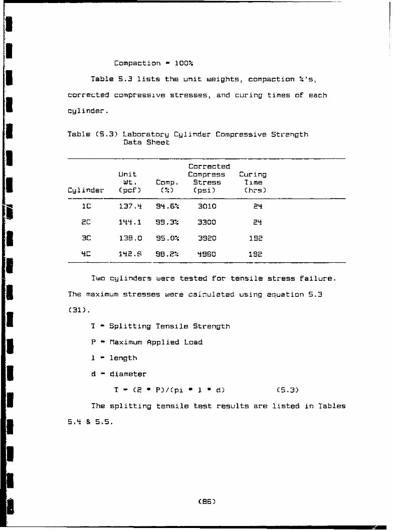
Compaction 100%
Table 5.3 lists the unit weights, compaction V's,
corrected compressive stresses, and curing times of each
cylinder.
Table (5.3) Laboratory Cylinder Compressive StrengthData Sheet
I CorrectedUnit Compress Curing
Wt. Comp. Stress TimeCuylinder (pcf) (%) (psi) (hrs)
5 IC 137. S9B*.6% 3010 24
2C I' ,.1 99.3% 3300 24
3C 138.0 95.0% 3920 192
LIC 0 Ii2.S 98.2% 4960 192
ITwo cylinders were tested For tensile stress failure.
The maximum stresses were cairulated using equation 5.3
(31).
C) T - Splitting Tensile Strength
P - Maximum Applied Load
1 - length
3 d - diameter
T ( 2 * P)/Cpi * 1 * d) (5.3)
The splitting tensile test results are listed in Tables
5.4 &5.5.
i (86)
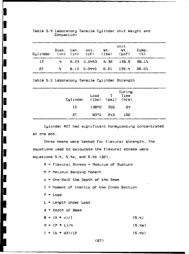
Table 5.4 Laboratory Tensile Cylinder Unit Weight andCompaction
UnitDiam. Len. LUol. Wt. wt. Comp.
Cylinder (in) (in) (cf) (Ibs) Cpcf) C%)
IT t 6.23 O.Ok53 6.32 139.5 96.1%
2T f 6.13 0.0445 6.21 139. L 96.0%
Table 5.5 Laboratory Tensile Cylinder Strength
CuringLoad T Time
Cylinder Clbs) (psi) (hrs)
iT 13B70 355 21f
2T 9370 2Li3 192
I Cylinder #2T had significant honeycombing concentrated
at one end.
Three beams were tested For flexural strength. The
equations used to calculate the Flexural stress were
equations 5.4, 5.qa, and 5.b (32).
R - Flexural Stress - Modulus of Rupture
M - Maximum Bending Moment
c - One-Half the Depth of the Beam
I - Moment of Inertia of the Cross Section
P - Load
L - Length Under Load
d - Depth of Beam
R - CM * c)/I (5.*L)
M (P * L/4I C5.4a)
I " Cb d3)/12 C5.4b)
(87)
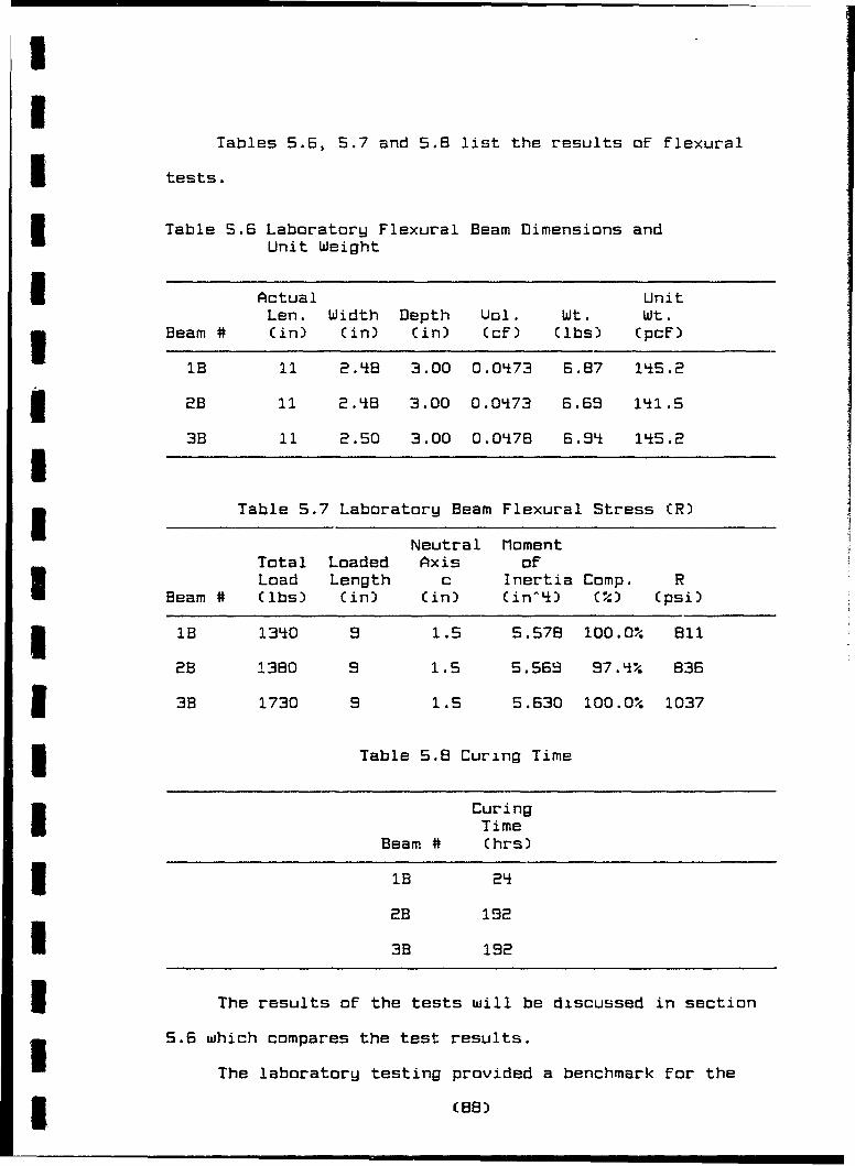
II
Tables 5.6, 5.7 and 5.8 list the results of flexural
I tests.
Table 5.6 Laboratory Flexural Beam Dimensions andUnit Weight
UActual UnitLen. Width Depth Uol. Wt. Wt.3Beam # (in) (in) (in) (cE) (lbs) CpcE)
1B 11 2.48 3.00 0.0q73 6.87 15S.2
32B 11 2.-8 3.00 O.0L73 6.68 1'*1.5
3B 11 2.50 3.00 0.0i78 6.89i 14I5.2
Table 5.7 Laboratory Beam Flexural Stress (R)
Neutral MomentTotal Loaded Axis ofLoad Length c Inertia Comp. R
Beam # (lbs) (in) (in) (in^') C%) (psi)
31B 13'*0 9 1.5 5.578 100.0% 811
2B 1380 9 1.5 5.569 97.4% 836
3B 1730 9 1.5 5.630 100.0% 1037
3 Table 5.8 Curing Time
CuringTime
Beam # (hrs)
11B 21f
2B 192
I3B 192
I The results of the tests will be discussed in section
5.6 which compares the test results.
The laboratory testing provided a benchmark for the
1 (B8)

judging the compressive strengths obtained in the field
test. The mix design detailed in section 3.2 was followed
to produce the laboratory test specimens.
5.4 Laboratory Testinp of Field Mixed and Laboratoru
Compacted Test Specimens
The second combination of field mixed and laboratory
compncted was performed to minimize compaction error and
isolate the effect of strengths by field mixing.
After completion of the mixing operation by the soil
stabilizer during the field test, samples were removed from
the mixed material and placed into cylinders. Figure S.i
shows the mixed material in place that the sample material
was taken from. The cylinders were placed on the vibratory
drum and vibrated for four minutes as shown in figure 5.5.
The cylinders were then compacted using a small sledge
hammer and a small tamper as shown in figure 5.6. Seven 6
inch * 12 inch cylinders were prepared For compression
tests. The flexural and tensile strengths were obtained by
using known Flexural and tensile strength relationships for
concrete (33). Figure 5.7 shows two of the sawcut cylinders.
Figure 5.8 shows the capping procedure being performed on a
cylinder in accordance with ASTM C617 (capping Cylinder
Concrete Specimens).
(89
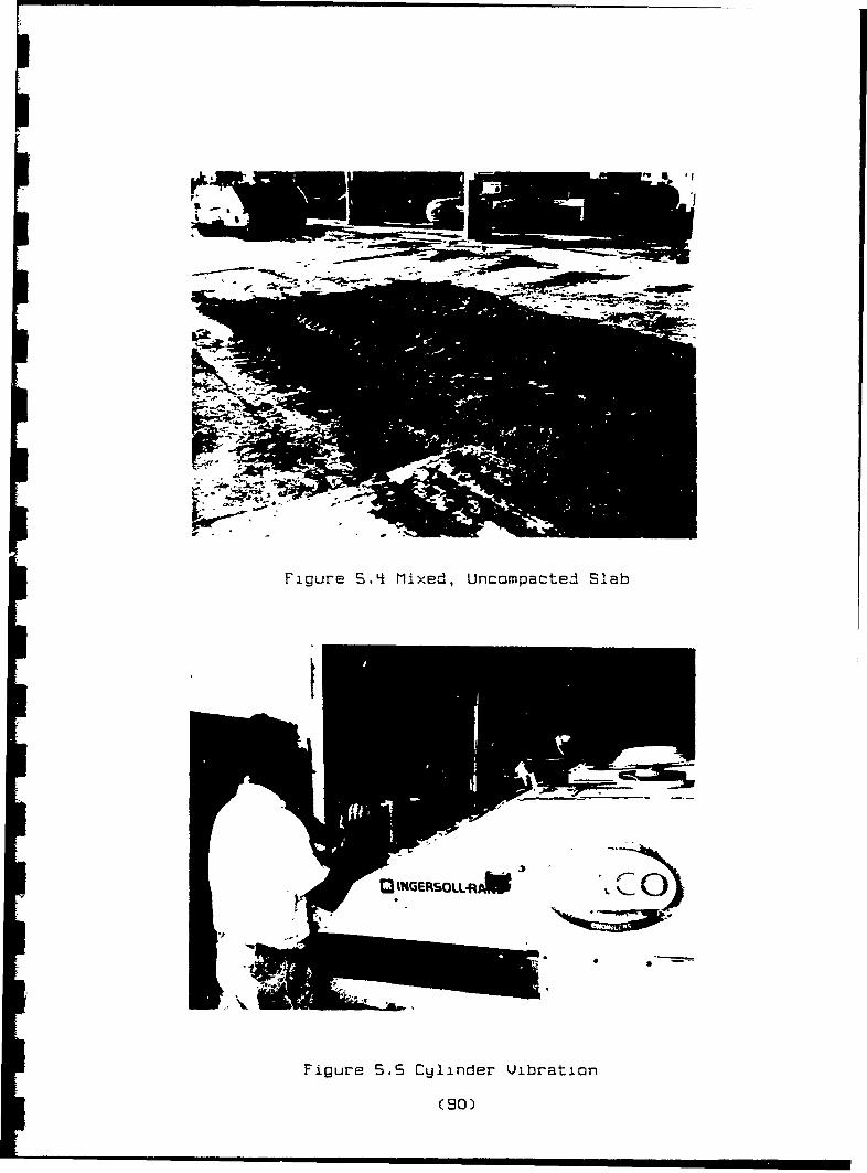
Figure S.q~ Mixed, Uncompactezi Slab
SINGEFRSOLL-R* ISi
Figure 5.5 Cylinder V~ibration
(90)
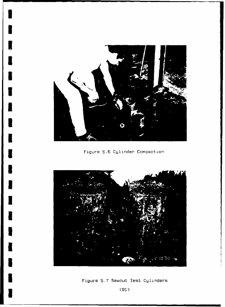
1IIIIIIII3 Figure 5.6 C�1inder Compection
IIIIIIII Figure 5.7 Sawcut Test Cylinders
3 (91)

IIIIIIIUI
Figure 5.8 Cylinder arid Cylinder- Capping Mold
IIIIIIII3 (92)
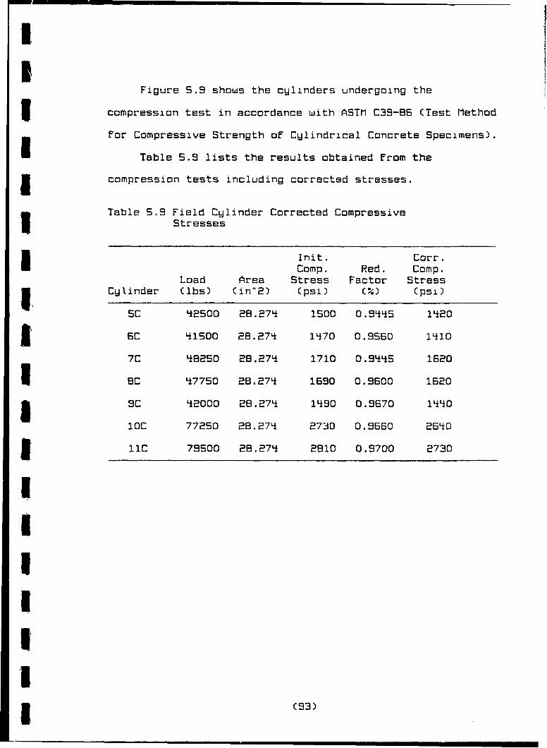
IFigure 5.9 shows the cylinders undergoing the
compression test in accordance with ASTM C39-86 (Test Method
for Compressive Strength of Cylindrical Concrete Specimens).
Table 5.9 lists the results obtained From the
5 compression tests including corrected stresses.
Table 5.9 Field Cylinder Corrected CompressiveStresses
Init. Corr.Comp. Red. Comp.Load Area Stress Factor Stress
I Cylinder (lbs) (in^2) (psi) (%) Cpsi)
SC q2500 28.27q 1500 0.9445 1420
6 6C 41500 28.27q 1'70 0.9560 1410
7C 482S0 28.2711 1710 0.9445 1620
BC 47750 28.27q 1690 0.9600 1620
9 9C q2000 28.274 1490 0.9670 iLHO
lOC 77250 28.271 i 2730 0.9660 26Li0
I 1IC 79500 28.274 2810 0.9700 2730
(IUIII1 (93)

Figure S.9 Compressive Test Performance
i (94)

IIg Table 5.10 lists the compaction percentages, corrected
stresses and curing times side by side.
Table 5.10 Field Cylinder Compressive Strength DataSheetI
CorrectedUnit Compress Curing
Wt. Comp. Stress TimeCylinder (pcf) M•) (psi) Chrs)
35C 141.7 97.6• 1420 14
6C 141.7 97.6% 14 10 1 LI
I 7C 141.1 97.2% 1620 1i
BC 1{0.5 96.85 1620 i4
IC 140.5 96.8% 1lfi0 2
i lOC 1q1.2 97.2% 26t0 24
IIC ILfO.1 96.5 2730 72
i The results of the tests will be discussed in section
I 5.6 which compares the test results.
5.5 Laboratoru Testina of Field Mixed and Compacted
Test Specimens
The field mixed and compacted samples were obtained the
3 day following the slab construction. The samples were
actually cored out of the slab using a coring machine.
Since the samples had to be Field mixed by the mixer and
3 field compacted by the vibratory roller, obtaining the core
samples was the only method of producing test specimens.
Six core samples were taken from different locations
throughout the slab. Appendix D lists the exact locations
I in the slab that the core samples were taken from. The
I (95)

flexural and tensile strengths were obtained by using known
Flexural and tensile strength relationships for concrete
(3•)
Table 5.11 lists the results obtained From the core
I samples.
5 Table S.11 Field Core Corrected Compressive Stresses
Init. Corr.Comp. Red. Comp.
Load Area Stress Factor StressI Core Cibs) Cin^2) (psi) (%) (psi)
12C 21400 6.026 3550 1.0000 3550
13C 10000 6.02 1660 1.0000 1660I4C 15000 6.026 2'*90 1.0000 2Si90
ISC 14'IOO 6.026 2390 1.0000 2390
i Table 5.12 lists compaction percentages side by side
with the corrected compressive stresses and curing time of
3 each sample.
I Table 5.12 Compressive Strength Data Sheet
CorrectedUnit Compress Curing
Wt. Comp. Stress TimeCore (pcf) M%) (psi) (hrs)
12C 141.3 97.3% 3550 72
13C 133.6 92.0% 1660 72
14IC 140.5 96.8% 2490 168
I 15C 138.6 95.5% 2390 168
The results of the tests will be discussed next in
section 5.6.
I C(96)

II
5.6 Comparison of Laboratory Mixed and Compacted,Field Mixed and Laboratoru Compacted, and FieldMixed and Compacted Test Specimens
The results of each combination tested are listed in
Table 5.13 below.
Table 5.13 Summary of All Actual Stresses
SPECIMEN COMPRESS FLEX TENSILE COMPACT'N TIME# (R) (T) (%) HIRS)
(psi) (psi) (psi)
IC 3010 9-. 6% 24
2C 3300 98.3% 2'i
3C 3920 95.0% 192
LiC '*960 98.2% 192
SC 1L120 97.6% I4
1 6C I410 97.6% ILf
7C 1620 97.2% iL
BC 1620 96.8% I4
9C 1440 96.8% 2'-
lOC 264 0 97.2% 2i
I IIC 2730 86.5% 72
12C 3550 97.3% 72
13C 1660 92.0% 72
I4IC 2490 96.8% 168
15C 2390 85.5% 168
1 IB Bl 100.0% 2I
2B 836 97. 4% 192
3B 1037 100.0% 192
IT 355 96.1% 2Lf
2T 243 96.0% 192
I (C97)

Since each sample could be tested for only one
type of stress (compressive, tensile, or flexural) known
relationships for compressive to flexural, compressive to
tensile, and tensile to flexural were used to obtain a set
of three stresses for each sample (35). The values of the
stress relationships used are listed in Table 5.1.
Table 5.1q Stress Relationships
Split Tensile/Compressive - 10.0%
Flexural/Compressive W 15.0%
Split Tensile/Flexural - 62.S%
Therefore, to obtain a flexural value for specimen iC,
the compressive strength (stress) value was multiplied by
the Flexural/Compressive ratio to obtain a Flexural value.
The laboratory mixed and compacted sample relationships of
flexural to compressive (approx. 26%) and tensile to
compressive (11%) exceed the relationships in Table S.14
Later calculations developed in this report are based on
compressive strengths. Therefore, the lower ratios in Table
5.11 are conservative since they will produce lower
compressive strengths from flexural and tensile strengths as
tabulated in Table 5.15.
(98)

II3 Table 5.15 Actual and Calculated Stress Values
SPECIMEN COMPRESS FLEX TENSILE COMPACT'N TIME# CR) (T) M%) CHRS)
Cpsi) (psi) (psi)
1 C0 3010 Lf52 301 S4. 6% 24
2C 3300 Lf 5 330 99.3% 24
3C 3920 588 382 95.O 192
qC -i96O 7LiLf L196 99.2% 192
5C 1h20 213 14 2 97.6% 146C 1'LtO 212 141 97.6% 1 -
7C0 1620 243 162 97.2% iL
IBC 1620 2'i3 162 96.8% iL
9C 1 LL0 216 1 L L 96.8% 2B
3 DC 26L50 396 265 97.2% 2Li
liC 2730 '-110 273 96.S% 72
12C 3550 533 355 97.3% 72
I 13C 1660 249 166 92.0% 72
V-ic 2490 37Lf 249 96.8% 168
15C 2390 359 239 95.5, 168
1B 5405 811 S07 100.0% 2O
2B 5576 836 523 97.4% 192
3B 691Li 1037 6SLI I00.0% 192
IT 35LI6 567 355 96.1% 2q
I 2T 2Li35 390 243 96.0% 192
II (99)
5.6.1 Compressive Strength UersusCompaction%
The relationship of compaction percentage versus
compressive strength was investigated.
Th laboratory mixed and compacted samples tested at 24
hours CIC, 2C, IB, IT) yielded substantial scatter of
compressive strengths. The results were processed through
linear regression to obtain a simplified linear
relationship. The linear relationship shows that the
strength increased as compaction increased. Figure 5.10
shows the points and linear relationship.
The laboratory mixed and compacted samples that were
tested at 8 days C3C, 4C, 2B, 3B, 2T) yielded a minimum of
scatter for compressive strengths. The results were
processed through linear regression to obtain a simplified
linear relationship. The linear relationship shows that the
strength increased as the compaction increased. Figure 5.11
shows the points and linear relationship.
C100)

* 0
0 z0
00C
I zM-J
> 0Il zoa-- en z
LLJ'
rz.
LlLil c
(1) 0
CLL 0
10 :-
(spuosnoi4_)(Isd) H.LON3ý1S 3AISSdJ~4O~
* (101)
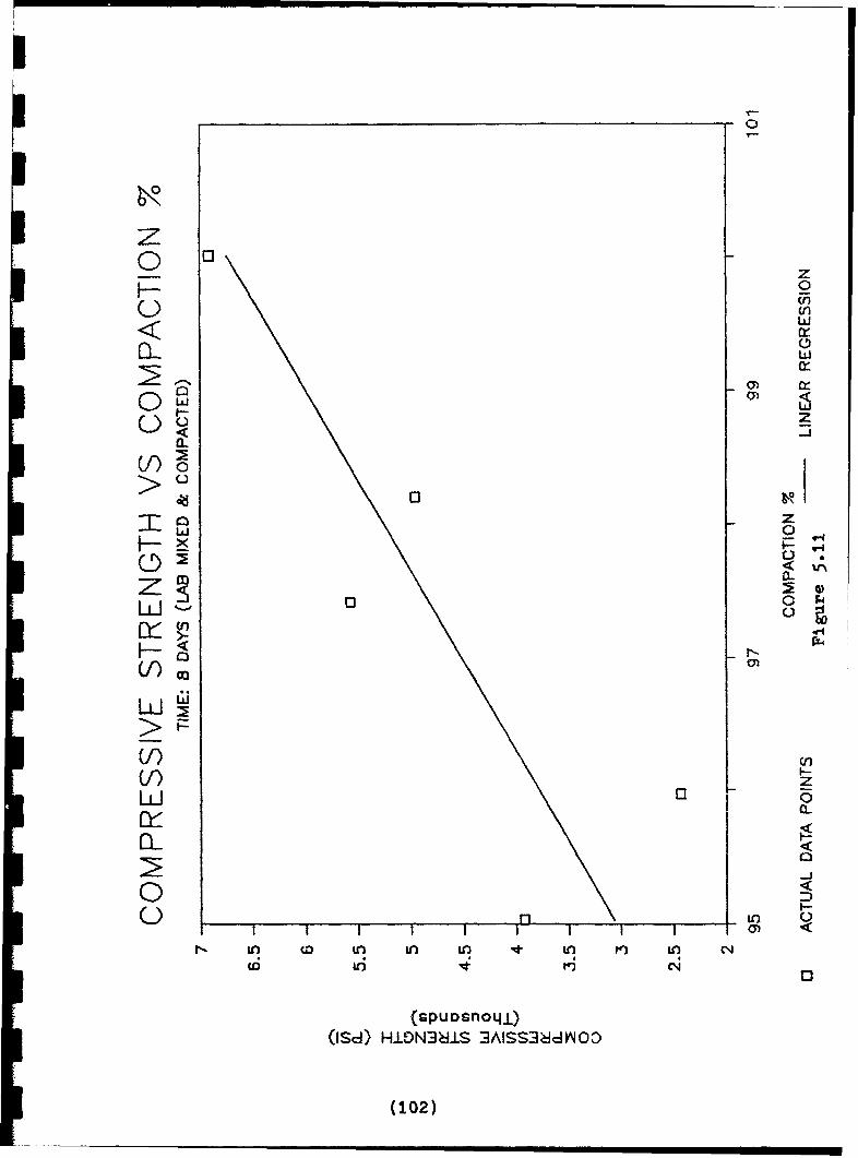
0z o0w<
a-r
C/)a
00
0 F
LL] 0
rZ4
(I) z
D0• CI-
0 D0
(9nr- U3 co LO Ln U13 0j U 4') U,) C14
CD 4 "i j
(Spuor~noiL.±)(Isd) HLDN3J:LS 3AISSdý1NOO
(102)

'II The field mixed and laboratory compacted samples tested
I at 14 hours (SC, SC, 70, 8C) yielded a very small amount of
scatter of compressive strengths. The results were processed
I through linear regression to obtain a simplified linear
relationship. The linear relationship shows that the
strength slightly decreased as compaction increased. The
3 closeness of the compaction percentages (S6.8% to 97.6%)
idicates that the compaction increases from sample to
3 sample were not significant enough to overcome other factors
such as poor mixing that could cause small drops in
U compressive strength. Figure 5.12 shows the points and the
* linear relationship.
The field mixed and laboratory compacted samples tested
3 at 211 hours (SC, IOC) yielded a very large amount of
difference of compressive strengths. The simplified linear
I elationship shows that the strength greatly increased as
3 compaction increased. The closeness of the compaction
perentages C9B.8% to S7.2%) indicates that the compaction
3 increases from sample to sample were not significant enough
to cause the large increases in compressive strength. The
3 combination of lower compaction and other factors
such as poor mixing could hay contributed to the low
strength of sample 9C. Figure 5.13 shows the points and the
linear relationship.
(IISi i i i i l I I | (103)I
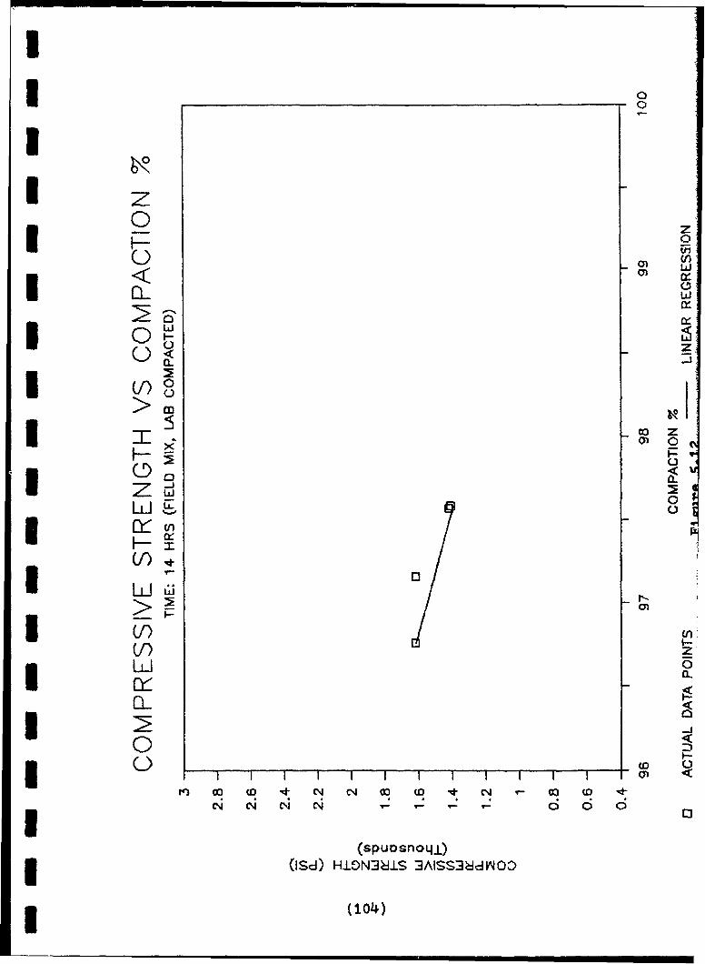
Iz
ILIL
(9)CL,I) 0~
>I
zo a<
zLi0Lli 0
10/33 D.ui
Ii a
0
Iý CO Ný Ný CO (03CO
(spuosno4La)3(ISdl) HION3ýJIS 3AISS3ýJddvOO
(104)

U)0.
0 0I)0
ItIV) *04
UI)
0
(spuoDsnotaL3 (ISd4) HION3ý11S 3AISS3J1dk4OO
3 (105)

3 The field mixed and compacted samples tested at 72
hours (12C, 13C) yielded a very large amount of difference
of compressive strengths. The simplified linear
relationship shows that the strength greatly increased as
compaction greatly increased. The large differencr, of the
3 compaction percentages (92.0% to 97.3%) indicates that the
compaction increases from sample to sample were significant
3 enough to cause large increases in compressive strength.
However, the excessively high strength may also be affected
by improper mixing causing concentrations of cement
3 powder. Figure 5.14 shows the points and the linear
relationship.
3 The field mixed and compacted samples tested at 168
hours (14C, 15C) yielded a very small amount of difference
of compressive strengths. The linear relationship shows
i that the strength slightly increased as compaction slightly
increased. There was a small difference of the compaction
3 percentages (95.S% to 96.8%). Figure 5.15 shows the points
and the linear relationship.
(UIi
II (106)I| i||

00
IC 0Ii00L
009LLJ <2
U/)
I >-(f)3 LUJ
0
(spuosnotqj)3 (Is-d) HION3ý11S ]AISS3ddINOO
(107)

U)0-
W 0j
> 0<
00
018

5.6.2 Compressive Strenath Uersus Time
The mean compressive stress for each time interval was
obtained by averaging the strengths of the cylinders tested
at the particular time interval. The variance (War.) shows a
the percentage variation of each cylinder From the mean.
The amount (Amt.) was the magnitude in lbs that each sample
differed from the mean. Table 5.16 lists the aforementioned
parameters for the compressive cylinders along with the
method each cylinder was mixed and compacted by.
(lO)

Table 5.16 Mean Compressive Stresses
MeanCuring Compress
Time Time Mix Comp. Stress Uar. Amt.Cyl. (hrs) Cdays) Method Method (psi) (C) Clbs)
iC 21f 1.0 LAB LAB 3155 -q.6% -iqS
2C 24 1.0 LAB LAB 3155 -. 6% L5
3C 192 8.0 LAB LAB q440 -1i.7% -520
i 4 192 8.0 LAB LAB L±PI0 11.7% 520
sC 14 0.8 FIELD LAB 15i8 -6.I-i -98
BC 14 0.6 FIELD LAB 1518 -7.11; -1087C 14 0.6 FIELD LAB 1518 6.8% 103
8C 1 L 0.6 FIELD LAB 151B 6.81 103
SC 24 1.0 FIELD LAB 20q0 -29.4% -600
l0C 24 1.0 FIELD LAB 2040 29.'L% 600
liC 72 3.0 FIELD LAB N/A N/A N/A
Core
12C 72 3.0 FIELD FIELD 2605 36.3% S4S
13C 72 3.0 FIELD FIELD 2605 -36.3% -945
14C 168 7.0 FIELD FIELD 2q0 2.0% 50
15C 168 7.0 FIELD FIELD 2440 -2.0% -50
The scatter of compaction percentages for the lab mixed
and compacted samples was well-distributed. Figure 5.16
shows the average compaction percentage as one line and each
sample's compaction percentage. The left four points CIC,
IT, 2C, IB) are from the one-day compression tests, the
remaining five right points (3C, 2T, 2B, 4C, 3B) are from
the eight-day compression tests
(110)

mm
o0 0~
0
ULCN
00o
0~)
a--
4dk
040
oN 0
w
z
(0 U)0M5)M r
%_ 6OI~V0(111)

The average compaction percentages are very close to
the overall compaction average as shown in Table 5.17.
Table 5.17 Compaction and Compressive StrengthAverages (Lab Mixed and Compacted)
Curing Average CompressiveTime Compaction Strength
Wdays) %(psi)
1 97.5 3820
8 97.3 4760
Overall 97T.
Figure 5.17 shows average compressive strengths versus
the time of curing relationship for the lab mixed and
compacted samples. The compressive strength increases over
time as expected.
The scatter of compaction percentages for the field
mixed and laboratory compacted samples was minimal. Figure
5.18 shows the average compaction percentage as one line and
each sample's compaction percentage. The left Four points
(8C, 7C, SC, 6C) are from the 1'-hour (0.6 daUs) compression
test, the next two points (9C, 1OC) are from one day
compression test and the rightmost point (1iC) is from the
three day compression test.
(:12)
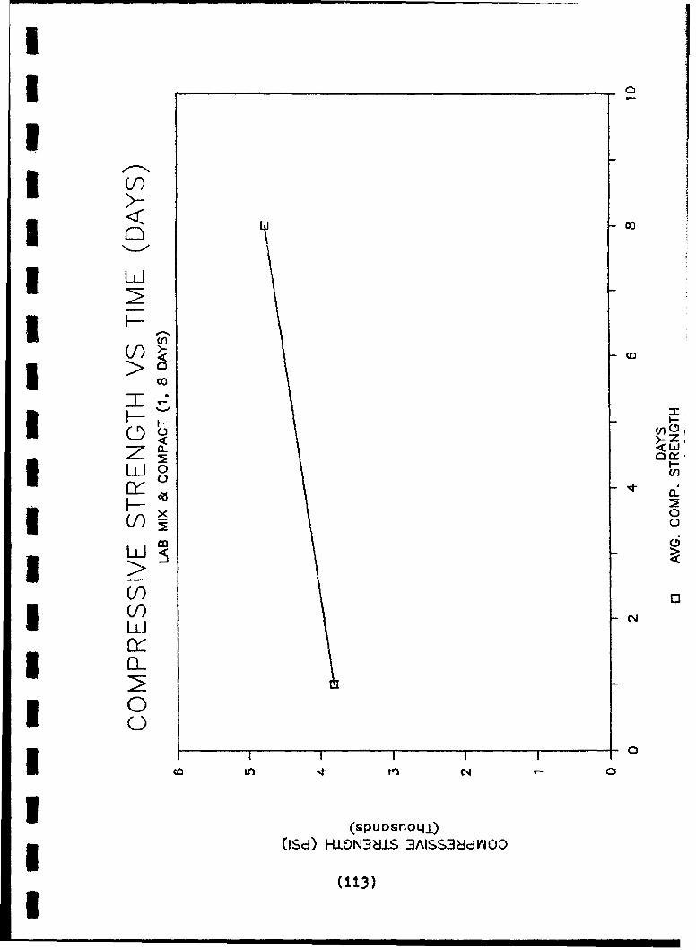
I C)
I w
3 0Z
C/) 0f)~ C14L-ci
0
(sPuD sn o qj)(ISdl) HION3ý11S 3AISS3,NdV4OO
(113)
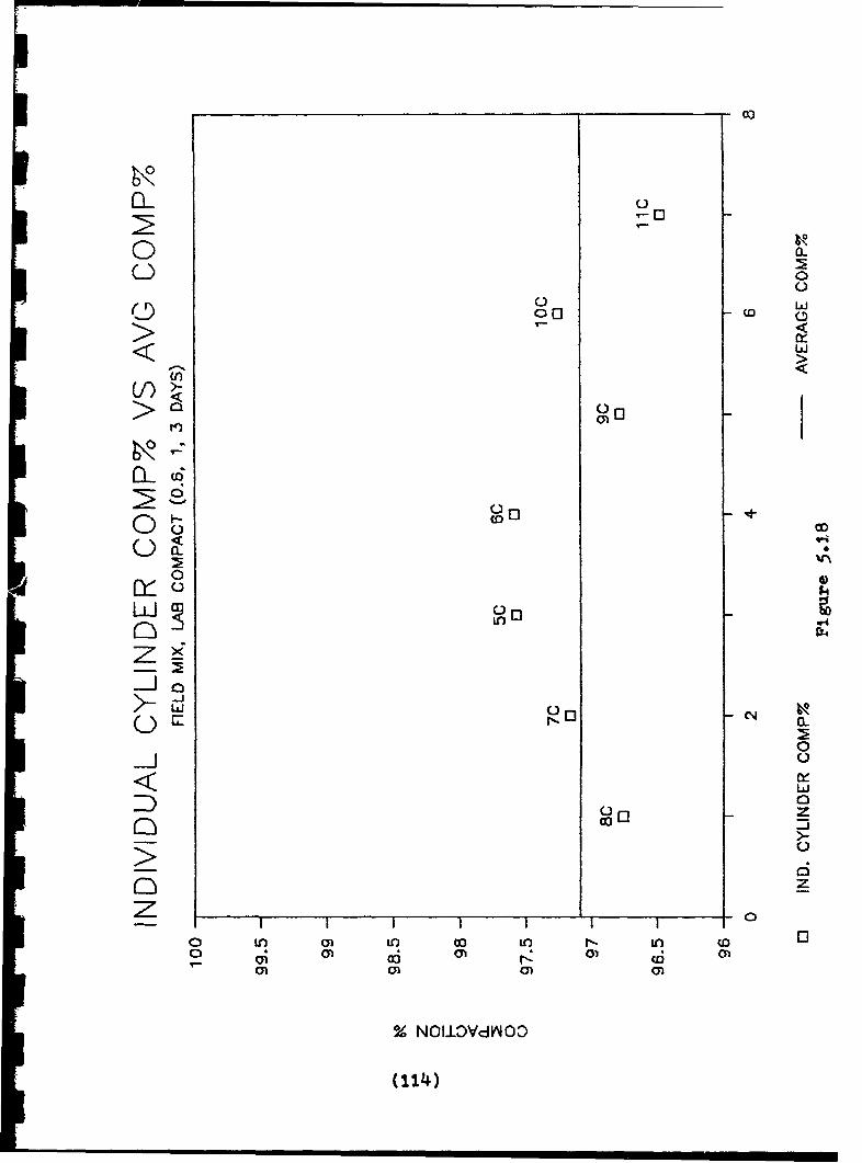
pn
00
0 wA00 CO
>2cr
00
4 4
Li 04
-JoJ
D; 06r.
m *l 01 i
Z NOI±OVdIVNOD
(114~)

II
The average compaction percentages are very close to
I the overall compaction average as shown in Table 5.18.
Table 5.18 Compaction and Compressive StrengthA-verages (Field Mixed and Lab Compacted)
I Curing Average CompressiveTime Compaction Strength
(days) % (psi)
0.6 97.3 1520
1 97.0 20O0
3 96.5 2730
Overall 97.4
I Figure 5.19 shows average compressive strengths versus
the time of curing relationship for the field mixed and
laboratory compacted samples. The compressive strength
increases over time as expected.
The scatter of compaction percentages for the field
mixed and compacted samples was large and maldistributed.
Figure 5.20 shows the average compaction percentage as one
line and each sample's compaction percentage. The left two
3 points (12C, 13C) are from the three-day compression tests.
The right two points (ICC, 15C) are from the seven-day
I compression tests.
III£ (115)

I (/)
<
I C/
1 04
ID NN
3L Wn
C/)~I Li)
>I 0 w
* 0C)
(spuosnot.4±)(ISd) HION3d±S 3AISS3addkOD
(116)

a-
o 0..
u C3 0
C)
< Lii
0f)
0C)0
NOC1 CN
L4.4
LLii
M..0
6Jz
ol (0I M" Nn 0) c l
(117)

In contrast, the average compaction percentages for
each test are close to the overall compaction average of all
cores as shown in Table 5.19.
Table 5.19 Compaction and Compressive StrengthAverages (Field Mixed and Compacted)
Curing Average CompressiveTime Compaction Strength
(days) % (psi)
3 S'i.7 2610
7 96.2 240
Overall 95.4
Figure 5.21 shows average compressive strengths versus
the time c: curing relationship for the field mixed and
compacted samples. The high strength of cylinder 12C at
35S0 psi, greatly increased the average compressive strength
of the three-day test. The use of high early strength
cement typically produces approximately 75% of the 28-day
strength at the three-day point (36). The strength
typically increases to 84% by the seven-day point (37). The
seven-day compressive strengths were clustered around their
strength of 24q0 psi creating an apparent 6.5% decrease in
strength from the three-day test average of 2610 psi.
Further discussion is presented in the conclusions
concerning this apparent erroneous result of decreasing
strength over time.
SC(118)
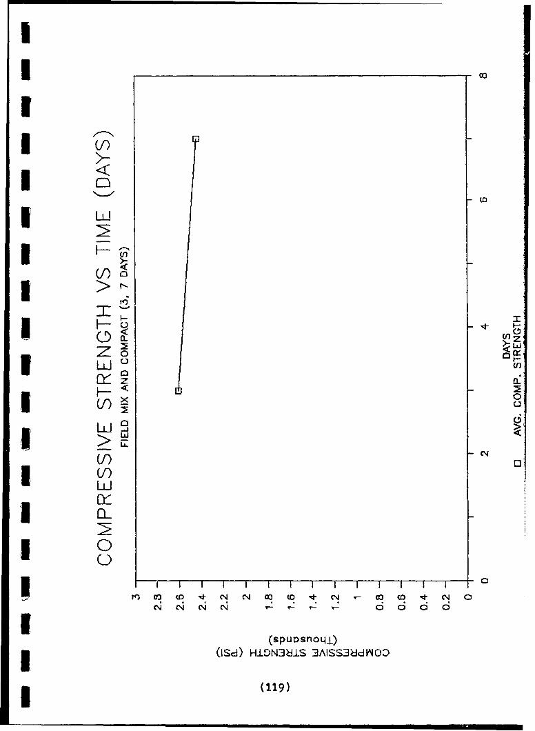
* 0')
z a:> w
LLJ~Zo3' Vn
0C)z
(IT C"'C
3 0ont4LwId iNaL AS3JIO
(0•9
Figure 5.22 shows the three compressive strength versus
time graphs superimposed upon one another. The ideal
laboratory mixed and compacted graph shows the expected
strength increase and overall higher strengths due to a lack
of error in material input, mixing, water addition, and
compaction. The field mixed and laboratory compacted graph
shows the expected increasing strength over time
relationship. The strengths are less than obtained in ideal
laboratory mixing conditions. The field mixed and compacted
graph shows the unlikely slight decrease in compressive
strength versus time relationship.
(120)
I ii I I " i i ii
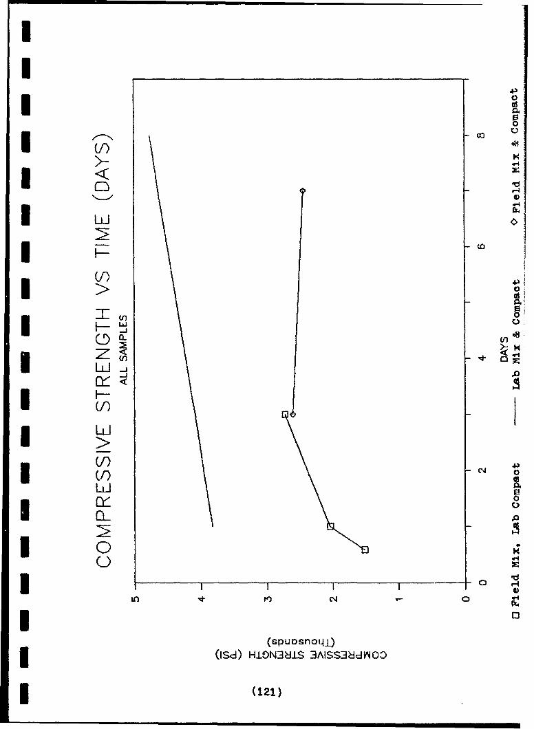
IVU4)
U) 4
v I 0
F4-
CfI)
V) 43
I ( 0
00u0
<44
*Id HINU 3-S8d4;
(11

CHAPTER 6
SENSITIVITY ANALYSIS
8.1 Introduction
An analysis was done on the following relationships:
1. Ihe effect of variation of Moist Rodded Unit
Weight (MRUW) on the ultimate layer thicknesses.
2. The effect of variation of the total water
application on the water to cement (W/C) ratio and moisture
content.
6.2 .MRUW Values to Lauer Thickness Relationship
The coarse aggregate moist rodded unit weight was
varied by +/- 10%. Taking into account the effect of the
angle of repose, which causes the trapezoidal shape of the
layers, the change in coarse aggregate height changes the
width of the top of the coarse aggregate layer that the fine
aggregate rests on Ccoarse is on bottom, followed by the
cement layer and then the sand layer). The change in
thickness of each layer along with the overall thickness of
the combined layers is tabulated in Table 6.1.
Table 6.1 Coarse Aggregate MRUW Sensitivity Analysis
Percent Change +10% +5% 0% -5% -10%
Coarse MRUW Cpcf) 100.Sq 85.87 81.40 86.83 82.26
Coarse Agg. Cin) L1.7 5.0 5.3 5.7 6.1
Cement Cin) 0.6 0.6 0.6 0.6 0.6
Fine Agg. Cin) 6.0 6.2 6.4 6.7 7.1
Total Thick Cin) 11.3 11.7 12.3 13.0 13.8
C122)
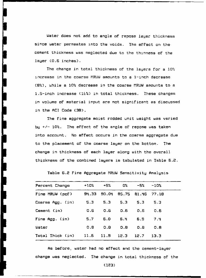
Water does not add to angle of repose layer thickness
since water permeates into the voids. The effect on the
cement thickness was neglected due to the thinness of the
layer (0.6 inches).
The change in total thickness of the layers for a 10%
increase in the coarse MRUW amounts to a 1-inch decrease
(8%), while a 10% decrease in the coarse MRUW amounts to a
1.5-inch increase C1L%) in total thickness. These changes
in volume of material input are not significant as discussed
in the ACI Code (38).
The fine aggregate moist rodded unit weight was varied
by +/- 10%. The effect of the angle of repose was taken
into account. No effect occurs in the coarse aggregate due
to the placement of the coarse layer on the bottom. The
change in thickness of each layer along with the overall
thickness of the combined layers is tabulated in Table 6.2.
Table 6.2 Fine Aggregate MRUW Sensitivity Analysis
Percent Change +10% +5% 0% -5% -10%
Fine MRUW (pcf) 9t.33 90.Oq 85.75 81.46 77.18
Coarse Agg. (in) 5.3 5.3 5.3 5.3 5.3
Cement (in) 0.6 0.6 0.6 0.6 0.6
Fine Agg. (in) S.7 6.0 6.'½ 6.9 7.
Water 0.8 0.8 0.8 0.8 0.8
Total Thick (in) 11.6 11.9 12.3 12.7 13.3
As before, water had no effect and the cement-layer
change was neglected. The change in total thickness of the
(123)

layers for a 10% increase in the coarse MRUW amounts to a
0.7-inch decrease CS%), while a 10% decrease in the coarse
MRUW amounts to 1-inch increase C8%) in total thickness.
These changes in volume of material input are not
significant as discussed in the ACI Code C39).
6.3 Total Water Application to W/C Ratio and
Moisture Content Relationships
The total amount of water added is controlled by the
flowrate of the water and the speed of the watertruck. The
flowrate of water and the watertruck speed were varied by
+/- 10% to gauge the effect on the water to cement (W/C)
ratio and overall moisture content. Table 6.3 tabulates the
effects of flowrate variation.
Table 6.3 Flowrate Sensitivity Analysis
Percent Change +10% +S% 0% -S% -10%
Flowrate Cgal/sec) 2.14 2.O04 1.SLi 1.84 1.75
Uolume of Water 236 225 215 204 183Placed Cgal)
Water/Cement Ratio 54.q% 51.7% 48.9% '6.1% "&3.4%
Mcisture Content S.5% 5.2% L.9% . .7% Li.'*%
Table 6.4 tabulates the effects of watertruck speed
variation.
C12L9)

Table 6.4 Watertruck Speed Sensitivity Analysis
Percent Change +10% +5% 0% -S% -10%
Uelocity (ft/sec) 1.79 1.71 1.63 1.55 1.46
Uolume of Water 19S5 204 215 226 239Placed (gal)
Water/Cement Ratio 43.9% 46.3% 4B.9% 51.8% 55.0%
Moisture Content 'i.5% 4.7% 4.9% 5.2% 5.5%
The range for the water to cement ratio is 36% to 60%.
The low end of 36% is the lowest W/C ratio that typically
permits full hydration of all cement powder (40). The high
end oF 60% is the maximum W/C ratio allowed according to ACI
Code (41). The variations on the W/C ratios clearly Fall
within the acceptable range.
The maximum moisture content recommended is
approximately 6% (42,43). The controlling Factor is the
required stiFfness For compactive eFForts by vibratory
roller.
(125)
ICHAPTER 7
CONCLUSIONS AND RECOMMENDATIONS
7.1 Conclusions
The CPM diagram details a construction sequence that
3 takes approximately 2.25 hours to complete. The pavement
may be used at +2.25 hours, however, rutting of
3 approximately l.S- to 2-inches will occur and should be
rolled out within 30 minutes after occurring. If at least
I one hour of curing time is allowed after vibratory roller
i compaction, no settlement will occur due to a W00 psi stress
which is the maximum wheel stress anticipated. Therefore,
5 the pavement would be fully usable after approximately 3.25
hours from the beginning of construction. It is concluded
I I that most of the strength of the concrete at the early time
of +3.2S5 hours is due to the strength of the aggregates
acting as a base course with minimal additional strength
3 from concrete set. Therefore, compaction of the subgrade
below the aggregates is required to provide additional
3 resistance against settling. Further study should be
completed to determine the long-term effect of such early
use on the durability of the concrete after set. In an
3 Iemergency situation over several days, the short-term use is
unlikely to be hindered.
I It is concluded that this method is superior to
existing methods of runway repair since it requires no
maintenance once placed (disadvanatge of crushed stone),
3 provides a smooth interface with existing pavement
(disadvantage of AM-2 matting), resists differential
3 (126)
II3 settlement (pro-cast concrete slabs), and can rapidly
produce large amounts of zero slump concrete (disadvantage
1 of Cretemobile).
3 The mix design was capable of producing strengths of
3000 psi and above within 24 hours when properly
3 proportioned, mixed, and compacted. This was evidenced by
compressive tests conducted at 2q hours after mix
U preparation.
3 One of the most influential factors in this method is
judged to be the degree of mixture of the concrete
3 materials. Establishing reliable accurate mixing
performance criteria would require extensive testing and
U analysis, therefore this performance criteria was not
i measured in the field test due to the limit of resources,
time, and effort of personnel performing the field test.
3 However, it is obvious that if the layers were not mixed at
all, no strength would develop in the slab. Conversely,
I perfectly mixed material possesses the potential of
attaining the anticipated mix design strength. The degree
of mixing actually performed lies somewhere in between
3 the two extremes with some irregularity in certain areas.
Irregular mixing could cause an excess of concrete powder in
3 one area possibly producing a very high strength sample and
a lack of cement powder in another area producing a very
* weak sample.
3 Results from lab mixed and lab compacted cest specimens
are conclusive showing an increase in unit weight causes an
3 (127)

II3 increase in compressive strength. The compressive strength
increased over time as expected from the 1 day to 8 day
compression tests. The unit weights were well-distributed
3 producing similar average unit weights from the one-day test
to the eight-day test.
Results from the field mixed and lab compacted samples
were conclusive for compressive strength versus time
relationships, but inconclusive for compaction to
compressive strength relationships. The unit weights were
clustered together Caround 0.8% spread) producing similar
average weights from the 1i-hour test to the 24- and 72-hour
tests. The clustering of unit weights also produced a
clustering of compressive strengths (+/- 100 psi) for the
1q-hour compression test. The slight decrease in
compressive strength as compaction increased is concluded to
be erroneous. It is concluded that the small decrease in
compressive strength was caused by irregular mixing. The
24-hour test showed an increase in compressive for a small
increase in compaction. Therefore, it is concluded that the
24-hour test was affected by other factors such as improper
mixing which caused concentrations of cement powder
producing higher and lower strength samples. The
compressive strengths increased over time as expected.
The results from the field mixed and lab compacted were
conclusive in showing a compressive strength increase versus
increasing compaction. However, the compressive strength
versus time results indicated an erroneous trend of slightly
C128)

decreasing strength over time. This result is concluded to
be due to the high strength of 3550 psi for the 12C
sample which raised the three-day test average strength to
2610 psi vice the expected value of approximately 2200 psi.
The high strength is concluded to be due to possible
improper mixing providing excess cement powder. The 12C
sample also had the highest degree of compaction for the
field mixed and compacted tests, thereby raising the
compressive strength. The seven-day average compressive
strength was 2440 psi creating an apparent 6.5% decrease in
strength from the three-day test average of 2610 psi. The
expected result was an increase of approximately 9% in
strength from the three- to seven-day tests. Therefore, the
total deviation from the normal was approximately 15%.
It is concluded that variations of the moist rodded
unit weights of +/- 10% will not significantly affect the
strength of the final mix.
A variation of +/- 10% in the flowrate or
watertruck speed will also not significantly affect the
final strength of the mix. The 10% increase in water
applied will also not significantly affect the stiffness of
the final mix, thereby allowing the use of vibratory
equipment.
7.2 Recommendations
For future testing of this procedure, it is recommended
that dry specific gravity tests and absorption tests be
performed on the fine and coarse aggregates in accordance
(129)

3 with ASTM standards (ASTM C127 & C126) to use for the volume
oE solids calculation. This will allow a closer check (than
the void ratio check) on the following:
1) Moist rodded unit weight (MRUW) calculation by
using the MRUW value to calculate the weight of solids CWs)
and using tt- dry specific gravity to calculate a volume of
solids (Vs).
I 2) Use the absorption parameter obtained from
in-house testing and calculate a saturated surface dry
specific gravity (SSDSG).
3) Check the values calculated for SSDSG against the
SSDSG parameters obtained From the aggregate company's
published laboratory results. Also check the absorption
parameters obtained by in-house testing against aggregate
company's published laboratory results. The calculated
3 values should check within 1% or other appropriate amount as
determined by sensitivity analysis.
The layer mixing method relies on the use of zero
slump, roller compacted concrete. The zero slump concrete
could be made quicker for small quantities by using a small
portable mixer CIBS mixer). The breakeven quantity C+/- cy)
at which the layer mixing method surpasses the small mixer
I in production needs to be found. This will allow a
selection of methods based on the known quantity of concete
needed.
A criteria for degrees of mixing could be developed.
Using the degrees of mixing, test specimens could be
(i30)
prepared (four samples for each degree of mixing). Strength
versus degrees of mixing relationships could be developed
from test results. The degrees of mixing should be
delineated as to mixing of aggregates with cement powder and
mixing of mixed aggregates and cement powder with water. To
be useful, descriptive definitions of appearance of the
mix for each degree of mixture must be developed so that
field personnel can :ompetently relate the appearance of the
mix in the field to a particular degree of mixture.
The field mix and compaction combination could be
tested in a manner to insure a broad range of unit weights
for each time interval tested. This will allow a more
controlled comparison of unit weight versus compressive
strength analysis. The test slab should be approximately
five ft wide and ten roller widths long. The vibratory
roller could then be used to compact each roller width
length of the slab at different numbers of passes thereby
creating different unit weights. The vibratory roller could
start from one end traveling across the width of the slab
for one pass down to the far end of the slab where ten
passes across the width of the slab would be made. Core
samples could then be cut from each section. A minimum of
five laers should be cut from each section to provide
sufficient samples to allow for sample deviations. The
samples could be tested for compressive strength. Beams
could also be cut and tested for flexural strength.
Since the slab will most likely be used within the
(131)
FircL few hours after construction, the rupture strength of
the concrete will be minimal, therefore cracking of slab
will occur. To further analyze the crack formation and
ensuing settlement requires a finite element analysis. The
finite element analysis should be done for different
aircraft wheel loads (C-5, C-141, F-14, etc..) and slab
configurations. The research goal would be to determine the
degree of differential settlement that could occur in
certain loading situations.
The use of a paver could also be used to lay down the
aggregates using the external equivalent hole concept. For
a large number of crater repairs, the paver may become very
beneficial in speeding up layer placement.
(132)
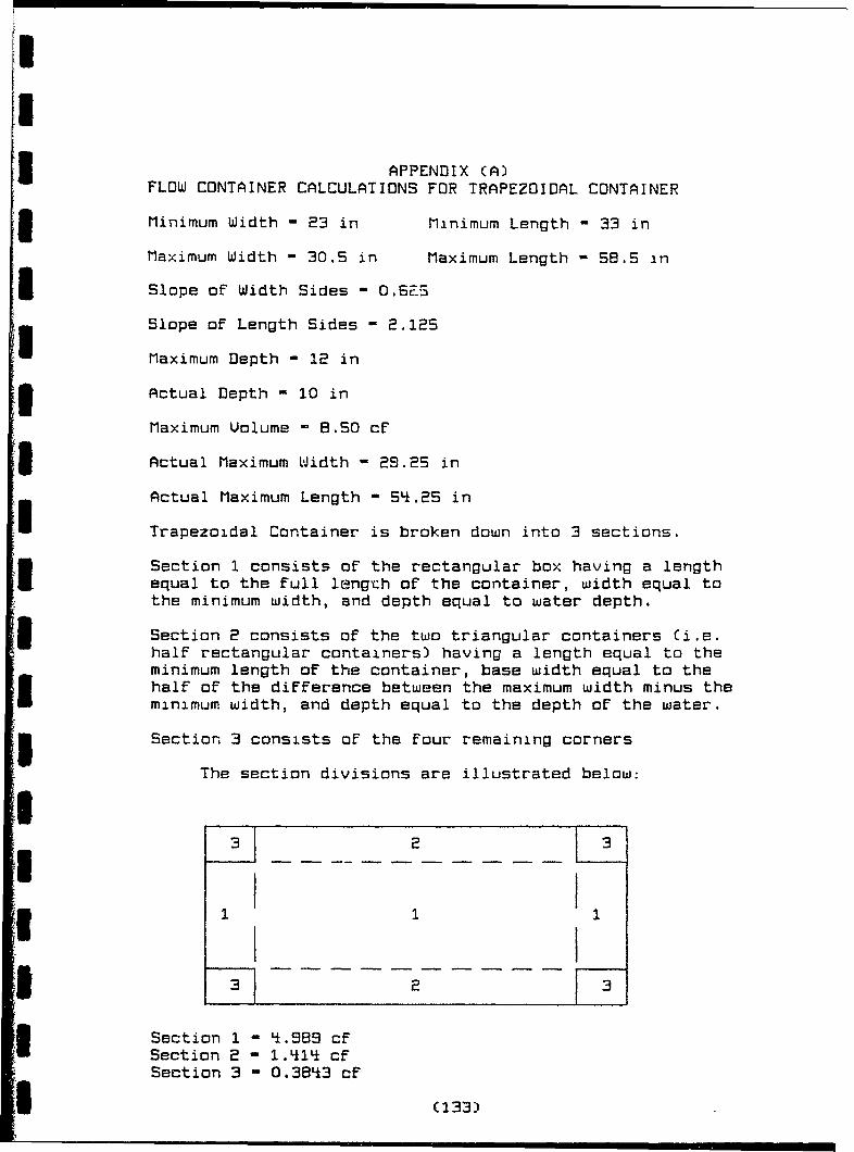
APPENDIX CA)FLOW CONTAINER CALCULATIONS FOR TRAPEZOIDAL CONTAINER
Minimum Width - 23 in Minimum Length - 33 in
Maximum Width - 30.5 in Maximum Length - 5B.5 in
Slope of Width Sides -O.S
Slope of Length Sides - 2.125
Maximum Depth - 12 in
Actual Depth 1 10 in
Maximum Uolume - B.SO cf
3l Actual Maximum Width = 29.25 in
Actual Maximum Length -54.25 in
Trapezoidal Container is broken down into 3 sections.
Section . consists of the rectangular box having a lengthequal to the full length of the container, width equal tothe minimum width, and depth equal to water depth.
Section 2 consists of the two triangular containers Ci.e.half rectangular containers) having a length equal to theminimum length of the container, base width equal to thehalf of the difference between the maximum width minus theminimum width, and depth equal to the depth of the water.
.5 Section 3 consists of the four remaining corners
The section divisions are illustrated below:
I
73 2 3
IIi3 '1 1
Section 1 - 4.989 cfSection 2 - 1.414 cfSection 3 - 0.3843 cf
(133)

Total - 6.787 cF
ActUolume 50.7B gal
U4 -,i)

ii
APPENDIX (B)CALCIUM CHLORIDE APPLICATION
Assumes all Calcium Chloride is placed.
Calcium Chloride Cont'ent - 32 lbs
3 Total Driving Time - Ill sec
Application Rate - 0.293 lbs/sec
3 Total Uolume of Dilution Water - 10 gal
Concentration Calcium Chloride - 3.242 lbs/gal
Calc'd Application Rate - 0.090 gals/sec
Calc'd Application Rate - 11.06 secs/gal
Calcium Chloride Placed by Weight - 1.00%
IUi1I3UIiI1 (135)

APPENDIX CC)MATERIAL REQUIREMENTS
Actual Crater Uolume 8 8.3 Cy
Uolumes in Place I Cy 8.3 Cy
Coarse Aggregate 0.751 Cy 6.256 Cy
Fine Aggregate * 0.599 Cy q.9BS Cu
* Includes FLUFF of aggregates
BASE COARSE OF COARSE AGGREGATE = 2 in
Extra Coarse Aggregate Required - 1.67 cy
Bags of TYPE III Cement Req'd - 34 bagsAdd extra bags to prevent running short.
MATERIAL SUMMARYRequired On Hand Reserve
Ccy) (cy) Ccy)Coarse Agg. 7.92 10.00 2.08
Fine Agg. L1.99 10.00 5.01
" Cement Cbags) 3Lf.If9 50.00 15.51
C136)
[1I I I
II1
APPENDIX (D?IUNIUERSAL ENGINEERING TEST RESULTS
I,
I17
I

I offices InS• Orlancdc
UNIVERSAL Ga1ies InENGINEERING SCIENCES F Myers
U Consuitan's In Geolechnical Engineerinc 1" 5. D a~,~ Z'Environmental Sciences • Construction Materials Testing B ' . -
Ii
February 22, 1990
Kaco Contracting Company1911 Silver Star RoadOrlando, Florida 32804
Attention: Mr. Richard Coble
Reference: Roller Compacted Concrete Test Strip1911 Silver Star RoadOrlando, FloridaProject Number: 15281-001-O1CMTReport Number: 2712 Reissued: 03-28-90
Dear Mr. Coble:
As requested, on February 12, 1990, Universal Engineering Sciences (UES)obtained six (6) additional cores test specimens from the roller compacted con-crete test strip at the above noted site to be cut, capped, and tested forweight, volume, and compressive strength. The cylinders were also tested forweight, volume, and compressive strength yielding a comparison between thecylinders and field cores concrete.
'5 The cores were obtained on February 12, 1990, utilizing a rotary drill diamondcore bit and test for compressive strength on the following dates:
3 day test on 2/12/90,7 day test on 2/16/90,28 day test on 3/9/90.
3 All pertinent core test data is provided in tabular form on the accompanyingsheet titled "Report on Compressive Strength on Hardened Concrete." The datapertinent to the field compacted cylindrical concrete specimen is as follows:
II
3532 Maggie Blvd. • Orlando, FL 32811 • (407) 423-0504(138)

Project No.: 15281-001-01CMTReport No.: 2712
______ __.... Cylinder No.
0 00
L %0 L" > CD CO m.. Volume (ft3)
w %D P_ . w Cn -P Unit Weight (pcf)
w 0 0D O %0 0a 0lio4 L" -i -A
o Co C L" C U -Before Cap 0eight (i0.)
U, C '.0 After Cap Veight (iue .)
Cl I. O-
o a. 0 a- 0 - - oa oa ls.
- 0 0 U ' - O•
PQ C P. OBefompress UnWeightr(ent)
0 D 4m Beforer Cap Weight (ing.)
(' -) 0ý Afte CD C Dam eight (in.)
Po ageo 2o of cCD 0% CD O 4:b
CD CD. a a- Co r ct-F c o
__b, __ _ __:bL/
o -c~o 0$_&-~ .~
o 0 0 U' U' Correctio eaco
I I- Coprssv Stent
Pag 2 of 4 Pages
~.J U(139)

,_ I g
o 0 r o Q C
0 C%J C'.J -40c,
0 V))
00r0 C0
4-C) CI C>J C1 -0 CD C C D I C
t0-4 M%
0
4-4)
LU @0 Io m I~ -4 I>
CSL _ _ CSJ 13 - C%J .l4 4n
rn * c
C~j C'I 0i C' '.
1_ .103 4-
Col
CV)L
II _ _r _ _ _ _ __UI ; ýS.- LA C004
0Co) 1.0 1 n oQ0 00.F 4-- 9* a%/) C) 000 4m
w V LO to% o %
0 a *ý co _ o ý r
LJ.I * 000 0(%j fS-. LC) V- "a. "aS. cII
4J 0n -m -o 0 000 0o4- V) -4 4- +A A - C - CL).) 4J
=D)I 3c a- I-r CV) Q10
-4.04'- 4 -- -4
a; eJ CV L
(;C C

Project No.: 15281-001-O1CMTReport No.: 2712
In review of the data on the test strip cores and the compacted concretecylinder, the compacted concrete cylinders indicate similar compactive efforton each sample even though the height was varied. The unit weights of thecores and cylinder were similar, yet the compressive strength varied greatly.
We trust the presented information satisfies your immediate needs. However, ifyou should have any questions, please feel free to call.
Respectfully submitted,
Mark NaughtonLaboratory SupervisorUniversal Engineering Sciences
Fre J l ,PECMT -Tgi eering ManagerUniversal Engineeiing Sciences
MN:FJS:rls
cc: Client (2)Paul Soares (1)MN, UES (1)
iw
Page 4 of 4 Pages(141)

APPENDIX (E)
CONCRETE TEST RESULTS
Table E.1 Compressive Strength Data Sheet
UnitDiam. Ht. uol. Wt. Wt. Comp.
Cul. (in) (in) (cf) (Ibs) Cpcf) M•)IC Lf 6.32S 0.0460 6.318 137.1 94 .6%2C Li 5.975 0.0i35 6.263 lqq.1 99.3%3C Li 6.325 0.0i60 6.347 138.0 95,0%LiC Li 6.475 0.0q71 6.715 142.6 98.2%
SC 6 7.894 0.1292 18.30 141.7 97.6%6C 6 8.i88 0.1389 19.68 1l1.7 97.6%7C 6 7.875 0.1289 18.16 141.1 97.2%BC 6 8.708 0.1425 20.02 140.5 96.8%
9C 6 9.108 0.1q90 20.9q 1L0.5 96.8%
lOC 6 8.865 0.1451 20.48 141.2 97.2%
IIC 6 9.320 0.1525 21.36 1i0.1 96.5%
Core12C 2.77 7.000 0.0244 3.qS0 141.3 97.3%13C 2.77 6.500 0.0227 3.030 133.6 92.0%
15C 2.77 5.500 0.0192 2.696 140.5 96.8%15C 2.77 8.250 0.0288 3.990 138.6 95.5%
Init. Corr.Comp. Red. Comp.
Load Area Stress Factor StressCylinder (ibs) (in^2) (psi) M•) (psi)
iC 39Li90 12.566 3140 0.9600 30102C 4L6SO 12.566 3550 0.9300 33003C 51230 12.566 L080 0.9600 39204C 65010 12.566 5170 0.9600 4960
SC 42500 28.27L 1500 0.9855 14206C 41500 28.27q 1L70 0.9560 1107C q8250 28.27L 1710 0.94i5 16208C q7750 28.27L 1690 0.9600 1620
9C 42000 28.274 1490 0.9670 1440lOC 77250 28.27L 2730 0.9660 2640
11C 79500 28.27q 2810 0.9700 2730Core
12C 21400 6.026 3550 1.0000 355013C 10000 6.026 1660 1.0000 16601iC 15000 6.026 2490 1.0000 249015C 1ViO0 6.026 2390 1.0000 2390
(142)

APPENDIX FCOMPRESSIVE STRENGTH GRAPH DATA
TABLE (FI) - Graph Summary oF Calculated and ActualStrengths
PRIMARY SORT ON CURING TIME,SECONDARY SORT ON COMPACTION
SPEC. COMP FLEX TENS COMPACT'N TIME AUGS.(%) (HRS) Y REU.
iC 3010 552 301 9q.6% 2q 2973 3820IT 35'6 567 355 96.1% 2q 3059 97.5%2C 3300 LISS 330 99.3% 24 43361t lB 5405 811 507 100.0% 2q 5555
3C 3920 588 392 95.0% 192 3066 47602T 2435 390 243 96.0% 192 3763 97.3%2B 5576 836 523 97.1f% 192 q828
C 45360 7L*'* 496 98.2% 192 540838 6914 1037 648 100.0% 192 6739
6C 1620 2'*3 162 96.8% 14 161q 15207C 1620 2'-3 162 97.2% 14 1S07SC 11f20 213 142 97.6% 14 13986C 1'10 212 141 97.6% 1q 1394
9C 1LfLfO 216 1 *'-k 96.8% 2'* 204 030C 2640 396 264 97.2% 24
IIC 2730 '*10 273 96.5% 72 273013C 1660 2'-9 166 92.0% 72 261012C 3550 533 355 97.3% 72
15C 2390 359 239 95.5% 168 244014C 2'*90 374 249 96.8% 168
AVERAGE CORE COMPACTION 96.4%3FOR 3 & 7 DAY BREAKS)
(143)

Table CF2) Laboratory Nixed and Compacted Graph Data
COMP%CYLINDER IND. AVG ACTUALDATALABEL COMP% X-AXIS COMP% COMPRESSIVE
B-RANGE A-RANGE STRENGTHS0 97. If
1C SLf . 6 1 97. If1T 96.1 2 97 . Lf2C 99.3 3 97. 41B 100.0 Lf 97. 43C 95.0 5 97.1f 39202T 96.0 6 97. If 2Lf 3S2B 97 . Lf 7 97. Lf 557611C 98.2 8 97 . Lf LfS603B 100.0 9 97. Lf 6911f
10 97 . Lf
Table CF3) Laboratory Mixed and Compacted Graph Data
AVGCOMPRESS TIMESTRENGTH CDAYS)
3820 1Lf 760 8
Table CFq) Field Mixed and Lab Compacted Graph Data
CYLINDER IND. AVGDATALABEL CONP% X-AXIS COMP%
0 97.18C 96.8 1 37.17C 97.2 2 97.15C 97.6 3 97.16C 97.6 Lf 97.1SC 96.8 5 97.110C 97.2 6 97.111C 96.5 7 97.1
a 97.1
Table (FS) Field Mixed and Lab Compacted Graph Data
AVGCOMPRESS TIMESTRENGTH CDAYS)
1520 0.62040 1.02730 3.0

Table CF6) Field Mixed and Compacted Graph Data
CYLINDER IND. AUG ACTUALDATALABEL COMP% X-AXIS COMPF COMPRESSIVE
B-RANGE STRENGTH
0 96.12C 97.3 1 96.4 355013C 92.0 2 96.1f 16601'*C 96.8 3 96.'* 24901SC 95.5 I 96.1 2390
S 96.I
Table CF7) Field Mixed and Compacted Graph Data
AUGCOMPRESS TIMESTRENGTH (DAYS)
2610 3244 0 7
Table (F8) Average Compressive Strengths
FLCOMPDA - Field Mixed, Lab CompactedLLCOMPDA - Lab Mixed, Lab CompactedFFCOMPDA - Field Mixed, Field Compacted
DAYS FLCOMPDA LLCOMPDA FFCOMPDA0.6 15201.0 2040 38203.0 2730 If090 26107.0 Li630 2Li'i08.0 4760
(145)
REFERENCES1. Air Force Engineering and Services Center, Tyndall AFB,
Rarpid Runwau Repair Concept of Operations Florida,September 1988), p. 1-i.
2. Commander, Naval Construction Battalions, U.S. PacificFleet and U.S. Atlantic Fleet, COMCBPAC/COMCBLANTOPLAN 9000, (Norfolk, Virginia, July 1989), p. 1.
3. Commander, op. cit., p. C-UI-2.
4. Ibid.
S. Headquarters, Department of Army, Air Base DamageRepair (Pavement Reoair), (Washington, DC,December 1988), p. A-I1.
6. Commander, Do. cit., p. C-UI-A-1.
7. Soares, P. A., Coble, R. J. "Naster Activity Sequence"Conversation of Construction Procedures, Orlando,FL, 9 February 1990.
B. Coble, R. J., "Photographs of Field Test", Orlando, FL,9 February 1990.
9. Williams, R. I. T., Cement Treated Pavements:Materials, Desion. and Construction (New York, NY,Elsevier Applied Science Publishers LTD, 1986), p.SSS.
10. Allan, Charles, "Florida Mining Company AggregateSpecifications," Telephone Conversation at 4:00 PMon 9 January 1990.
11. Richardson, Daniel, "Miami Oulite Laboratory TestResults", Laboratory Report, University Florida,Gainesville, 25 January 1990.
12. Richardson, Daniel, "Natural Moisture Content TestResults", University Florida, Gainesville, 25January 1990.
13. Kosmatka, Stephen, H., Panarese, William, C., Designand Control of Concrete Mixtures (Skokie,Illinois, Portland Cement Association, 1988), p.36.
I4. Holtz, Robert, D., Kovacs, William, D., An Introductionto Geotechnical Enoineering (Englewood Cliffs, NewJersey, Prentice Hall Inc., 1981), p. 12.
1S. Kosmatka, oP. cit., p. 36.
16. Richardson, Daniel, "Natural Moisture Content TestResults", op. cit.
C i46)

I
17. Kosmatka, op. cit., p. 36.
18. Allan, Charles, "Florida Mining Company HggregateSpecifications," Telephone Conversation at 9:16 AMon 10 January 1990.
19. ACI Committee 207, "Roller Compacted Concrete"
20. Ibid.
21. ACI, oP. cit.. Fig 2.4.1, p. 7.
22. ACI, op. cit.. Table 2.3.2, p. 6.
23. Kosmatka, on. cit.. Table 4-3, p. 32.
21. ACl, op. cit.. p. 7.
25. ACI, n. cit... Table 2.2.1 p. 8.
26. Soares, P. A., Coble, R. J. "Equivalent Hole Concept,"Conversation of Construction Procedures, Orlando,FL, 9 February 1990.
27. "Caterpillar Performarnce Handbook," Edition No. 18,
Caterpillar Inc., Peoria, Illinois, 1987, p. 1i3.
28. Holtz, on. cit.. p. 177.
29. I
30. ASTM Committee C-9, "Method of Obtaining and TestingDrilled Cores and Sawed Beams of Concrete(CC2-84a)" American Society for Testing andMaterials, Philadelphia, 1985, p. 34.
31. Derucher, K. N. and Korfiatis G. P., Materials forCivil and Hiohwau Engineers, (Englewood Cliffs,New Jersey, Prentice Hall Inc., 1988), p. 105.
32. Ibid.
33. "Tests on Hardened Concrete," Notes for ECI3'iO3;LabManual (Unpublished Report), University ofFlorida, Gainesville Florida, 1989, p. 2q.
34. Ibid.
35. Ibid.
36. Kosmatka, op. cit., p. 1689.
37. Ibid,
38. ACI, pp. cit.. p. 5.
C(147)
IIS39. Ibid.
40. Neville, A.M., Brooks, J.J., Concrete Technoloau (New5 York, NY, John Wiley & Sons, Inc., 1987), p. 108.
1i. ACI, op. cit.. p. S.
3 '2. Packard, Robert, Telephone Conversation at 1:00 PM on20 December 1989.
5 ½3. ACI, op. cit._ Fig 2.4.1, p. 7.
I@I
IIII
i
I
C1i*8)