g. ferrari trecate - unipvsisdin.unipv.it/labsisdin/teaching/courses/ails/files/2... · g. ferrari...
TRANSCRIPT
Linear programming: introduction and examples
G. Ferrari Trecate
Dipartimento di Ingegneria Industriale e dell’InformazioneUniversita degli Studi di Pavia
Industrial Automation
Ferrari Trecate (DIS) Linear programming: introduction and examples Industrial Automation 1 / 42

Linear Programming (LP)
Widely used optimization technique in management science
optimal allocation of limited resources for maximizing revenues orminimizing costs
Basic problem
mingi (x)≤0
i=1,2,...,m
f (x), x ∈ Rn (1)
A Linear Programming (LP) problem is (1) with
f (x) = cTx (linear cost)
gi (x) = aTi x − bi (affine constraints)
An LP problem is a convex optimization problem
Ferrari Trecate (DIS) Linear programming: introduction and examples Industrial Automation 2 / 42

Linear Programming (LP)
Canonical form
An LP problem is in canonical form if it is written as
minaTi x≤bi , i=1,2,...,mxj≥0, j=1,2,...,n
cTx
ormax
aTi x≤bi , i=1,2,...,mxj≥0, j=1,2,...,n
cTx
“≤” constraints and positivity constraints on all variables
Ferrari Trecate (DIS) Linear programming: introduction and examples Industrial Automation 3 / 42

PL - matrix notation
Vector inequalities
x ≤ 0 means
x1 ≤ 0
x2 ≤ 0
. . .
xn ≤ 0
ConstraintsaT1 x ≤ b1
aT2 x ≤ b2
. . .
aTmx ≤ bm
⇔ Ax ≤ b, A =
aT1aT2...aTm
, b =
b1
b2...bm
Ferrari Trecate (DIS) Linear programming: introduction and examples Industrial Automation 4 / 42

PL - matrix notation
LP problem in generic form
minAx≤b
cTx
LP problem in canonical form (LP-C)
minAx≤bx≥0
cTx
Ferrari Trecate (DIS) Linear programming: introduction and examples Industrial Automation 5 / 42

LP and management science
Typical decision problems in industry
Product mix
Diet problems
Blending problems
Transport problems
Product mix with resource allocation
Multiperiod production planning
Portfolio optimization
...
Ferrari Trecate (DIS) Linear programming: introduction and examples Industrial Automation 6 / 42

Product mix
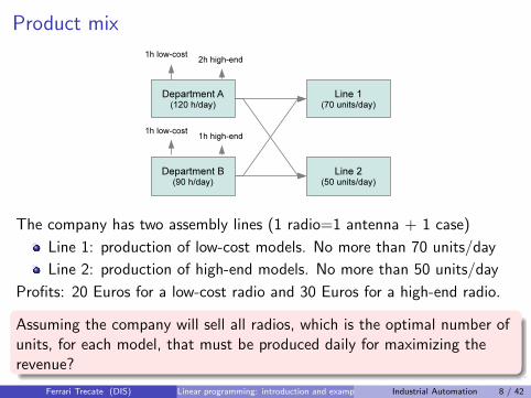
A company manifactures two radio models (low-cost and high-end) andproduces two components
Department A: antennas (max. 120h hours of production per day)
I 1h of work for a low-cost antennaI 2h of work for a high-end antenna
Department B: case (max. 90h hours of production per day)
I 1h of work for a low-cost caseI 1h of work for a high-end case
Ferrari Trecate (DIS) Linear programming: introduction and examples Industrial Automation 7 / 42
Product mix
The company has two assembly lines (1 radio=1 antenna + 1 case)
Line 1: production of low-cost models. No more than 70 units/day
Line 2: production of high-end models. No more than 50 units/day
Profits: 20 Euros for a low-cost radio and 30 Euros for a high-end radio.
Assuming the company will sell all radios, which is the optimal number ofunits, for each model, that must be produced daily for maximizing therevenue?
Ferrari Trecate (DIS) Linear programming: introduction and examples Industrial Automation 8 / 42

Product mix
Choice of variables
Usually this is the most difficult step in representing decision problems asoptimization problems !Guideline: cost and constraints must be a function of optimizationvariables only.
Ferrari Trecate (DIS) Linear programming: introduction and examples Industrial Automation 9 / 42

Product mix
Choice of variables - product mix
x1: number of produced low-cost radios per day
x2: number of produced high-end radios per day
Cost and type of problem
Cost: 20x1 + 30x2, to be maximized
Ferrari Trecate (DIS) Linear programming: introduction and examples Industrial Automation 10 / 42

Product mix
Choice of variables - product mix
x1: number of produced low-cost radios per day
x2: number of produced high-end radios per day
Cost and type of problem
Cost: 20x1 + 30x2, to be maximized
Ferrari Trecate (DIS) Linear programming: introduction and examples Industrial Automation 10 / 42

Product mix
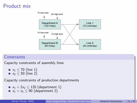
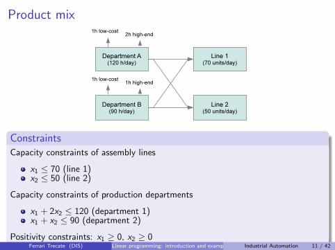
ConstraintsCapacity constraints of assembly lines
x1 ≤ 70 (line 1)x2 ≤ 50 (line 2)
Capacity constraints of production departments
x1 + 2x2 ≤ 120 (department 1)x1 + x2 ≤ 90 (department 2)
Positivity constraints: x1 ≥ 0, x2 ≥ 0
Ferrari Trecate (DIS) Linear programming: introduction and examples Industrial Automation 11 / 42
Product mix
ConstraintsCapacity constraints of assembly lines
x1 ≤ 70 (line 1)x2 ≤ 50 (line 2)
Capacity constraints of production departments
x1 + 2x2 ≤ 120 (department 1)x1 + x2 ≤ 90 (department 2)
Positivity constraints: x1 ≥ 0, x2 ≥ 0Ferrari Trecate (DIS) Linear programming: introduction and examples Industrial Automation 11 / 42

Product mix
LP problem
maxx1,x2 20x1 + 30x2
x1 ≤ 70x2 ≤ 50
x1 + 2x2 ≤ 120x1 + x2 ≤ 90
x1 ≥ 0x2 ≥ 0
Ferrari Trecate (DIS) Linear programming: introduction and examples Industrial Automation 12 / 42

Product mix
LP problem
maxx1,x2 20x1 + 30x2
x1 ≤ 70x2 ≤ 50
x1 + 2x2 ≤ 120x1 + x2 ≤ 90
x1 ≥ 0x2 ≥ 0
LP problem - matrix notation
minAx≤bx≥0
cTxx =
[x1
x2
], c =
[2030
]
A =
1 21 11 00 1
, b =
120907050
Ferrari Trecate (DIS) Linear programming: introduction and examples Industrial Automation 13 / 42

Product mix revised
A company manifactures twomodels of cases for telephones(model 1 and model 2). Theproduction cycle comprises threephases with bounded resourcesthat must be allocated to the twoproducts
Each phase is modeled through the maximal availability of men-hours perday and men-hours required to process a single unit
Profits: 30 Euros for a model 1 unit and 20 Euros for a model 2 unit
Assuming all cases will be sold, which is the optimal number of units, for eachmodel, that must be produced daily for maximizing the revenue?
Ferrari Trecate (DIS) Linear programming: introduction and examples Industrial Automation 14 / 42

Product mix revised
Choice of variables
x1: n. of model 1 unitsx2: n. of model 2 units
Cost and type of problem
Cost: 30x1 + 20x2, to bemaximized
ConstraintsCapacity constraints in each phase
8x1 + 4x2 ≤ 640 (assembly)4x1 + 6x2 ≤ 540 (finishing)x1 + x2 ≤ 100 (finishing)
Positivity constraints: x1 ≥ 0, x2 ≥ 0
Ferrari Trecate (DIS) Linear programming: introduction and examples Industrial Automation 15 / 42

Product mix revised
LP problem
maxx1,x2 30x1 + 20x2
8x1 + 4x2 ≤ 6404x1 + 6x2 ≤ 540x1 + x2 ≤ 100
x1 ≥ 0x2 ≥ 0
LP problem - matrix notation
maxAx≤bx≥0
cTxx =
[x1
x2
], c =
[3020
]A =
8 44 61 1
, b =
640540100
Ferrari Trecate (DIS) Linear programming: introduction and examples Industrial Automation 16 / 42

Diet problem
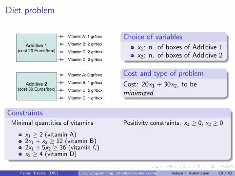
A company producing chickenfood can use two types ofadditives with different vitamincontents. The product is obtainedby mixing additives in a suitablequantity
Vitamin contents and additive costs are given in the picture
1 box of chicken food must contain at least 2 gr. of vitamin A, at least 12gr. of vitamin B, at least 36 gr. of vitamin C and at least 4 gr. of vitamin D
Which is the quantity of additives that allows the company to produce one box ofchicken food while minimizing the costs ?
Ferrari Trecate (DIS) Linear programming: introduction and examples Industrial Automation 17 / 42
Diet problem
Choice of variables
x1: n. of boxes of Additive 1x2: n. of boxes of Additive 2
Cost and type of problem
Cost: 20x1 + 30x2, to beminimized
ConstraintsMinimal quantities of vitamins
x1 ≥ 2 (vitamin A)2x1 + x2 ≥ 12 (vitamin B)2x1 + 5x2 ≥ 36 (vitamin C)x2 ≥ 4 (vitamin D)
Positivity constraints: x1 ≥ 0, x2 ≥ 0
Ferrari Trecate (DIS) Linear programming: introduction and examples Industrial Automation 18 / 42
Diet problem
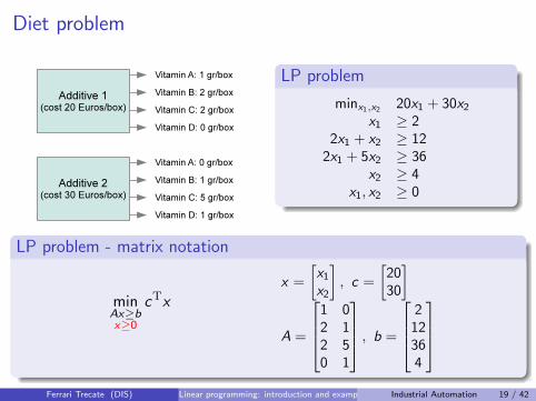
LP problem
minx1,x2 20x1 + 30x2
x1 ≥ 22x1 + x2 ≥ 12
2x1 + 5x2 ≥ 36x2 ≥ 4
x1, x2 ≥ 0
LP problem - matrix notation
minAx≥bx≥0
cTxx =
[x1
x2
], c =
[2030
]
A =
1 02 12 50 1
, b =
2
12364
Ferrari Trecate (DIS) Linear programming: introduction and examples Industrial Automation 19 / 42
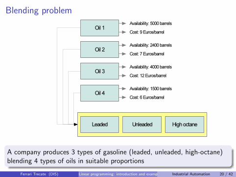
Blending problem
A company produces 3 types of gasoline (leaded, unleaded, high-octane)blending 4 types of oils in suitable proportions
Ferrari Trecate (DIS) Linear programming: introduction and examples Industrial Automation 20 / 42
Blending problem
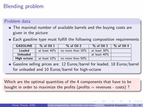
Problem data
The maximal number of available barrels and the buying costs aregiven in the picture
Each gasoline type must fulfill the following composition requirements
GASOLINE % of Oil 1 % of Oil 2 % of Oil 3 % of Oil 4
Leaded at least 40% no more than 20% at least 30%Unleaded at least 40%
High octane at least 10% no more than 50%
Gasoline selling prices are: 12 Euros/barrel for leaded, 18 Euros/barrelfor unleaded and 10 Euros/barrel for high-octane
Which are the optimal quantities of the 4 components that have to bebought in order to maximize the profits (profits = revenues - costs) ?
Ferrari Trecate (DIS) Linear programming: introduction and examples Industrial Automation 21 / 42

Blending problem
Choice of variables
xij : n. of barrels of oil i used for gasoline of type j , i = 1, 2, 3, 4,j ∈ {L,U,H}, L= Leaded, U= Unleaded, H= High-octane
Cost and type of problem
Cost to be maximized
124∑
i=1
xiL + 184∑
i=1
xiU + 104∑
i=1
xiH︸ ︷︷ ︸revenues
−
− 9∑
j∈{U,L,H}
x1j − 7∑
j∈{U,L,H}
x2j − 12∑
j∈{U,L,H}
x3j − 6∑
j∈{U,L,H}
x4j︸ ︷︷ ︸costs
Ferrari Trecate (DIS) Linear programming: introduction and examples Industrial Automation 22 / 42

Blending problem
ConstraintsMaximal availability of barrels
x1L + x1U + x1H ≤ 5000 (Oil 1)x2L + x2U + x2H ≤ 2400 (Oil 2)x3L + x3U + x3H ≤ 4000 (Oil 3)x4L + x4U + x4H ≤ 1500 (Oil 4)
Composition requirementsx1L
x1L+x2L+x3L+x4L≥ 0.4 in affine form 0.6x1L − 0.4x2L − 0.4x3L − 0.4x4L ≥ 0
x2L
x1L+x2L+x3L+x4L≤ 0.2 in affine form −0.2x1L + 0.8x2L − 0.2x3L − 0.2x4L ≤ 0
x3L
x1L+x2L+x3L+x4L≥ 0.3 in affine form −0.3x1L − 0.3x2L + 0.7x3L − 0.3x4L ≥ 0
x3U
x1U+x2U+x3U+x4U≥ 0.4 in affine form −0.4x1U − 0.4x2U + 0.6x3U − 0.4x4U ≥ 0
x1H
x1H+x2H+x3H+x4H≥ 0.1 in affine form 0.9x1H − 0.1x2H − 0.1x3H − 0.1x4H ≥ 0
x2H
x1H+x2H+x3H+x4H≤ 0.5 in affine form −0.5x1H + 0.5x2H − 0.5x3H − 0.5x4H ≤ 0
Positivity constraints: xij ≥ 0, i = 1, 2, 3, 4, j ∈ {U, L,H}
Ferrari Trecate (DIS) Linear programming: introduction and examples Industrial Automation 23 / 42

Blending problem
LP problem - matrix notation
maxAx≤bx≥0
cTx
with
x =[
x1L x2L x3L x4L x1U x2U x3U x4U x1H x2H x3H x4H
]Tc =
[3 5 0 6 9 11 6 12 1 3 −2 4
]T
A =
1 0 0 0 1 0 0 0 1 0 0 00 1 0 0 0 1 0 0 0 1 0 00 0 1 0 0 0 1 0 0 0 1 00 0 0 1 0 0 0 1 0 0 0 1
−0.6 0.4 0.4 0.4 0 0 0 0 0 0 0 0−0.2 0.8 −0.2 −0.2 0 0 0 0 0 0 0 00.3 0.3 −0.7 0.3 0 0 0 0 0 0 0 00 0 0 0 0.4 0.4 −0.6 0.4 0 0 0 00 0 0 0 0 0 0 0 −0.9 0.1 0.1 0.10 0 0 0 0 0 0 0 −0.5 0.5 −0.5 −0.5
b =
[5000 2400 4000 1500 0 0 0 0 0 0
]TFerrari Trecate (DIS) Linear programming: introduction and examples Industrial Automation 24 / 42

Transport problemProblema del trasporto
ESEMPIO 5 :
! "
! #
! $
! %
& "
& %
& $
E il problema dei depositi/distributori di benzina gia introdotto. Lo riformuliamo inmodo piu strutturato. Dati
• si, i = 1, . . . , n, depositi di benzina (oppure: n unita produttive che realizzano lostesso prodotto)
• dj, j = 1, . . . , m, distributori di benzina (oppure: m depositi periferici che devonoessere approvvigionati dal sottosistema logistico aziendale)
A company owns n fuel storagepoints (i.e. n supply points) andit must supply m gas stations (i.e.m demand points). Every gasstation can be reached from allstorage points.
Data and requirements
Every storage point has a maximal availability of ai ≥ 0 i = 1, . . . , n liters offuel
Every gas station specifies a demand of dj ≥ 0, j = 1, . . . ,m liters of fuel
tij ≥ 0 is the cost for shipping 1 liter of fuel from storage point i to gasstation j
Ferrari Trecate (DIS) Linear programming: introduction and examples Industrial Automation 25 / 42

Transport problem
Problema del trasporto
ESEMPIO 5 :
! "
! #
! $
! %
& "
& %
& $
E il problema dei depositi/distributori di benzina gia introdotto. Lo riformuliamo inmodo piu strutturato. Dati
• si, i = 1, . . . , n, depositi di benzina (oppure: n unita produttive che realizzano lostesso prodotto)
• dj, j = 1, . . . , m, distributori di benzina (oppure: m depositi periferici che devonoessere approvvigionati dal sottosistema logistico aziendale)
Which are the optimal quantitiesof fuel to be shipped from eachstorage point to each gas stationin order to minimize transportcosts while fulfilling exactly thedemands ?
Ferrari Trecate (DIS) Linear programming: introduction and examples Industrial Automation 26 / 42

Transport problem
Choice of variablesxij , i = 1, . . . , n, j = 1, . . . ,m, n. of liters of fuel shipped from storage point i togas station j
Cost and type of problem
Cost to be minimizedn∑
i=1
n∑j=1
tijxij
ConstraintsMaximal availability of fuel at storage points∑m
j=1 xij ≤ ai , i = 1, . . . , n
Demand constraints∑ni=1 xij = bj , j = 1, . . . ,m
Positivity constraints: xij ≥ 0, i = 1, . . . , n, j = 1, . . . ,m
Ferrari Trecate (DIS) Linear programming: introduction and examples Industrial Automation 27 / 42

Transport problem
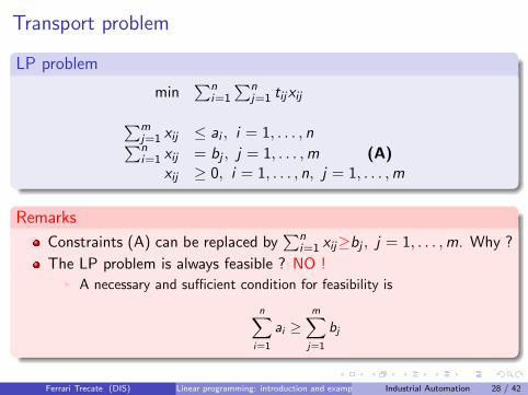
LP problem
min∑n
i=1
∑nj=1 tijxij∑m
j=1 xij ≤ ai , i = 1, . . . , n∑ni=1 xij = bj , j = 1, . . . ,m (A)
xij ≥ 0, i = 1, . . . , n, j = 1, . . . ,m
Remarks
Constraints (A) can be replaced by∑n
i=1 xij≥bj , j = 1, . . . ,m. Why ?
The LP problem is always feasible ? NO !I A necessary and sufficient condition for feasibility is
n∑i=1
ai ≥m∑j=1
bj
Ferrari Trecate (DIS) Linear programming: introduction and examples Industrial Automation 28 / 42

Transport problem
LP problem
min∑n
i=1
∑nj=1 tijxij∑m
j=1 xij ≤ ai , i = 1, . . . , n∑ni=1 xij = bj , j = 1, . . . ,m (A)
xij ≥ 0, i = 1, . . . , n, j = 1, . . . ,m
Remarks
Constraints (A) can be replaced by∑n
i=1 xij≥bj , j = 1, . . . ,m. Why ?
The LP problem is always feasible ?
NO !I A necessary and sufficient condition for feasibility is
n∑i=1
ai ≥m∑j=1
bj
Ferrari Trecate (DIS) Linear programming: introduction and examples Industrial Automation 28 / 42
Transport problem
LP problem
min∑n
i=1
∑nj=1 tijxij∑m
j=1 xij ≤ ai , i = 1, . . . , n∑ni=1 xij = bj , j = 1, . . . ,m (A)
xij ≥ 0, i = 1, . . . , n, j = 1, . . . ,m
Remarks
Constraints (A) can be replaced by∑n
i=1 xij≥bj , j = 1, . . . ,m. Why ?
The LP problem is always feasible ? NO !I A necessary and sufficient condition for feasibility is
n∑i=1
ai ≥m∑j=1
bj
Ferrari Trecate (DIS) Linear programming: introduction and examples Industrial Automation 28 / 42

Product mix with resource allocation
In standard product mix problems, capacity constraints are fixed. We nowassume to have resources that can be allocated to different productionphases
A food company produces 4products Pi , i = 1, 2, 3, 4. Eachproduct must go through 3production lines Lj , j = 1, 2, 3.Each line is modeled through theunits of work (u.o.w.) required toprocess a single unit of product
Ferrari Trecate (DIS) Linear programming: introduction and examples Industrial Automation 29 / 42

Product mix with resource allocation
Requirements
At least 1000 units of P2 and no more than 500 units of P1 must beproduced
U.o.w are men-hours that fall in 7 categories Ti , i = 1, . . . , 7 according tothe versatility of workers
Category Destination line Max. availability
T1 Line 1 12000T2 Line 2 7000T3 Line 3 9000T4 Lines 1 and 2 4000T5 Lines 1 and 3 3000T6 Lines 2 and 3 3000T7 Lines 1,2 and 2 2000
Profits per unit are 10 Euros for P1, 12 Euros for P2, 13 Euros for P3 and 14Euros for P4
Assuming all products will be sold, which is a joint production and resourceallocation plan that maximizes the profits ?
Ferrari Trecate (DIS) Linear programming: introduction and examples Industrial Automation 30 / 42
Product mix with resource allocation
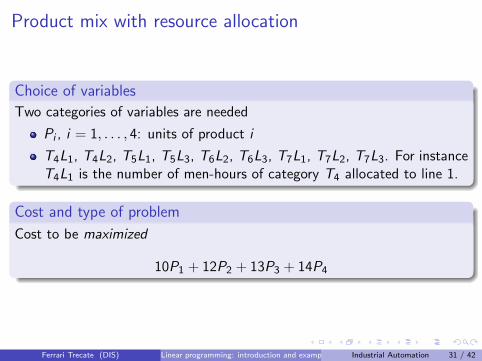
Choice of variables
Two categories of variables are needed
Pi , i = 1, . . . , 4: units of product i
T4L1, T4L2, T5L1, T5L3, T6L2, T6L3, T7L1, T7L2, T7L3. For instanceT4L1 is the number of men-hours of category T4 allocated to line 1.
Cost and type of problem
Cost to be maximized
10P1 + 12P2 + 13P3 + 14P4
Ferrari Trecate (DIS) Linear programming: introduction and examples Industrial Automation 31 / 42

Product mix with resource allocation
ConstraintsCapacity constraints of production lines
2P1 + 2P2 + 3P3 + 3P4 ≤ 12000 + T4L1 + T5L1 + T7L1 (line 1)2P1 + 3P2 + P3 + 2P4 ≤ 7000 + T4L2 + T6L2 + T7L2 (line 2)P1 + 2P2 + 2P3 + 3P4 ≤ 9000 + T5L3 + T6L3 + T7L3 (line 3)
Bounds on the number of products
P2 ≥ 1000P4 ≤ 500
Maximal availability of u.o.w. for versatile workers
T4L1 + T4L2 ≤ 4000T5L1 + T5L3 ≤ 3000T6L2 + T6L3 ≤ 3000T7L1 + T7L2 + T7L3 ≤ 2000
Positivity contraints:P1, P2, P3, P4, T4L1, T4L2, T5L1, T5L3, T6L2, T6L3, T7L1, T7L2, T7L3 ≥ 0
Ferrari Trecate (DIS) Linear programming: introduction and examples Industrial Automation 32 / 42

Product mix with resource allocation
LP problem
max 10P1 + 12P2 + 13P3 + 14P4
2P1 + 2P2 + 3P3 + 3P4 ≤ 12000 + T4L1 + T5L1 + T7L1
2P1 + 3P2 + P3 + 2P4 ≤ 7000 + T4L2 + T6L2 + T7L2
P1 + 2P2 + 2P3 + 3P4 ≤ 9000 + T5L3 + T6L3 + T7L3
P2 ≥ 1000P4 ≤ 500
T4L1 + T4L2 ≤ 4000T5L1 + T5L3 ≤ 3000T6L2 + T6L3 ≤ 3000
T7L1 + T7L2 + T7L3 ≤ 2000P1, P2, P3, P4, T4L1, T4L2, T5L1, T5L3 ≥ 0
T6L2, T6L3, T7L1, T7L2, T7L3 ≥ 0
Exercise
Write the LP problem in matrix notation
Ferrari Trecate (DIS) Linear programming: introduction and examples Industrial Automation 33 / 42

Multiperiod production planning
A company must determine how many washing machines should beproduced during each of the next 5 months. Washing machines productioncan be internal or subcontracted to another company. Productioncapacities and costs are given in the figure
Ferrari Trecate (DIS) Linear programming: introduction and examples Industrial Automation 34 / 42

Multiperiod production planning
Data and Requirements
Inventory cost: 2 Euros/unit for a whole month
Inventory at the beginning of the first month: 300 units
Inventory at the end of the fifth month: 300 units
Demand during each of the next five months (the company must meetdemands on time)
Month Demand
1 12002 21003 24004 30005 4000
How many washing machines must be produced (internally and by thesubcontractor), each month, in order to meet demands on time and minimize thecosts ?
Ferrari Trecate (DIS) Linear programming: introduction and examples Industrial Automation 35 / 42

Multiperiod production planning
Choice of variables
Three categories of variables are needed
Pi , i = 1, . . . , 5: units produced internally during month i
Si , i = 1, . . . , 5: units produced by the subcontrator during month i
Ii , i = 1, . . . , 4: inventory at the end of month i
Cost and type of problem
Cost to be minimized
105∑
i=1
Pi + 155∑
i=1
Si + 24∑
i=1
Ii
Ferrari Trecate (DIS) Linear programming: introduction and examples Industrial Automation 36 / 42

Multiperiod production planning
ConstraintsMaximal production
Pi ≤ 2000, i = 1, . . . , 5 (internal production)Si ≤ 600, i = 1, . . . , 5 (subcontracting)
Balance constraints: for month i ,
Inventory at the end of month i = Inventory at the end of month i − 1 +
+ month i production−month i demand
I1 = 300 + P1 + S1 − 1200I2 = +I1 + P2 + S2 − 2100I3 = +I2 + P2 + S2 − 2400I4 = +I3 + P3 + S3 − 3000300 = +I4 + P4 + S4 − 4000
Positivity contraints: Pi ,Si ≥ 0, i = 1 . . . , 5, Ij ≥ 0, j = 1 . . . , 4
Ferrari Trecate (DIS) Linear programming: introduction and examples Industrial Automation 37 / 42
Multiperiod production planning
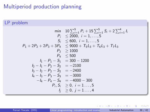
LP problem
min 10∑5
i=1 Pi + 15∑5
i=1 Si + 2∑4
i=1 IiPi ≤ 2000, i = 1, . . . , 5Si ≤ 600, i = 1, . . . , 5
P1 + 2P2 + 2P3 + 3P4 ≤ 9000 + T5L3 + T6L3 + T7L3
P2 ≥ 1000P4 ≤ 500
I1 − P1 − S1 = 300− 1200I2 − I1 − P2 − S2 = −2100I3 − I2 − P2 − S2 = −2400I4 − I3 − P3 − S3 = −3000−I4 − P4 − S4 = −4000− 300
Pi ,Si ≥ 0, i = 1 . . . , 5Ij ≥ 0, j = 1 . . . , 4
Ferrari Trecate (DIS) Linear programming: introduction and examples Industrial Automation 38 / 42

Portfolio optimization
A manager must decide how to invest 500000 Euros in different financialproducts. His goal is to maximize earnings while avoiding high riskexposure
Financial products and expected return on investment
Financial product Market Return %
T1 Cars - Germany 10.3T2 Cars - Japan 10.1T3 Computers - USA 11.8T4 Computers - USA 11.4T5 Household appliances - Europe 12.7T6 Household appliances - Asia 12.2T7 Insurance - Germany 9.5T8 Insurance - USA 9.9T9 BOT 3.6T10 CCT 4.2
Ferrari Trecate (DIS) Linear programming: introduction and examples Industrial Automation 39 / 42

Portfolio optimization
Investment requirements
1 No more than 150000 Euros in the car options2 No more than 150000 Euros in the computer options3 No more than 100000 Euros in the appliance options4 At least 100000 Euros in the insurance options5 At least 125000 Euros in BOT or CCT6 At least 40% of the money invested in CCT must be invested in BOT7 No more than 250000 Euros must be invested in German options8 No more than 200000 Euros must be invested in USA options
Ferrari Trecate (DIS) Linear programming: introduction and examples Industrial Automation 40 / 42
Portfolio optimization
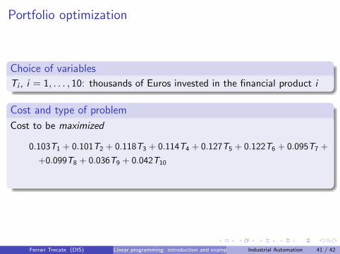
Choice of variables
Ti , i = 1, . . . , 10: thousands of Euros invested in the financial product i
Cost and type of problem
Cost to be maximized
0.103T1 + 0.101T2 + 0.118T3 + 0.114T4 + 0.127T5 + 0.122T6 + 0.095T7 +
+0.099T8 + 0.036T9 + 0.042T10
Ferrari Trecate (DIS) Linear programming: introduction and examples Industrial Automation 41 / 42

Portfolio optimization
Constraints
Total investment:∑10
i=1 Ti = 500Investment requirements:
1 T1 + T2 ≤ 1502 T3 + T4 ≤ 1503 T5 + T6 ≤ 1004 T7 + T8 ≥ 1005 T9 + T10 ≥ 1256 T9 − 0.4T10 ≥ 07 T1 + T7 ≤ 2508 T3 + T4 + T8 ≤ 200
Positivity constraints: Ti ,≥ 0, i = 1 . . . , 10
Ferrari Trecate (DIS) Linear programming: introduction and examples Industrial Automation 42 / 42