g. cowan discovery and limits / desy, 4-7 october 2011 / lecture 1 1 statistical methods for...

G. Cowan Discovery and limits / DESY, 4-7 October 2011 / Lecture 1 1

Statistical Methods for Discovery and Limits

Lecture 1: Introduction, Statistical Tests, Confidence Intervals

School on Data Combination and Limit SettingDESY, 4-7 October, 2011

Glen CowanPhysics DepartmentRoyal Holloway, University of [email protected]/~cowan

http://www.pp.rhul.ac.uk/~cowan/stat_desy.htmlhttps://indico.desy.de/conferenceDisplay.py?confId=4489

http://www.rhul.ac.uk/


Outline

Lecture 1: Introduction and basic formalism Probability, statistical tests, confidence intervals.

Lecture 2: Tests based on likelihood ratios Systematic uncertainties (nuisance parameters)

Lecture 3: Limits for Poisson mean Bayesian and frequentist approaches

Lecture 4: More on discovery and limits Spurious exclusion


Quick review of probablility


Frequentist Statistics − general philosophy In frequentist statistics, probabilities are associated only withthe data, i.e., outcomes of repeatable observations.

Probability = limiting frequency

Probabilities such as

P (Higgs boson exists), P (0.117 < s < 0.121),

etc. are either 0 or 1, but we don’t know which.The tools of frequentist statistics tell us what to expect, underthe assumption of certain probabilities, about hypotheticalrepeated observations.

The preferred theories (models, hypotheses, ...) are those for which our observations would be considered ‘usual’.


Bayesian Statistics − general philosophy In Bayesian statistics, interpretation of probability extended todegree of belief (subjective probability). Use this for hypotheses:

posterior probability, i.e., after seeing the data

prior probability, i.e.,before seeing the data

probability of the data assuming hypothesis H (the likelihood)

normalization involves sum over all possible hypotheses

Bayesian methods can provide more natural treatment of non-repeatable phenomena: systematic uncertainties, probability that Higgs boson exists,...

No golden rule for priors (“if-then” character of Bayes’ thm.)


HypothesesA hypothesis H specifies the probability for the data, i.e., the outcome of the observation, here symbolically: x.

x could be uni-/multivariate, continuous or discrete.

E.g. write x ~ f (x|H).

x could represent e.g. observation of a single particle, a single event, or an entire “experiment”.

Possible values of x form the sample space S (or “data space”).

Simple (or “point”) hypothesis: f (x|H) completely specified.

Composite hypothesis: H contains unspecified parameter(s).

The probability for x given H is also called the likelihood ofthe hypothesis, written L(x|H).


Definition of a testConsider e.g. a simple hypothesis H0 and alternative H1.

A test of H0 is defined by specifying a critical region W of thedata space such that there is no more than some (small) probability, assuming H0 is correct, to observe the data there, i.e.,

P(x W | H0 ) ≤

If x is observed in the critical region, reject H0.

is called the size or significance level of the test.

Critical region also called “rejection” region; complement isacceptance region.


Definition of a test (2)But in general there are an infinite number of possible critical regions that give the same significance level .

So the choice of the critical region for a test of H0 needs to take into account the alternative hypothesis H1.

Roughly speaking, place the critical region where there is a low probability to be found if H0 is true, but high if H1 is true:


Rejecting a hypothesisNote that rejecting H0 is not necessarily equivalent to thestatement that we believe it is false and H1 true. In frequentiststatistics only associate probability with outcomes of repeatableobservations (the data).

In Bayesian statistics, probability of the hypothesis (degreeof belief) would be found using Bayes’ theorem:

which depends on the prior probability (H).

What makes a frequentist test useful is that we can computethe probability to accept/reject a hypothesis assuming that itis true, or assuming some alternative is true.


Type-I, Type-II errors

Rejecting the hypothesis H0 when it is true is a Type-I error.

The maximum probability for this is the size of the test:

P(x W | H0 ) ≤

But we might also accept H0 when it is false, and an alternative H1 is true.

This is called a Type-II error, and occurs with probability

P(x S W | H1 ) =

One minus this is called the power of the test with respect tothe alternative H1:

Power =


Physics context of a statistical testEvent Selection: the event types in question are both known to exist.

Example: separation of different particle types (electron vs muon)or known event types (ttbar vs QCD multijet).Use the selected sample for further study.

Search for New Physics: the null hypothesis H0 means Standard Model events, and the alternative H1 means "events of a type whose existence is not yet established" (to establish or exclude the signal model is the goalof the analysis).

Many subtle issues here, mainly related to the high standardof proof required to establish presence of a new phenomenon.

The optimal statistical test for a search is closely related to that used for event selection.


Suppose we want to discover this…

high pT

muons

high pT jets

of hadrons

missing transverse energy

p p

SUSY event (ATLAS simulation):


But we know we’ll have lots of this…

SM event also has high p

T jets and muons, and

missing transverse energy.

→ can easily mimic a SUSY event and thus constitutes abackground.

ttbar event (ATLAS simulation)


For each reaction we consider we will have a hypothesis for thepdf of , e.g.,

Example of a multivariate statistical testSuppose the result of a measurement for an individual event is a collection of numbers

x1 = number of muons,

x2 = mean pt of jets,

x3 = missing energy, ...

follows some n-dimensional joint pdf, which depends on the type of event produced, i.e., was it

etc.

Often call H0 the background hypothesis (e.g. SM events);H1, H2, ... are possible signal hypotheses.


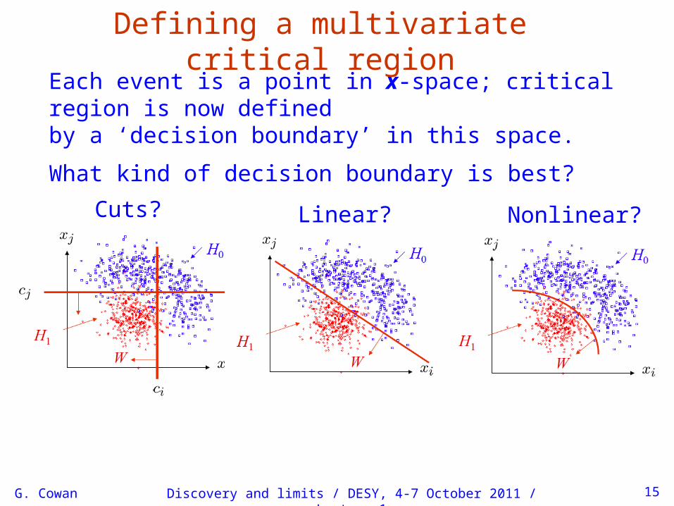
Defining a multivariate critical regionEach event is a point in x-space; critical region is now definedby a ‘decision boundary’ in this space.

What kind of decision boundary is best?

Cuts? Linear? Nonlinear?

G. Cowan Discovery and limits / DESY, 4-7 October 2011 / Lecture 1 Lecture 1 page 16

Multivariate methodsMany new (and some old) methods for finding decision boundary:

Fisher discriminantNeural networksKernel density methodsSupport Vector MachinesDecision trees

BoostingBagging

New software for HEP, e.g.,

TMVA , Höcker, Stelzer, Tegenfeldt, Voss, Voss, physics/0703039

For more see e.g. references at end of this lecture.

For the rest of these lectures, I will focus on other aspects of tests, e.g., discovery significance and exclusion limits.


Test statisticsThe decision boundary can be defined by an equation of the form

We can work out the pdfs

Decision boundary is now a single ‘cut’ on t, defining the critical region.

So for an n-dimensional problem we have a corresponding 1-d problem.

where t(x1,…, xn) is a scalar test statistic.


Significance level and power

Probability to reject H0 if it is true (type-I error):

(significance level)

Probability to accept H0 if H1 is true (type-II error):

( power)


Constructing a test statisticHow can we choose a test’s critical region in an ‘optimal way’?

Neyman-Pearson lemma states:

To get the highest power for a given significance level in a testH0, (background) versus H1, (signal) (highest s for a given b)choose the critical (rejection) region such that

where c is a constant which determines the power.

Equivalently, optimal scalar test statistic is

N.B. any monotonic function of this is leads to the same test.


Testing significance / goodness-of-fit

Suppose hypothesis H predicts pdf

observations

for a set of

We observe a single point in this space:

What can we say about the validity of H in light of the data?

Decide what part of the data space represents less compatibility with H than does the point less

compatiblewith H

more compatiblewith H

(Not unique!)


p-values

where (H) is the prior probability for H.

Express level of agreement between data and H with p-value:

p = probability, under assumption of H, to observe data with equal or lesser compatibility with H relative to the data we got.

This is not the probability that H is true!

In frequentist statistics we don’t talk about P(H) (unless H represents a repeatable observation). In Bayesian statistics we do; use Bayes’ theorem to obtain

For now stick with the frequentist approach; result is p-value, regrettably easy to misinterpret as P(H).

G. Cowan 22

Significance from p-value

Often define significance Z as the number of standard deviationsthat a Gaussian variable would fluctuate in one directionto give the same p-value.

1 - TMath::Freq

TMath::NormQuantile

Discovery and limits / DESY, 4-7 October 2011 / Lecture 1


The significance of an observed signalSuppose we observe n events; these can consist of:

nb events from known processes (background)ns events from a new process (signal)

If ns, nb are Poisson r.v.s with means s, b, then n = ns + nb

is also Poisson, mean = s + b:

Suppose b = 0.5, and we observe nobs = 5. Should we claimevidence for a new discovery?

Give p-value for hypothesis s = 0:

G. Cowan page 24

Distribution of the p-valueThe p-value is a function of the data, and is thus itself a randomvariable with a given distribution. Suppose the p-value of H is found from a test statistic t(x) as


The pdf of pH under assumption of H is

In general for continuous data, under assumption of H, pH ~ Uniform[0,1]and is concentrated toward zero for some (broad) class of alternatives. pH

g(pH|H)

0 1

g(pH|H′)

G. Cowan page 25

Using a p-value to define test of H0

So the probability to find the p-value of H0, p0, less than is


We started by defining critical region in the original dataspace (x), then reformulated this in terms of a scalar test statistic t(x).

We can take this one step further and define the critical region of a test of H0 with size as the set of data space where p0 ≤ .

Formally the p-value relates only to H0, but the resulting test willhave a given power with respect to a given alternative H1.


Interval estimation — introduction

Often use +/ the estimated standard deviation of the estimator.In some cases, however, this is not adequate:

estimate near a physical boundary, e.g., an observed event rate consistent with zero.

In addition to a ‘point estimate’ of a parameter we should report an interval reflecting its statistical uncertainty.

Desirable properties of such an interval may include:communicate objectively the result of the experiment;have a given probability of containing the true parameter;provide information needed to draw conclusions aboutthe parameter possibly incorporating stated prior beliefs.

We will look briefly at Frequentist and Bayesian intervals.


Frequentist confidence intervals

Consider an estimator for a parameter and an estimate

We also need for all possible its sampling distribution

Specify upper and lower tail probabilities, e.g., = 0.05, = 0.05,then find functions u() and v() such that:


Confidence interval from the confidence belt

Find points where observed estimate intersects the confidence belt.

The region between u() and v() is called the confidence belt.

This gives the confidence interval [a, b]

Confidence level = 1 = probability for the interval tocover true value of the parameter (holds for any possible true ).


Confidence intervals by inverting a test

Confidence intervals for a parameter can be found by defining a test of the hypothesized value (do this for all ):

Specify values of the data that are ‘disfavoured’ by (critical region) such that P(data in critical region) ≤ for a prespecified , e.g., 0.05 or 0.1.

If data observed in the critical region, reject the value .

Now invert the test to define a confidence interval as:

set of values that would not be rejected in a test ofsize (confidence level is 1 ).

The interval will cover the true value of with probability ≥ 1 .

Equivalent to confidence belt construction; confidence belt is acceptance region of a test.

Discovery and limits / DESY, 4-7 October 2011 / Lecture 1 30

Relation between confidence interval and p-value

Equivalently we can consider a significance test for eachhypothesized value of , resulting in a p-value, p..

If p < , then we reject .

The confidence interval at CL = 1 – consists of those values of that are not rejected.

E.g. an upper limit on is the greatest value for which p ≥

In practice find by setting p = and solve for .

G. Cowan


Meaning of a confidence interval


Test statistic for p-value of a parameter

One often obtains the p-value of a hypothesized value of a parameter θ using a test statistic qθ(x), such that large values of qθ correspond to increasing incompatibility between the data (x) and hypothesis (θ).

The data result in a value qθ,obs.

The p-value of the hypothesized θ is therefore

So to find this we need to know the distribution of qθ

under assumption of θ.

For some problems we can write this down in closed form (atleast approximately); other times need Monte Carlo.


Nuisance parametersIn general our model of the data is not perfect:

x

L (

x|θ)

model:

truth:

Can improve model by including additional adjustable parameters.

Nuisance parameter ↔ systematic uncertainty. Some point in theparameter space of the enlarged model should be “true”.

Presence of nuisance parameter decreases sensitivity of analysisto the parameter of interest (e.g., increases variance of estimate).


Distribution of qθ in case of nuisance parameters

The p-value of θ is now

But what values of ν to use for f (qθ|θ, ν)?

Fundamentally we want to reject θ only if pθ < α for all ν.

→ “exact” confidence interval

We will see that for certain statistics (based on the profile likelihood ratio), the distribution f (qθ|θ, ν) becomes independent of the nuisance parameters in the large-sample limit.

But in general for finite data samples this is not true; may be unable to reject some θ values if ν is assumed equal to some value that is strongly disfavoured by the data (resulting interval for θ “overcovers”).


Profile construction (“hybrid resampling”)

Compromise procedure is to reject θ if pθ < α wherethe p-value is computed assuming the value of the nuisanceparameter that best fits the data for the specified θ:

“double hat” notation meansvalue of parameter that maximizeslikelihood for the given θ.

The resulting confidence interval will have the correct coveragefor the points (, ˆ̂ν()) .

Elsewhere it may under- or overcover, but this is usually as goodas we can do (check with MC if crucial).


“Hybrid frequentist-Bayesian” method

Alternatively, suppose uncertainty in ν is characterized bya Bayesian prior π(ν).

Can use the marginal likelihood to model the data:

This does not represent what the data distribution wouldbe if we “really” repeated the experiment, since then ν wouldnot change.

But the procedure has the desired effect. The marginal likelihoodeffectively builds the uncertainty due to ν into the model.

Use this now to compute (frequentist) p-values → resulthas hybrid “frequentist-Bayesian” character.


The “ur-prior” behind the hybrid method

But where did π(ν) come frome? Presumably at some earlierpoint there was a measurement of some data y withlikelihood L(y|ν), which was used in Bayes’theorem,

and this “posterior” was subsequently used for π(ν) for thenext part of the analysis.

But it depends on an “ur-prior” π0(ν), which still has to bechosen somehow (perhaps “flat-ish”).

But once this is combined to form the marginal likelihood, theorigin of the knowledge of ν may be forgotten, and the modelis regarded as only describing the data outcome x.


The (pure) frequentist equivalent

In a purely frequentist analysis, one would regard bothx and y as part of the data, and write down the full likelihood:

“Repetition of the experiment” here means generating bothx and y according to the distribution above.

In many cases, the end result from the hybrid and purefrequentist methods are found to be very similar (cf. Conway,Roever, PHYSTAT 2011).


Wrapping up lecture 1

General framework of a statistical test:Divide data spaced into two regions; depending onwhere data are then observed, accept or reject hypothesis.

Significance tests (also for goodness-of-fit):p-value = probability to see level of incompatibilitybetween data and hypothesis equal to or greater thanlevel found with the actual data.

Confidence intervalsSet of parameter values not rejected in a test of sizeα gives confidence interval at 1 – α CL.

Systematic uncertainties ↔ nuisance parameters


Extra slides


Signal/background efficiency

Probability to reject background hypothesis for background event (background efficiency):

Probability to accept a signal eventas signal (signal efficiency):


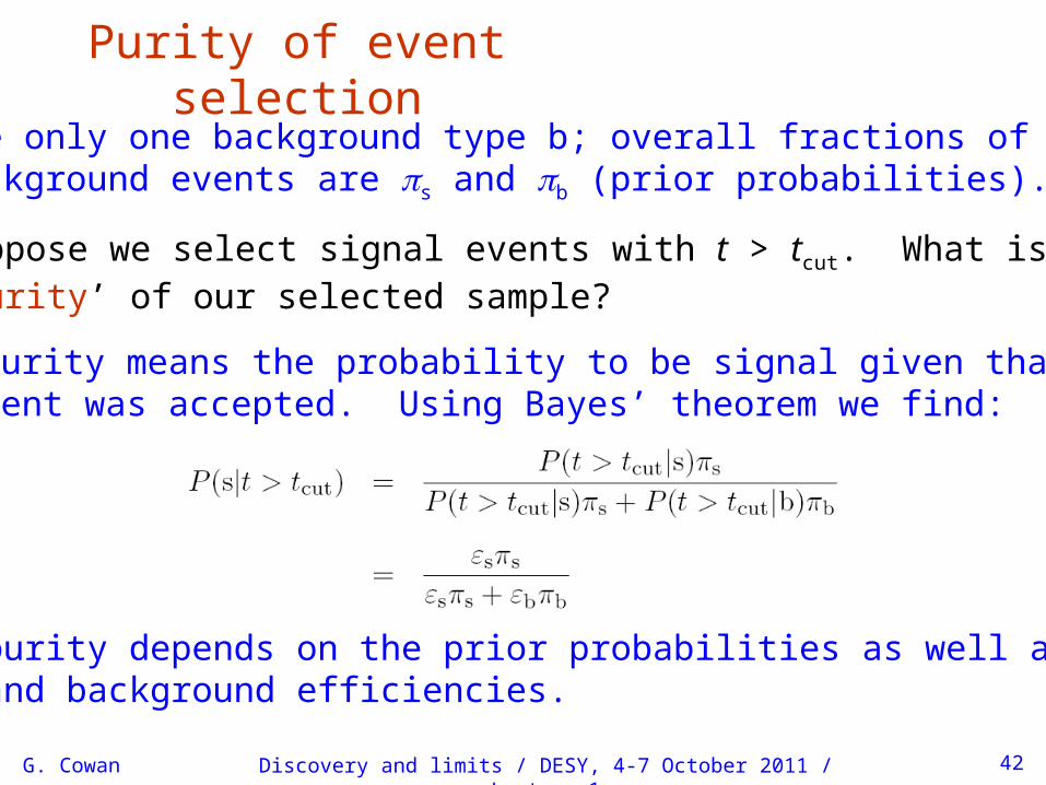
Purity of event selectionSuppose only one background type b; overall fractions of signaland background events are s and b (prior probabilities).

Suppose we select signal events with t > tcut. What is the‘purity’ of our selected sample?

Here purity means the probability to be signal given thatthe event was accepted. Using Bayes’ theorem we find:

So the purity depends on the prior probabilities as well as on thesignal and background efficiencies.


Proof of Neyman-Pearson lemma

We want to determine the critical region W that maximizes the power

subject to the constraint

First, include in W all points where P(x|H0) = 0, as they contributenothing to the size, but potentially increase the power.


Proof of Neyman-Pearson lemma (2)

For P(x|H0) ≠ 0 we can write the power as

The ratio of 1 – to is therefore

which is the average of the likelihood ratio P(x|H1) / P(x|H0) overthe critical region W, assuming H0.

(1 – ) / is thus maximized if W contains the part of the samplespace with the largest values of the likelihood ratio.


p-value example: testing whether a coin is ‘fair’

i.e. p = 0.0026 is the probability of obtaining such a bizarreresult (or more so) ‘by chance’, under the assumption of H.

Probability to observe n heads in N coin tosses is binomial:

Hypothesis H: the coin is fair (p = 0.5).

Suppose we toss the coin N = 20 times and get n = 17 heads.

Region of data space with equal or lesser compatibility with H relative to n = 17 is: n = 17, 18, 19, 20, 0, 1, 2, 3. Addingup the probabilities for these values gives:


Quick review of parameter estimationThe parameters of a pdf are constants that characterize its shape, e.g.

random variable

Suppose we have a sample of observed values:

parameter

We want to find some function of the data to estimate the parameter(s):

← estimator written with a hat

Sometimes we say ‘estimator’ for the function of x1, ..., xn;‘estimate’ for the value of the estimator with a particular data set.


The likelihood functionSuppose the entire result of an experiment (set of measurements)is a collection of numbers x, and suppose the joint pdf forthe data x is a function that depends on a set of parameters :

Now evaluate this function with the data obtained andregard it as a function of the parameter(s). This is the likelihood function:

(x constant)


The likelihood function for i.i.d.*. data

Consider n independent observations of x: x1, ..., xn, where x follows f (x; ). The joint pdf for the whole data sample is:

In this case the likelihood function is

(xi constant)

* i.i.d. = independent and identically distributed


Maximum likelihood estimatorsIf the hypothesized is close to the true value, then we expect a high probability to get data like that which we actually found.

So we define the maximum likelihood (ML) estimator(s) to be the parameter value(s) for which the likelihood is maximum.

ML estimators not guaranteed to have any ‘optimal’properties, (but in practice they’re very good).


ML example: parameter of exponential pdf

Consider exponential pdf,

and suppose we have i.i.d. data,

The likelihood function is

The value of for which L() is maximum also gives the maximum value of its logarithm (the log-likelihood function):


ML example: parameter of exponential pdf (2)

Find its maximum by setting

→

Monte Carlo test: generate 50 valuesusing = 1:

We find the ML estimate:


Variance of estimators from information inequalityThe information inequality (RCF) sets a lower bound on the variance of any estimator (not only ML):

Often the bias b is small, and equality either holds exactly oris a good approximation (e.g. large data sample limit). Then,

Estimate this using the 2nd derivative of ln L at its maximum:


Information inequality for n parametersSuppose we have estimated n parameters

The (inverse) minimum variance bound is given by the Fisher information matrix:

The information inequality then states that V I is a positivesemi-definite matrix, where Therefore

Often use I as an approximation for covariance matrix, estimate using e.g. matrix of 2nd derivatives at maximum of L.


Extended MLSometimes regard n not as fixed, but as a Poisson r.v., mean ν.

Result of experiment defined as: n, x1, ..., xn.

The (extended) likelihood function is:

Suppose theory gives ν = ν(), then the log-likelihood is

where C represents terms not depending on .


Extended ML (2)

Extended ML uses more info → smaller errors for

Example: expected number of events

where the total cross section () is predicted as a function of

the parameters of a theory, as is the distribution of a variable x.

If ν does not depend on but remains a free parameter,extended ML gives:

Important e.g. for anomalous couplings in ee → W+W


Extended ML exampleConsider two types of events (e.g., signal and background) each of which predict a given pdf for the variable x: fs(x) and fb(x).

We observe a mixture of the two event types, signal fraction = , expected total number = ν, observed total number = n.

Let goal is to estimate s, b.

→


Extended ML example (2)

Maximize log-likelihood in terms of s and b:

Monte Carlo examplewith combination ofexponential and Gaussian:

Here errors reflect total Poissonfluctuation as well as that in proportion of signal/background.


Extended ML example: an unphysical estimate

A downwards fluctuation of data in the peak region can leadto even fewer events than what would be obtained frombackground alone.

Estimate for s here pushednegative (unphysical).

We can let this happen as long as the (total) pdf stayspositive everywhere.


Unphysical estimators (2)

Here the unphysical estimator is unbiased and should nevertheless be reported, since average of a large number of unbiased estimates converges to the true value (cf. PDG).

Repeat entire MCexperiment many times, allow unphysical estimates:

G. Cowan Discovery and limits / DESY, 4-7 October 2011 / Lecture 1 page 60

G. Cowan Discovery and limits / DESY, 4-7 October 2011 / Lecture 1 page 61

g. cowan discovery and limits / desy, 4-7 october 2011 / lecture 1 1 statistical methods for...

Documents