G-CNN: an Iterative Grid Based Object Detector

Mahyar Najibi Mohammad Rastegari Larry S. Davis

University of Maryland, College Park

{najibi,mrastega}@cs.umd.edu lsd@umiacs.umd.edu

Abstract

We introduce G-CNN, an object detection technique

based on CNNs which works without proposal algorithms.

G-CNN starts with a multi-scale grid of fixed bounding

boxes. We train a regressor to move and scale elements

of the grid towards objects iteratively. G-CNN models the

problem of object detection as finding a path from a fixed

grid to boxes tightly surrounding the objects. G-CNN with

around 180 boxes in a multi-scale grid performs compara-

bly to Fast R-CNN which uses around 2K bounding boxes

generated with a proposal technique. This strategy makes

detection faster by removing the object proposal stage as

well as reducing the number of boxes to be processed.

1. Introduction

Object detection, i.e. the problem of finding the locations

of objects and determining their categories, is an intrinsi-

cally more challenging problem than classification since it

includes the problem of object localization. The recent and

popular trend in object detection uses a pre-processing step

to find a candidate set of bounding-boxes that are likely to

encompass the objects in the image. This step is referred

to as the bounding-box proposal stage. The proposal tech-

niques are a major computational bottleneck in state-of-the-

art object detectors [6]. There have been attempts [16, 14]

to take this pre-processing stage out of the loop but they

lead to performance degradations.

We show that without object proposals, we can achieve

detection rates similar to state-of-the-art performance in ob-

ject detection. Inspired by the iterative optimization in [2],

we introduce an iterative algorithm that starts with a reg-

ularly sampled multi-scale grid of boxes in an image and

updates the boxes to cover and classify objects. One step

regression can-not handle the non-linearity of the mapping

from a regular grid to boxes containing objects. Instead, we

introduce a piecewise regression model that can learn this

non-linear mapping through a few iterations. Each step in

our algorithm deals with an easier regression problem than

enforcing a direct mapping to actual target locations.

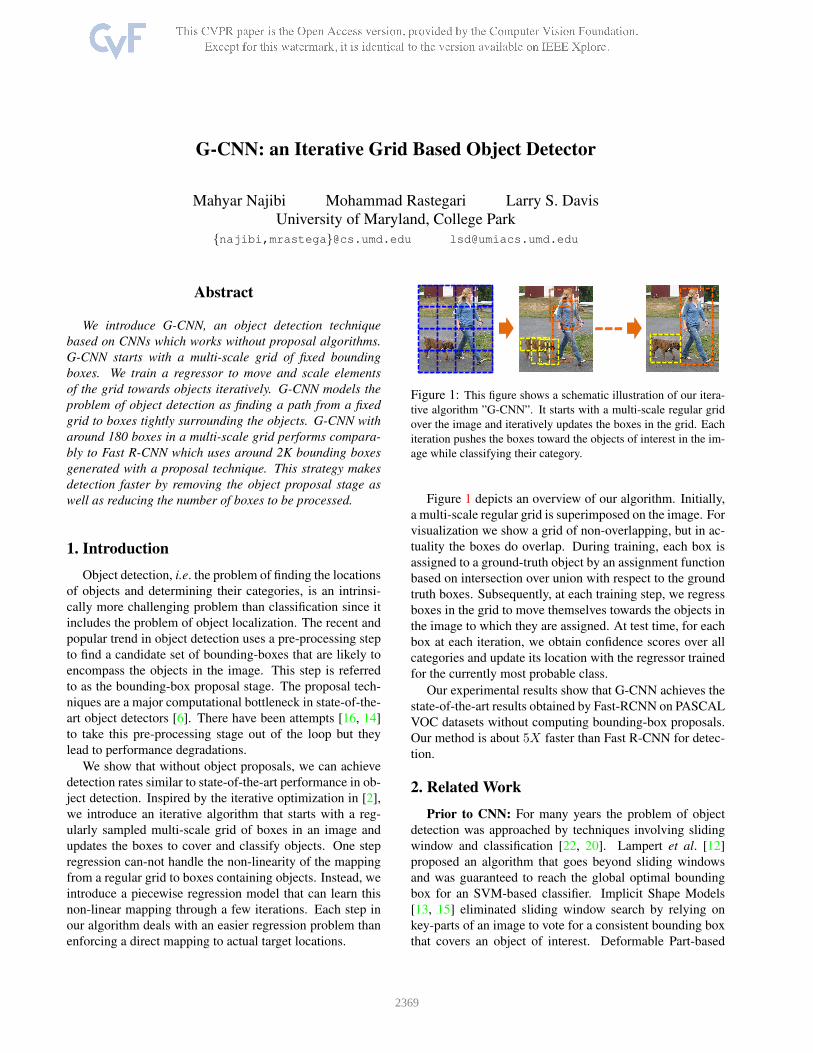
Figure 1: This figure shows a schematic illustration of our itera-

tive algorithm ”G-CNN”. It starts with a multi-scale regular grid

over the image and iteratively updates the boxes in the grid. Each

iteration pushes the boxes toward the objects of interest in the im-

age while classifying their category.

Figure 1 depicts an overview of our algorithm. Initially,

a multi-scale regular grid is superimposed on the image. For

visualization we show a grid of non-overlapping, but in ac-

tuality the boxes do overlap. During training, each box is

assigned to a ground-truth object by an assignment function

based on intersection over union with respect to the ground

truth boxes. Subsequently, at each training step, we regress

boxes in the grid to move themselves towards the objects in

the image to which they are assigned. At test time, for each

box at each iteration, we obtain confidence scores over all

categories and update its location with the regressor trained

for the currently most probable class.

Our experimental results show that G-CNN achieves the

state-of-the-art results obtained by Fast-RCNN on PASCAL

VOC datasets without computing bounding-box proposals.

Our method is about 5X faster than Fast R-CNN for detec-

tion.

2. Related Work

Prior to CNN: For many years the problem of object

detection was approached by techniques involving sliding

window and classification [22, 20]. Lampert et al. [12]

proposed an algorithm that goes beyond sliding windows

and was guaranteed to reach the global optimal bounding

box for an SVM-based classifier. Implicit Shape Models

[13, 15] eliminated sliding window search by relying on

key-parts of an image to vote for a consistent bounding box

that covers an object of interest. Deformable Part-based

2369

Models [4] employed an idea similar to Implicit Shape

Models, but proposed a direct optimization via latent vari-

able models and used dynamic programming for fast infer-

ence. Several extension of DPMs emerged [5, 1] until the

remarkable improvements due to the convolutional neural

networks was shown by [7].

CNN age: Deep convolutional neural networks (CNNs)

are the state-of-the-art image classifiers and successful

methods have been proposed based on these networks [11].

Driven by their success in image classification, Girshick et

al. proposed a multi-stage object detection system, known

as R-CNN [7], which has attracted great attention due to its

success on standard object detection datasets.

To address the localization problem, R-CNN relies on

advances in object proposal techniques. Recently, proposal

algorithms have been developed which avoid exhaustive

search of image locations [21, 24]. R-CNN uses these tech-

niques to find bounding boxes which include an object with

high probability. Next, a standard CNN is applied as fea-

ture extractor to each proposed bounding box and finally a

classifier decides which object class is inside the box.

The main drawback of R-CNN is the redundancy in com-

puting the features. Generally, around 2K proposals are

generated; for each of them, the CNN is applied indepen-

dently to extract features. To alleviate this problem, in SPP-

Net [9] the convolutional layers of the network are applied

only once for each image. Then, the features of each region

of interest are constructed by pooling the global features

which lie in the spatial support of the region. However,

learning is limited to fine-tuning the weights of fully con-

nected layers. This drawback is addressed in Fast-RCNN

[6] in which all parameters are learned by back propagating

the errors through the augmented pooling layer and pack-

ing all stages of the system, except generation of the object

proposals, into one network.

The generation of object proposals, in CNN-based de-

tection systems has been regarded as crucial. However, after

proposing Fast-RCNN, this stage became the bottleneck. To

make the number of object proposals smaller, Multibox[3]

introduced a proposal algorithm that outputs 800 bounding

boxes using a CNN. This increases the size of the final layer

of the CNN to 4096x800x5 and introduces a large set of ad-

ditional parameters. Recently, Faster-RCNN [17] was pro-

posed, which decreased the number of parameters; however

it needs to start from thousands of anchor points to propose

300 boxes.

In addition to classification, using a regressor for object

detection has been also studied previously. Before propos-

ing R-CNN, Szegedy et al. [19], modeled object detection

as a regression problem and proposed a CNN-based regres-

sion system. More recently, AttentionNet [23] is a single

category detection that detects a single object inside an im-

age using iterative regression. For multiple objects, the

model is applied as a proposal algorithm to generate thou-

sands of proposals and then is re-applied iteratively on each

proposal for single category detection, which makes detec-

tion inefficient.

Although R-CNN and its variants attack the problem us-

ing a classification approach, they employ regression as a

post-processing stage to refine the localization of the pro-

posed bounding boxes.

The importance of the regression stage has not received

as much attention as improving the object proposal stage

for more accurate localization. The necessity of an object

proposal algorithm in CNN based object detection systems

has recently been challenged by Lenc et al. [14]. Here, the

proposals are replaced by a fixed set of bounding boxes.

A set with a distribution derived from an object proposal

method is selected using a clustering technique. However,

for achieving comparable results, even more boxes need to

be used compared to R-CNN. Another recent attempt for re-

moving the proposal stage is Redmon et al. [16] which con-

ducts object detection in a single shot. However, the consid-

erable gap between the best detection accuracy of these sys-

tems and systems with an explicit proposal stage suggests

that the identification of good object proposals is critical to

the success of these CNN based detection systems.

3. G-CNN Object Detector

3.1. Network structure

G-CNN trains a CNN to move and scale a fixed multi-

scale grid of bounding boxes towards objects. The network

architecture for this regressor is shown in Figure 2. The

backbone of this architecture can be any CNN network (e.g.

AlexNet [11], VGG [18], etc.). As in Fast R-CNN and

SPP-Net, a spatial region of interest (ROI) pooling layer

is included in the architecture after the convolutional lay-

ers. Given the location information of each box, this layer

computes the feature for the box by pooling the global fea-

tures that lie inside the ROI. After the fully connected lay-

ers, the network ends with a linear regressor which outputs

the change in the location and scale of each current bound-

ing box, conditioned on the assumption that the box is mov-

ing towards an object of a class.

3.2. Training the network

Despite the similarities between the Fast R-CNN and G-

CNN architectures, the training goals and approaches are

different. G-CNN defines the problem of object detection

as an iterative search in the space of all possible bound-

ing boxes. G-CNN starts from a fixed multi-scale spatial

pyramid of boxes. The goal of learning is to train the net-

work so that it can move this set of initial boxes towards

the objects inside the image in S steps iteratively. This it-

erative behaviour is essential for the success of the algo-

2370

Convolu'onal

Layers

ROI Pooling 

FC

Layers

Cla

ss

-wis

ed

Re

gre

ss

or

Update Position of Bounding Box

Bounding box and its

target at step t (Bs,Ts)

Update the target bounding box

G-CNN Network Structure

(Bs+1) (Bs+1,Ts+1)

Next Step

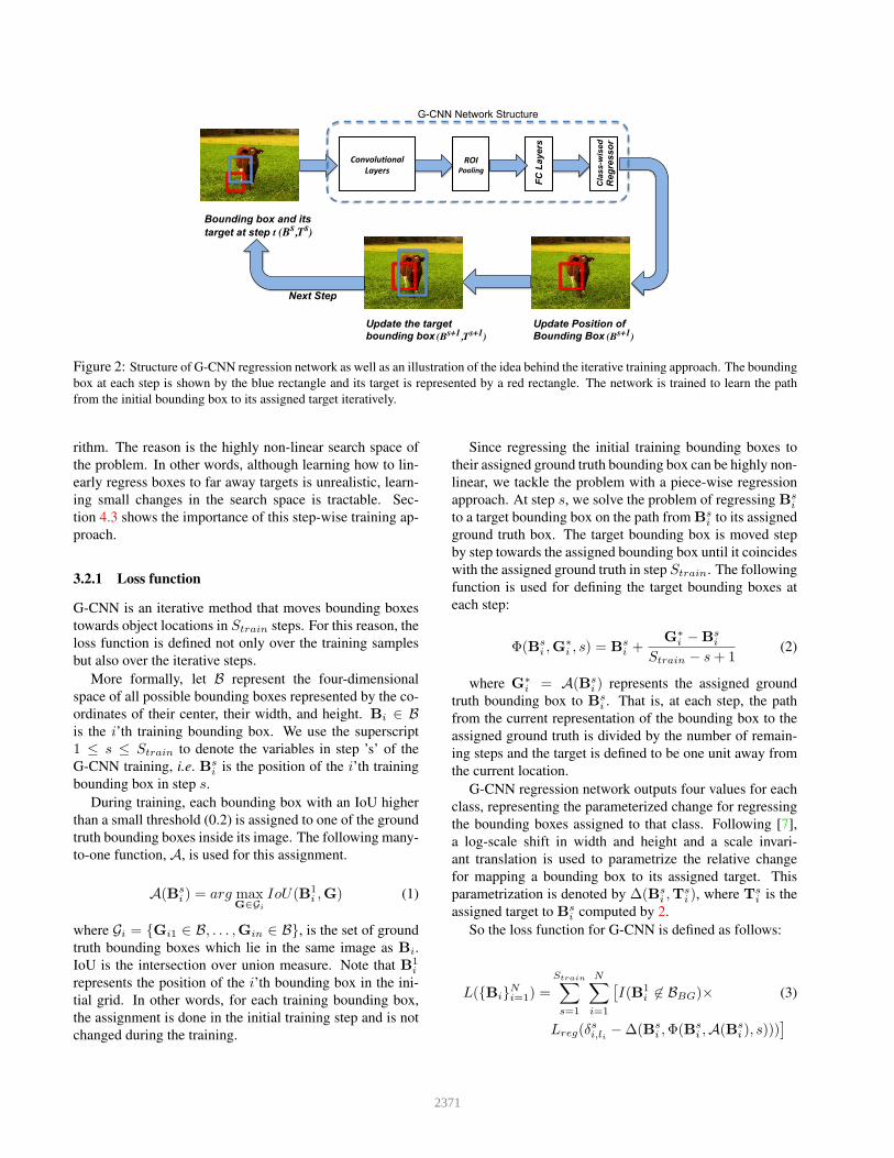
Figure 2: Structure of G-CNN regression network as well as an illustration of the idea behind the iterative training approach. The bounding

box at each step is shown by the blue rectangle and its target is represented by a red rectangle. The network is trained to learn the path

from the initial bounding box to its assigned target iteratively.

rithm. The reason is the highly non-linear search space of

the problem. In other words, although learning how to lin-

early regress boxes to far away targets is unrealistic, learn-

ing small changes in the search space is tractable. Sec-

tion 4.3 shows the importance of this step-wise training ap-

proach.

3.2.1 Loss function

G-CNN is an iterative method that moves bounding boxes

towards object locations in Strain steps. For this reason, the

loss function is defined not only over the training samples

but also over the iterative steps.

More formally, let B represent the four-dimensional

space of all possible bounding boxes represented by the co-

ordinates of their center, their width, and height. Bi ∈ Bis the i’th training bounding box. We use the superscript

1 ≤ s ≤ Strain to denote the variables in step ’s’ of the

G-CNN training, i.e. Bsi is the position of the i’th training

bounding box in step s.

During training, each bounding box with an IoU higher

than a small threshold (0.2) is assigned to one of the ground

truth bounding boxes inside its image. The following many-

to-one function, A, is used for this assignment.

A(Bsi ) = arg max

G∈Gi

IoU(B1i ,G) (1)

where Gi = {Gi1 ∈ B, . . . ,Gin ∈ B}, is the set of ground

truth bounding boxes which lie in the same image as Bi.

IoU is the intersection over union measure. Note that B1i

represents the position of the i’th bounding box in the ini-

tial grid. In other words, for each training bounding box,

the assignment is done in the initial training step and is not

changed during the training.

Since regressing the initial training bounding boxes to

their assigned ground truth bounding box can be highly non-

linear, we tackle the problem with a piece-wise regression

approach. At step s, we solve the problem of regressing Bsi

to a target bounding box on the path from Bsi to its assigned

ground truth box. The target bounding box is moved step

by step towards the assigned bounding box until it coincides

with the assigned ground truth in step Strain. The following

function is used for defining the target bounding boxes at

each step:

Φ(Bsi ,G

∗i , s) = B

si +

G∗i −B

si

Strain − s+ 1(2)

where G∗i = A(Bs

i ) represents the assigned ground

truth bounding box to Bsi . That is, at each step, the path

from the current representation of the bounding box to the

assigned ground truth is divided by the number of remain-

ing steps and the target is defined to be one unit away from

the current location.

G-CNN regression network outputs four values for each

class, representing the parameterized change for regressing

the bounding boxes assigned to that class. Following [7],

a log-scale shift in width and height and a scale invari-

ant translation is used to parametrize the relative change

for mapping a bounding box to its assigned target. This

parametrization is denoted by ∆(Bsi ,T

si ), where T

si is the

assigned target to Bsi computed by 2.

So the loss function for G-CNN is defined as follows:

L({Bi}Ni=1) =

Strain∑

s=1

N∑

i=1

[

I(B1i 6∈ BBG)× (3)

Lreg(δsi,li−∆(Bs

i ,Φ(Bsi ,A(B

si ), s)))

]

2371

where δsi,li is the four-dimensional parameterized output

for class li representing the relative change in the represen-

tation of bounding box Bsi . li is the class label of the as-

signed ground truth bounding box to Bi. Lreg is the regres-

sion loss function. The smooth l1 loss is used as defined in

[6]. I(.) is the indicator function which outputs one when

its condition is satisfied and zero otherwise. BBG represents

the set of all background bounding boxes.

During training, the representation of bounding box Bi

at step s, Bsi , can be determined based on the actual output

of the network by the following update formula:

Bsi = B

s−1

i +∆−1(δs−1

i,li) (4)

where ∆−1 projects back the relative change in the posi-

tion and scale from the defined parametrized space into B.

However for calculating 4, the forward path of the network

needs to be evaluated during training, making training inef-

ficient. Instead, we use an approximate update by assuming

that in step s, the network could learn the regressor for step

s − 1 perfectly. As a result the update formula becomes

Bsi = Φ(Bs−1

i ,G∗i , s− 1). This update is depicted in Fig-

ure 2.

3.2.2 Optimization

G-CNN optimizes the objective function in 3 with stochas-

tic gradient descent. Since G-CNN tries to map the bound-

ing boxes to their assigned ground-truth boxes in Strain

steps, we use a step-wised learning algorithm that optimizes

Eq. 3 step by step.

To this end, we treat each of the bounding boxes in the

initial grid together with its target in each of the steps as an

independent training sample i.e. for each of the bounding

boxes we have Strain different training pairs. The algorithm

first tries to optimize the loss function for the first step using

Niter iterations. Then the training pairs of the second step

are added to the training set and training continues step by

step. By keeping the samples of the previous steps in the

training set, we make sure that the network does not forget

what was learned in the previous steps.

The samples for the earlier steps are part of the training

set for a longer period of time. This choice is made since the

earlier steps determine the global search direction and have

a greater impact on the chance that the network will find

the objects. On the other hand, the later steps only refine

the bounding boxes to decrease localization error. Given

that the search direction was correct and a good part of the

object is now visible in the bounding box, the later steps

solve a relatively easier problem.

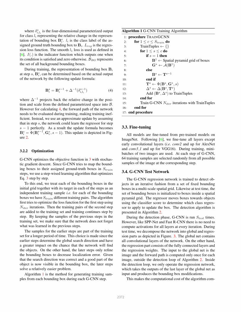
Algorithm 1 is the method for generating training sam-

ples from each bounding box during each G-CNN step.

Algorithm 1 G-CNN Training Algorithm

1: procedure TRAINGCNN

2: for 1 ≤ c ≤ Strain do

3: TrainTuples← {}4: for 1 ≤ s ≤ c do

5: if s = 1 then

6: B1 ← Spatial pyramid grid of boxes

7: G∗ ← A(B1)

8: else

9: Bs ← T

s−1

10: end if

11: Ts ← Φ(Bs,G∗, s)

12: ∆s ← ∆(Bs,Ts)13: Add (Bs,∆s) to TrainTuples

14: end for

15: Train G-CNN Niter iterations with TrainTuples

16: end for

17: end procedure

3.3. Fine­tuning

All models are fine-tuned from pre-trained models on

ImageNet. Following [6], we fine-tune all layers except

early convolutional layers (i.e. conv2 and up for AlexNet

and conv3 1 and up for VGG16). During training, mini-

batches of two images are used. At each step of G-CNN,

64 training samples are selected randomly from all possible

samples of the image at the corresponding step.

3.4. G­CNN Test Network

The G-CNN regression network is trained to detect ob-

jects in an iterative fashion from a set of fixed bounding

boxes in a multi-scale spatial grid. Likewise at test time, the

set of bounding boxes is initialized to boxes inside a spatial

pyramid grid. The regressor moves boxes towards objects

using the classifier score to determine which class regres-

sor to apply to update the box. The detection algorithm is

presented in Algorithm 2.

During the detection phase, G-CNN is run Stest times.

However, like SPP-Net and Fast R-CNN there is no need to

compute activations for all layers at every iteration. During

test time, we decompose the network into global and regres-

sion parts as depicted in Figure. 3. The global net contains

all convolutional layers of the network. On the other hand,

the regression part consists of the fully connected layers and

the regression weights. The input to the global net is the

image and the forward path is computed only once for each

image, outside the detection loop of Algorithm 2. Inside

the detection loop, we only operate the regression network,

which takes the outputs of the last layer of the global net as

input and produces the bounding box modifications.

This makes the computational cost of the algorithm com-

2372

Conv

Layers

Global Part

ROI

POOL

Reg

ress

or

ROI

INFO

Conv

Output

Regression PartF

C L

ayer

s

Modifi

cati

on

In

fo

Figure 3: Decomposition of the G-CNN network into global (up-

per) and regression part (lower) for detection after the training

phase. Global part is run only once to extract global features but

regression part is run at every iteration. This leads to a consider-

able speed up at test time.

parable to Fast R-CNN (without considering the object pro-

posal stage of Fast R-CNN). The global net is called once

in both Fast R-CNN and G-CNN. Afterward, Fast R-CNN

does Nproposal forward calculations of the regression net-

work (where Nproposal is the number of generated object

proposals for each image). G-CNN, on the other hand, does

this forward calculation Stest × Ngrid times (where Ngrid

is the number of bounding boxes in the initial grid). In sec-

tion 4.2, we show that for Stest = 5 and Ngrid ∼ 180,

G-CNN achieves comparable results to Fast R-CNN which

uses Nproposal ∼ 2K object proposals.

4. Experiments

4.1. Experimental Setup

We report results on the Pascal VOC 2007 and Pascal

VOC 2012 datasets. The performance of G-CNN is evalu-

ated with AlexNet [11] as a small and VGG16 [18] as a very

deep CNN structure. Following [7], we scale the shortest

side of the image to 600 pixels not allowing the longer side

of the image to be more than 1000 pixels. However, we al-

ways maintain the aspect ratio of the image, so the shortest

side might include fewer than 600 pixels. Each model is

Algorithm 2 Detection algorithm

1: Let f(.) be the feed-forward G-CNN regression network

2: Let c(.) be the classifier function

3: procedure DETECT

4: B1 ← Spatial pyramid grid of boxes

5: for 1 ≤ s ≤ Stest do

6: l← c(Bs)7: δsl ← f(Bs)8: B

s+1 ← Bs +∆−1(δsl )

9: end for

10: Output BStest+1

11: end procedure

pre-trained with weights learned from the imagenet dataset.

In all the experiments, the G-CNN regression network

is trained on an initial overlapping spatial pyramid with

[2,5,10] scales (i.e. the bounding boxes in the coarsest level

are (imwidth/2, imheight/2) pixels etc.). During training,

we used [0.9,0.8,0.7] overlap for each spatial scale respec-

tively. By overlap of α we mean that the horizontal and

vertical strides are widthcell ∗ (1 − α) and heightcell ∗(1 − α) respectively. However, during test time, as will

be shown in the following sections, overlaps of [0.7,0.5,0]

(non-overlapping grid at the finest scale) is sufficient to ob-

tain results comparable to Fast R-CNN. This leads to a grid

of almost 180 initial boxes at test time. The G-CNN regres-

sion network is trained for S = 3 iterative steps. According

to our experiments, no substantial improvement is achieved

by training the network for a larger number of steps.

4.2. Results on VOC datasets

The goal of G-CNN is to replace object proposals with

a fixed multi-scale grid of boxes. To evaluate this, we fix

the classifier in Algorithm 2 to the Fast R-CNN classifier

and compare our results to the original Fast R-CNN with

selective search proposal algorithm.

4.2.1 VOC 2007 dataset

Table 1 compares the mAP between G-CNN and Fast R-

CNN on the VOC2007 test set. AlexNet is used as the basic

CNN for all methods and models are trained on VOC2007

trainval set. G-CNN(3) is our method with three iterative

steps during test time. In this version, we used the same

grid overlaps used during training. This leads to a set of

around 1500 initial boxes. G-CNN(5) is our method when

we increase the number of steps at test time to 5 but reduce

the overlaps to [0.7,0.5,0] (see 4.1). This leads to around

180 boxes per image. According to the result, 180 boxes

is enough for G-CNN to surpass the performance of Fast

R-CNN, which uses around 2K selective search proposed

boxes. In the remainder of this paper, we use G-CNN to

refer to the G-CNN(5) version of our method.

Table 2 shows mAP for various methods trained on

VOC2007 trainval set and tested on VOC2007 test set. All

methods used VGG16. The results validate our claim that

G-CNN effectively moves its relatively small set of boxes

toward objects. In other words, there seems to be no advan-

tage to employing the larger set of selective search proposed

boxes for detection in this dataset.

4.2.2 VOC 2012 dataset

The mAP for VOC2012 dataset is reported in Table 3.

All methods use VGG16 as their backbone. Methods are

trained on trainval set and tested on the VOC2012 test set.

The results of our method are obtained using the ”comp4”

2373

Table 1: Average Precision on VOC 2007 test data. Both Fast R-CNN and our methods use AlexNet CNN structure. Models are trained

using VOC 2007 trainval set.

VOC 2007 aero bike bird boat bottle bus car cat chair cow table dog horse mbike person plant sheep sofa train tv mAP

FR-CNN [6] 66.4 71.6 53.8 43.3 24.7 69.2 69.7 71.5 31.1 63.4 59.8 62.2 73.1 65.9 57 26 52 56.4 67.8 57.7 57.1

G-CNN(3) [ours] 63.2 68.9 51.7 41.8 27.2 69.1 67.7 69.2 31.8 60.6 60.8 63.9 75.5 67.3 54.9 26.1 51.2 57.2 69.6 56.8 56.7

G-CNN(5) [ours] 65 68.5 52 44.9 24.5 69.3 69.6 68.9 34.6 60.3 58.1 64.6 75.1 70.5 55.2 28.5 50.7 56.8 70.2 56.1 57.2

Table 2: Average Precision on VOC 2007 Test data. All reported methods used VGG16. Models are trained using VOC 2007 trainval set.

VOC 2007 aero bike bird boat bottle bus car cat chair cow table dog horse mbike person plant sheep sofa train tv mAP

SPPnet BB[9] 73.9 72.3 62.5 51.5 44.4 74.4 73.0 74.4 42.3 73.6 57.7 70.3 74.6 74.3 54.2 34.0 56.4 56.4 67.9 73.5 63.1

R-CNN BB[8] 73.4 77.0 63.4 45.4 44.6 75.1 78.1 79.8 40.5 73.7 62.2 79.4 78.1 73.1 64.2 35.6 66.8 67.2 70.4 71.1 66.0

FR-CNN[6] 74.5 78.3 69.2 53.2 36.6 77.3 78.2 82.0 40.7 72.7 67.9 79.6 79.2 73.0 69.0 30.1 65.4 70.2 75.8 65.8 66.9

G-CNN[ours] 68.3 77.3 68.5 52.4 38.6 78.5 79.5 81 47.1 73.6 64.5 77.2 80.5 75.8 66.6 34.3 65.2 64.4 75.6 66.4 66.8

evaluation server with the parameters mentioned in 4.1 and

the results of other methods are obtained from their papers.

G-CNN obtains almost the same result as Fast R-CNN

when both methods are trained on VOC 2012 trainval. Al-

though in this table the best-reported mAP for Fast RCNN

is slightly higher than G-CNN, it should be noted that unlike

G-CNN, Fast R-CNN used the VOC 2007 test set as part of

its training. It is worth noting that all methods except YOLO

use proposal algorithms with high computational complex-

ity. Compared to YOLO, which does not use object pro-

posals, our method has a considerably higher mAP. To the

best of our knowledge, this is the best-reported result among

methods without an object proposal stage.

4.3. Stepwise training matters

G-CNN uses a stepwise training algorithm and defines

its loss function with this goal. In this section, we inves-

tigate the question of how important this stepwise training

is and whether it can be replaced by a simpler, single step

training approach.

To this end, we compare G-CNN with two simpler it-

erative approaches in table 4. First we consider the iter-

ative version of Fast R-CNN (IF-RCNN). In this method,

we use the regressor trained with Fast R-CNN in our itera-

tive framework. Clearly, this regressor was not designed for

grid-based object detection, but for small post-refinement of

proposed objects.

Also, we consider a simpler algorithm for training the

regressor for a grid-based detection system. Specifically,

we collect all training tuples created in different steps of G-

CNN and train our regressor in one step on this training set.

So the only difference between G-CNN and this method is

stepwise training. We call this method 1Step-Grid.

All methods are trained on VOC 2007 trainval set and

tested on VOC 2007 test set and AlexNet is used as the core

CNN structure. All methods are applied five iterations dur-

ing test time to the same initial grid. Table 4 shows the

comparison among the methods and Figure 4 compares IF-

RCNN and G-CNN for different numbers of iterations.

Number of iterations1 2 3 4 5

mA

P on

VO

C20

07 T

est

34

37

40

43

46

49

52

5557.5

G-CNNIF-RCNN

Figure 4: Mean average precision on VOC2007 test set vs. num-

ber of regression steps for G-CNN and IF-RCNN. Both methods

use AlexNet and trained on VOC2007 trainval.

The results show that step-wise training is crucial to the

success of G-CNN. Even though the training samples are

the same for G-CNN and 1Step-Grid, G-CNN outperforms

it by a considerable margin.

4.4. Analysis of the detection results

G-CNN removes the proposal stage from CNN-based

object detection networks. Since the object proposal stage

is known to be important for achieving good localization

in CNN-based techniques, we compare the localization of

G-CNN with Fast R-CNN.

To this end, we use the powerful tool of Hoeim et al.

[10]. Figure 5 shows the distribution of top-ranked false

positive rates for G-CNN, Fast R-CNN and the 1Step-Grid

approach defined in the previous subsection. Comparing

the distributions for G-CNN and Fast R-CNN, it is clear

that removing the proposal stage from the system using our

method did not hurt the localization and for the furniture

class, it slightly improved the FPs due to localization error.

Note that 1Step-Grid is trained on the same set of training

tuples as G-CNN. However, the higher rate of false positives

due to localization in 1Step-Grid is another indication of the

importance of G-CNN’s multi-step training strategy.

2374

Table 3: Average Precision on VOC2012 test data. All reported methods used VGG16. The training set for each image is mentioned in

the second column (12 stands for VOC2012 trainval, 07+12 represents the union of the trainval of VOC2007 and VOC2012, and 07++12

is the union of VOC 2007 trainval, VOC 2007 test and VOC 2012 trainval. The * emphasises that our method is trained on fewer data

compared to FR-CNN trained on 07++12 training data)

VOC 2012 train aero bike bird boat bottle bus car cat chair cow table dog horse mbike person plant sheep sofa train tv mAP

R-CNN BB[8] 12 79.6 72.7 61.9 41.2 41.9 65.9 66.4 84.6 38.5 67.2 46.7 82.0 74.8 76.0 65.2 35.6 65.4 54.2 67.4 60.3 62.4

YOLO[16] 12 71.5 64.2 54.1 35.3 23.3 61.0 54.4 78.1 35.3 56.9 40.9 72.4 68.6 68.0 62.5 26.0 51.9 48.8 68.7 47.2 54.5

FR-CNN[6] 12 80.3 74.7 66.9 46.9 37.7 73.9 68.6 87.7 41.7 71.1 51.1 86.0 77.8 79.8 69.8 32.1 65.5 63.8 76.4 61.7 65.7

FR-CNN[6] 07++12 82.3 78.4 70.8 52.3 38.7 77.8 71.6 89.3 44.2 73.0 55.0 87.5 80.5 80.8 72.0 35.1 68.3 65.7 80.4 64.2 68.4

G-CNN [ours] 12 82 74 68.2 49.5 38.9 74.4 68.9 85.4 40.6 70.9 50 85.5 77 77.4 67.9 33.7 67.6 60 77.6 60.8 65.5

G-CNN [ours] 07+12 82 76.1 69.3 49.9 40.1 75.2 69.5 86.3 42.3 72.3 50.8 84.7 77.8 77.2 68 38.1 68.4 59.8 79.1 61.9 66.4*

Table 4: Comparison among different strategies for grid-based object detection trained on VOC2007 trainval. All methods used AlexNet.

VOC 2007 aero bike bird boat bottle bus car cat chair cow table dog horse mbike person plant sheep sofa train tv mAP

IF-RCNN 51.3 67.1 51.6 33.7 26.2 67.8 66.3 70.3 31.5 56.3 55.9 62.6 74.7 64.6 55.6 22.2 46.5 54.3 67.4 55 54.1

1Step-Grid 59.6 63.3 52.4 40.2 20.9 68.1 67.1 68.6 29.7 59.6 62.1 63 70.7 64 53.2 23.4 50.1 56 63.5 53.9 54.5

G-CNN [ours] 65 68.5 52 44.9 24.5 69.3 69.6 68.9 34.6 60.3 58.1 64.6 75.1 70.5 55.2 28.5 50.7 56.8 70.2 56.1 57.2

animals

total false positives25 50 100 400 3200pe

rcen

tage

of e

ach

type

0

20

40

60

80

100LocSimOthBG

animals

total false positives25 50 100 400 3200pe

rcen

tage

of e

ach

type

0

20

40

60

80

100LocSimOthBG

animals

total false positives25 50 100 400 3200pe

rcen

tage

of e

ach

type

0

20

40

60

80

100LocSimOthBG

furniture

total false positives25 50 100 400 3200pe

rcen

tage

of e

ach

type

0

20

40

60

80

100LocSimOthBG

(a) G-CNN

furniture

total false positives25 50 100 400 3200pe

rcen

tage

of e

ach

type

0

20

40

60

80

100LocSimOthBG

(b) Fast R-CNN

furniture

total false positives25 50 100 400 3200pe

rcen

tage

of e

ach

type

0

20

40

60

80

100LocSimOthBG

(c) 1Step-Grid

Figure 5: The distribution of top-ranked types of false positives

(FPs). FPs are categorized into four different subcategories. The

diagram shows the change in the distribution of these types when

more FPs with decreasing scores are considered. Loc represents

those FPs caused by poor localization (a duplicate detection or

detection with IoU between 0.1 and 0.5). Sim shows those coming

from confusion with one of the similar classes. BG stands for FPs

on background and Oth represents other sources.

4.5. Qualitative results

Figure 6 shows some of the paths found by G-CNN in the

space of bounding boxes starting from an initial grid with

three scales. This example shows how G-CNN is capable

of changing the position and scale of the boxes to fit them

to different objects. The first four rows show successful

examples while the last ones show failure examples.

4.6. Detection run time

Here we compare the detection time of our algorithm

with Fast R-CNN. For both methods, we used the truncated

SVD technique proposed in [6] and compressed fc6 and fc7

layers by keeping their top 1024 singular values and 256

singular values respectively. Timings are performed on a

system with two K40 GPUs. The VGG16 network struc-

ture is used for both detection techniques and G-CNN uses

the same classifier as Fast R-CNN.

We used Selective Search proposal to generate around

2K bounding boxes as suggested by [6]. This stage takes

1830 ms to complete on average (selective search algorithm

is not implemented in GPU mode). Fast R-CNN itself takes

220 ms on average for detecting objects. This leads to a

total detection time of 2050 ms/im.

On the other hand, G-CNN does not need any object pro-

posal stage. However, it iterates S=5 times with a grid of

around 180 boxes. The global part of the network (See 3.4)

takes 188 ms for each image. Each iteration of the segmen-

tation network takes 35 ms. The classification network can

be run in parallel. This would lead to a detection time of

363 ms/im (around 3 fps) in total.

5. Conclusion

We proposed G-CNN, a CNN-based object detection

technique which models the problem of object detection

as an iterative search in the space of all possible bounding

boxes. Our model starts from a grid of fixed boxes regard-

less of the image content and migrates them to objects in

the image. Since this search problem is nonlinear, we pro-

posed a piece-wise regression model that iteratively moves

boxes towards objects step by step. We showed how to learn

the CNN architecture in a stepwise manner. The main con-

tribution of the proposed technique is removing the object

proposal stage from the detection system, which is the cur-

rent bottleneck for CNN-based detection systems. G-CNN

is 5X faster than ”Fast R-CNN” and achieves comparable

results to state-of-the-art detectors.

Acknowledgment: This work was partially supported

by grant N00014-10-1-0934 from ONR.

2375

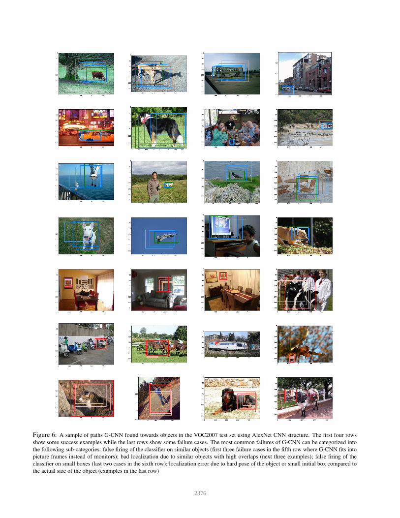
Figure 6: A sample of paths G-CNN found towards objects in the VOC2007 test set using AlexNet CNN structure. The first four rows

show some success examples while the last rows show some failure cases. The most common failures of G-CNN can be categorized into

the following sub-categories: false firing of the classifier on similar objects (first three failure cases in the fifth row where G-CNN fits into

picture frames instead of monitors); bad localization due to similar objects with high overlaps (next three examples); false firing of the

classifier on small boxes (last two cases in the sixth row); localization error due to hard pose of the object or small initial box compared to

the actual size of the object (examples in the last row)

2376

References

[1] H. Azizpour and I. Laptev. Object detection using strongly-

supervised deformable part models. In ECCV, pages 836–

849, 2012. 2

[2] J. Carreira, P. Agrawal, K. Fragkiadaki, and J. Malik. Human

pose estimation with iterative error feedback. arXiv preprint

arXiv:1507.06550, 2015. 1

[3] D. Erhan, C. Szegedy, A. Toshev, and D. Anguelov. Scalable

object detection using deep neural networks. In CVPR, pages

2147–2154, 2014. 2

[4] P. Felzenszwalb, D. McAllester, and D. Ramanan. A dis-

criminatively trained, multiscale, deformable part model. In

CVPR, pages 1–8, 2008. 2

[5] P. F. Felzenszwalb, R. B. Girshick, and D. McAllester. Cas-

cade object detection with deformable part models. In CVPR,

pages 2241–2248, 2010. 2

[6] R. Girshick. Fast r-cnn. In ICCV, pages 1440–1448, 2015.

1, 2, 4, 6, 7

[7] R. Girshick, J. Donahue, T. Darrell, and J. Malik. Rich fea-

ture hierarchies for accurate object detection and semantic

segmentation. In CVPR, pages 580–587, 2014. 2, 3, 5

[8] R. Girshick, J. Donahue, T. Darrell, and J. Malik. Region-

based convolutional networks for accurate object detection

and segmentation. Pattern Analysis and Machine Intelli-

gence, IEEE Transactions on, 38(1):142–158, 2016. 6, 7

[9] K. He, X. Zhang, S. Ren, and J. Sun. Spatial pyramid pooling

in deep convolutional networks for visual recognition. In

ECCV, pages 346–361, 2014. 2, 6

[10] D. Hoiem, Y. Chodpathumwan, and Q. Dai. Diagnosing error

in object detectors. In ECCV, pages 340–353, 2012. 6

[11] A. Krizhevsky, I. Sutskever, and G. E. Hinton. Imagenet

classification with deep convolutional neural networks. In

Advances in neural information processing systems, pages

1097–1105, 2012. 2, 5

[12] C. H. Lampert, M. B. Blaschko, and T. Hofmann. Beyond

sliding windows: Object localization by efficient subwindow

search. In CVPR, pages 1–8, 2008. 1

[13] B. Leibe, A. Leonardis, and B. Schiele. An implicit shape

model for combined object categorization and segmentation.

Springer, 2006. 1

[14] K. Lenc and A. Vedaldi. R-CNN minus R. CoRR,

abs/1506.06981, 2015. 1, 2

[15] S. Maji and J. Malik. Object detection using a max-margin

hough transform. In CVPR, pages 1038–1045, 2009. 1

[16] J. Redmon, S. Divvala, R. Girshick, and A. Farhadi. You

only look once: Unified, real-time object detection. arXiv

preprint arXiv:1506.02640, 2015. 1, 2, 7

[17] S. Ren, K. He, R. Girshick, and J. Sun. Faster r-cnn: Towards

real-time object detection with region proposal networks. In

Advances in Neural Information Processing Systems, pages

91–99, 2015. 2

[18] K. Simonyan and A. Zisserman. Very deep convolutional

networks for large-scale image recognition. arXiv preprint

arXiv:1409.1556, 2014. 2, 5

[19] C. Szegedy, A. Toshev, and D. Erhan. Deep neural networks

for object detection. In Advances in Neural Information Pro-

cessing Systems, pages 2553–2561, 2013. 2

[20] A. Torralba, K. P. Murphy, and W. T. Freeman. Contextual

models for object detection using boosted random fields. In

Advances in neural information processing systems, pages

1401–1408, 2004. 1

[21] J. R. Uijlings, K. E. van de Sande, T. Gevers, and A. W.

Smeulders. Selective search for object recognition. Inter-

national journal of computer vision, 104(2):154–171, 2013.

2

[22] A. Vedaldi, V. Gulshan, M. Varma, and A. Zisserman. Mul-

tiple kernels for object detection. In ICCV, pages 606–613,

2009. 1

[23] D. Yoo, S. Park, J.-Y. Lee, A. S. Paek, and I. So Kweon. At-

tentionnet: Aggregating weak directions for accurate object

detection. In ICCV, pages 2659–2667, 2015. 2

[24] C. L. Zitnick and P. Dollar. Edge boxes: Locating object

proposals from edges. In ECCV, pages 391–405, 2014. 2

2377