g b r :v c large-s p - duke universitypublic.econ.duke.edu/~yildirh/public_good_final.pdf ·...

GETTING THE BALL ROLLING: VOLUNTARY CONTRIBUTIONS

TO A LARGE-SCALE PUBLIC PROJECT

HUSEYIN YILDIRIM

Duke University

Abstract

This paper examines dynamic voluntary contributions to a large-scaleproject. In equilibrium, contributions are influenced by the inter-play of two opposing incentives. While agents prefer to free ride onothers for contributions, they also prefer to encourage others to con-tribute by increasing their own. Main findings of the paper are that(1) agents increase their contributions as the project moves forward;(2) as additional agents join the group, existing agents increase theircontributions in the initial stages of the project while reducing themin the stages close to completion; (3) groups that are formed by morepatient agents and that undertake larger projects tend to be larger;and (4) groups that rely on voluntary contributions tend to be toosmall compared to the social optimum. The empirical evidence oncontributions to open-source software projects provides partial sup-port for these findings.

1. Introduction

The successful completion of many large-scale projects depends on the con-tinuous participation of multiple parties. Although binding contracts wouldbe desirable in these situations, often they are not feasible. There are typi-cally noncontractible uncertainties associated with the projects themselves orwith the participants’ economic and political environments. Moreover, in thecase of international projects, contracts are notoriously hard to enforce dueto the lack of a supranational authority. Binding contracts, however, are not

Huseyin Yildirim, Department of Economics, Duke University, Box 90097, Durham, NC27708 ([email protected]).

I thank an anonymous referee, John Conley (the Editor), Greg Crawford, Elif Ekebas-Yildirim, Wolfgang Koehler, Tracy Lewis, Oksana Loginova, Tom Nechyba, Curt Taylor,and seminar participants at Duke-UNC Micro Theory Workshop, Universities of Wisconsin(Madison) and Florida, 2002 European Meeting of Econometric Society, and 2003 South-ern Economic Association Meetings for helpful comments and suggestions.

Received May 26, 2004; Accepted April 29, 2005.

© 2006 Blackwell Publishing, Inc.Journal of Public Economic Theory, 8 (4), 2006, pp. 503–528.

503

504 Journal of Public Economic Theory

always necessary for the successful completion of large-scale projects involvingmultiple parties.

There have been significant successes in the progress and completionof important projects that rely mostly on voluntary contributions. A notableexample is the open-source software such as Apache, Linux, and GNOME.These large-scale programs are developed by programmers scattered aroundthe world, who voluntarily and freely contribute their valuable time and skills.As of late 2000, the web server Apache was used by more than 59% of ac-tive servers across all domains, and Linux as a server-operating environmentgained 17% market share ( Johnson 2002, Lerner and Tirole 2001, 2002).Other notable examples are the international effort to restore the Earth’sozone layer (Murdoch and Sandler 1997), to clean up rivers crossing inter-national boundaries (Sigman 2002), and to eradicate global terrorism.

What determines the successful completion of a large-scale project thatrelies on voluntary contributions? While a full answer to this question is ob-viously quite complex and context specific, in this paper I construct a fairlygeneral model intended to capture the following salient features of suchprojects: (1) they require voluntary contributions by participants; (2) theyare usually divided into smaller subprojects that are to be completed in a pre-specified order;1 (3) participants possess private information about their keycharacteristics such as current financial and political status, or simply theiroutside opportunities, which fluctuate over time; and (4) the benefits of acompleted project are enjoyed for an extended period of time.

The formal model builds on the discrete public good framework of Palfreyand Rosenthal (1988, 1991). There are N risk-neutral agents who work on ajoint project whose full return is realized only after a sequence of stages hasbeen completed. In each period, the agents simultaneously decide whetheror not to contribute to advancing the project after commonly observing thestate of the project and privately observing their own cost of contributing.The costs of contributing vary across agents and time.

In general, contributions to a joint project suffer from the well-knownfree-rider problem. While agents benefit freely from others’ contributions,they bear the full cost of their own efforts, leading them to rely “too much” onothers. When projects require a sequence of contributions, however, a secondeffect, countervailing the free-riding incentive, emerges. To see this, supposethere is at first a single agent that is initially indifferent about contributingto a public project. Now, suppose this agent is informed that a second agentwould be interested in contributing to the project if it were one step furtheralong or sufficiently “mature.” That is, the second agent’s current valuationof the project is too small to attract his initial contribution. If the free-ridereffect were the only force at play here, then the first agent would continue toremain indifferent about initiating the project. The presence of the second

1For instance, the open source programs are composed of modules of smaller programs.

Getting the Ball Rolling 505

agent, however, can in fact break the first agent’s indifference and cause himto start the project in order to attract future contributions. In a sense, thefirst agent invests in the project in order to free ride on the second agentin the future. Using the terminology of Bolton and Harris (1999),2 I call thelatter effect the “encouragement” effect and examine how it interacts withthe free-riding incentive throughout the relationship.

The organization of the paper and a brief preview of the findings are asfollows. In Section 2, I present the basic model in which agents’ contributionsare perfect substitutes. In the unique symmetric Markov Perfect Equilibrium(MPE), I find that early in the project agents make concessions toward thecompletion of the project through increased efforts. In general, there aretwo opposing effects on an agent’s effort choice arising from increased con-tribution by others: On the one hand, it makes his effort less pivotal therebyfacilitating the free-rider effect. On the other hand, it brings the future re-turns generated by greater future contributions closer thereby facilitatingthe encouragement effect. The latter effect mitigates the former and thus inequilibrium each agent raises his effort level.

In Section 3, I consider group size. An increase in the group size has onedirect and two strategic effects on agents’ contribution decisions. The directeffect comes from the possible “congestion” in the utilization of the com-pleted project such as clean international waters. The strategic effects are theencouragement and the well-known free-riding incentives. When the projectis a noncongestible public good, for example, an open source program, I findthat equilibrium contributions across states are not monotonically affectedby the group size. As one more agent joins the group, the original mem-bers may increase their contributions in some states and reduce it in others.In general, the encouragement effect is stronger in a larger group in theinitial stages of the project—simply because the gain from encouraging oth-ers is greater. However, as the project nears completion, the encouragementeffect loses strength and the free-riding incentive becomes more dominantin a larger group, leading agents to lower their contributions. Despite thisnonmonotonicity, agents strictly benefit from the inclusion of an additionalgroup member. Interestingly, as the group size tends to infinity, the equilib-rium contributions approach to the socially optimal level. This finding runscounter to that of Olson’s (1965) intuition that as the group size increases,the inefficiency in public good provision also increases. Moreover, the em-pirical evidence on programmers’ contributions to open-source software isconsistent with my results as I discuss at length.

When the project is a congestible public good, the congestion effectcounteracts the net positive dynamic effects. In such cases, I consider the

2Although my focus and formal model are considerably different from those in Boltonand Harris (1999), both papers highlight similar dynamic effects, as becomes clear in theanalysis.


optimal group size that balances the congestion and the dynamic effects. Ifind that larger projects require a larger group, but—more interestingly—theoptimal group size increases with agents’ patience. This is because more pa-tient agents are able to better control the free-riding incentive, which allowsthem to include more members to expedite the completion of the project.Nonetheless, in Section 4, I show that groups that rely on voluntary contribu-tions tend to be too small with respect to the “social optimum” where they cancoordinate their actions. Finally, in Section 5, I extend the model to incor-porate complementaries in agents’ efforts and, in Section 6, discuss possibleextensions.

1.1. Related Work

My paper is closely related to two strands of the literature on the private pro-vision of public goods. The first strand investigates the provision of discretepublic goods in static models with incomplete information. See, for example,Menezes et al. (2001) and Palfrey and Rosenthal (1988, 1991).3 My analy-sis however is intended to uncover the incentives in a dynamic setting. Thesecond strand explores the dynamic contribution models with complete in-formation. Most notably, papers by Admati and Perry (1991) and Fershtmanand Nitzan (1991) consider models in which, like mine, contributions ac-cumulate over time to provide a public good. Their main point is that thedynamics exacerbate the free-riding incentive, as agents view their contribu-tions as a substitute not only to current contributions but also to the futureones. In particular, Admati and Perry find that many socially desirable projectsare unlikely to be undertaken. Marx and Matthews (2000) analyze a similarframework but allow for trigger strategies so that if an agent fails to contributehis equilibrium amount, others punish him by delaying theirs. This implicitenforcement alleviates the free-rider incentive and leads to the positive resultsin Marx and Matthews.4

Unlike these papers, my model explores a setting in which agents’ costsof contribution are private information and more importantly, they vary overtime and across agents. I discover that even though agents use more “for-giving” strategies than the ones in Marx and Matthews, the dynamics helpalleviate the free-riding incentives. In particular, while agents free ride on cur-rent contributions, they view future contributions as complementary in mymodel. This means that part of the reason for the negative result in Admati

3Bagnoli and Lipman (1989), and Palfrey and Rosenthal (1984) also study the privateprovision of a discrete public good in a static model but with complete information.4Papers by Bac (1996), McMillan (1979), Palfrey and Rosenthal (1994), and Pecorino(1999) also explore the possibility of cooperation in public good provision in infinitelyrepeated game settings. However, unlike in my model, agents enjoy the full return in eachperiod, and thus the incentives to complete a large-scale public project do not arise.


and Perry (1991), and Fershtman and Nitzan (1991) is the fact that agents’costs of contribution are common knowledge and stay the same over time.

2. The Model

Consider a dynamic extension of Palfrey and Rosenthal (1988, 1991). Thereare N agents who work on a joint project with H subprojects where H is anatural number. The progress of the project is observed by all agents. Let h bethe state variable indicating that (h − 1) subprojects have been completed,and let r(h) denote the corresponding per period return to each agent instate h. The project yields its full return, v(N ) > 0, after all subprojects arecompleted. Namely,

ASSUMPTION 1:

r (h) ={

v(N ), for h > H

0, for h ≤ H,

where v(N ) can be decreasing, constant, or increasing in N , capturing dif-ferent types of projects depending on how participants share the benefits of acompleted project. I call the projects “congestible” if v(N ) is decreasing, and“noncongestible” if v(N ) is constant. I also allow for projects for which v(N )is increasing, perhaps because there are positive externalities in utilizing thefinished project.

Assumption 1 indicates that there are no immediate returns before com-pleting the project. While certain projects might yield intermediate payoffs,as long as the cumulative payoff with the progress of the project weakly in-creases at a weakly increasing rate, the qualitative results in the paper willhold. Furthermore, by making each subproject ex ante identical, I abstractfrom the latter complication to better highlight the dynamics in the model.Zero return, however, is pure normalization.

The interaction among agents is modeled as an infinite horizon Markovgame and the MPE is the solution concept.5 Informally, a MPE induces aperfect equilibrium for all payoff-relevant histories described by the state h.The Markov property requires that agents base their decisions only on theprogress of the project. This property also has intuitive appeal in my setting asI wish to investigate the effects of the project progress on agents’ incentivesto contribute.6 In each period, agents observe the state of the project and

5See, for example, Fudenberg and Tirole (1991, ch. 13) for a review.6In theory, agents can use less “forgiving” strategies for a deviation than the Markov ones.However, as with the international projects, each country will have difficulty punishingothers if there is a defection, either because governments change or because it is hardto prove defection in the presence of incomplete information. Furthermore, focusing onMarkov strategies allows me to determine the minimal level of cooperation agents canachieve.


simultaneously decide whether or not to contribute. Like in Rosenthal andPalfrey’s setting, contribution is a 0–1 decision denoted by the indicator vari-able s.7 In the basic model, I assume as long as one agent contributes, theproject moves to the next state. Otherwise, it stalls one period, and the statedoes not change. The process repeats itself the next period with the up-dated state and with new cost draws for agents. This type of production func-tion assumes agents’ contributions are perfect substitutes. Nonetheless, I willshow that agents’ equilibrium contributions exhibit some intertemporal com-plementarity and discuss a more general production function in Section 5.The cost of contribution or effort comes from a twice continuously differen-tiable cumulative distribution, F (c), which is independently and identicallydistributed over time and across agents.8 The support of distribution is [0, c̄]with c̄ > 0 and F ′(c) = f (c) > 0. Agents discount the future returns and costsby δ ∈ (0, 1).9

Let W i(h, c i) be agent i’s value function when his realized cost is ci andthe project is in state h. Suppose that λ∗

−i (h) is the equilibrium probability thatat least one agent other than i contributes. Agent i, then, solves the followingdynamic program:10

Wi (h, ci ) = maxsi ∈{0,1}

{r (h) + si [−ci + δWi (h + 1)]

+(1 − si )δ[λ∗

−i (h)Wi (h + 1) + (1 − λ∗

−i (h))Wi (h)

]},

(1)

where W i(h) ≡ E c[W i(h, c)] and Ec is the expectation operator with respectto c.11

7In the working paper Yildirim (2005), I also study a continuous contribution extensionand show that the same qualitative results as in the discrete case would arise.8This assumption, aside from being realistic, rules out the strategic learning among agentsin a public good context, which is the topic of Bliss and Nalebuff (1984) and Gradstein(1992), among others. In these papers, agents have private information about their costs ofcontribution, and these costs do not change over time. Thus, as time passes by, agents leakinformation to others often resulting in inefficient delays in contributions. Although thistype of strategic learning is an important element of public good provision, here I abstractfrom this aspect to better focus on the effects of the progress of the project on agents’contribution pattern.9Assuming that agents are ex ante symmetric clearly does not fit the examples in theIntroduction, where it seems more reasonable to consider heterogenous cost distributionsand discount factors. While I leave the generalization for future work, I believe the presentmodel is rich enough to identify the main forces in the generalization.10Note that agents incur the cost at the time they volunteer in this model. This might createex post inefficiency in equilibrium as contributions in excess of one are wasted. However,following we will see that agents take this possibility into account when contributing.11Since time enters only through discounting and the cost distribution is stationary overtime, I drop the time index throughout the analysis. Also, following I show that the valuefunctions exist and are well behaved.


According to (1), agent i decides whether or not to contribute to theproject upon observing the state of the project and his own current cost. Ifhe contributes, that is, si = 1, he bears the full cost of his effort in whichcase the project moves forward with certainty and he receives the discountedexpected continuation value, δW i(h + 1). However, if he decides not to, thatis, si = 0, then he will have to rely on others for contribution. In this instance,he conjectures the expected probability that at least one other agent willcontribute, which in turn determines his discounted future expected contin-uation value, δ[λ∗

−i (h)W i(h + 1) + (1 − λ∗−i (h))W i(h)]. In each decision

though, he receives the return, r(h). Define the following cutpoint:

xi (h) ≡ [1 − λ∗

−i (h)]δ�Wi (h), (2)

where �W i(h) ≡ W i(h + 1) − W i(h).Equation (1) reveals that agent i’s equilibrium strategy simply has the

following cutoff property:12

s∗i (h, c) =

{1, if c ≤ xi (h)

0, otherwise.(3)

We say that as xi(h) increases, so does agent i’s contribution or effort.13,14

According to (2), this effort is monotonic in the likelihood of being the pivotalcontributor and in the discounted net future gains.

As is common in sequential games, I characterize the equilibrium usingbackward induction, and for simplicity, focus on the symmetric one. Start withthe completed project, h > H . Clearly, no further contribution is required inthis state and hence xi(h) = 0 for h > H . This implies that the expected dis-

counted value of the completed project is Wi (H + 1) = v(N )1−δ

, or equivalentlythe average per period return is

W̄i (H + 1) ≡ (1 − δ)Wi (H + 1) = v(N ). (4)

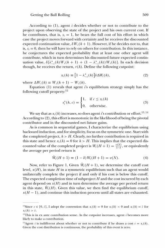
Now, refer to Figure 1. Given W̄i (H + 1), we determine the cutoff costlevel, x(H ), in state H in a symmetric equilibrium such that an agent wouldunilaterally complete the project if and only if his cost is below this cutoff.The expected completion time of subproject H and the cost incurred by eachagent depend on x(H ) and in turn determine the average per period returnin this state, W̄i (H ). Given this value, we then find the equilibrium cutoff,x(H − 1), and continue this induction process until all states are exhausted.

12Since c ∈ [0, c̄], I adopt the convention that xi(h) = 0 for xi(h) < 0 and xi (h) = c̄ forxi (h) > c̄ .13This is in ex ante contribution sense. As the cutpoint increases, agent i becomes morelikely to make a contribution.14Agent i is indifferent about whether or not to contribute if he draws a cost c = xi(h).Given the cost distribution is continuous, the probability of this event is zero.


c

v

)H(xi Cutoff Cost

Value ofthe Project

)(.;B δ

)1(.;B

)1-H(xi00

)H(Wi

)1H(Wi −

Figure 1: Backward induction with substitute contributions

More formally, upon choosing a symmetric cutoff, x, each agent’s ex-pected cost of completing a subproject is given by

B(x; δ) ≡ 1

δ

x[1 − F (x)]N −1

−∫ x

0

[1 − F (c)]dc . (5)

Thus, the equilibrium cutoff, x(H ), has to balance the expected returnand the expected cost, that is, W̄i (H + 1) = B(x(H ); δ). Note that B(x(H ); δ)measures the expected cost in terms of tomorrow’s dollars consistent with thereturn, W̄i (H + 1). Thus, the same cost in today’s dollars, that is, B(x(H ); 1),must be equal to the value of the project in state H . The following lemmarecords the properties of B(•) and shows this induction argument for theremaining states.

LEMMA 1:

(a) For h ≤ H , W̄i (h + 1) = B(x(h); δ), and W̄i (h) = B(x(h); 1), whereW̄i (h) = (1 − δ)Wi (h).

(b) B′(x; δ) > 0 for x ∈ (0, c̄], and B′(0; δ) = 1δ

− 1.


All proofs are contained in the Appendix, which, due to space constraints,is an abbreviated version of the complete Appendix provided in the workingpaper and available on request.

Armed with Lemma 1, the following proposition characterizes theequilibrium:

PROPOSITION 1: There exists a unique symmetric MPE with the following proper-ties. For h ≤ H :

(i) x(h) > 0 for all h.

(ii) x(h) is strictly increasing in h.

(iii) W i(h) is strictly increasing at an increasing rate in h; that is, �W i(h) > 0and �W i(h) > �W i(h − 1).

Part (i) implies that the project of any size is completed despite no im-mediate returns. In equilibrium, agents are willing to take current losses forfuture returns. Two assumptions derive this result: (1) The lower bound ofcost distribution is zero, and (2) contributions are perfect substitutes.15 InSection 5, I consider the case with complementary contributions and comparethe equilibrium behaviors.

The intuition behind part (ii) is more involved. In equilibrium, the cut-point for agent i given in (2) reduces to

xi (h) = [1 − F (x(h))]N −1δ�Wi (h). (6)

Everyone else’s increasing effort has two opposing effects on one’s decisionsummarized on the right hand side of (6): On the one hand, it makes hiseffort less pivotal and thus facilitates the free-rider effect. Formally, as x(h)increases [1 − F (x(h))]N −1 becomes smaller. On the other hand, it bringsfuture returns generated by greater future efforts closer and creates an en-couragement effect given by δ�W i(h). As part (ii) of Proposition 1 indicates,the latter effect mitigates the former, and therefore each agent raises hiseffort as the project moves forward. Put differently, agents view their ownefforts as strategic substitutes for others’ current efforts and as strategic com-plements to the future efforts. This is so in equilibrium even though thereare no complementaries in the production function.16

Since the present model is stationary, one can also determine the av-erage waiting time in each state. Note that the equilibrium probability that

15A strictly positive lower bound on the cost distribution would imply that some large-scaleprojects may not take off. To make the analysis interesting, one would then restrict attentionto the projects that would take off.16The observation in Proposition 1 accords with Bolton and Harris (1999), who considera continuous-time two-armed bandit model of strategic experimentation where agentsprivately choose whether to invest in a safe or risky asset each period. While they alsoidentify free riding and encouragement effects in this social learning environment, myfocus and model are significantly different from theirs. In particular, I consider the issueof private contributions to a large-scale public project and also deal with the optimal groupsize and complementary contributions.


the project will move from state h to h + 1 is given by λ∗(h) ≡ 1 − [1 −F (x(h))]N . Thus, the average waiting time in state h is w(h) = 1

λ∗(h).

Part (ii) of Proposition 1 implies that this waiting time shrinks as the projectmoves forward.

The last part of Proposition 1 reveals that the value agents’ attach to theproject increases at an increasing rate over states.

3. The Effects of Group Size

In general, an increase in the group size has three effects on agents’ contri-bution decisions: one direct effect due to the (possible) change in the payoffafter the project is completed and two strategic effects due to the dynamicsbefore the project is completed. To better understand these effects and dis-tinguish between different types of projects, I first consider noncongestibleprojects for which the direct effect is not present and then consider otherprojects for which it is present.

3.1. Noncongestible Projects

Imagine that participants are contributing toward projects like open-sourcesoftware or restoration of the ozone layer, where an additional user does notdegrade one’s final payoff, that is, v(N ) = v for all N . In this case, an increasein the group size has two opposing strategic effects on agents’ contributions.First, it worsens the well-known free-rider incentive as there are now moreagents to free ride on. Second, it also strengthens the encouragement in-centive, as by increasing one’s own contribution today, an agent can attractgreater future contributions in a larger group. Furthermore, since there aremore future contributions to be made in the initial stages of the project, it isintuitive that the latter incentive will be stronger in those stages while losingits steam with the progress of the project. Thus, it is reasonable to conjecturethat an increase in the group size results in an increase in equilibrium contri-butions in the initial stages of the project and a decrease in the mature stages.I confirm this conjecture in

PROPOSITION 2: Suppose v(N ) = v for all N . For N ≥ 1,

(i) x(H ; N + 1) < x(H ; N ),

(ii) for sufficiently large H, there exists h0 such that for h < h0, x(h; N + 1) >

x(h; N ),

(iii) for h ≤ H , limN →∞x(h; N ) = 0, and limN →∞λ∗(h; N ) = 1.

First two parts of Proposition 2 imply that agents’ contributions are notuniformly affected by an increase in group size. Part (i) reveals that eachagent reduces his equilibrium contribution to the last subproject in a largergroup. Intuitively, since no future contributions are needed in the final stageof the project, the encouragement incentive vanishes and the free-rider effect


0

0.5

1

1.5

2

2.5

3

3.5

1 2 3 4 5 6 7 8 9 10 11 12 13 14 15 16 17 18

State (h)

Cut

off (

x) N=1

N=2

N=3

Figure 2: Nonmonotonicity of contributions

leads to a reduction in contributions. Part (ii) shows that when the project issufficiently large, the encouragement incentive becomes sufficiently strongin the early stages of the project and dominates the free-rider incentive. Togain intuition about how contributions change in the intermediate states withthe group size, I consider a numerical example depicted in Figure 2.

In the example, there are 18 subprojects, that is, H = 18.17 The cost ofeffort is distributed uniformly in [0, 3], and the project yields a value v = 2to each agent upon completion. Also, agents discount future returns by δ =0.9.

Refer to Figure 2. When the group consists of a single agent, obviouslythere are no free-riding or encouragement incentives. In this case, noticethat the agent would finish the project with certainty in the penultimatestate, h = 18, that is, x(18) = c̄ = 3. However, the project virtually does nottake off for the states below h = 6, that is, x(h) ≈ 0 for h ≤ 6. If there is onemore agent in the group, agents encourage each other for the initial 10 statesby choosing higher cutpoints than the single-agent case. Thus, the projectis more likely to take off with a larger group in these states. However, forthe remaining eight states, the free-rider effect becomes stronger resulting inlower effort levels. As the group size grows further to N = 3, the critical statebelow which agents put higher efforts in a larger group goes down. This isbecause with more agents, the project matures faster and the free-rider effectbecomes more dominant starting in an earlier state. The example also showsthat agents’ effort levels stay relatively steady in a larger group.

According to parts (i) and (ii) of Proposition 2 and the example inFigure 2, it is clear that each agent’s contribution in a given state is am-biguous in the group size. Even so, as the group size tends to infinity, each

17Figure 2 shows only states 1 through 18 since we already know that x(h) = 0 for h > 18.


agent expects that someone in the group will draw a cost close to zero andthus chooses a cutpoint close to zero as a result.18 Interestingly, this holds inall states as recorded in part (iii). This does not mean, however, the projectwould never move forward. In contrast, I show in the Appendix that the equi-librium probability that the project moves from h to h + 1, that is, λ∗(h; N ),converges to 1. The increase in the number of agents more than offsets thereduction in the cutpoint.19 In fact, in Section 4, I demonstrate that as N →∞, agents’ welfare approaches to the socially efficient level.

The predictions in Proposition 2 are widely consistent with the empiricalstudies of voluntary contributions by programmers to open-source softwareprojects (see Hertel et al. [2003] for the Linux project; Koch and Schneider[2002] for GNOME project; and Mockus et al. [2000] for the Apache project).These studies report an increase in the average contributions with the numberof programmers, especially in the early stages of the projects, and a declinein the mature stages.20 The fact that more programmers need not reduce thepace of a software project was first argued by Raymond (1999), who made theassertion known as Linus’ Law: “Given enough eyeballs, all bugs are shallow.”This is indeed surprising, because previously it was believed that Brooks’ Law(Brooks 1995) that states “. . . adding people to a late project makes it later . . .

the fact that a woman can have a baby in nine months does not imply that ninewomen can have a baby in one month” holds. Though the two assertions seemconflicting, they are not. In his book, Brooks also suggested an exception tohis law by pointing out “. . . if a project’s tasks are partitionable, you can dividethem further and assign them to . . . people who are added late to the project,”which is also the building block of Raymond’s argument.

Despite the ambiguous effects of group size on agents’ effort levels, agentsdo strictly benefit from an additional group member as I note in

PROPOSITION 3: Suppose v(N ) = v for all N . Then, for h ≤ H , W i(h, N + 1) >

W i(h, N ).

Proposition 3 shows that an increase in the number of agents is a Paretoimprovement in the sense that each agent has a higher welfare in each state.This seems intuitive for the states in which agents increase their effort levels

18Again, the fact that the lower bound of cost distribution is zero is important here.19This result might seem puzzling in light of Mailath and Postlewaite (1990), who, in aone-period mechanism design setting, conclude that as the group size tends to infinity,the probability of supplying the public good converges to zero, even though it should beprovided with probability 1. While both Mailath and Postlewaite’s and my model predictthat as N → ∞, agents would feel less pivotal and reduce their contributions, the differencestems from the fact that Mailath and Postlewaite assume the exogenous cost of providingthe public good increases in group size faster than the free-riding incentive.20Note that the average contribution is F (x(h)) in my model.


as this improves the pace of the project resulting in a higher value.21 However,when the project matures, an additional agent exacerbates the free-riderincentive and might even slow down the progress of the project. Even so,the cost saving associated with one additional agent more than offsets thisreduced pace. Thus, Proposition 3 implies that the optimal group size fornoncongestible projects is infinity. Once again this is consistent with the factthat open source projects accept contributions from programmers all overthe world rather than restricting the group to just a few.

In light of Proposition 3, I should also note that the qualitative resultspertaining to congestible projects trivially hold when there are positive ex-ternalities in the utilization of the project, that is, v(N ) increases in N . Inparticular, both the direct and the net dynamic effects are positive. However,this is not the case in what follows with congestible projects.

3.2. Congestible Projects and the Optimal Group Size

When the completed project is a congestible public good, the direct conges-tion effect of the group size counteracts the net positive effect identified inProposition 3. How the group balances the two effects depends on its abilityto restrict entry into the group. It is thus important to ask what the optimalgroup size is. To put the analysis into perspective, I assume that the congestionis sufficiently severe for large groups.

ASSUMPTION 2:

limN →∞ v(N ) = 0.

From Assumption 2, it easily follows that when the entry into the groupcannot be restricted, the payoff will be driven down to zero after the projectis completed. In such situations, the project will not be undertaken. Thisis the extreme case of congestion. However, suppose that the access can berestricted or simply that the project is an excludable public good. In thesecases, I will assume that the optimal group size is the one that maximizes eachmember’s expected net present value of the project, W̄i (1, N | δ, H ), beforethe project starts.22 Let N ∗(H , δ) be the optimal group size for a project withH subprojects and an individual discount factor of δ. More formally, sincefrom Lemma 1, W̄i (1, N | δ, H ) = B(x∗(N , δ); 1 | N , H ), we have

21This is clearly seen from Lemma 1 where B(x; 1) is strictly increasing in x.22While I am not explicitly modeling how the group actually forms, one can imagine thatone agent offers memberships to other ex ante identical agents, each of whom then eitheraccepts or declines the offer. There are however no side payments. In this case, it is clearthat the number of offers the first agent makes will maximize his expected discounted valueof the project. Notice also that N ∗ maximizes the ex ante average per period payoff ratherthan just the discounted payoff. This allows me to isolate the strategic effect of discounting.


N ∗(H, δ) = arg maxN

B(x∗(N , δ); 1 | N , H ). (7)

The result in Proposition 3 for noncongestible projects along with As-sumption 2 imply that N ∗(H , δ) exists and finite. In what follows, I assume itis also unique. The following result records how the group size changes withthe project size and the agents’ discounting.

PROPOSITION 4: Suppose that the project is an excludable public good and As-sumption 2 holds. Then, the optimal group size (weakly) increases with the project sizeand with agents’ patience level.

To see the intuition behind the link between the group size and projectscale, note that having the same number of participants that is optimalfor a smaller project cannot be excessive for a larger project. Given thesame group size, the return from a completed project remains the sameacross different size projects. But this means agents would prefer more en-try into the group in order to finish a larger project in a shorter time(Proposition 3).

The intuition behind the second part of the proposition is more involved.For a fixed group size, an increase in the discount factor has three effects onagent i’s contribution: First, since he now cares more about the future, heis willing to take larger current losses and thus increases his cutpoint in (6).Second, given that others contribute more in response to a higher δ, agenti’s contribution becomes less pivotal, that is, [1 − F (x(h; δ))]N −1 is smaller,and thus he tends to free ride and decrease his contribution. Third, others’increasing contributions brings the future returns generated by future con-tributions closer and thus encourages agent i. Overall, agent i’s contributionincreases with δ. This implies that more patient agents are able to control thefree-riding incentive more effectively, which in turn allows them to expandthe group and expedite the completion of the project.23 Next, I investigatewhether or not the group tends to be too large or too small with respect tothe social optimum.

23The fact that more patient agents can control free-riding incentives more effectively istrue despite there being no reputational concerns in my setting, which is in contrast toseveral other dynamic models of public good provision, for example, Bac (1996), Marxand Matthews (2000), McMillan (1979), and Pecorino (1999), where agents adopt triggerstrategies. In such settings, as the discount factor becomes larger and agents become morepatient, the punishment becomes more severe for any deviation, which helps sustain thecooperative outcome. Here, I focus on the Markov property that excludes such triggerstrategies. Nonetheless, the relationship grows to be more cooperative in response to ahigher discount factor.


4. Benchmark: Social Optimum

There are two sources of inefficiencies in the noncooperative contributiongame I have analyzed: (1) Agents simultaneously choose their cutoff points,and (2) agents have incomplete information about others’ costs of contri-bution. The first best would occur if neither of these problems existed. Theoptimal strategy in this case would be to assign the project to the lowest costagent in each state unless this cost is too high. However, given the informa-tional constraints, this solution is infeasible in the present setting, which relieson voluntary contributions. Therefore, the second-best situation where thesocial planner coordinates agents’ cutpoints before the costs of contributionare realized seems more appropriate as a benchmark.

Suppose a social planner maximizes the total welfare, or equivalently theaverage welfare per agent in the group by choosing a cutpoint, x∗∗

i (h), foragent i.24 Let W ∗∗(h) be the optimal average payoff per agent in state h. Itis clear that once the project is completed, the social planner will choosex∗∗

i (h) = 0 for h > H , and thus have no agent contribute. This implies the

boundary condition as in (4): For h > H, W ∗∗(h) = v(N )1 − δ

. For h ≤ H , however,W ∗∗(h) satisfies the following dynamic program:

W ∗∗(h) = 1

1 − δmax{xi (h)}

{− 1

N

N∑i=1

∫ xi (h)

0

c dF (c)

+[

1 −N∏

i=1

(1 − F (xi (h)))

]δ�W ∗∗(h)

}, (8)

where the first term inside maximization is the average cost, and the secondterm is the probability that the project will move to the next state times theexpected increase in the value of the project. The first-order condition forxi(h) implies that

x∗∗i (h) = [

1 − λ∗∗−i (h)

]N δ�W ∗∗(h), (9)

where again λ∗∗−i(h) represents the optimal probability that at least one agent

other than i will contribute.25

Comparing (9) and (2), we see that when determining the cutoff foragent i, the social planner takes the effect of i’s contribution on the totalwelfare rather than just on i’s own welfare. As before, I will assume that thesocial planner optimally assigns symmetric cutoff points to all agents, that is,x∗∗

i (h) = x∗∗(h). Now define the following function analog of (5):

24Alternatively, suppose agents are able to write a one-period contract on their cutoffs beforecosts of contribution are realized.25It is easy to verify that the maximized function is strictly quasiconcave.


B∗∗(x) = xδN [1 − F (x)]N −1

−∫ x

0

[1 − F (c)]dc +(

1 − 1

N

)x[1 − F (x)].

(10)

A variant of Lemma 1 records how the social planner uses backward inductionto find the optimal cutoff points.

LEMMA 2:

(a) For h ≤ H, W̄ ∗∗(h + 1) = B∗∗(x∗∗(h); δ), and W̄ ∗∗(h) = B∗∗(x∗∗(h); 1)where W̄ ∗∗(h) = (1 − δ)W ∗∗(h).

(b) B∗∗′(x; δ) > 0 for x ∈ (0, c̄], and B∗∗′(0; δ) = 1N ( 1

δ− 1).

Given that the qualitative properties of B∗∗(x; δ) coincides with that ofB(x; δ), the existence of a unique social optimum easily follows by applyingthe proof of Proposition 1. Here we are interested in knowing whether the co-ordination of efforts strictly benefit agents in all states, and more importantlywhether the project progresses at the socially optimal rate. The followingproposition answers these questions.

PROPOSITION 5: For N > 1, and h ≤ H :

(i) W i(h) < W ∗∗(h).

(ii) x(h) < x∗∗(h).

(iii) limδ→1x(h) = x1 < limδ→1x∗∗(h) = x∗∗1 .

According to part (i) of Proposition 5, agents strictly benefit from coor-dinating their efforts. This is because the equilibrium cutpoints are in thesocial planner’s choice set. Part (ii) implies that agents contribute too infre-quently to the project and thus the project progresses too slowly from thesocial standpoint. This means the positive encouragement effect cannot fullymitigate the negative free-rider effect in our model. This inefficiency remainseven when the discounting is negligible as recorded in part (iii).

Next, I investigate the degree of inefficiencies caused by an increase inthe group size when the project is a noncongestible public good and comparethe optimal group size with the benchmark when it is a congestible publicgood. Let N ∗∗(H , δ) be the socially optimal group size for a congestibleproject.

PROPOSITION 6:

(i) If the project is a noncongestible public good, that is, v(N ) = v, thenlimN →∞Wi (h) = limN →∞W ∗∗(h) = δH+1−h

1−δv.

(ii) If the project is congestible and Assumption 2 holds, then N ∗(H ; δ) ≤N ∗∗(H , δ).


The first part of Proposition 6 reveals that as the group size grows withoutbound for a noncongestible project, the inefficiencies disappear and agents’expected payoffs converge to the socially optimal one. Together with part (iii)of Proposition 2, this result goes against our intuition from Olson (1965), whoasserts “. . . the larger the group, the farther it will fall short of providing anoptimal amount of collective good”(p. 35). The main difference comes fromthe fact that the technology in my model is that of a “best shot” one, whichrequires only one contribution in each stage. Thus, in both the incompleteinformation and the second-best cases, as the group size becomes sufficientlylarge, the contribution is made by the lowest cost agent and the expectedprobability of having such an agent converges to one in the limit.

The second part implies that groups that rely on voluntary contributionstend to be too small with respect to the social optimum. The intuition is clear:In the social optimum, agents are able to coordinate their strategies so thatthey can control the free-riding incentive more easily. This allows the groupto include more members in order to finish the project in a shorter time.Conversely, when the coordination of strategies is not feasible, the groupcontrols the free-riding incentive by being small.

5. Complementary Contributions

Until now, I have assumed that agents’ contributions are perfect substitutesin that in a given period if at least one of them contributes, the project movesforward. Although this is the case for open-source software, or projects thatrequire only the financial contributions, for example, other projects mightrequire certain degree of complementarity in agents’ efforts. To capture thispossibility, suppose that at least m ∈ {1, . . . , N } agents need to contributein a given period for the project to move forward. We say that a higher mcorresponds to a higher degree of complementarity in production with m =1 and m = N being the two polar cases representing perfect substitutes andperfect complements, respectively. An increase in the degree of complemen-tarity has two opposing effects on the group interaction: (1) It reduces thefree-rider problem by making agents’ contributions less substitutable, and (2)it exacerbates the coordination problem by requiring others’ contributionsto make one’s own worthwhile.

Let λ∗−i (m, h) be the equilibrium probability that at least m agents other

than i contribute in state h. Like in perfect substitute case, agent i solves thefollowing dynamic program to decide whether or not to contribute in stateh:

Wi (h, ci ) = maxsi ∈{0,1}{

r (h) + si[ −ci + δ

[λ∗

−i (m − 1, h)Wi (h + 1) + (1 − λ∗

−i (m − 1, h))Wi (h)

]]+ (1 − si )δ

[λ∗

−i (m, h)Wi (h + 1) + (1 − λ∗

−i (m, h))Wi (h)

}. (11)


It is clear from (11) that agent i adopts a similar cutoff strategy to (2)with the following cutpoint:

xi (h) = [λ∗

−i (m − 1, h) − λ∗−i (m, h)

]δ�Wi (h). (12)

Note that the expression, λ∗−i(m − 1, h) − λ∗

−i(m, h), is the probabil-ity that agent i’s contribution is pivotal. Thus, the intuition behind (12) isthe same as in the substitute case. In equilibrium, agents optimally choosezero contributions once the project is completed, that is, xi(h) = 0 forh > H . For the intermediate states, the zero contribution continues to be anequilibrium representing a complete coordination failure whenever there iscomplementarity, m ≥ 2. However, there might be other equilibria in whichall agents do contribute and which are clearly Pareto improving over thezero-contribution equilibrium. I will assume that agents coordinate on themost favorable equilibrium in each state.26 Below, I demonstrate that despiteagents’ best efforts to overcome coordination problem, some projects maynever start. Since the coordination problem gets worse in a larger group,I focus on noncongestible projects to abstract from further negative effectdue to congestion. But I should note that the following qualitative results arestrengthened by congestion. Furthermore, to simplify the formal exposition,I only consider the perfect complement case where the project requires fullparticipation of agents in each stage and assume F (c) = ( c

c̄ )α, α > 0. How-

ever, the essential intuition for the general case remains the same.27 To de-termine the symmetric equilibrium, define the following function analog of(5):

BC (x; δ) = 1 − δ

δ

xF (x)N −1

+∫ x

0

F (c)dc .

LEMMA 3: For h ≤ H : W̄i (h + 1) = BC (x(h); δ), and W̄i (h) = BC (x(h); 1),where W̄i (h) = (1 − δ)Wi (h).

The following proposition characterizes the equilibrium.

PROPOSITION 7: There exists a unique symmetric MPE with the followingproperties:

(i) If 1 − α(N − 1) ≤ 0, then sufficiently large projects or projects witha sufficiently low final value, v < vmin, where vmin ≡ BC (xmin; δ) and

26Palfrey and Rosenthal (1988, 1991) also consider complementary contributions case andnote the multiplicity of equilibria. They use the notion of an equilibrium being globallyexpectationally stable, which can be used in my setting to eliminate the zero-contributionequilibrium whenever another equilibrium exists.27In particular, for a given degree of complementarity, the project may not start, dependingcrucially on the cost distribution and group size.


xmin = { 1 − δδ

[α(N − 1) − 1]} 1αN c̄ never start and all other projects start with

positive probability.

(ii) If 1 − α(N − 1) > 0, then all projects start with positive probability.

(iii) The projects that start have the following properties: For h ≤ H : x(h) is strictlyincreasing in h, and W i(h) is strictly increasing at an increasing rate in h .

Part (i) of Proposition 7 implies that when agents’ contributions are com-plementary, large-scale projects may not start at all. This is unlike the substi-tute case where all projects take off (Part (i) of Proposition 1). The fact thatagent i’s contribution is valuable only when other agents contribute createsa coordination problem and raises his “effective” cost of contribution. Thiscost may prove to be too high compared to the expected value of the project.Like Figure 1, Figure 3 demonstrates the backward induction described inLemma 3 when there are complementaries in agents’ inputs. Note, however,that unlike in Figure 1, there are no positive x(h)’s for projects longer thanthree stages. This means projects larger than three stages fail to take off.

c

v

)H(xi Cutoff Cost

Value ofthe Project

)(.;BC δ

)1(.;BC

0

)H(Wi

)1H(Wi −

)1-H(xi)2-H(xi

minv

Figure 3: Backward induction with complementary contributions


The conditions in (i) and (ii) provide intuition regarding the roles ofthe discount factor, group size, and the cost distribution in coordination fail-ure. As δ increases, it is more likely that the project of any size will start.In fact, as δ → 1, all projects start. The coordination failure worsens asgroup size increases and high costs become more likely. For a given distri-bution, the maximum group size that would satisfy the condition in part (ii)is N̄ = 1

α. For instance, when α = 1

2, a two-agent group will start any project.

If the group size exceeds 2, some projects may not take off. This suggeststhat projects with complementary efforts might require outside help for anumber of stages to insure that the rest will be finished through voluntarycontributions.

This finding has similar flavor to that of Andreoni (1998), who consid-ers the role of fundraising activities in inducing subsequent voluntary con-tributions. Within a one-shot contribution game with complete information,Andreoni assumes that contributions need to exceed some exogenous thresh-old level to yield any return. He notes that when contributions are perfectsubstitutes, the zero-contribution equilibrium exists if this threshold is toohigh. Therefore, an outside help, for example, an initial pledge or a govern-ment grant is needed to break this rather inefficient equilibrium and generatefuture voluntary contributions. The nonconvexity in my model is due to thecomplementaries in agents’ contributions creating a complete coordinationfailure when agents’ values of the project are very low.

Part (iii) indicates that once the project starts, the relationship amongagents grows like in the substitute case.

6. Concluding Remarks

I have considered in some detail how participants voluntarily contribute to alarge-scale project that consists of a sequence of subprojects. While the analy-sis has produced novel insights, it has also maintained restrictive assumptions.For one, the project is assumed to move only one step at a time regardlessof the number of contributions. A more general approach would allow fora “smoother” production function and facilitate a performance comparisonacross projects with different technologies. Second, a number of richer strate-gies is ruled out by the MPE concept. For instance, if the project is an exclud-able public good, agents may adopt a time-dependent strategy that excludespartners who failed to contribute for a period of time. It would be interestingto see what the equilibrium “grace period” would be and how it would com-pare to the socially optimal one. Third, the analysis takes the division of theproject as exogenous. An important extension would study the optimal divi-sion of the project and see how the division would be affected by the numberof participants and the cost distribution. Finally, agents may be heterogenousin their key variables such as their cost distributions and discount factors. Forinstance, one country’s financial fluctuation reflected by its cost distributionor political stability summarized by its discount factor can be different from


another. An extension that allows for such heterogeneity can shed light onits role on cooperation.

Appendix

Proof of Lemma 1: Using (1) and (3) in the text, take the following expecta-tion:

Wi (h) = Ec [Wi (h, c)]

=∫ xi (h)

0

[−c + δWi (h + 1)]dF (c)

+∫ c̄

xi (h)

δ[λ∗

−i (h)Wi (h + 1) + (1 − λ∗

−i (h))Wi (h)

]dF (c).

(A1)

Integrating the first integral by parts yields

Wi (h) = −xi (h)F (xi (h)) + δWi (h + 1)F (xi (h)) +∫ xi (h)

0

F (c)dc

+ δ[λ∗

−i (h)Wi (h + 1) + (1 − λ∗

−i (h))Wi (h)

][1 − F (xi (h))].

(A2)

Now, recall from (2) that

xi (h) = [1 − λ∗

−i (h)]δ�Wi (h). (A3)

Using (A3) successively, (A2) reduces to

Wi (h) = δWi (h + 1) −∫ xi (h)

0

[1 − F (c)]dc . (A4)

Moreover, (A3) implies that

Wi (h) = Wi (h + 1) − xi (h)

δ[1 − λ∗

−i (h)] . (A5)

Together with (A5), (A4) reveals that

W̄i (h + 1) = (1 − δ)Wi (h + 1)

= B(x(h); δ), (A6)

where I make use of the symmetric equilibrium assumption so thatxi(h) = x(h) for all i in equilibrium and

B(x; δ) ≡ 1

δ

x[1 − F (x)]N −1

−∫ x

0

[1 − F (c)]dc, (A7)

as defined in (5) in the text.


Substituting for W i(h + 1) from (A5) into (A4) also implies that

W̄i (h) = (1 − δ)Wi (h)

= B(x(h); 1),(A8)

completing the proof of part (a) of Lemma 1.Now differentiate B(x; δ) with respect to x to find

B′(x; δ) = 1

δ

[1

(1 − F (x))N −1+ (N − 1)xf (x)

(1 − F (x))N

]− (1 − F (x)). (A9)

Since for x ∈ [0, c̄], 1(1 − F (x))N −1 − (1 − F (x)) ≥ 0, we have B′(x; δ) > 0.

Also, (A9) implies that B′(0; δ) = 1δ

− 1. �Proof of Proposition 1: I use backward induction. Note first that since the

payoff does not change for states h > H , we have �W i(h) = 0. Then,(A3) implies that the unique equilibrium is x(h) = 0 for h >H , yieldingthe boundary condition in (4): For h > H ,

W̄i (h) = v(N ). (A10)

Consider h = H . From (A6), x(H ) solves the following equation:

v(N ) = B(x(H ); δ). (A11)

For N = 1, if v(N ) ≥ B(c̄ ; δ), then x(H ) = c̄ . However, if v(N ) <

B(c̄ ; δ), then since v(N ) > 0 and B(0; δ) = 0, the Intermediate ValueTheorem implies there exists x(H ) ∈ (0, c̄) that solves (A11). For N ≥ 2,since v(N ) > 0, B(0; δ) = 0, and B(c̄ ; δ) = ∞, there exists x(H ) ∈ (0, c̄)that solves (A11). Moreover, x(H ) is unique due to B′(x; δ) > 0. Also from(A8),

W̄i (H ) = B(x(H ); 1)< B(x(H ); δ) ≤ v(N ). (A12)

Thus, we have W̄i (H ) < W̄i (H + 1).Now suppose for some j ≥ 0, there exists a unique x(H − j) ∈ (0, c̄)

and W̄i (H − j) < W̄i (H − j + 1). Again, from (A6), x(H − j − 1) solves

W̄i (H − j) = B(x(H − j − 1); δ). (A13)

Since W̄i (H − j) > 0, using a similar argument above, there exists aunique x(H − j − 1) ∈ (0, c̄) that solves (A13). Furthermore,

W̄i (H − j − 1) = B(x(H − j − 1); 1)

< B(x(H − j − 1); δ) = W̄i (H − j).(A14)

Since x(H − j) uniquely solves W̄i (H − j + 1) = B(x(H − j); δ) andx(H − j − 1) solves (A13), given that W̄i (H − j) < W̄i (H − j + 1) bythe induction hypothesis and B′(x; δ) > 0, we have


x(H − j − 1) < x(H − j). (A15)

Hence, there exists a unique symmetric MPE where for h ≤ H , x(h) isstrictly positive and increasing in h.

To prove the last part of Proposition 1, note that in equilibrium (A3)can be written as

x(h) = [1 − F (x(h)]N −1δ�Wi (h). (A16)

Since x(h) is strictly increasing for h ≤ H , we must have

�Wi (h − 1) < �Wi (h). (A17)

�LEMMA A1: For sufficiently large H, there exists h0 such that for h < h0, x(h) isarbitrarily close to 0.

Proof of A1: Recall from Proposition 1 that the sequence {x(h)}h=Hh=1 is strictly

increasing or by reordering, the sequence {x(h)}h=1h=H is strictly decreas-

ing. Since the latter sequence is bounded below by 0, it converges to somexl ≥ 0; and so does its subsequence {x(h + 1)}h=1

h=H . Using Lemma 1, thisimplies that there exists h0 such that for h < h0, limH→∞B(x(h + 1); 1) =limH→∞B(x(h); δ). Since B(•) is continuous in x, this further impliesthat B(xl ; 1) = B(xl ; δ), whose unique solution is xl = 0. �

Proofs of Proposition 2 and 3: Suppose v(N ) = v for all N . I first show byinduction that for any N ≥ 1, W i(h, N + 1) >W i(h, N ) for any h ≤ H .

Suppose in equilibrium that W i(H , N + 1) ≤ W i(H , N ). SinceWi (H + 1, N + 1) = Wi (H + 1, N ) = v

1 − δ, we have �W i(H , N + 1) ≥

�W i(H , N ). Then, (A16) implies x(H , N + 1) ≥ x(H , N ). Since B(x; 1)is strictly increasing in x and N , (A8) reveals that W i(H , N + 1) > W i(H ,N ), which is a contradiction. Hence, W i(H , N + 1) >W i(H , N ).

To complete the induction argument, suppose W i(h, N + 1) >W i(h,N ) for some h ≤ H . Suppose, on the contrary, that W i(h − 1, N + 1) ≤W i(h − 1, N ). Since W i(h, N ) is strictly increasing in h for any given N ,we have

Wi (h − 1, N + 1) ≤ Wi (h − 1, N ) < Wi (h, N ) < Wi (h, N + 1). (A18)

Equation (A18) implies that �W i(h − 1, N + 1) > �W i(h − 1, N ). Again,(A16) implies that x(h − 1, N + 1) ≥ x(h − 1, N ), which, in turn, impliesW i(h − 1, N + 1) >W i(h − 1, N ), yielding a contradiction. Hence,W i(h − 1, N + 1) > W i(h − 1, N ). This completes the proof ofProposition 3.

Now I prove part (i) of Proposition 2. Suppose, by wayof contradiction, that x(H , N + 1) ≥ x(H , N ). From above,we know that W i(H , N + 1) > W i(H , N ). Again, given thatWi (H + 1, N + 1) = Wi (H + 1, N ) = v

1 − δ, we have �W i(H , N + 1) <

�W i(H , N ). From here, (A16) implies x(H , N + 1) < x(H , N ), a con-tradiction. Hence, x(H , N + 1) < x(H , N ).


To prove the last part of Proposition 2, note the following first-orderTaylor expansion for x sufficiently close to 0:

B(x; δ) ≈ B(0; δ) + B′(0; δ)x

≈(

1

δ− 1

)x. (A19)

Since, from Lemma A1, we know that for a sufficiently large H , thereexists h0 such that for h < h0, x(h, N ) is arbitrarily close to 0, (A6) and(A19) imply that

W̄i (h, N + 1) ≈(

1

δ− 1

)x(h, N + 1)

W̄i (h, N ) ≈(

1

δ− 1

)x(h, N ).

Furthermore, since W̄i (h, N + 1) > W̄i (h, N ) from Proposition 3, wemust have x(h, N + 1) > x(h, N ).

To prove part (iii), first recall from part (i) that {x(H ; N )}N =∞N =1 is

a strictly decreasing sequence. Since it is bounded below by 0, it mustconverge to some α ≥ 0. Suppose α > 0. For any N , x(H ; N ) uniquelysolves the equation B(x(H ; N )) = v. Given limN →∞x(H ; N ) = α > 0, wehave limN →∞B(x(H ; N )) = ∞ �= v. Hence, α = 0.

Now take any h < H . Since x(h; N ) is increasing in h, we have

0 ≤ x(h; N ) ≤ x(H ; N ).

This implies

0 ≤ limN →∞

x(h; N ) ≤ limN →∞

x(H ; N ) = 0.

Thus, limN →∞x(h; N ) = 0.To complete the proof, suppose limN →∞[1 − F (x(h; N )]N > 0. But

given that limN →∞x(h; N ) = 0, we have limN →∞B(x(h; N )) = 0 �= v > 0.Thus, it must be that limN →∞[1 − F (x(h; N )]N = 0. �

References

ADMATI, A. R., and M. PERRY (1991) Joint projects without commitment, Review ofEconomic Studies 58, 259–276.

ANDREONI, J. (1998) Toward a theory of charitable fund-raising, Journal of PoliticalEconomy 106, 1186–1213.

BAC, M. (1996) Incomplete information and incentives to free ride, Social Choice andWelfare 13, 419–432.


BAGNOLI, M., and B. L. LIPMAN (1989) Provision of public goods: Fully implement-

ing the core through private contributions, Review of Economic Studies 56, 583–602.

BLISS, C., and B. NALEBUFF (1984) Dragon-slaying and ballroom dancing: The

private supply of a public good, Journal of Public Economics 25, 1–12.

BOLTON, P., and C. HARRIS (1999) Strategic experimentation, Econometrica 67, 349–

374.

BROOKS, F. P. (1995) The Mythical Man-Month: Essays on Software Engineering . Reading,

MA: Addison-Wesley.

FERSHTMAN, C., and S. NITZAN (1991) Dynamic voluntary provision of public

goods, European Economic Review 35, 1057–1067.

FUDENBERG, D., and J. TIROLE (1991) Game Theory. Cambridge, MA: MIT Press.

GRADSTEIN, M. (1992) Time dynamics and incomplete information in the private

provision of public goods, Journal of Political Economy 100, 1236–1244.

HERTEL, G., S. NIEDNER, and S. HERMANN (2003) Motivation of software devel-

opers in open source projects: An internet-based survey of contributors to the

Linux Kernel, Research Policy 32, 1159–1177.

JOHNSON, J. (2002) Open source software: Private provision of a public good, Journalof Economics and Management Strategy 11, 637–662.

KOCH, S., and G. SCHNEIDER (2002) Effort, cooperation and coordination in an

open source project: GNOME, Information Systems Journal 12, 27–42.

LERNER, J., and J. TIROLE (2001) The open source movement: Key research ques-

tions, European Economic Review 45, 819–826.

LERNER, J., and J. TIROLE (2002) Some simple economics of open source, Journalof Industrial Economics 50, 197–234.

MAILATH, G., and A. POSTLEWAITE (1990) Asymmetric information bargaining

problems with many agents, Review of Economic Studies 57, 351–367.

MARX, L., and S. MATTHEWS (2000) Dynamic voluntary contribution to a public

project, Review of Economic Studies 67, 327–358.

McMILLAN, J. (1979) Individual incentives in the supply of public inputs, Journal ofPublic Economics 12, 87–98.

MENEZES, F. M., P. K. MONTEIRO, and A. TEMIMI (2001) Private provision of dis-

crete public goods with incomplete information, Journal of Mathematical Economics35, 493–514.

MOCKUS, A., R. FIELDING, and J. HERBSLEB (2000) A case study of open source

software development: The apache server, in Proceedings of the 22nd Interna-

tional Conference on Software Engineering, Limerick, Ireland, pp. 263–272.

MURDOCH, J., and T. SANDLER (1997) The voluntary provision of a pure public

good: The case of reduced CFC emissions and the montreal protocol, Journal ofPublic Economics 63, 331–349.

OLSON, M. (1965) The Logic of Collective Action. Cambridge, MA: Harvard University

Press.


PALFREY, T., and H. ROSENTHAL (1984) Participation and the provision of discrete

public goods: A strategic analysis, Journal of Public Economics 24, 171–193.

PALFREY, T., and H. ROSENTHAL (1988) Private incentives in social dilemmas: The

effects of incomplete information and altruism, Journal of Public Economics 35,

309–332.

PALFREY, T., and H. ROSENTHAL (1991) Testing game theoretical models of free-

riding: New evidence on probability bias and learning, in Laboratory Researchin Political Economy, T. Palfrey, ed. Ann Arbor: University of Michigan Press,

pp. 239–268.

PALFREY, T., and H. ROSENTHAL (1994) Repeated play, cooperation and coordina-

tion: An experimental study, Review of Economic Studies 61, 545–565.

PECORINO, P. (1999) The effect of group size on public good provision in a repeated

game setting, Journal of Public Economics 72, 121–134.

RAYMOND, E. S. (1999) The Cathedral and Bazaar . Sebastopol, CA: O’Reilly Open

Books.

SIGMAN, H. (2002) International spillovers and water quality in rivers: Do countries

free ride? American Economic Review 92, 1152–1159.

YILDIRIM, H. (2005) Getting the ball rolling: Voluntary contributions to a large-scale

public project, Duke University, Department of Economics, Working Paper 02-04.

g b r :v c large-s p - duke universitypublic.econ.duke.edu/~yildirh/public_good_final.pdf ·...

Documents