fuzzy logic design tools - imse-cnm.csic.es · fuzzy logic design tools v. 3.5, march 2018 . toc 2...

FUZZY LOGIC

DESIGN TOOLS

V. 3.5, March 2018

TOC

2

[email protected]

©IMSE-CNM 2018

Copyright (c) 2018, Instituto de Microelectrónica de Sevilla (IMSE-CNM)

All rights reserved.

Redistribution and use in source and binary forms, with or without modification, are permitted provided that the following conditions are met:

Redistributions of source code must retain the above copyright notice, this

list of conditions and the following disclaimer. Redistributions in binary form must reproduce the above copyright notice,

this list of conditions and the following disclaimer in the documentation

and/or other materials provided with the distribution. Neither the name of the IMSE-CNM nor the names of its contributors may be

used to endorse or promote products derived from this software without specific prior written permission.

THIS SOFTWARE IS PROVIDED BY THE COPYRIGHT HOLDERS AND CONTRIBUTORS

"AS IS" AND ANY EXPRESS OR IMPLIED WARRANTIES, INCLUDING, BUT NOT

LIMITED TO, THE IMPLIED WARRANTIES OF MERCHANTABILITY AND FITNESS FOR

A PARTICULAR PURPOSE ARE DISCLAIMED. IN NO EVENT SHALL THE COPYRIGHT

HOLDERS OR CONTRIBUTORS BE LIABLE FOR ANY DIRECT, INDIRECT,

INCIDENTAL, SPECIAL, EXEMPLARY, OR CONSEQUENTIAL DAMAGES (INCLUDING,

BUT NOT LIMITED TO, PROCUREMENT OF SUBSTITUTE GOODS OR SERVICES;

LOSS OF USE, DATA, OR PROFITS; OR BUSINESS INTERRUPTION) HOWEVER

CAUSED AND ON ANY THEORY OF LIABILITY, WHETHER IN CONTRACT, STRICT

LIABILITY, OR TORT (INCLUDING NEGLIGENCE OR OTHERWISE) ARISING IN ANY

WAY OUT OF THE USE OF THIS SOFTWARE, EVEN IF ADVISED OF THE POSSIBILITY OF SUCH DAMAGE.

mailto:[email protected]

TOC

3

Tabla de Contenidos

Release notes for version 3.5 …………………………………………………………………………… 4

Installation of Xfuzzy 3.5 ………………………………………………………………………………….. 7

An Overview of Xfuzzy 3 …………………………………………………………………………………… 8

XFL3: The Xfuzzy 3 specification language ………………………………………………………… 9

o Operator sets ………………………………………………………………………………………. 10

o Types of linguistic variables …………………………………………………………………. 11

o Rule bases …………………………………………………………………………………………… 12

o Crisp blocks ……………………………………………………………………....................... 14

o System global behavior ……………………………………………………………………….. 14

o Function packages ……………………………………………………………………………… 15

Binary function definition

Unary function definition

Crisp function definition

Membership function definition

Membership function family definition

Defuzzification method definition

The standard package xfl

The Xfuzzy 3 development environment ………………………………………………………….. 35

o Description stage ………………………………………………………………………………… 36

System edition (xfedit)

Package edition (xfpkg)

o Verification stage ………………………………………………………………………………... 50

Graphical representation (xfplot)

Inference monitor (xfmt)

System simulation (xfsim)

o Tuning stage ……………………………………………………………………………………….. 60

Knowledge acquisition (xfdm)

Time series prediction (xftsp)

Supervised learning (xfsl)

Simplification (xfsp)

o Synthesis stage ……………………………………………………………………………………. 78

C code generator (xfc)

C++ code generator (xfcpp)

Java code generator (xfj)

VHDL code generator (xfvhdl)

SysGen models generator (xfsg)

TOC

4

Release Notes for version 3.5

Changes in version 3.5 with respect to 3.3

New functionality:

1. The graphical user interface of Xfuzzy now shows the specifications by

means of drop-down structures, so that it is possible to select the complete

system or any of its rule bases as the active specification on which the different tools will act.

2. The time series prediction tool, xftsp, has been integrated into the

environment, and can be accessed through the Tuning menu of the Xfuzzy's main window.

3. A Save Image option, which allows to save the graphic representation in a JPEG file, has been added in the File menu of xfplot.

4. The hardware synthesis tool xfvhdl has been updated to generate synthesis files for Xilinx's ISE and Vivado FPGA design environments.

5. All tools in the Xfuzzy environment can be invoked from the command line.

Documentation and teaching material:

1. The Xfuzzy documentation has been updated and completed, so that it describes the functionality of all the tools that make up the environment.

2. As part of the distribution of Xfuzzy, examples have been included

illustrating the use of the different facilities in the environment

independently (Tools), as well as in combination with other IT tools for the development of different applications (Apps).

3. In the Xfuzzy website there is also a series of tutorials that detail the use of

the hardware tools provided by the environment to apply different methodologies for the development of fuzzy controllers on Xilinx FPGAs.

Fixed bugs:

1. The language of the system windows used to locate files and directories has

been unified, so that all the legends appear in English.

2. Fixed a bug that prevented editing function packages with the xfpkg tool.

3. Several errors in the execution of certain identification algorithms used by the xfdm tool have been debugged.

4. The configuration directives for xftsp tool that had no use have been

removed.

5. Fixed an error that presented the xfsim tool when loading the model of the plant due to problems with the search path of the file.

6. The c ++ code generated by the xfcpp tool has been modified to make it

compatible with gcc compilers available in different Linux distributions and with Windows Visual Studio compiler.

TOC

5

Changes in version 3.3 with respect to 3.0

Two new hardware synthesis tools have been included into the environment:

1. Xfvhdl translates the specification of a fuzzy system written in XFL3 into a

VHDL description that can be synthesized and implemented on a programmable device or an application specific integrated circuit.

Compared to previous releases of hardware synthesis tools included in Xfuzzy, the major novelties of the new version of xfvhdl are:

o It allows direct implementation of hierarchical fuzzy systems.

o An improved functionality in many components of the VHDL library has

been included in this new version. The arithmetic circuits have been

modified to generate the saturation regions for membership functions

shapes of type "Z" and "S". A new block that implements the first-order

Takagi-Sugeno defuzzification method has been introduced. The library

also contains a set of new crisp blocks that implement general purpose

arithmetic (addition, subtraction, multiplication or division functions) and logic operations (selector).

o VHDL descriptions of library components have been parameterized by "generic" VHDL statements to facilitate the design process automation.

o An improved graphical interface has been developed to include the new functionality of the tool.

2. Xfsg translates the XFL3 specification of a fuzzy system into a Simulink

model that includes components of the XfuzzyLib library. In combination

with FPGA implementation tools from Xilinx and simulation facilities from

Matlab, this tool provides a powerful design environment for synthesis of

fuzzy inference systems on Xilinx's FPGAs.

Changes in version 3.0 with respect to 2.X

1. The environment has been completely reprogrammed using Java.

2. A new specification language, called XFL3, has been defined. Some of the

improvements with respect to XFL are the following:

1. A new kind of object, called operator set, has been incorporated to

assign different functions to the fuzzy operators.

2. Linguistic hedges, which describe more complex relationships among

the linguistic variables has also been included.

3. User can now extends not only the functions assigned to fuzzy

connectives and defuzzification methods, but also membership

functions and linguistic hedges.

3. The edition tool can now define hierarchical rule bases.

4. The 2-D and 3-D representation tools do not require gnuplot.

5. A new monitor tool has been added to study the system behavior.

6. The learning tool includes many new learning algorithms.

TOC

6

Known bugs in version 3.0

1. (xfedit) Membership functions edition sometimes provokes the error "Label

already exists".

2. (xfedit) Rulebases edition produces an error upon applying the modifications

twice.

3. (xfedit, xfmt) The hierarchical structure of the system is not drawn correctly

when an internal variable is used both as input to the rulebase and as output

variable

4. (xfsim) The end conditions upon the system input variables are not correctly

verified.

5. (tools) The command-mode execution of the different tools does not admit

absolute path to identify files.

6. (XFL3) The "definedfor" clause is not verified by the defuzzification

methods".

7. (xfcpp) Some compilers do not admit that the methods of the class

Operatorset be called "and", "or" or "not".

8. (xfsl) The clustering process may generate new membership functions

whose parameters do not comply with the restrictions due to rounding

errors.

9. (tools) Sometimes some windows of the tools are not drawn correctly and it

is necessary to modify the size of these windows to force a correct

representation.

TOC

7

Installation of Xfuzzy 3.5

System requirements:

Xfuzzy 3.3 can be executed on platforms containing the Java Runtime Environment. For defining new function packages, a Java Compiler is also needed. The Java Software Development Kit, including JRE, compiler and many other tools can be found at http://www.oracle.com/technetwork/java/.

Installation guide:

Download the XfuzzyInstall.jar file.

Execute this file. When using MS-Windows this is just to click on the file icon. In general this file can be executed with the command "java -jar XfuzzyInstall.jar". This will open the following window:

Choose a folder to install Xfuzzy. If this directory does not exist, it will be created in the installation process.

Choose the folder of java executables (java, javac, jar, etc.). This is usually the "/bin" subfolder of the Java installation folder.

Choose a browser to show help files.

Click on the Install button. This will uncompress the Xfuzzy distribution on the selected base folder.

Xfuzzy executables are located in the "/bin" folder.

The executable files are script programs. Do not change the location of the Xfuzzy distribution, otherwise these script files will not work.

http://www.oracle.com/technetwork/java/

TOC

8

An Overview of Xfuzzy 3

Xfuzzy 3 is a development environment for fuzzy-inference-based systems. It is composed of several tools that cover the different stages of the fuzzy system design process, from their initial description to the final implementation. Its main features are the capability for developing complex systems and the flexibility of allowing the user to extend the set of available functions. The environment has been completely programmed in Java, so it can be executed on any platform with JRE (Java Runtime Environment) installed. The next figure shows the design flow of Xfuzzy 3.

The description stage includes graphical tools for the fuzzy system definition. The verification stage is composed of tools for simulation, monitoring and representing graphically the system behavior. The tuning stage consists in applying identification, learning and simplification algorithms. Finally, the synthesis stage is divided into tools generating high-level languages descriptions for software or hardware implementations.

The nexus between all these tools is the use of a common specification language, XFL3, which extends the capabilities of XFL, the language defined in version 2.0. XFL3 is a flexible and powerful language, which allows to express very complex relations between the fuzzy variables, by means of hierarchical rule bases and user-defined fuzzy connectives, linguistic hedges, membership functions and defuzzification methods.

Every tool can be executed as an independent program. The environment integrates all of them under a graphical user interface which eases the design process.

TOC

9

XFL3: The Xfuzzy 3 specification language

XFL3: The Xfuzzy 3 specification language o Conjunto de operadores o Tipos de variables lingüísticas o Bases de reglas o Bloques no difusos o Comportamiento global del sistema o Paquetes de funciones

Definición de funciones binarias Definición de funciones unarias Definición de funciones no difusas Definición de funciones de pertenencia Definición de familias de funciones de pertenencia Definición de métodos de defuzzificación El paquete estándar xfl

Formal languages are usually defined for the specification of fuzzy systems because of its several advantages. However, two objectives may conflict. A generic and high expressive language, able to apply all the fuzzy logic-based formalisms, is desired, but, at the same time, the (possible) constraints of the final system implementation have to be considered. In this sense, some languages focus on expressiveness, while others are focused on software or hardware implementations.

One of our main objectives when we began to develop a fuzzy system design environment was to obtain an open environment that was not constrained by the implementation details, but offered the user a wide set of tools allowing different implementations from a general system description. This led us to the definition of the formal language XFL. The main features of XFL were the separation of the system structure definition from the definition of the functions assigned to the fuzzy operators, and the capabilities for defining complex systems. XFL is the base for several hardware- and software-oriented development tools that constitute the Xfuzzy 2.0 design environment.

As a starting point for the third version of Xfuzzy, a new language, XFL3, which extends the advantages of XFL, has been defined. XFL3 allows the user to define new membership functions and parametric operators, and admits the use of linguistic hedges that permit to describe more complex relationships among variables. In order to incorporate these improvements, some modifications have been made in the XFL syntax. In addition, the new language XFL3, together with the tools based on it, employ Java as programming language. This means the use of an advantageous object-oriented methodology and the flexibility of executing the new version of Xfuzzy in any platform with JRE (Java Runtime Environment) installed.

XFL3 divides the description of a fuzzy system into two parts: the logical definition of the system structure, which is included in files with extension ".xfl", and the mathematical definition of the fuzzy functions, which are included in files with extension ".pkg" (packages).

The language allows the definition of complex systems. It does not limit the number of linguistic variables, membership functions, fuzzy rules, etc. Systems can be defined by hierarchical modules (including rule bases and crisp blocks), and fuzzy rules can express complex relationships among the linguistic variables by using connectives AND and OR, and

TOC

10

linguistic hedges like greater than, smaller than, not equal to, etc. XFL3 allows the user to define its own fuzzy functions by means of packages. These new functions can be used as membership functions, families of membership functions, fuzzy connectives, linguistic hedges, crisp blocks and defuzzification methods. The standard package xfl contains the most usual functions.

The description of a fuzzy system structure, included in ".xfl" files, employs a formal syntax based on 8 reserved words: operatorset, type, extends, rulebase, using, if, crisp and system. An XFL3 specification consists of several objects defining operator sets, variable types, rule bases, crisp blocks and the description of the system global behavior. An operator set describes the selection of the functions assigned to the different fuzzy operators. A variable type contains the definition of the universe of discourse, linguistic labels and membership functions related to a linguistic variable. A rule base defines the logical relationship among the linguistic variables. A crisp block describes a mathematical operation on the system variables, and, finally, the system global behavior includes the description of the modular hierarchy.

Operator sets

An operator set in XFL3 is an object containing the mathematical functions that are assigned to each fuzzy operator. Fuzzy operators can be binary (like the T-norms and S-norms employed to represent linguistic variable connections, implication, or rule aggregations), unary (like the C-norms or the operators related with linguistic hedges), or can be associated with defuzzification methods.

XFL3 defines the operator sets with the following format:

operatorset identifier {

operator assigned_function(parameter_list);

operator assigned_function(parameter_list);

........... }

It is not required to specify all the operators. When one of them is not defined, its default function is assumed. The following table shows the operators (and their default functions) currently used in XFL3.

Operador Tipo Función por defecto

and binary min(a,b)

or binary max(a,b)

implication, imp binary min(a,b)

also binary max(a,b)

not unary (1-a)

very, strongly unary a^2

moreorless unary (a)^(1/2)

slightly unary 4*a*(1-a)

defuzzification, defuz defuzzification center of area

TOC

11

The assigned functions are defined in external files which we name as packages. The format to identify a function is "package.function".

operatorset systemop {

and xfl.min();

or xfl.max();

imp xfl.min();

strongly xfl.pow(3);

moreorless xfl.pow(0.4);

}

Types of linguistic variables

An XFL3 type is an object that describes a type of linguistic variable. This means to define its universe of discourse, to name the linguistic labels covering that universe, and to specify the membership function associated to each label. The definition format of a type is as follows:

type identifier [min, max; card] {

family_id [] membership_function_family(parameter_list);

.............

label membership_function(parameter_list);

.............

label family_id [ index ];

............. }

where min and max are the limits of the universe of discourse and card (cardinality) is the number of its discrete elements. If cardinality is not specified, its default value (currently, 256) is assumed. When limits are not explicitly defined, the universe of discourse is taken from 0 to 1.

Linguistic labels can be defined in two ways: free membership functions or members of a family of membership functions. In the last case, the family of membership functions must be previously defined. A free membership function uses its own set of parameters while the members of a family share the list of parameters of that family. This is useful to reduce the number of parameters and to represent constraints between the linguistic labels (such as the order or a fixed overlapping degree).

The format of the membership_function and the membership_function_family identifiers is similar to the operator identifier, that is, "package.function". On the other hand, a member of a family of membership functions is identified by its index (being 0 the first one).

XFL3 supports inheritance mechanisms in the type definitions (like its precursor, XFL). To express inheritance, the heading of the definition is as follows

type identifier extends identifier {

The types so defined inherit automatically the universe of discourse and the labels of their parents. The labels defined in the body of the type are either added to the parent labels or overwrite them if they have the same name.

TOC

12

type Tinput1 [-90,90] {

NM xfl.trapezoid(-100,-90,-40,-30);

NP xfl.trapezoid(-40,-30,-10,0);

CE xfl.triangle(-10,0,10);

PP xfl.trapezoid(0,10,30,40);

PM xfl.trapezoid(30,40,90,100);

}

type Tinput2 extends Tinput1 {

NG xfl.trapezoid(-100,-90,-70,-60);

NM xfl.trapezoid(-70,-60,-40,-30);

PM xfl.trapezoid(30,40,60,70);

PG xfl.trapezoid(60,70,90,100);

}

type Tinput3 [-90,90] {

fam[] xfl.triangular(-60,-

30,0,30,60);

NG fam[0];

NM fam[1];

NP fam[2];

CE fam[3];

PP fam[4];

PM fam[5];

PG fam[6];

}

Rule bases

A rule base in XFL3 is an object containing the rules that define the logic relationships among the linguistic variables. Its definition format is as follows:

rulebase identifier (input_list : output_list) using operatorset {

[factor] if (antecedent) -> consecuent_list;

[factor] if (antecedent) -> consecuent_list;

............. }

The definition format of the input and output variables is "type identifier", where type refers to one of the linguistic variable types previously defined. The operator set selection is optional, so that when it is not explicitly defined, the default operators are employed. Confidence weights or factors (with default values of 1) can be applied to the rules.

A rule antecedent describes the relationships among the input variables. XFL3 allows to express complex antecedents by combining basic propositions with connectives or linguistic hedges. On the other side, each rule consequent describes the assignation of a linguistic variable to an output variable as "variable = label".

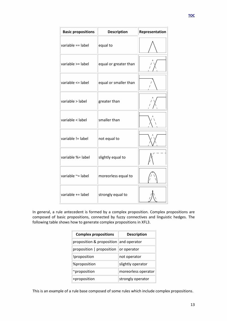
A basic proposition relates an input variable with one of its linguistic labels. XFL3 admits several relationships, such as equality, inequality and several linguistic hedges. The following table shows the different relationships offered by XFL3.

TOC

13

Basic propositions Description Representation

variable == label equal to

variable >= label equal or greater than

variable <= label equal or smaller than

variable > label greater than

variable < label smaller than

variable != label not equal to

variable %= label slightly equal to

variable ~= label moreorless equal to

variable += label strongly equal to

In general, a rule antecedent is formed by a complex proposition. Complex propositions are composed of basic propositions, connected by fuzzy connectives and linguistic hedges. The following table shows how to generate complex propositions in XFL3.

Complex propositions Description

proposition & proposition and operator

proposition | proposition or operator

!proposition not operator

%proposition slightly operator

~proposition moreorless operator

+proposition strongly operator

This is an example of a rule base composed of some rules which include complex propositions.

TOC

14

rulebase base1(input1 x, input2 y : output z) using systemop {

if( x == medium & y == medium) -> z = tall;

[0.8] if( x <=short | y != very_tall ) -> z = short;

if( +(x > tall) & (y ~= medium) ) -> z = tall;

............. }

Crisp blocks

A crisp block is a module which describes a non-fuzzy operation among some variables. In general, they use to be single operation such as sum, difference, product, etc. This kind of mathematical operations are commonly found in real problems where system variables needs to be combined in some way to adapt them to be used by a rulebase or to generate the output values of the system.

Crisp block definitions are encapsulated into a XFL3 object called crisp. Only one object crisp may appear in a system specification. The definition format of the object crisp in XFL3 is as follows:

The format of the crisp_function identifier is similar to the operator identifier, that is, "package.function" or simply "function" if the package which contains the definition of the crisp function has been already imported:

crisp {

difference xfl.diff2();

summation xfl.addN(3);

}

System global behavior

The description of the system global behavior means to define the global input and output variables of the system as well as the modular hierarchy. This description is as follows in XFL3:

The definition format of the global input and output variables is the same format employed in the definition of the rule bases. The inner variables that may appear establish serial or parallel interconnections among the modules. Inner variables must firstly appear as output variables of a module before being employed as input variables of other modules. Modules can refer to rule bases or to crisp blocks.

crisp {

identifier crisp_function(parameter_list);

identifier crisp_function(parameter_list);

............. }

system (input_list : output_list) {

rule_base_identifier(inputs : outputs);

rule_base_identifier(inputs : outputs);

............. }

TOC

15

system (Type1 x, Type2 y : Type3 z) {

rulebase1( x, y : inner1);

rulebase2( x, y : inner2);

rulebase3(inner1, inner2 : z);

}

Function packages

A great advantage of XFL3 is that functions assigned to fuzzy operators can be defined freely by the user in external files (named as packages), which gives a huge flexibility to the environment. Each package can include an unlimited number of definitions.

Six types of functions can be defined in XFL3: binary functions that can be used as T-norms, S-norms, and implication functions; unary functions that are related with linguistic hedges; crisp functions that implement crisp blocks; membership functions that are used to describe linguistic labels; families of membership functions that define a set of membership functions which share their parameters; and defuzzification methods.

A function definition include its name (and possible alias), the parameters that specify its behavior as well as the constraints on these parameters, the description of its behavior in the different languages to which it could be compiled (C, C++ and Java), and even the description of its differential function (if it is employed in gradient-based learning mechanisms). This information is the basis to generate automatically a Java class that incorporates all the function capabilities and can be employed by any XFL3 specification.

Definición de funciones binarias

Binary functions can be assigned to the conjunction operator (and), the disjunction operator (or), the implication function (imp), and the rule aggregation operator (also). The structure of a binary function definition in a function package is as follows:

binary identifier { blocks }

The blocks that can appear in a binary function definition are alias, parameter, requires, java, ansi_c, cplusplus, derivative and source.

The block alias is used to define alternative names to identify the function. Any of these identifiers can be used to refer the function. The syntax of the block alias is:

alias identifier, identifier, ... ;

The block parameter allows the definition of those parameters which the function depends on. The last identifier can be followed by brackets to define a list of parameters. Its format is:

parameter identifier, identifier, ... ;

TOC

16

The block requires expresses the constraints on the parameter values by means of a Java Boolean expression that validates the parameter values. The structure of this block is:

requires { expression }

The blocks java, ansi_c and cplusplus describe the function behavior by means of its description as a function body in Java, C and C++ programming languages, respectively. Input variables for these functions are 'a' and 'b'. The format of these blocks is the following:

java { Java_function_body }

ansi_c { C_function_body }

cplusplus { C++_function_body }

The block derivative describes the derivative function with respect to the input variables 'a' and 'b'. This description consists of a Java assignation expression to the variable 'deriv[]'. The derivative function with respect to the input variable 'a' must be assigned to 'deriv[0]', while the derivative function with respect to the input variable 'b' must be assigned to 'deriv[1]'. The description of the derivative function allows to propagate the system error derivative used by the supervised learning algorithms based on gradient descent. The format is:

derivative { Java_expressions }

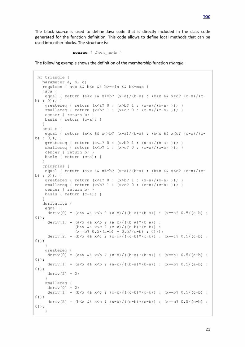
The block source is used to define Java code that is directly included in the class code generated for the function definition. This code allows to define local methods that can be used into other blocks. The structure is:

source { Java_code }

The following example shows the definition of the T-norm minimum, also used as Mamdani's implication function.

binary min {

alias mamdani;

java { return (a<b? a : b); }

ansi_c { return (a<b? a : b); }

cplusplus { return (a<b? a : b); }

derivative {

deriv[0] = (a<b? 1: (a==b? 0.5 : 0));

deriv[1] = (a>b? 1: (a==b? 0.5 : 0));

}

}

Unary function definition

Unary functions are used to describe the linguistic hedges. These functions can be assigned to the not modifier, the very or strongly modifier, the more-or-less modifier, and the slightly modifier. The structure of a unary function definition in a function package is as follows:

unary identifier { blocks }

The blocks that can appear in a unary function definition are alias, parameter, requires, java, ansi_c, cplusplus, derivative and source.

TOC

17







The blocks java, ansi_c and cplusplus describe the function behavior by means of its description as a function body in Java, C and C++ programming languages, respectively. Input variable for these functions is 'a'. The format of these blocks is the following:




The block derivative describes the derivative function with respect to the input variable 'a'. This description consists of a Java assignation expression to the variable 'deriv'. The description of the derivative function allows to propagate the system error derivative used by the supervised learning algorithms based on gradient descent. The format is:

derivative { Java_expressions }



The following example shows the definition of the Yager C-norm, which depends on the parameter w.

unary yager {

parameter w;

requires { w>0 }

java { return Math.pow( ( 1 - Math.pow(a,w) ) , 1/w ); }

ansi_c { return pow( ( 1 - pow(a,w) ) , 1/w ); }

cplusplus { return pow( ( 1 - pow(a,w) ) , 1/w ); }

derivative { deriv = - Math.pow( Math.pow(a,-w) -1, (1-w)/w ); }

}

TOC

18

Crisp function definition

Crisp functions are used to describe mathematical operations among variables with non-fuzzy values. These functions can be assigned to crisp modules which can be included in the modular hierarchy of fuzzy systems. The structure of a crisp function definition in a function package is as follows: crisp identifier { blocks }

The blocks that can appear in a crisp function definition are alias, parameter, requires, inputs, java, ansi_c, cplusplus and source.




parameter identifier, identifier, ..., identifier[] ;



The block inputs defines the number of input variables of the crisp function by means of a Java expresion which must return an integer value. The syntax of this block is:

inputs { Java_function_body }

The blocks java, ansi_c and cplusplus describe the function behavior by means of its description as a function body in Java, C and C++ programming languages, respectively. The variable 'x[]' contains the values of the input variables. The format of these blocks is the following:






The following example shows the definition of a crisp function which sums N input

values.

TOC

19

crisp addN {

parameter N;

requires { N>0 }

inputs { return (int) N; }

java {

double a = 0;

for(int i=0; i<N; i++) a+=x[i];

return a;

}

ansi_c {

int i;

double a = 0;

for(i=0; i<N; i++) a+=x[i];

return a;

}

cplusplus {

double a = 0;

for(int i=0; i<N; i++) a+=x[i];

return a;

}

}

Membership function definition

The membership functions are assigned to the linguistic labels that form a linguistic variable type. The structure of a membership function definition in a function package is as follows:

mf identifier { blocks }

The blocks that can appear in a membership function definition are alias, parameter, requires, java, ansi_c, cplusplus, derivative, update and source.





The block requires expresses the constraints on the parameter values by means of a Java Boolean expression that validates the parameter values. This expression can also use the values of the variables 'min' and 'max', which represent the minimum and maximum values in the universe of discourse of the linguistic variable considered. The structure of this block is:


The blocks java, ansi_c and cplusplus describe the function behavior by means of its description as a function body in Java, C and C++ programming languages, respectively. The format of these blocks is the following:

TOC

20




The definition of a membership function includes not only the description of the function behavior itself, but also the function behavior under the greater-or-equal and smaller-or-equal modifications, and the computation of the center and basis values of the membership function. As a consequence, the blocks java, ansi_c and cplusplus are divided into the following subblocks:

equal { code }

greatereq { code }

smallereq { code }

center { code }

basis { code }

The subblock equal describes the function behavior. The subblocks greatereq and smallereq describe the greater-or-equal and smaller-or-equal modifications, respectively. The input variable in these subblocks is called 'x', and the code can use the values of the function parameters and the variables 'min' and 'max', which represent the minimum and maximum values of the universe of discourse of the function. The subblocks greatereq and smallereq can be omitted. In that case, these transformations are computed by sweeping all the values of the universe of discourse. However, it is much more efficient to use an analytical function, so that the definition of these subblocks is strongly recommended.

The subblocks center and basis describe the center and basis of the membership function. The code of these subblocks can use the values of the function parameters and the variables 'min' and 'max'. This information is used by several simplified defuzzification methods. These subblocks are optional and their default functions return a zero value.

The block derivative describes the derivative function with respect to each function parameter. This block is also divided into the subblocks equal, greatereq, smallereq, center and basis. The code of these subblocks consists of Java expressions assigning values to the variable 'deriv[]'. The value of 'deriv[i]' represents the derivative of each function with respect to the i-th parameter of the membership function. The description of the derivative function allows to compute the system error derivative used by gradient descent-based learning algorithms. The format is:

derivative { subblocks }

The block update is used to compute a valid set of parameter values (stored in the variable pos[]) from a tainting displacement (stored in the variable disp[]) generated in an automatic tuning process, taking into account which of the parameters are intended to be modified (stored in the boolean variable adj[]). A very common constraint in the displacement is to maintain the order of the parameters. The preprogrammed function sortedUpdate(pos,disp,adj) can be invoked to compute this restricted displacement. The Java code can also use the variables min', 'max' and 'step', which represent respectively the minimum, maximum and division of the universe of discourse. The syntax of the block update is:

update { Java_function_body }

TOC

21



The following example shows the definition of the membership function triangle.

mf triangle {

parameter a, b, c;

requires { a<b && b<c && b>=min && b<=max }

java {

equal { return (a<x && x<=b? (x-a)/(b-a) : (b<x && x<c? (c-x)/(c-

b) : 0)); }

greatereq { return (x<a? 0 : (x>b? 1 : (x-a)/(b-a) )); }

smallereq { return (x<b? 1 : (x>c? 0 : (c-x)/(c-b) )); }

center { return b; }

basis { return (c-a); }

}

ansi_c {


b) : 0)); }





}

cplusplus {


b) : 0)); }





}

derivative {

equal {

deriv[0] = (a<x && x<b ? (x-b)/((b-a)*(b-a)) : (x==a? 0.5/(a-b) :

0));

deriv[1] = (a<x && x<b ? (a-x)/((b-a)*(b-a)) :

(b<x && x<c ? (c-x)/((c-b)*(c-b)) :

(x==b? 0.5/(a-b) + 0.5/(c-b) : 0)));

deriv[2] = (b<x && x<c ? (x-b)/((c-b)*(c-b)) : (x==c? 0.5/(c-b) :

0));

}

greatereq {

deriv[0] = (a<x && x<b ? (x-b)/((b-a)*(b-a)) : (x==a? 0.5/(a-b) :

0));

deriv[1] = (a<x && x<b ? (a-x)/((b-a)*(b-a)) : (x==b? 0.5/(a-b) :

0));

deriv[2] = 0;

}

smallereq {

deriv[0] = 0;

deriv[1] = (b<x && x<c ? (c-x)/((c-b)*(c-b)) : (x==b? 0.5/(c-b) :

0));

deriv[2] = (b<x && x<c ? (x-b)/((c-b)*(c-b)) : (x==c? 0.5/(c-b) :

0));

}

TOC

22

center {

deriv[0] = 1;

deriv[1] = 1;

deriv[2] = 1;

}

basis {

deriv[0] = -1;

deriv[1] = 0;

deriv[2] = 1;

}

}

update {

pos = sortedUpdate(pos,desp,adj);

if(pos[1]<min) pos[1]=min;

if(pos[2]<=pos[1]) pos[2] = pos[1]+step;

if(pos[1]>max) pos[1]=max;

if(pos[0]>=pos[1]) pos[0] = pos[1]-step;

}

}

Membership function family definition

A family of membership functions describes a set of membership functions that shares a list of parameters. Families are used to define sets of membership functions with certain constraints such as symmetrical membership functions, a fixed overlapping degree or a fixed order. Each membership function is referenced by its index on the family. The structure of the definition of a membership function family in a function package is as follows:

family identifier { blocks }

The blocks that can appear in a family definition are alias, parameter, requires, members, java, ansi_c, cplusplus, derivative, update and source.

The block alias is used to define alternative names to identify the family. Any of these identifiers can be used to refer the family. The syntax of the block alias is:


The block parameter allows the definition of those parameters which the family depends on. The last identifier can be followed by brackets to define a list of parameters. Its format is:


The block requires expresses the constraints on the parameter values by means of a Java Boolean expression that validates the parameter values. This expression can also use the values of the variables 'min' and 'max', which represent the minimum and maximum values in the universe of discourse of the linguistic variable considered. The structure of this block is:


The block members defines the number of membership functions of the family by means of a Java expression which must return an integer value. The syntax of this block is:

TOC

23

members { Java_function_body }

The blocks java, ansi_c and cplusplus describe the functions behavior by means of its description as a function body in Java, C and C++ programming languages, respectively. The format of these blocks is the following:




The definition of a family of membership functions includes not only the description of the functions behavior itself, but also the functions behavior under the greater-or-equal and smaller-or-equal modifications, and the computation of the center and basis values of the membership functions. As a consequence, the blocks java, ansi_c and cplusplus are divided into the following subblocks:

equal { code }

greatereq { code }

smallereq { code }

center { code }

basis { code }

The subblock equal describes the function behavior. The subblocks greatereq and smallereq describe the greater-or-equal and smaller-or-equal modifications, respectively. The variable 'i' is used to identify the index of the membership function in the family. The input variable in these subblocks is called 'x', and the code can use the values of the family parameters and the variables 'min' and 'max', which represent the minimum and maximum values of the universe of discourse of the family. The subblocks greatereq and smallereq can be omitted. In that case, these transformations are computed by sweeping all the values of the universe of discourse. However, it is much more efficient to use an analytical function, so that the definition of these subblocks is strongly recommended.

The subblocks center and basis describe the center and basis of the membership functions. The code of these subblocks can use the values of the variable 'i' (the index of the membership function), the family parameters and the variables 'min' and 'max'. This information is used by several simplified defuzzification methods. These subblocks are optional and their default functions return a zero value.

The block derivative describes the derivative of each function with respect to each family parameter. This block is also divided into the subblocks equal, greatereq, smallereq, center and basis. The code of these subblocks consists of Java expressions assigning values to the variable 'deriv[]'. The value of 'deriv[j]' represents the derivative of each function with respect to the j-th parameter of the family. The description of the derivative function allows to compute the system error derivative used by gradient descent-based learning algorithms. The format is:

derivative { subblocks }

The block update is used to compute a valid set of parameter values (stored in the variable pos[]) from a tainting displacement (stored in the variable disp[]) generated in an automatic tuning process, taking into account which of the parameters are intended to be modified (stored in the boolean variable adj[]). A very common constraint in the displacement is to maintain the order of the parameters. The preprogrammed function sortedUpdate(pos,disp,adj) can be invoked to compute this restricted displacement. The Java

TOC

24

code can also use the variables min', 'max' and 'step', which represent respectively the minimum, maximum and division of the universe of discourse. The syntax of the block update is:

update { Java_function_body }



The following example shows the definition of the membership function family triangular.

family triangular {

parameter p[];

requires { p.length==0 || (p.length>0 && p[0]>min && p[p.length-

1]<max && sorted(p)) }

members { return p.length+2; }

java {

equal {

double a = (i==0? min-1 : (i==1 ? min : p[i-2]));

double b = (i==0? min : (i==p.length+1? max : p[i-1]));

double c = (i==p.length? max : (i==p.length+1? max+1 : p[i]));

return (a<x && x<=b? (x-a)/(b-a) : (b<x && x<c? (c-x)/(c-b): 0));

}

greatereq {



return (x<a? 0 : (x>b? 1 : (x-a)/(b-a) ));

}

smallereq {



return (x<b? 1 : (x>c? 0 : (c-x)/(c-b) ));

}

center {


return b;

}

basis {

double a = (i<=1 ? min : p[i-2]);

double c = (i>=p.length? max : p[i]);

return (c-a);

}

}

ansi_c {

equal {


double b = (i==0? min : (i==length+1? max : p[i-1]));

double c = (i==length? max : (i==length+1? max+1 : p[i]));


}

greatereq {



return (x<a? 0 : (x>b? 1 : (x-a)/(b-a) ));

}

TOC

25

smallereq {



return (x<b? 1 : (x>c? 0 : (c-x)/(c-b) ));

}

center {


return b;

}

basis {

double a = (i<=1 ? min : p[i-2]);

double c = (i>=length? max : p[i]);

return (c-a);

}

}

cplusplus {

equal {





}

greatereq {



return (x<a? 0 : (x>b? 1 : (x-a)/(b-a) ));

}

smallereq {



return (x<b? 1 : (x>c? 0 : (c-x)/(c-b) ));

}

center {


return b;

}

basis {

double a = (i<=1 ? min : p[i-2]);

double c = (i>=length? max : p[i]);

return (c-a);

}

}

derivative {

equal {




if(i>=2) {

if(a<x && x<b) deriv[i-2] = (x-b)/((b-a)*(b-a));

else if(x==a) deriv[i-2] = 0.5/(a-b);

else deriv[i-2] = 0;

}

if(i>=1 && i<=p.length) {

if(a<x && x<b) deriv[i-1] = (a-x)/((b-a)*(b-a));

else if(b<x && x<c) deriv[i-1] = (c-x)/((c-b)*(c-b));

else if(x==b) deriv[i-1] = 0.5/(a-b) + 0.5/(c-b);


}

if(i<p.length) {

if(b<x && x<c) deriv[i] = (x-b)/((c-b)*(c-b));

TOC

26

else if(x==c) deriv[i] = 0.5/(c-b);

else deriv[i] = 0;

}

}

greatereq {



if(i>=2) {

if(a<x && x<b) deriv[i-2] = (x-b)/((b-a)*(b-a));

else if(x==a) deriv[i-2] = 0.5/(a-b);


}


if(a<x && x<b) deriv[i-1] = (a-x)/((b-a)*(b-a));

else if(x==b) deriv[i-1] = 0.5/(a-b);


}

}

smallereq {




if(b<x && x<c) deriv[i-1] = (c-x)/((c-b)*(c-b));

else if(x==b) deriv[i-1] = 0.5/(c-b);


}

if(i<p.length) {

if(b<x && x<c) deriv[i] = (x-b)/((c-b)*(c-b));

else if(x==c) deriv[i] = 0.5/(c-b);

else deriv[i] = 0;

}

}

center {

if(i>=1 && i<=p.length) deriv[i-1] = 1;

}

basis {

if(i>1) deriv[i-2] = -1;

if(i<p.length) deriv[i] = 1;

}

}

update {

if(p.length == 0) return;

pos = sortedUpdate(pos,desp,adj);

if(pos[0]<=min) {

pos[0]=min+step;

for(int i=1;i<p.length; i++) {

if(pos[i]<=pos[i-1]) pos[i] = pos[i-1]+step;

else break;

}

}

if(pos[p.length-1]>=max) {

pos[p.length-1]=max-step;

for(int i=p.length-2; i>=0; i--) {

if(pos[i]>=pos[i+1]) pos[i] = pos[i+1]-step;

else break;

}

}

}

}

TOC

27

Defuzzification method definition

Defuzzification methods obtain the representative value of a fuzzy set. These methods are used in the final stage of the fuzzy inference process, when it is not possible to work with fuzzy conclusions. The structure of a defuzzification method definition in a function package is as follows:

defuz identifier { blocks }

The blocks that can appear in a defuzzification method definition are alias, parameter, requires, definedfor, java, ansi_c, cplusplus and source.

The block alias is used to define alternative names to identify the method. Any of these identifiers can be used to refer the method. The syntax of the block alias is:


The block parameter allows the definition of those parameters which the method depends on. Its format is:




The block definedfor is used to enumerate the types of membership functions that the method can use as partial conclusions. This block has been included because some simplified defuzzification methods only work with certain membership functions. This block is optional. By default, the method is assumed to work with all the membership functions. The structure of the block is:

definedfor identificador, identificador, ... ;

The block source is used to define Java code that is directly included in the class code generated for the method definition. This code allows to define local functions that can be used into other blocks. The structure is:


The blocks java, ansi_c and cplusplus describe the behavior of the method by means of its description as a function body in Java, C and C++ programming languages, respectively. The format of these blocks is the following:




The input variable for these functions is the object 'mf', which encapsulates the fuzzy set obtained as the conclusion of the inference process. The code can use the value of the variables 'min', 'max' and 'step', which represent respectively the minimum, maximum and division of the universe of discourse of the fuzzy set. Conventional defuzzification methods are based on sweeps along all the values of the universe of discourse, and they compute the

TOC

28

membership degree of each value in the universe. On the other side, simplified defuzzification methods use sweeps along the partial conclusions, and they compute the representative value in terms of the activation degree, center, basis and parameters of these partial conclusions. The way this information is accessed by the object mf depends on the programming language, as shown in the next table.

Description java ansi_c cplusplus

membership degree mf.compute(x) mf.compute(x) mf.compute(x)

partial conclusions mf.conc[] mf.conc[] mf.conc[]

number of partial conclusions mf.conc.length mf.length mf.length

activation degree of the i-th conclusion

mf.conc[i].degree() mf.degree[i] mf.conc[i]->degree()

center of the i-th conclusion mf.conc[i].center() center(mf.conc[i]) mf.conc[i]->center()

basis of the i-th conclusion mf.conc[i].basis() basis(mf.conc[i]) mf.conc[i]->basis()

j-th parameter of the i-th conclusion

mf.conc[i].param(j) param(mf.conc[i],j) mf.conc[i]->param(j)

number of the input variables in the rule base

mf.input.length mf.inputlength mf.inputlength

values of the input variables in the rule base

mf.input[] mf.input[] mf.input[]

The following example shows the definition of the classical CenterOfArea defuzzification method.

defuz CenterOfArea {

alias CenterOfGravity, Centroid;

java {

double num=0, denom=0;

for(double x=min; x<=max; x+=step) {

double m = mf.compute(x);

num += x*m;

denom += m;

}

if(denom==0) return (min+max)/2;

return num/denom;

}

ansi_c {

double x, m, num=0, denom=0;

for(x=min; x<=max; x+=step) {

m = compute(mf,x);

num += x*m;

denom += m;

}


return num/denom;

}

cplusplus {


TOC

29

for(double x=min; x<=max; x+=step) {

double m = mf.compute(x);

num += x*m;

denom += m;

}


return num/denom;

}

}

The following example shows the definition of a simplified defuzzification method (Weighted Fuzzy Mean).

defuz WeightedFuzzyMean {

definedfor triangle, isosceles, trapezoid, bell, rectangle;

java {


for(int i=0; i<mf.conc.length; i++) {

num += mf.conc[i].degree()*mf.conc[i].basis()*mf.conc[i].center();

denom += mf.conc[i].degree()*mf.conc[i].basis();

}


return num/denom;

}

ansi_c {


int i;

for(i=0; i<mf.length; i++) {

num += mf.degree[i]*basis(mf.conc[i])*center(mf.conc[i]);

denom += mf.degree[i]*basis(mf.conc[i]);

}


return num/denom;

}

cplusplus {


for(int i=0; i<mf.length; i++) {

num += mf.conc[i]->degree()*mf.conc[i]->basis()*mf.conc[i]-

>center();

denom += mf.conc[i]->degree()*mf.conc[i]->basis();

}


return num/denom;

}

}

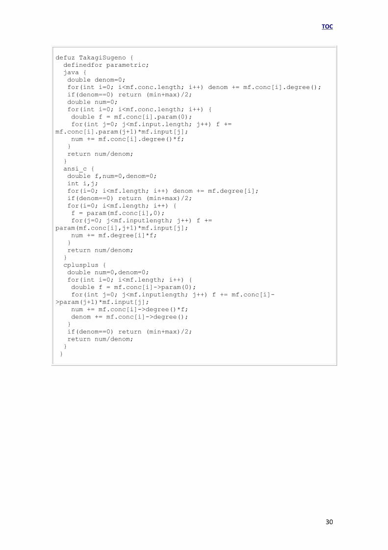
Este último ejemplo muestra la definición del método de Takagi-Sugeno de primer orden.

TOC

30

defuz TakagiSugeno {

definedfor parametric;

java {

double denom=0;

for(int i=0; i<mf.conc.length; i++) denom += mf.conc[i].degree();


double num=0;

for(int i=0; i<mf.conc.length; i++) {

double f = mf.conc[i].param(0);

for(int j=0; j<mf.input.length; j++) f +=

mf.conc[i].param(j+1)*mf.input[j];

num += mf.conc[i].degree()*f;

}

return num/denom;

}

ansi_c {

double f,num=0,denom=0;

int i,j;

for(i=0; i<mf.length; i++) denom += mf.degree[i];


for(i=0; i<mf.length; i++) {

f = param(mf.conc[i],0);

for(j=0; j<mf.inputlength; j++) f +=

param(mf.conc[i],j+1)*mf.input[j];

num += mf.degree[i]*f;

}

return num/denom;

}

cplusplus {

double num=0,denom=0;

for(int i=0; i<mf.length; i++) {

double f = mf.conc[i]->param(0);

for(int j=0; j<mf.inputlength; j++) f += mf.conc[i]-

>param(j+1)*mf.input[j];

num += mf.conc[i]->degree()*f;

denom += mf.conc[i]->degree();

}


return num/denom;

}

}

TOC

31

The standard package xfl

The XFL3 specification language allows the user to define its own membership functions, families of membership functions, crisp functions, defuzzification methods, and functions related with fuzzy connectives and linguistic hedges. In order to ease the use of XFL3, the most well-known functions have been included in a standard package called xfl. The binary functions included are the following:

Name Type Java description

min T-norm (a<b? a : b)

prod T-norm (a*b)

bounded_prod T-norm (a+b-1>0? a+b-1: 0)

drastic_prod T-norm (a==1? b: (b==1? a : 0) )

max S-norm (a>b? a : b)

sum S-norm (a+b-a*b)

bounded_sum S-norm (a+b<1? a+b: 1)

drastic_sum S-norm (a==0? b : (b==0? a : 0) )

dienes_resher Implication (b>1-a? b : 1-a)

mizumoto Implication (1-a+a*b)

lukasiewicz Implication (b<a? 1-a+b : 1)

dubois_prade Implication (b==0? 1-a : (a==1? b : 1) )

zadeh Implication (a<0.5 || 1-a>b? 1-a : (a<b? a : b))

goguen Implication (a<b? 1 : b/a)

godel Implication (a<=b? 1 : b)

sharp Implication (a<=b? 1 : 0)

The unary functions included in the package xfl are:

Name Parameter Java description

not - (1-a)

sugeno l (1-a)/(1+a*l)

square - (a*a)

cubic - (a*a*a)

sqrt - Math.sqrt(a)

yager w Math.pow( ( 1 - Math.pow(a,w) ) , 1/w )

pow w Math.pow(a,w)

parabola - 4*a*(1-a)

edge - (a<=0.5? 2*a : 2*(1-a) )

TOC

32

The crisp functions included in the package xfl are:

Name Parameter Description

add2 - Suma de variables

addN N Suma de N variables

addDeg - Suma de dos variables angulares (en grados)

addRad - Suma de dos variables angulares (en radianes)

diff2 - Diferencia entre dos variables

diffDeg - Diferencia entre dos variables angulares (en grados)

diffRad - Diferencia entre dos variables ngulares (en radianes)

prod - Producto de dos variables

div - División entre dos variables

select N Selección entre N variables

The membership functions defined in the package xfl are the following:

Name Parameters Description

triangle a,b,c

trapezoid a,b,c,d

isosceles a,b

slope a,m

bell a,b

TOC

33

sigma a,b

rectangle a,b

singleton a

parametric unlimited -

The families of membership functions defined in the package xfl are the following:

Name Parameters Description

rectangular p[]

triangular p[]

sh_triangular p[]

spline p[]

TOC

34

The defuzzification methods defined in the standard package are:

Name Type Defined for

CenterOfArea Conventional any function

FirstOfMaxima Conventional any function

LastOfMaxima Conventional any function

MeanOfMaxima Conventional any function

FuzzyMean Simplified triangle, isosceles, trapezoid, bell, rectangle, singleton

WeightedFuzzyMean Simplified triangle, isosceles, trapezoid, bell, rectangle

Quality Simplified triangle, isosceles, trapezoid, bell, rectangle

GammaQuality Simplified triangle, isosceles, trapezoid, bell, rectangle

MaxLabel Simplified singleton

TakagiSugeno Simplified parametric

TOC

35

The Xfuzzy 3 development environment

The Xfuzzy 3 development environment o Description stage

System edition (xfedit) Package edition (xfpkg)

o Verification Stage Graphical representation (xfplot) Inference monitor (xfmt) System simulation (xfsim)

o Tuning stage Knowledge acquisition (xfdm) Time series prediction (xftsp) Supervised learning (xfsl) Simplification (xfsp)

o Synthesis stage C code generator (xfc) C++ code generator (xfcpp) Java code generator (xfj) VHDL code generator code generator (xfvhdl) SysGen model generator (xfsg)

Xfuzzy 3 is a development environment for designing fuzzy systems, which integrates several tools covering the different stages of the design. The environment integrates all these tools under a graphical user interface which eases the design process. The next figure shows the main window of the environment.

TOC

36

The menu bar in the main window contains the links to the different tools. Under the menu bar, there is a button bar with the most used options. The central zone of the window shows two lists. The first one is the list of loaded systems (the environment can work with several systems simultaneously). The second list contains the loaded packages. The rest of the main window is occupied by a message area.

The menu bar is divided into the different stages of the system development. The File menu allows to create, load, save and close a fuzzy system. This menu contains also the options to create, load, save and close a function package. The menu ends with the option to exit the environment. The Design menu is used to edit a selected fuzzy system (xfedit) or a selected package (xfpkg). The Tuning menu contains the links to the knowledge acquisition tool (xfdm), the time series prediction tool (xftsp), the supervised learning tool (xfsl), and the simplification tool (xfsp). The Verification menu allows to represent the system behavior on a 2-dimensional or 3-dimensional plot (xfplot), monitoring the system (xfmt), and simulating it (xfsim). The Synthesis menu is divided into two parts: the software synthesis, that generates system descriptions in C (xfc), C++ (xfcpp), and Java (xfj); and the hardware synthesis, that translates the description of a fuzzy system into VHDL code (xfvhdl) or a Simulink model for Xilinx's SysGen tool (xfsg). The Set Up menu is used to modify the environment working directory, to save the environment messages in an external log file, to close the log file, to clean up the message area of the main window, and to change the look and feel of the environment.

Many options on the menu bar are only enabled when a fuzzy system is selected. A fuzzy system is selected by just clicking its name in the system list. Double clicking the name will open the edition tool. The same result is obtained by pressing the Enter key once the system has been selected. The Insert key will create a new system and the Delete key is used to close the system. These shortcuts are common to all the lists of the environment: the Insert key is used to insert a new element on a list; the Enter key or a double click will edit the selected element; and the Delete key will remove the element from the list.

Description stage

The first step in the development of a fuzzy system is to select a preliminary description of the system. This description will be later refined as a result of the tuning and verification stages.

Xfuzzy 3 contains two tools assisting in the description of fuzzy systems: xfedit and xfpkg. The first one is dedicated to the logical definition of the system, that is, the definition of its linguistic variables and the logical relations between them. On the other side, the xfpkg tool eases the description of the mathematical functions assigned to the fuzzy operators, linguistic hedges, membership functions and defuzzification methods.

TOC

37

The system edition tool – Xfedit

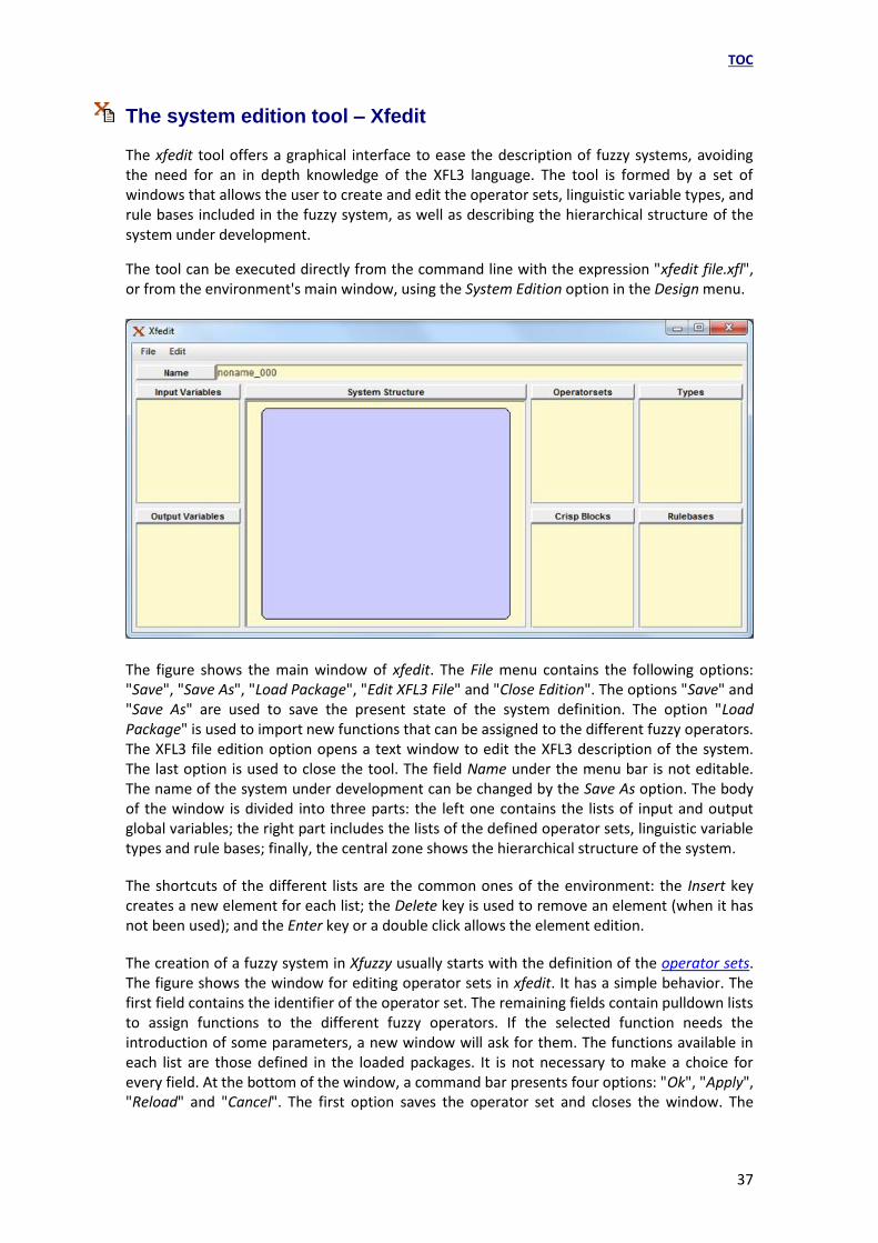
The xfedit tool offers a graphical interface to ease the description of fuzzy systems, avoiding the need for an in depth knowledge of the XFL3 language. The tool is formed by a set of windows that allows the user to create and edit the operator sets, linguistic variable types, and rule bases included in the fuzzy system, as well as describing the hierarchical structure of the system under development.

The tool can be executed directly from the command line with the expression "xfedit file.xfl", or from the environment's main window, using the System Edition option in the Design menu.

The figure shows the main window of xfedit. The File menu contains the following options: "Save", "Save As", "Load Package", "Edit XFL3 File" and "Close Edition". The options "Save" and "Save As" are used to save the present state of the system definition. The option "Load Package" is used to import new functions that can be assigned to the different fuzzy operators. The XFL3 file edition option opens a text window to edit the XFL3 description of the system. The last option is used to close the tool. The field Name under the menu bar is not editable. The name of the system under development can be changed by the Save As option. The body of the window is divided into three parts: the left one contains the lists of input and output global variables; the right part includes the lists of the defined operator sets, linguistic variable types and rule bases; finally, the central zone shows the hierarchical structure of the system.

The shortcuts of the different lists are the common ones of the environment: the Insert key creates a new element for each list; the Delete key is used to remove an element (when it has not been used); and the Enter key or a double click allows the element edition.

The creation of a fuzzy system in Xfuzzy usually starts with the definition of the operator sets. The figure shows the window for editing operator sets in xfedit. It has a simple behavior. The first field contains the identifier of the operator set. The remaining fields contain pulldown lists to assign functions to the different fuzzy operators. If the selected function needs the introduction of some parameters, a new window will ask for them. The functions available in each list are those defined in the loaded packages. It is not necessary to make a choice for every field. At the bottom of the window, a command bar presents four options: "Ok", "Apply", "Reload" and "Cancel". The first option saves the operator set and closes the window. The

TOC

38

second one just saves the last changes. The third option actualizes the field with the last saved values. The last one closes the window rejecting the last changes.

The following step in the description of a fuzzy system is to create the linguistic variable types, by means of the Type Creation window shown below. A new type needs the introduction of its identifier and universe of discourse (minimum, maximum and cardinality). The window includes several predefined types corresponding to the most usual partitions of the universes. These predefined types contain homogeneous triangular, trapezoidal, bell-shaped and singleton partitions, shouldered-triangular and shouldered-bell partitions. Other predefined types are equal bells and singletons, which are commonly used as a first option for output variable types. When one of the previous predefined types is selected, the number of membership function of the partition must be introduced. The predefined types also include a blank option, which generates a type without any membership function, and the extension of an existing type (selected in the Parent field), that implements the inheritance mechanism of XFL3.

Once a type has been created, it can be edited using the Type Edition window. This window allows the modification of the type name and universe of discourse, for instance by adding, editing and removing the membership functions of the edited type. The window shows a graphical representation of the membership functions, where the selected membership function is represented in a different color. The bottom of the window presents a command bar with the usual buttons to save or reject the last changes, and to close the window. It is worth considering that the modifications on the definition of the universe of discourse can affect the membership functions. Hence, a validation of the membership function parameters

TOC

39

is done before saving the modifications, and an error message appear whenever a membership function definition becomes invalid.

A membership function can be created or edited from the MF list with the usual accelerators (Insert key and Enter key or double click). The previous figure shows the window for editing a membership function. The window has fields to introduce the name of the linguistic label, to select the kind of membership function, and to introduce the parameter values. The right side of the window shows a graphical representation of all the membership functions, with the function being edited shown in a different color. The bottom of the window shows a command bar with three options: Set, to close the window saving the changes, Refresh, to repaint the graphical representation, and Cancel, to close the window without saving the modifications.

The third step in the definition of a fuzzy system is to describe the rule bases expressing the relationship among the system variables. Rule bases can be created, edited and removed from their list with the usual shortcuts (Insert key, Enter key or double click, and Delete key). The following window eases the edition of the rule bases.

TOC

40

The rule base edition window is divided into three zones: the left side has the fields to introduce the names of the rule base and the operator set used, and to introduce the lists of input and output variables; the right zone is dedicated to showing the contents of the rules included in the rule base; and the bottom part of the window contains the command bar with the usual buttons to save or reject the modifications, and to close the window.

The input and output variables can be created, edited, or removed with the common list bindkeys. The information required by a variable definition is the name and the type of the variable.

The contents of the rules can be displayed in three formats: free, tabular, and matricial. The free format uses three fields for each rule. The first one contains the confidence weight. The second field shows the antecedent of the rule. This is an auto-editable field, where changes can be made by selecting the term to modify (a "?" symbol means a blank term) and by using the buttons of the window. The third field of each rule contains the consequent description. This is also an auto-editable field that can be modified by clicking the "->" button. New rules can be generated by introducing values on the last row (marked with the "*" symbol).

The button bar at the bottom of the free form allows to create conjunction terms ("&" button), disjunction terms ("|" button), modified terms with the linguistic hedges not ("!" button), more or less ("~" button), slightly ("%" button), and strongly ("+" button), and single terms relating a variable and a label with the clauses equal to ("=="), not equal to ("!="), greater than (">"), smaller than ("<"), greater or equal to (">="), smaller or equal to ("<="), approximately equal to ("~="), strongly equal to ("+="), and slightly equal to ("%="). The "->" button is used to add a rule conclusion. The ">..<" button is used to remove a conjunction or disjunction term (e.g. a term "v == l & ?" is transformed into "v == l"). The free form allows the user to describe more complex relationships among the variables than the other forms.

TOC

41

The tabular format is useful to define rules whose antecedent use only the operators and and equal. Each rule has a field to introduce the confidence weight and a pulldown list per input and output variables. There is no need of selecting all the variables fields, but one input and one output variables have always to be selected. If a rule base contains a rule that cannot be expressed in the tabular format, the table form can not be opened and an error message appears instead.

The matricial format is specially designed to describe a 2-input 1-output rule base. This form shows the content of a rule base in a clear and compact way. The matrix form generates rules such as "if(x==X & y==Y) -> z=Z", i.e., rules with a 1.0 confidence weight and formed by the conjunction of two equalities. Those rule bases that do not have the proper number of variables, or that contain rules with a different format, can not be shown in this form.

TOC

42

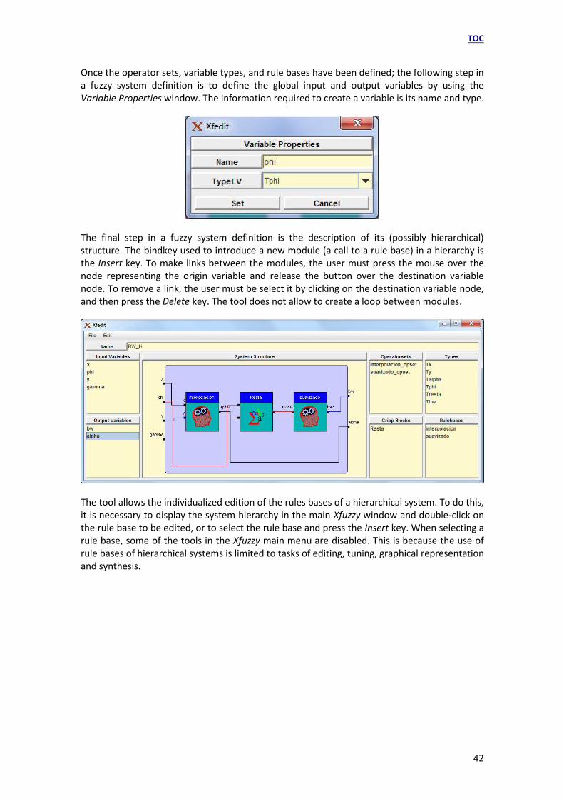
Once the operator sets, variable types, and rule bases have been defined; the following step in a fuzzy system definition is to define the global input and output variables by using the Variable Properties window. The information required to create a variable is its name and type.

The final step in a fuzzy system definition is the description of its (possibly hierarchical) structure. The bindkey used to introduce a new module (a call to a rule base) in a hierarchy is the Insert key. To make links between the modules, the user must press the mouse over the node representing the origin variable and release the button over the destination variable node. To remove a link, the user must be select it by clicking on the destination variable node, and then press the Delete key. The tool does not allow to create a loop between modules.

The tool allows the individualized edition of the rules bases of a hierarchical system. To do this, it is necessary to display the system hierarchy in the main Xfuzzy window and double-click on the rule base to be edited, or to select the rule base and press the Insert key. When selecting a rule base, some of the tools in the Xfuzzy main menu are disabled. This is because the use of rule bases of hierarchical systems is limited to tasks of editing, tuning, graphical representation and synthesis.

TOC

43

In the xfedit window it is possible to add new operator sets, change the types of the output variables and modify the rules.

The options enabled in the editing window work in a similar way to those used when editing the complete system. As an observation, it is convenient to add that to change the name of a rule base, you have to access the rule base edit window and change the name there.

TOC

44

The package edition tool – Xfpkg

The description of a fuzzy system within the Xfuzzy 3 environment is divided into two parts. The system logical structure (including the definitions of operator sets, variable types, rule bases, and hierarchical behavior structure) is specified in files with the extension ".xfl", and can be graphically edited with xfedit. On the other hand, the mathematical description of the functions used as fuzzy connectives, linguistic hedges, membership functions, families of membership functions, crisp blocks, and defuzzification methods are specified in packages.

The xfpkg tool is dedicated to easing the package edition. The tool implements a graphical user interface that shows the list of the different functions included in the package, and the contents of the different fields of a function definition. Most of these fields contains code describing the function in different programming languages. This code must be introduced manually. The tool can be executed from the command line or from the main window of the environment, using the option Edit package in the Design menu.

The previous figure shows the main window of xfpkg. The File menu contains the options "Save", "Save as", "Compile", "Delete" and "Close edition". The first two options are used to save the package file. The option "Compile" carries out a compilation process that generates the ".java" and ".class" files related to each function defined in the package. The option "Delete" is used to remove the package file and all the ".java" and ".class" files generated by the compilation process. The last option is used to close the tool.

The main window contains six lists showing the different kinds of functions included in the package: binary functions (related to conjunction, disjunction, aggregation, and implication operators), unary functions (associated with linguistic hedges), membership functions (related to linguistic labels), families of membership functions (used to describe a set of membership functions), crisp functions (associated with crisp blocks), and defuzzification methods (used to obtain representative values of the fuzzy conclusions).

A double click on any element of the lists will open the function definition window. This window shows the content of the different fields of a function definition. The bottom of this part contains a group of three buttons: "Edit", "Apply" and "Reload". When a function is selected in a list, its fields cannot be modified at first. The Edit command is used to allow the

TOC

45

user modifying the fields. The Apply command saves the changes of the definition. This includes the generation of the ".java" and ".class" files. The Reload command rejects the modifications and actualizes the fields with the previous values.

The fields of a function definition are distributed among eight tabbed panels. The Alias panel contains the list of alternative identifiers.

The Parameters panel contains the enumeration of the parameters used by the edited function.

The panel titled Requirements is used to describe the constraints on the parameter values.

TOC

46

The Java, C and C++ panels contain the description of the function behavior in these programming languages.

The Derivative panel contains the description of the derivative function.

TOC

47

The last panel contains the source block with the Java code of local methods that can be used in another fields and that are directly incorporated in the ".java" file.

The definition of a membership function or a family of membership functions requires additional information to describe the function behavior in the different programming languages. In these cases, the Java, C, C++ and Derivative panels contain five fields to show the contents of the subblocks equal, greatereq, smallereq, center, and basis.

In addition, the definition window for membership functions and families of membership functions also include an Update panel describing how to modify the values of the function parameters in terms of a set of displacements.

TOC

48

The definition of a family of membership functions contains an additional panel describing how to compute the number of functions included in that family.

Regarding defuzzification methods, they can include the enumeration of the membership functions that can be used by each method. This enumeration appears in the Requirements panel.

TOC

49

Finally, the window describing a crisp function includes an Inputs panel that defines the number of input variables of the function.

The xfpkg tool implements a graphical interface that allows the user to view and edit the definition of the functions included into a package file. This tool is used to describe the mathematical behavior of the defined functions in a graphical way. So, this tool is the complement of the xfedit tool, which describes the logical structure of the system, in the fuzzy system description stage.

TOC

50

Verification stage

The verification stage in the fuzzy system design process consists in studying the behavior of the fuzzy system under development. The aim of this stage is the detection of probable deviations on the expected behavior and the identification of the sources of these deviations.

The Xfuzzy environment covers the verification stage with three tools. The first one is xfplot, which shows the system behavior by a two-dimensional or three-dimensional plot. The monitor tool, xfmt, shows the activation degree of every linguistic label and logical rule, as well as the value of the different inner variables, for a given set of input values. The last tool, xfsim, is aimed at simulating the system within its actual or modeled operational environment. It allows illustrating the system evolution by means of a graphical representation of user-selected variables.

The graphical representation tool - Xfplot

The xfplot tool illustrates the behavior of a fuzzy system by a 2-dimensional or 3-dimensional representation. The tool can be executed from the command line with the expression "xfplot file.xfl", or from the main window of the environment, using the option "Graphical representation" in the Verification menu.

The main window of the tool is formed by a central panel, which shows the graphical representation, and an upper bar, dedicated to configuring the representation.

The File menu at the upper bar allows to save the represented data into an external file ("Save Data"), to save the graphical representation as an image (opción "Save image"), to refresh the graphical representation ("Actualize"), and to close the tool ("Close"). The Configuration menu is used to choose the kind of representation ("Plot Mode"), the colors of the plot ("Color Model"), and the values for the input variables ("Input Values"), so as to load a configuration from an external file ("Load Configuration") or to save the configuration into an external file ("Save Configuration"). Three pulldown lists allow the selection of the variables assigned to each axis. The last field contains the number of points used in the partition of the X and Y axis. This is an important parameter because it determines the representation resolution. A low value in this parameter can exclude important details of the system behavior. On the other

TOC

51

hand, a high value will make it difficult to understand the represented surface, as it will use a very dense grid. The default value of this parameter is 40.

The 3-dimensional representation includes the possibility of rotating the surface by using two sliding buttons at the right and bottom parts of the plot. This rotation capability eases the interpretation of the represented surface.

When choosing a 2-dimensional representation, the central panel changes to show a plain plot wich represents the variation of the output variable selected as Z axis, with respect to the input variable selected as X axis.

When the system under representation contains a number of input variables greater than the required by the kind of representation, it is necessary to introduce the values for the non-selected input variables. This can be done by the option "Input Values", which opens the following window.

TOC

52

The inference monitor tool – Xfmt

The aim of the xfmt tool is to monitor the fuzzy inference process in the system, i.e., to show graphically the values of the different inner variables and the activation degree of the logical rules and linguistic labels, for a given set of input values. The tool can be executed from the command line with the expression "xfmt file.xfl", or from the main window of the environment, using the option "Monitor" in the Verification menu.

The main window of xfmt is divided into three parts. The left zone is used to introduce the values of the global input variables. For each variable, there is a field to introduce manually its value, and a sliding button to introduce the value as a position within the variable range. The right side shows the fuzzy set associated with the value of the global output variables, as well as the crisp (defuzzified) value for that variable. This crisp value is also shown as a singleton in the plot of the fuzzy set (if the fuzzy set is already a singleton, this plot only shows this singleton). The center of the window illustrates the (hierarchical) structure of the system. .

The tool also includes a window to monitor the inner values of the inference process on each rule base. To open this window, just click on the rule base on the hierarchical structure of the system.

TOC

53

The rule base monitor window is divided into three parts. The values of the input variables are shown at the left as singleton values within the membership functions assigned to the different linguistic labels. The center of the window contains a set of fields with the activation degree of each rule. The right side shows the values of the output variables obtained by the inference process. If the operator set used in the rule base specifies a defuzzification method, the output value is defuzzified, and the variable plot shows not only the fuzzy value but also the crisp value that is finally assigned to the output variable.

This tool can be used to monitor the behavior of each of the rules bases of a hierarchical inference system (selecting each rule base before invoking xfmt). In this way it is possible to analyze the input/output behavior of a certain rule base by modifying values of internal variables of the system.

The simulation tool – Xfsim

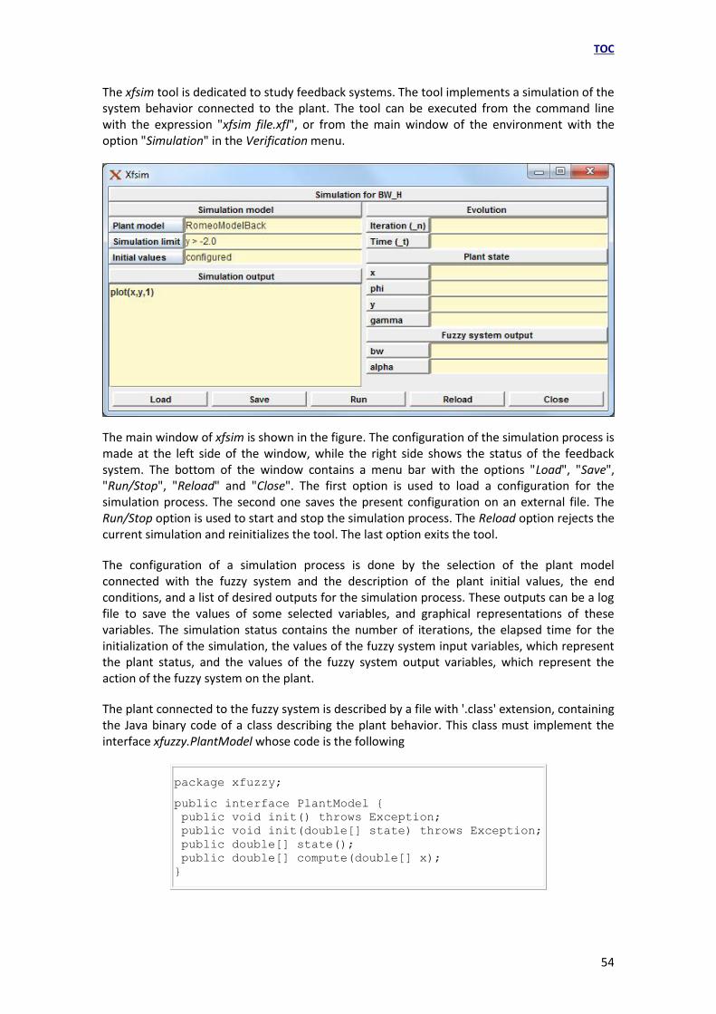
TOC

54

The xfsim tool is dedicated to study feedback systems. The tool implements a simulation of the system behavior connected to the plant. The tool can be executed from the command line with the expression "xfsim file.xfl", or from the main window of the environment with the option "Simulation" in the Verification menu.

The main window of xfsim is shown in the figure. The configuration of the simulation process is made at the left side of the window, while the right side shows the status of the feedback system. The bottom of the window contains a menu bar with the options "Load", "Save", "Run/Stop", "Reload" and "Close". The first option is used to load a configuration for the simulation process. The second one saves the present configuration on an external file. The Run/Stop option is used to start and stop the simulation process. The Reload option rejects the current simulation and reinitializes the tool. The last option exits the tool.

The configuration of a simulation process is done by the selection of the plant model connected with the fuzzy system and the description of the plant initial values, the end conditions, and a list of desired outputs for the simulation process. These outputs can be a log file to save the values of some selected variables, and graphical representations of these variables. The simulation status contains the number of iterations, the elapsed time for the initialization of the simulation, the values of the fuzzy system input variables, which represent the plant status, and the values of the fuzzy system output variables, which represent the action of the fuzzy system on the plant.

The plant connected to the fuzzy system is described by a file with '.class' extension, containing the Java binary code of a class describing the plant behavior. This class must implement the interface xfuzzy.PlantModel whose code is the following

package xfuzzy;

public interface PlantModel {

public void init() throws Exception;

public void init(double[] state) throws Exception;

public double[] state();

public double[] compute(double[] x);

}

TOC

55

The function init() is used to initialize the plant with its default values, and must generate an exception when these values are not defined or cannot be assigned to the plant. The function init( double[]) is used to set the initial values of the plant status to the selected values. It also generates an exception when these values cannot be assigned to the plant. The function state() returns the values of the plant status, which correspond to the input variables of the fuzzy system. Finally, the function compute (double[]) modifies the plant status in terms of the fuzzy system output values. The user must write and compile this class on his own.

Defining a plant by a Java class offers a great flexibility to describe external systems. The simplest way consists in describing a mathematical model of the evolution of the plant from its state and the output values of the fuzzy system. In this scheme, the functions init and state assign and return, respectively, the values of the inner status variables, while the compute function implements the mathematical model. A more complex scheme consists in using a real plant connected to the computer (usually by a data acquisition board). In this case, the function init must initialize the data acquisition system, the function state must capture the current state of the plant, and the function compute must write the action on the data acquisition board as well as capture the new status of the plant.

The configuration of the simulation process also requires the introduction of some end conditions. The window for selecting them contains a set of fields with the limit values of the simulation state variables.

The initial state of the plant is described by using the following window. It contains a set of fields related to the plant variables, which correspond to the fuzzy system input variables.

TOC

56

The xfsim tool can provide graphical representations of the simulation process, as well as, saving the simulation results into a log file. The Insert key is used to introduce a new representation, as usual. This will open a window asking for the type of representation: either a log file, or a graphical plot. The window for describing a log file has a field to select the name of the file, and some buttons to choose the variables to be saved.

The window for describing the graphical representation contains two pulldown lists to select the variable assigned to the X and Y axis, and a set of buttons to choose the representation style.

The configuration of a simulation process can be saved to an external file, and loaded from a previously saved file. The contents of this file is composed by the following directives:

TOC

57

xfsim_plant("filename")

xfsim_init(value, value, ...)

xfsim_limit(limit & limit & ...)

xfsim_log("filename", varname, varname, ...)

xfsim_plot(varname, varname, style)

The directive xfsim_plant contains the file name of the Java binary code file describing the plant. The directive xfsim_init contains the value of the initial state of the plant. If this directive does not appear in the configuration file, the default initial state is assumed. The directive xfsim_limit contains the definition of the end conditions, which are expressed as a set of limits separated by the character &. The format of each limit is "variable < value" for the upper limits, and "variable > value" for the lower limits. The log files are described in the directive xfsim_log, which includes the name of the log file and the list of the variables to be saved. The graphical representations are defined by the directive xfsim_plot, which includes the names of the variables assigned to the X and Y axis, and the representation style. A style value of 0 means a plot with lines; value 1 indicates a dotted plot; value 2 makes the plot to use squares; and values 3, 4 and 5 indicate the use of circles of different sizes.

The next figure shows an example of a Java class implementing the plant model of a vehicle. This model can be connected to the fuzzy System Backward included in the Xfuzzy examples. The state of the vehicle is stored in the internal variable state[]. The functions init just assign the values to the state components: the first component is the X position; the second is the orientation of the vehicle with respect to a reference direction (phi); the third one is the Y position and the last one contains the current value of the angle of rotation of the wheels (gamma). These components correspond to the input variables of the fuzzy system. The function state returns the internal variable values. The vehicle dynamics is described by the function compute. The inputs to this function are the output variables of the fuzzy system. So, val[0] contains the target value of the variable gamma (gref), while val [1] contains the output value of the first rule base (alpha), which is not used in the model. The change in the angle of rotation of the vehicle does not occur instantaneously, but has a certain inertia characterized by a time constant defined in the model. In each iteration, the new value of the gamma variable causes a change in the orientation angle and the position of the vehicle.

import xfuzzy.PlantModel;

public class RomeoModelBack implements PlantModel {

private double x;

private double y;

private double phi;

private double gamma;

public RomeoModelBack() {

}

public void init() {

x = 0;

phi = 0;

y = 0;

gamma = 0;

}

TOC

58

public void init(double val[]) {

x = val[0];

phi = val[1]*Math.PI/180;

y = val[2];

gamma = val[3];

}

public double[] state() {

double state[] = new double[4];

state[0] = x;

state[1] = phi*180/Math.PI;

state[2] = y;

state[3] = gamma;

return state;

}

public double[] compute(double val[]) {

double LAPSE = 0.1;

double P_TAU = 0.5;

double v = -1.0;

double t = 0.0;

double gref = 1.0*val[0];

double oldgamma = gamma;

for(t=0.0; t <= LAPSE; t+=0.001) {

x += v*Math.sin(phi)*0.001;

y += v*Math.cos(phi)*0.001;

phi += v*gamma*0.001;

if( phi > Math.PI) phi -= 2*Math.PI;

if( phi < -Math.PI) phi += 2*Math.PI;

gamma = gref + (oldgamma-gref)*Math.exp(-t/P_TAU);

if( gamma > 0.4) gamma = 0.4;

if( gamma < -0.4) gamma = -0.4;

}

return state();

}

}

Once the plant model is described, the user must compile it to generate the .class binary file. Be aware of the value of the environment variable CLASSPATH, as it must contain the path to the interface definition. Hence, CLASSPATH must include the route "base/xfuzzy.jar", where base refers to the installation directory of Xfuzzy. (Note: in MS-Windows the path must include the route "base\xfuzzy.jar". Be aware of the separator).

The following graphs show the trajectories followed by the vehicle when parking starts with different initial conditions.

TOC

59

x = 0, y = 7, phi = 170

x = 6, y = 6, phi = -45

x = -10, y = 3, phi = 0

TOC

60

Tuning stage

The tuning stage is usually one of the most complex tasks when designing fuzzy systems. The system behavior depends on the logic structure of its rule base and the membership functions of its linguistic variables. The tuning process is very often focused on adjusting the different membership function parameters that appear in the system definition. Since the number of parameters to simultaneously modify is high, a manual tuning is clearly cumbersome and automatic techniques are required. The two learning mechanisms most widely used are supervised and reinforcement learning. In supervised learning techniques the desired system behavior is given by a set of training (and test) input/output data while in reinforcement learning what is known is not the exact output data but the effect that the system has to produce on its environment, thus making necessary the monitoring of its on-line behavior.

The Xfuzzy 3 environment includes four tools for this design stage: xfdm and xftsp are knowledge acquisition tools. The first one allows obtaining the structure of inference systems used as fuzzy approximators or classifiers, while the second one is specially focused on time series prediction applications. xfsl is a parameter adjustment tool based on the use of supervised learning algorithms. In supervised learning techniques, the desired behavior of the system is described by a set of training (and test) patterns. Supervised learning attempts to minimize an error function that evaluates the difference between the actual system behavior and its desired behavior defined by the set of input/output patterns. Finally, xfsp is a simplification tool that allows reducing the number of membership functions and compacting the rules bases of a fuzzy system to facilitate its software or hardware implementation and to increase its linguistic interpretability.

The Knowledge acquisition tool - Xfdm

The tool xfdm facilitates the identification of fuzzy systems from numerical data using different algorithms based on matrix partitioning (Grid Partitioning) or data grouping (Cluster Partitioning) techniques. xfdm can be executed from the command line, or through its graphical user interface using the "Data Mining" option of the Tuning or the corresponding icon in the main window of the environment.

The main window of xfdm is divided into two parts. The upper part is used to configure the identification process: selection of the algorithm, input/output data file, number of inputs and outputs, inputs style and fuzzy system style.

The buttons located in the lower part of the window allow, respectively, to load or save a configuration file, create the fuzzy system and close the tool's graphical user interface.

TOC

61

Algorithms

xfdm includes different identification algorithms grouped into two categories:

a) Structure-oriented algorithms

These algorithms perform a fixed or variable partition of the universes discourse of the input variables and analyze the numerical data that describe the behavior of the system to assign a rule for each line of the input file. Subsequently, they resolve the conflicts that may have occurred and select the fuzzy system rules based on their activation degrees and the configuration parameters defined by the user. xfdm includes three identification algorithms that work with fixed partitions (Wang & Mendel, Nauck and Senhadji) and one that includes a variable number of partitions (Incremental Grid). Additionally, the "Flat System" option allows the generation of fuzzy system specifications with a flat I/O behavior that can be useful as input to the training tool or to other Xfuzzy facilities.

The specific options and parameters of these algorithms are:

- Nauck:

- Number of rules: number of rules to identify - Type of selection: “Best rules” or “Best per class”

- Sendhadji:

- Number of rules: number of rules to identify

- Incremental Grid:

- Limit of MFCs, Limit of Rules, Limit of RMSE: the execution of the algorithm ends when one of these limits is reached.

- Learnig option: activated/not activated

b) Cluster-oriented algorithms

xfdm also includes other algorithms to generate a fuzzzy system from a series of data using clustering techniques. By grouping sets of points in clusters represented by prototype points, this type of techniques allow to considerably reduce the information that the algorithm must handle and usually give rise to fuzzy systems with fewer rules. The tool includes four algorithms that use a fixed number of clusters (Hard C-Means, Fuzzy C-Means, Gustafson-Kessel and Gath-Geva), as well as two algorithms that allow iteratively varying the number of clusters until the limit defined by the user is reached (Incremental Clustering and ICFA).

The specific options and parameters of these algorithms are:

- Incremental Clustering:

- Neighborhood radius - Max. N. of clusters: maximum number of clusters

- Fixed Clustering:

- Clustering algorithm: Hard C-Means, Fuzzy C-Means, Gustafson-Kessel, Gath-Geva - Number of clusters - Limit on iterations - Fuzziness index - Limit on cluster variation - Learning option: activated/not activated

TOC

62

- ICFA (Incremental Clustering for Function Approximation):

- Number of clusters - Max. Iterations - Fuzziness index - Limit on cluster variation - Activate migration: activated/not activated

Style selection

The graphical user interface for style selection of the system input variables allows to choose, jointly for all the variables or independently for each of them, the range, the number and the type of membership functions. The available options include piecewise linear, Gaussian and spline-based membership functions (free or grouped in families).

On the other hand, the graphical user interface for selection of the fuzzy system style allows to choose the conjunctive operator used to implement the connective of antecedents in the rules, as well as the defuzzification method. In this last case, the possible alternatives are: Fuzzy Mean, Weighted Fuzzy Mean, first order Takagi-Sugeno and Max Label (for fuzzy classifiers).

TOC

63

Fichero de configuración

The configuration of an identification process can be saved to and loaded from an external file. The content of this file consists of the following directives:

xfdm_pattern("file_name")

xfdm_inputs(n_inputs)

xfdm_outputs(n_outputs)

xfdm_input(variable|ANY,min,max,N_MFs,style)

xfdm_system(rulebase_name,out_name,and_op,gen,style)

xfdm_algorithm(algorithm_name,[value],...)

The xfdm_pattern directive selects the pattern file used to identify the system. xfdm_inputs and xfdm_outputs specify the number of inputs and outputs, respectively. The style of the input variables is defined by one or more xfdm_input directives, whose parameters indicate the name of the variable ('ANY' for all of the system), the range of values ('0.0, 0.0' if obtained from the pattern file), the number of membership functions and their style (0: Free triangles; 1: Triangular family; 2: Free shouldered triangles; 3: Shouldered-triangular Family; 4: Free gaussians; and 5: B-spline family). The xfdm_system directive defines the fuzzy system style, including as parameters the name of the rule base, the name of the output variable, the operator used as connective of antecedents (0: min; 1: prod), the system generation option (0: only identifies the rule base; 1: also generates the structure of the system) and the defuzzification method (0: FuzzyMean; 1: WeightedFuzzyMean, 2: Takagi- Sugeno; and 3: MaxLabel). Finally, the identification algorithm, as well as its possible parameters, is defined by the directive xfdm_algorithm..

The following figure shows some examples of fuzzy systems for function approximation generated with xfdm.

TOC

64

The Time Series Prediction Tool - Xftsp

The tool xftsp generates fuzzy inference systems that implement autoregressive models for the short- and long-term prediction of time series. To do this, it applies a methodology based on the use of nonparametric noise or residual variance estimates (to select the optimal number of input variables) in combination with Xfuzzy supervised learning and identification tools (to determine the structure of the systems)1.

This methodology responds to a direct prediction strategy, which implies the construction of an autoregressive model for each of the terms of the desired prediction horizon. In each case, the optimal subset of inputs is selected a priori by a non-parametric noise estimate (for example, the Delta Test). The specification of the fuzzy system corresponding to each prediction horizon is then obtained through an iterative process in which successive identification and adjustment phases are carried out, increasing the number of linguistic labels of the inputs, until the system error enters the previously estimated range.

xftsp can be executed in graphic mode, using the option "Time Series Prediction" of the Tuning menu or the corresponding icon in the main window of the environment, or from the command line using a configuration file.

1 F. Montesino, A. Lendasse, A. Barriga

Autoregressive time series prediction by means of fuzzy inference systems using nonparametric residual variance estimation Fuzzy Sets and Systems 2010 DOI: 10.1016/j.fss.2009.10.018

https://doi.org/10.1016/j.fss.2009.10.018

TOC

65

The graphical user interface of xftsp allows to collect the necessary information to execute the tool. This information includes the following items:

- Series name: Name of the time series

- Training file: Training patterns file

- Test file: Test patterns file

- Save directory: Directory where the output files are stored

- Identification algorithm: Algorithm used in the identification phase (xfdm)

- Optimization algorithm: Algorithm used in the optimization phase (xfsl)

- NRVE file: Non-parametric residual variance estimation for each time horizon

- Selection file: File of selection of input variables for each time horizon (*)

- Tolerance: Set estimation used to determine the complexity of the fuzzy system as a fixed value or one that increases with the prediction horizon

- Max exploration: Maximum number of membership functions per input

- Generate optimization logs: Keep the log files generated by the execution of xfsl in the optimization phase of all fuzzy systems

- Keep pattern files: Keep in the directories 'xftsp-step-*' the training (and test) pattern files used in the identification and optimization phases

(*) In Xfuzzy, errors are usually normalized against the squared range of the series, so the estimations should be normalized accordingly.

The central area of the xftsp graphical user interface contains four buttons separated by a progression bar. The two upper buttons allow loading (Load Configuration) or saving (Save configuration) a configuration file.

The syntax of the different directives that can appear in the configuration file is shown below:

The number of rows in the NRVE file determines the time horizon to be predicted and, therefore, the number of fuzzy systems that will be created. On the other hand, the number of columns of the input selection file sets the maximum size of the autoregressors, that is, the maximum number of input variables of the fuzzy systems.

Once the configuration is complete, the Generate models button allows launching the generation process of the fuzzy systems that model the time series. Most of the messages generated during the execution of the tool are shown in the standard output, that is, the

xftsp_series_name("name")

xftsp_training_file("file_name")

xftsp_test_file("file_name")

xftsp_id_algorithm(algorithm_name, value,...)

xftsp_opt_algorithm(algorithm_name, value,...)

xftsp_nrve("file_name")

xftsp_selection("file_name")

xftsp_option(tolerance, increment)

xftsp_option(max_exploration, max_num_MFs)

xftsp_option(generate_optimization_logs)

xftsp_option(keep_pattern_files)

TOC

66

command window from which Xfuzzy was launched or the xfstp command was executed. These messages are also written in a log file, called 'xftsp-run-results.log', which accumulates numerous comments associated with the different steps of execution of the tool. When executing xftsp from the graphical user interface, the messages related to the loading and storage of configuration files, as well as the notification of end of execution are shown in the lower area of the interface. The first lines of the log file resulting from an execution of xftsp have the following appearance:

The execution of xftsp also generates a series of directories called 'xftsp-step-*' that contain the models (and auxiliary files) corresponding to each prediction horizon. Other files with information about the generated systems are also saved in these directories, as well as in the main directory..

Identification algorithms

In general, the identification algorithms supported by the tool xfdm can be used by xftsp. Some examples are:

Date: Sat Mar 03 08:39:59 CET 2018

Series name: estsp07

Training series file: C:\workspace\Ejemplos\Tools\xftsp\estsp07-training.txt

Test series file: C:\workspace\Ejemplos\Tools\xftsp\estsp07-training.txt

NRVE file: C:\workspace\Ejemplos\Tools\xftsp\nrve_10 10

Selection file: C:\workspace\Ejemplos\Tools\xftsp\selection_10 10 10

-> Step/horizon 1

Selected 3 variables: 1-3-8

Training pattern file (after selection): C:\workspace\Ejemplos\Tools\xftsp\xftsp-step-

1\estsp07-training.txt-3i1o-1step---1-3-8

Test pattern file (after selection): C:\workspace\Ejemplos\Tools\xftsp\xftsp-step-

1\estsp07-test.txt-3i1o-1step---1-3-8

* Performing identification (with 3 inputs) using Wang & Mendel (Active rule

extraction)

Identification finished, identified 6 rules.

* Performing optimization (with 3 inputs and 6 rules) using RProp

Optimization finished

Trn MSE: 1,4906565335E-03, Tst MSE: 1,6805603718E-03 | Threshold: 1,26220182E-03 (1.15

* 1,0975668E-03)


extraction)





* 1,0975668E-03)


extraction)





* 1,0975668E-03)

* Results:

MF & rules & Trn. MSE & Test MSE & Trn. MxAE & Test MxAE

2 & 6 & 1,4906565335E-03 & 1,6805603718E-03 & 1,459269682E-01 & 1,5739203918E-01

3 & 15 & 1,2759638533E-03 & 1,5397470334E-03 & 1,1709453877E-01 & 1,3439983748E-01

4 & 20 & 1,2574012085E-03 & 1,5753594329E-03 & 1,2528942456E-01 & 1,4363158343E-01

Prediction: 25.098186830201954

---------------------------------------------------------------------------------------

-> Step/horizon 2

TOC

67

Optimization options

Getting a proper configuration of an optimization algorithm can be a slow and tedious task. Below are some configurations that tend to work well:

Example

In the examples directory of the Xfuzzy distribution, you can find the configuration and data files needed to analyze a time series containing 875 weekly samples of temperatures corresponding to the "El Niño-Southern Oscillation" phenomenon, a weather pattern consisting of the oscillation of the equatorial Pacific meteorological parameters every certain number of years. The data have been divided into two subsets: one of 475 samples, used as a training file, and another with the remaining 400 samples, used as a test file. A maximum regressor size of 10 and a prediction horizon of 50 has been considered, that is, the last 10 known values will be used to predict the next 50 values.

To carry out the study, launch the tool from Xfuzzy loading the supplied configuration file or execute the command:

$ xftsp estsp07_xftsp.cfg

xftsp_id_algorithm(WangMendel)

xftsp_id_algorithm(ICFA, 0, 20, 2.0, 0.01, 1)

xftsp_id_algorithm(CMeans, 0, 10, 2.0, 0.01, 0 )

xftsp_id_algorithm(HardCMeans, 0, 10, 2.0, 0.01, 0 )

xftsp_id_algorithm(GustafsonKessel, 0, 10, 2.0, 0.01, 0 )

xftsp_id_algorithm(GathGeva, 0, 10, 2.0, 0.01, 0 )

xftsp_id_algorithm(IncClustering, 2, 0.1)

xftsp_opt_algorithm(Scaled_conjugate_gradient)

xftsp_opt_algorithm(Rprop, 0.1, 1.5, 0.5)

xftsp_opt_algorithm(Marquardt, 0.1, 10.0, 0.2)

xftsp_opt_algorithm(Quickprop, 0.25, 1.25)

xftsp_opt_algorithm(Backprop_with_momentum, 1.2, 0.2)

xftsp_opt_algorithm(Simulated_Annealing, 500, 0.5, 100)

xftsp_opt_algorithm(Blind_search, 5.0)

xftsp_opt_algorithm(Powell, 0.5, 100)

xftsp_opt_algorithm(Simplex, 0.1, 1.5, 0.5)

xftsp_series_name(estsp07)

xftsp_training_file("estsp07-training.txt")

xftsp_test_file("estsp07-test.txt")

xftsp_opt_algorithm(Rprop, 0.1, 1.5, 0.5)

xftsp_selection("selection_7")

xftsp_nrve("nrve_7")

xftsp_option(tolerance,0)

xftsp_option(max_exploration,15)

xftsp_option(generate_optimization_logs)

xftsp_option(keep_pattern_files)

TOC

68

The supervised learning tool – Xfsl

xfsl is a tool that allows the user to apply supervised learning algorithms to tune fuzzy systems into the design flow of Xfuzzy 3 2. The tool can be executed in graphical mode or in command mode. The graphical mode is used when executing the tool from the main window of the environment (using the option "Supervised learning" in the Tuning menu). The command mode is used when executing the tool from the command line with the expression "xfsl file.xfl file.cfg", where the first file contains the system definition in XFL3 format, and the second one contains the configuration of the learning process (see configuration file below).

The figure above illustrates the main window of xfsl. This window is divided into four parts. The left upper corner is the area to configure the learning process. The state of the learning process is shown at the right upper part. The central area illustrates the evolution of the learning, and the bottom part contains several control buttons to run or stop the process, to save the results, and to exit.

In order to configure the learning process, the first step is to select a training file that contains the input/output data of the desired behavior. A test file, whose data are used to check the generalization of the learning, can be also selected. The format of these two patterns files is just an enumeration of numeric values that are assigned to the input and output variables in the same order that they appear in the definition of the system module in the XFL3 description. This is an example of a pattern file for a fuzzy system with two inputs and one output:

2 F. J. Moreno-Velo, I. Baturone, A. Barriga, S. Sánchez-Solano

Automatic Tuning of Complex Fuzzy Systems with Xfuzzy Fuzzy Sets and Systems 2007 DOI: 10.1016/j.fss.2007.03.006

https://doi.org/10.1016/j.fss.2007.03.006

TOC

69

0.00 0.00 0.5

0.00 0.05 0.622459

0.00 0.10 0.731059

...

The log file allows to save the learning evolution in an external file. The selection of this file is optional.

The following step in the configuration of the tuning process is the selection of the learning algorithm. xfsl admits many learning algorithms (see section algorithms below). Regarding gradient descent algorithms, it admits Steepest Descent, Backpropagation, Backpropagation with Momentum, Adaptive Learning Rate, Adaptive Step Size, Manhattan, QuickProp and RProp. Among conjugate gradient algorithms, the following are included: Polak-Ribiere, Fletcher-Reeves, Hestenes-Stiefel, One-step Secant and Scaled Conjugate Gradient. The second-order algorithms included are: Broyden-Fletcher-Goldarfb-Shanno, Davidon-Fletcher-Powell, Gauss-Newton and Mardquardt-Levenberg. Regarding algorithms without derivatives, the Downhill Simplex and Powell's method can be applied. Finally, the statistical algorithms included are Blind Search and Simulated Annealing (with linear, exponential, classic, fast, and adaptive annealing schemes).

Once the algorithm is selected, an error function must be chosen. The tool offers several error functions that can be used to express the deviation between the actual and the desired behavior (see section error function below). By default, the Mean Square Error is selected.

xfsl contains two processing algorithms to simplify the designed fuzzy system. The first algorithm prunes the rules and reduces the membership functions that do not reach a significant activation or membership degree. There are three versions of the algorithm: pruning all rules that are never activated over a certain threshold, pruning the worst N rules, and pruning all rules except the best N ones. The second algorithm clusters the membership functions of the output variables. The number of clusters can be fixed to a certain quantity, or computed automatically. These two processing algorithms can be applied to the system before the tuning process (preprocessing option) or after it (postprocessing option).

An end condition has to be specified to finish the learning process. This condition is a limit imposed over the number of iterations, the maximum error goal, or the maximum absolute or relative deviation (considering both the training and the test error).

TOC

70

The tool allows the user to choose the parameters to be tuned. The following window is used to enable or disable the tuning of the parameters. The three upper lists are used to select a parameter, or a set of parameters, by selecting the variable type, the membership function of that type, and the parameter index in that membership function. The lower list shows the actual settings. These settings are interpreted in the order that they appear in the list. In this example, all the parameters are first disabled, and then the parameters of the type Tout are enabled, so only the parameters of the Tout type are going to be tuned.

A complete learning configuration can be saved into an external file that will be available for subsequent processes. The format of this file is described in section configuration file.

xfsl can be applied to any fuzzy system described by the XFL3 language, even to systems that employ particular functions defined by the user. What must be considered is that the features of the system may impose limitations over the learning algorithms to apply (for instance, a non derivative system cannot be tuned by a gradient-descent algorithm).

Algorithms

Since the objective of supervised learning algorithms is to minimize an error function that summarizes the deviation between the actual and the desired system behavior, they can be considered as algorithms for function optimization. xfsl contains many different supervised learning algorithms, which are briefly described in the following.

TOC

71

A) Gradient Descent Algorithms

The equivalence between fuzzy systems and neural networks led to apply the neural learning processes to fuzzy inference systems. In this sense, a well-known algorithm employed in fuzzy systems is the BackPropagation algorithm, which modifies the parameter values proportionally to the gradient of the error function in order to reach a local minimum. Since the convergence speed of this algorithm is slow, several modifications were proposed like using a different learning rate for each parameter or adapting heuristically the control variables of the algorithm. An interesting modification that improves greatly the convergence speed is to take into account the gradient value of two successive iterations because this provides information about the curvature of the error function. The algorithms QuickProp and RProp follow this idea.

xfsl admits Backpropagation, Backpropagation with Momentum, Adaptive Learning Rate, Adaptive Step Size, Manhattan, QuickProp and RProp.

B) Conjugate Gradient Algorithms

The gradient-descent algorithms generate a change step in the parameter values that is a function of the gradient value at each iteration (and possibly at previous iterations). Since the gradient indicates the direction of maximum function variation, it may be convenient to generate not only one step but several steps which minimize the function error in that direction. This idea, which is the basis of the steepest-descent algorithm, has the drawback of producing a zig-zag advancing because the optimization in one direction may deteriorate previous optimizations. The solution is to advance by conjugate directions that do not interfere each other. The several conjugate gradient algorithms reported in the literature differ in the equations used to generate the conjugate directions.

The main drawback of the conjugate gradient algorithms is the implementation of a linear search in each direction, which may be costly in terms of function evaluations. The linear search can be avoided by using second-order information, that is, by approximating the second derivative with two close first derivatives. The scaled conjugate gradient algorithm is based on this idea.

Among conjugate gradient algorithms, the following are included in xfsl: Steepest Descent, Polak-Ribiere, Fletcher-Reeves, Hestenes-Stiefel, One-step Secant and Scaled Conjugate Gradient.

C) Second-Order Algorithms

A forward step towards speeding up the convergence of learning algorithms is to make use of second-order information of the error function, that is, of its second derivatives or, in matricial form, of its Hessian. Since the calculus of the second derivatives is complex, one solution is to approximate the Hessian by means of the gradient values of successive iterations. This is the idea of Broyden-Fletcher-Goldarfb-Shanno and Davidon-Fletcher-Powell algorithms.

A particular case is when the function to minimize is a quadratic error because the Hessian can be approximated by only the first derivatives of the system outputs, as done by the Gauss-Newton algorithm. Since this algorithm can lead to unstability when the approximated Hessian is not positive defined, the Marquardt-Levenberg algorithm solves this problem by introducing an adaptive term.

The second-order algorithms included in the tool are: Broyden-Fletcher-Goldarfb-Shanno, Davidon-Fletcher-Powell, Gauss-Newton and Mardquardt-Levenberg.

TOC

72

D) Algorithms Without Derivatives

The gradient of the error function cannot be always calculated because it can be too costly or not defined. In these cases, optimization algorithms without derivatives can be employed. An example is the Downhill Simplex algorithm, which considers a set of function evaluations to decide a parameter change. Another example is Powell's method, which implements linear searches by a set of directions that evolve to be conjugate. The algorithms of this kind are too much slower than the previous ones. A best solution can be to estimate the derivatives from the secants or to employ not the derivative value but its sign (as RProp does), which can be estimated from small perturbations of the parameters.

All the above commented algorithms do not reach the global but a local minimum of the error function. The statistical algorithms can discover the global minimum because they generate different system configurations that spread the search space. One way of broadening the space explored is to generate random configurations and choose the best one. This is done by the Blind Search algorithm, whose convergence speed is extremely slow. Another way is to perform small perturbations in the parameters to find a better configuration as done by the algorithm of iterative improvements. A better solution is to employ Simulated Annealing algorithms. They are based on an analogy between the learning process, which is intended to minimize the error function, and the evolution of a physical system, which tends to lower its energy as its temperature decreases. Simulated annealing provides good results when the number of parameters to adjust is low. When it is high, the convergence speed can be so slow than it can be preferred to generate random configurations, apply gradient descent algorithms and select the best solution.

Regarding algorithms without derivatives, the Downhill Simplex and Powell's method can be applied. The statistical algorithms included are Blind Search and Simulated Annealing (with linear, exponential, classic, fast, and adaptive annealing schemes).

When optimizing a differentiable system, Broyden-Fletcher-Goldarfb-Shanno and Mardquardt-Levenberg algorithms are the most adequate. When using BFGS, control values (0.1,10) may be a good choice. In ML algorithm, control values (0.1,10,0.1) are a good initial option. If it is not possible to compute the system derivatives, as in hierarchical fuzzy systems, the best choice is to use these algorithms with the option of estimating the derivative. Simulated Annealing is only recommended when there are a few parameters to tune and the second order algorithms drive the system to a non-optimal minimum.

Error function

The error function expresses the deviation between the actual behavior of the fuzzy system and the desired one by comparing the input/output patterns with the output of the system for those input values. xfsl defines seven error functions:

mean_square_error (MSE), weighted_mean_square_error (WMSE), mean_absolute_error (MAE), weighted_mean_absolute_error (WMAE), classification_error (CE), advanced_classification_error (ACE), and classification_square_error (CSE).

All these function are normalized by the number of patterns, the number of output variables, and the range of each output variable, so that the range of the error function is from 0 to 1. The first four functions are adequate for systems with continuous output variables, while the last three functions are dedicated to classification systems. These are the equation for the first functions:

TOC

73

MSE = Sum( ((Y-y)/range)**2 )/(num_pattern*num_output)

WMSE = Sum( w * ((Y-y)/range)**2 )/(num_pattern*Sum(w))

MAE = Sum( |((Y-y)/range)| )/(num_pattern*num_output)

WMAE = Sum( w * |((Y-y)/range)| )/(num_pattern*Sum(w))

The output of a fuzzy classification system is the linguistic label that has the greatest activation degree. A common way of expressing the deviation of these systems is the number of classification failures (classification_error, CE). This is not a very good choice for tuning because many system configurations produce the same number of failures. A useful modification is to add a term that measures the distance of the selected label to the desired one (advanced_classification_error, ACE). These two error functions are not differentiable, so they cannot be used with derivative-based learning algorithms (which are the fastest). A better choice is to consider the activation degree of each linguistic label as the actual output and the desired output as 1 for the correct label and 0 for the others. The error function is computed as the square error of this system (classification_square_error, CSE), which is differentiable and can be used with derivative-based learning algorithms.

Configuration file

The configuration of a tuning process can be saved to and loaded from an extern file. The content of this file is formed by the following directives:

xfsl_training("file_name")

xfsl_test("file_name")

xfsl_log("file_name")

xfsl_output("file_name")

xfsl_algorithm(algorithm_name,value,value,...)

xfsl_option(option_name,value,value,...)

xfsl_errorfunction(function_name,value,value,...)

xfsl_preprocessing(process_name,value,value,...)

xfsl_postprocessing(process_name,value,value,...)

xfsl_endcondition(condition_name,value,value,...)

xfsl_enable(type.mf.number)

xfsl_disable(type.mf.number)

The directives xfsl_training and xfsl_test select the pattern files for training and testing the system. The log file for saving the learning evolution is selected by the directive xfsl_log. The directive xfsl_output contains the name of the XFL3 file to which the tuned system is saved. By default, this file is "xfsl_out.xfl".

The learning algorithm is set by the directive xfsl_algorithm. The values refer to the control variables of the algorithm. Once the algorithm has been chosen, any algorithm option can be selected by the directive xfsl_option.

The error function selection is made by the directive xfsl_errorfunction. The values contain the weights of the output variables for weighted error functions.

The directives xfsl_preprocessing and xfsl_postprocessing specify any process that has to be made before or after the system tuning. The different options are: prune_threshold, prune_worst, prune_except, and output_clustering. When option output_clustering contains a value, it refers to the number of clusters to be created, otherwise the number is computed automatically.

TOC

74

The end condition, selected by xfsl_endcondition, can be one of the following: epoch, training_error, training_RMSE, training_MXAE, training_variation, test_error, test_RMSE, test_MXAE, and test_variation.

The selection of the parameters to be tuned is made by the directives xfsl_enable and xfsl_disable. The fields type, mf, and number specify the variable type, membership function and index of the parameter. These fields can also contain the expression "ANY".

Example

The examples folder in the Xfuzzy distribution contains different e xamples of tuning processes. The initial system configuration specified in an XFL3 file, which defines a fuzzy system with two input and one output variables. The membership functions of the output variable are identical, so that the input/output behavior of this initial specification corresponds to a flat surface.

The following table shows the results obtained in one of the cases, in which was used a training file with patterns that describe the surface given by the expression z=1/(1+exp(10*(x-y))), after using the Marquardt-Levenberg learning algorithm and applying clustering post-processing techniques to reduce the number of functions.

Initial configuration After learning After clustering

TOC

75

The Simplification tool - Xfsp

The tool xfsp allows to apply simplification algorithms, both to the membership functions and to the rules bases of a fuzzy system, to obtain a simpler description or one that is easier to interpret from the linguistic point of view3. The tool can be executed using the "Simplification" option in the Tuning menu or the corresponding icon in the main window of the Xfuzzy environment.

Membership functions simplification

When the Types tab is selected in the tool's graphical user interface, the input and output variables of the fuzzy system are displayed on the left side of the window, while the membership functions of the selected variable appear on the right side. In this area can also be found the Purge, Clustering and Similarity buttons that allow to apply the three available simplification processes.

The purge mechanism looks for those membership functions which are not used in any rule base and eliminates them. This may happen not only as a consequence of previous simplification processes but also when the fuzzy system has been defined from translating heuristic knowledge.

The clustering method uses the Hard C-Means algorithm to search for a small number of clusters (prototype membership functions) that allow grouping several of the original functions. The clusters are evaluated in the space formed by the different parameters that define the membership functions, being possible to apply weights to each one of them. The final number of prototypes can be defined by the user or automatically calculated by applying different validity indices: Dunn separation index, Davies-Bouldin index and Dunn generalized indexes.

3 I. Baturone, F. J. Moreno-Velo, A. Gersnoviez

A CAD Approach to Simplify Fuzzy System Descriptions 2006 IEEE International Conference on Fuzzy Systems DOI: 10.1109/FUZZY.2006.1682033

https://doi.org/10.1109/FUZZY.2006.1682033

TOC

76

The third technique that includes xfsp to simplify membership functions is to apply a merging process based on the similarity between the different functions. This process iteratively searches for the pair of most similar functions and replaces them with a single function if the degree of similarity exceeds a threshold defined by the user. The process ends when it is not possible to merge more functions.

The following figure shows the result of applying different simplification processes to the membership functions of the output variable of a fuzzy system obtained through supervised learning techniques.

Rule bases simplificación

When the Rules tab is selected in the graphical user interface of xfsp, the different rules bases that define the behavior of the fuzzy system are shown on the left side of the window. When selecting a rule base, its content appears on the right side of the window, along with the buttons corresponding to the four processes that can be applied to the rule set: Pruning, Compress, Expand and Tabular Simplification.

The compression method simply combines all the rules that share the same consequent, connecting their antecedents by disjunctions ("or" connective). On the other hand, the expansion method implements the process complementary to compression. Both methods can help the user to better visualize and understand the rule base, but in reality they do not perform an effective simplification. Simplification can actually be carried out by the pruning method and/or the tabular simplification.

TOC

77

The pruning process is usually a preprocessing method applied prior to any simplification. Given a set of input data representative of the problem in which the inference system is applied (file '.trn'), this process evaluates the degree of activation of the rules to eliminate: (a) the n worst rules; (b) all rules except the n best rules; or c) all rules whose degree of activation is below a threshold. Both the number n and the threshold are set by the user. Pruning allows to reduce the number of rules by selecting the most important in the context of a particular application.

The last of the simplification mechanisms provided by xfsp performs a tabular simplification of the rules based on an extension of the Quine-McCluskey algorithm. This method performs an ordered linear search to find all combinations of logically adjacent minterms of the n-variable function to be simplified. It begins with a list of of all the minterms of the function to later obtain successively lists with (n-1)-, (n-2)-, ... variable implicants until no more implicants can be formed, thus obtaining the so-named "prime implicants" of the function. The last step is to select the minimum number of prime implicants that cover all the minterms.

The following figure shows the result of applying different simplification processes to the rule bases of a fuzzy system for parking control of an autonomous vehicle.

TOC

78

Synthesis stage

The synthesis stage is the last step in the design flow of a system. Its aim is to generate a system representation that could be used externally. There are two different types of final representations for a fuzzy system: software representations and hardware representations. The software synthesis generates a system representation in a high level programming language. The hardware synthesis generates a microelectronic circuit that implements the inference process described by the fuzzy system.

Software representations are useful when there are not strong restrictions on the inference speed, the system size, or the power consumption. They can be generated from any fuzzy system developed in Xfuzzy. On the other hand, hardware representations are more adequate when high speed, small area, or power is needed, but for this solution to be efficient some constraints has to be imposed on the fuzzy systems, so that the hardware synthesis is not so generic as its software counterpart.

Xfuzzy 3 provides the user with three tools for software synthesis: xfc, that generates an ANSI-C description of the system, xfcpp, to develop a C++ description, and xfj, that represents the system as a Java class. Regarding the hardware synthesis, Xfuzzy 3 includes xfvhdl, a tool that generates a synthesizable VHDL description based on a specific architecture for fuzzy systems, and xfsg, which generates a Simulink model that can be implemented on FPGAs using the DSP development tools from Xilinx).

The ANSI-C code generation tool – Xfc

The tool xfc generates an ANSI-C representation of the fuzzy system. The tool can be executed from the command line, with the expression "xfc file.xfl", or from the Synthesis menu in the main window of the environment. Since the generation of the ANSI-C representation does not need any additional information, this tool does not implement a specific graphical user interface; only a window will appear that allows selecting the directory in which the generated files will be stored.

Given the specification of a fuzzy system in the XFL3 format, systemname.xfl, the tool generates two files: systemname.h, containing the definition of the data structures, and systemname.c, containing the C functions that implement the fuzzy inference system.

For a fuzzy system with global input variables i0, i1, ..., and global output variables o0, o1, ..., the inference function included in the systemname.c file is:

void systemnameInferenceEngine(double i0, double i1, ...,

double *o0, double *o1, ...);

The inference function can be used in external C projects by including the header file (systemname.h) into them.

TOC

79

The C++ code generation tool - Xfcpp

The tool xfcpp generates a C++ representation of the fuzzy system. The tool can be executed from the command line, with the expression "xfcpp file.xfl" or from the Synthesis menu in the main window of the environment. This tool neither has a specificgraphical user interface because the generation of the C++ representation does not need any additional information. Only a window will appear that allows selecting the directory in which the generated files will be stored.

Given the specification of a fuzzy system in the XFL3 format, systemname.xfl, the tool generates four files: xfuzzy.hpp, xfuzzy.cpp, systemname.hpp, and systemname.cpp. The files xfuzzy.hpp and xfuzzy.cpp contain the description of the C++ classes that are common to all fuzzy systems. The files systemname.hpp and systemname.cpp contain the description of the specific classes of the system. The files with '.hpp' extension are header files that define the class structures, while the files with '.cpp' extension contain the body of the functions of each class. All the files are generated in the output_dir directory, indicated when the tool is executed (by default, the same where the systemname.xfl file resides).

The C++ code generated by xfcpp develops a fuzzy inference engine that can be used with crisp values and fuzzy values. A fuzzy value is encapsulated into a MembershipFunction class object.

class MembershipFunction {

public:

enum Type { GENERAL, CRISP, INNER };

virtual enum Type getType() { return GENERAL; }

virtual double getValue() { return 0; }

virtual double compute(double x) = 0;

virtual ~MembershipFunction() {}

};

The class describing the fuzzy system is an extension of the abstract class FuzzyInferenceEngine. This class, defined in xfuzzy.hpp, contains four methods that implement the fuzzy inference process.

class FuzzyInferenceEngine {

public:

virtual double* crispInference(double* input) = 0;

virtual double* crispInference(MembershipFunction* &input) = 0;

virtual MembershipFunction** fuzzyInference(double* input) = 0;

virtual MembershipFunction** fuzzyInference(MembershipFunction*

&input) = 0;

};

The file systemname.cpp contains the description of the systemname class, which implements the fuzzy inference process for the system. Besides describing the four methods of the FuzzyInferenceEngine class, the system class contains a method, called inference, which develops the inference process with variables instead of arrays of variables. For a fuzzy system with global input variables i0, i1, ..., and global output variables o0, o1, ..., the inference function is:

void inference(double i0, double i1, ..., double *o0, double *o1, ...);

TOC

80

The Java code generation tool – Xfj

The tool xfj generates a Java representation of the fuzzy system. The tool can be executed from the command line, with the expression "xfj [-p package] file.xfl" or from the Synthesis menu in the main window of the environment. When invoked from the command line no graphical interface is shown. In this case the Java code files are generated in the output directory specified when executing the tool (or in the directory that contains the system file, if nothing else is indicated), and a package instruction is added in the Java classes when the -p option is used. When xfj is invoked from the Xfuzzy main window, the package name and the target directory can be chosen in the tool graphical user interface.

Given the specification of a fuzzy system in XFL3 format, systemname.xfl, the tool generates four files: FuzzyInferenceEngine.java, MembershipFunction.java, FuzzySingleton.java, and systemname.java. The first three files are descriptions of two interfaces and one class that are common to all fuzzy inference systems, while the last one contains the specific description of the fuzzy system.

The file FuzzyInferenceEngine.java describes a Java interface defining a general fuzzy inference system. This interface defines four methods to implement the inference process with crisp and fuzzy values.

public interface FuzzyInferenceEngine {

public double[] crispInference(double[] input);

public double[] crispInference(MembershipFunction[] input);

public MembershipFunction[] fuzzyInference(double[] input);

public MembershipFunction[]

fuzzyInference(MembershipFunction[] input);

}

The file MembershipFunction.java contains the description of an interface used to describe a fuzzy number. It has just one method, called compute, which computes the membership degree for each value of the universe of discourse of the fuzzy number.

public interface MembershipFunction {

public double compute(double x);

}

The class FuzzySingleton implements the MembershipFunction interface, and represents a crisp value as a fuzzy number.

TOC

81

public class FuzzySingleton implements MembershipFunction {

private double value;

public FuzzySingleton(double value) { this.value = value; }

public double getValue() { return this.value; }

public double compute(double x) { return (x==value? 1.0: 0.0); }

}

Finally, the systemname.java contains the class which describes the fuzzy system. This class is an implementation of the interface FuzzyInferenceEngine. Hence, the public methods which develop the inference are those of the interface (crispInference and fuzzyInference).

The software synthesis tool – Xfsw

xfsw provides a unified command for the C, C ++ and Java code generation tools. It can only be used from the command line using the following format:

xfsw (-ansic|-c++|-java [-p package_name]) file.xfl [output_dir]

The parameters are equivalent to those used by each tool individually. The directory in which the files are generated is indicated by the output_dir parameter or, alternatively, the path of file.xfl is used.

TOC

82

The VHDL code generation tool – Xfvhdl

The tool xfvhdl uses the high level hardware description language VHDL to facilitate the hardware implementation, through FPGAs or ASICs, of inference systems described in the Xfuzzy environment4. An important feature of this tool is that it allows the direct synthesis of complex fuzzy systems, composed by the combination of different inference modules and crisp blocks. However, not all XFL3 specifications are able to be implemented in hardware through xfvhdl. In particular, fuzzy systems that can be implemented by this tool must use membership functions with maximum overlap 2 and use simplified defuzzification methods.

The graphical user interface of xfvhdl can be executed from the main window of the environment, using the "To VHDL" option in the Synthesis menu, or from the command line, by means of the expression "xfvhdl -g file.xfl [file.xml]".

The main window of xfvhdl is divided into four parts. The upper area collects information about the files and directories involved in the design. The Input XFL file field contains the absolute path of the XFL3 specification file selected when the tool is launched. This field is only informative, that is, it is not modifiable by the user. The Name for output files field allows to configure the prefix of the output files. By default, the name of the input fuzzy system appears, although it can be modified by the user. Finally, the Output directory field indicates the

4 M. Brox, S. Sánchez-Solano, E. del Toro, P. Brox, F. J. Moreno-Velo

CAD Tools for Hardware Implementation of Embedded Fuzzy Systems on FPGAs IEEE Transactions on Industrial Informatics 2012 DOI: 10.1109/TII.2012.2228871

https://doi.org/10.1109/TII.2012.2228871

TOC

83

absolute path of the directory where the output files generated by the tool will be located. Its default value is the directory that contains the system specification.

The lower area of the window contains three sections that allow defining different synthesis and implementation options. In the Global options section, the user can select to generate additional files by checking the Generate complementary files option. He can also select the use of simplified components through the Use simplified components option. When this option is chosen, the simplified version (without division block) for Fuzzy Mean and Takagi-Sugeno defuzzifiers will be included in the VHDL description, as long as the system specification allows it (systems with standard membership functions using the product operator as antecedent connective; the tool will obviate the use of simplified components in cases where these conditions are not verified, even if the option is selected). Finally, when the Files for Hardware Simulation option is selected, the tool generates output VHDL descriptions adapted to be incorporated into Simulink models through the use of "Black Boxes". The FPGA Implementation section collects information regarding implementation options for FPGAs. Among them, the type of RAM and ROM to be used (initially the option Automatic appears in both, although a drop-down menu also allows selecting the options None, Block or Distributed), as well as the family of FPGAs and the device used to implement the inference system (the default choice is Zynq xc7z020-clg484-1). Finally, the CAD Tool Options section includes a set of options related to CAD tools. Among them: the synthesis tool to be used (the default option is Xilinx Vivado, although Xilinx XST can also be selected); the type of optimization (the preselected option is Without optimization, but the options Area optimization, Speed optimization and Area and Speed optimizations can also be selected in the menu); and the effort with which the synthesis is carried out (the Low option is selected a priori, although the High option can also be chosen in the drop-down menu).

The central area of the window is in turn divided into two parts. Initially, the graphical representation of the XFL3 specification appears on the right, while, on the left, the different knowledge base components are structured in a tree and grouped under RuleBases and CrispBlocks categories. When a specific rule base is selected, the content of the right central area is replaced by a new interface that allows to define parameters related to system dimension. Specifically, the number of bits to encode inputs, output, membership degrees of the antecedents, slopes of the membership functions, and weight parameter of the defuzzification method (in cases where this exist) can be defined. Also in this area can be selected the implementation strategy for antecedents (in memory or by arithmetic calculation) and the type of memory used (ROM, RAM or logical block). The tool allows the generation of standardized membership functions of triangular, sh_triangular, and trapezoid types by means of arithmetic techniques. In the event that input membership functions are not normalized, the arithmetic calculation option for antecedents is disabled. For the rule memory can also be chosen to implement they with ROM, RAM or logical blocks. In the lower part of this area, information extracted from the XFL3 specification related to membership functions and rule bases is shown. Specifically, this area includes the values of the number of membership functions, breakpoints and slopes for each input, as well as the matrix representation of the corresponding rule base. The values shown are for informational purposes only, so they cannot be modified.

TOC

84

When selecting a crisp block within the tree structure, a single field related to the number of bits with which the output of the block is encoded appears in the right central area.

When all the architectural options and the parameters related to the size of the buses corresponding to a rule base have been defined, this configuration must be assigned by means of the Apply button (located in the lower part of the window). After that, the red icon that appeared next to the knowledge base in the first figure is replaced by the green icon that can be observed in the second. Once the information corresponding to all the rule bases and crisp blocks of the system has been defined, the component associated to the fuzzy system is also identified with a green mark and the buttons Save Configuration, Generate VHDL code and Generate and Implement are activated.

The Save Configuration button allows saving the system configuration through an XML file that stores information related to the implementation options of the different components (see section Configuration file). Configurations saved with this approach can be loaded later using the Load Configuration button or used to run the tool in non-interactive mode (see section Execution in command mode).

Output files

The Generate VHDL code button generates the VHDL description of the fuzzy system together with a testbench file, also described in VHDL, which allows verifying its functionality. The VHDL description of the system is generated in a single file composed of the interconnection of blocks from the XfuzzyLib cell library . The header of this file also includes a package of constants automatically calculated from the information extracted from the knowledge base of the inference system and from the parameters and design options introduced by the designer. For hierarchical systems, a VHDL description is generated for each rule base, as well as a

TOC

85

testbench that allows obtaining the control surface corresponding to each of them. In this case, a VHDL file corresponding to the upper level of the hierarchy (top-level) is also generated, which describes the interconnection of the different rule bases and crisp blocks that make up the system, as well as a testbench that allows to simulate the whole system.

In addition to the above files, if the selected synthesis tool is Xilinx Vivado, two command files with extension ".tcl" are generated. The file ".tcl" facilitates the creation of a Vivado project to carry out system verification and implementation tasks. "Script.tcl" allows to automate synthesis and implementation processes of fuzzy systems using Xilinx tools in non-project mode.

When the selected tool is Xilinx XST, two additional files with ".prj" and ".xst" extensions are generated. The file ".prj" contains the list of the system modules. "Script.xst" contains commands that direct the synthesis process with the tool XST. Some of these commands are independent of the chosen options, while others depend on them (in particular, the commands rom_extract and ram_extract depend on the options chosen in the type of ROM and RAM to be used in the FPGA implementation field).

Finally, if the option to generate complementary files have been selected, a series of files with extensions ".dat", ".dat.bin" and ".plt" are generated. These files contain information related to the content of the antecedent memories and the rule bases of the system for further study. A file ".dat" and another ".dat.bin" are generated for each input variable, which contain the data from the antecedent memories (combinations of label-grade-grade values) in decimal and binary formats, respectively. The file ".plt" is a Gnuplot command file that allows to graphically represent the membership functions. Finally, the file with extension ".dat" includes the content of the rule memory.

During the generation of the files, there may be errors or warnings that will be communicated to the user in the Xfuzzy message area. The list of errors, together with the description of the causes that motivate them, is illustrated in the error messages section.

The Generate and Implement button generates the same files as the Generate VHDL code button, but also synthesizes the VHDL code and implements it on the Xilinx FPGA specified in FPGA implementation, with the implementation options specified in Cad Tools Options, making use of Xilinx synthesis and implementation tools. In this phase, the message "There are errors, so cannot execute any synthesis tool" or "There are errors, so cannot execute any implementation tool" may appear if some error has previously occurred in the creation files stage.

Execution in command mode

The xfvhdl tool can also be run from a terminal using the following commands:

• xfvhdl –g <XFL3> [<XML>]: Allows opening the graphical user interface of xfvhdl loading the XFL3 specification of a fuzzy system. In case an XML configuration file is specified, the indicated configuration file is also loaded.

• xfvdl <XFL3> [<XML>] [options]: Generates VHDL code for the XFL3 specification with the XML configuration file. The [options] field supports the following modifiers:

-S: (generates VHDL code and synthesizes)

-I: (generates VHDL code, synthesizes and implements)

-L <library>: (use the indicated VHDL library, instead of using the default one).

TOC

86

Configuration file

The configuration of the synthesis process with xfvhdl can be saved in an XML file. The root of the configuration file is the label called system, which has three attributes: name, rulebases and crisps. The first indicates the name of the system, while the other two indicate, respectively, the number of rule bases and crisp blocks.

The file includes three main elements: rulebases, crisps and options. The rulebases tag contains information about the rule bases, each of them identified with the rulebase tag. This element has as attributes: name, which indicates the name of the rule base; inputs, which indicates the number of inputs; and outputs, which indicates the number of outputs. The child elements of this tag define each of the parameters of the rule base: bits_input (number of bits for the inputs), bits_output (number of bits for the outputs), bits_membership_degree (number of bits for the membership degree), bits_MF_slopes (number of bits for slopes), bits_def_weight (number of bits for the weight of the defuzzifiers that use this parameter), MFC_arithmetic (boolean indicating whether the MFCs were chosen to be implemented by arithmetic circuits

<?xml version="1.0" encoding="UTF-8" ?>

<system name="Backward" rulebases="2" crisps="1">

<rulebases>

<rulebase name="interpolacion" inputs="2" outputs="1">

<bits_input>8</bits_input>

<bits_output>8</bits_output>

<bits_membership_degree>8</bits_membership_degree>

<bits_MF_slopes>8</bits_MF_slopes>

<bits_def_weight>8</bits_def_weight>

<MFC_arithmetic>true</MFC_arithmetic>

<MFC_memory>ROM</MFC_memory>

<RB_memory>ROM</RB_memory>

</rulebase>

<rulebase name="suavizado" inputs="1" outputs="1">





<bits_def_weight>9</bits_def_weight>

<MFC_arithmetic>true</MFC_arithmetic>

<MFC_memory>ROM</MFC_memory>

<RB_memory>ROM</RB_memory>

</rulebase>

</rulebases>

<crisps>

<crisp name="Resta" inputs="2" outputs="1">

<bitsize_output>9</bitsize_output>

</crisp>

</crisps>

<options>

<complementary_files>false</complementary_files>

<use_simp_components>true</use_simp_components>

<hardware_cosimulation>false</hardware_cosimulation>

<FPGA_RAM>0</FPGA_RAM>

<FPGA_ROM>0</FPGA_ROM>

<FPGA_family>Zynq</FPGA_family>

<FPGA_device>xc7z020-clg484-1</FPGA_device>

<CAD_tool>0</CAD_tool>

<CAD_optimization>0</CAD_optimization>

<CAD_effort>0</CAD_effort>

<outputFile>Backward</outputFile>

<outputDirectory>C:\Xfuzzy\Ejemplo\OUT</outputDirectory>

</options>

</system>

TOC

87

(true) or by means of memory (false)), MFC_memory (indicates the type of memory chosen for the antecedent memory) and RB_memory (indicates the type of memory chosen for the rule memory).

The crisps element appears empty when the system does not include any block of this type. Otherwise, each block is defined by a crisp tag that includes the attributes: name, which indicates the name of the block; inputs, which indicates the number of inputs; and outputs, which indicates the number of outputs. The only parameter that can be defined for this type of elements is the number of bits used to encode the output (bitsize_output).

Finally, the options tag is used to identify the different options that appear at the bottom of the graphical user interface of xfvhdl. The child elements of this tag are: complementary_files (boolean that indicates whether the user selects the option to generate complementary files), use_simp_components (boolean that shows whether the user selects the option to use simplified defuzzification methods, FPGA_RAM (number from 0 to 3 which indicates the type of RAM used, 0=Automatic, 1=None, 2=Block, 3=distributed), FPGA_ROM (number from 0 to 3 that indicates the option chosen for the ROM used, 0=Automatic, 1=None, 2=Block, 3=distributed), FPGA_family (text indicating the family of FPGAs chosen by the user), CAD_tool (number 0 or 1 indicating the chosen synthesis tool, 0=Xilinx Vivado, 1=Xilinx XST), CAD_optimization (number from 0 to 3 indicating the optimization to be used, 0=Without optimization, 1=Area optimization, 2=Speed optimization, 3=Area and Speed optimization), and CAD_effort (number 0 or 1 indicating the synthesis effort, 0=Low, 1=High).

TOC

88

Error messages

Error Description

Can´t create output directory Appears when there is a failure to create one of the output files

The maximum overlapping degree must be two in variable <i>

Occurs when in a certain variable there is an overlap other than 2, which is not allowed in the architecture on which the tool is based

There isn´t any membership function in variable <i>

Indicates that membership functions have not been defined for the variable <i>

It is not allowed rulebases with more tan two inputs and Takagi-Sugeno as defuzzification method: <rulebase-name>

Appears when you try to use Takagi-Sugeno as defuzzifier in a system with more than two inputs

Error in rule: <FLC-name> Occurs when there is an error in a rule of an inference module

It is not allowed rulebases with more tan one output: <rulebase-name>

Occurs when the rule base has more than one output

No prefix file valid. By default <OUTPUT_FILE_DEFAULT>

Indicates that the default prefix will be used for output files because the defined one is not valid

AND operation not valid. Will be used Minimum by default

Indicates that the Minimum connective will be used because the AND operator that has been chosen is not supported

Families of Membership Functions not allowed

Occurs when you try to use membership functions or families of membership functions that are not supported

The xml file is not correctly defined Appears when an erroneous XML file is used

Exception in defuzzification method: <FLC-name>

Appears when there is some incompatibility between the tool and the defuzzifier used in the inference module

The bitsize for membership function slope is too short, you must resize it or choose memory for the MFCs in <FLC-name>

Occurs when not enough bits have been assigned to encode the slopes of membership functions

TOC

89

The SysGen model generation tool – Xfsg

The xfsg hardware synthesis tool (Xfuzzy to System Generator) allows the automatic conversion of the XFL3 specification of a hierarchical fuzzy system, consisting of the combination of different inference modules and crisp blocks, into a Simulink model that can be simulated in the MATLAB environment and implemented on Xilinx FPGAs5. However, not all XFL3 specifications are likely to be implemented through xfsg. In particular, fuzzy systems that can be implemented by this tool must employ functions or families of triangular membership functions with overlapping degree 2 and use simplified defuzzification methods.

The graphical user interface of xfsg can be invoked from the main window of the Xfuzzy environment, using the "To Sysgen" option in the Synthesis menu, or through the corresponding icon of the icon bar. The main window of xfsg is divided into five parts: a zone with information on the location and the name of the used files, a tree structure that shows the rule bases and crisp blocks that make up the system, an area that initially shows the interconnection of the different system components, a zone of global options, and a series of buttons located in the lower part of the window.

The zone of information about files and directories is divided into three fields. The Input XFL file field contains the absolute path of the XFL3 specification file selected when the tool is launched. This field is informative, it can not be modified by the user. The Name for Output files field allows you to configure the prefix of the xfsg output files. By default, the name of the input fuzzy system appears. Finally, the Output directory field indicates the absolute path of the directory where the output files generated by the tool will be located. In this case, the directory that contains the system specification appears by default.

The upper area of the window also includes a button (identified by the text XFSG) that, when pressed, displays a dialog box listing the different operators, defuzzification methods, types of membership functions and crisp blocks that may appear in fuzzy systems synthesized by the

5 S. Sánchez-Solano, E. del Toro, M. Brox, P. Brox, I. Baturone

Model-Based Design Methodology for Rapid Development of Fuzzy Controllers on FPGAs IEEE Transactions on Industrial Informatics 2012 DOI: 10.1109/TII.2012.2211608

https://doi.org/10.1109/TII.2012.2211608

TOC

90

tool. These functions are defined in what is called the "xfsg package" in Xfuzzy terminology. To the right of the button is a text that advises the user to use only the functions included in this package to ensure that no problem will occur when implementing the system.

In the left central zone of the window the tree structure of the fuzzy system is shown, with the elements that compose it grouped under the categories RuleBases and CrispBlocks. Initially, or whenever the top level of the system specification is selected, a window with the components that make up the system and its interconnection appears in the right area. When a specific rule base is selected within the RuleBases category, the interface shown in the following figure appears in this zone, allowing to define the different parameters that dimension the inference module. Specifically, can be defined the number of bits used to encode inputs, output, antecedent membership degrees, and slopes of the membership functions. Also in this zone are displayed certain values calculated from the system specification. Specifically, the number of membership functions and the values of the breakpoints and slopes for each input, as well as the matrix representation of the corresponding rule base.

When a crisp block is selected in the tree structure, the right middle part of the interface shows a single field to be filled relative to the number of bits defined for the output of the block.

When all the parameters related to the rule base or the crisp block have been configured, it is necessary to press the Apply button to save the changes (otherwise the information entered in the form will be lost). After that, the red icon that appeared initially next to the knowledge base is replaced by the green icon shown in the figure. When the parameters of all the rule bases and crisp blocks that make up the system have been defined, a green icon appears next to the top level of the system specification and the Save Configuration and Generate Files buttons in the lower area of the graphical user interface are enabled.

The Save Configuration button allows to save the system configuration through an XML file that stores information relative to the implementation options of the different components of the system (see Configuration file section. The configurations saved by this option can be loaded at a later time using the Load Configuration button.

TOC

91

Before clicking the Generate Files button, the user can configure the options that appear in the Global Options zone of the graphical user interface. The functionality of each of the options is as follows:

• Include Rule’s Confidence Factors: When this option is activated, an array with the degree of certainty of the rules will be included in the ".m" output file for each of the system rule bases. This option is contemplated in the XFL3 specification language although it is not currently used for hardware implementations of inference systems.

• Generate txt file: When activated, a ".txt" file containing textual information about the structure of the system will be created.

• Generate Simulink model: If this option is activated, the ".mdl" file corresponding to the Simulink model of the fuzzy system will be created.

• Use Simplified Components: If this option is activated, simplified components will be used whenever possible, that is, when the defuzzification method is Fuzzy Mean or Takagi-Sugeno, the antecedent connective is the product operator and the rule base is completely specified.

Output files

Once the parameters of the different system components and the global options have been defined, the Generate Files button can be pressed to generate the following files in the indicated output directory:

• <FLC>.m is a MATLAB ".m" file that contains the initialization of the variables of each of the XfuzzyLib library blocks that are used to implement the fuzzy system. This file is always generated, independently of the options chosen in the Global Options zone.

• <FLC_aux>.mdl contains a Simulink model of the fuzzy system that uses the modules included in the XfuzzyLib library.

• <FLC>.txt contains a text description of the inputs and outputs of each rule base and crisp block. It also includes the component of the XfuzzyLib library used. If such component does not exist, it is specified with null.

Configuration file

The configuration of the synthesis process with xfsg can be saved in an XML file to be retrieved at a later time. It must be taken into account that the syntax of the configuration file can change in successive Xfuzzy versions and that only configuration files generated by the current version can be loaded, So the old XML files must be adapted to the right format by adding the new tags.

The appearance of the configuration file reflects the tree structure that represents the system. The root of this file is the label called system, which has three attributes: name, rulebases and crisps. The first one indicates the name of the system, while the other two indicate the number of rule bases and crisps blocks, respectively. (If the system does not contain any crisp blocks, this attribute does not appear).

The file includes three main elements: rulebases, crisps and options. The rulebases tag contains information about the rules bases, each of them identified by a rulebase tag. This element has

TOC

92

as attributes: name, which indicates the name of the rule base; inputs, which indicates the number of inputs; and outputs, which indicates the number of outputs. The child elements of this tag define each of the parameters of the rule base: bits_input (number of bits for inputs), bits_output (number of bits for outputs), bits_membership_degree (number of bits for membership degree) and bits_MF_slopes (number of bits for slopes).

The crisps element appears empty when the system does not include any block of this type. Otherwise, each block is defined by a crisp tag that includes the attributes: name, which indicates the name of the crisp block; inputs, which indicates the number of inputs; and outputs, which indicates the number of outputs. The only parameter that can be defined for this type of elements is the number of bits used to encode the output (bitsize_output).

Finally, the option tag is used to identify the different options that appear in the Global Options and Files and directory information sections of the xfvhdl graphical user interface. The child elements of this tag are: include_rule_confidence_factor_mfile, gen_txtfile, gen_

simmodel, use_simp_components, outputFile and outputDirectory. The first four admit a Boolean value (true or false) that indicates the activation or not of the corresponding option.

The saved configurations can be subsequently loaded using the Load Configuration button, without the need to enter all the values again.

<?xml version="1.0" encoding="UTF-8"?>

<system name="Backward" rulebases="2" crisps="2">

<rulebases>

<rulebase name="interpolacion" inputs="2" outputs="1">





</rulebase>

<rulebase name="suavizado" inputs="1" outputs="1">





</rulebase>

</rulebases>

<crisps>

<crisp name="delay" inputs="1" outputs="1">


</crisp>

<crisp name="Resta" inputs="2" outputs="1">


</crisp>

</crisps>

<options>

<include_rule_confidence_factor_mfile>false</include_rule_confidence_factor_mfile>

<gen_txtfile>false</gen_txtfile>

<gen_simmodel>true</gen_simmodel>

<use_simp_components>true</use_simp_components>

<outputFile>Backward</outputFile>

<outputDirectory>C:\Xfuzzy\examples\Tools\xfsg\OUT</outputDirectory>

</options>

</system>

TOC

93

Mensajes de error

If an error or warning occurs during the generation of the xfsg output files, the user will be notified in the Xfuzzy message area. The list of possible errors together with the description of the causes that motivate them is illustrated in the following table.

Error Description

Can´t create output directory Appears when the tool cannot create the directory indicated as output

There isn´t a Simulink component to this rulebase. You must creat it !!!

Occurs when there is no prototype architecture within XfuzzyLib to implement one of the system rule bases

You can´t use a simplified component Occurs when the Use Simplified Components option has been selected, but a rule base cannot use the simplified component

Invalid membership function to calculate the weight of the rules

Appears when the Weighted Fuzzy Mean defuzzifier is used and the second characteristic parameter of these methods is missing in the definition of the output membership functions.

Membership functions incorrect for inputs

Appears when a type of membership function that is not allowed is used. The tool supports normalized free triangles and families of triangles, where the first and/or the last element can be trapezoids

The rulebase is not complete Occurs when the consequent is not defined for all the possible combinations of input labels

Invalid name system, Invalid name rulebase, Invalid name crisp

Occurs when a configuration file is loaded and the names of the rule bases and crisp blocks or the system name do not correspond to those that appear in the Xfuzzy specification

Invalid rule Indicates that a rule includes some operator that has not been taken into account within the tool

TOC

94

Revision history

Date Version Description

11/03/2018 3.5_00 Xfuzzy_3.5 documentation

fuzzy logic design tools - imse-cnm.csic.es · fuzzy logic design tools v. 3.5, march 2018 . toc 2...

Documents