Fusion of Heterogenous Sensorsin Uncertain Environments

John W. Fisher and Mujdat CetinMassachusetts Institute of Technology

SensorWeb MURI Review Meeting June 18, 2001

Outline

! Information Theoretic Sensor Fusion- John Fisher

! A Variational Approach to Array Processing Accommodating Sensor Location Uncertainties- Müjdat Çetin

Information Theoretic Sensor Fusion

! Heterogenous sensors contain complementary information.

! Information from one sensor can be used to disambiguate mixed signals from another.

! Signal-level fusion faces challenges, including! A lack of accurate joint statistical

models! high-dimensionality ! mixed sampling rates

Information Theoretic Sensor Fusion

! How do we relate signals from heterogenous sensors to each other?! Complex temporal dependency within

and between signals and modalities! Complex joint statistical properties! High dimensionality

! Can we learn and/or exploit structure in the overlapping field of regard of such sensors?! Recovering relative geometry

An approach for signal level fusion

Using principles from information theory and nonparametric statistics we

! project high dimensional data onto a maximally informative, low-dimensional subspace.

! model the complex stochastic relationships between the signals using a nonparametric density estimator in the subspace.

! use learned densities to process across signal modalities.

Why invoke information theory?

Log Likelihood vs. Nonparametric Entropy! Given N samples xj drawn from some p(x)! Likelihood under some parameterized model:

! Nonparametric Entropy using WLL estimator

))||()(()(loglog θθ ppDpHNxXpLj

j +−→==∑

)ˆ||()()(ˆlog1ˆ ppDpHxXpN

Hj

j +→=−= ∑

Differential entropy vs. moments?

! Densities are a complete uncertainty model! Moments summarize the uncertainty in terms of the

“spread” of a density about a central point.! Appropriate for uni-modal densities.

! Entropy summarizes the uncertainty in terms of the compactness (volume) of the density.! Appropriate for densities with complex structure (e.g. multi-

modal)! The notion of volume is formally defined in terms of

“typicality”, that is entropy is related to the volume of the “typical” set.

Gaussian vs. bi-modal gaussian mixture

122 =+νm 1,0 == σµ

The variance is the same for both densities, but the entropy of the bi-modal density is lower.

( )1( ) (0,1

( ) ( , ) ( ,

)

)2

p

p x N mv N mv

x N

= − +

=

)1log(1),()())(ˆ(

−−Θ−Θ

≥Θ≠ΘΘN

YIHYP

),1|()|()|())(ˆ(

),1|()|(),()())(ˆ(

YEHYEHYHYP

YEHYEHYIHYP

=Θ−Θ

=Θ≠Θ

=Θ−Θ−Θ

=Θ≠Θ

)(ΘPiθ

)|( iYp θ=Θ )(ˆ yΘ

yθ

Fano’s“Equality”

Fano’s“Equality”

Fano’s inequality

where...

• Mutual information quantifies the reduction in uncertainty (on average) about one random variable achieved by observing another.

• The entropy terms depend on the whether the random variable is discrete or continuous.

( )( ) ( )

( )( ) ( )

( , ) ( ) ( ) ( , )( ) ( )

( ) ( )

( ) log , z discrete

( ) log , z continuousz

Z i Z ii

Z Z

I y H h y h yH H y

h y h y

H z p z p z

h z p z p z dz

θ θ θθ θ

θ

Ω

= + −

= −

= −

= −

= −

∑

∫

MI as a Criterion for Learning/Adaptation

Challenges! MI as criterion for adaptation is an integral function

of a probability density (and so is the approximation).! In general we aren’t given the density, only samples.Learning Approach! Use Parzen Density estimator! Exploit the property that the Uniform density is the

max entropy density for finite support.

Towards Approximating Entropy(from Fisher ’97)

! definition of differential entropy

! expand integrand as a 2nd order Taylor series about some density q(x).

! where q(x) is some density with “useful” properties

( ) ( ) ( ) ( ) ( )( ) ( ) ( )( ) ( ) ( ) ( )( )21log log 1 log2

p y p y q y q y q y p y q y p y q yq y

≈ + + − + −

( ) ( ) ( )logY

h Y p y p y dyΩ

= ∫

Approximating Differential Entropy

! Substitute approximation into integral and simplify

! Consequently, maximizing this approximation to entropy is equivalent to minimizing the chi-squared distance between the density, p, and the expansion density, q.

( ) ( ) ( ) ( )( ) ( ) ( )( ) ( ) ( ) ( )( )

( ) ( ) ( ) ( ) ( ) ( ) ( )( )

( ) ( ) ( ) ( ) ( )( )

( ) ( ) ( ) ( ) ( )( )

2

2

2

2

1ˆ log 1 log2

1log2

1log2

12

y

y y y y

y y

y

H p q y q y q y p y q y p y q y dyq y

p y dy q y dy p y q y dy p y q y dyq y

p y q y dy p y q y dyq y

H p D p q p y q y dyq y

Ω

Ω Ω Ω Ω

Ω Ω

Ω

= − + + − + −

= − + − − −

= − − −

= + − −

∫

∫ ∫ ∫ ∫

∫ ∫

∫

Expansion about the Uniform Density...

! When q(x) is the uniform density

is (trivially) true for all densities, p(x)

! Consequently, maximizing the approximation to entropy is equivalent to minimizing the ISE between the estimated density and the uniform density

( ) ( ) ( ) logYu uH p D p p H p VΩ+ = =

( ) ( ) ( )( )2ˆ log2

Y

Y

y

u

VH p V p y p y dyΩ

ΩΩ

= − −∫

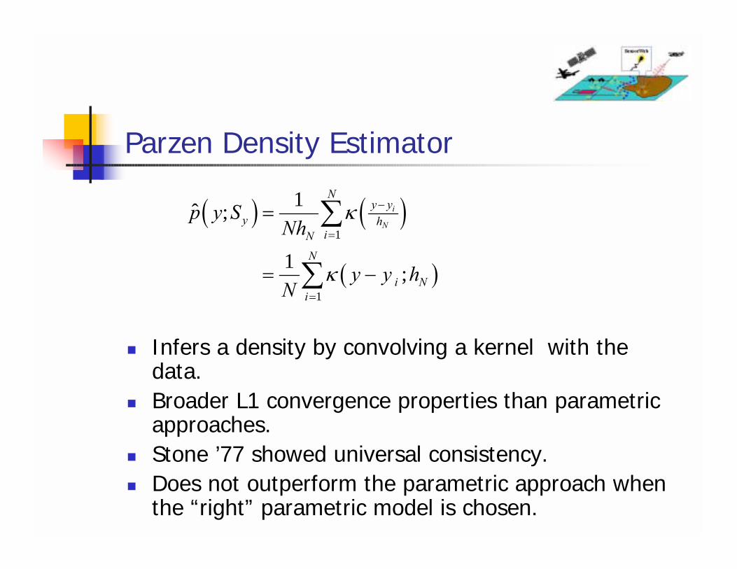
Parzen Density Estimator

! Infers a density by convolving a kernel with the data.

! Broader L1 convergence properties than parametric approaches.

! Stone ’77 showed universal consistency.! Does not outperform the parametric approach when

the “right” parametric model is chosen.

( ) ( )

( )

1

1

1ˆ ;

1 ;

i

N

Ny y

y hiN

N

i Ni

p y SNh

y y hN

κ

κ

−

=

=

=

= −

∑

∑

Exact Evaluation ofIntegral Criterion Gradient

Gradient of approximation can be computed exactly by evaluation of N functions at N sample locations.

( ) ( ) ( )( )

( ) ( )

( )( ) ( )

2

2

1

2

1

ˆ ˆ ˆlog2

1log ;2

1log ; ;2

Y

Y

y

Y

Y

y

Y

Y

y

u

N

i N ui

N

i N ui

VH p V p y p y dy

VV y y h p y dy

N

VV y g x h p y dy

N

κ

κ α

ΩΩ

Ω

ΩΩ

=Ω

ΩΩ

=Ω

= − −

= − − −

= − − −

∫

∑∫

∑∫

( )

( ) ( )( ) ( ) ( )

( ) ( ) ( )

1

ˆ ;

1 ;

;

; ; ;

YN

i ii

i r i a i j Nj i

r u z N

a N N z N

VH g x

N

f y y y hN

f y p y y h

y h y h y h

ε αα α

ε κ

κ

κ κ κ

Ω

=

≠

∂ ∂ = − ∂ ∂

= − −

= ∗

= ∗

∑

∑

Information Preserving TransformationsAdapt the mapping parameters, α, so as to maximize the information about the relevance parameter, θ.

( ),g α

feature extraction

θlabeled poses

back projection

PCA reconstruction

Complex temporal structure (Alex Ihler)

! Example from time-series modeling – pulsed laser data

! Learn a two dimensional statistic (which is a function of the past N samples) that has high mutual information with the next sample

! Low dimensionality does not necessarily equate to low complexity

Synthesis Examples

Gaussian assumption

1D Learned Statistic

2D Learned Statistic

Audio/Video fusion using MI

• Choose the mapping parameters such that the mutual information between the extracted features is maximized (i.e. project onto amaximally informative subspace.

• Why is this the “right” thing to do (or rather when)?

( , )i vg v α

( , )i ag a α

Independent Cause Model

A

B

C

V

U

( ) ( ) ( ) ( ) ( ) ( ), , , , , ,p A B C U V p A p B p C p U A B p V B C=

Induced dependency amongst causes

A

B

C

V

U

( ) ( ) ( ) ( ) ( ) ( )( ) ( ) ( ) ( )

, , , , , ,

, ,

p A B C U V p A p B p C p U A B

p U p A B U p C p

p C

C

V B

V B

=

=

Induced dependency amongst causes

A

B

C

V

U

( ) ( ) ( ) ( ) ( ) ( )( ) ( ) ( ) ( )( ) ( ) ( ) ( ), ,

, , , , , ,

, ,

p A B C U V p A p B p C p U A B p V B C

p

p V p

U p A B

B

U p C p V

C V p

B C

A p U A B

=

=

=

Joint observations increase complexity

A

B

C

V

U

( ) ( ) ( ) ( ) ( ) ( )( ) ( ) ( ) ( )( ) ( ) ( ) ( )( ) ( )

, , , , , ,

, ,

, ,

, , , ,

p A B C U V p A p B p C p U A B p V B C

p U p A B U p C p V B C

p V p B C V p A p U A B

p U V p A B C U V

=

=

=

=

Suppose a separation of U and V exists such that:

then…

Separating Functions

A

B

C

V

U

( ) ( ) ( ) ( ) ( )

( ) ( ) ( ) ( ) ( )

, ,

, ,

A B

B C

p U A B p A p B p U A p U B

p V B C p B p C p V B p V C

=

=

becomes

Bearing in mind that we still have the task of finding a separating function (or an approximate one).

Markov Property

A

B

C

VB

UA( ) ( ) ( ) ( )

( ) ( ) ( ) ( ), ,

A CB B

p A B C p A p C

p U

p B

p U B p VA B p V C

=

UB

VC

or

Markov Property

A

B

C

VB

UA( ) ( ) ( ) ( )

( ) ( ) ( ) ( )( ) ( ) ( )( ) ( ) ( ) ( )

, ,

A

B B B

B B C

A C

p A B C p A p B p C

p U A p U B p V B p V C

p A p C p

p U p B U p

U A

V

C

B

p V

=

=UB

VC

or

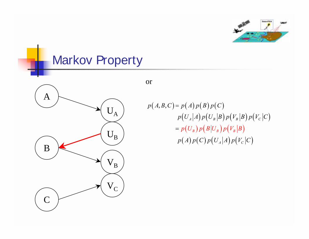
Markov Property

A

B

C

VB

UA( ) ( ) ( ) ( )

( ) ( ) ( ) ( )( ) ( ) ( )( ) ( ) ( ) ( )( ) ( ) ( )( ) ( ) ( ) ( )

, ,

A B B C

B B

B B B

B

A C

A C

p A B C p A p B p C

p U A p U B p V B p V C

p U p B U p V

p V p B V p U B

B

p A p C p U A p V C

p A p C p U A p V C

=

=

=

UB

VC

Audio/Video using MI

( , )i vg v α

( , )i ag a α

•By maximizing MI, we are summarizing the common information in the measurements, (i.e. which is related to their common cause).•From the information theory perspective, the joint of the feature variables is a proxy for the “observable” part of their common cause.

( ) ( )( ) ( )( )( ) ( )( ) ( )( )

, , , , ,

, , , , ,v u u

v u v

I g V g U I B g U

I g V g U I B g V

α α α

α α α

≤

≤

Maximally Informative SubspaceLearned Subspace

audio projection

video projection

Find a projection of both the video data and the audio data to a low-dimensional space such that MI is maximized.

Learning the Subspace

( ) ( )( ),

ˆ ˆ, arg max , , ,v a

v u v v a uI f V f Uα α

α α α α=

•The mapping parameters are chosen to maximize the mutual information in the low dimensional output space.

•Video localization and audio filter design are inferred as a function of the learned weights.

Video Localization of Single Speaker in the Presence of Motion Distractors

! Which pixels are “related” to the associated audio?

! Joint statistics of video and audio modalities are not well modeled by parametric forms.

! Slaney and Covell (NIPS ’00) demonstrate that canonical correlations (a second-order statistical measure) do not successfully detect audio/video synchrony using spectral representations.

! Classical sensor fusion approaches are formulated as joint Bayesian estimation problems, which is equivalent to MI in the non-parametric case.

Detecting (change) motion is not enough

•Red squares indicate regions with large pixel variance•Variance image of sequence at left•Magnitude of MAX MI video projection shown at center•Inspection of the learned video projection coefficients tells us which pixels are associated with the audio signal.

Representation: pixel vs. motion

•Similar result using an optic flow representation [Anandan ’89] of motion in the video•Fusion approach does not explicitly rely on how information is represented in data

Video Localization (more examples)

Audio Enhancement

•Left channel

•Right channel

•Wiener (left)

•Wiener (right)

•MI (left)

•MI (right)

In this experiment, regions of the video are selected for enhancement (e.g. face detector, manually).

Wiener Filter Comparison

5.6 dB5.7 dB10.5 dBSPG

(female voice)

9.2 dB8.9 dB10.43 dBSPG

(male voice)

Optical Flow-Periodogram

Representation

Pixel-Periodogram

RepresentationWiener filter

Acquiring correspondences

Acquiring correspondences

Peaks in mappingcoefficients

Acquiring correspondences

Peaks in mappingcoefficients

Extensions

! A basic algorithm has been developed! Need to incorporate multiple independent

causes (order estimation)! Temporal dependency of joint measurements! Testing on new data sources (e.g. audio,

seismic, etc.)

Exploiting array structure

! Two sensors observer mixture of three signals

! G( ) is unknown and may be nonlinear

! Use knowledge of the mixing structure to separate signals

A(t)

B(t)

C(t)

V(t)

U(t) ( ) ( ) ( )( ) ( ( )) ( )

U t A t B tV t G B t C t

= += +

A Variational Approach to Array Processing Accommodating

Sensor Location Uncertainties

Müjdat ÇetinStochastic Systems Group, M.I.T.

SensorWeb MURI Review Meeting June 18, 2001

The Source Localization Problem

! Find source location parameters based on data from multiple sensors

! Assumptions for a basic problem:! Unknown number of narrowband sources in near or far field! Omnidirectional sensors! Limited aperture size (" limited Rayleigh resolution) ! Sensor locations known only approximately

)()()()( ttt wsrAy +=

Variational Approach - Motivation

! View the problem as one of imaging a “source density” over the field of regard! Ill-posed inverse problem! Cast as an optimization problem and regularize by

favoring fields with concentrated densities! Can include optimization over sensor locations! Analogous to auto-focusing and point-enhanced imaging

in other array processing problems in which there are “phase defects” to be accommodated

Variational Formulation

! : non-quadratic function, e.g. norm! Preservation of strong features (source densities)! Preference of sparse source density field! Can resolve closely spaced radiating sources

! Sensor locations (boundedly) uncertain:! Self-calibration capability important

! Potential use in other domains:! SAR imaging with unknown motion of the objects in the scene! Robust Passive Sonar in the littoral

)()~()~,( 2

2ssrAyrs Ψ+−= λJ

)(⋅Ψ pl )1( ≤p

! Minimize the objective function:

ε<∞

)~,( rrd

Application in SAR Imaging

Ground truth ProposedConventional

# Superresolution Scatterer Localization (synthetic data)

Application in SAR Imaging

# Superresolution Scatterer Localization (real data)

Conventional Proposed

Application in SAR Imaging

# Region-Enhanced Imaging

Conventional Proposed

Moving Target Localization in SARConventional Proposed

# Scene contains 6 moving and 2 stationary strong point scatterers

Moving Target Localization in SAR

Detailed view

Velocity estimates

Summary and Extensions

! Proposed the development of a variational framework for passive source localization, robust to:! Limitations in data quality and quantity! Uncertainties in sensor locations

! Extensions:! Sensors: directional sensitivity, gain/phase uncertainties! Signals: structured broadband (e.g. harmonics),

unstructured or uncertain broadband! Medium: attenuating, dispersive, reverberant