further development of the sultan tool and scenarios … primes-tremove reference scenario was used...
TRANSCRIPT

EU Transport GHG: Routes to 2050 II Further development of the SULTAN tool and scenarios Contract 070307/2010/579469/SER/C2 for EU transport sector GHG reduction pathways to 2050
Restricted-Commercial Ref. AEA/ED56293/Task 6 Paper Draft – Issue No. 1 i
Further development of the SULTAN tool and scenarios for EU transport sector GHG reduction pathways to 2050
Nikolas Hill (AEA) Matthew Morris (AEA)
16 March 2012 Draft Final

Further development of the SULTAN tool and scenarios EU Transport GHG: Routes to 2050 II for EU transport sector GHG reduction pathways to 2050 Contract 070307/2010/579469/SER/C2
ii Ref. AEA/ED56293/Task 6 Paper Draft – Issue No. 1 Restricted-Commercial
Report Approved By: Signed:
Sujith Kollamthodi (AEA Practice Director - Transport)
Date:
<insert>
Report Approved By: Signed:
Sujith Kollamthodi (AEA Practice Director - Transport)
Date:
16 March 2012
Nikolas Hill (AEA) and Matthew Morris (AEA)
Further development of the SULTAN tool and scenarios for EU transport sector GHG reduction pathways to 2050
16 March 2012 Draft Final
Suggested citation: Nikolas Hill and Matthew Morris (2012) Further development of the SULTAN tool and scenarios for EU transport sector GHG reduction pathways to 2050. Task 6 paper produced as part of a contract between European Commission Directorate-General Climate Action and AEA Technology plc; see website www.eutransportghg2050.eu

EU Transport GHG: Routes to 2050 II Further development of the SULTAN tool and scenarios Contract 070307/2010/579469/SER/C2 for EU transport sector GHG reduction pathways to 2050
Restricted-Commercial Ref. AEA/ED56293/Task 6 Paper Draft – Issue No. 1 iii
Executive Summary
Objective: The purpose of this work was to develop the SULTAN Illustrative Scenarios Tool to further improve its usefulness for scoping possible impacts of policies on transport GHG emissions and to facilitate analysis to feed into other project tasks. This includes updating the baseline scenario to be consistent with recent Commission modelling and the development of additional policy scenarios and packages to feed into other project tasks.
Summary of Main Findings
SULTAN Development:
The SULTAN tool and its results viewer have been updated to provide a new baseline (business as usual) scenario, consistent with the latest Commission modelling, and with additional functionality to assist with scenario definition and impact analysis (including tables on biofuel use, energy security indicators, monetisation of emission impacts, etc).
Scenario Analysis:
In general the analysis illustrates the need for a balanced mix of well integrated policy actions to reduce the risk of failure to reach targets (maybe with an extra safety margin);
There are significant uncertainties around GHG savings from biofuel and electricity which pose a risk of very large gaps versus GHG targets if we become overly reliant on these options/do not act to mitigate/minimise these risk/uncertainties. Alternative options require a lead time for sufficient deployment by 2050, so need to be factored in early.
The exploration of sensitivities in demand showed the implication for higher demand was that additional/stronger actions may be needed to build contingency, e.g. in setting trajectories for new vehicle GHG standards, applying non-technical measures;
There is the potential for air quality, energy security and health co-benefits generating savings of up to €177B annually by 2050 versus business as usual (rising to up to €323B, including GHG savings). The greatest co-benefits per tonne GHG are achieved for actions that reduce vkm / shift to more efficient modes (particularly walking/cycling);
GHG emissions from vehicle production and disposal are significant (particularly for LDVs) and likely to grow in proportion to vehicle use emissions. Action should therefore be taken to minimise erosion of the benefits of GHG reduction policies. Providing such action is taken it is unlikely factoring in this aspect would alter the preferred/optimal pathway to total GHG reduction.
Introduction
The purpose of the task was to further develop and update the SULTAN Illustrative Scenario Tool developed in the previous project and carry out a range of additional scenario analysis. The ultimate objective of this task was to utilise the scenario analysis factoring findings from other project tasks to provide an effectively integrated/linked overall assessment. In discussion with the Commission at the project inception stage, the specific scope of the SULTAN and scenario development work to be covered as part of the Task 6 budget was agreed, as well as additional work to be carried out using some of the ad-hoc budget (Task 11). The following sub-tasks were carried out in accordance with the work agreed under Task 6 in order to meet the project objectives:

Further development of the SULTAN tool and scenarios EU Transport GHG: Routes to 2050 II for EU transport sector GHG reduction pathways to 2050 Contract 070307/2010/579469/SER/C2
iv Ref. AEA/ED56293/Task 6 Paper Draft – Issue No. 1 Restricted-Commercial
1) SULTAN Development:
a) Baseline update;
b) New functionality;
2) Scenario Analysis:
a) Simple scenarios;
b) Routes to 2050 sensitivity analysis;
c) Co-benefits and embedded GHG;
The following sections summarise the work carried out under each of these sub-task areas.
SULTAN Development
Update of baseline and original scenarios
Before any scenario analysis work could be completed it was necessary to update the SULTAN baseline dataset for the business as usual scenario (BAU-a) to be consistent with the most recent European Commission analysis. The previous baseline (SULTAN 2010 BAU-a) was developed based on the TREMOVE model version 2.7 baseline scenario, which excluded the effects of a range of elements including the impacts of the recent recession, as well as the impacts of a range of policies that have been implemented in the EU. In order to maintain consistency as far as possible with other Commission modelling work, the update of SULTAN carried out was based primarily on datasets provided directly by the Commission: the PRIMES-TREMOVE reference scenario was used as the primary source for the 2010-2050 projections (including activity, stock and energy carrier emission factors, with additionally supplementary data being sourced mainly from the TREMOVE v3.3.2 alternative baseline scenario (e.g. vehicle lifetimes, load factors, urban/rural/motorway split, NOX and PM emission factors, etc). Maritime shipping is currently not included in the PRIMES-TREMOVE or TREMOVE models, so updates to the SULTAN baseline were largely based on previous assumptions, plus estimates of the impact of the IMO’s energy efficiency design index (EEDI) targets announced in July 2011. The updated baseline was calibrated to be consistent with the PRIMES-TREMOVE reference scenario as closely as possible in terms of GHG emissions (first) and energy consumption (second) from 2010 to 2050. The resulting 2012 BAU-a scenario is compared to the old SULTAN 2010 BAU in the following Figure ES1.
Figure ES1: Comparison of the SULTAN business as usual scenarios from current and previous projects
0
200
400
600
800
1,000
1,200
1,400
1,600
1,800
2,000
2,200
2010 2015 2020 2025 2030 2035 2040 2045 2050
Co
mb
ine
d (life
cy
cle
) e
mis
sio
ns
, M
tCO
2e
Total Combined (life cycle) GHG emissions, BAU-a
FreightRail
MaritimeShipping
InlandShipping
HeavyTruck
MedTruck
Van
WalkCycle
Motorcycle
PassengerRail
IntlAviation
EUAviation
Bus
Car
Total WP Targets
SULTAN 2010 BAU
Notes: The ‘Total WP Targets’ figure indicated includes both the goal of reducing maritime emissions by 40%
by 2050, as well as the targets for the rest of transport in 2030 and 2050. The error bars on these points represent the range of values for these targets that were indicated in the 2050 Roadmap.

EU Transport GHG: Routes to 2050 II Further development of the SULTAN tool and scenarios Contract 070307/2010/579469/SER/C2 for EU transport sector GHG reduction pathways to 2050
Restricted-Commercial Ref. AEA/ED56293/Task 6 Paper Draft – Issue No. 1 v
The primary differences between the SULTAN 2012 and SULTAN 2010 baselines illustrated in Figure ES1 can be summarised as follows:
a) A lower 2010 starting point, reflecting the impacts of the recession (not included in the previous Commission modelling baseline);
b) Inclusion of 2020 regulatory CO2 targets for new cars (95 gCO2/km) and vans (147 gCO2/km) - only the 2015/17 targets were included in the baseline previously;
c) Significant activity modal shifts in passenger and freight transport and a 13% reduction in non-shipping tonne-km by 2050 (versus the previous baseline).
d) Maritime shipping GHG emissions now factor in the IMO’s new Energy Efficiency Design Index (EEDI) targets for new vessel efficiency (balancing demand growth);
e) Aviation activity and energy consumption is lower as this is now scaled to international bunkers, rather than full flight distance to/from EU countries (previously);
f) A reduction in the average road vehicle lifetimes used in the modelling, particularly for commercial vehicles where previously they were quite high vs European statistics.
New Functionality
In addition to the updating of the SULTAN baseline dataset, there were a number of other additional elements that have been developed in terms of new functionality for SULTAN, including improvements to both the assistance provided in the SULTAN Tool for scenario creation, and additional tables and charts in the SULTAN Results Viewer (e.g. monetised costs of GHG/NOx/PM emissions, information on biofuels and new energy security results).
Scenario Development and Analysis
New simple scenarios
As part of the specification and agreement of the scenario analysis with the commission the following simple scenarios were developed to explore key sensitivities, to complement the existing suite of 13 simple scenarios (plus BAU) developed under the previous project. These were as follows, with Figure ES2 providing a summary of the results from the analysis:
i. Scenario BAU-b: A low demand growth scenario (stabilisation post-2030);
ii. Scenario BAU-c: A high demand growth scenario;
iii. Scenario BAU-d: Alternative energy carrier GHG intensity trajectories in kgCO2e/MJ;
iv. Scenario 14-a: Additional fleet-wide GHG reduction measures for maritime shipping.
Figure ES2: Comparisons of the overall timeseries trajectories of GHG emissions for the different simple scenarios developed under Task 6 of the project
0
200
400
600
800
1,000
1,200
1,400
1,600
1,800
2010 2015 2020 2025 2030 2035 2040 2045 2050
Co
mb
ine
d (life
cycle
) e
mis
sio
ns, M
tCO
2e
Total Combined (life cycle) GHG emissions (Sum All)
BAU-a: Baseline
BAU-b: Low Demand
BAU-c: High Demand
BAU-d: High Energy Carrier GHG
14-a: Addit'l Maritime Ef f iciency
60% Reduction
80% Reduction
95% Reduction

Further development of the SULTAN tool and scenarios EU Transport GHG: Routes to 2050 II for EU transport sector GHG reduction pathways to 2050 Contract 070307/2010/579469/SER/C2
vi Ref. AEA/ED56293/Task 6 Paper Draft – Issue No. 1 Restricted-Commercial
The Figure shows that the alternative demand growth scenarios result in a -15% (~200MtCO2e) and +13% (~175MtCO2e) change in GHG emissions by 2050 respectively for low (BAU-b) and high (BAU-c) demand versus the base case (BAU-a). The alternative (pessimistic) assumptions on the future trajectories of energy carrier GHG intensity (BAU-d) lead to an increase of 10% (~125MtCO2e) in lifecycle GHG emissions by 2050 versus the base case. The most significant component of this increase is due to pessimistic assumptions on biofuel savings (in line with the no-action ILUC case from draft Commission impact assessment analysis available in the public domain). In possible alternative scenarios where more significant proportions of transport’s energy demand is met with electricity or hydrogen, the alternative assumptions for these energy carriers would be expected to have a greater effect. Additional maritime fleet efficiency measures (scenario 14-a) may be able to reduce lifecycle GHG emissions by 4% (~60MtCO2e) by 2050.
Central ‘Routes to 2050’ scenarios
As part of the project’s central scenario analysis a series of 5 core scenario packages/sensitivities were agreed with the Commission to explore key risks and uncertainties identified in other project tasks (i.e. Task 3, 4 and 5) in relation to meeting the EU’s overall target for GHG reduction by 2050 in the transport sector. A central Core GHG Reduction Scenario (R1) was developed to for the basis for the sensitivity analyses carried out for Task 6, as well as that carried out for Task 7 and the Task 11 ad-hoc analysis. This core scenario was developed according to the following general principals: 1) It was designed to achieve White Paper’s 60% GHG reduction target (on 1990 levels) for
transport excluding maritime shipping by 2050, and goal of 40% reduction in maritime shipping GHG (on 2005 levels) (R1-a = lifecycle GHG basis; R1-b = direct GHG basis);
2) Lower conventional fuel prices were used versus the baseline (BAU-a) scenario, consistent with the White Paper’s Impact Assessment Global Decarbonisation Scenario (provided by the Commission). A degree of rebound (in activity and increased vehicle energy consumption) resulting from these lower prices was factored into the calculations;
3) 2050 targets were assumed to be achieved through predominantly technical measures, plus additional measures broadly consistent with other White Paper Goals (e.g. internalising of external costs, additional shift of road freight transport to rail/IWW);
The methodology employed in carrying out the analysis was to take the core R1-a scenario as a basis and explore sensitivities in relation to this scenario:
a) Energy Carrier Sensitivities: The potential impacts of key energy carrier / technology risks and uncertainties identified in Task 5 were explored with scenarios R2 and R3 - potential impacts of low biofuel GHG savings and low biofuel AND low electricity GHG savings, respectively;
b) Demand Sensitivities: The potential impacts of variances in the growth of activity demand identified in Task 4 were explored with scenarios R4 and R5 (low and high demand scenarios respectively);
For the analysis a two-stage process was utilised for exploring potential implications:
(1) First amend the R1-a scenario assumptions for the area being explored to discover the resulting gap to reach the 2050 GHG emission targets;
(2) Re-adjust the scenario to again meet 2050 GHG targets by adding/strengthening or removing/relaxing GHG mitigation options as appropriate.
General Results
The following Figure ES3 provides a comparison of the different Routs to 2050 scenarios before adjustment has been made to the trajectories to bring them back to the 2050 targets.

EU Transport GHG: Routes to 2050 II Further development of the SULTAN tool and scenarios Contract 070307/2010/579469/SER/C2 for EU transport sector GHG reduction pathways to 2050
Restricted-Commercial Ref. AEA/ED56293/Task 6 Paper Draft – Issue No. 1 vii
Figure ES3: Comparisons of the overall timeseries trajectories of GHG emissions for the different Routes to 2050 sensitivity scenarios developed under Task 6 of the project (unadjusted*)
0
200
400
600
800
1,000
1,200
1,400
1,600
1,800
2010 2015 2020 2025 2030 2035 2040 2045 2050
Co
mb
ine
d (life
cycle
) e
mis
sio
ns, M
tCO
2e
Total Combined (life cycle) GHG emissions (Sum All)
BAU-a: Baseline
R1-a: Core GHG Reduction
R2-a: Low Biofuel Savings
R3-a: Low Bio+Elec Savings
R4-a: Low Demand
R5-a: High Demand
60% Reduction
80% Reduction
95% Reduction
Notes: * The ‘a’ and ‘c’ variants for scenarios R2-R5 have not been adjusted back in line with the 2050 GHG
reduction targets. The ‘b’ and ‘d’ variants have had their GHG emission trajectories adjusted back to the
2050 reduction targets by adding/strengthening or removing/relaxing GHG reduction measures.
The analysis shows that under the pessimistic biofuel savings assumptions (R2-a) there is a very substantial gap opened compared to the White Paper Target – a 43% increase in GHG (~230 MtCO2e), which further widens to 54% (~300 MtCO2e) if electricity GHG savings are also low (R3-a scenario). To close this latter gap in the second stage of the scenario analysis it was necessary to apply essentially all identified mitigation options to their maximum levels (as defined in the previous project). This results in very significant increases in technical efficiency, operational efficiency, and the application of measures to shift and ultimately reduce net transport activity further versus the core scenario (R1-a). The corresponding reduction in GHG emissions needed to bring them back to the 2050 targets is also significantly greater in some transport modes than for others (Figure ES4).
Figure ES4: Comparison of differences in annual lifecycle GHG emissions and demand for different Routes to 2050 scenarios relative to the core reduction scenario (R1a) for 2050
Unadjusted Scenarios Scenarios adjusted back to 2050 targets
-150
-100
-50
0
50
100
150
200
250
300
350
R1-a
: Core
GH
G R
eductio
n
R2-a
: Low
Bio
fuel S
avin
gs
R3-a
: Low
Bio
+E
lec S
avin
gs
R4-a
: Low
Dem
and
R5-a
: Hig
h D
em
and
Co
mb
ine
d (life
cycle
) e
mis
sio
ns, M
tCO
2e
(d
iffe
ren
ce
fro
m
R1
-a)
Total Combined (life cycle) GHG emissions, 2050FreightRail
MaritimeShipping
InlandShipping
HeavyTruck
MedTruck
Van
WalkCycle
Motorcycle
PassengerRail
IntlAviation
EUAviation
Bus
Car
-50
-40
-30
-20
-10
0
10
20
30
40
50
R1-a
: C
ore
GH
G R
eduction
R2-b
: Low
Bio
fuel S
avin
gs
R3-b
: Low
Bio
+E
lec S
avin
gs
R4-b
: Low
Dem
and
R5-b
: H
igh D
em
and
Co
mb
ine
d (life
cycle
) e
mis
sio
ns, M
tCO
2e
(d
iffe
ren
ce
fro
m
R1
-a)
Total Combined (life cycle) GHG emissions, 2050FreightRail
MaritimeShipping
InlandShipping
HeavyTruck
MedTruck
Van
WalkCycle
Motorcycle
PassengerRail
IntlAviation
EUAviation
Bus
Car
The corresponding variance to the 2050 GHG target for the low/demand scenarios are lower at -15%/+11% (-80/+60 MtCO2e) respectively, requiring fewer (but still significant) changes to the application of GHG mitigation measure in order to re-adjust back to target. For the low demand scenario (R4-b) the gap to 2050 GHG targets could be closed mainly through relaxed harmonisation of fuel taxes (air/ship demand increase, efficiency decrease), and

Further development of the SULTAN tool and scenarios EU Transport GHG: Routes to 2050 II for EU transport sector GHG reduction pathways to 2050 Contract 070307/2010/579469/SER/C2
viii Ref. AEA/ED56293/Task 6 Paper Draft – Issue No. 1 Restricted-Commercial
small reductions in biofuel % deployment. Conversely for the high demand scenario (R5-b) the gap to 2050 GHG targets may be closed through the application of a range of non-technical measures (e.g. eco-driving, speed reduction, spatial planning, etc). In terms of the levels of biofuel use, Figure ES5 illustrates that where additional action is taken to reduce GHG emissions, there may be very significant reductions in the volumes of biofuels needed to meet 2050 targets. For example, as applied in scenario R2 (and R3 to an even greater degree) this is a result of a combination of:
Vehicle efficiency improvements;
Substantial further shift to fully electrified powertrains (BEV, FCEV) in road transport;
Modal shift and activity reduction;
Reduced % deployment of biofuel (R2-d) with higher average GHG savings;
Figure ES5: Biofuel use in different Routes to 2050 scenarios in comparison to the baseline (BAU-a) and core reduction scenario (R1a)*
0
500
1,000
1,500
2,000
2,500
3,000
3,500
4,000
4,500
2010 2015 2020 2025 2030 2035 2040 2045 2050
PJ
Total energy supplied from biofuels by energy carrier (Sum All), BAU-a
LNG
Marine Fuels
Kerosene
CNG
LPG
Hydrogen
Electricity
Diesel
Gasoline
BAU-a total
0
500
1,000
1,500
2,000
2,500
3,000
3,500
4,000
4,500
2010 2015 2020 2025 2030 2035 2040 2045 2050
PJ
Total energy supplied from biofuels by energy carrier (Sum All), R1-a
LNG
Marine Fuels
Kerosene
CNG
LPG
Hydrogen
Electricity
Diesel
Gasoline
BAU-a total
BAU-a: Baseline Scenario R1-a: Core GHG Reduction Scenario
0
500
1,000
1,500
2,000
2,500
3,000
3,500
4,000
4,500
2010 2015 2020 2025 2030 2035 2040 2045 2050
PJ
Total energy supplied from biofuels by energy carrier (Sum All), R2-b
LNG
Marine Fuels
Kerosene
CNG
LPG
Hydrogen
Electricity
Diesel
Gasoline
BAU-a total
0
500
1,000
1,500
2,000
2,500
3,000
3,500
4,000
4,500
2010 2015 2020 2025 2030 2035 2040 2045 2050
PJ
Total energy supplied from biofuels by energy carrier (Sum All), R2-d
LNG
Marine Fuels
Kerosene
CNG
LPG
Hydrogen
Electricity
Diesel
Gasoline
BAU-a total
R2-b: Low Biofuel Savings R2-d: Low Biofuel Savings (Alt.)
Co-benefits and Embedded GHG Emissions
The analysis of the potential reduction of both direct and indirect air quality pollutant emissions from different scenarios showed substantial monetised benefits could be accrued. These benefits were estimated to be in the order of €45billion per annum versus the baseline for the core GHG reduction scenario (R1-a) by 2050. Further benefits are achieved from the energy carrier sensitivity scenarios (R2-R3), mainly due to reductions in overall demand/energy consumption needed to achieve 2050 GHG targets. The majority of air quality pollutant emissions are due to aviation and shipping by 2050 in all scenarios. In terms of energy security, the following Figure ES6 provides a summary of the likely implications for different scenarios using the methodology developed under Task 1 of the project. The charts show that there are anticipated to be significant energy security benefits resulting from action taken to meet 2050 GHG targets versus business as usual. The significantly increased benefits for R2-b and R3-b illustrated in the figure are mainly due to a reduction in overall energy consumption, which provides the highest energy security benefits.

EU Transport GHG: Routes to 2050 II Further development of the SULTAN tool and scenarios Contract 070307/2010/579469/SER/C2 for EU transport sector GHG reduction pathways to 2050
Restricted-Commercial Ref. AEA/ED56293/Task 6 Paper Draft – Issue No. 1 ix
Figure ES6: Comparison of the estimated impacts on energy security of the adjusted Routes to 2050 sensitivity scenarios with the baseline (BAU-a) scenario
0
20
40
60
80
100
Oil cost factor
Fleet readiness
Cost
Surplus capacity
Supply resilience
Resource concentration
BAU-a
2010 2030 2050
0
20
40
60
80
100Oil cost factor
Fleet readiness
Cost
Surplus capacity
Supply resilience
Resource concentration
R1-a: Core Reduction Scenario
2010 2030 2050
0
20
40
60
80
100Oil cost factor
Fleet readiness
Cost
Surplus capacity
Supply resilience
Resource concentration
R2-b: Low Biofuel Savings
2010 2030 2050
0
20
40
60
80
100Oil cost factor
Fleet readiness
Cost
Surplus capacity
Supply resilience
Resource concentration
R3-b: Low Bio+Elec Savings
2010 2030 2050
0
20
40
60
80
100Oil cost factor
Fleet readiness
Cost
Surplus capacity
Supply resilience
Resource concentration
R4-b: Low Demand
2010 2030 2050
0
20
40
60
80
100Oil cost factor
Fleet readiness
Cost
Surplus capacity
Supply resilience
Resource concentration
R5-b: High Demand
2010 2030 2050
Notes: The ‘b’ variants of scenarios R2-R5 have had their GHG emission trajectories adjusted back to the 2050
reduction targets by adding/strengthening or removing/relaxing GHG reduction measures.
In terms of the overall monetisation of co-benefits, Figure ES7 provides a summary of the potential overall benefits per annum by 2050 (versus BAU-a), which could be as high as €250 billion for R1-a or even reach €325 billion for R3-b. These are high-case estimates for those co-benefits that could be quantified for this project. However, additional noise, health and congestion co-benefits would likely further significantly add to these. The figure also provides an illustration of the importance of the benefits of walking and cycling which provide health co-benefits far higher than their relative contribution to GHG reduction, making policies that promote greater activity in this area particularly compelling.
Figure ES7: Summary of the total monetised co-benefits of the adjusted Routes to 2050 GHG reduction sensitivity scenarios versus the BAU scenario
0
50,000
100,000
150,000
200,000
250,000
300,000
350,000
Core 60% Red'n
Low Biofuel Savings
Low Bio+Elec Savings
Low Demand High Demand
R1-a R2-b R3-b R4-b R5-b
Mil
lio
n E
uro
s
Total Monetised Benefits of Scenario in 2050 (High GHG Cost) (High ES Cost)
Greenhouse Gases
Energy Security
Health (Walk/Cycle)
AQ Pollutants
Notes: Scenario ‘b’ variants of scenarios R2-R5 have had their GHG emission trajectories adjusted back to the
2050 reduction targets by adding/strengthening or removing/relaxing GHG reduction measures.

Further development of the SULTAN tool and scenarios EU Transport GHG: Routes to 2050 II for EU transport sector GHG reduction pathways to 2050 Contract 070307/2010/579469/SER/C2
x Ref. AEA/ED56293/Task 6 Paper Draft – Issue No. 1 Restricted-Commercial
According to analysis carried out under Task 21, GHG emissions from the production and disposal of new vehicles are anticipated to become an increasing component of a road transport vehicles lifetime emissions in the future. The results of the analysis show that their proportion could double, or in some cases triple for some modes in relation to total in-year transport energy consumption emissions. For example, for passenger cars this represents an increase from around 11% in 2010 to around 47% in 2050 for the R1-a scenario. This is mainly because improvements in the GHG intensity of vehicle production (with largest component being materials use) is not expected to reduce as fast as vehicle operational energy use GHG emissions. This is due to EU-level improvements being offset by (a) higher emissions from vehicle production/materials sourced from outside the EU; (b) higher GHG emissions from production for the most efficient technologies (e.g. electric, fuel cell vehicles), particularly in road transport. Nevertheless the study analysis has indicated that, although offset to a degree, the benefits of more efficient vehicle technologies in reducing emissions from energy consumption far outweigh possible disbenefits from higher production and disposal emissions. However, there are significant uncertainties in this aspect which mean that it will be important to take action minimise the likelihood of this component significantly eroding future benefits of alternative technologies in terms of GHG emissions from energy consumption. Figure ES8, provides a comparison of the different Task 6 sensitivity scenarios for passenger cars.
Figure ES8: Comparison of the total annual GHG emissions including vehicle production and disposal in 2050 for passenger cars for the different project Routes to 2050 scenarios
47.1%
37.2%33.2%
46.0%48.7%
59.2%
52.8%
43.6%
55.7%
0%
10%
20%
30%
40%
50%
60%
70%
80%
90%
100%
R1
a: C
ore
60
%
Re
d'n
R2
-a: L
ow
Bio
fue
l S
avin
gs
R3
-a: L
ow
B
io+
Ele
c S
avin
gs
R4
-a: L
ow
D
em
an
d
R5
-a: H
igh
D
em
an
d
R2
-b: L
ow
Bio
fue
l S
avin
gs
R3
-b: L
ow
B
io+
Ele
c S
avin
gs
R4
-b: L
ow
D
em
an
d
R5
-b: H
igh
D
em
an
d
GH
G p
rop
ort
ion
of
tota
l E
ne
rgy
LC
+V
eh
icle
LC
, %
Total annual GHG emissions VehicleLC, 2050 (Car)
Car Energy Consumption
Car Vehicle P&D/R
Notes: The ‘a’ variants for scenarios R2-R5 have not been adjusted back in line with the 2050 GHG reduction
targets. The ‘b’ variants have had their GHG emission trajectories adjusted back to the 2050 reduction targets by adding/strengthening or removing/relaxing GHG reduction measures.
1 Hill, N. et al (2012) The role of GHG emissions from infrastructure construction, vehicle manufacturing, and ELVs in overall transport sector
emissions. Task 2 paper produced as part of a contract between European Commission Directorate-General Climate Action and AEA Technology plc; see website www.eutransportghg2050.eu

EU Transport GHG: Routes to 2050 II Further development of the SULTAN tool and scenarios Contract 070307/2010/579469/SER/C2 for EU transport sector GHG reduction pathways to 2050
Restricted-Commercial Ref. AEA/ED56293/Task 6 Paper Draft – Issue No. 1 xi
Summary and Conclusions
SULTAN Development
The SULTAN tool and its results viewer have been updated to provide a new baseline (business as usual) scenario, consistent with the latest Commission modelling, and with additional functionality to assist with scenario definition and impact analysis (including tables on biofuel use, energy security indicators, monetisation of emission impacts, etc).
Scenario Analysis
General: – The analysis illustrates the need for a balanced mix of well integrated policy actions to
reduce the risk of failure to reach targets (maybe also with an extra safety margin);
Co-benefits (Task 1): – There is the potential for air quality, energy security and health co-benefits generating
savings of up to €177B annually by 2050 versus business as usual (rising to up to €323B, including GHG savings);
– The greatest co-benefits per tonne GHG are achieved for actions that reduce overall vkm / shift to more efficient modes (particularly for increasing walking and cycling);
Embedded GHG emissions (Task 2): – Vehicle production and disposal related GHG emissions are currently a significant
component of the vehicle lifecycle GHG footprint (particularly for LDVs) – accounting for an estimated 11% of all in-year transport GHG emissions. It is expected this proportion will increase significantly versus vehicle use GHG emissions in the future (potentially doubling on average, and more than tripling for some modes).
– It is therefore important to take action to ensure potential erosion of the GHG reduction benefits of policy actions is minimised as far as possible;
– However, it appears that this aspect is unlikely to alter the preferred/optimal pathway to total GHG reduction (e.g. there are still significant net GHG benefits for increasingly electrified road transport).
Knock-on consequences (Task 3): – GHG savings in all areas may not be as large as hoped for due to a variety of knock-
on consequences. – Therefore it may be desirable err on the side of caution in setting paths, for example
through the application of more stringent new road vehicle GHG standards – Stronger GHG standards would also provide additional air quality pollutant and
energy security co-benefits, plus reduce the biofuel volumes required to meet targets.
Decoupling of transport demand and GDP (Task 4): – One of the conclusions of Task 4 was that decoupling seems unlikely without a limited
number of specific policies (speed, pricing, land use), which could mean that the baseline assumptions of decoupling are over-optimistic.
– The exploration of sensitivities in demand showed the implication for higher demand was that additional/stronger actions may be needed to build contingency, e.g. in setting trajectories for new vehicle GHG standards, applying non-technical measures;
Risks & Uncertainties (Task 5): – Significant uncertainties around GHG savings from biofuel and electricity were
identified in Task 5 and assessed in the core sensitivity analysis. – These pose a risk very large gaps versus GHG targets if we become overly reliant on
these options/do not act to mitigate them. – Alternative options require a lead time for sufficient deployment by 2050, so need to
be factored in early.


EU Transport GHG: Routes to 2050 II Further development of the SULTAN tool and scenarios Contract 070307/2010/579469/SER/C2 for EU transport sector GHG reduction pathways to 2050
Restricted-Commercial Ref. AEA/ED56293/Task 6 Paper Draft – Issue No. 1 xiii
Table of Contents
Executive Summary ................................................................................................ iii
1 Introduction .................................................................................................... 20
1.1 Topic of this paper .............................................................................................20
1.2 The contribution of transport to GHG emissions ................................................20
1.3 Background to the project and its objectives .....................................................25
1.4 Background and purpose of the paper ..............................................................26
1.5 Structure of the paper .......................................................................................27
2 SULTAN Tool Development ........................................................................... 28
2.1 SULTAN Overview ............................................................................................28
2.1.1 Objective of the SULTAN tool............................................................................28
2.1.2 Data structure in the SULTAN tool ....................................................................29
2.1.3 Worksheets used ..............................................................................................30
2.1.4 Using the SULTAN tool .....................................................................................30
2.2 Updated SULTAN Functionality .........................................................................31
2.2.1 SULTAN Tool ....................................................................................................31
2.2.2 SULTAN Results Viewer ...................................................................................33
2.2.3 Using New Functionality in SULTAN .................................................................37
3 Scenario Development .................................................................................. 38
3.1 Updating the Baseline Scenario ........................................................................38
3.2 Updating the Original Scenarios ........................................................................44
3.3 New Simple Scenarios ......................................................................................45
3.3.1 Definition of the low demand growth scenario (BAU-b) .....................................46
3.3.2 Definition of the high demand growth scenario (BAU-c) ....................................48
3.3.3 Definition of the alternative energy carrier GHG intensity scenario (BAU-d) ......49
3.3.4 Definition of the maritime fleet efficiency measures scenario (14-a) ..................51
3.4 Routes to 2050 Scenarios .................................................................................52
3.4.1 Definition of the Core GHG Reduction Scenario (R1-a) .....................................53
3.4.2 Routes to 2050 Sensitivity Scenarios ................................................................58
4 Discussion of the Key Results from the Scenario Analysis ....................... 66
4.1 Introduction .......................................................................................................66
4.2 Alternative baselines and new simple scenarios ...............................................66
4.3 Routes to 2050 Scenarios .................................................................................67
4.3.1 General impacts on GHG emissions and other transport indicators ..................67

Further development of the SULTAN tool and scenarios EU Transport GHG: Routes to 2050 II for EU transport sector GHG reduction pathways to 2050 Contract 070307/2010/579469/SER/C2
xiv Ref. AEA/ED56293/Task 6 Paper Draft – Issue No. 1 Restricted-Commercial
4.3.2 Impacts on biofuel use ......................................................................................74
4.3.3 Impacts on GHG emissions from vehicle production and disposal ....................76
4.3.4 Impact on co-benefits: air pollutants and energy security ..................................79
5 Summary of Key Findings and Conclusions ............................................... 84
6 References ...................................................................................................... 86
Error! Reference source not found. ......................... Error! Bookmark not defined.
Error! Reference source not found. ........................... Error! Bookmark not defined.
Error! Reference source not found. ........................... Error! Bookmark not defined.

EU Transport GHG: Routes to 2050 II Further development of the SULTAN tool and scenarios Contract 070307/2010/579469/SER/C2 for EU transport sector GHG reduction pathways to 2050
Restricted-Commercial Ref. AEA/ED56293/Task 6 Paper Draft – Issue No. 1 xv
List of Tables
Table 2.1: Example of new Policy Scenario inputs for energy carrier emission factors, as viewed in the ‘Scenario_Editor’ sheet (shown for Maritime Shipping, R1-a Scenario) .......................................................................................................32
Table 2.2: Summary of inputs, assumptions and outputs for scenario development assistance calculations ..................................................................................33
Table 2.3: Summary of transport lifecycle GHG emissions reduction targets implemented in SULTAN ....................................................................................................37
Table 3.1: Comparison of average road vehicle lifetimes from the previous and new SULTAN versions ..........................................................................................42
Table 3.2: Summary list of the illustrative scenarios defined in SULTAN for the previous project ...........................................................................................................45
Table 3.3: EU projections in GDP, population and activity from 2010 to 2050 in the BAU-a scenario ......................................................................................................47
Table 3.4: Indexed projections of overall activity from 2010 to 2050 resulting from the low demand growth scenario (BAU-b) assumptions .............................................47
Table 3.5: Change in stock by mode in the low demand (BAU-b) scenario versus the baseline (BAU-a) scenario .............................................................................47
Table 3.6: Change in activity by mode in the low demand (BAU-b) scenario versus the baseline (BAU-a) scenario .............................................................................48
Table 3.7: Indexed projections of overall activity from 2010 to 2050 resulting from the high demand growth scenario (BAU-c) assumptions .....................................48
Table 3.8: Change in stock by mode in the high demand (BAU-c) scenario versus the baseline (BAU-a) scenario .............................................................................48
Table 3.9: Change in activity by mode in the high demand (BAU-c) scenario versus the baseline (BAU-a) scenario .............................................................................49
Table 3.10: Assumptions on average biofuel GHG savings versus conventional fuels utilised in different project scenarios ..............................................................50
Table 3.11: Alternate conventional liquid fuels scenario assumptions for BAU-d ..............50 Table 3.12: Assumptions on average electricity GHG emission factors and savings versus
1990 utilised in different project scenarios .....................................................51 Table 3.13: Assumptions on average hydrogen GHG emission factors utilised in different
project scenarios ...........................................................................................51 Table 3.14: Summary of estimates for potential reductions in CO2 emissions from maritime
shipping due to operational measures from IMO (2009) ................................52 Table 3.15: Summary of assumed impacts on maritime shipping fleet efficiency, overall
demand and load factors for scenario 14-a ....................................................52 Table 3.16: Summary of key assumptions in the Core GHG Reduction Scenario (R1-a)
meeting the White Paper main GHG reduction targets/objectives ..................54 Table 3.17: Summary of assumptions on improvements in overall new/fleet vehicle
efficiency for R1a (Non-powertrain technology % improvement in energy consumption versus BAU)* ............................................................................57
Table 3.18: External costs of climate change from IMPACT project (in €/tonne CO2), expressed as single values for a central estimate and lower and upper values ......................................................................................................................57
Table 3.19: External costs of NOx and PM used in defining illustrative scenarios ............57 Table 3.20: Summary of the key assumptions used in defining the sensitivity scenarios on
the implications for different road transport vehicle GHG trajectories .............62 Table 3.21: Summary of the key actions applied to the Routes to 2050 scenarios in order
to achieve GHG reduction targets for 2050 ....................................................64 Table 4.1: Potential impacts on energy security for different scenarios for 2050 .............82 Table 4.2: Assumptions on the cost factor for different impacts in 2050 .........................83

EU Transport GHG: Routes to 2050 II Further development of the SULTAN tool and scenarios Contract 070307/2010/579469/SER/C2 for EU transport sector GHG reduction pathways to 2050
Restricted-Commercial Ref. AEA/ED56293/Task 6 Paper Draft – Issue No. 1 xvi
List of Figures
Figure 1.1: EU27 greenhouse gas emissions by sector and mode of transport, 2009 ......20 Figure 1.2: Business as usual projected growth in transport’s lifecycle GHG emissions by
mode .............................................................................................................23 Figure 1.3: EU overall emissions trajectories against transport emissions (indexed) ........24 Figure 2.1: Role of the Illustrative Scenarios Tool in estimating the effect of future
transport policy ..............................................................................................28 Figure 2.2: Policy Scenario structure used in the SULTAN tool ........................................29 Figure 2.3: SULTAN worksheets showing the flow of information ....................................30 Figure 2.4: Schematic diagram of basic use of the SULTAN tool .....................................31 Figure 2.5: Example of new result showing biofuel energy supplied, and GHG emissions
abatement from biofuels split by energy carrier ..............................................33 Figure 2.6: Example of 5-year emissions budget chart for individual scenario .................34 Figure 2.7: Example of chart showing monetised costs of externalities by mode, and by
energy carrier for a single Policy Scenario .....................................................35 Figure 2.8: Example of radar diagram showing performance against six energy security
metrics for a single Policy Scenario in the years 2010, 2030 and 2050 ..........36 Figure 2.9: Example of chart showing overall performance against all six energy security
metrics for five Policy Scenarios for the period 2010 - 2050 ...........................36 Figure 2.10: Chart showing 2011 Transport White Paper (WP) targets for total GHG
emissions from the EU transport sector in 2030 and 2050, including permissible ranges ........................................................................................37
Figure 3.1: New vehicle technology penetration assumptions included in the new BAU scenario (BAU-a) ...........................................................................................39
Figure 3.2: Comparison of SULTAN business as usual scenarios from previous and current project................................................................................................40
Figure 3.3: Comparison of the SULTAN business as usual scenarios from current and previous projects ...........................................................................................41
Figure 3.4: Cumulative emissions profiles for SULTAN 2010 BAU and SULTAN 2012 BAU scenarios .......................................................................................................44
Figure 3.5: Comparison of passenger and freight demand for the alternative baselines and new simple scenarios ....................................................................................46
Figure 3.6: Comparison of the baseline (BAU-a) and Core GHG reduction scenario (R1-a) developed for the current project in the context of the Transport White Paper and 2050 Roadmap targets ...........................................................................53
Figure 3.7: New vehicle technology penetration assumptions included in the Core Scenario (R1-a) .............................................................................................56
Figure 3.8: New vehicle technology penetration assumptions in the R2-b/d Scenario ......60 Figure 3.9: New vehicle technology penetration assumptions in the R3-b/d Scenario ......61 Figure 4.1: Comparison of direct GHG emissions, lifecycle GHG emissions and energy
consumption for the alternative baselines and new simple scenarios ............67 Figure 4.2: Comparisons of the overall timeseries trajectories of GHG emissions for the
different Routes to 2050 sensitivity scenarios developed under Task 6 of the project (unadjusted*)......................................................................................68
Figure 4.3: Comparison of annual and cumulative lifecycle GHG emissions, energy consumption and demand for different scenarios relative to the core reduction scenario (R1a) for 2050 .................................................................................68
Figure 4.4: Comparison of the decomposition of impacts by scenario versus the baseline (BAU-a) .........................................................................................................70
Figure 4.5: Comparison of the temporal trends in overall direct GHG emissions, lifecycle GHG emissions, energy consumption and passenger / freight demand for

EU Transport GHG: Routes to 2050 II Further development of the SULTAN tool and scenarios Contract 070307/2010/579469/SER/C2 for EU transport sector GHG reduction pathways to 2050
Restricted-Commercial Ref. AEA/ED56293/Task 6 Paper Draft – Issue No. 1 xvii
different UNADJUSTED scenario ‘a’ variants*, relative to the BAU and core reduction scenario (R1-a) ..............................................................................71
Figure 4.6: New vehicle EFFICIENCY trajectories different Routes to 2050 scenarios in comparison to the baseline (BAU-a) and core reduction scenarios (R1a)* .....72
Figure 4.7: Comparison of the temporal trends in passenger / freight demand for different Routes to 2050 scenarios relative to the baseline (BAU-a) and core reduction scenario (R1a) ...............................................................................................73
Figure 4.8: Comparison of passenger and freight demand for different scenarios relative to the core reduction scenario (R1a) for 2050 ....................................................73
Figure 4.9: Biofuel use in different Routes to 2050 scenarios in comparison to the baseline (BAU-a) and core reduction scenario (R1a)* ..................................................75
Figure 4.10: Potential impacts on total annual lifecycle GHG emissions of factoring in emissions from the production and disposal of new vehicles for the core reduction scenario (R1-a) ..............................................................................76
Figure 4.11: Potential impacts on total lifecycle GHG emissions by 2050 of factoring in emissions from the production and disposal of new vehicles (all modes of transport) for different scenarios ....................................................................77
Figure 4.12: Potential 2050 impacts on total lifecycle GHG emissions of factoring in emissions from the production and disposal of new vehicles (all modes of transport) for different scenarios ....................................................................78
Figure 4.13: Comparison of the temporal trends in overall emissions of NOx and PM for different Routes to 2050 scenarios in comparison to the baseline (BAU-a) and core reduction scenario (R1a) ........................................................................80
Figure 4.14: Comparison of differences in annual NOx and PM emissions for different Routes to 2050 scenarios relative to the core reduction scenario (R1a) for 2050 ..............................................................................................................80
Figure 4.15: Potential impacts on emissions and external costs from air quality pollutants for different adjusted* scenarios in comparison to the baseline (BAU-a) and core scenario (R1-a) ......................................................................................81
Figure 4.16: Potential impacts on energy security for different scenarios* .........................82 Figure 4.17: Summary of the total monetised co-benefits of the adjusted Routes to 2050
GHG reduction sensitivity scenarios versus the BAU scenario ......................83

EU Transport GHG: Routes to 2050 II Further development of the SULTAN tool and scenarios Contract 070307/2010/579469/SER/C2 for EU transport sector GHG reduction pathways to 2050
Restricted-Commercial Ref. AEA/ED56293/Task 6 Paper Draft – Issue No. 1 xviii
Glossary2
BAU Business as usual, i.e. the projected baseline of a trend assuming that there are no interventions to influence the trend.
BEV Battery electric vehicle, also referred to as a pure electric vehicle, or simply a pure EV.
Biofuels A range of liquid and gaseous fuels that can be used in transport, which are produced from biomass. These can be blended with conventional fossil fuels or potentially used instead of such fuels.
Biogas A gaseous biofuel predominantly containing methane which can be used with or instead of conventional natural gas. Biogas used in transport is also referred to as biomethane to distinguish it from lower grade/unpurified biogas (e.g. from landfill) containing high proportions of CO2.
Biomethane Biomethane is the term often used to refer to/distinguish biogas used in transport from lower grade/unpurified biogas (e.g. from landfill) used for heat or electricity generation. Biomethane is typically purified from regular biogas to remove most of the CO2.
CNG Compressed Natural Gas. Natural gas can be compressed for use as a transport fuel (typically at 200bar pressure).
CO2 Carbon dioxide, the principal GHG emitted by transport.
CO2e Carbon dioxide equivalent. There are a range of GHGs whose relative strength is compared in terms of their equivalent impact to one tonne of CO2. When the total of a range of GHGs is presented, this is done in terms of CO2 equivalent or CO2e.
DG TREN European Commission’s Directorate-General on Transport and Energy. This DG was split in 2009 into DG Mobility and Transport (DG MOVE) and DG Energy.
Diesel The most common fossil fuel, which is used in various forms in a range of transport vehicles, e.g. heavy duty road vehicles, inland waterway and maritime vessels, as well as some trains.
EEA European Environment Agency.
EV Electric vehicle. A vehicle powered solely by electricity stored in on-board batteries, which are charged from the electricity grid.
FCEV Fuel cell electric vehicle. A vehicle powered by a fuel cell, which uses hydrogen as an energy carrier.
GHGs Greenhouse gases. Pollutant emissions from transport and other sources, which contribute to the greenhouse gas effect and climate change. GHG emissions from transport are largely CO2.
HEV Hybrid electric vehicle. A vehicle powered by both a conventional engine and an electric battery, which is charged when the engine is used.
ICE Internal combustion engine, as used in conventional vehicles powered by petrol, diesel, LPG and CNG.
Kerosene The principal fossil fuel used by aviation, also referred to as jet fuel or aviation turbine fuel in this context.
2 Terms highlighted in bold have a separate entry.

EU Transport GHG: Routes to 2050 II Further development of the SULTAN tool and scenarios Contract 070307/2010/579469/SER/C2 for EU transport sector GHG reduction pathways to 2050
Restricted-Commercial Ref. AEA/ED56293/Task 6 Paper Draft – Issue No. 1 xix
Lifecycle emissions
In relation to fuels, these are the total emissions generated in all of the various stages of the lifecycle of the fuel, including extraction, production, distribution and combustion. Also known as WTW emissions when limited specifically to the energy carrier/fuel.
LNG Liquefied Natural Gas. Natural gas can be liquefied for use as a transport fuel.
LPG Liquefied Petroleum Gas. A gaseous fuel, which is used in liquefied form as a transport fuel.
MtCO2e Million tonnes of CO2e.
Natural gas A gaseous fossil fuel, largely consisting of methane, which is used at low levels as a transport fuel in the EU.
NGV Natural Gas Vehicle. Vehicles using natural gas as a fuel, including in its compressed and liquefied forms.
NOx Oxides of nitrogen. These emissions are one of the principal pollutants generated from the burning of fossil and biofuels in transport vehicles.
Options These deliver GHG emissions reductions in transport and can be technical or non-technical.
Petrol Also known as gasoline and motor spirit. The principal fossil fuel used in light duty transport vehicles, such as cars and vans. This fuel is similar to aviation spirit also used in some light aircraft in civil aviation.
PHEV Plug-in hybrid electric vehicle, also known as extended range electric vehicle (ER-EV). Vehicles that are powered by both a conventional engine and an electric battery, which can be charged from the electricity grid. The battery is larger than that in an HEV, but smaller than that in an EV.
PM Particulate matter. These emissions are one of the principal pollutants generated from the burning of fossil and biofuels in transport vehicles.
Policy instrument
These may be implemented to promote the application of the options for reducing transport’s GHG emissions.
TTW emissions Tank to wheel emissions, also referred to as direct or tailpipe emissions. The emissions generated from the use of the fuel in the vehicle, i.e. in its combustion stage.
WTT emissions Well to tank emissions, also referred to as fuel cycle emissions. The total emissions generated in the various stages of the lifecycle of the fuel prior to combustion, i.e. from extraction, production and distribution.
WTW emissions Well to wheel emissions. Also known as lifecycle emissions when limited specifically to the energy carrier/fuel.

Further development of the SULTAN tool and scenarios EU Transport GHG: Routes to 2050 II for EU transport sector GHG reduction pathways to 2050 Contract 070307/2010/579469/SER/C2
20 Ref. AEA/ED56293/Task 6 Paper Draft – Issue No. 1 Restricted-Commercial
1 Introduction
1.1 Topic of this paper
This paper is one of a series of reports drafted under the EU Transport GHG: Routes to 2050 II project. These papers provide the results from each of the primary eight tasks from the project and will form the basis for chapter in the final report. This paper focuses on providing a summary of the work carried out for Task 6 of the project in further developing and updating the SULTAN Illustrative Scenario Tool developed in the previous project, and also the additional scenario analysis carried out for this new project.
1.2 The contribution of transport to GHG emissions
Transport is responsible for around a quarter of EU greenhouse gas emissions making it the second biggest greenhouse gas emitting sector after energy (see Figure 1.1). Road transport accounts for more than two-thirds of EU transport-related greenhouse gas emissions and over one-fifth of the EU's total emissions of carbon dioxide (CO2), the main greenhouse gas. However, there are also significant emissions from the aviation and maritime sectors and these sectors are experiencing the fastest growth in emissions, meaning that policies to reduce greenhouse gas emissions are required for a range of transport modes3.
Figure 1.1: EU27 greenhouse gas emissions by sector and mode of transport, 2009
10.8%
28.8%
6.5%
9.1%
3.5%
11.3%
5.1%
17.9%
0.4%
3.2%
0.4%
2.7%
0.2%
0.2%
Transport, 24.2%
Manufacturing and Construction Energy Industrial Processes
Residential Commercial Agricultrural
Other Road transport Domestic navigation
International maritime Domestic aviation International aviation
Rail transport Other transport
2009
Source: EEA (2012)
4
Notes: International aviation and maritime shipping only include emissions from bunker fuels
While greenhouse gas emissions from other sectors are generally falling, decreasing 24% between 1990 and 2009, those from transport have increased by 29% in the same period. This increase has happened despite improved vehicle efficiency because the amount of personal and freight transport has increased. The exception for this general upward trend in
3 EC DG Climate Action (2010): http://ec.europa.eu/clima/policies/transport/index_en.htm
4 Based on historic data from the EEA’s GHG data viewer, downloaded from EEA’s website 10/02/12: http://www.eea.europa.eu/data-and-
maps/data/data-viewers/greenhouse-gases-viewer

EU Transport GHG: Routes to 2050 II Further development of the SULTAN tool and scenarios Contract 070307/2010/579469/SER/C2 for EU transport sector GHG reduction pathways to 2050
Restricted-Commercial Ref. AEA/ED56293/Task 6 Paper Draft – Issue No. 1 21
emissions is the 5% decrease in overall transport emissions between 2007 (where they peaked) and 2009. This decrease is generally viewed as being primarily a result of the impacts of the global recession, and indications are that emissions began to rise again in 2010 as the European economy recovered somewhat. The European Commission (EC) has over the past year embarked on a number of programmes as part of the Europe 2020 Strategy, including the launch of Roadmap for moving to a competitive low carbon economy in 20505 (EC, 2011a – further referred as 2050 Roadmap) and Roadmap to a Single European Transport Area – Towards a competitive and resource efficient transport system (EC 2011b – further referred as Transport White Paper) – both published in March 2011.
The 2050 Roadmap is a strategy that seeks to define the most cost-effective ways to reduce
GHG emissions based on the outcome from modelling to meet the long-term target of reducing overall emissions by 80% domestically. The Roadmap considers the pathways for each of the sectors, identifying the magnitude of reductions required in each sector in 2030 and 2050 (shown as ranges) in a variety of scenarios ranging from under global co-operation on climate action to fragmented action. For the transport sector (which includes CO2 from aviation but excludes CO2 from marine shipping), the targets for 2030 are between +20% and -9%, and the 2050 targets are -54% to -67%. The Roadmap anticipates that the transport sector targets could be achieved through a combination of fuel efficiency, electrification and consideration of transport prices. These are explored further in the White Paper on Transport on the basis of the Effective Technology scenario (with low fossil fuel prices) of the Roadmap which shows a -61% reduction for the transport sector. The Transport White Paper6 presents the European Commission’s vision for the future of the EU transport system and defines a policy agenda for the next decade to begin to move towards a 60% reduction in CO2 emissions and comparable reduction in oil dependency by 2050. As part of this it defines ten aspirational goals as indicators for policy action. These goals can be categorised as developing and deploying new and sustainable fuels and propulsion systems; optimising the performance of multimodal logistic chains, including by making greater use of more energy efficient modes; and increasing the efficiency of transport and of infrastructure use with information systems and market-based incentives. Key goals are presented below.
Box 1.1: Goals from the 2011 Transport White Paper
EC Transport White Paper Goals (2011)
Halve the use of ‘conventionally-fuelled’ cars in urban transport by 2030; phase them out in cities by 2050; achieve essentially CO2-free city logistics in major urban centres by 2030.
Low-carbon sustainable fuels in aviation to reach 40% by 2050; also by 2050 reduce EU CO2 emissions from maritime bunker fuels by 40% (if feasible 50%).
30% of road freight over 300 km should shift to other modes such as rail or waterborne transport by 2030, and more than 50% by 2050, facilitated by efficient and green freight corridors. To meet this goal will also require appropriate infrastructure to be developed.
By 2050, complete a European high-speed rail network. Triple the length of the existing high-speed rail network by 2030 and maintain a dense railway network in all Member States. By 2050 the majority of medium-distance passenger transport should go by rail.
A fully functional and EU-wide multimodal TEN-T ‘core network’ by 2030, with a high quality and capacity network by 2050 and a corresponding set of information services.
5 EC (2011a) A Roadmap for moving to a competitive low carbon economy in 2050, COM(2011) 112 final, European Commission. Brussels.
Available at: http://ec.europa.eu/clima/policies/roadmap/documentation_en.htm 6 EC (2011b) Roadmap to a Single European Transport Area – Towards a competitive and resource efficient transport system, COM(2011) 144
final, European Commission, Brussels. Available at: http://ec.europa.eu/transport/strategies/2011_white_paper_en.htm

Further development of the SULTAN tool and scenarios EU Transport GHG: Routes to 2050 II for EU transport sector GHG reduction pathways to 2050 Contract 070307/2010/579469/SER/C2
22 Ref. AEA/ED56293/Task 6 Paper Draft – Issue No. 1 Restricted-Commercial
EC Transport White Paper Goals (2011)
By 2050, connect all core network airports to the rail network, preferably high-speed; ensure that all core seaports are sufficiently connected to the rail freight and, where possible, inland waterway system.
Deployment of the modernised air traffic management infrastructure (SESAR) in Europe by 2020 and completion of the European Common Aviation Area. Deployment of equivalent land and waterborne transport management systems (ERTMS, ITS, SSN and LRIT, RIS). Deployment of the European Global Navigation Satellite System (Galileo).
By 2020, establish the framework for a European multimodal transport information, management and payment system.
By 2050, move close to zero fatalities in road transport. In line with this goal, the EU aims at halving road casualties by 2020. Make sure that the EU is a world leader in safety and security of transport in all modes of transport.
Move towards full application of “user pays” and “polluter pays” principles and private sector engagement to eliminate distortions, including harmful subsidies, generate revenues and ensure financing for future transport investments.
The Transport White Paper goals are underpinned by 40 concrete initiatives, and the various actions and measures introduced within the Paper will be elaborated on over this decade through the preparation of appropriate legislative proposals with key initiatives to be put in place. The actions aim to increase the competitiveness of transport while contributing to delivering the 60% reduction in GHG emissions from transport required by 2050, using the ten goal/targets as benchmarks. Both the 2050 Roadmap and Transport White Paper set the context within which this EU Transport GHG: Routes to 2050 II project has been undertaken, although this work was commissioned prior to their completion. The increasing political importance that is being attached to decarbonising transport reflects the fact that, of all the economy’s sectors, transport has made the least progress in terms of reducing its GHG emissions, despite significant potential at low cost. As mentioned earlier, since 1990, GHG emissions from transport, of which 98% are carbon dioxide (CO2), had the highest increase in percentage terms of all energy related sectors7 (even without non-CO2 impacts of aviation being included). Figure 1.2 shows the updated baseline based on PRIMES-TREMOVE, as implemented in SULTAN. This is consistent with the range of results from other models and tools, although many of these only project to 20308. The previous baseline based on TREMOVE (total combined GHG emissions, 2010) is also indicated in the figure (showing WTW/fuel lifecycle emissions). Whereas the 2010 baseline anticipated continued growth in the EU-27’s GHG emissions from transport, the updated baseline sees a decline in GHG emissions over the period to 2050. This is mainly due to a range of existing and planned policies being included in the new baseline, including the 2020 regulatory targets CO2 emissions for passenger cars and vans, the IMO Energy Efficiency Design Index (EEDI) based improvement targets for maritime shipping and estimated impacts of including aviation in the EU ETS. Another factor is that it also includes impacts of the recession on transport sector GHG emissions, which affects mainly the 2010 starting point but also has some roll-on effects. Even a decrease in the order projected in Figure 1.2 for the updated baseline would leave transport’s WTW (fuel lifecycle) GHG emissions 17% higher in 2050 than they were in 1990 (when the sector’s emissions were nearly 1,200 MtCO2e). This is a decline of 22% on 2010 GHG levels (which were around 32% above those in 1990).
7 DG TREN (2000) Energy and transport in figures 2008-2009
8 See Appendix 19 SULTAN: Development of an Illustrative Scenarios Tool for Assessing Potential Impacts of Measures on EU Transport GHG for
details of the assumptions used and approach taken in the SULTAN Illustrative Scenarios Tool to projecting business as usual GHG emissions; also see http://www.eutransportghg2050.eu

EU Transport GHG: Routes to 2050 II Further development of the SULTAN tool and scenarios Contract 070307/2010/579469/SER/C2 for EU transport sector GHG reduction pathways to 2050
Restricted-Commercial Ref. AEA/ED56293/Task 6 Paper Draft – Issue No. 1 23
Large increases in emissions between 2010 and 2050 are projected for aviation and maritime without additional policy instruments (by 42% and 22% respectively, even after recent policy developments). Under the previous baseline scenario, road freight volume was projected to increase significantly, however, due to significantly reduced levels of demand growth in the new PRIMES Reference Scenario (and some additional modal shift), it is now projected to have slightly decreased by 2050. Whilst GHG emissions from cars are still projected to contribute the most to the sector’s GHG emissions in absolute terms in 2050, their emissions are projected to have declined significantly from 2010 levels, due to the impacts of the 2020 regulatory CO2 targets.
Figure 1.2: Business as usual projected growth in transport’s lifecycle GHG emissions by mode
0
200
400
600
800
1,000
1,200
1,400
1,600
1,800
2,000
2,200
2010 2015 2020 2025 2030 2035 2040 2045 2050
Co
mb
ine
d (life
cy
cle
) e
mis
sio
ns
, M
tCO
2e
Total Combined (life cycle) GHG emissions, BAU-a
FreightRail
MaritimeShipping
InlandShipping
HeavyTruck
MedTruck
Van
WalkCycle
Motorcycle
PassengerRail
IntlAviation
EUAviation
Bus
Car
Total WP Targets
SULTAN 2010 BAU
Source: SULTAN Illustrative Scenarios Tool, updated for the EU Transport GHG: Routes to 2050 II project
Notes: Maritime shipping include estimates for the full emissions resulting from journeys to EU countries, rather than current international reporting which only include emissions from bunker fuels supplied at a country level (which are lower by around 18%). Previous SULTAN 2010 BAU included also international aviation on a similar basis. The new baseline has been developed to be consistent with the latest EC modelling reference scenarios and includes (a) the impact of the recession, (b) aviation based on bunkers, (c) includes additional policies and measures that were not in the previous baseline, including the 2020 Car CO2 regulatory targets, the new Energy Efficiency Design Index (EEDI) targets for maritime shipping, and the estimated impacts of including aviation in the EU ETS. The ‘Total WP Targets’ figure indicated includes both the goal of reducing maritime emissions by 40% by 2050, as well as the targets for the rest of transport in 2030 and 2050.
Despite the overall projected reduction in transport sector GHG emissions to 2050, this decline is not enough. If no action is taken to reduce these emissions, the EU will not meet the long-term GHG emission reduction targets that the European Council supports in 2030 and 2050. Figure 1.3 demonstrates that on current trends, transport emissions could reach levels around 20% of economy-wide 1990 GHG emissions by 20509 if unchecked. This would also
9 The emissions included in this figure – for both the economy-wide emissions and those of the transport sector – include emissions from
international aviation and maritime transport, in addition to emissions from “domestic” EU transport.

Further development of the SULTAN tool and scenarios EU Transport GHG: Routes to 2050 II for EU transport sector GHG reduction pathways to 2050 Contract 070307/2010/579469/SER/C2
24 Ref. AEA/ED56293/Task 6 Paper Draft – Issue No. 1 Restricted-Commercial
be equivalent to the budget total EU-wide GHG emissions for an 80% reduction target across all sectors. The figure also illustrates the 2050 Roadmap and White Paper targets for transport (54% to 67% reduction and 60% reduction in emissions compared to 1990 levels respectively for transport excluding maritime shipping, and the 40% GHG reduction goal for maritime transport from the White Paper). Whilst simplistic, in that it assumes linear reductions, the figure demonstrates that there is clearly a need for additional policy instruments to stimulate the take up of technical and non-technical options that could potentially reduce transport’s GHG emissions.
Figure 1.3: EU overall emissions trajectories against transport emissions (indexed)
0%
20%
40%
60%
80%
100%
120%
1990 2000 2010 2020 2030 2040 2050
EU
-27
GH
G e
mis
sio
ns
(1
99
0 =
10
0%
)
EU-27 transport BAU projection (SULTAN 2011)
EU-27 transport BAU projection (SULTAN 2010)
EU-27 transport
EU-27 all sectors
60 - 80%
80 - 95%
0%
5%
10%
15%
20%
25%
30%
35%
1990 2000 2010 2020 2030 2040 2050
EU
-27
GH
G e
mis
sio
ns
(1
99
0 =
10
0%
)
Transport BAU (SULTAN 2011)
Transport BAU (SULTAN 2010)
White Paper 2011 Target
2050 Roadmap (low transport)
2050 Roadmap (high transport)
EU-27 transport (historic)
2050 Roadmap: Transport -54 to -67% Reduction
Mainlyinclusion of additional
policies and measures, recession.
Source: EEA (2012)
10 and SULTAN Illustrative Scenarios Tool
11
10
Based on historic data from the EEA’s GHG data viewer, downloaded from EEA’s website 10/02/12: http://www.eea.europa.eu/data-and-maps/data/data-viewers/greenhouse-gases-viewer 11
Projections based on data from the SULTAN Illustrative Scenarios Tool (BAU-a scenario) and historic data from DG MOVE (2011) EU energy and transport in figures Statistical Pocketbook 2011 Luxembourg, Publications Office of the European Union, 2010.

EU Transport GHG: Routes to 2050 II Further development of the SULTAN tool and scenarios Contract 070307/2010/579469/SER/C2 for EU transport sector GHG reduction pathways to 2050
Restricted-Commercial Ref. AEA/ED56293/Task 6 Paper Draft – Issue No. 1 25
1.3 Background to the project and its objectives
EU Transport GHG: Routes to 2050 II is a 15-month project funded by the European Commission's DG Climate Action and started in January 2011. The context of the project is still the Commission's long-term objective for tackling climate change. The scope of the first project was very ambitious, and the outputs from the project were very detailed and have already proved to be of great value to the European Commission and to industry, governmental and NGO stakeholders. However, there were a number of topic areas where it was not possible within the time and resources available for the team to carry out completely comprehensive research and analysis. In particular, as the project evolved, both the team and the Commission Services became aware that there were a number of themes and topic areas that would benefit from further, more detailed research. This new project is a direct follow-on piece of analysis to the previous EU Transport GHG: Routes to 2050? project, building on the investigations and analysis carried out for that project and complementing other work carried out for the Transport White Paper. In particular, the outputs from this new project should be useful to the Commission in prioritising and developing the key future policy measures that will be critical in ensuring that GHG emissions from the transport sector can be reduced significantly in future years. Therefore, the key objectives of the EU Transport GHG: Routes to 2050 II have been defined as to build on the work carried out in the previous project to:
- Develop an enhanced understanding of the wider potential impacts of transport GHG reduction policies, as well as their possible significance in a critical path to GHG reductions to 2050.
- Further develop the SULTAN illustrative scenarios tool to enhance its usefulness as a policy scoping tool and carry out further scenario analysis in support of the new project;
- Use the new information in the evaluation of a series of alternative pathways to transport GHG reduction for 2050, in the context of the 54-67% reduction target for transport from the European Commission's Roadmap for moving to a competitive low carbon economy in 205012;
As before, given the timescales being considered, the project has taken a quantitative approach to the analysis where possible, and a qualitative approach where this has not been feasible. The project has been structured against a number tasks, which are as follows:
Task 1: Development of a better understanding of the scale of co-benefits associated with transport sector GHG reduction policies;
Task 2: The role of GHG emissions from infrastructure construction, vehicle manufacturing, and ELVs in overall transport sector emissions;
Task 3: Exploration of the knock-on consequences of relevant potential policies;
Task 4: Exploration of the potential for less transport-intensive paths to societal goals;
Task 5: Identification of the major risks/uncertainties associated with the achievability of the policies and measures considered in the illustrative scenarios;
Task 6: Further development of the SULTAN tool and illustrative scenarios;
Task 7: Exploration of the interaction between the policies that can be put in place prior to 2020 and those achievable later in the time period;
12
Communication from the Commission to the European Parliament, the Council, the European Economic and Social Committee and the Committee of the Regions, A Roadmap for moving to a competitive low carbon economy in 2050, COM(2011) 112 final. Available from DG Climate Actions website at: http://ec.europa.eu/clima/policies/roadmap/index_en.htm

Further development of the SULTAN tool and scenarios EU Transport GHG: Routes to 2050 II for EU transport sector GHG reduction pathways to 2050 Contract 070307/2010/579469/SER/C2
26 Ref. AEA/ED56293/Task 6 Paper Draft – Issue No. 1 Restricted-Commercial
Task 8: Development of a better understanding of the cost effectiveness of different policies and policy packages;
Task 9: Stakeholder engagement: organisation of technical level meetings for experts and stakeholders;
Task 10: Hosting the existing project website and its content;
Task 11: Ad-hoc work requests to cover work beyond that covered in the rest of the work plan.
As in the previous project, stakeholder engagement has been an important element of the project. The following meetings have been held:
A large stakeholder meeting was held in on 29th June 2011, at which this project was introduced to stakeholders, along with the presentation of interim results.
A series of four Technical Focus Group meetings. The first two were held on 4th May 2011and the second two were held on 28th November 2011.
A second large stakeholder meeting at which the draft final findings of the project were presented and discussed, was held on 23rd February 2012.
As part of the project a number of papers have been produced, all of which have been made available on the project’s website in draft and then final form, as have all of the presentations from the project’s meetings.
1.4 Background and purpose of the paper
The purpose of Task 6 was to further develop and update the SULTAN Illustrative Scenario Tool developed in the previous project and carry out a range of additional scenario analysis. The ultimate objective of this task was to utilise the scenario analysis factoring findings from other project tasks to provide an effectively integrated/linked overall assessment. There were a wide number of possibilities for the development of SULTAN, and it was only possible to develop a selection of these within the available resource for this work. In addition, there were many potential linkages with other project tasks – at the very least SULTAN and the policy scenarios were to be developed further and utilised for Task 7 (impacts of policies that could be implemented by 2020). In discussion with the Commission at the project inception stage, the specific scope of the SULTAN and scenario development work to be covered as part of the Task 6 budget was agreed, as well as additional work to be carried out using some of the ad-hoc budget (Task 11). The following sub-tasks were carried out in accordance with the work agreed under Task 6 in order to meet the project objectives:
1) SULTAN Development:
a) Baseline update;
b) New functionality;
2) Scenario Analysis:
a) Simple scenarios;
b) Routes to 2050 sensitivity analysis;
c) Co-benefits and embedded GHG;
d) [New road vehicle GHG emission standard trajectories (Task 11 Paper 2)].
The following report chapters summarise the work carried out under each of these sub-task areas, with the exception of the work on new road vehicle GHG emission standard trajectories, which is detailed separately in Task 11 Paper 2.

EU Transport GHG: Routes to 2050 II Further development of the SULTAN tool and scenarios Contract 070307/2010/579469/SER/C2 for EU transport sector GHG reduction pathways to 2050
Restricted-Commercial Ref. AEA/ED56293/Task 6 Paper Draft – Issue No. 1 27
1.5 Structure of the paper
Following this introduction this paper is structured according to the following further chapters:
Chapter 2 SULTAN Tool Development: This section provides a summary of the updates to the design, structure, content and functionality of the SULTAN tool.
Chapter 3 Scenario Development: This section provides an overview of the selection and definition of the new baseline and other scenarios explored using the SULTAN tool, including key assumptions and sources of information.
Chapter 4 Discussion of the Key Results from the Scenario Analysis: In this section there is a discussion of some of the key results from the various scenarios developed under Task 6.
Chapter 5 Summary of Key Findings and Conclusions: This section provides a final summary of the key findings from the analysis and the conclusions that may be drawn for the rest of the work.
Chapter 6 References
Error! Reference source not found.: The appendices provide additional detail on the assumptions used in the definition of the illustrative scenarios.

Further development of the SULTAN tool and scenarios EU Transport GHG: Routes to 2050 II for EU transport sector GHG reduction pathways to 2050 Contract 070307/2010/579469/SER/C2
28 Ref. AEA/ED56293/Task 6 Paper Draft – Issue No. 1 Restricted-Commercial
2 SULTAN Tool Development
The SULTAN (SUstainabLe TrANsport) Illustrative Scenario tool was developed as part of the original Routes to 2050 project to provide a quantitative framework for the project outputs. It was used to produce the “Routes to 2050” scenarios, exploring a range of possibilities for packages of policy options that could achieve the desired reduction in GHG emissions from the European transport system to 2050. The tool allowed the consequences of these scenarios to be explored in detail in terms of emissions from each mode, activity levels, and costs. In this project, the SULTAN tool has again been used to reflect the quantitative outputs of the various study papers, and to produce a further set of scenarios. In addition, the input data have been updated to reflect the latest European modelling outputs used by the Commission in other studies. The functionality of the tool has also been updated and extended, to reflect the extra topics covered in this study. This includes more explicit tracking of biofuels, calculations to estimate the co-benefits of policies (energy security, air quality pollutants) and the external costs of pollutant emissions, and functionality to explore emissions budgets. This section gives a brief overview of the SULTAN tool and describes the updated functionality.
2.1 SULTAN Overview
2.1.1 Objective of the SULTAN tool
The SULTAN tool is a calculation framework that allows users to quickly estimate the impacts of policy on the European transport system by building ‘Policy Scenarios’. Each Policy Scenario is a possible outcome that describes the evolution of the European transport system from 2010-2050. Users build Policy Scenarios by estimating the impacts of policy and other drivers on a variety of input parameters such as demand for transport, vehicle stock, and the types of vehicle powertrains that are used. The tool calculates the impacts of these scenarios on a range of outputs including GHG emissions, co-benefits, and costs. Figure 2.1 illustrates this process.
Figure 2.1: Role of the Illustrative Scenarios Tool in estimating the effect of future transport policy
Range of policy
options
Impacts (activity, efficiency etc.) estimated
Aggregated into Policy Scenarios
Illustrative Scenario Tool
Estimate of emissions and costs from the sector under the
The approach taken in designing the tool was as follows:
Scope: The tool covers all EU27 member states, for the years 2010 to 2050. All major modes of passenger and freight transport are included so that the vast majority of GHG emissions from the transport sector are captured. There are no inputs or results at the member-state level.
Simplicity: The tool has been designed to be as simple as possible whilst achieving the necessary level of accuracy. There is no modelling involved; the tool does not attempt to predict or optimise the outcomes by iteration. Instead, the tool acts as a simple calculator, producing results by direct calculation from the inputs supplied. The

EU Transport GHG: Routes to 2050 II Further development of the SULTAN tool and scenarios Contract 070307/2010/579469/SER/C2 for EU transport sector GHG reduction pathways to 2050
Restricted-Commercial Ref. AEA/ED56293/Task 6 Paper Draft – Issue No. 1 29
number of inputs, calculation and level of detail are all as low as possible whilst maintaining a reasonable degree of accuracy; complex and detailed calculations would be unlikely to significantly improve accuracy in any case, given the large range of uncertainty associated with making predictions out to 40 years in the future.
Transparency: The simplicity of calculations, along with the accessible format of the tool, is intended to make it as transparent as possible. The tool is based in Microsoft Excel, with the intention that stakeholders will quickly be able to view the inputs and calculations in a familiar format.
2.1.2 Data structure in the SULTAN tool
The input and output data in the SULTAN tool is divided into modes, powertrains and fuels, as illustrated in Figure 2.2.
Figure 2.2: Policy Scenario structure used in the SULTAN tool
Policy Scenario
One possible route to 2050 for European transport
Modes(7 passenger, 6 freight)
All major modes of transport covered
Powertrain technologies(up to 10)
Current and future options for vehicle drivetrains
Energy carriers / fuels (up to 7)
Each powertrain technology can use up to 3
Modes, powertrains and fuels are broadly defined as follows:
Modes perform different functions within the transport network. Different modes satisfy different types of passenger \ freight demand (e.g. high or low value goods) and \ or provide different range, speed or flexibility of transport.
Powertrains are (usually) broadly interchangeable technologies used to power vehicles within a mode. All vehicles in a mode fall into one of the powertrain categories within it. Each powertrain has different physical characteristics, e.g. cost, energy efficiency, fuels and load factor.
Fuels are energy carriers that supply energy to powertrains. Each powertrain can be potentially powered by up to three fuels, though only some powertrains are multi-fuel as implemented (e.g. plug-in hybrid electric vehicles). Each fuel has different emissions factors and costs per unit of energy supplied. Biofuels are not explicitly included as fuels in the tool; instead, they are implicitly accounted for by changing the emissions factors of conventional fuels.

Further development of the SULTAN tool and scenarios EU Transport GHG: Routes to 2050 II for EU transport sector GHG reduction pathways to 2050 Contract 070307/2010/579469/SER/C2
30 Ref. AEA/ED56293/Task 6 Paper Draft – Issue No. 1 Restricted-Commercial
2.1.3 Worksheets used
The SULTAN tool is divided into two Excel worksheets: the main tool itself, and a dedicated results viewing tool. In addition, each policy scenario has inputs stored in a separate database worksheet. When the tool is run, outputs are also written to a database worksheet. This relationship is shown in Figure 2.3.
Figure 2.3: SULTAN worksheets showing the flow of information
Policy
Scenario
database
SULTAN Tool
Results
database
SULTAN
Results
Viewer
The Policy Scenario database contains all the input data needed to run a Policy Scenario through the tool. Data are stored in a database format in an excel worksheet. Data for multiple Policy Scenarios can be stored in a single file. The input data can be viewed and edited directly, or edited using functionality within the SULTAN tool.
The SULTAN tool is the main file that is used to create, edit and run Policy Scenarios. It contains worksheets that allow the user to select Policy Scenarios, view and edit all of the inputs, and run them through the calculation engine to produce results.
The Results database contains all the output data generated by running a Policy Scenario through the tool. Data are stored in a database format in an excel worksheet. Results data for multiple Policy Scenarios can be stored in a single file. Results can be viewed directly in the file, but a quicker and more powerful way of viewing them is through the dedicated results viewer.
The SULTAN Results Viewer is a dedicated file that imports and displays key results for multiple Policy Scenarios in summary tables and graphs. Policy Scenarios can be viewed individually, or compared in detail for a single year or at a high level over the full time series.
2.1.4 Using the SULTAN tool
The tool is designed to be as simple and user-friendly as possible whilst still producing meaningful results. It allows users to interrogate in detail the results of this project, as well as the possibility of creating scenarios that can investigate alternative ways to achieve decarbonisation of the transport sector. Figure 2.4 illustrates the process of using the tool to investigate a Policy Scenario.

EU Transport GHG: Routes to 2050 II Further development of the SULTAN tool and scenarios Contract 070307/2010/579469/SER/C2 for EU transport sector GHG reduction pathways to 2050
Restricted-Commercial Ref. AEA/ED56293/Task 6 Paper Draft – Issue No. 1 31
Figure 2.4: Schematic diagram of basic use of the SULTAN tool
Create / edit
input data for
Policy
Scenarios
Choose which
Policy
Scenarios to
run
Choose datasets
for sensitivity
analysis (e.g. fuel
prices)
Run the tool to generate results
Load results into
the Results
Viewer
Evaluate and
compare Policy
Scenarios
Use the results
to inform further
changes…
2.2 Updated SULTAN Functionality
This study has covered new topics that were identified as gaps in the original ‘Routes to 2050’ work, as well as covering existing subjects in more detail. The SULTAN tool needed to be updated to reflect the improved scope, and understanding, that came out of other work packages. The sections below describe the updated functionality that has been incorporated into the new version of the SULTAN tool.
2.2.1 SULTAN Tool
Energy Carriers
Many of the Policy Scenarios developed by the study team make use of biofuels, blended with conventional fuels, to realise GHG emissions reductions. In the original version of the tool, each energy carrier (within each mode) had a single direct and indirect emission factor, which took into account the impact of biofuels in reducing the emissions factor of the energy carrier when blended into conventional fuels. However, this did not make clear the level of biofuel penetration, or assumed biofuel emissions factors, that were used to calculate the overall emissions factor for an energy carrier. In the new version of the tool, this calculation is made more explicit in the Policy Scenario inputs. Instead of editing the final direct and indirect emission factors for the energy carrier, the following inputs are used:
Direct GHG emissions factor for 100% conventional fuel (i.e. no biofuel content);
Indirect GHG emissions factor for 100% conventional fuel (i.e. no biofuel content);
Proportion of conventional fuel that is substituted with biofuels (in percent – i.e. 50% substitution would mean that half of the total energy consumption of the fuel would come from biofuels)
Average life cycle GHG reduction provided by biofuels compared to the conventional fuel (in percent – i.e. 50% GHG reduction would mean that the biofuels used have on average a life cycle emissions factor that is half of the conventional equivalent fuel).
Table 2.1 shows examples of these four inputs. They are used to calculate an overall average direct and indirect emissions factor for the fuel, on the basis that:
Biofuels are assumed to have a zero direct emissions factor;
Therefore, the indirect emissions factor is calculated by working out the difference between the biofuel and conventional fuel life cycle emissions factor, and subtracting

Further development of the SULTAN tool and scenarios EU Transport GHG: Routes to 2050 II for EU transport sector GHG reduction pathways to 2050 Contract 070307/2010/579469/SER/C2
32 Ref. AEA/ED56293/Task 6 Paper Draft – Issue No. 1 Restricted-Commercial
the conventional fuel direct emissions factor. The remainder is assumed to be indirect emissions – which can in some cases be higher than the conventional indirect emissions.
Users are now able to edit these parameters directly via the Scenario Editor, which simplifies the process of deriving emission factors for energy carriers to be used by the tool in calculations. In addition, tracking the proportional substitution and assumed savings from biofuels in this way enhances the transparency in the assumptions used in Policy Scenarios. It has also allowed results on biofuel volume and emissions abatement to be incorporated into the Results Viewer.
Table 2.1: Example of new Policy Scenario inputs for energy carrier emission factors, as viewed in the ‘Scenario_Editor’ sheet (shown for Maritime Shipping, R1-a Scenario)
100% conventional fuel direct GHG emissions factor kgCO2e/MJ
2010 2015 2020 2030 2040 2050
Ship Fuel 0.077 0.077 0.077 0.077 0.077 0.077
LNG 0.056 0.056 0.056 0.056 0.056 0.056
100% conventional fuel indirect GHG emissions factor kgCO2e/MJ
2010 2015 2020 2030 2040 2050
Ship Fuel 0.010 0.009 0.009 0.009 0.009 0.009
LNG 0.020 0.020 0.020 0.020 0.020 0.020
Biofuels - Proportion of conventional fuel substituted % of total fuel energy consumption
2010 2015 2020 2030 2040 2050
Ship Fuel 0.0% 0.0% 0.0% 5.0% 20.0% 40.0%
LNG 0.0% 0.0% 0.0% 0.0% 0.0% 0.0%
Biofuels - Average lifecycle GHG reduction over conventional equivalent % reduction of lifecycle GHG emissions
2010 2015 2020 2030 2040 2050
Ship Fuel 0.0% 55.0% 60.0% 70.0% 80.0% 85.0%
LNG 0.0% 55.0% 60.0% 70.0% 80.0% 85.0%
Other Scenario Development Assistance
When exploring the possible impact of policy options on the European transport system, the study team found they had to perform a range of calculations to derive the impacts of policy levers on SULTAN tool inputs. As an example, one possible policy option would be to reduce passenger car motorway speeds through improved enforcement, or lowering, of speed limits. This would likely have a number of impacts, including:
Improving the energy efficiency of vehicles (if the revised average speed is a more efficient operating point);
A reduction in travel demand, based on the commonly observed phenomenon that private individuals generally allocate a fixed ‘time budget’ for transport – so slower speeds would imply less overall travel.
These calculations have to be performed on a case-by-case basis prior to editing tool inputs and running the tool. To assist users with some of these ‘off-model’ calculations, we have added a sheet to the SULTAN tool that can be used to calculate the impacts of two key policy options where the impacts are challenging to estimate: road speed enforcement/reduction and changing the end-user fuel price.

EU Transport GHG: Routes to 2050 II Further development of the SULTAN tool and scenarios Contract 070307/2010/579469/SER/C2 for EU transport sector GHG reduction pathways to 2050
Restricted-Commercial Ref. AEA/ED56293/Task 6 Paper Draft – Issue No. 1 33
The new sheet, named ‘Editor_Assistance’, can be accessed in the main SULTAN tool. Users can vary the inputs and observe the impact on the outputs through a live calculation. The calculation methodology is the same used by the study team to estimate impacts when deriving the scenarios described elsewhere in this Task 6 report. The outputs are provided in tables identical to those used in the ‘Scenario_Editor’ sheet, which means that users are able to copy and paste the values directly into a Policy Scenario that they are editing. The main input variables, assumptions and outputs provided are summarised in Table 2.2. For more information on using the assistance sheet, see Section 2.2.3.
Table 2.2: Summary of inputs, assumptions and outputs for scenario development assistance calculations
Road speed enforcement / reduction
Change in end-user fuel price
Key input variables Average speeds for each vehicle class on different road types
Change in end-user price for each energy carrier
Key assumptions Level of application (percentage of roads covered); linkage between speed and journey demand
Price/demand elasticity for each transport mode; original fuel prices and taxes
Outputs Change in average vehicle energy consumption per km; change in total travel demand
Change in total travel demand; change in new vehicle energy efficiency; change in vehicle stock levels
2.2.2 SULTAN Results Viewer
Energy Carriers
The more explicit treatment of biofuels, as outlined in the above section, has allowed some new results to be displayed in the SULTAN results viewer. Specifically:
The total final energy consumption supplied by biofuels is provided for each energy carrier. This indicates the quantity of biofuel assumed in the Policy Scenario, both in total and for each energy carrier. This can be viewed for an individual Policy Scenario (‘Individual Scenario’ sheet), or comparing multiple Policy Scenarios in a single year (‘Multi Scenario Single Year’ sheet) or over the full time series (‘Multi Scenario Full Timeseries’ sheet). Figure 2.5 shows an example of a chart for an individual scenario.
The total life-cycle GHG emissions abatement from biofuels compared with the conventional equivalent is provided for each energy carrier. This can also be viewed for an individual scenario, or comparing multiple scenarios. Figure 2.5 also shows an example of a chart for an individual scenario.
These results make it easier to assess the biofuel take-up in each Policy Scenario, and how much of the difference in emissions between Policy Scenarios are a result of using more biofuels or biofuels with a higher emissions reduction compared with conventional fuels.
Figure 2.5: Example of new result showing biofuel energy supplied, and GHG emissions abatement from biofuels split by energy carrier
0
500
1,000
1,500
2,000
2,500
3,000
3,500
4,000
4,500
5,000
2010 2015 2020 2025 2030 2035 2040 2045 2050
PJ
Total energy supplied from biofuels by energy carrier (Sum All), R1-a
LNG
Marine Fuels
Kerosene
CNG
LPG
Hydrogen
Electricity
Diesel
Gasoline
BAU-a total
0
50
100
150
200
250
300
350
2010 2015 2020 2025 2030 2035 2040 2045 2050
Co
mb
ine
d (life
cycle
) e
mis
sio
ns, M
tCO
2e
Total GHG emissions abatement from biofuels by energy carrier (Sum All), R1-a
LNG
Marine Fuels
Kerosene
CNG
LPG
Hydrogen
Electricity
Diesel
Gasoline
BAU-a total
Energy Supplied by Biofuels GHG Emissions from Biofuel Use

Further development of the SULTAN tool and scenarios EU Transport GHG: Routes to 2050 II for EU transport sector GHG reduction pathways to 2050 Contract 070307/2010/579469/SER/C2
34 Ref. AEA/ED56293/Task 6 Paper Draft – Issue No. 1 Restricted-Commercial
GHG Emissions Budgets
Part of the work in Task 7 investigated the potential for GHG emissions budgets for European transport, where targets would be expressed in terms of the maximum allowable GHG emissions over a given time period. In this study, we have investigated five-year emissions budgets. To assist with this, and to allow users to investigate emissions budgets, a new table has been added to the Results Viewer to display performance against user-defined budgets for a selected Policy Scenario. Figure 2.6 shows an example of the resulting chart. The budgeting period has been set to 5-yearly beginning in 2011 (so the first period is 2011-2015 inclusive). The table includes a user-defined set of emissions budgets for each period. The results are then compared to the emissions budgets, and the gap is provided in terms of MtCO2eq and percentage difference from the budget. This allows users to investigate the performance of different Policy Scenarios against various possible emissions budgets.
Figure 2.6: Example of 5-year emissions budget chart for individual scenario
0
1,000
2,000
3,000
4,000
5,000
6,000
7,000
8,000
9,000
Co
mb
ine
d (life
cycle
) e
mis
sio
ns, M
tCO
2e
Total 5-year cumulative emissions, 2010-2050, R1-a
FreightRail
MaritimeShipping
InlandShipping
HeavyTruck
MedTruck
Van
WalkCycle
Motorcycle
PassengerRail
IntlAviation
EUAviation
Bus
Car
BAU-a total
Emissions Budget
External Costs of Emissions
The new SULTAN tool includes a more refined analysis of the various impacts of transport policy – not only on GHG emissions, but also on air quality pollutants (PM and NOx) and energy security (see next section). A useful way to compare GHG and air quality pollutant impacts is to monetise the external costs of these pollutants. This functionality has been added to the SULTAN tool, and results are now displayed in the Results Viewer that show the total monetised cost of these pollutants for a given Policy Scenario. This is broken down both by transport mode and by energy carrier, to provide visibility of which areas of the transport system are responsible for the most external costs to society. The external costs included in the analysis were as follows, and all were primarily sourced from the IMPACT Handbook, and are detailed further in later Section 3.4.1, and in Table 3.18 and Table 3.19:
Life cycle GHG emissions, where the external costs per unit of emission increase through the period to 2050.
Particulate matter (PM) emissions, where the external costs per unit of emission vary over time and depending on the location at which that the emissions are produced; PM emissions that are produced in urban areas carry significantly higher external costs than those in non-urban areas, due to higher population densities.
Nitrous oxide (NOx) emissions, where the external costs per unit of emission vary over time (increasing to 2050).

EU Transport GHG: Routes to 2050 II Further development of the SULTAN tool and scenarios Contract 070307/2010/579469/SER/C2 for EU transport sector GHG reduction pathways to 2050
Restricted-Commercial Ref. AEA/ED56293/Task 6 Paper Draft – Issue No. 1 35
Monetised costs can be viewed for a single Policy Scenario or comparing multiple Policy Scenarios; Figure 2.7 shows example charts for monetised costs of externalities for an individual Policy Scenario, split by transport mode and energy carrier respectively.
Figure 2.7: Example of chart showing monetised costs of externalities by mode, and by energy carrier for a single Policy Scenario
0
20
40
60
80
100
120
140
160
180
200
2010 2015 2020 2025 2030 2035 2040 2045 2050
20
09
EU
R b
illio
n
Monetised cost of externalities (GHG, PM and NOx emissions) by mode, R1-a
FreightRail
MaritimeShipping
InlandShipping
HeavyTruck
MedTruck
Van
WalkCycle
Motorcycle
PassengerRail
IntlAviation
EUAviation
Bus
Car
BAU-a total
0
20
40
60
80
100
120
140
160
180
200
2010 2015 2020 2025 2030 2035 2040 2045 2050
20
09
EU
R b
illio
n
Monetised cost of externalities (GHG, PM and NOx emissions) by fuel, R1-a
LNG
Marine Fuels
Kerosene
CNG
LPG
Hydrogen
Electricity
Diesel
Gasoline
BAU-a total
…by Transport Mode …by Energy Carrier
Energy Security
The original ‘Routes to 2050’ study did some initial exploratory work into the impact of policy to reduce GHG emissions from transport on European energy security, as it is recognised as a significant potential co-benefit of doing so. In this new study, as part of Task 1 we have extended this analysis considerably, including a semi-quantitative assessment of energy security for a given illustrative scenario. This is achieved by evaluating a series of six criteria:
Oil cost factor;
Fleet readiness;
Cost;
Surplus capacity;
Supply resilience;
Resource concentration.
Performance against each metric is measured on a 0-100 score, where 0 is the worst score and 100 is the best. More detail on our methodology for evaluating energy security is provided in the Task 1 report13.
This multi criteria analysis methodology has been incorporated into the SULTAN tool and Results Viewer, such that users can quickly and easily compare the energy security scores for Policy Scenarios. The functionality to do this is provided on the ‘Individual Scenario’ tab of the Results Viewer, where tables and charts provide results on:
The score for each criterion for the full time series for a selected Policy Scenario and a selected Reference Scenario. This includes radar diagrams that graphically show the evolution of the performance against all criteria over time (shown in Figure 2.8);
The consolidated energy security score (the arithmetic mean of all six scores) for the full time series for each energy carrier for a selected Policy Scenario;
The score for each criterion for the full time series for a selected energy carrier within the Policy Scenario. This includes radar diagrams that graphically show the evolution of the performance against all criteria over time;
The ability to compare performance against a single criterion (or the overall score) for up to five Policy Scenarios over the full time series (shown in Figure 2.9).
This functionality allows users to quickly obtain semi-quantitative assessments of the energy security of Policy Scenarios using the methodology outlined in the Task 1 paper. It also allows multiple scenarios to be compared on a consistent basis, providing further analysis of
13
Brannigan, C. et al (2012).Development of a better understanding of the scale of co-benefits associated with transport sector GHG reduction policies. By Brannigan, C., Gibson, G., Hill, N., Dittrich, M., Schroten, A., van Essen, H., and van Grinsven, A. Task 1 paper produced as part of a contract between European Commission Directorate-General Climate Action and AEA Technology plc; see website www.eutransportghg2050.eu

Further development of the SULTAN tool and scenarios EU Transport GHG: Routes to 2050 II for EU transport sector GHG reduction pathways to 2050 Contract 070307/2010/579469/SER/C2
36 Ref. AEA/ED56293/Task 6 Paper Draft – Issue No. 1 Restricted-Commercial
the benefits and drawbacks of different approaches to achieving EU GHG reductions targets in the transport sector.
Figure 2.8: Example of radar diagram showing performance against six energy security metrics for a single Policy Scenario in the years 2010, 2030 and 2050
0
20
40
60
80
100
Oil cost factor
Fleet readiness
Cost
Surplus capacity
Supply resilience
Resource concentration
R1-a: Core Reduction Scenario
2010
2030
2050
0
20
40
60
80
100
Oil cost factor
Fleet readiness
Cost
Surplus capacity
Supply resilience
Resource concentration
BAU-a: Baseline
2010
2030
2050
Figure 2.9: Example of chart showing overall performance against all six energy security metrics for five Policy Scenarios for the period 2010 - 2050
0
10
20
30
40
50
60
70
80
90
100
2010 2015 2020 2025 2030 2035 2040 2045 2050
No
rma
lis
ed
sc
ore
, 0
-10
0
Energy Security Metric: Overall score
BAU-a
R1-b
R2-b
R3-b
R4-b
Other
A further significant update since the original ‘Routes to 2050’ project has been the release of key European climate change policy documents; of particular relevance are the 2011 2050 Roadmap to a Low Carbon Economy and Transport White Paper, and the 2012 Energy Roadmap 2050. There have been many updates to the work undertaken in this study to reflect these new strategic documents, including in the SULTAN Tool where the business-as-usual scenario has been updated to be as far as possible consistent with the latest modelling analysis released by the Commission (see Section 3 for further detail). In addition, the SULTAN Results Viewer has been updated to reflect the latest policy context. In particular, the indicative 2030 and 2050 GHG emission reduction targets for the transport sector (based on corresponding Transport White Paper goals and targets) have been added to the relevant ‘headline’ table and chart in the ‘Individual Scenario’ sheet. This allows users to easily see whether the selected Policy Scenario meets these targets, and evaluate the gap (or surplus) between projected emissions and the target. Figure 2.10 shows how this is

EU Transport GHG: Routes to 2050 II Further development of the SULTAN tool and scenarios Contract 070307/2010/579469/SER/C2 for EU transport sector GHG reduction pathways to 2050
Restricted-Commercial Ref. AEA/ED56293/Task 6 Paper Draft – Issue No. 1 37
represented in the chart, including error bars that indicate the range of likely required reductions for the transport sector from the 2050 Roadmap. Note that for Maritime Shipping, in the Transport White Paper there is a 2050 Goal of 40% reduction in GHG emissions from bunker fuels (from 2005 levels). However, since all totals in the SULTAN tool outputs include this mode, this goal was included in the overall 2050 target, and an indicative target for 2030 estimated by assuming a similar 8% figure for the increase in emissions as for the rest of transport, but on 2005 levels (instead of 1990). This allows overall targets for all transport modes covered in the SULTAN tool to be displayed as in Table 2.3 and Figure 2.10 below:
Table 2.3: Summary of transport lifecycle GHG emissions reduction targets implemented in SULTAN
Transport excluding Maritime Maritime Shipping All Transport
MtCO2e Emissions
% change vs 1990
MtCO2e Emissions
% change vs 2005
MtCO2e Emissions
% change vs 1990
2030 1,052.9 108% 278.3 108% 1,331.1 115.1%
2050 390.0 40% 154.6 60% 544.5 47.1%
Figure 2.10: Chart showing 2011 Transport White Paper (WP) targets for total GHG emissions from the EU transport sector in 2030 and 2050, including permissible ranges
0
200
400
600
800
1,000
1,200
1,400
1,600
1,800
2010 2015 2020 2025 2030 2035 2040 2045 2050
Co
mb
ine
d (life
cy
cle
) e
mis
sio
ns
, M
tCO
2e
Total Combined (life cycle) GHG emissions, R1-a
FreightRail
MaritimeShipping
InlandShipping
HeavyTruck
MedTruck
Van
WalkCycle
Motorcycle
PassengerRail
IntlAviation
EUAviation
Bus
Car
BAU-a total
Total WP Targets
2.2.3 Using New Functionality in SULTAN
An updated version of the SULTAN User Guide has been produced alongside this Task 6 report and will be made available, along with the updated SULTAN Tool and Results Viewer on the Project website. The guide provides an outline step-by-step guide to using the tool, and includes explanation on how to utilise the newly developed functionality, building on previous version.

Further development of the SULTAN tool and scenarios EU Transport GHG: Routes to 2050 II for EU transport sector GHG reduction pathways to 2050 Contract 070307/2010/579469/SER/C2
38 Ref. AEA/ED56293/Task 6 Paper Draft – Issue No. 1 Restricted-Commercial
3 Scenario Development
This section provides an overview updating of the business as usual scenario and in the selection and definition of the new simple and sensitivity scenarios explored using the tool, including key assumptions and sources of information.
The specific values used in the developed SULTAN scenarios may be obtained directly from the most recent/updated version of the tool and the policy scenario databases provided alongside this report and also available for download from the project website at: http://www.eutransportghg2050.eu/cms/illustrative-scenarios-tool/
3.1 Updating the Baseline Scenario
Before any scenario analysis work could be completed it was necessary to update the SULTAN baseline dataset for the business as usual scenario (BAU-a) to be consistent with the most recent European Commission analysis. The previous baseline (SULTAN 2010 BAU-a) was developed based on the TREMOVE model version 2.7 baseline scenario, which excluded the effects of a range of elements including the impacts of the recent recession, as well as the impacts of a range of policies that have been implemented in the EU.
In order to maintain consistency as far as possible with other Commission modelling work, the update of SULTAN carried out was based primarily on datasets provided directly by the Commission in the following way:
PRIMES-TREMOVE reference scenario was used as the primary source for the 2010-2050 projections of the following data types by mode of transport: - Activity (passenger-km and tonne-km); - Stock (i.e. numbers of vehicles, trains, inland ships and aircraft); - Powertrain technology penetration (e.g. % hybrid and electric cars); - Energy carrier GHG intensity (in direct/indirect kgCO2e/MJ), etc.
TREMOVE v3.3.2 alternative baseline scenario was used where data was not available/calculable from the PRIMES-TREMOVE dataset provided by the Commission, and includes the following data types by mode of transport: - Vehicle lifetimes; - Vehicle-km and corresponding vehicle occupancy/load factors; - Urban/Non-urban/Motorway road split of activity; - NOx/PM emission factors; etc
Maritime shipping is currently not included in the PRIMES-TREMOVE or TREMOVE models, so updates to the SULTAN baseline were largely based on previous assumptions, with the exception of estimates of the impact of the IMO’s energy efficiency design index (EEDI) targets.
The new powertrain technology penetration rates included in the new BAU scenario (from the PRIMES-TREMOVE reference scenario) are provided in Figure 3.1. Complications in the update process included inconsistencies between the respective baselines from the TREMOVE and PRIMES-TREMOVE modelling, which required some adjustment and calibrations. Overall the updated baseline was calibrated to be consistent with the PRIMES-TREMOVE reference scenario as closely as possible in terms of GHG emissions (as the top priority) and energy consumption (as a secondary priority) from 2010 to 2050. Through comparison of the differences between the SULTAN 2010 and 2012 business as usual (BAU) scenarios, it is possible to get a measure of the relative GHG impacts of the combination of measures that have been introduced into the Commission’s reference scenario recently. The following Figure 3.2 provides a side-by side comparison of the total energy use, direct GHG emissions, and the passenger and freight activity levels from these

EU Transport GHG: Routes to 2050 II Further development of the SULTAN tool and scenarios Contract 070307/2010/579469/SER/C2 for EU transport sector GHG reduction pathways to 2050
Restricted-Commercial Ref. AEA/ED56293/Task 6 Paper Draft – Issue No. 1 39
two BAU scenarios. The resulting 2012 BAU-a scenario lifecycle GHG emissions trajectories are also compared to the old SULTAN 2010 BAU in Figure 3.3. This figure also includes markers indicating the Transport White paper 2030 and 2050 targets. The principal differences between these scenarios is summarised in the following paragraphs.
Figure 3.1: New vehicle technology penetration assumptions included in the new BAU scenario (BAU-a)
0%
10%
20%
30%
40%
50%
60%
70%
80%
90%
100%
2010 2015 2020 2030 2040 2050
New
Fle
et
Sh
are
, %
Car
CNG
LPG
FCEV
EV
PHEV diesel
PHEV gasoline
HEV diesel
HEV gasoline
Diesel
Gasoline
0%
10%
20%
30%
40%
50%
60%
70%
80%
90%
100%
2010 2015 2020 2030 2040 2050
New
Fle
et
Sh
are
, %
Van
CNG
LPG
FCEV
EV
PHEV diesel
PHEV gasoline
HEV diesel
HEV gasoline
Diesel
Gasoline
0%
10%
20%
30%
40%
50%
60%
70%
80%
90%
100%
2010 2015 2020 2030 2040 2050
New
Fle
et
Sh
are
, %
Bus
CNG
FCEV
EV
HEV diesel
Diesel
0%
10%
20%
30%
40%
50%
60%
70%
80%
90%
100%
2010 2015 2020 2030 2040 2050
New
Fle
et
Sh
are
, %
MedTruck
CNG
FCEV
EV
PHEV diesel
HEV diesel
Diesel
0%
10%
20%
30%
40%
50%
60%
70%
80%
90%
100%
2010 2015 2020 2030 2040 2050
New
Fle
et
Sh
are
, %
Motorcycle
EV
FCEV
Gasoline
0%
10%
20%
30%
40%
50%
60%
70%
80%
90%
100%
2010 2015 2020 2030 2040 2050
New
Fle
et
Sh
are
, %
HeavyTruck
CNG
FCEV
HEV diesel
Diesel
0%
10%
20%
30%
40%
50%
60%
70%
80%
90%
100%
2010 2015 2020 2030 2040 2050
New
Fle
et
Sh
are
, %
PassengerRail
HSR Electric
CR Electric
Diesel
0%
10%
20%
30%
40%
50%
60%
70%
80%
90%
100%
2010 2015 2020 2030 2040 2050
New
Fle
et
Sh
are
, %
FreightRail
Electric
Diesel
0%
10%
20%
30%
40%
50%
60%
70%
80%
90%
100%
2010 2015 2020 2030 2040 2050
New
Fle
et
Sh
are
, %
InlandShipping
LNG
Diesel
0%
10%
20%
30%
40%
50%
60%
70%
80%
90%
100%
2010 2015 2020 2030 2040 2050
New
Fle
et
Sh
are
, %
MaritimeShipping
EU LNG + Wind
EU Conventional + Wind
EU LNG
EU Conventional
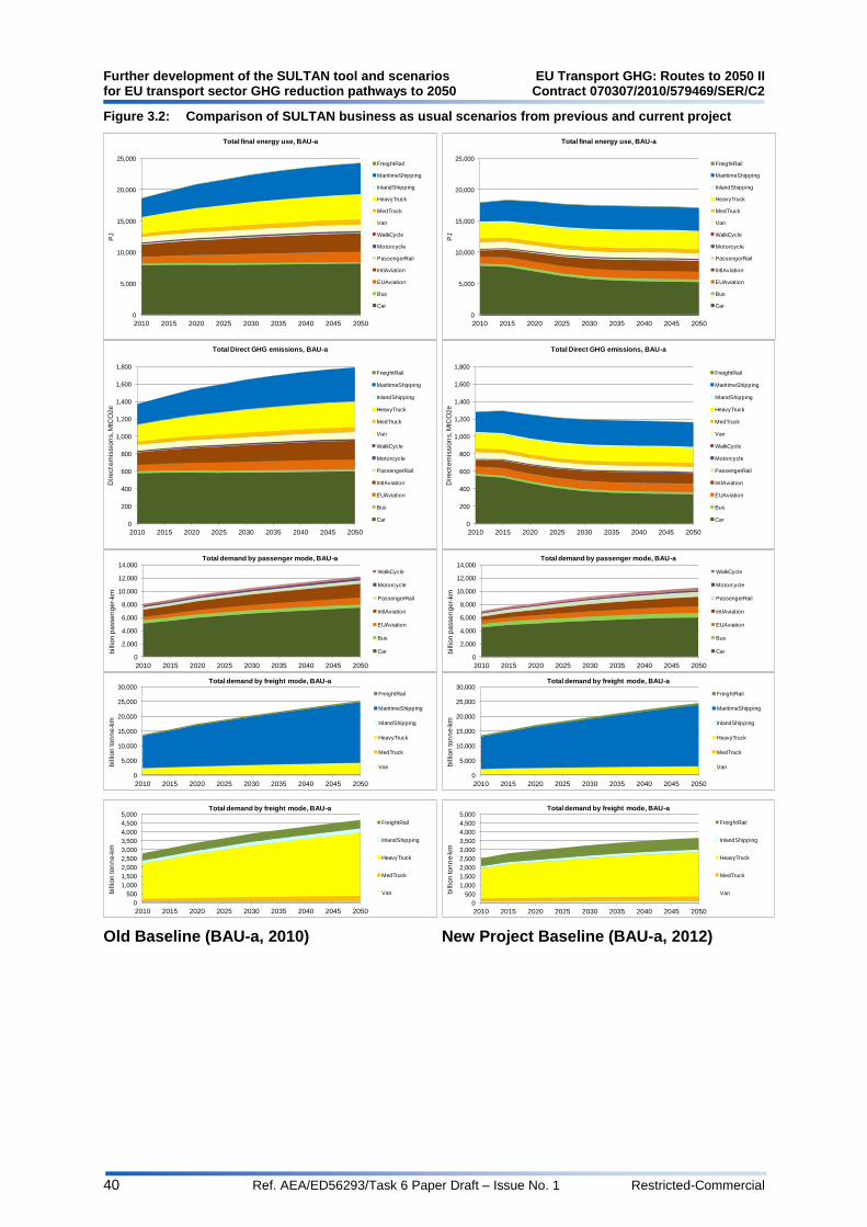
Further development of the SULTAN tool and scenarios EU Transport GHG: Routes to 2050 II for EU transport sector GHG reduction pathways to 2050 Contract 070307/2010/579469/SER/C2
40 Ref. AEA/ED56293/Task 6 Paper Draft – Issue No. 1 Restricted-Commercial
Figure 3.2: Comparison of SULTAN business as usual scenarios from previous and current project
0
5,000
10,000
15,000
20,000
25,000
2010 2015 2020 2025 2030 2035 2040 2045 2050
PJ
Total final energy use, BAU-a
FreightRail
MaritimeShipping
InlandShipping
HeavyTruck
MedTruck
Van
WalkCycle
Motorcycle
PassengerRail
IntlAviation
EUAviation
Bus
Car
0
5,000
10,000
15,000
20,000
25,000
2010 2015 2020 2025 2030 2035 2040 2045 2050
PJ
Total final energy use, BAU-a
FreightRail
MaritimeShipping
InlandShipping
HeavyTruck
MedTruck
Van
WalkCycle
Motorcycle
PassengerRail
IntlAviation
EUAviation
Bus
Car
0
200
400
600
800
1,000
1,200
1,400
1,600
1,800
2010 2015 2020 2025 2030 2035 2040 2045 2050
Dir
ect e
mis
sio
ns, M
tCO
2e
Total Direct GHG emissions, BAU-a
FreightRail
MaritimeShipping
InlandShipping
HeavyTruck
MedTruck
Van
WalkCycle
Motorcycle
PassengerRail
IntlAviation
EUAviation
Bus
Car
0
200
400
600
800
1,000
1,200
1,400
1,600
1,800
2010 2015 2020 2025 2030 2035 2040 2045 2050
Dir
ect e
mis
sio
ns, M
tCO
2e
Total Direct GHG emissions, BAU-a
FreightRail
MaritimeShipping
InlandShipping
HeavyTruck
MedTruck
Van
WalkCycle
Motorcycle
PassengerRail
IntlAviation
EUAviation
Bus
Car
0
2,000
4,000
6,000
8,000
10,000
12,000
14,000
2010 2015 2020 2025 2030 2035 2040 2045 2050
billio
n p
asse
ng
er-
km
Total demand by passenger mode, BAU-a
WalkCycle
Motorcycle
PassengerRail
IntlAviation
EUAviation
Bus
Car
0
2,000
4,000
6,000
8,000
10,000
12,000
14,000
2010 2015 2020 2025 2030 2035 2040 2045 2050
billio
n p
asse
ng
er-
km
Total demand by passenger mode, BAU-a
WalkCycle
Motorcycle
PassengerRail
IntlAviation
EUAviation
Bus
Car
0
5,000
10,000
15,000
20,000
25,000
30,000
2010 2015 2020 2025 2030 2035 2040 2045 2050
billio
n to
nn
e-k
m
Total demand by freight mode, BAU-a
FreightRail
MaritimeShipping
InlandShipping
HeavyTruck
MedTruck
Van
0
5,000
10,000
15,000
20,000
25,000
30,000
2010 2015 2020 2025 2030 2035 2040 2045 2050
billio
n to
nn
e-k
m
Total demand by freight mode, BAU-a
FreightRail
MaritimeShipping
InlandShipping
HeavyTruck
MedTruck
Van
0
500
1,000
1,500
2,000
2,500
3,000
3,500
4,000
4,500
5,000
2010 2015 2020 2025 2030 2035 2040 2045 2050
billio
n to
nn
e-k
m
Total demand by freight mode, BAU-a
FreightRail
InlandShipping
HeavyTruck
MedTruck
Van
0
500
1,000
1,500
2,000
2,500
3,000
3,500
4,000
4,500
5,000
2010 2015 2020 2025 2030 2035 2040 2045 2050
billio
n to
nn
e-k
m
Total demand by freight mode, BAU-a
FreightRail
InlandShipping
HeavyTruck
MedTruck
Van
Old Baseline (BAU-a, 2010) New Project Baseline (BAU-a, 2012)

EU Transport GHG: Routes to 2050 II Further development of the SULTAN tool and scenarios Contract 070307/2010/579469/SER/C2 for EU transport sector GHG reduction pathways to 2050
Restricted-Commercial Ref. AEA/ED56293/Task 6 Paper Draft – Issue No. 1 41
Figure 3.3: Comparison of the SULTAN business as usual scenarios from current and previous projects
0
200
400
600
800
1,000
1,200
1,400
1,600
1,800
2,000
2,200
2010 2015 2020 2025 2030 2035 2040 2045 2050
Co
mb
ine
d (life
cy
cle
) e
mis
sio
ns
, M
tCO
2e
Total Combined (life cycle) GHG emissions, BAU-a
FreightRail
MaritimeShipping
InlandShipping
HeavyTruck
MedTruck
Van
WalkCycle
Motorcycle
PassengerRail
IntlAviation
EUAviation
Bus
Car
Total WP Targets
SULTAN 2010 BAU
Notes: The ‘Total WP Targets’ figure indicated includes both the goal of reducing maritime emissions by 40% by 2050, as well as the targets for the rest of transport in 2030 and 2050. The error bars on these points represent the range of values for these targets that were indicated in the 2050 Roadmap.
The primary differences between the SULTAN 2012 and SULTAN 2010 baselines (illustrated in Figure 3.2 and Figure 3.3) are summarised as follows, with a more detailed summary of their impacts provided in the following paragraphs:
a) Lower 2010 starting point reflecting the impacts of the recession (not included in the previous Commission modelling baseline). The impacts of the recent global recession, which have been factored into the modelling (at least in terms of impacts to 2010), could be expected to have a reasonably significant impact on 2020 GHG, but a relatively very minor contribution by 2050.
b) Inclusion of 2020 regulatory CO2 targets for new cars (95gCO2/km) and vans (147gCO2/km) - only the 2015/17 targets were included in the baseline previously;
c) Aviation activity and energy consumption has been scaled to international bunkers, rather than full flight distance to/from EU countries (i.e. excludes transfers/multi-leg components refuelling outside EU). This is to maintain consistency with the PRIMES modelling used as the basis of the 2050 Roadmap and Transport White Paper analysis and targets.
d) Shipping energy consumption/GHG emissions now factor in the IMO’s new Energy Efficiency Design Index (EEDI) targets for new vessel efficiency;
e) Significant activity modal shifts in passenger and freight transport and a 13% reduction in non-shipping tkm by 2050 (versus the previous baseline).
f) Changes to average road vehicle lifetimes used in the modelling – summarised in Table 3.1. The average vehicle lifetimes have reduced in many cases which accelerates the uptake of new technologies (and hence impacts on GHG reduction). The difference is particularly marked for commercial vehicles, where the previous lifetimes were very high compared to European statistics.

Further development of the SULTAN tool and scenarios EU Transport GHG: Routes to 2050 II for EU transport sector GHG reduction pathways to 2050 Contract 070307/2010/579469/SER/C2
42 Ref. AEA/ED56293/Task 6 Paper Draft – Issue No. 1 Restricted-Commercial
Table 3.1: Comparison of average road vehicle lifetimes from the previous and new SULTAN versions
Old SULTAN (2010) Updated SULTAN (2012) % Change
Car 14 12 -14%
Bus 17 12 -29%
Motorcycle 25 13 -48%
Van 20 12 -40%
Med Truck 20 11 -45%
Heavy Truck 20 10 -50%
Source: SULTAN Illustrative Scenarios Tool
Notes: The derived average vehicle lifetimes used in both the previous and updated versions of SULTAN are based on data from the TREMOVE 2.7 and TREMOVE 3.3.1 model versions respectively.
Passenger Cars:
Direct emissions of GHG from passenger cars have reduced by 125 Mtonne CO2e (21%) in 2020, and by 264 Mtonne CO2e (44%) in 2050, comparing the 2012 BAU versus the 2010 BAU. This change appears to be mainly driven by a combination of several significant changes between the two baselines. Firstly, there is a marked reduction in passenger car activity (15% in 2020, and 20% in 2050), which appears to be mainly due to significant modal shift to both buses and passenger rail, which in the new baseline have increased by 47% and 58% respectively by 2050 relative to the previous baseline. The second significant effect is the inclusion of the 2020 regulatory new car target of 95gCO2/km within the new baseline (only 2015 target was included previously), which is anticipated to account for the majority of the remaining difference (~6% reduction in GHG in 2020, 24% by 2050). A small reduction in the average vehicle lifetime in the Commission’s modelling (see Table 3.1) will also have a further contributory effect; however this is likely to be relatively small. Vans:
Direct emissions of GHG from vans have reduced by 3.1 Mtonne CO2e (4.4%) in 2020, and by 20.1 Mtonne CO2e (25.7%) in 2050, comparing the 2012 BAU versus the 2010 BAU. This change appears to be mainly driven principally by two factors. First, there has been a significant reduction (40%) in the average vehicle lifetime in the Commission’s modelling (see Table 3.1), which is likely to have had a major effect on the rate of fleet efficiency improvements, particularly for 2050. The inclusion of the 2020 regulatory new van target of 147gCO2/km within the new baseline (only 2015 target was included previously), is anticipated to also account for the much of the difference in 2020 but to a lesser degree by 2050 where the overall lifetime change would be expected to be larger. In 2020 the new baseline also has 7% higher tonne km from vans, however this difference drops to around 1.5% by 2050. Medium/Heavy Trucks:
Emissions of GHG from medium/heavy trucks have reduced by 6/58 Mtonne CO2e (14%/25%) respectively in 2020, and by 16/115 Mtonne CO2e (28%/39%) in 2050, comparing the 2012 BAU versus the 2010 BAU. This change appears to be mainly driven by a combination of several significant changes between the two baselines. Firstly, there is a marked reduction in medium/heavy truck activity (7% in 2020, and 24%/36% in 2050), which appears to be mainly due to significant modal shift to freight rail, which in the new baseline has increased by 39% by 2050 relative to the previous baseline (but is also 8% higher in 2010). The second significant effect is a reduction in the average vehicle lifetime in the Commission’s modelling (see Table 3.1) for medium/heavy trucks (45%/50% respectively). This is likely to have had a significant effect on the rate of fleet efficiency improvements, for 2050. Finally, amendments to the assumed new vehicle efficiency improvements have been made to all heavy duty vehicle categories, reflecting the findings of work completed by AEA for the European Commission in early 2011, which considered the potential for GHG reductions from HDVs to 2030 (AEA, 2011). The result of this is a lower rate of improvement

EU Transport GHG: Routes to 2050 II Further development of the SULTAN tool and scenarios Contract 070307/2010/579469/SER/C2 for EU transport sector GHG reduction pathways to 2050
Restricted-Commercial Ref. AEA/ED56293/Task 6 Paper Draft – Issue No. 1 43
in new vehicle efficiency in the new SULTAN 2012 BAU, counteracting to an extent the decrease in average vehicle lifetime in the longer term. Aviation:
The baselines for the SULTAN 2010 and SULTAN 2012 models are not directly comparable for aviation due to its revised definition - i.e. as indicated earlier the new BAU is scaled directly to European activity statistics and international bunker fuels (and has around 25% lower GHG in 2010, mainly due to this aspect). It is therefore difficult to draw conclusions on the impacts of additional policy measures (e.g. inclusion of aviation in the EU ETS) through comparison of the baselines. However, one significant change that has occurred is an increase in the average new aircraft efficiency improvement assumed in the baseline. This has increased from an annual rate of efficiency improvement of 1% to a rate of improvement of 1.5% through to 2050, which is also consistent with commitments to such improvements announced by the International Air Transport Association (IATA, 2010)14. Maritime Shipping:
Emissions of GHG from medium/heavy trucks have reduced by 26 Mtonne CO2e (8.7%) in 2020, and by 110 Mtonne CO2e (28.3%) in 2050, comparing the 2012 BAU vs the 2010 BAU. Maritime shipping include estimates for the full emissions resulting from journeys to EU countries, rather than current international reporting which only include emissions from bunker fuels supplied at a country level (which are lower). This is unchanged between the two baselines, with the difference entirely due to inclusion of assumptions on the impact on new ship efficiency of the EEDI targets for maritime shipping. New ships will be required to meet a minimum level of energy efficiency, with ships built between 2015-2019 improving their efficiency by 10%, rising to 15-20% between 2020 and 2024 (depending on the ship type), and 30% for ships delivered after 2024 (T&E, 2011)15. The following Figure 3.4 presents both the overall cumulative emissions profiles of the SULTAN 2010 BAU, the 2012 BAU and the core GHG reduction scenario, as well as the cumulative totals over 5-year periods through to 2050. The latter presentation is helpful in the context of investigating possible carbon budgets at the EU-level (i.e. analogous to those developed under the Climate Change Act in the UK). This aspect is discussed in more detail in the Task 7 paper, which also explores the future impacts of early policy actions (i.e. those put in place prior to 2020). The difference in cumulative GHG emissions between the two BAU scenarios is quite substantial: ~18,000 Mtonne CO2e (24%) reduction by 2050, the lower starting point in 2010 due to the global recession may be responsible for a significant part of this difference. Options that cause a more rapid impact (e.g. the impact of the global recession reducing the rate of activity growth) can have a more significant impact on cumulative emissions than those that take time to be taken up to significant levels (e.g. deployment of new technologies into the new vehicle fleet). Therefore from the perspective of cumulative emissions, options that can achieve rapid deployment at lower % savings could still save more GHG in the long-run than those with much higher in year potential savings in the long term.
14
IATA Fact Sheet: Environment, accessed March 2011: http://www.iata.org/pressroom/facts_figures/fact_sheets/pages/environment.aspx 15
‘Environmental groups welcome IMO's energy efficiency standard for new ship, but call for further actions to reduce GHG emissions from shipping’, accessed from the T&E website on 9/02/2012: http://www.transportenvironment.org/press/environmental-groups-welcome-imos-energy-efficiency-standard-new-ship-call-further-actions

Further development of the SULTAN tool and scenarios EU Transport GHG: Routes to 2050 II for EU transport sector GHG reduction pathways to 2050 Contract 070307/2010/579469/SER/C2
44 Ref. AEA/ED56293/Task 6 Paper Draft – Issue No. 1 Restricted-Commercial
Figure 3.4: Cumulative emissions profiles for SULTAN 2010 BAU and SULTAN 2012 BAU scenarios
0
10,000
20,000
30,000
40,000
50,000
60,000
70,000
80,000
2010 2015 2020 2025 2030 2035 2040 2045 2050
Co
mb
ine
d (life
cycle
) e
mis
sio
ns, M
tCO
2e
Total cumulative GHG emissions, 2010-2050, BAU-a (2010)
FreightRail
MaritimeShipping
InlandShipping
HeavyTruck
MedTruck
Van
WalkCycle
Motorcycle
PassengerRail
IntlAviation
EUAviation
Bus
Car
BAU-a (2010)
0
1,000
2,000
3,000
4,000
5,000
6,000
7,000
8,000
9,000
10,000
11,000
Co
mb
ine
d (life
cycle
) e
mis
sio
ns, M
tCO
2e
Total 5-year cumulative emissions, 2010-2050, BAU-a (2010)
FreightRail
MaritimeShipping
InlandShipping
HeavyTruck
MedTruck
Van
WalkCycle
Motorcycle
PassengerRail
IntlAviation
EUAviation
Bus
Car
BAU-a (2010)
SULTAN 2010 Baseline
0
10,000
20,000
30,000
40,000
50,000
60,000
70,000
80,000
2010 2015 2020 2025 2030 2035 2040 2045 2050
Co
mb
ine
d (life
cycle
) e
mis
sio
ns, M
tCO
2e
Total cumulative GHG emissions, 2010-2050, BAU-a
FreightRail
MaritimeShipping
InlandShipping
HeavyTruck
MedTruck
Van
WalkCycle
Motorcycle
PassengerRail
IntlAviation
EUAviation
Bus
Car
BAU-a (2010)
0
1,000
2,000
3,000
4,000
5,000
6,000
7,000
8,000
9,000
10,000
11,000
Co
mb
ine
d (life
cycle
) e
mis
sio
ns, M
tCO
2e
Total 5-year cumulative emissions, 2010-2050, BAU-a
FreightRail
MaritimeShipping
InlandShipping
HeavyTruck
MedTruck
Van
WalkCycle
Motorcycle
PassengerRail
IntlAviation
EUAviation
Bus
Car
BAU-a (2010)
SULTAN 2012 Baseline
Source: SULTAN Illustrative Scenarios Tool, updated for the EU Transport GHG: Routes to 2050 II project
3.2 Updating the Original Scenarios
In order for them to be consistent with the new SULTAN BAU-a scenario it was necessary to update the scenarios developed in the previous project. The findings of Task 3 (knock-on consequences of policy actions16) were also taken into consideration in the updates. However, there were no new quantified findings identified that suggested changes were necessary to the existing assumptions used to define the original scenarios. The following Table 3.2 provides a summary of the final set of scenarios that were defined and modelled using SULTAN in the previous project, together with their impact area and type. Full details of the data sources and assumptions used in developing these scenarios were provided in Report VII of the previous project17. There were potentially a very wide range of different scenarios and variants that could have been investigated. However, it was not possible to investigate all promising options. The scenario coverage therefore focused attention on key policies, objectives or measures where: a) They were likely to have a significant (positive) impact on transport GHG emissions
reductions in the 2050 timeframe; b) It was possible to effectively quantify likely impacts within the SULTAN framework (e.g.
impacts on demand, vehicle efficiency, energy carrier carbon intensity, powertrain technology switching, modal switch, etc.);
16
Richard Smokers, Ian Skinner, Huib van Essen et al (2012) Exploration of the likely knock-on consequences of relevant potential policies. Task 3 paper produced as part of a contract between European Commission Directorate-General Climate Action and AEA Technology plc; see website www.eutransportghg2050.eu 17
Hill, N., Morris, M. and Skinner, I. (2010) SULTAN: Development of an Illustrative Scenarios Tool for Assessing Potential Impacts of Measures on EU Transport GHG. Task 9 Report VII produced as part of contract ENV.C.3/SER/2008/0053 between European Commission Directorate-General Environment and AEA Technology plc; see website www.eutransportghg2050.eu

EU Transport GHG: Routes to 2050 II Further development of the SULTAN tool and scenarios Contract 070307/2010/579469/SER/C2 for EU transport sector GHG reduction pathways to 2050
Restricted-Commercial Ref. AEA/ED56293/Task 6 Paper Draft – Issue No. 1 45
c) There was sufficient information / evidence identified on their potential application and impacts (OR it was possible to make reasonable estimates) in order to build a set of suitable assumptions for their assessment;
d) They impacted in a significantly different way to the other scenarios to be assessed.
Table 3.2: Summary list of the illustrative scenarios defined in SULTAN for the previous project
ID Scenarios defined in SULTAN Area Type
Single Scenarios 1 Reduce GHG intensity of fuel (all modes) A Technical
2 Mandatory new vehicle emission limits (all modes, incl./excl. biofuel) A, B
3 Package of cycling and walking improvement measures (walk/cycle) C Non-Technical 4 Improved spatial planning (road and rail)
5 Package of mobility management measures incl. improved public transport
6 Improved freight intermodality (road, rail and inland shipping)
7 Improved speed enforcement (road) D, (E)
8 Harmonised EU motorway speed limit (road)
9 Fuel-efficient driver (FED) training (road, rail)
10 Company car tax reform (cars) (A, B, C, D,) E 11 CO2 price tax (all modes, based on central/low/high CO2 costs))
12 Non-CO2 price tax (road, internalise cost of NOx, PM and energy security
13 Equivalent duty and VAT rates for fuels (all modes)
Combination Scenarios C1 Technical Measures: Reduce energy GHG intensity (biofuels) A Technical
C2 (All) Technical Measures: Mandatory new vehicle limits + biofuels A, B
C3 Scenario C2 + Spatial planning and modal shift measures A, B, C Technical and Non-Technical
C4 Scenario C3 + Speed and driver training measures A, B, C, D
C5 Scenario C4 + Taxes (with central/low/high CO2 prices), i.e. All Technical and Non-Technical Measures Scenario
A, B, C, D, E
C6 Non-Technical Measures: Planning +modal shift +speed +FED training +Tax (central/low/high CO2 prices)
C, D, E Non-Technical
Notes:
(A) Decarbonising energy carriers (i.e. reducing the GHG intensity of transport energy) (B) Improving vehicle efficiency (i.e. improving the technical energy efficiency of new vehicles) (C) Efficient organisation of transport system (i.e. improving the structural efficiency of the transport system
via modal shift, co-modality and spatial planning) (D) Improving vehicle use (i.e. using vehicles more efficiently by improving operational efficiency) (E) System efficiency (e.g. improving the economic efficiency of transport via economic instruments, by
internalising selected external costs, removing subsidies and creating a level playing field)
Many of the scenario options will affect more than one category to a greater or lesser extent, however they have been grouped in the above table into their primary category area of action.
3.3 New Simple Scenarios
A number of new options for simple scenarios were identified early in the project in order to supplement those already developed as part of the previous project, and also to help explore some of the additional issues identified in other project tasks. One of the significant areas that was not covered in the previous project included the potential for improvement to maritime shipping efficiency other than improvements to new ships (e.g. as included in the IMO’s Energy Efficiency Design Index regulations). In addition it was also deemed valuable to develop an alternative scenario for the future development of the GHG intensity of each of the SULTAN energy carriers, partly based on the assessment carried out in Task 5 on risks and uncertainties of options18. Finally, Task 4 of the project19 also highlighted the
18
Richard Smokers, Ian Skinner, Bettina Kampman et al. (2012) Identification of the major risks/uncertainties associated with the achievability of considered policies and measures. Task 5 paper produced as part of a contract between European Commission Directorate-General Climate Action and AEA Technology plc; see website www.eutransportghg2050.eu
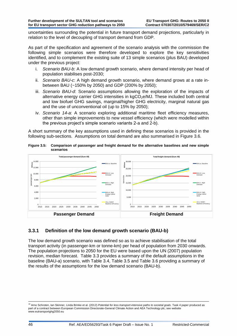
Further development of the SULTAN tool and scenarios EU Transport GHG: Routes to 2050 II for EU transport sector GHG reduction pathways to 2050 Contract 070307/2010/579469/SER/C2
46 Ref. AEA/ED56293/Task 6 Paper Draft – Issue No. 1 Restricted-Commercial
uncertainties surrounding the potential in future transport demand projections, particularly in relation to the level of decoupling of transport demand from GDP. As part of the specification and agreement of the scenario analysis with the commission the following simple scenarios were therefore developed to explore the key sensitivities identified, and to complement the existing suite of 13 simple scenarios (plus BAU) developed under the previous project:
i. Scenario BAU-b: A low demand growth scenario, where demand intensity per head of population stabilises post-2030;
ii. Scenario BAU-c: A high demand growth scenario, where demand grows at a rate in-between BAU (~150% by 2050) and GDP (200% by 2050);
iii. Scenario BAU-d: Scenario assumptions allowing the exploration of the impacts of alternative energy carrier GHG intensities in kgCO2e/MJ. These included both central and low biofuel GHG savings, marginal/higher GHG electricity, marginal natural gas and the use of unconventional oil (up to 15% by 2050);
iv. Scenario 14-a: A scenario exploring additional maritime fleet efficiency measures, other than simple improvements to new vessel efficiency (which were modelled within the previous project’s simple scenario variants 2-a and 2-b).
A short summary of the key assumptions used in defining these scenarios is provided in the following sub-sections. Assumptions on total demand are also summarised in Figure 3.6.
Figure 3.5: Comparison of passenger and freight demand for the alternative baselines and new simple scenarios
0
2,000
4,000
6,000
8,000
10,000
12,000
14,000
2010 2015 2020 2025 2030 2035 2040 2045 2050
pa
sse
ng
er-
km
Bil
lio
ns
Total passenger demand (Sum All)
BAU-a: Baseline
BAU-b: Low Demand
BAU-c: High Demand
BAU-d: High Energy Carrier GHG
14-a: Addit'l Maritime Ef f iciency
0
5,000
10,000
15,000
20,000
25,000
30,000
2010 2015 2020 2025 2030 2035 2040 2045 2050
ton
ne
-km
Bil
lio
ns
Total freight demand (Sum All)
BAU-a: Baseline
BAU-b: Low Demand
BAU-c: High Demand
BAU-d: High Energy Carrier GHG
14-a: Addit'l Maritime Ef f iciency
Passenger Demand Freight Demand
3.3.1 Definition of the low demand growth scenario (BAU-b)
The low demand growth scenario was defined so as to achieve stabilisation of the total transport activity (in passenger-km or tonne-km) per head of population from 2030 onwards. The population projections to 2050 for the EU were based upon the UN (2007) population revision, median forecast. Table 3.3 provides a summary of the default assumptions in the baseline (BAU-a) scenario, with Table 3.4, Table 3.5 and Table 3.6 providing a summary of the results of the assumptions for the low demand scenario (BAU-b).
19
Arno Schroten, Ian Skinner, Linda Brinke et al. (2012) Potential for less transport-intensive paths to societal goals. Task 4 paper produced as part of a contract between European Commission Directorate-General Climate Action and AEA Technology plc; see website www.eutransportghg2050.eu

EU Transport GHG: Routes to 2050 II Further development of the SULTAN tool and scenarios Contract 070307/2010/579469/SER/C2 for EU transport sector GHG reduction pathways to 2050
Restricted-Commercial Ref. AEA/ED56293/Task 6 Paper Draft – Issue No. 1 47
Table 3.3: EU projections in GDP, population and activity from 2010 to 2050 in the BAU-a scenario
2010 2015 2020 2030 2040 2050
GDP and Population GDP growth (per annum) 2.20% 2.20% 1.60% 1.60% 1.60% 1.60%
Population (millions) 499.4 507.7 513.8 519.9 520.1 515.3
GDP index 100% 111% 124% 146% 171% 200%
GDP/head index 100% 110% 121% 140% 164% 194%
Population index 100.0% 101. 7% 102.9% 104.1% 104.2% 103.2%
Activity Growth Total passenger-km (billions) 7,007 7,693 8,194 9,191 9,942 10,515
Total tonne-km (billions) 13,535 15,248 17,037 19,693 22,280 24,599
passenger-km index 100.0% 109.8% 116.9% 124.3% 131.2% 136.8%
tonne-km index 100.0% 112.7% 125.9% 135.4% 145.5% 155.2%
tonne-km index (excl. maritime) 100.0% 111.4% 117.7% 124.1% 129.6% 134.6%
tonne-km index (maritime) 100.0% 112.9% 127.7% 137.9% 149.1% 159.9%
Table 3.4: Indexed projections of overall activity from 2010 to 2050 resulting from the low demand growth scenario (BAU-b) assumptions
Activity Growth 2010 2015 2020 2030 2040 2050
passenger-km index 100.0% 109.8% 116.9% 131.2% 131.2% 130.0%
tonne-km index 100.0% 112.7% 125.9% 145.5% 145.5% 144.2%
tonne-km index (excl. maritime) 100.0% 111.4% 117.7% 129.6% 129.7% 128.5%
tonne-km index (maritime) 100.0% 112.9% 127.7% 149.1% 149.2% 147.8%
Table 3.5: Change in stock by mode in the low demand (BAU-b) scenario versus the baseline (BAU-a) scenario
% change on BAU-a scenario stock
2010 2015 2020 2030 2040 2050
Car 0.0% 0.0% 0.0% 0.0% -5.5% -9.2%
Bus 0.0% 0.0% 0.0% 0.0% -4.1% -7.4%
EU Aviation 0.0% 0.0% 0.0% 0.0% -11.9% -22.6%
Intl Aviation 0.0% 0.0% 0.0% 0.0% -14.4% -25.4%
Passenger Rail 0.0% 0.0% 0.0% 0.0% -10.0% -17.1%
Motorcycle 0.0% 0.0% 0.0% 0.0% -6.3% -10.8%
Walk /Cycle 0.0% 0.0% 0.0% 0.0% 0.0% 0.0%
Van 0.0% 0.0% 0.0% 0.0% -8.8% -14.8%
Medium Truck 0.0% 0.0% 0.0% 0.0% -6.9% -12.1%
Heavy Truck 0.0% 0.0% 0.0% 0.0% -6.9% -12.1%
Inland Shipping 0.0% 0.0% 0.0% 0.0% -5.2% -8.5%
Maritime Shipping 0.0% 0.0% 0.0% 0.0% -12.5% -22.2%
Freight Rail 0.0% 0.0% 0.0% 0.0% -6.8% -12.0%

Further development of the SULTAN tool and scenarios EU Transport GHG: Routes to 2050 II for EU transport sector GHG reduction pathways to 2050 Contract 070307/2010/579469/SER/C2
48 Ref. AEA/ED56293/Task 6 Paper Draft – Issue No. 1 Restricted-Commercial
Table 3.6: Change in activity by mode in the low demand (BAU-b) scenario versus the baseline (BAU-a) scenario
% change on BAU-a scenario demand
2010 2015 2020 2030 2040 2050
Car 0.0% 0.0% 0.0% 0.0% -5.5% -9.2%
Bus 0.0% 0.0% 0.0% 0.0% -4.1% -7.4%
EU Aviation 0.0% 0.0% 0.0% 0.0% -11.9% -22.6%
Intl Aviation 0.0% 0.0% 0.0% 0.0% -14.3% -25.3%
Passenger Rail 0.0% 0.0% 0.0% 0.0% -10.0% -17.1%
Motorcycle 0.0% 0.0% 0.0% 0.0% -6.3% -10.8%
Walk /Cycle 0.0% 0.0% 0.0% 0.0% -7.4% -13.8%
Van 0.0% 0.0% 0.0% 0.0% -8.8% -14.8%
Medium Truck 0.0% 0.0% 0.0% 0.0% -6.9% -12.1%
Heavy Truck 0.0% 0.0% 0.0% 0.0% -6.9% -12.1%
Inland Shipping 0.0% 0.0% 0.0% 0.0% -5.2% -8.5%
Maritime Shipping 0.0% 0.0% 0.0% 0.0% -12.5% -22.2%
Freight Rail 0.0% 0.0% 0.0% 0.0% -6.8% -12.0%
3.3.2 Definition of the high demand growth scenario (BAU-c)
The low demand growth scenario was defined so as to achieve growth rates in activity/demand in-between those of the baseline (BAU-a) scenario levels and the assumed rate of GDP growth from the PRIMES-TREMOVE reference scenario used in the 2011 White Paper analysis (see Table 3.3). Table 3.7, Table 3.8 and Table 3.9 provide a summary of the results of the assumptions for the high demand scenario (BAU-c).
Table 3.7: Indexed projections of overall activity from 2010 to 2050 resulting from the high demand growth scenario (BAU-c) assumptions
Activity Growth 2010 2015 2020 2030 2040 2050
passenger-km index 100.0% 108.9% 118.5% 136.4% 154.5% 174.8%
tonne-km index 100.0% 111.2% 123.3% 142.7% 164.3% 187.8%
tonne-km index (excl. maritime) 100.0% 110.5% 119.3% 134.8% 151.6% 169.9%
tonne-km index (maritime) 100.0% 111.3% 124.3% 144.5% 167.2% 191.9%
Table 3.8: Change in stock by mode in the high demand (BAU-c) scenario versus the baseline (BAU-a) scenario
% change on BAU-a scenario stock
2010 2015 2020 2030 2040 2050
Car 0.0% -0.8% 1.3% 4.0% 8.9% 16.5%
Bus 0.0% -0.8% 1.3% 4.0% 8.9% 16.5%
EU Aviation 0.0% -0.8% 1.3% 4.0% 8.9% 16.5%
Intl Aviation 0.0% -0.8% 1.3% 4.0% 8.9% 16.5%
Passenger Rail 0.0% -0.8% 1.3% 4.0% 8.9% 16.5%
Motorcycle 0.0% -0.8% 1.3% 4.0% 8.9% 16.5%
Walk /Cycle 0.0% -0.8% 1.3% 4.0% 8.9% 16.5%
Van 0.0% -0.8% 1.3% 4.0% 8.9% 16.5%
Medium Truck 0.0% -0.8% 1.3% 4.0% 8.9% 16.5%
Heavy Truck 0.0% -0.8% 1.3% 4.0% 8.9% 16.5%
Inland Shipping 0.0% -0.8% 1.3% 4.0% 8.9% 16.5%
Maritime Shipping 0.0% -1.5% -2.7% -3.1% -1.9% 1.1%
Freight Rail 0.0% -0.8% 1.3% 4.0% 8.9% 16.5%

EU Transport GHG: Routes to 2050 II Further development of the SULTAN tool and scenarios Contract 070307/2010/579469/SER/C2 for EU transport sector GHG reduction pathways to 2050
Restricted-Commercial Ref. AEA/ED56293/Task 6 Paper Draft – Issue No. 1 49
Table 3.9: Change in activity by mode in the high demand (BAU-c) scenario versus the baseline (BAU-a) scenario
% change on BAU-a scenario demand
2010 2015 2020 2030 2040 2050
Car 0.0% -0.8% 1.3% 4.0% 8.9% 16.5%
Bus 0.0% -0.8% 1.3% 4.0% 8.9% 16.5%
EU Aviation 0.0% -0.8% 1.3% 4.0% 8.9% 16.5%
Intl Aviation 0.0% -0.8% 1.3% 4.0% 8.9% 16.5%
Passenger Rail 0.0% -0.8% 1.3% 4.0% 8.9% 16.5%
Motorcycle 0.0% -0.8% 1.3% 4.0% 8.9% 16.5%
Walk /Cycle 0.0% -0.8% 1.3% 4.0% 8.9% 16.5%
Van 0.0% -0.8% 1.3% 4.0% 8.9% 16.5%
Medium Truck 0.0% -0.8% 1.3% 4.0% 8.9% 16.5%
Heavy Truck 0.0% -0.8% 1.3% 4.0% 8.9% 16.5%
Inland Shipping 0.0% -0.8% 1.3% 4.0% 8.9% 16.5%
Maritime Shipping 0.0% -1.5% -2.7% -3.1% -1.9% 1.1%
Freight Rail 0.0% -0.8% 1.3% 4.0% 8.9% 16.5%
3.3.3 Definition of the alternative energy carrier GHG intensity scenario (BAU-d)
The purpose of this scenario was to explore the potential implications of alternative scenarios for the future development of the GHG intensity of each SULTAN energy carriers, partly based on the findings of the assessment carried out in Task 5 on risks and uncertainties of options. In general the objective was to develop alternative ‘pessimistic’ cases for the energy carrier GHG intensities, since the existing scenario assumptions are generally quite optimistic. The considerations in the following subsections were therefore used as a basis for defining the revised values used in the BAU-d scenario.
Biofuels:
In the baseline and core GHG reduction scenario (R1-a), discussed later, the average GHG performance of liquid fuels is determined by the percentage GHG reduction (versus conventional fuels) and percentage deployment/substitution. The default assumptions previously used were for high levels of GHG savings (up to 85% by 2050) and with deployment capped at a fixed maximum amount of up to 174 Mtoe sustainable biofuel by 2050 20. The findings of Task 5 of the project indicate that there is significant uncertainty as to what the volumes of sustainable biofuel may be available in the future and the net savings (e.g. due to indirect land use change issues). Two alternative biofuel GHG savings trajectories were therefore defined (i) low savings – based on an assessment of potential net savings in the absence of further action from the EC’s draft impact assessment21 of ~10-20% due to indirect land use change (ILUC) impacts; (ii) central savings, with indicative values in between the baseline/high savings and the low savings assumptions. The corresponding biofuel GHG savings applied in different scenarios are summarised in Table 3.10.
20
The basis for the first assumption is an assessment by BIOFRAC (2006) on the 2030 potential for biofuels produced from EU sourced biomass using advanced biofuels technologies: “Biofuels in the European Union - A VISION FOR 2030 AND BEYOND”, Final draft report of the Biofuels Research Advisory Council, March 2006. Report available at: http://ec.europa.eu/research/energy/pdf/biofuels_vision_2030_en.pdf 21
Commission Working Staff Document on indirect land use change related to biofuels – impact assessment, DRAFT SEC(2011), accessed from the ENDS Europe website on 17/01/2012: http://www.endseurope.com/docs/120126b.pdf

Further development of the SULTAN tool and scenarios EU Transport GHG: Routes to 2050 II for EU transport sector GHG reduction pathways to 2050 Contract 070307/2010/579469/SER/C2
50 Ref. AEA/ED56293/Task 6 Paper Draft – Issue No. 1 Restricted-Commercial
Table 3.10: Assumptions on average biofuel GHG savings versus conventional fuels utilised in different project scenarios
Scenario 2010 2015 2020 2030 2040 2050
Biogas
Baseline Savings BAU-a 100% 100% 100% 100% 100% 100%
High Savings R1-a 100% 100% 100% 100% 100% 100%
Central Savings 55.0% 56.0% 57.0% 58.0% 59.0% 60.0%
Low Savings BAU-d 10.0% 11.3% 12.5% 15.0% 17.5% 20.0%
Other biofuels
Baseline Savings BAU-a 56.8% 66.1% 70.6% 77.0% 85.1% 88.2%
High Savings R1-a 55.0% 55.0% 60.0% 70.0% 80.0% 85.0%
Central Savings 20.0% 30.0% 35.0% 40.0% 45.0% 50.0%
Low Savings BAU-d 10.0% 11.3% 12.5% 15.0% 17.5% 20.0%
Conventional liquid fuels:
The default performance of conventional liquid fuels is based on the assumptions on direct and indirect GHG emissions per GJ fuel from the PRIMES-TREMOVE reference scenario, which remain approximately constant from 2010 to 2050 (with a small decline in indirect emissions). However, it has been suggested that if significant amounts of conventional fuels were produced from unconventional oil (e.g. from oil sands, oil shale or coal-to-liquid conversion) then this could result in a significant increase in fuel cycle/WTT emissions. According to ICCT (2010)22 the U.S. Energy Information Administration projects that 8% of the global supply will come from unconventional oil by 2035. Furthermore, recent work carried out for the European Commission has indicated that total WTW/fuel lifecycle GHG emissions of fuels produced from unconventional oil could be 23%-97% higher than those from conventional oil (T&E, 201123) (with values ranging from 107.3 gCO2e/MJ for oil sands, to 172 gCO2e/MJ for CTL). This equates to an increase in indirect/WTT GHG emissions of between 141% and 595%. For the purposes of developing alternative scenarios for conventional liquid fuels, the assumptions summarised in Table 3.11 were utilised for the increased WTT GHG emissions due to unconventional oil (conservatively on the basis of current figures for oil sands, with some improvement to 2050) and for the future utilisation of unconventional oil.
Table 3.11: Alternate conventional liquid fuels scenario assumptions for BAU-d
Unconventional Oil 2010 2015 2020 2030 2040 2050
WTT GHG as % conventional oil 241% 236% 231% 221% 210% 200%
Utilisation as % of total oil 0% 0% 2% 5% 10% 15%
Natural Gas:
In the future an increasing proportion of the natural gas supplied in Europe will be imported from other countries as more local sources are depleted. In particular, the additional/marginal natural gas supplied for transport may be sourced from further afield, with correspondingly higher WTT emission factors (mainly due to higher methane leakage rates for transporting the gas greater distances). As an alternative assumption the marginal gas WTT emission factors provided in the most recent JEC WTW report (2011)24 were therefore used (13.9 gCO2e/MJ, versus current EU mix value of 8.36 gCO2e/MJ).
22
Carbon Intensity of Crude Oil in Europe, a report by Energy-Redefined LLC for ICCT (2010). Accessed from the ICCT’s website on 17/01/2012: http://www.theicct.org/carbon-intensity-crude-oil-europe 23
“Report for Commission confirms carbon-intensity of tar sands”, a T&E news article from 11 February 2011, accessed from the T&E website on 17/01/2012: http://www.transportenvironment.org/news/report-commission-confirms-carbon-intensity-tar-sands 24
JEC - Joint Research Centre-EUCAR-CONCAWE collaboration, "Well-to-Wheels Analysis of Future Automotive Fuels and Powertrains in the European Context” Version 3c, Report EUR 24952 EN - 2011, accessed from the JEC website on 17/01/2012: http://iet.jrc.ec.europa.eu/about-jec/downloads

EU Transport GHG: Routes to 2050 II Further development of the SULTAN tool and scenarios Contract 070307/2010/579469/SER/C2 for EU transport sector GHG reduction pathways to 2050
Restricted-Commercial Ref. AEA/ED56293/Task 6 Paper Draft – Issue No. 1 51
Electricity:
The default (high) assumptions for electricity GHG emissions used in the core R1-a scenario are based on the minimum reduction in the carbon intensity of electricity production in 2050 from the Commission’s 2050 Roadmap (i.e. 93% reduction on 1990). However, should the amount of electricity needed to supply transport with energy substantially increase in the future, the additional electricity supplied for this purpose might be produced from higher GHG sources if there are difficulties in deploying additional renewable/nuclear generation options. For the alternative scenario it is assumed that the 2050 electricity GHG saving relative to 1990 is approximately equivalent to electricity production from coal with CCS (carbon capture and storage). The alternate assumptions for electricity lifecycle GHG emissions are summarised in Table 3.12 for different scenarios.
Table 3.12: Assumptions on average electricity GHG emission factors and savings versus 1990 utilised in different project scenarios
Scenario 2010 2015 2020 2030 2040 2050
Lifecycle GHG emissions in gCO2e/MJ
Baseline Savings BAU-a 112.9 102.6 99.1 79.4 49.9 30.0
High Savings R1-a 112.9 100.0 87.1 61.3 35.4 9.6
Low Savings BAU-d 112.9 104.8 96.7 80.4 64.2 48.0
Electricity % reduction on 1990
Baseline Savings BAU-a 18% 25% 28% 42% 64% 78%
High Savings R1-a 18% 27% 36% 55% 74% 93%
Low Savings BAU-d 18% 24% 29% 41% 53% 65%
Hydrogen:
The GHG intensity of hydrogen is currently based upon a transition from 100% hydrogen production from natural gas in 2010, to 100% production from electricity by 2050. The alternate scenario assumptions for hydrogen are based on the same transition but using the alternative scenario assumptions for natural gas and electricity. The alternate assumptions for hydrogen lifecycle GHG emissions are summarised in Table 3.13 for different scenarios.
Table 3.13: Assumptions on average hydrogen GHG emission factors utilised in different project scenarios
Scenario 2010 2015 2020 2030 2040 2050
Lifecycle GHG emissions in gCO2e/MJ
Baseline Savings BAU-a 101.8 103.3 104.3 104.2 75.5 41.6
High Savings R1-a 97.4 98.9 98.7 91.3 58.3 13.3
Low Savings BAU-d 106.2 106.2 106.1 104.3 95.5 66.6
3.3.4 Definition of the maritime fleet efficiency measures scenario (14-a)
Potential future improvements to new vessel efficiency have been previously modelled within the previous project’s simple scenario variants 2-a and 2-b (and in combination scenarios). However, there are also a wide range of efficiency improvement/GHG reduction options that have been identified in the literature (e.g. IMO, 200925) that could be applied to improve the overall efficiency of the maritime shipping fleet – including both technical measures acting on ship efficiency (e.g. through retrofit to existing ships) and operational and other non-technical measures (e.g. fleet management, speed reduction, improved logistical efficiency, ‘voyage optimisation’, etc) acting on ship efficiency, as well as on load factors and overall tonne-km activity (e.g. through more direct routing reducing overall ship km travelled, more localised
25
IMO (2009). Buhaug, Ø., Corbett, J.J., Endresen, Ø., Eyring, V., Faber, J., Hanayama, S., Lee, D.S., Lee, D., Lindstad, H., Markowska, A.Z., Mjelde, A., Nelissen, D., Nilsen, J., Pålsson, C.,Winebrake, J.J., Wu, W.–Q.,Yoshida, K. (2009). Second IMO GHG study 2009, International Maritime Organization (IMO), London, UK, April 2009.

Further development of the SULTAN tool and scenarios EU Transport GHG: Routes to 2050 II for EU transport sector GHG reduction pathways to 2050 Contract 070307/2010/579469/SER/C2
52 Ref. AEA/ED56293/Task 6 Paper Draft – Issue No. 1 Restricted-Commercial
sourcing of products, etc). Examples of the levels of potential GHG savings attributed to ship operational measures from the IMO (2009) report are provided in Table 3.14.
Table 3.14: Summary of estimates for potential reductions in CO2 emissions from maritime shipping due to operational measures from IMO (2009)
OPERATION (All ships) Saving of CO2/tonne-mile Combined
Fleet management, logistics and incentives 5% to 50%
10% to 50% Voyage optimisation 1% to 10%
Energy management 1% to 10%
This scenario was therefore developed to help exploring the potential for these additional maritime fleet efficiency measures. Table 3.15 provides a summary of the results of the indicative assumptions for the maritime fleet efficiency measures scenario (14-a).
Table 3.15: Summary of assumed impacts on maritime shipping fleet efficiency, overall demand and load factors for scenario 14-a
Maritime Shipping 2010 2015 2020 2030 2040 2050
Improvement in fleet efficiency 0% 0% 2.5% 5.0% 7.5% 10.0%
Change in BAU demand/activity, tkm 0% 0% -1.0% -2.0% -3.0% -5.0%
Change in BAU load factor 0% 0% 2.5% 5.0% 7.5% 10.0%
3.4 Routes to 2050 Scenarios
As part of the project’s central scenario analysis a series of 5 core scenario packages/sensitivities were agreed with the Commission to explore key risks and uncertainties identified in other project tasks (i.e. Task 3, 4 and 5) in relation to meeting the EU’s overall target for GHG reduction by 2050 in the transport sector. A central Core GHG Reduction Scenario (R1) was developed to for the basis for the sensitivity analyses carried out for Task 6, as well as that carried out for Task 7 and the Task 11 ad-hoc analysis. This core scenario was developed according to the following general principals: 1) It was designed to achieve White Paper’s 60% GHG reduction target (on 1990 levels) for
transport excluding maritime shipping by 2050, and goal of 40% reduction in maritime shipping GHG (on 2005 levels) (R1-a = lifecycle GHG basis; R1-b = direct GHG basis);
2) Lower conventional fuel prices were used versus the baseline (BAU-a) scenario, consistent with the White Paper’s Impact Assessment Global Decarbonisation Scenario (provided by the Commission). A degree of rebound (in activity and increased vehicle energy consumption) resulting from these lower prices was factored into the calculations;
3) 2050 targets were assumed to be achieved through predominantly technical measures, plus additional measures broadly consistent with other White Paper Goals (e.g. internalising of external costs, additional shift of road freight transport to rail/IWW);
The methodology employed in carrying out the analysis was to take the core R1-a scenario as a basis and explore sensitivities in relation to this scenario:
a) Energy Carrier Sensitivities: The potential impacts of key energy carrier / technology risks and uncertainties identified in Task 5 were explored with scenarios R2 and R3 - potential impacts of low biofuel GHG savings and low biofuel AND low electricity GHG savings, respectively;
b) Demand Sensitivities: The potential impacts of variances in the growth of activity demand identified in Task 4 were explored with scenarios R4 and R5 (low and high demand scenarios respectively);
For the analysis a two-stage process was utilised for exploring potential implications:

EU Transport GHG: Routes to 2050 II Further development of the SULTAN tool and scenarios Contract 070307/2010/579469/SER/C2 for EU transport sector GHG reduction pathways to 2050
Restricted-Commercial Ref. AEA/ED56293/Task 6 Paper Draft – Issue No. 1 53
(1) First amend the R1-a scenario assumptions for the area being explored to discover the resulting gap to reach the 2050 GHG emission targets;
(2) Re-adjust the scenario to again meet 2050 GHG targets by adding/strengthening or removing/relaxing GHG mitigation options as appropriate.
The following sub-sections provide further details on the definition of these five central ‘Routes to 2050’ scenarios.
3.4.1 Definition of the Core GHG Reduction Scenario (R1-a)
As part of the main scenario analysis work carried out for the project a ‘Core GHG Reduction Scenario’ has been developed to be broadly consistent with the targets and goals included in the 2050 Roadmap, the Transport White Paper, and supporting Commission modelling. The resulting GHG trajectory for this core scenario (R1a) is presented in the following Figure 3.6, in comparison to the business as usual scenario.
Figure 3.6: Comparison of the baseline (BAU-a) and Core GHG reduction scenario (R1-a) developed for the current project in the context of the Transport White Paper and 2050 Roadmap targets
0
200
400
600
800
1,000
1,200
1,400
1,600
1,800
2010 2015 2020 2025 2030 2035 2040 2045 2050
Co
mb
ine
d (life
cycle
) e
mis
sio
ns, M
tCO
2e
Total Combined (life cycle) GHG emissions, R1-a
FreightRail
MaritimeShipping
InlandShipping
HeavyTruck
MedTruck
Van
WalkCycle
Motorcycle
PassengerRail
IntlAviation
EUAviation
Bus
Car
BAU-a total
Total WP Targets
Source: SULTAN Illustrative Scenarios Tool, updated for the EU Transport GHG: Routes to 2050 II project
Notes: The error bars on the Total White Paper Targets indicators represent the upper and lower bound for the transport GHG reduction targets from the 2050 Roadmap. Since Maritime Shipping targets are only included in the Transport White Paper (and separately to the rest of transport), the indicative range assumed for these has been estimated on a consistent basis as those for the rest of transport.
The following Table 3.16 provides a summary of the key assumptions used to define the Core GHG Reduction Scenario (R1-a), with the corresponding technology penetration shares for different modes presented in Figure 3.7. In addition, the assumptions in non-powertrain technology improvements to new vehicle and all fleet efficiencies (relative to the baseline) are summarised in Table 3.17. Furthermore a summary of the external costs of CO2, NOx and PM emissions is presented in Table 3.18 and Table 3.19. These assumptions are based on information from the EC’s IMPACT project. In addition an indicative figure for energy security from the IMPACT handbook of approximately 5 €cent/litre has also been utilised.

Further development of the SULTAN tool and scenarios EU Transport GHG: Routes to 2050 II for EU transport sector GHG reduction pathways to 2050 Contract 070307/2010/579469/SER/C2
54 Ref. AEA/ED56293/Task 6 Paper Draft – Issue No. 1 Restricted-Commercial
Table 3.16: Summary of key assumptions in the Core GHG Reduction Scenario (R1-a) meeting the White Paper main GHG reduction targets/objectives
# Area Summary of key assumptions
GHG emissions
1 All except maritime R1-a - meets 60% reduction target relative to 1990) on a LIFECYCLE GHG basis
2 Maritime Shipping R1-a - meets 40% reduction target (relative to 2005) on a LIFECYCLE GHG basis
3 All R1-b - as for R1a, but targets met on a DIRECT GHG emissions basis (some adjustment/loosening of further assumptions below was necessary).
New vehicle GHG targets
1 Car ~80% reduction lifecycle GHG on 2010 (on basis of low biofuel savings)*
2 Bus ~80% reduction lifecycle GHG on 2010 (on basis of low biofuel savings)*
3 EU Aviation WP baseline 1.5% p.a. improvement in efficiency
4 International Aviation WP baseline 1.5% p.a. improvement in efficiency
5 Passenger Rail WP baseline move to almost 100% electric new passenger rail by 2050
6 Motorcycle ~70% reduction lifecycle GHG on 2010 (on basis of low biofuel savings)*
7 Walk-Cycle N/A
8 Van ~80% reduction lifecycle GHG on 2010 (on basis of low biofuel savings)*
9 Medium Truck ~75% reduction lifecycle GHG on 2010 (on basis of low biofuel savings)*
10 Heavy Truck ~60% reduction lifecycle GHG on 2010 (on basis of low biofuel savings)*
11 Inland Shipping ~50% reduction lifecycle GHG on 2010 (on basis of low biofuel savings)**
12 Maritime Shipping ~55% reduction lifecycle GHG on 2010 (on basis of low biofuel savings)**
13 Freight Rail White Paper modelling baseline move to 95% electric new freight rail by 2050
Fleet efficiency
1 Maritime Shipping Operational efficiency - across fleet resulting in up to 8% energy efficiency improvements by 2050
2 Maritime Shipping Operational efficiency - load factors increase to 10% over BAU by 2050
3 Road Increase in average load factor from up to 5% by 2050
Energy carriers
1 All biofuels High biofuel GHG savings by 2050 (rising from 55% in 2010 to 85% by 2050)
2 Road +Rail +Inl’dShip 50% biofuels substituting conventional fuels by 2050
3 Maritime Shipping 40% biofuels substituting conventional fuels by 2050
4 Air 40% biofuels substituting conventional fuels by 2050 (WP target)
Road speeds and driver training
1 Road transport No additional speed constraints over BAU
2 Road transport No driver training
Modal shift, spatial planning and demand (operational efficiency)
1 Passenger Additional low level shift from cars to public transport/slow modes after 2020 - rising up to 10% by 2050 in urban areas, 3% for rural/motorway.
2 Freight Additional shift of tkm from Heavy Trucks to Rail/Inland Shipping - rising to 20% in 2050 for motorway traffic and 5% for extra-urban traffic.
Fuel taxes
1 All modes Fuel Prices based on WP analysis 'Global decarbonisation' scenario, leading to some rebound in activity/efficiency versus baseline
2 All modes GHG and AQ external costs internalised and added to energy carrier cost
3 All modes Start to harmonise all fuel taxes (incl. aviation and maritime), 25% by 2050
Other
1 Cars Company car tax reform (previous project scenario 10a assumptions)
Notes: * Predominantly achieved by adjusting technology mix for new vehicles, balance of BEVs and H2 FCEVs
** Partly based on shift in technology split (some LNG, Wind), partly on increased rate of general new ship efficiency improvement


Further development of the SULTAN tool and scenarios EU Transport GHG: Routes to 2050 II for EU transport sector GHG reduction pathways to 2050 Contract 070307/2010/579469/SER/C2
56 Ref. AEA/ED56293/Task 6 Paper Draft – Issue No. 1 Restricted-Commercial
Figure 3.7: New vehicle technology penetration assumptions included in the Core Scenario (R1-a)
0%
10%
20%
30%
40%
50%
60%
70%
80%
90%
100%
2010 2015 2020 2030 2040 2050
New
Fle
et
Sh
are
, %
Car
CNG
LPG
FCEV
EV
PHEV diesel
PHEV gasoline
HEV diesel
HEV gasoline
Diesel
Gasoline
0%
10%
20%
30%
40%
50%
60%
70%
80%
90%
100%
2010 2015 2020 2030 2040 2050
New
Fle
et
Sh
are
, %
Van
CNG
LPG
FCEV
EV
PHEV diesel
PHEV gasoline
HEV diesel
HEV gasoline
Diesel
Gasoline
0%
10%
20%
30%
40%
50%
60%
70%
80%
90%
100%
2010 2015 2020 2030 2040 2050
New
Fle
et
Sh
are
, %
Bus
CNG
FCEV
EV
HEV diesel
Diesel
0%
10%
20%
30%
40%
50%
60%
70%
80%
90%
100%
2010 2015 2020 2030 2040 2050
New
Fle
et
Sh
are
, %
MedTruck
CNG
FCEV
EV
PHEV diesel
HEV diesel
Diesel
0%
10%
20%
30%
40%
50%
60%
70%
80%
90%
100%
2010 2015 2020 2030 2040 2050
New
Fle
et
Sh
are
, %
Motorcycle
EV
FCEV
Gasoline
0%
10%
20%
30%
40%
50%
60%
70%
80%
90%
100%
2010 2015 2020 2030 2040 2050
New
Fle
et
Sh
are
, %
HeavyTruck
CNG
FCEV
HEV diesel
Diesel
0%
10%
20%
30%
40%
50%
60%
70%
80%
90%
100%
2010 2015 2020 2030 2040 2050
New
Fle
et
Sh
are
, %
PassengerRail
HSR Electric
CR Electric
Diesel
0%
10%
20%
30%
40%
50%
60%
70%
80%
90%
100%
2010 2015 2020 2030 2040 2050
New
Fle
et
Sh
are
, %
FreightRail
Electric
Diesel
0%
10%
20%
30%
40%
50%
60%
70%
80%
90%
100%
2010 2015 2020 2030 2040 2050
New
Fle
et
Sh
are
, %
InlandShipping
LNG
Diesel
0%
10%
20%
30%
40%
50%
60%
70%
80%
90%
100%
2010 2015 2020 2030 2040 2050
New
Fle
et
Sh
are
, %
MaritimeShipping
EU LNG + Wind
EU Conventional + Wind
EU LNG
EU Conventional

EU Transport GHG: Routes to 2050 II Further development of the SULTAN tool and scenarios Contract 070307/2010/579469/SER/C2 for EU transport sector GHG reduction pathways to 2050
Restricted-Commercial Ref. AEA/ED56293/Task 6 Paper Draft – Issue No. 1 57
Table 3.17: Summary of assumptions on improvements in overall new/fleet vehicle efficiency for R1a (Non-powertrain technology % improvement in energy consumption versus BAU)*
2010 2015 2020 2030 2040 2050
New Vehicles
Car - - - 1.0% 2.0% 3.0%
Bus - 1.0% 2.0% 3.0% 4.0% 5.0%
Motorcycle - - - 0.5% 1.0% 2.0%
EU Aviation - - - - - -
International Aviation - - - - - -
Inland Shipping - 4.9% 9.6% 18.2% 26.0% 33.1%
Maritime Shipping - - - - 4.9% 9.5%
Passenger Rail - - - - - -
Freight Rail - - - - - -
Van - 1.0% 2.0% 3.0%
Medium Truck - 1.0% 2.0% 3.0% 4.0% 5.0%
Heavy Truck - 1.0% 2.0% 3.0% 4.0% 5.0%
All Fleet
Car - - - - - -
Bus - - - - - -
Motorcycle - - - - - -
EU Aviation - - - - - -
International Aviation - - - - - -
Inland Shipping - - - - - -
Maritime Shipping - - 1.0% 3.0% 5.0% 8.0%
Passenger Rail - - - - - -
Freight Rail - - - - - -
Van - - - - - -
Medium Truck - 1.0% 2.0% 3.0% 4.0% 5.0%
Heavy Truck - 1.0% 2.0% 4.0% 6.0% 8.0%
Notes: * For example includes potential additional benefits of additional aerodynamic measures, vehicle downsizing, etc for new vehicles, and additional operational actions and retrofit options for all the fleet.
Table 3.18: External costs of climate change from IMPACT project (in €/tonne CO2), expressed as single values for a central estimate and lower and upper values
External costs of CO2
2010 2015* 2020 2030 2040 2050
Lower value 7 12 17 22 22 20
Central value 25 32.5 40 55 70 85
Upper value 45 57.5 70 100 135 180
Notes: * interpolated from IMPACT study values for 2010 and 2010
Table 3.19: External costs of NOx and PM used in defining illustrative scenarios
External costs of NOx and PM
2000 2010 2015 2020 2030 2040 2050
EU27 NOx All 4,400 7,424 8,642 9,261 9,545 9,650 10,102
EU27 PM Non-urban 56,363 87,600 96,255 93,391 92,801 89,993 84,933
EU27 PM Urban 144,623 237,004 269,770 277,040 281,540 280,052 281,380
Source: Based on weighted average of figures from IMPACT project (in 2000€/tonne pollutant), corrected for GDP growth in future years with elasticity of 0.5.

Further development of the SULTAN tool and scenarios EU Transport GHG: Routes to 2050 II for EU transport sector GHG reduction pathways to 2050 Contract 070307/2010/579469/SER/C2
58 Ref. AEA/ED56293/Task 6 Paper Draft – Issue No. 1 Restricted-Commercial
3.4.2 Routes to 2050 Sensitivity Scenarios
This section provides a description of the basis for the scenario and an overview of the key assumptions used to define the alternative ‘Routes to 2050 Scenarios’, used to explore key sensitivities around the core GHG reduction scenario assumptions (R1-a). These alternative scenarios were based around building on the core R1-a scenario using a number of alternative assumptions consistent with those developed in the new simple scenarios (as defined in earlier section 3.3), and include:
1) Scenario R2 – Low Biofuel GHG Savings: This scenario explores the potential impact on the core R1-a scenario of low GHG saving from biofuels, due to (for example) ILUC effects that are not able to be compensated for at high deployment levels. Two variants are explored with similar impacts:
a) Biofuels have substantially lower GHG savings potential versus conventional fuels than in R1-a;
b) Biofuels are deployed at lower overall levels resulting in intermediate GHG savings potential versus conventional fuels;
2) Scenario R3 – Low Biofuel and Electricity GHG Savings: This scenario explores the potential impact on the core R1-a scenario of low GHG saving from biofuels AND low GHG savings from (marginal) electricity supplied to the transport sector. It also includes the assumption that due to lower than anticipated improvements in batteries, the deployment of pure battery electric vehicles will not reach higher levels than in the core R1-a scenario, meaning that any compensating actions to improve GHG savings must come from other technologies (e.g. higher deployment of hydrogen fuel cell vehicles);
3) Scenario R4 – Low Demand: This scenario explores the potential impact on the core R1-a scenario of demand intensity per head of population stabilising post-2030 (i.e. based on BAU-b levels of activity growth);
4) Scenario R5 – High Demand: This scenario explores the potential impact on the core R1-a scenario of high demand growth (i.e. based on BAU-c levels of activity growth);
In order to investigate the potential impacts of these key sensitivities/assumptions in detail, a two-part scenario analysis format was utilised in order to understand both the direct impacts of potential policy actions and the resulting need to strengthen, or possibility to relax actions assumed in the core GHG reduction scenario in other areas as a result:
Part 1: Impact of policy action on R1a scenario (scenario 'a' variant) The first stage of the analysis involves developing the scenario ‘a’ variant that implements the key scenario assumptions through to 2050, building on the core scenario. All other areas are assumed to develop in line with the core GHG reduction scenario (R1a). This is the stage that identifies the resulting ‘gap’ (either positive or negative) compared to the White Paper GHG reduction targets that requires then adjustment to other areas in order to bring back down/up to the target 2050 target levels.
Part 2: Adjust to bring GHG savings in line with 2050 targets (scenario 'b' variant) In second stage the ‘gap’ relative to the White Paper’s 2050 GHG reduction target is closed by adjusting/adding other policy actions or alternative mitigation options in other areas.
Table 3.20 provides an outline summary of the key assumptions used to define the individual sensitivity analysis scenarios/variants. In addition, a number of general principals were developed to be followed when applying/removing the impacts of policy action in order to adjust back to 2050 reduction targets for variations in 2050 GHG savings relative to R1a in Part 2 of the scenario development. The purpose of this prioritisation list (discussed and agreed with the Commission) was two-fold:

EU Transport GHG: Routes to 2050 II Further development of the SULTAN tool and scenarios Contract 070307/2010/579469/SER/C2 for EU transport sector GHG reduction pathways to 2050
Restricted-Commercial Ref. AEA/ED56293/Task 6 Paper Draft – Issue No. 1 59
i. To facilitate the application/removal or strengthening/weakening of mitigation actions in a consistent/structured way that could be replicated also in the scenario analysis carried out in other project tasks;
ii. To apply/remove measures in a way that was to be broadly consistent to that expected when taking into account not only their GHG reduction potential and relative cost-effectiveness, but with the likely difficulty of developing suitable instruments and important considerations in terms of their political acceptability.
Table 3.21 provides a summary of both the prioritisation list and the specific actions that were utilised to counterbalance the GHG standard sensitivities applied in the different sensitivity scenarios. The following subsections also provide a description of the basis for each ‘Routes to 2050’ scenario and an overview of the key assumptions used to define them.
Scenario R2: Sensitivity on the performance/deployment of biofuels
The purpose of this scenario was to explore what the potential impact might be of significantly reduced GHG savings from biofuels. There were 4 scenario variants defined:
a) Based on R1-a but with low biofuel GHG % savings versus conventional fuels (deployment levels unchanged);
b) As for R2-a, but with additional/strengthened policy actions to bring total GHG emissions back to the 2050 target levels;
c) Based on R1-a but with central biofuel GHG % savings versus conventional fuels and deployment levels reduced from 50% in R1-a to 10% substitution in R2-c by 2050 for road/rail/inland shipping (deployment for aviation and maritime shipping unchanged). Total GHG impacts are essentially the same as for R2-a;
d) As for R2-c, but with additional/strengthened policy actions to bring total GHG emissions back to the 2050 target levels.
The assumed biofuel savings for the different variants are consistent with those defined for the BAU-d scenario in Table 3.10, section 3.3.3.
Scenario R3: Sensitivity on the performance/deployment of biofuels, plus electrified
road transport
The purpose of this scenario was to explore what the potential impact might be of significantly reduced GHG savings from biofuels. There were 4 scenario variants defined:
a) Based on R1-a but with low biofuel GHG % savings versus conventional fuels (deployment levels unchanged), plus low electricity GHG savings;
b) As for R3-a, but with additional/strengthened policy actions to bring total GHG emissions back to the 2050 target levels;
c) Based on R1-a but with central biofuel GHG % savings versus conventional fuels and deployment levels reduced from 50% in R1-a to 10% substitution in R2-c by 2050 for road/rail/inland shipping (deployment for aviation and maritime shipping unchanged), plus low electricity GHG savings. Total GHG impacts are essentially the same as for R3-a;
d) As for R3-c, but with additional/strengthened policy actions to bring total GHG emissions back to the 2050 target levels.
The assumed biofuel savings for the different variants are as for the R2 scenario variants, and those for electricity GHG reductions are consistent with those defined for the BAU-d scenario in Table 3.12, section 3.3.3.

Further development of the SULTAN tool and scenarios EU Transport GHG: Routes to 2050 II for EU transport sector GHG reduction pathways to 2050 Contract 070307/2010/579469/SER/C2
60 Ref. AEA/ED56293/Task 6 Paper Draft – Issue No. 1 Restricted-Commercial
Figure 3.8: New vehicle technology penetration assumptions in the R2-b/d Scenario
0%
10%
20%
30%
40%
50%
60%
70%
80%
90%
100%
2010 2015 2020 2030 2040 2050
New
Fle
et
Sh
are
, %
Car
CNG
LPG
FCEV
EV
PHEV diesel
PHEV gasoline
HEV diesel
HEV gasoline
Diesel
Gasoline
0%
10%
20%
30%
40%
50%
60%
70%
80%
90%
100%
2010 2015 2020 2030 2040 2050
New
Fle
et
Sh
are
, %
Van
CNG
LPG
FCEV
EV
PHEV diesel
PHEV gasoline
HEV diesel
HEV gasoline
Diesel
Gasoline
0%
10%
20%
30%
40%
50%
60%
70%
80%
90%
100%
2010 2015 2020 2030 2040 2050
New
Fle
et
Sh
are
, %
Bus
CNG
FCEV
EV
HEV diesel
Diesel
0%
10%
20%
30%
40%
50%
60%
70%
80%
90%
100%
2010 2015 2020 2030 2040 2050
New
Fle
et
Sh
are
, %
MedTruck
CNG
FCEV
EV
PHEV diesel
HEV diesel
Diesel
0%
10%
20%
30%
40%
50%
60%
70%
80%
90%
100%
2010 2015 2020 2030 2040 2050
New
Fle
et
Sh
are
, %
Motorcycle
EV
FCEV
Gasoline
0%
10%
20%
30%
40%
50%
60%
70%
80%
90%
100%
2010 2015 2020 2030 2040 2050
New
Fle
et
Sh
are
, %
HeavyTruck
CNG
FCEV
HEV diesel
Diesel
0%
10%
20%
30%
40%
50%
60%
70%
80%
90%
100%
2010 2015 2020 2030 2040 2050
New
Fle
et
Sh
are
, %
PassengerRail
HSR Electric
CR Electric
Diesel
0%
10%
20%
30%
40%
50%
60%
70%
80%
90%
100%
2010 2015 2020 2030 2040 2050
New
Fle
et
Sh
are
, %
FreightRail
Electric
Diesel
0%
10%
20%
30%
40%
50%
60%
70%
80%
90%
100%
2010 2015 2020 2030 2040 2050
New
Fle
et
Sh
are
, %
InlandShipping
LNG
Diesel
0%
10%
20%
30%
40%
50%
60%
70%
80%
90%
100%
2010 2015 2020 2030 2040 2050
New
Fle
et
Sh
are
, %
MaritimeShipping
EU LNG + Wind
EU Conventional + Wind
EU LNG
EU Conventional

EU Transport GHG: Routes to 2050 II Further development of the SULTAN tool and scenarios Contract 070307/2010/579469/SER/C2 for EU transport sector GHG reduction pathways to 2050
Restricted-Commercial Ref. AEA/ED56293/Task 6 Paper Draft – Issue No. 1 61
Figure 3.9: New vehicle technology penetration assumptions in the R3-b/d Scenario
0%
10%
20%
30%
40%
50%
60%
70%
80%
90%
100%
2010 2015 2020 2030 2040 2050
New
Fle
et
Sh
are
, %
Car
CNG
LPG
FCEV
EV
PHEV diesel
PHEV gasoline
HEV diesel
HEV gasoline
Diesel
Gasoline
0%
10%
20%
30%
40%
50%
60%
70%
80%
90%
100%
2010 2015 2020 2030 2040 2050
New
Fle
et
Sh
are
, %
Van
CNG
LPG
FCEV
EV
PHEV diesel
PHEV gasoline
HEV diesel
HEV gasoline
Diesel
Gasoline
0%
10%
20%
30%
40%
50%
60%
70%
80%
90%
100%
2010 2015 2020 2030 2040 2050
New
Fle
et
Sh
are
, %
Bus
CNG
FCEV
EV
HEV diesel
Diesel
0%
10%
20%
30%
40%
50%
60%
70%
80%
90%
100%
2010 2015 2020 2030 2040 2050
New
Fle
et
Sh
are
, %
MedTruck
CNG
FCEV
EV
PHEV diesel
HEV diesel
Diesel
0%
10%
20%
30%
40%
50%
60%
70%
80%
90%
100%
2010 2015 2020 2030 2040 2050
New
Fle
et
Sh
are
, %
Motorcycle
EV
FCEV
Gasoline
0%
10%
20%
30%
40%
50%
60%
70%
80%
90%
100%
2010 2015 2020 2030 2040 2050
New
Fle
et
Sh
are
, %
HeavyTruck
CNG
FCEV
HEV diesel
Diesel
0%
10%
20%
30%
40%
50%
60%
70%
80%
90%
100%
2010 2015 2020 2030 2040 2050
New
Fle
et
Sh
are
, %
PassengerRail
HSR Electric
CR Electric
Diesel
0%
10%
20%
30%
40%
50%
60%
70%
80%
90%
100%
2010 2015 2020 2030 2040 2050
New
Fle
et
Sh
are
, %
FreightRail
Electric
Diesel
0%
10%
20%
30%
40%
50%
60%
70%
80%
90%
100%
2010 2015 2020 2030 2040 2050
New
Fle
et
Sh
are
, %
InlandShipping
LNG
Diesel
0%
10%
20%
30%
40%
50%
60%
70%
80%
90%
100%
2010 2015 2020 2030 2040 2050
New
Fle
et
Sh
are
, %
MaritimeShipping
EU LNG + Wind
EU Conventional + Wind
EU LNG
EU Conventional

Further development of the SULTAN tool and scenarios EU Transport GHG: Routes to 2050 II for EU transport sector GHG reduction pathways to 2050 Contract 070307/2010/579469/SER/C2
62 Ref. AEA/ED56293/Task 6 Paper Draft – Issue No. 1 Restricted-Commercial
Table 3.20: Summary of the key assumptions used in defining the sensitivity scenarios on the implications for different road transport vehicle GHG trajectories
ID Short name Brief Description Assumptions for implementation of scenario in SULTAN Part 1: Impact of policy action on Core
Scenario (scenario 'a' variant) Part 2: Adjust GHG savings back in line with 2050 targets (scenario 'b' variant)
Core R1a scenario assumptions
R1 Core GHG reduction scenario
Central ‘Routes to 2050’ scenario based around predominantly high deployment of technical options for GHG mitigation, and broadly consistent with 2011 White Paper Targets/Goals.
N/A Some aspects slightly relaxed due to exclusion of indirect GHG emissions in the target, including: harmonisation of fuel taxes reduced from 30% by 2050 in R1-a to 0% in R1-b, remove company car tax reform.
Detailed in section 3.4.1 above.
R2 Core scenario + Low Biofuel GHG Savings
Sensitivity scenario based on R1a but with low savings in GHG emissions, requiring further measures to meet the 2050 GHG reduction target.
Variant ‘a’:
Biofuel GHG savings reach maximum of 20% on average by 2050. Deployment levels (% total fuel being replaced) unchanged from R1-a. Variant ‘c’: Biofuel GHG savings reach a maximum of 55% on average by 2050. Deployment levels (% total) only 10% in road/rail/inland shipping, and 35% in maritime shipping. Aviation % deployment unchanged at 40%. Variant ‘a’ and ‘c’ have ~equivalent impacts in terms of GHG emissions.
Variant ‘b’ and ‘d’: Additional measures
need to be adopted versus R1a to achieve 2050 targets, including: driver training (road/rail); speed enforcement and tougher speed limits (road); improvements to spatial planning leading to 10.3% reduction in road transport demand by 2050, plus occupancy factors increased on all modes; Further tighten LDV GHG and HDV standards: - 95% lifecycle GHG on 2010 for passenger cars, -90% for vans, - 85% for medium trucks, -70% for heavy trucks, -90% for buses. Increase in annual improvement of aircraft efficiency from 1% p.a. to 1.75% p.a. from 2030 onwards.
Biodiesel/Bioethanol/Biogas:
50% deployment (% fuel substitution) and 85% GHG savings by 2050. Biokerosene/Bio-ship fuel: 40% deployment (% fuel substitution) and 85% GHG savings by 2050.

EU Transport GHG: Routes to 2050 II Further development of the SULTAN tool and scenarios Contract 070307/2010/579469/SER/C2 for EU transport sector GHG reduction pathways to 2050
Restricted-Commercial Ref. AEA/ED56293/Task 6 Paper Draft – Issue No. 1 63
ID Short name Brief Description Assumptions for implementation of scenario in SULTAN Part 1: Impact of policy action on Core
Scenario (scenario 'a' variant) Part 2: Adjust GHG savings back in line with 2050 targets (scenario 'b' variant)
Core R1a scenario assumptions
R3 Core scenario + Low Biofuel GHG + Low Electricity GHG Savings
Sensitivity scenario based on R1a but with low GHG savings from both biofuels and electricity, requiring further measures to meet the 2050 GHG reduction target.
Variant ‘a’:
Biofuels as for R2-a, plus marginal electricity used for transport only saves 65% GHG (on 2010 levels) by 2050. Variant ‘c’: Biofuels as for R2-c, plus electricity/hydrogen as for R3-a. Variant ‘a’ and ‘c’ have ~equivalent impacts in terms of GHG emissions.
Variant ‘b’ and ‘d’: Additional measures
need to be adopted versus R1a to achieve 2050 targets, including: All of those from R2-b/d, plus additionally 2% p.a. improvements to new aircraft efficiency from 2015, additional fleet-wide aviation improvements 1%, 2%, 3% in 2030, 2040, 2050; HIGH CO2 taxes (i.e. based high-end externality for GHG) and fuel tax harmonisation up to 80% by 2050 (i.e. almost everything identified in this/last project).
Additionally it is assumed that electric vehicles cannot be deployed at higher levels than in R1-a, so additional
reductions need to be achieved primarily via H2 fuel cell vehicles.
As above for biofuels. Electricity reaches 93% reduction GHG (on 2010 levels) by 2050. Hydrogen is produced 100% from electricity by 2050.
R4 Core scenario + Low Demand
Sensitivity scenario based on R1a but with transport demand per head reaching saturation in the EU by 2030, requiring fewer/relaxation of measures to meet the 2050 GHG reduction target.
Demand intensity in terms of pkm and tkm per head of population stabilises/saturates in the EU by 2030, leading to a small reduction in demand 2030-2050 (due to projected corresponding decrease in population). Passenger demand (in pkm) on average increases by 30% (on 2010 levels) by 2050 (instead of 50% in R1-a). Freight demand (in tkm) on average
increases by 29%/48% (excl./incl. maritime shipping on 2010 levels) by 2050 (instead of 46%/90% in R1-a).
Some aspects relaxed due to lower demand, including: as for R1-b, plus average load factors for transport reduced back to BAU levels. R1-a increase 'All vehicle' efficiency for maritime shipping (8% by 2050) reduced back to BAU levels (i.e. 0), as are load factor increases. Reduction in the deployment % of biofuels by 2050 (to 45% for road/rail/inland shipping fuels from 50% in R1-a, and 35% marine fuels, from 40% in R1-a). Small reduction in passenger transport modal shift.
As per BAU-a, detailed in section 3.4.1 above.
R5 Core scenario + High Demand
Sensitivity scenario based on R1a but with growing at a rate in-between the baseline and projected GDP growth rates, requiring further measures to meet the 2050 GHG reduction target.
GDP growth = 200% by 2050. Passenger demand (in pkm) on average increases by 75% (on 2010 levels) by 2050 (instead of 50% in R1-a). Freight demand (in tkm) on average
increases by 70%/92% (excl./incl. maritime shipping on 2010 levels) by 2050 (instead of 46%/90% in R1-a).
Additional measures need to be adopted versus R1a to achieve 2050 targets, including: driver training (road/rail); speed enforcement and tougher speed limits (road); improvements to spatial planning leading to 10.3% reduction in road transport demand by 2050, plus occupancy factors increased on all modes.
As per BAU-a, detailed in section 3.4.1 above.

Further development of the SULTAN tool and scenarios EU Transport GHG: Routes to 2050 II for EU transport sector GHG reduction pathways to 2050 Contract 070307/2010/579469/SER/C2
64 Ref. AEA/ED56293/Task 6 Paper Draft – Issue No. 1 Restricted-Commercial
Table 3.21: Summary of the key actions applied to the Routes to 2050 scenarios in order to achieve GHG reduction targets for 2050
# (1)
Application of measures for sensitivity scenarios R1-b R2-b R3-b R4-b R5-b
BAU-a: Baseline/ business as usual scenario
9 Weaken LDV new vehicle standards
8 Weaken HDV new vehicle standards
7 Reduce % biofuels deployed to 2050 (3)
10% 10% 45%
6 Remove company car tax reform
5 Reduce additional fleet-wide efficiency improvements for shipping (2)
4 Reduce increase in average load factors for shipping (2)
3 Reduce increase in average load factors for road transport vs BAU
2 Slightly reduce modal shift for road transport vs R1-a
1 Harmonisation of fuel taxes - reduce or remove (2)
Additional measures to be…weakened or removed
R1-a: Core GHG Reduction Scenario
Additional measures to be…strengthened or applied
1 Eco-driver training (road/rail)
2 Speed enforcement for road vehicles
3 Tighter motorway speed limits
4 Further improvements in spatial planning
5 Tighter LDV new vehicle GHG standards (intermediate)
6 Tighter HDV new vehicle GHG standards (intermediate)
7 Further modal shift (passenger and freight) (intermediate)
8 Further maritime efficiency measures
9 Further increase in harmonisation of fuel taxes (intermediate) (2)
10 Tighter LDV+HDV new vehicle GHG standards (high)
11 Further improvements of new ship efficiency
12 Further improvements in new aircraft efficiency (from 1.5% p.a.) 1.75% p.a. 2.0% p.a.
13 High levels of modal shift (passenger and freight)
14 Internalisation of GHG costs uses high GHG prices (from central in R1-a)
15 Further increase in harmonisation of fuel taxes (high) (2)
80%
Notes: (1) This represents the order in which different mitigation options were applied or removed iteratively in order to close the gap to the 2050 GHG reduction target identified in the ‘b’ variant scenarios. No additional biofuels to be added since existing central assumptions are already high. (2) Only adjusted where actions are necessary to impact on the aviation and maritime shipping sub-sectors, since maritime has its own separate GHG reduction goal. (3) For biofuels ‘%’ indicates the total percentage deployment level in road transport (= 50% in R1-a scenario for comparison).
Darker shade = more severe implementation; Lighter shade = partial/less severe implementation.

EU Transport GHG: Routes to 2050 II Further development of the SULTAN tool and scenarios Contract 070307/2010/579469/SER/C2 for EU transport sector GHG reduction pathways to 2050
Restricted-Commercial Ref. AEA/ED56293/Task 6 Paper Draft – Issue No. 1 65
Scenario R4: Sensitivity on the potential impacts of lower transport demand
The purpose of this scenario was to explore what the potential impact might be of lower levels of future transport activity/demand. There were 2 scenario variants defined:
a) Based on R1-a but with demand stabilisation from 2030; b) As for R4-a, but with additional/strengthened policy actions to bring total GHG
emissions back to the 2050 target levels; The assumed increase in vehicle stock and activity for the different variants are consistent with those defined for the BAU-b scenario in Table 3.5 and Table 3.6, section 3.3.1.
Scenario R5: Sensitivity on the potential impacts of higher transport demand
The purpose of this scenario was to explore what the potential impact might be of lower levels of future transport activity/demand. There were 2 scenario variants defined:
a) Based on R1-a but with higher rates of demand/activity increase to 2050; b) As for R5-a, but with additional/strengthened policy actions to bring total GHG
emissions back to the 2050 target levels; The assumed increase in vehicle stock and activity for the different variants are consistent with those defined for the BAU-c scenario in Table 3.8 and Table 3.9, section 3.3.2.
Further development of the SULTAN tool and scenarios EU Transport GHG: Routes to 2050 II for EU transport sector GHG reduction pathways to 2050 Contract 070307/2010/579469/SER/C2
66 Ref. AEA/ED56293/Task 6 Paper Draft – Issue No. 1 Restricted-Commercial
4 Discussion of the Key Results from the Scenario Analysis
4.1 Introduction
This section provides an overview of main the results from the scenario analysis undertaken for Task 6. The analysis potentially delivers a wide range of outputs, as a result of the comprehensive nature of the SULTAN tool. The graphs presented in the main section below are those that are considered to best present the main findings of the scenario analysis. As mentioned in earlier Section 3 above, the focus of the scenario analysis undertaken for this paper was on the newly developed alternative baselines /new simple scenarios, and on the potential impact on the core reduction scenario (R1a) of key sensitivities around energy carrier GHG savings potential and transport demand. The sensitivity analysis investigated the potential measures that may need to be introduced (or need not be implemented) in the event of an underachievement (or overachievement) in terms of meeting the White Paper GHG reduction target for 2050. In this respect, this section is structured as follows:
Alternative baselines and new simple scenarios (Section 4.2);
Routes to 2050 Scenarios (Section 4.3); – General impacts on GHG emissions and other transport indicators (Section 4.3.1). – Impacts on biofuel use (Section 4.3.2). – Impact on GHG emissions from vehicle production and disposal (Section 4.3.3). – Impact on co-benefits: air pollutants and energy security (Section 4.3.4).
4.2 Alternative baselines and new simple scenarios
For the developed alternative baselines (/BAUs) and new simple scenarios, the following Figure 4.1 provides a summary of the output results from the analysis in terms of direct, lifecycle and cumulative GHG emissions, and on energy consumption. The charts show that alternative demand growth scenarios result in a -15% (~200 MtCO2e) and +13% (~175 MtCO2e) change in GHG emissions by 2050 respectively for low (BAU-b) and high (BAU-c) demand versus the base case (BAU-a). The alternative (pessimistic) assumptions on the future trajectories of energy carrier GHG intensity (BAU-d) lead to an increase of 10% (~125 MtCO2e) in lifecycle GHG emissions by 2050 versus the base case. The most significant component of this increase is due to pessimistic assumptions on biofuel savings (in line with the no-action ILUC case from draft Commission impact assessment analysis available in the public domain). In possible alternative scenarios where more significant proportions of transport’s energy demand is met with electricity or hydrogen, the alternative assumptions for these energy carriers would be expected to have a greater effect. Additional maritime fleet efficiency measures (scenario 14-a) may be able to reduce lifecycle GHG emissions by 4% (~60 MtCO2e) by 2050.

EU Transport GHG: Routes to 2050 II Further development of the SULTAN tool and scenarios Contract 070307/2010/579469/SER/C2 for EU transport sector GHG reduction pathways to 2050
Restricted-Commercial Ref. AEA/ED56293/Task 6 Paper Draft – Issue No. 1 67
Figure 4.1: Comparison of direct GHG emissions, lifecycle GHG emissions and energy consumption for the alternative baselines and new simple scenarios
0
200
400
600
800
1,000
1,200
1,400
2010 2015 2020 2025 2030 2035 2040 2045 2050
Dir
ect e
mis
sio
ns, M
tCO
2e
Total Direct GHG emissions (Sum All)
BAU-a: Baseline
BAU-b: Low Demand
BAU-c: High Demand
BAU-d: High Energy Carrier GHG
14-a: Addit'l Maritime Ef f iciency
60% Reduction
80% Reduction
95% Reduction
0
200
400
600
800
1,000
1,200
1,400
1,600
1,800
2010 2015 2020 2025 2030 2035 2040 2045 2050
Co
mb
ine
d (life
cycle
) e
mis
sio
ns, M
tCO
2e
Total Combined (life cycle) GHG emissions (Sum All)
BAU-a: Baseline
BAU-b: Low Demand
BAU-c: High Demand
BAU-d: High Energy Carrier GHG
14-a: Addit'l Maritime Ef f iciency
60% Reduction
80% Reduction
95% Reduction
Direct GHG Emissions Lifecycle GHG Emissions
0
5,000
10,000
15,000
20,000
25,000
2010 2015 2020 2025 2030 2035 2040 2045 2050
PJ
Total final energy use (Sum All)
BAU-a: Baseline
BAU-b: Low Demand
BAU-c: High Demand
BAU-d: High Energy Carrier GHG
14-a: Addit'l Maritime Ef f iciency
0
10,000
20,000
30,000
40,000
50,000
60,000
70,000
2010 2015 2020 2025 2030 2035 2040 2045 2050
Co
mb
ine
d (life
cycle
) e
mis
sio
ns, M
tCO
2e
Total cumulative GHG emissions, 2010-2050 (Sum All)
BAU-a: Baseline
BAU-b: Low Demand
BAU-c: High Demand
BAU-d: High Energy Carrier GHG
14-a: Addit'l Maritime Ef f iciency
Energy Consumption Cumulative Lifecycle GHG Emissions
-250
-200
-150
-100
-50
0
50
100
150
200
BA
U-a
: Base
line
BA
U-b
: Low
Dm
d
BA
U-c
: Hig
h D
md
BA
U-d
: H
igh E
nC
GH
G
14a: A
ddit'
l Maritim
e E
ff'y
Co
mb
ine
d (life
cycle
) e
mis
sio
ns, M
tCO
2e
(d
iffe
ren
ce
fro
m
BA
U-a
)
Total Combined (life cycle) GHG emissions, 2050FreightRail
MaritimeShipping
InlandShipping
HeavyTruck
MedTruck
Van
WalkCycle
Motorcycle
PassengerRail
IntlAviation
EUAviation
Bus
Car
-3,000
-2,000
-1,000
0
1,000
2,000
3,000
4,000
BA
U-a
: Base
line
BA
U-b
: Low
Dm
d
BA
U-c
: Hig
h D
md
BA
U-d
: Hig
h E
nC
GH
G
14a: A
ddit'l
Maritim
e E
ff'y
Co
mb
ine
d (life
cycle
) e
mis
sio
ns, M
tCO
2e
(d
iffe
ren
ce
fro
m
BA
U-a
)
Total cumulative GHG emissions, 2010-2050 FreightRail
MaritimeShipping
InlandShipping
HeavyTruck
MedTruck
Van
WalkCycle
Motorcycle
PassengerRail
IntlAviation
EUAviation
Bus
Car
2050 Lifecycle GHG Emissions 2050 Cumulative Lifecycle GHG Emissions
4.3 Routes to 2050 Scenarios
4.3.1 General impacts on GHG emissions and other transport indicators
As discussed above, the first step in the scenario analysis undertaken Task 6 was to identify the “gap” in terms of difference between the sensitivity scenario compared to those implicitly required to meet the White Paper reduction target (as described by the core reduction scenario R1a). Under the core reduction scenario, lifecycle GHG emissions from transport in the EU would be around 545 million tonnes of CO2 equivalent (MtCO2e) by 2050. The following Figure 4.2 and Figure 4.3 provide a comparison of the different Routes to 2050 scenarios before adjustment has been made to the trajectories to bring them back in line with the 2050 targets. These charts illustrate the extent that the scenarios tested for this paper

Further development of the SULTAN tool and scenarios EU Transport GHG: Routes to 2050 II for EU transport sector GHG reduction pathways to 2050 Contract 070307/2010/579469/SER/C2
68 Ref. AEA/ED56293/Task 6 Paper Draft – Issue No. 1 Restricted-Commercial
under- or overachieve in delivering GHG emissions of this level by 2050, and the impacts on GHG emissions from different transport modes of the addition/strengthening or removal/weakening of policy actions in order to bring them back to 2050 targets (Figure 4.3).
Figure 4.2: Comparisons of the overall timeseries trajectories of GHG emissions for the different Routes to 2050 sensitivity scenarios developed under Task 6 of the project (unadjusted*)
0
200
400
600
800
1,000
1,200
1,400
1,600
1,800
2010 2015 2020 2025 2030 2035 2040 2045 2050
Co
mb
ine
d (life
cycle
) e
mis
sio
ns, M
tCO
2e
Total Combined (life cycle) GHG emissions (Sum All)
BAU-a: Baseline
R1-a: Core GHG Reduction
R2-a: Low Biofuel Savings
R3-a: Low Bio+Elec Savings
R4-a: Low Demand
R5-a: High Demand
60% Reduction
80% Reduction
95% Reduction
Notes: * The ‘a’ and ‘c’ variants for scenarios R2-R5 have not been adjusted back in line with the 2050 GHG
reduction targets. The ‘b’ and ‘d’ variants have had their GHG emission trajectories adjusted back to the 2050 reduction targets by adding/strengthening or removing/relaxing GHG reduction measures.
Figure 4.3: Comparison of annual and cumulative lifecycle GHG emissions, energy consumption and demand for different scenarios relative to the core reduction scenario (R1a) for 2050
Unadjusted Scenarios Scenarios adjusted back to 2050 targets
-150
-100
-50
0
50
100
150
200
250
300
350
R1-a
: Core
GH
G R
eductio
n
R2-a
: Low
Bio
fuel S
avin
gs
R3-a
: Low
Bio
+E
lec S
avin
gs
R4-a
: Low
Dem
and
R5-a
: Hig
h D
em
and
Co
mb
ine
d (life
cycle
) e
mis
sio
ns, M
tCO
2e
(d
iffe
ren
ce
fro
m
R1
-a)
Total Combined (life cycle) GHG emissions, 2050FreightRail
MaritimeShipping
InlandShipping
HeavyTruck
MedTruck
Van
WalkCycle
Motorcycle
PassengerRail
IntlAviation
EUAviation
Bus
Car
-50
-40
-30
-20
-10
0
10
20
30
40
50
R1-a
: C
ore
GH
G R
eduction
R2-b
: Low
Bio
fuel S
avin
gs
R3-b
: Low
Bio
+E
lec S
avin
gs
R4-b
: Low
Dem
and
R5-b
: H
igh D
em
and
Co
mb
ine
d (life
cycle
) e
mis
sio
ns, M
tCO
2e
(d
iffe
ren
ce
fro
m
R1
-a)
Total Combined (life cycle) GHG emissions, 2050FreightRail
MaritimeShipping
InlandShipping
HeavyTruck
MedTruck
Van
WalkCycle
Motorcycle
PassengerRail
IntlAviation
EUAviation
Bus
Car
-2,000
-1,000
0
1,000
2,000
3,000
4,000
5,000
6,000
R1-a
: Core
GH
G R
eductio
n
R2-a
: Low
Bio
fuel S
avin
gs
R3-a
: Low
Bio
+E
lec S
avin
gs
R4-a
: Low
Dem
and
R5-a
: Hig
h D
em
and
Co
mb
ine
d (life
cycle
) e
mis
sio
ns, M
tCO
2e
(d
iffe
ren
ce
fro
m R
1-
a)
Total cumulative GHG emissions, 2010-2050 FreightRail
MaritimeShipping
InlandShipping
HeavyTruck
MedTruck
Van
WalkCycle
Motorcycle
PassengerRail
IntlAviation
EUAviation
Bus
Car
-3,500
-3,000
-2,500
-2,000
-1,500
-1,000
-500
0
500
1,000
R1-a
: Core
GH
G R
eductio
n
R2-b
: Low
Bio
fuel S
avin
gs
R3-b
: Low
Bio
+E
lec S
avin
gs
R4-b
: Low
Dem
and
R5-b
: Hig
h D
em
and
Co
mb
ine
d (life
cycle
) e
mis
sio
ns, M
tCO
2e
(d
iffe
ren
ce
fro
m R
1-
a)
Total cumulative GHG emissions, 2010-2050 FreightRail
MaritimeShipping
InlandShipping
HeavyTruck
MedTruck
Van
WalkCycle
Motorcycle
PassengerRail
IntlAviation
EUAviation
Bus
Car

EU Transport GHG: Routes to 2050 II Further development of the SULTAN tool and scenarios Contract 070307/2010/579469/SER/C2 for EU transport sector GHG reduction pathways to 2050
Restricted-Commercial Ref. AEA/ED56293/Task 6 Paper Draft – Issue No. 1 69
Figure 4.3 represents total lifecycle GHG emissions in 2050 and total cumulative emissions between 2010 and 2050 of the various scenarios. An underachievement, i.e. the amount by which the White Paper target is missed, is represented by a bar above the 0-horizontal axis, whereas an over-achievement is represented by a bar below the 0-horizontal axis. The analysis shows that under the pessimistic biofuel savings assumptions (R2-a) there is a very substantial gap opened compared to the 2050 target – a 43% increase in GHG (~230 MtCO2e), which further widens to 54% (~300 MtCO2e) if electricity GHG savings are also low (R3-a scenario). To close this latter gap in the second stage of the scenario analysis it was necessary to apply essentially all identified mitigation options to their maximum levels (as defined in the previous project and summarised in Section 3.4.2, Table 3.21). This results in very significant increases in technical efficiency, operational efficiency, and the application of measures to shift and ultimately reduce net transport activity further versus the core scenario (R1-a) – see Figure 4.4. The resulting reduction in GHG emissions due to the additional policy actions needed to bring back into line with 2050 targets is significantly greater in some transport modes than for others, as shown in Figure 4.3. Because of the size of the gap opened up in the R2 and R3 scenarios, a wide range of measures need to be taken up. Many of these either require significant lead times to bring them up to the required level of effectiveness/impact by 2050 (e.g. more effective spatial planning, eco-driver training), or will take time to be fully introduced due to learning required for their effective implementation, or political resistance (e.g. harmonisation of fuel taxes). Some of these policies also deliver more rapid GHG savings than the simple roll-out of increasingly efficient new vehicles – for example speed enforcement/reduction or economic instruments that add additional taxes to fuels. The implementation of such policy actions could therefore actually result in greater cumulative GHG reductions versus the R1-a scenario when meeting the same annual 2050 target – as also illustrated in Figure 4.3. The corresponding variance to the 2050 GHG target shown in Figure 4.2 and Figure 4.3 for the low/demand scenarios (R4 and R5 respectively) are lower at -15%/+11% (-80/+60 MtCO2e) respectively. These scenarios therefore require fewer (but still significant) changes to the application of GHG mitigation measure in order to re-adjust back to the 2050 target. For the low demand scenario (R4) the gap to 2050 GHG target could be closed mainly through relaxed harmonisation of fuel taxes (air/ship demand increase, efficiency decrease), and small reductions in biofuel % deployment. Conversely, for the high demand scenario (R5) the gap to 2050 GHG targets may be closed through the application of a range of non-technical measures (e.g. eco-driving, speed enforcement/reduction, spatial planning, etc). Figure 4.5 shows the changes in total and cumulative, direct and lifecycle GHG emissions, energy consumption and passenger/freight activity compared to the reductions in the core scenario and to BAU. These are the results for the different scenarios before they have been adjusted back in line with the 2050 GHG reduction targets. Together with the 2050 split of cumulative GHG emissions by mode presented in Figure 4.3, this figure highlights the critical importance of ensuring biofuel GHG savings are effectively tackled in the short-term. This is because there is a potential for a vastly greater differential in cumulative GHG emissions by 2050, compared to the scenario with lower transport electricity GHG savings as vehicles using predominantly electricity are unlikely to reach significant numbers in the overall fleet until later periods even under more ambitious deployment scenarios. In addition, electric powertrain are significantly more efficient than conventional ICE powertrains, hence there is a double benefit of switching to electrified powertrains – improved efficiency and lower long-term energy carrier GHG intensity. Relying too heavily on biofuels, rather than maintaining an appropriate balance with improving the overall efficiency of vehicles (requiring less fuel) may therefore be a more risky strategy.

Further development of the SULTAN tool and scenarios EU Transport GHG: Routes to 2050 II for EU transport sector GHG reduction pathways to 2050 Contract 070307/2010/579469/SER/C2
70 Ref. AEA/ED56293/Task 6 Paper Draft – Issue No. 1 Restricted-Commercial
This is likely therefore to be an important consideration in the design of future road vehicle GHG standards that are likely to incorporate lifecycle GHG impacts into their design. Given the current uncertainty on the availability and GHG savings of biofuels (and to a lesser extent lower GHG electricity), conservative assumptions are likely to be beneficial in reducing risks in this area. The impact on the levels biofuel used for different scenarios is also explored in more detail in sub-section 4.3.2.
Figure 4.4: Comparison of the decomposition of impacts by scenario versus the baseline (BAU-a)
0
200
400
600
800
1,000
1,200
1,400
1,600
1,800
2010 2015 2020 2025 2030 2035 2040 2045 2050
Co
mb
ine
d (life
cycle
) e
mis
sio
ns, M
tCO
2e
Total Combined (life cycle) GHG emissions (Sum All)
Energy GHG intensity
Vehicle ef f iciency (technical and operational)
System ef f iciency
Total for R1-a
Total for BAU-a
60% Reduction
80% Reduction
95% Reduction
R1-a: Core GHG Reduction Scenario
0
200
400
600
800
1,000
1,200
1,400
1,600
1,800
2010 2015 2020 2025 2030 2035 2040 2045 2050
Co
mb
ine
d (life
cycle
) e
mis
sio
ns, M
tCO
2e
Total Combined (life cycle) GHG emissions (Sum All)
Energy GHG intensity
Vehicle ef f iciency (technical and operational)
System ef f iciency
Total for R2-b
Total for BAU-a
60% Reduction
80% Reduction
95% Reduction
0
200
400
600
800
1,000
1,200
1,400
1,600
1,800
2010 2015 2020 2025 2030 2035 2040 2045 2050
Co
mb
ine
d (life
cycle
) e
mis
sio
ns, M
tCO
2e
Total Combined (life cycle) GHG emissions (Sum All)
Energy GHG intensity
Vehicle ef f iciency (technical and operational)
System ef f iciency
Total for R3-b
Total for BAU-a
60% Reduction
80% Reduction
95% Reduction
R2-b/d: Low Biofuel Savings R3-b/d: Low Biofuel + Electricity Savings
0
200
400
600
800
1,000
1,200
1,400
1,600
1,800
2010 2015 2020 2025 2030 2035 2040 2045 2050
Co
mb
ine
d (life
cycle
) e
mis
sio
ns, M
tCO
2e
Total Combined (life cycle) GHG emissions (Sum All)
Energy GHG intensity
Vehicle ef f iciency (technical and operational)
System ef f iciency
Total for R4-b
Total for BAU-a
60% Reduction
80% Reduction
95% Reduction
0
200
400
600
800
1,000
1,200
1,400
1,600
1,800
2010 2015 2020 2025 2030 2035 2040 2045 2050
Co
mb
ine
d (life
cycle
) e
mis
sio
ns, M
tCO
2e
Total Combined (life cycle) GHG emissions (Sum All)
Energy GHG intensity
Vehicle ef f iciency (technical and operational)
System ef f iciency
Total for R5-b
Total for BAU-a
60% Reduction
80% Reduction
95% Reduction
R4-b: Demand Stabilisation R5-b: High Demand
Notes: * The ‘b’ and ‘d’ scenario variants have had their GHG emission trajectories adjusted back to the 2050 reduction targets by adding/strengthening or removing/relaxing GHG reduction measures.

EU Transport GHG: Routes to 2050 II Further development of the SULTAN tool and scenarios Contract 070307/2010/579469/SER/C2 for EU transport sector GHG reduction pathways to 2050
Restricted-Commercial Ref. AEA/ED56293/Task 6 Paper Draft – Issue No. 1 71
Figure 4.5: Comparison of the temporal trends in overall direct GHG emissions, lifecycle GHG emissions, energy consumption and passenger / freight demand for different UNADJUSTED scenario ‘a’ variants*, relative to the BAU and core reduction scenario (R1-a)
0
200
400
600
800
1,000
1,200
1,400
2010 2015 2020 2025 2030 2035 2040 2045 2050
Dir
ect e
mis
sio
ns, M
tCO
2e
Total Direct GHG emissions (Sum All)
BAU-a: Baseline
R1-a: Core GHG Reduction
R2-a: Low Biofuel Savings
R3-a: Low Bio+Elec Savings
R4-a: Low Demand
R5-a: High Demand
60% Reduction
80% Reduction
95% Reduction
0
200
400
600
800
1,000
1,200
1,400
1,600
1,800
2010 2015 2020 2025 2030 2035 2040 2045 2050
Co
mb
ine
d (life
cycle
) e
mis
sio
ns, M
tCO
2e
Total Combined (life cycle) GHG emissions (Sum All)
BAU-a: Baseline
R1-a: Core GHG Reduction
R2-a: Low Biofuel Savings
R3-a: Low Bio+Elec Savings
R4-a: Low Demand
R5-a: High Demand
60% Reduction
80% Reduction
95% Reduction
Direct GHG Emissions Lifecycle GHG Emissions
0
2,000
4,000
6,000
8,000
10,000
12,000
14,000
16,000
18,000
20,000
2010 2015 2020 2025 2030 2035 2040 2045 2050
PJ
Total final energy use (Sum All)
BAU-a: Baseline
R1-a: Core GHG Reduction
R2-a: Low Biofuel Savings
R3-a: Low Bio+Elec Savings
R4-a: Low Demand
R5-a: High Demand
0
10,000
20,000
30,000
40,000
50,000
60,000
70,000
2010 2015 2020 2025 2030 2035 2040 2045 2050
Co
mb
ine
d (life
cycle
) e
mis
sio
ns, M
tCO
2e
Total cumulative GHG emissions, 2010-2050 (Sum All)
BAU-a: Baseline
R1-a: Core GHG Reduction
R2-a: Low Biofuel Savings
R3-a: Low Bio+Elec Savings
R4-a: Low Demand
R5-a: High Demand
Final Energy Consumption Cumulative Lifecycle GHG Emissions
0
2,000
4,000
6,000
8,000
10,000
12,000
14,000
2010 2015 2020 2025 2030 2035 2040 2045 2050
pa
sse
ng
er-
km
Bil
lio
ns
Total passenger demand (Sum All)
BAU-a: Baseline
R1-a: Core GHG Reduction
R2-a: Low Biofuel Savings
R3-a: Low Bio+Elec Savings
R4-a: Low Demand
R5-a: High Demand
0
5,000
10,000
15,000
20,000
25,000
30,000
2010 2015 2020 2025 2030 2035 2040 2045 2050
ton
ne
-km
Bil
lio
ns
Total freight demand (Sum All)
BAU-a: Baseline
R1-a: Core GHG Reduction
R2-a: Low Biofuel Savings
R3-a: Low Bio+Elec Savings
R4-a: Low Demand
R5-a: High Demand
Passenger Demand Freight Demand
Notes: * The ‘a’ variants for scenarios R2-R5 have not been adjusted back in line with the 2050 GHG reduction targets.
The graphs in Figure 4.6 show the implications for the efficiency of new vehicles for the different Routes to 2050 scenarios compared to both BAU and the core reduction scenario (R1-a). These charts are for the scenario variants that have been brought back in line with the 2050 GHG reduction targets. Compared to BAU, under which vehicle efficiency is improved by no more than 50% on 2010 levels for any type of vehicle, the core reduction scenario would deliver improvements in efficiency of between 40% and 65% for all vehicles compared to 2010. In the case that both biofuel and electricity GHG savings are low (scenario R3), this may mean that improvements in new vehicle efficiency of between 50% and 75% may be necessary as part of a suite of other measures to achieve the 2050 target (R3-b/d). Almost no further improvements result from the measures to bring GHG emissions in line with the 2050 target in the case of higher levels of transport demand/activity (scenario R5-b). This is because other measures are first applied, like eco-driver training, speed

Further development of the SULTAN tool and scenarios EU Transport GHG: Routes to 2050 II for EU transport sector GHG reduction pathways to 2050 Contract 070307/2010/579469/SER/C2
72 Ref. AEA/ED56293/Task 6 Paper Draft – Issue No. 1 Restricted-Commercial
enforcement and improved spatial planning. These measures act primarily in different areas to reduce GHG emissions - i.e. impacting on whole-fleet efficiency, rather than new vehicles, and on reducing overall km travelled or shifting activity to more efficient modes. The impacts in these different areas are better highlighted in Figure 4.7 and Figure 4.8. These charts provide an overview of the impacts on transport activity in terms of both the trajectories from 2010 to 2050 for different scenarios (Figure 4.7), and the impacts on 2050 demand by mode (Figure 4.8), relative to the core R1-a scenario. In these figures, a comparison is presented on the impact on transport activity before and after the scenarios have been adjusted back to meet the 2050 GHG target. The charts mainly serve to re-enforce the point that in the case of low GHG savings from energy carriers (scenarios R2 and R3), it will almost certainly be necessary to take actions that will result in significant reductions in transport activity, in addition to other options.
Figure 4.6: New vehicle EFFICIENCY trajectories different Routes to 2050 scenarios in comparison to the baseline (BAU-a) and core reduction scenarios (R1a)*
0%
10%
20%
30%
40%
50%
60%
70%
80%
90%
100%
2010 2015 2020 2025 2030 2035 2040 2045 2050
Ind
ex, 2
01
0 b
ase
Average new vehicle MJ per vehicle-km, BAU-a
Car
Bus
EUAviation
IntlAviation
PassengerRail
Motorcycle
Van
MedTruck
HeavyTruck
InlandShipping
MaritimeShipping
FreightRail
0%
10%
20%
30%
40%
50%
60%
70%
80%
90%
100%
2010 2015 2020 2025 2030 2035 2040 2045 2050
Ind
ex, 2
01
0 b
ase
Average new vehicle MJ per vehicle-km, R1-a
Car
Bus
EUAviation
IntlAviation
PassengerRail
Motorcycle
Van
MedTruck
HeavyTruck
InlandShipping
MaritimeShipping
FreightRail
BAU-a: Baseline Scenario R1-a: Core GHG Reduction Scenario
0%
10%
20%
30%
40%
50%
60%
70%
80%
90%
100%
2010 2015 2020 2025 2030 2035 2040 2045 2050
Ind
ex, 2
01
0 b
ase
Average new vehicle MJ per vehicle-km, R2-b
Car
Bus
EUAviation
IntlAviation
PassengerRail
Motorcycle
Van
MedTruck
HeavyTruck
InlandShipping
MaritimeShipping
FreightRail
0%
10%
20%
30%
40%
50%
60%
70%
80%
90%
100%
2010 2015 2020 2025 2030 2035 2040 2045 2050
Ind
ex, 2
01
0 b
ase
Average new vehicle MJ per vehicle-km, R3-b
Car
Bus
EUAviation
IntlAviation
PassengerRail
Motorcycle
Van
MedTruck
HeavyTruck
InlandShipping
MaritimeShipping
FreightRail
R2-b/d: Low Biofuel Savings R3-b/d: Low Biofuel +Electricity Savings
0%
10%
20%
30%
40%
50%
60%
70%
80%
90%
100%
2010 2015 2020 2025 2030 2035 2040 2045 2050
Ind
ex, 2
01
0 b
ase
Average new vehicle MJ per vehicle-km, R4-b
Car
Bus
EUAviation
IntlAviation
PassengerRail
Motorcycle
Van
MedTruck
HeavyTruck
InlandShipping
MaritimeShipping
FreightRail
0%
10%
20%
30%
40%
50%
60%
70%
80%
90%
100%
2010 2015 2020 2025 2030 2035 2040 2045 2050
Ind
ex, 2
01
0 b
ase
Average new vehicle MJ per vehicle-km, R5-b
Car
Bus
EUAviation
IntlAviation
PassengerRail
Motorcycle
Van
MedTruck
HeavyTruck
InlandShipping
MaritimeShipping
FreightRail
R4-b: Demand Stabilisation R5-b: High Demand
Notes: * The ‘b’ and ‘d’ scenario variants have had their GHG emission trajectories adjusted back to the 2050 reduction targets by adding/strengthening or removing/relaxing GHG reduction measures. The only difference between R2-b and R2-d, R3-b and R3-d is in the levels of deployment and % savings of biofuels associated with the scenarios. All options added/strengthened to bring the 2050 GHG in line with the targets are identical.

EU Transport GHG: Routes to 2050 II Further development of the SULTAN tool and scenarios Contract 070307/2010/579469/SER/C2 for EU transport sector GHG reduction pathways to 2050
Restricted-Commercial Ref. AEA/ED56293/Task 6 Paper Draft – Issue No. 1 73
Figure 4.7: Comparison of the temporal trends in passenger / freight demand for different Routes to 2050 scenarios relative to the baseline (BAU-a) and core reduction scenario (R1a)
Unadjusted Scenarios Scenarios adjusted back to 2050 targets
0
2,000
4,000
6,000
8,000
10,000
12,000
14,000
2010 2015 2020 2025 2030 2035 2040 2045 2050
pa
sse
ng
er-
km
Bil
lio
ns
Total passenger demand (Sum All)
BAU-a: Baseline
R1-a: Core GHG Reduction
R2-a: Low Biofuel Savings
R3-a: Low Bio+Elec Savings
R4-a: Low Demand
R5-a: High Demand
0
2,000
4,000
6,000
8,000
10,000
12,000
2010 2015 2020 2025 2030 2035 2040 2045 2050
pa
sse
ng
er-
km
Bil
lio
ns
Total passenger demand (Sum All)
BAU-a: Baseline
R1-a: Core GHG Reduction
R2-b: Low Biofuel Savings
R3-b: Low Bio+Elec Savings
R4-b: Low Demand
R5-b: High Demand
0
5,000
10,000
15,000
20,000
25,000
30,000
2010 2015 2020 2025 2030 2035 2040 2045 2050
ton
ne
-km
Bil
lio
ns
Total freight demand (Sum All)
BAU-a: Baseline
R1-a: Core GHG Reduction
R2-a: Low Biofuel Savings
R3-a: Low Bio+Elec Savings
R4-a: Low Demand
R5-a: High Demand
0
5,000
10,000
15,000
20,000
25,000
30,000
2010 2015 2020 2025 2030 2035 2040 2045 2050
ton
ne
-km
Bil
lio
ns
Total freight demand (Sum All)
BAU-a: Baseline
R1-a: Core GHG Reduction
R2-b: Low Biofuel Savings
R3-b: Low Bio+Elec Savings
R4-b: Low Demand
R5-b: High Demand
Notes: * The ‘a’ variants for scenarios R2-R5 have not been adjusted back in line with the 2050 GHG reduction targets.
Figure 4.8: Comparison of passenger and freight demand for different scenarios relative to the core reduction scenario (R1a) for 2050
Unadjusted Scenarios Scenarios adjusted back to 2050 targets
-1,500,000
-1,000,000
-500,000
0
500,000
1,000,000
1,500,000
2,000,000
R1-a
: Core
GH
G R
eductio
n
R2-a
: Low
Bio
fuel S
avin
gs
R3-a
: Low
Bio
+E
lec S
avin
gs
R4-a
: Low
Dem
and
R5-a
: Hig
h D
em
and
millio
n p
km
(d
iffe
ren
ce
fro
m R
1-a
)
Total demand by passenger mode, 2050
WalkCycle
Motorcycle
PassengerRail
IntlAviation
EUAviation
Bus
Car
-2,500,000
-2,000,000
-1,500,000
-1,000,000
-500,000
0
500,000
1,000,000
R1-a
: C
ore
GH
G R
eduction
R2-b
: Low
Bio
fuel S
avin
gs
R3-b
: Low
Bio
+E
lec S
avin
gs
R4-b
: Low
Dem
and
R5-b
: Hig
h D
em
and
millio
n p
km
(d
iffe
ren
ce
fro
m R
1-a
)
Total demand by passenger mode, 2050
WalkCycle
Motorcycle
PassengerRail
IntlAviation
EUAviation
Bus
Car

Further development of the SULTAN tool and scenarios EU Transport GHG: Routes to 2050 II for EU transport sector GHG reduction pathways to 2050 Contract 070307/2010/579469/SER/C2
74 Ref. AEA/ED56293/Task 6 Paper Draft – Issue No. 1 Restricted-Commercial
Unadjusted Scenarios Scenarios adjusted back to 2050 targets
-5,000,000
-4,000,000
-3,000,000
-2,000,000
-1,000,000
0
1,000,000
2,000,000
R1-a
: Core
GH
G R
eductio
n
R2-a
: Low
Bio
fuel S
avin
gs
R3-a
: Low
Bio
+E
lec S
avin
gs
R4-a
: Low
Dem
and
R5-a
: Hig
h D
em
and
millio
n tkm
(d
iffe
ren
ce
fro
m R
1-a
)
Total demand by freight mode, 2050
FreightRail
MaritimeShipping
InlandShipping
HeavyTruck
MedTruck
Van
-4,500,000
-4,000,000
-3,500,000
-3,000,000
-2,500,000
-2,000,000
-1,500,000
-1,000,000
-500,000
0
500,000
1,000,000
R1-a
: Core
GH
G R
eductio
n
R2-b
: Low
Bio
fuel S
avin
gs
R3-b
: Low
Bio
+E
lec S
avin
gs
R4-b
: Low
Dem
and
R5-b
: Hig
h D
em
and
millio
n tkm
(d
iffe
ren
ce
fro
m R
1-a
)
Total demand by freight mode, 2050
FreightRail
MaritimeShipping
InlandShipping
HeavyTruck
MedTruck
Van
Notes: * The ‘a’ variants for scenarios R2-R5 have not been adjusted back in line with the 2050 GHG reduction
targets. The ‘b’ scenario variants have had their GHG emission trajectories adjusted back to the 2050 reduction targets by adding/strengthening or removing/relaxing GHG reduction measures.
4.3.2 Impacts on biofuel use
The previous section focused on the implications for GHG reductions, energy use and vehicle emissions and efficiency resulting under the sensitivity scenarios explored. However, it is important to underline that the implications of the sensitivities explored are also wider, impacting on the amount of transport energy that is necessary. In one sense, this is obvious, as higher or lower GHG emissions are directly linked to the combustion of more or less fuel or energy. However, with respect to biofuels - which have the potential to deliver GHG reductions - there are significant risks and uncertainties associated with realising this potential. Many of the options that may need to be applied in order to still achieve the 2050 GHG reduction targets due to the sensitivities/restrictions explored in scenarios R2-R5 mean that less biofuel is likely to be needed. This, in turn, reduces the overall implications of the potential risks associated with their use. This is illustrated by the graphs in The following Figure 4.9, which provides a summary on the levels of biofuel use in different scenarios. These charts show that a result of additional actions taken to reduce GHG emissions back to the 2050 targets is a very significant reduction in the volumes of biofuels. For example, as applied in scenario R2 (and R3 to an even greater degree) this reduction is a result of a combination of:
Vehicle efficiency improvements;
Substantial further shift to electrification of road transport (hence reduced use of liquid fuels in general);
Modal shift and activity reduction (reducing overall energy consumption);
Reduced % deployment of biofuel (R2-d/R3-d) with higher average GHG savings. Under the core reduction scenario the amount of energy needed from biofuels amounts to nearly 4,500 PJ, whereas under scenario R3-b (reduced GHG savings from biofuels and electricity), only around 2,250 PJ of energy is needed from biofuels – a reduction of around 50%. In the alternative R3 scenario variant meeting the 2050 GHG target, which reduces the proportion of conventional fuel substituted (but with higher biofuel GHG savings) the volumes required are reduced further to around 1,125 PJ. This is an approximately 75% reduction on the 2050 levels of use in R1-a, and also approximately equal to anticipated 2020 usage under business as usual conditions.

EU Transport GHG: Routes to 2050 II Further development of the SULTAN tool and scenarios Contract 070307/2010/579469/SER/C2 for EU transport sector GHG reduction pathways to 2050
Restricted-Commercial Ref. AEA/ED56293/Task 6 Paper Draft – Issue No. 1 75
Figure 4.9: Biofuel use in different Routes to 2050 scenarios in comparison to the baseline (BAU-a) and core reduction scenario (R1a)*
0
500
1,000
1,500
2,000
2,500
3,000
3,500
4,000
4,500
2010 2015 2020 2025 2030 2035 2040 2045 2050
PJ
Total energy supplied from biofuels by energy carrier (Sum All), BAU-a
LNG
Marine Fuels
Kerosene
CNG
LPG
Hydrogen
Electricity
Diesel
Gasoline
BAU-a total
0
500
1,000
1,500
2,000
2,500
3,000
3,500
4,000
4,500
2010 2015 2020 2025 2030 2035 2040 2045 2050
PJ
Total energy supplied from biofuels by energy carrier (Sum All), R1-a
LNG
Marine Fuels
Kerosene
CNG
LPG
Hydrogen
Electricity
Diesel
Gasoline
BAU-a total
BAU-a: Baseline Scenario R1-a: Core GHG Reduction Scenario
0
500
1,000
1,500
2,000
2,500
3,000
3,500
4,000
4,500
2010 2015 2020 2025 2030 2035 2040 2045 2050
PJ
Total energy supplied from biofuels by energy carrier (Sum All), R2-b
LNG
Marine Fuels
Kerosene
CNG
LPG
Hydrogen
Electricity
Diesel
Gasoline
BAU-a total
0
500
1,000
1,500
2,000
2,500
3,000
3,500
4,000
4,500
2010 2015 2020 2025 2030 2035 2040 2045 2050
PJ
Total energy supplied from biofuels by energy carrier (Sum All), R2-d
LNG
Marine Fuels
Kerosene
CNG
LPG
Hydrogen
Electricity
Diesel
Gasoline
BAU-a total
R2-b: Low Biofuel Savings R2-d: Low Biofuel Savings (Alt.)
0
500
1,000
1,500
2,000
2,500
3,000
3,500
4,000
4,500
2010 2015 2020 2025 2030 2035 2040 2045 2050
PJ
Total energy supplied from biofuels by energy carrier (Sum All), R3-b
LNG
Marine Fuels
Kerosene
CNG
LPG
Hydrogen
Electricity
Diesel
Gasoline
BAU-a total
0
500
1,000
1,500
2,000
2,500
3,000
3,500
4,000
4,500
2010 2015 2020 2025 2030 2035 2040 2045 2050
PJ
Total energy supplied from biofuels by energy carrier (Sum All), R3-d
LNG
Marine Fuels
Kerosene
CNG
LPG
Hydrogen
Electricity
Diesel
Gasoline
BAU-a total
R3-b: Low Biofuel +Electricity Savings R3-d: Low Biofuel +Electricity Savings (Alt.)
0
500
1,000
1,500
2,000
2,500
3,000
3,500
4,000
4,500
2010 2015 2020 2025 2030 2035 2040 2045 2050
PJ
Total energy supplied from biofuels by energy carrier (Sum All), R4-b
LNG
Marine Fuels
Kerosene
CNG
LPG
Hydrogen
Electricity
Diesel
Gasoline
BAU-a total
0
500
1,000
1,500
2,000
2,500
3,000
3,500
4,000
4,500
2010 2015 2020 2025 2030 2035 2040 2045 2050
PJ
Total energy supplied from biofuels by energy carrier (Sum All), R5-b
LNG
Marine Fuels
Kerosene
CNG
LPG
Hydrogen
Electricity
Diesel
Gasoline
BAU-a total
R4-b: Demand Stabilisation R5-b: High Demand
Notes: * The ‘b’ and ‘d’ scenario variants have had their GHG emission trajectories adjusted back to the 2050 reduction targets by adding/strengthening or removing/relaxing GHG reduction measures.

Further development of the SULTAN tool and scenarios EU Transport GHG: Routes to 2050 II for EU transport sector GHG reduction pathways to 2050 Contract 070307/2010/579469/SER/C2
76 Ref. AEA/ED56293/Task 6 Paper Draft – Issue No. 1 Restricted-Commercial
4.3.3 Impacts on GHG emissions from vehicle production and disposal
According to analysis carried out under Task 2 of this project (see separate paper26), GHG emissions from the production and disposal of new vehicles are anticipated to become an increasing component of a road transport vehicles lifetime emissions in the future. Improvements in the carbon intensity of vehicle production are not anticipated to reduce as fast as vehicle emissions – being offset by (a) higher emissions from production outside the EU or from materials sourced from outside the EU; (b) higher GHG production emissions from the most efficient technologies (e.g. BEVs). Figure 4.10 shows that under the study assumptions, the contribution of vehicle production and disposal to total in-year GHG emissions for passenger cars has the potential to triple between 2010 and 2050 under core GHG reduction scenario assumptions (which includes an 80% reduction in new car lifecycle GHG emissions by 2050). The corresponding increase across all modes is approximately a doubling of their contribution, rising from around 11% of in-year emissions in 2010 to 23% in 2050 under the core scenario.
Figure 4.10: Potential impacts on total annual lifecycle GHG emissions of factoring in emissions from the production and disposal of new vehicles for the core reduction scenario (R1-a)
0
100
200
300
400
500
600
700
800
900
2010 2015 2020 2025 2030 2035 2040 2045 2050
Co
mb
ined
(life
cycle
) em
issio
ns, M
tCO
2e
Total annual GHG emissions EnergyLC+VehicleLC, R1-a
Car Energy Consumption
Car Vehicle P&D/R
15% 16% 16%20%
23%
27%
33%
39%
47%
0%
10%
20%
30%
40%
50%
60%
70%
80%
90%
100%
2010 2015 2020 2025 2030 2035 2040 2045 2050
GH
G p
roport
ion o
f to
tal E
nerg
yLC
+V
ehic
leLC
, %
Total annual GHG emissions EnergyLC+VehicleLC, R1-a
Car Energy Consumption
Car Vehicle P&D/R
Annual Lifecycle GHG Emissions for Passenger Cars
0
200
400
600
800
1,000
1,200
1,400
1,600
1,800
2010 2015 2020 2025 2030 2035 2040 2045 2050
Co
mb
ined
(life
cycle
) em
issio
ns, M
tCO
2e
Total annual GHG emissions EnergyLC+VehicleLC, R1-a
Total Energy Consumption
Total Vehicle P&D/R
11% 10% 10% 11% 12% 14%17%
20%23%
0%
10%
20%
30%
40%
50%
60%
70%
80%
90%
100%
2010 2015 2020 2025 2030 2035 2040 2045 2050
GH
G p
roport
ion o
f to
tal E
nerg
yLC
+V
ehic
leLC
, %
Total annual GHG emissions EnergyLC+VehicleLC, R1-a
Total Energy Consumption
Total Vehicle P&D/R
Annual Lifecycle GHG Emissions for All Modes of Transport
26
Hill, N. et al (2012) The role of GHG emissions from infrastructure construction, vehicle manufacturing, and ELVs in overall transport sector emissions. Task 2 paper produced as part of a contract between European Commission Directorate-General Climate Action and AEA Technology plc; see website www.eutransportghg2050.eu

EU Transport GHG: Routes to 2050 II Further development of the SULTAN tool and scenarios Contract 070307/2010/579469/SER/C2 for EU transport sector GHG reduction pathways to 2050
Restricted-Commercial Ref. AEA/ED56293/Task 6 Paper Draft – Issue No. 1 77
Nevertheless the analysis also indicates that, although offset to a degree, the benefits of more efficient technologies in reducing emissions from energy consumption far outweigh possible disbenefits from higher production and disposal emissions. This point is illustrated in the following Figure 4.11, which presents the 2050 annual and cumulative GHG emissions for three scenarios:
i. Core GHG reduction scenario (R1-a) ii. Minimum feasible new road vehicle GHG standards trajectory scenario (V6-a) iii. Maximum feasible new road vehicle GHG standards trajectory scenario (V7-a)
In this figure it can be clearly seen that the benefits in reduced GHG from operational energy use far outweigh the increase in vehicle production and disposal emissions due to the uptake of greater proportions of electric and fuel cell vehicles in scenario V7-a versus V6-a. Figure 4.12 shows the corresponding 2050 figures for the Routes to 2050 set of scenarios. However, it is important to note this analysis is indicative and there are significant uncertainties in this aspect which mean that it will be important to take action minimise the likelihood of this component significantly eroding future benefits of alternative technologies.
Figure 4.11: Potential impacts on total lifecycle GHG emissions by 2050 of factoring in emissions from the production and disposal of new vehicles (all modes of transport) for different scenarios
165.3 150.1186.3
544.9653.3
441.5
0
100
200
300
400
500
600
700
800
900
R1a: C
ore
60%
Red'n
V6-a
: M
IN
feasib
le (
all
RT
)
V7-a
: M
AX
fe
asib
le (
all
RT
)
Co
mb
ine
d (life
cyc
le) e
mis
sio
ns
, MtC
O2
e
Total annual GHG emissions VehicleLC, 2050 (Total)
Total Vehicle P&D/R Total Energy Consumption
6,998 6,653 7,446
46,913 48,388 45,190
0
10,000
20,000
30,000
40,000
50,000
60,000
R1a: C
ore
60%
Red'n
V6-a
: M
IN
feasib
le (
all
RT
)
V7-a
: M
AX
fe
asib
le (
all
RT
)
Co
mb
ine
d (life
cyc
le) e
mis
sio
ns
, MtC
O2
e
Total cumulative GHG emissions VehicleLC, 2050 (Total)
Total Vehicle P&D/R Total Energy Consumption
Annual in-year GHG emissions Cumulative GHG emissions
Notes: * The ‘a’ variants for scenarios V1 to V7 are based on R1-a with alternative new vehicle GHG standard trajectories and have not been adjusted back in line with the 2050 GHG reduction targets.

Further development of the SULTAN tool and scenarios EU Transport GHG: Routes to 2050 II for EU transport sector GHG reduction pathways to 2050 Contract 070307/2010/579469/SER/C2
78 Ref. AEA/ED56293/Task 6 Paper Draft – Issue No. 1 Restricted-Commercial
Figure 4.12: Potential 2050 impacts on total lifecycle GHG emissions of factoring in emissions from the production and disposal of new vehicles (all modes of transport) for different scenarios
165.2 163.9 163.5 140.3
201.0172.2 171.3
146.7193.4
544.9
776.7841.3
460.8
604.8
541.5 543.1542.7
543.9
0
200
400
600
800
1,000
1,200
R1
a: C
ore
60
%
Re
d'n
R2
-a: L
ow
Bio
fue
l S
avin
gs
R3
-a: L
ow
B
io+
Ele
c S
avin
gs
R4
-a: L
ow
D
em
an
d
R5
-a: H
igh
D
em
an
d
R2
-b: L
ow
Bio
fue
l S
avin
gs
R3
-b: L
ow
B
io+
Ele
c S
avin
gs
R4
-b: L
ow
D
em
an
d
R5
-b: H
igh
D
em
an
d
Co
mb
ine
d (life
cy
cle
) e
mis
sio
ns
, M
tCO
2e
Total annual GHG emissions VehicleLC, 2050 (Total)
Total Energy Consumption
Total Vehicle P&D/R
23.3%
17.4%16.3%
23.3%
24.9%24.1% 24.0%
21.3%
26.2%
0%
5%
10%
15%
20%
25%
30%
R1
a: C
ore
60
%
Re
d'n
R2
-a: L
ow
Bio
fue
l S
avin
gs
R3
-a: L
ow
B
io+
Ele
c S
avin
gs
R4
-a: L
ow
D
em
an
d
R5
-a: H
igh
D
em
an
d
R2
-b: L
ow
Bio
fue
l S
avin
gs
R3
-b: L
ow
B
io+
Ele
c S
avin
gs
R4
-b: L
ow
D
em
an
d
R5
-b: H
igh
D
em
an
d
GH
G p
rop
ort
ion
of
tota
l E
ne
rgy
LC
+V
eh
icle
LC
, %
Total annual GHG emissions VehicleLC, 2050 (Total)
Total Energy Consumption
Total Vehicle P&D/R
13.0%11.9% 11.8%
12.6%13.6% 13.6%
14.3%
12.7%14.1%
0%
5%
10%
15%
20%
25%
30%
R1
a: C
ore
60
%
Re
d'n
R2
-a: L
ow
Bio
fue
l S
avin
gs
R3
-a: L
ow
B
io+
Ele
c S
avin
gs
R4
-a: L
ow
D
em
an
d
R5
-a: H
igh
D
em
an
d
R2
-b: L
ow
Bio
fue
l S
avin
gs
R3
-b: L
ow
B
io+
Ele
c S
avin
gs
R4
-b: L
ow
D
em
an
d
R5
-b: H
igh
D
em
an
d
GH
G p
rop
ort
ion
of
tota
l E
ne
rgy
LC
+V
eh
icle
LC
, %
Total cumulative GHG emissions VehicleLC, 2050 (Total)
Total Energy Consumption
Total Vehicle P&D/R
Notes: * The ‘a’ variants for scenarios R2-R5 have not been adjusted back in line with the 2050 GHG reduction
targets. The ‘b’ scenario variants have had their GHG emission trajectories adjusted back to the 2050 reduction targets by adding/strengthening or removing/relaxing GHG reduction measures.

EU Transport GHG: Routes to 2050 II Further development of the SULTAN tool and scenarios Contract 070307/2010/579469/SER/C2 for EU transport sector GHG reduction pathways to 2050
Restricted-Commercial Ref. AEA/ED56293/Task 6 Paper Draft – Issue No. 1 79
4.3.4 Impact on co-benefits: air pollutants and energy security
With this project, emphasis was put on including co-benefits into the analysis, particularly air pollutants and energy security, both of which were included quantitatively in the SULTAN Tool. Figure 4.13 shows the impact on emissions of NOx and PM under the different Routes to 2050 sensitivity scenarios (R2-R5) compared to the core reduction scenario (R1-a) and BAU. This shows that emissions of these two pollutants are expected to be significantly lower than BAU for all of the Routes to 2050 scenarios. This is due a combination of technical improvements to vehicles to deliver reductions in GHG emissions resulting in reductions in air pollutants emissions, as well as changes in energy carrier use and a reduction in overall activity versus BAU. Reductions in NOx and PM emissions are significantly greater in the R2 and R3 scenario ‘b’ variants, which have been adjusted back to the 2050 GHG targets by the further strengthening/addition mitigation actions. These reductions are primarily a result of reductions in energy consumption due to policy actions that effectively reduce overall activity levels versus BAU/R1-a. These include improvements in spatial planning (impacting land transport) and further harmonisation of fuel taxes (mainly the maritime and aviation sectors). Figure 4.15 provides a summary of the potential implications in terms of both the direct and indirect air quality pollutant emissions from different scenarios. These show the 2050 annual emissions and monetised cost by pollutant, as well as the total cumulative monetised costs from 2010 to 2050. The figures have been calculated externally to SULTAN, using outputs from the tool (i.e. NOx, PM emissions and energy consumption by fuel). Assumptions on 2050 external costs of different pollutants are provided in Table 4.2. The charts show that substantial monetised benefits - in the order of €45 billion per annum – may be achieved relative to the baseline for the core scenario (R1-a) by 2050. Further benefits are achieved from the energy carrier sensitivity scenarios (R2-R3), mainly due to reductions in overall demand/energy consumption needed to achieve 2050 GHG targets. The majority of air quality pollutant emissions are due to aviation and shipping by 2050 in all scenarios. In terms of energy security, Figure 4.16 provides a summary of the likely implications for different scenarios using the methodology developed under Task 1 of the project27. The figure shows that there are anticipated to be very significant energy security benefits form actions aimed at reducing GHG to meet the 2050 targets versus business as usual. The significantly increased benefits for R2-b and R3-b illustrated in the figure are mainly due to a reduction in overall energy consumption, which provides the highest energy security benefits.
27
Brannigan, C., Gibson, G., Hill, N., Dittrich, M., Schroten, A., van Essen, H., and van Grinsven, A (2012) Development of a better understanding of the scale of co-benefits associated with transport sector GHG reduction policies. Task 1 paper produced as part of a contract between European Commission Directorate-General Climate Action and AEA Technology plc; see website www.eutransportghg2050.eu

Further development of the SULTAN tool and scenarios EU Transport GHG: Routes to 2050 II for EU transport sector GHG reduction pathways to 2050 Contract 070307/2010/579469/SER/C2
80 Ref. AEA/ED56293/Task 6 Paper Draft – Issue No. 1 Restricted-Commercial
Figure 4.13: Comparison of the temporal trends in overall emissions of NOx and PM for different Routes to 2050 scenarios in comparison to the baseline (BAU-a) and core reduction scenario (R1a)
Unadjusted Scenarios Scenarios adjusted back to 2050 targets
NOx
0
1,000
2,000
3,000
4,000
5,000
6,000
7,000
2010 2015 2020 2025 2030 2035 2040 2045 2050
kto
nn
e
Total NOx emissions (Sum All)
BAU-a: Baseline
R1-a: Core GHG Reduction
R2-a: Low Biofuel Savings
R3-a: Low Bio+Elec Savings
R4-a: Low Demand
R5-a: High Demand
0
1,000
2,000
3,000
4,000
5,000
6,000
7,000
2010 2015 2020 2025 2030 2035 2040 2045 2050
kto
nn
e
Total NOx emissions (Sum All)
BAU-a: Baseline
R1-a: Core GHG Reduction
R2-b: Low Biofuel Savings
R3-b: Low Bio+Elec Savings
R4-b: Low Demand
R5-b: High Demand
PM
0
50
100
150
200
250
2010 2015 2020 2025 2030 2035 2040 2045 2050
kto
nn
e
Total PM emissions (Sum All)
BAU-a: Baseline
R1-a: Core GHG Reduction
R2-a: Low Biofuel Savings
R3-a: Low Bio+Elec Savings
R4-a: Low Demand
R5-a: High Demand
0
50
100
150
200
250
2010 2015 2020 2025 2030 2035 2040 2045 2050
kto
nn
e
Total PM emissions (Sum All)
BAU-a: Baseline
R1-a: Core GHG Reduction
R2-b: Low Biofuel Savings
R3-b: Low Bio+Elec Savings
R4-b: Low Demand
R5-b: High Demand
Figure 4.14: Comparison of differences in annual NOx and PM emissions for different Routes to 2050 scenarios relative to the core reduction scenario (R1a) for 2050
Unadjusted Scenarios Scenarios adjusted back to 2050 targets
-700.0
-600.0
-500.0
-400.0
-300.0
-200.0
-100.0
0.0
100.0
200.0
300.0
R1-a
: Core
GH
G R
eductio
n
R2-a
: Low
Bio
fuel S
avin
gs
R3-a
: Low
Bio
+E
lec S
avin
gs
R4-a
: Low
Dem
and
R5-a
: H
igh D
em
and
kto
nn
e (d
iffe
ren
ce
fro
m R
1-a
)
Total NOx emissions, 2050 FreightRail
MaritimeShipping
InlandShipping
HeavyTruck
MedTruck
Van
WalkCycle
Motorcycle
PassengerRail
IntlAviation
EUAviation
Bus
Car
-1,400.0
-1,200.0
-1,000.0
-800.0
-600.0
-400.0
-200.0
0.0
200.0
R1-a
: Core
GH
G R
eductio
n
R2-b
: Low
Bio
fuel S
avin
gs
R3-b
: Low
Bio
+E
lec S
avin
gs
R4-b
: Low
Dem
and
R5-b
: Hig
h D
em
and
kto
nn
e (d
iffe
ren
ce
fro
m R
1-a
)
Total NOx emissions, 2050 FreightRail
MaritimeShipping
InlandShipping
HeavyTruck
MedTruck
Van
WalkCycle
Motorcycle
PassengerRail
IntlAviation
EUAviation
Bus
Car
-20.00
-15.00
-10.00
-5.00
0.00
5.00
10.00
R1-a
: C
ore
GH
G R
eduction
R2-a
: Low
Bio
fuel S
avin
gs
R3-a
: Low
Bio
+E
lec S
avin
gs
R4-a
: Low
Dem
and
R5-a
: Hig
h D
em
and
kto
nn
e (d
iffe
ren
ce
fro
m R
1-a
)
Total PM emissions, 2050
FreightRail
MaritimeShipping
InlandShipping
HeavyTruck
MedTruck
Van
WalkCycle
Motorcycle
PassengerRail
IntlAviation
EUAviation
Bus
Car
-45.00
-40.00
-35.00
-30.00
-25.00
-20.00
-15.00
-10.00
-5.00
0.00
5.00
R1-a
: C
ore
GH
G R
eduction
R2-b
: Low
Bio
fuel S
avin
gs
R3-b
: Low
Bio
+E
lec S
avin
gs
R4-b
: Low
Dem
and
R5-b
: Hig
h D
em
and
kto
nn
e (d
iffe
ren
ce
fro
m R
1-a
)
Total PM emissions, 2050
FreightRail
MaritimeShipping
InlandShipping
HeavyTruck
MedTruck
Van
WalkCycle
Motorcycle
PassengerRail
IntlAviation
EUAviation
Bus
Car
Notes: * The ‘a’ variants for scenarios R2-R5 have not been adjusted back in line with the 2050 GHG reduction
targets. The ‘b’ scenario variants have had their GHG emission trajectories adjusted back to the 2050 reduction targets by adding/strengthening or removing/relaxing GHG reduction measures.

EU Transport GHG: Routes to 2050 II Further development of the SULTAN tool and scenarios Contract 070307/2010/579469/SER/C2 for EU transport sector GHG reduction pathways to 2050
Restricted-Commercial Ref. AEA/ED56293/Task 6 Paper Draft – Issue No. 1 81
Figure 4.15: Potential impacts on emissions and external costs from air quality pollutants for different adjusted* scenarios in comparison to the baseline (BAU-a) and core scenario (R1-a)
2050 Annual Emissions:
0
1,000
2,000
3,000
4,000
5,000
6,000
7,000
8,000
9,000
2011 Baseline
Core 60% Red'n
Low Biofuel Savings
Low Biofuel Savings Alt.
Low Bio+Elec Savings
Low Bio+Elec
Savings Alt.
Low Demand
High Demand
BAU-a R1-a R2-b R2-d R3-b R3-d R4-b R5-b
Th
ou
san
d T
on
nes o
f P
oll
uta
nt
Em
issio
ns
Total Air Quality Pollutant Emissions in 2050
Indirect PM
Indirect SOx
Indirect NOx
Direct PM [other]
Direct PM [urban]
Direct SOx
Direct NOx
2050 Annual Emission Costs:
0
20,000
40,000
60,000
80,000
100,000
120,000
2011 Baseline
Core 60% Red'n
Low Biofuel Savings
Low Biofuel Savings Alt.
Low Bio+Elec Savings
Low Bio+Elec
Savings Alt.
Low Demand
High Demand
BAU-a R1-a R2-b R2-d R3-b R3-d R4-b R5-b
Mil
lio
n E
uro
s
Total Air Quality Pollutant Costs in 2050
Indirect PM
Indirect SOx
Inirect NOx
Direct PM [other]
Direct PM [urban]
Direct SOx
Direct NOx
Cumulative Emission Costs 2010 to 2050.
0
500,000
1,000,000
1,500,000
2,000,000
2,500,000
3,000,000
3,500,000
4,000,000
4,500,000
5,000,000
2011 Baseline
Core 60% Red'n
Low Biofuel Savings
Low Biofuel Savings
Alt.
Low Bio+Elec Savings
Low Bio+Elec Savings
Alt.
Low Demand
High Demand
BAU-a R1-a R2-b R2-d R3-b R3-d R4-b R5-b
Mil
lio
n E
uro
s
Total Air Quality Pollutant Costs in Total
Indirect PM
Indirect SOx
Inirect NOx
Direct PM [other]
Direct PM [urban]
Direct SOx
Direct NOx
Notes: * The ‘b’ and ‘d’ scenario variants have had their GHG emission trajectories adjusted back to the 2050
reduction targets by adding/strengthening or removing/relaxing GHG reduction measures.

Further development of the SULTAN tool and scenarios EU Transport GHG: Routes to 2050 II for EU transport sector GHG reduction pathways to 2050 Contract 070307/2010/579469/SER/C2
82 Ref. AEA/ED56293/Task 6 Paper Draft – Issue No. 1 Restricted-Commercial
Figure 4.16: Potential impacts on energy security for different scenarios*
0
20
40
60
80
100
Oil cost factor
Fleet readiness
Cost
Surplus capacity
Supply resilience
Resource concentration
BAU-a
2010 2030 2050
0
20
40
60
80
100Oil cost factor
Fleet readiness
Cost
Surplus capacity
Supply resilience
Resource concentration
R1-a: Core Reduction Scenario
2010 2030 2050
0
20
40
60
80
100Oil cost factor
Fleet readiness
Cost
Surplus capacity
Supply resilience
Resource concentration
R2-b: Low Biofuel Savings
2010 2030 2050
0
20
40
60
80
100Oil cost factor
Fleet readiness
Cost
Surplus capacity
Supply resilience
Resource concentration
R2-d: Low Biofuel Savings Alt.
2010 2030 2050
0
20
40
60
80
100Oil cost factor
Fleet readiness
Cost
Surplus capacity
Supply resilience
Resource concentration
R3-b: Low Bio+Elec Savings
2010 2030 2050
0
20
40
60
80
100Oil cost factor
Fleet readiness
Cost
Surplus capacity
Supply resilience
Resource concentration
R3-d: Low Bio+Elec Savings Alt.
2010 2030 2050
0
20
40
60
80
100Oil cost factor
Fleet readiness
Cost
Surplus capacity
Supply resilience
Resource concentration
R4-b: Low Demand
2010 2030 2050
0
20
40
60
80
100Oil cost factor
Fleet readiness
Cost
Surplus capacity
Supply resilience
Resource concentration
R5-b: High Demand
2010 2030 2050
0
20
40
60
80
100Oil cost factor
Fleet readiness
Cost
Surplus capacity
Supply resilience
Resource concentration
V6b: MIN feasible (all RT)
2010 2030 2050
Notes: * The only difference between R2-b and R2-d, R3-b and R3-d is in the levels of deployment and %
savings of biofuels associated with the scenarios. All options added/strengthened to bring the 2050 GHG in line with the targets are identical. In the ‘b’ scenarios biofuel % deployment is assumed to be the same as R1-a, but % biofuel GHG savings are set to low (max. 20% reduction by 2050). In the ‘d’ scenarios, % deployment for road/rail/inland shipping is restricted to 10% by 2050 and overall biofuel GHG savings are set to central assumptions (around GHG 55% savings).
Table 4.1: Potential impacts on energy security for different scenarios for 2050
Scenario Oil cost factor
Fleet readiness
Use Cost
Surplus capacity
Supply resilience
Resource concentration
Total
BAU-a 6.8 92.5 27.0 68.8 57.0 24.0 46.0
R1-a: Core Scenario 59.5 86.1 56.5 65.8 71.8 50.8 65.1
R2-b: Low Biofuel Savings*
70.4 85.4 68.5 78.1 79.1 68.6 75.0
R2-d: Low Biofuel Savings Alt.*
64.0 85.5 66.1 83.5 78.9 70.3 74.7
R3-b: Low Biofuel + Low Electricity Savings*
74.9 85.5 71.0 82.0 81.5 74.2 78.2
R3-d: Low Biofuel + Low Electricity Savings Alt.*
69.8 85.6 69.2 86.4 81.3 75.6 78.0
R4-b: Low Demand 59.9 86.9 58.1 69.0 73.2 53.7 66.8
R5-b: High Demand 59.9 87.2 57.7 66.0 72.2 50.8 65.6
V6b: MIN Feasible Road Vehicle Trajectories
59.5 91.5 58.8 64.2 72.5 48.4 65.8

EU Transport GHG: Routes to 2050 II Further development of the SULTAN tool and scenarios Contract 070307/2010/579469/SER/C2 for EU transport sector GHG reduction pathways to 2050
Restricted-Commercial Ref. AEA/ED56293/Task 6 Paper Draft – Issue No. 1 83
Notes: * The only difference between R2-b and R2-d, R3-b and R3-d is in the levels of deployment and % savings of biofuels associated with the scenarios. All options added/strengthened to bring the 2050 GHG in line with the targets are identical. In the ‘b’ scenarios biofuel % deployment is assumed to be the same as R1-a, but % biofuel GHG savings are set to low (max. 20% reduction by 2050). In the ‘d’ scenarios, % deployment for road/rail/inland shipping is restricted to 10% by 2050 and overall biofuel GHG savings are set to central assumptions (around GHG 55% savings).
In terms of the overall monetisation of co-benefits, Figure 4.17 provides a summary of the potential annual benefits by 2050 (versus BAU-a), with Table 4.2 providing a summary of the assumed cost factors. The chart indicates that overall monetised benefits could be as high as €250 billion for R1-a or even reach €325 billion for R3-b. These are high-case estimates for those co-benefits that could be quantified for this project. However, additional noise, health and congestion co-benefits would likely further significantly add to these. The chart also provides an illustration of the importance of the benefits of walking and cycling which provide health co-benefits far higher than their relative contribution to GHG reduction, making policies that promote greater activity in this area particularly compelling.
Figure 4.17: Summary of the total monetised co-benefits of the adjusted Routes to 2050 GHG reduction sensitivity scenarios versus the BAU scenario
0
50,000
100,000
150,000
200,000
250,000
300,000
350,000
Core 60% Red'n
Low Biofuel Savings
Low Bio+Elec Savings
Low Demand High Demand
R1-a R2-b R3-b R4-b R5-b
Mil
lio
n E
uro
s
Total Monetised Benefits of Scenario in 2050 (High GHG Cost) (High ES Cost)
Greenhouse Gases
Energy Security
Health (Walk/Cycle)
AQ Pollutants
Notes: Scenario ‘b’ variants of scenarios R2-R5 have had their GHG emission trajectories adjusted back to the
2050 reduction targets by adding/strengthening or removing/relaxing GHG reduction measures.
Table 4.2: Assumptions on the cost factor for different impacts in 2050
Impact Area
GHG NOx PM (urban)
PM (non-
urban)
SOx Energy Security
(ES)
Health Benefit of Walking /
Cycling
Unit €/tonne CO2e
€/tonne NOx
€/tonne PM
€/tonne PM
€/tonne SOx
€/MJ reduction
€/pkm increase
Central € 20
€ 10,228 € 268,582 € 74,378 € 13,018
€ 0.0015
€ 0.30 Low € 85 € 0.0022
High € 180 € 0.0030
Notes: GHG cost factors are from the IMPACT handbook, NOx/PM/SOx cost factors are based on figures for the year 2000 from the IMPACT handbook extrapolated to 2050 by 50% of GDP increase. Cost factors for energy security and for health benefits of walking and cycling are indicative values based on information from the literature review carried out for project Task 1.

Further development of the SULTAN tool and scenarios EU Transport GHG: Routes to 2050 II for EU transport sector GHG reduction pathways to 2050 Contract 070307/2010/579469/SER/C2
84 Ref. AEA/ED56293/Task 6 Paper Draft – Issue No. 1 Restricted-Commercial
5 Summary of Key Findings and Conclusions
The purpose of Task 6 of the project was to: (a) Further develop the SULTAN Illustrative Scenarios Tool to further improve its usefulness for scoping possible impacts of policies on transport GHG emissions and to facilitate analysis to feed into other project tasks; (b) update the baseline scenario to be consistent with Commission modelling and develop additional policy scenarios and packages to feed into other project tasks. This section provides a final summary of the key findings from the analysis and the conclusions that may be drawn for the rest of the work. SULTAN Development
The SULTAN tool and its results viewer have been updated to provide a new baseline (business as usual) scenario, consistent with the latest Commission modelling, and with additional functionality to assist with scenario definition and impact analysis (including tables on biofuel use, energy security indicators, monetisation of emission impacts, etc). Scenario Analysis
The analysis has illustrated the need for a balanced mix of well integrated policy actions to reduce the risk of failure to reach targets (maybe also with an extra safety margin). In addition, the following conclusions were drawn from the Task 6 scenario analysis:
Co-benefits (relating to project Task 1):
– There is the potential for air quality, energy security and health co-benefits generating savings of up to €177B annually by 2050 versus business as usual (rising to up to €323B, including GHG savings);
– The greatest co-benefits per tonne GHG are achieved for actions that reduce overall vkm / shift to more efficient modes (particularly for increasing walking and cycling);
Embedded GHG emissions (relating to project Task 2):
– Vehicle production and disposal related GHG emissions are currently a significant component of the vehicle lifecycle GHG footprint (particularly for LDVs) – accounting for an estimated 11% of all in-year transport GHG emissions. It is expected this proportion will increase significantly versus vehicle use GHG emissions in the future (potentially doubling on average, and more than tripling for some modes).
– It is therefore important to take action to ensure potential erosion of the GHG reduction benefits of policy actions is minimised as far as possible;
– However, it appears that this aspect is unlikely to alter the preferred/optimal pathway to total GHG reduction (e.g. there are still significant net GHG benefits for increasingly electrified road transport).
Knock-on consequences (relating to project Task 3):
– GHG savings in all areas may not be as large as hoped for due to a variety of knock-on consequences.
– Therefore it may be desirable err on the side of caution in setting paths, for example through the application of more stringent new road vehicle GHG standards
– Stronger GHG standards would also provide additional air quality pollutant and energy security co-benefits and reduce the biofuel volumes required to meet targets.

EU Transport GHG: Routes to 2050 II Further development of the SULTAN tool and scenarios Contract 070307/2010/579469/SER/C2 for EU transport sector GHG reduction pathways to 2050
Restricted-Commercial Ref. AEA/ED56293/Task 6 Paper Draft – Issue No. 1 85
Decoupling of transport demand and GDP (relating to project Task 4):
– One of the conclusions of Task 4 was that decoupling seems unlikely without a limited number of specific policies (speed, pricing, land use), which could mean that the baseline assumptions of decoupling are over-optimistic.
– The exploration of sensitivities in demand showed the implication for higher demand was that additional/stronger actions may be needed to build contingency, e.g. in setting trajectories for new vehicle GHG standards, applying non-technical measures;
Risks & Uncertainties (relating to project Task 5):
– Significant uncertainties around GHG savings from biofuel and electricity were identified in Task 5 and assessed in the core sensitivity analysis.
– These pose a risk very large gaps versus GHG targets if we become overly reliant on these options/do not act to mitigate them.
– Alternative options require a lead time for sufficient deployment by 2050, so need to be factored in early.

Further development of the SULTAN tool and scenarios EU Transport GHG: Routes to 2050 II for EU transport sector GHG reduction pathways to 2050 Contract 070307/2010/579469/SER/C2
86 Ref. AEA/ED56293/Task 6 Paper Draft – Issue No. 1 Restricted-Commercial
6 References
Arno Schroten, Ian Skinner, Linda Brinke et al. (2012) Potential for less transport-intensive paths to societal goals. Task 4 paper produced as part of a contract between European Commission Directorate-General Climate Action and AEA Technology plc; see website www.eutransportghg2050.eu BIOFRAC (2006).“Biofuels in the European Union - A VISION FOR 2030 AND BEYOND”, Final draft report of the Biofuels Research Advisory Council, March 2006. Report available at: http://ec.europa.eu/research/energy/pdf/biofuels_vision_2030_en.pdf Brannigan, C. et al (2012).Development of a better understanding of the scale of co-benefits associated with transport sector GHG reduction policies. By Brannigan, C., Gibson, G., Hill, N., Dittrich, M., Schroten, A., van Essen, H., and van Grinsven, A. Task 1 paper produced as part of a contract between European Commission Directorate-General Climate Action and AEA Technology plc; see website www.eutransportghg2050.eu Hill, N., Morris, M. and Skinner, I. (2010) SULTAN: Development of an Illustrative Scenarios Tool for Assessing Potential Impacts of Measures on EU Transport GHG. Task 9 Report VII produced as part of contract ENV.C.3/SER/2008/0053 between European Commission Directorate-General Environment and AEA Technology plc; see website www.eutransportghg2050.eu DG MOVE (2011). EU energy and transport in figures Statistical Pocketbook 2011 Luxembourg, Publications Office of the European Union, 2010. DG TREN (2000). Energy and transport in figures 2008-2009 EC DG Climate Action (2010): http://ec.europa.eu/clima/policies/transport/index_en.htm EEA (2012). Historic data from the EEA’s GHG data viewer, downloaded from EEA’s website 10/02/12: http://www.eea.europa.eu/data-and-maps/data/data-viewers/greenhouse-gases-viewer EC (2011). Communication from the Commission to the European Parliament, the Council, the European Economic and Social Committee and the Committee of the Regions, A Roadmap for moving to a competitive low carbon economy in 2050, COM(2011) 112 final. Accessed 20/02/12 from DG Climate Actions website at: http://ec.europa.eu/clima/policies/roadmap/index_en.htm EC (2011a). A Roadmap for moving to a competitive low carbon economy in 2050, COM(2011) 112 final, European Commission. Brussels. Accessed 22/02/12 from the EC’s website at: http://ec.europa.eu/clima/policies/roadmap/documentation_en.htm EC (2011b). Roadmap to a Single European Transport Area – Towards a competitive and resource efficient transport system, COM(2011) 144 final, European Commission, Brussels. Accessed on 22/02/12 on the EC’s website at: http://ec.europa.eu/transport/strategies/2011_white_paper_en.htm EC (2011c). Commission Working Staff Document on indirect land use change related to biofuels – impact assessment, DRAFT SEC(2011), accessed from the ENDS Europe website on 17/01/2012: http://www.endseurope.com/docs/120126b.pdf

EU Transport GHG: Routes to 2050 II Further development of the SULTAN tool and scenarios Contract 070307/2010/579469/SER/C2 for EU transport sector GHG reduction pathways to 2050
Restricted-Commercial Ref. AEA/ED56293/Task 6 Paper Draft – Issue No. 1 87
Hill, N. et al (2012) The role of GHG emissions from infrastructure construction, vehicle manufacturing, and ELVs in overall transport sector emissions. Task 2 paper produced as part of a contract between European Commission Directorate-General Climate Action and AEA Technology plc; see website www.eutransportghg2050.eu Hill, N. and Skinner, I. (2012) The relationship of road vehicle GHG regulations with the necessity for application of wider transport mitigation options to meet 2050 reduction targets. Task 11 Ad-hoc Paper 2 produced as part of a contract between European Commission Directorate-General Climate Action and AEA Technology plc; see website www.eutransportghg2050.eu IATA (2011). IATA Fact Sheet: Environment, accessed March 2011 from IATA’s website at: http://www.iata.org/pressroom/facts_figures/fact_sheets/pages/environment.aspx ICCT (2010). Carbon Intensity of Crude Oil in Europe, a report by Energy-Redefined LLC for ICCT (2010). Accessed from the ICCT’s website on 17/01/2012: http://www.theicct.org/carbon-intensity-crude-oil-europe IMO (2009). Buhaug, Ø., Corbett, J.J., Endresen, Ø., Eyring, V., Faber, J., Hanayama, S., Lee, D.S., Lee, D., Lindstad, H., Markowska, A.Z., Mjelde, A., Nelissen, D., Nilsen, J., Pålsson, C.,Winebrake, J.J., Wu, W.–Q.,Yoshida, K. Second IMO GHG study 2009, International Maritime Organization (IMO), London, UK, April 2009. JEC (2011). JEC - Joint Research Centre-EUCAR-CONCAWE collaboration, "Well-to-Wheels Analysis of Future Automotive Fuels and Powertrains in the European Context” Version 3c, Report EUR 24952 EN - 2011, accessed from the JEC website on 17/01/2012: http://iet.jrc.ec.europa.eu/about-jec/downloads Richard Smokers, Ian Skinner, Bettina Kampman et al. (2012) Identification of the major risks/uncertainties associated with the achievability of considered policies and measures. Task 5 paper produced as part of a contract between European Commission Directorate-General Climate Action and AEA Technology plc; see website www.eutransportghg2050.eu Richard Smokers, Ian Skinner, Huib van Essen et al (2012). Exploration of the likely knock-on consequences of relevant potential policies. Task 3 paper produced as part of a contract between European Commission Directorate-General Climate Action and AEA Technology plc; see website www.eutransportghg2050.eu T&E (2011). ‘Environmental groups welcome IMO's energy efficiency standard for new ship, but call for further actions to reduce GHG emissions from shipping’, accessed from the T&E website on 9/02/2012: http://www.transportenvironment.org/press/environmental-groups-welcome-imos-energy-efficiency-standard-new-ship-call-further-actions T&E (2011a). “Report for Commission confirms carbon-intensity of tar sands”, a T&E news article from 11 February 2011, accessed from the T&E website on 17/01/2012: http://www.transportenvironment.org/news/report-commission-confirms-carbon-intensity-tar-sands

Further development of the SULTAN tool and scenarios EU Transport GHG: Routes to 2050 II for EU transport sector GHG reduction pathways to 2050 Contract 070307/2010/579469/SER/C2
88 Ref. AEA/ED56293/Task 6 Paper Draft – Issue No. 1 Restricted-Commercial

The Gemini Building Fermi Avenue Harwell Didcot Oxfordshire OX11 0QR
Tel: 0870 190 1900 Fax: 0870 190 6318
www.aeat.co.uk