funzioni di correlazione - unipd.it di correlazione... · funzioni di correlazione in generale si...

funzionidicorrelazione

Ingeneralesiosservasolounapiccolaporzionedeigradidilibertàdiunsistema,lecuiproprietàneltemposubisconodelleflu9uazionirandomerilassamen:irreversibilicomerisultatodell’interazione con l’intorno. l’intorno vaquindi inclusonel problema,ma inmodo sta:s:co. lo strumento per fare questo sono le funzioni di correlazione. esserappresentano:-modointui:vodirappresentareladinamicadiunsistema- descrizione sta:s:ca dell’evoluzione temporale di una variabile per un ensembleall’equilibriotermico

sta:s:caclassica

5-1

5.1. TIME-CORRELATION FUNCTIONS Time-correlation functions are an effective and intuitive way of representing the dynamics of a

system, and are one of the most common tools of time-dependent quantum mechanics. They

provide a statistical description of the time-evolution of a variable for an ensemble at thermal

equilibrium. They are generally applicable to any time-dependent process for an ensemble, but

are commonly used to describe random or stochastic processes in condensed phases. We will use

them in a description of spectroscopy and relaxation phenomena.

This work is motivated by finding a general tool that will help us deal with the inherent

randomness of molecular systems at thermal equilibrium. The quantum equations of motion are

deterministic, but this only applies when we can specify the positions and momenta of all the

particles in our system. More generally, we observe a small subset of all degrees of freedom,

and the time-dependent properties that we observe have random fluctuations and irreversible

relaxation as a result of interactions with the surroundings. It is useful to treat the environment

with the minimum number of variables and incorporate it into our problems in a statistical sense

– for instance in terms of temperature. Time-correlation functions are generally applied to

describe the time-dependent statistics of systems at thermal equilibrium, rather than pure states

described by a single wavefunction.

Statistics Commonly you would describe the statistics of a measurement on a variable A in terms of the

moments of the distribution function, P(A), which characterizes the probability of observing A

between A and A+dA

Average: ( )A dA A P A= ∫ (5.1)

Mean Square Value: ( )2 2A dA A P A= ∫ . (5.2)

Similarly, this can be written as a determination from a large number of measurements of the

value of the variable A:

1

1 N

ii

A AN =

= ∑ (5.3)

2

1

1 N

i ii

A A AN =

= ∑ . (5.4)

Andrei Tokmakoff, MIT Department of Chemistry, 3/5/2008

5-1



















between A and A+dA





1

1 N

ii

A AN =

= ∑ (5.3)

2

1

1 N

i ii

A A AN =

= ∑ . (5.4)


5-2

The ability to specify a value for A is captured in the

variance of the distribution

22 2A Aσ = − (5.5)

The observation of an internal variable in a statistical

sense is also intrinsic to quantum mechanics. A

fundamental postulate is that the expectation value

of an operator ˆ ˆA Aψ ψ= is the mean value of A obtained over many observations. The

probability distribution function is associated with 2 drψ .

To take this a step further and characterize the statistical relationship between two

variables, one can define a joint probability distribution, P(A,B), which characterizes the

probability of observing A between A and A+dA and B between B and B+dB. The statistical

relationship between the variables can also emerges from moments of P(A,B). The most

important measure is a correlation function

ABC AB A B= − (5.6)

You can see that this is the covariance – the variance for a bivariate distribution. This is a

measure of the correlation between the variables A and B, that is, if you choose a specific value

of A, does that imply that the associated values of B have different statistics from those for all

values. To interpret this it helps to define a correlation coefficient

AB

A B

Cρσ σ

= . (5.7)

ρ can take on values from +1 to −1. If ρ = 1 then there is perfect correlation between the two

distributions. If the variables A and B depend the same way on a common internal variable, then

they are correlated. If no statistical relationship exists between the two distributions, then they

are uncorrelated, ρ = 0, and AB A B= . It is also possible that the distributions depend in an

equal and opposite manner on an internal variable, in which case we call them anti-correlated

with ρ = −1.

Equation (5.6) can be applied to any two different continuous variables, but most

commonly these are used to describe variables in time and space. For the case of time-correlation

5-2



22 2A Aσ = − (5.5)











ABC AB A B= − (5.6)





AB

A B

Cρσ σ

= . (5.7)






with ρ = −1.



P(A)=probabilitàdiosservareAtraAeA+dA

equivalentea:

5-1



















between A and A+dA





1

1 N

ii

A AN =

= ∑ (5.3)

2

1

1 N

i ii

A A AN =

= ∑ . (5.4)


conNgrande

varianza:

sta:s:caclassica

5-2



22 2A Aσ = − (5.5)











ABC AB A B= − (5.6)





AB

A B

Cρσ σ

= . (5.7)






with ρ = −1.



5-2



22 2A Aσ = − (5.5)











ABC AB A B= − (5.6)





AB

A B

Cρσ σ

= . (5.7)






with ρ = −1.



SupponiamodiavereduevariabiliAeB.definiamolaprobabilitàcongiuntaP(A,B)ditrovareAtraAeA+dAeBtraBeB+dB.Lafunzionedicorrelazioneè:

coefficientedicorrelazione:

+1perfe9acorrelazione0assenzadicorrelazione-1an:correlazione

lavisionediunavariabileinsensosta:s:coèintrinsecoanchenellaquanto-meccanica.unpostulatofondamentaleècheilvaloredia9esadiunoperatoresialamediadiAo9enutasuuncertonumerodiosservazioni.

5-2



22 2A Aσ = − (5.5)











ABC AB A B= − (5.6)





AB

A B

Cρσ σ

= . (5.7)






with ρ = −1.



perunsistemaall’equilibriotermicolaprobabilitàdiosservarelavariabileAèclassicamente:quanto-meccanicamente:

sistemiall’equilibrio

5-3

functions that we will be investigating, rather than two different internal variables, we will be

interested in the value of the same internal variable, although at different points in time.

Equilibrium systems

For the case of a system at thermal equilibrium, we describe the probability of observing a

variable A through an equilibrium ensemble average A . Classically this is

( ) ( ), ; ,A d d A t f= ∫ ∫p q p q p q (5.8)

where f is the canonical probability distribution for an equilibrium system at temperature T

Hef

Z

β−

= (5.9)

Z is the partition function and β=kBT. In the quantum mechanical case, we can write

nn

A p n A n=∑ (5.10)

where /nEnp e Zβ−= (5.11)

Equation (5.10) may not seem obvious, since it is different than our earlier

expression ( )*

,n m mn

n m

A a a A Tr Aρ= =∑ . The difference is that in the present case, we are

dealing with a statistical mixture or mixed state, in which no coherences (phase relationships)

are present in the sample. To look at it a bit more closely, the expectation value for a mixture

k k kk

A p Aψ ψ= ∑ (5.12)

can be written somewhat differently as an explicit sum over N statistically independent

molecules

( )*( ) ( )

1 ,

1 Ni i

n mi n m

A a a n A mN =

= ∑∑ (5.13)

Since the molecules are statistically independent, this sum over molecules is just the

ensemble averaged value of the expansion coefficients

*

,n m

n m

A a a n A m=∑ (5.14)

5-3



Equilibrium systems



( ) ( ), ; ,A d d A t f= ∫ ∫p q p q p q (5.8)


Hef

Z

β−

= (5.9)


nn

A p n A n=∑ (5.10)



expression ( )*

,n m mn

n m




k k kk

A p Aψ ψ= ∑ (5.12)


molecules

( )*( ) ( )

1 ,

1 Ni i

n mi n m

A a a n A mN =

= ∑∑ (5.13)



*

,n m

n m

A a a n A m=∑ (5.14)

5-3



Equilibrium systems



( ) ( ), ; ,A d d A t f= ∫ ∫p q p q p q (5.8)


Hef

Z

β−

= (5.9)


nn

A p n A n=∑ (5.10)



expression ( )*

,n m mn

n m




k k kk

A p Aψ ψ= ∑ (5.12)


molecules

( )*( ) ( )

1 ,

1 Ni i

n mi n m

A a a n A mN =

= ∑∑ (5.13)



*

,n m

n m

A a a n A m=∑ (5.14)

5-3



Equilibrium systems



( ) ( ), ; ,A d d A t f= ∫ ∫p q p q p q (5.8)


Hef

Z

β−

= (5.9)


nn

A p n A n=∑ (5.10)



expression ( )*

,n m mn

n m




k k kk

A p Aψ ψ= ∑ (5.12)


molecules

( )*( ) ( )

1 ,

1 Ni i

n mi n m

A a a n A mN =

= ∑∑ (5.13)



*

,n m

n m

A a a n A m=∑ (5.14)

distribuzionediBoltzmann

Ai

〈A〉

tempo

ilvalorediAflu9uaneltempointornoalsuovalore di equilibrio. sembra che ci sia pocainformazione in queste flu9uazioni random,invece si possono riconoscere ampiezze etempi cara9eris:ci, che possono esserecara9erizza: confrontando il valore di A altempotconilvalorediAaltempot’

β =1 kBT

Z = e−βEii∑

:me-correla:onfunc:on

definiamofunzionedicorrelazionetemporale:

5-5

that in mind we define a time-correlation function (TCF) as a time-dependent quantity, ( )A t ,

multiplied by that quantity at some later time, ( )A t′ , and averaged over an equilibrium

ensemble:

( ) ( ) ( ),AAC t t A t A t′ ′≡ (5.18)

Technically this is an auto-correlation function, which correlates the same variable at two points

in time, whereas the correlation of two different variables in time is described through a cross-

correlation function

( ) ( ) ( ),ABC t t A t B t′ ′≡ (5.19)

Following (5.8), the classical correlation function is

( ) ( ) ( ) ( ), , ; , ; ' ,AAC t t d d A t A t f′ = ∫ ∫p q p q p q p q (5.20)

while from (5.10) we can see that the quantum correlation function can be evaluated as

( ) ( ) ( ),AA nn

C t t p n A t A t n′ ′= ∑ . (5.21)

So, what does a time-correlation function tell us? Qualitatively, a TCF describes how

long a given property of a system persists until it is averaged out by microscopic motions of

system. It describes how and when a statistical relationship has vanished. We can use

correlation functions to describe various time-dependent chemical processes. We will use

( ) ( )0tμ μ -the dynamics of the molecular dipole moment- to describe spectroscopy. We will

also use is for relaxation processes induced by the interaction of a system and

bath: ( ) ( )0SB SBH t H . Classically, you can use if to characterize transport processes. For

instance a diffusion coefficient is related to the velocity correlation function:

( ) ( )0

10

3D dt v t v

∞= ∫

5-5



ensemble:

( ) ( ) ( ),AAC t t A t A t′ ′≡ (5.18)




( ) ( ) ( ),ABC t t A t B t′ ′≡ (5.19)




( ) ( ) ( ),AA nn

C t t p n A t A t n′ ′= ∑ . (5.21)









( ) ( )0

10

3D dt v t v

∞= ∫

autocorrela:on

cross-correla:on

descriveperquantotempounaproprietàdelsistemapersisteprimadiesseremediatadalmotomicroscopicodelsistema.peresempiolafunzionedicorrelazionedelmomentodidipoloèallabasedellaspe9roscopia:

5-5



ensemble:

( ) ( ) ( ),AAC t t A t A t′ ′≡ (5.18)




( ) ( ) ( ),ABC t t A t B t′ ′≡ (5.19)




( ) ( ) ( ),AA nn

C t t p n A t A t n′ ′= ∑ . (5.21)









( ) ( )0

10

3D dt v t v

∞= ∫

1.  At=t’massimaampiezzaemassimacorrelazione

2.  At→∞minimaampiezzaeminimacorrelazione

3.  nondipendeinassolutodatet’madallalorodistanza:

4.  lefunzionidicorrelazioneclassichesonorealieparirispe9oaltempo:

proprietàdellefunzionidicorrelazione

5-6

Properties of Correlation Functions A typical correlation function for random fluctuations in the variable A might look like:

and is described by a number of properties: 1. When evaluated at t = t’, we obtain the maximum amplitude, the mean square value of A,

which is positive for an autocorrelation function and independent of time.

( ) ( ) ( ) 2, 0AAC t t A t A t A= = ≥ (5.22)

2. For long time separations, the values of A become uncorrelated

( ) ( ) ( ) 2lim, ' 'AAC t t A t A t A

t= =

→∞ (5.23)

3. Since it’s an equilibrium quantity, correlation functions are stationary. That means they

do not depend on the absolute point of observation (t and t’), but rather the time-interval

between observations. A stationary random process means that the reference point can be

shifted by a value T

( ) ( ), ,AA AAC t t C t T t T′ ′= + + . (5.24)

So, choosingT t′= − , we see that only the time interval t t τ′− ≡ matters

( ) ( ) ( ), ,0AA AA AAC t t C t t C τ′ ′= − = (5.25)

Implicit in this statement is an understanding that we take the time-average value of A to

be equal to the equilibrium ensemble average value of A. This is the property of ergodic

systems.

More on Stationary Processes1 The ensemble average value of A can be expressed as a time-average or an ensemble

average. For an equilibrium system, the time average is

t

2A

2A( ), 'AAC t t

5-6




( ) ( ) ( ) 2, 0AAC t t A t A t A= = ≥ (5.22)


( ) ( ) ( ) 2lim, ' 'AAC t t A t A t A

t= =

→∞ (5.23)





( ) ( ), ,AA AAC t t C t T t T′ ′= + + . (5.24)


( ) ( ) ( ), ,0AA AA AAC t t C t t C τ′ ′= − = (5.25)



systems.



t

2A

2A( ), 'AAC t t

5-6




( ) ( ) ( ) 2, 0AAC t t A t A t A= = ≥ (5.22)


( ) ( ) ( ) 2lim, ' 'AAC t t A t A t A

t= =

→∞ (5.23)





( ) ( ), ,AA AAC t t C t T t T′ ′= + + . (5.24)


( ) ( ) ( ), ,0AA AA AAC t t C t t C τ′ ′= − = (5.25)



systems.



t

2A

2A( ), 'AAC t t

5-6




( ) ( ) ( ) 2, 0AAC t t A t A t A= = ≥ (5.22)


( ) ( ) ( ) 2lim, ' 'AAC t t A t A t A

t= =

→∞ (5.23)





( ) ( ), ,AA AAC t t C t T t T′ ′= + + . (5.24)


( ) ( ) ( ), ,0AA AA AAC t t C t t C τ′ ′= − = (5.25)



systems.



t

2A

2A( ), 'AAC t t

5-6




( ) ( ) ( ) 2, 0AAC t t A t A t A= = ≥ (5.22)


( ) ( ) ( ) 2lim, ' 'AAC t t A t A t A

t= =

→∞ (5.23)





( ) ( ), ,AA AAC t t C t T t T′ ′= + + . (5.24)


( ) ( ) ( ), ,0AA AA AAC t t C t t C τ′ ′= − = (5.25)



systems.



t

2A

2A( ), 'AAC t t

5-7

( )lim 1

2T

iTA dt A t

T T −=

→∞ ∫ (5.26)

and the ensemble average is

nE

nA n A n

Ze β−

= ∑ . (5.27)

These quantities are equal for an ergodic system A A= . We assume this property for

our correlation functions. So, the correlation of fluctuations can be written

( ) ( ) ( ) ( )0

lim 10

T

i iA t A d A t AT T

τ τ τ= +→∞ ∫ (5.28)

or ( ) ( ) ( ) ( )0 0nE

n

eA t A n A t A nZ

β−

= ∑ (5.29)

4. Classical correlation functions are real and even in time:

( ) ( ) ( ) ( )

( ) ( )AA AA

A t A t A t A t

C Cτ τ

′ ′=

= − (5.30)

5. When we observe fluctuations about an average, we often redefine the correlation

function in terms of the deviation from average

A A Aδ ≡ − (5.31)

( ) ( ) ( ) ( ) 20A A AAC t A t A C t Aδ δ δ δ= = − (5.32)

Now we see that the long time limit when correlation is lost ( )lim 0A AtC tδ δ→∞

= , and the zero

time value is just the variance

( ) 22 20A AC A A Aδ δ δ= = − (5.33)

6. The characteristic time-scale of a random process is the correlation time, cτ . This

characterizes the time scale for TCF to decay to zero. We can obtain cτ from

( ) ( )20

10c dt A t A

Aτ δ δ

δ

∞

= ∫ (5.34)

which should be apparent if you have an exponential form ( ) ( ) ( )0 exp / cC t C t τ= − .

proprietàdellefunzionidicorrelazione

5-7

( )lim 1

2T

iTA dt A t

T T −=

→∞ ∫ (5.26)


nE

nA n A n

Ze β−

= ∑ . (5.27)



( ) ( ) ( ) ( )0

lim 10

T

i iA t A d A t AT T

τ τ τ= +→∞ ∫ (5.28)

or ( ) ( ) ( ) ( )0 0nE

n

eA t A n A t A nZ

β−

= ∑ (5.29)


( ) ( ) ( ) ( )

( ) ( )AA AA

A t A t A t A t

C Cτ τ

′ ′=

= − (5.30)



A A Aδ ≡ − (5.31)



= , and the zero


( ) 22 20A AC A A Aδ δ δ= = − (5.33)



( ) ( )20

10c dt A t A

Aτ δ δ

δ

∞

= ∫ (5.34)


5-7

( )lim 1

2T

iTA dt A t

T T −=

→∞ ∫ (5.26)


nE

nA n A n

Ze β−

= ∑ . (5.27)



( ) ( ) ( ) ( )0

lim 10

T

i iA t A d A t AT T

τ τ τ= +→∞ ∫ (5.28)

or ( ) ( ) ( ) ( )0 0nE

n

eA t A n A t A nZ

β−

= ∑ (5.29)


( ) ( ) ( ) ( )

( ) ( )AA AA

A t A t A t A t

C Cτ τ

′ ′=

= − (5.30)



A A Aδ ≡ − (5.31)



= , and the zero


( ) 22 20A AC A A Aδ δ δ= = − (5.33)



( ) ( )20

10c dt A t A

Aτ δ δ

δ

∞

= ∫ (5.34)


5-7

( )lim 1

2T

iTA dt A t

T T −=

→∞ ∫ (5.26)


nE

nA n A n

Ze β−

= ∑ . (5.27)



( ) ( ) ( ) ( )0

lim 10

T

i iA t A d A t AT T

τ τ τ= +→∞ ∫ (5.28)

or ( ) ( ) ( ) ( )0 0nE

n

eA t A n A t A nZ

β−

= ∑ (5.29)


( ) ( ) ( ) ( )

( ) ( )AA AA

A t A t A t A t

C Cτ τ

′ ′=

= − (5.30)



A A Aδ ≡ − (5.31)



= , and the zero


( ) 22 20A AC A A Aδ δ δ= = − (5.33)



( ) ( )20

10c dt A t A

Aτ δ δ

δ

∞

= ∫ (5.34)


5.spessolefunzionidicorrelazionisiridefinisconointerminidideviazionedallamedia:6.lascalatemporale:picasidefinisceconiltempoτc,de9otempodicorrelazione

quantumcorrela:onfunc:on

5-11

( ) ( ) ( ) ( ) ( ) ( ) ( ) ( )( ) ( ) ( ) ( )( ) ( )( ) ( )

† †

† †

†

0 0

0

A t A t U t A U t U t A U t

U t U t AU t U t A

U t t AU t t A

A t t A

′ ′ ′=

′ ′=

′ ′= − −

′= −

(5.38)

Also, we can show that

( ) ( ) ( ) ( ) ( ) ( )*0 0 0A t A A t A A A t− = = (5.39)

or ( ) ( )*AA AAC t C t= − (5.40)

This follows from

( ) ( ) ( )

( ) ( )

† †0 0

0

A A t A U AU U AU A

A t A

= =

= − (5.41)

( ) ( )

( ) ( )

** † †0

0

A t A U AU A U AU A

A A t

= =

= (5.42)

Note that the quantum ( )AAC t is complex. You cannot directly measure a quantum

correlation function, but observables are often related to the real or imaginary part of correlation

functions, or other combinations of correlation functions.

( ) ( ) ( )AA AA AAC t C t iC t′ ′′= + (5.43)

( ) ( ) ( ) ( ) ( ) ( ) ( )

( ) ( )

*1 10 0

2 21

, 02

AA AA AAC t C t C t A t A A A t

A t A +

⎡ ⎤⎡ ⎤′ = + = +⎣ ⎦ ⎣ ⎦

= ⎡ ⎤⎣ ⎦

(5.44)

( ) ( ) ( ) ( ) ( ) ( ) ( )

( ) ( )

*1 10 0

2 21

, 02

AA AA AAC t C t C t A t A A A ti i

A t Ai

⎡ ⎤⎡ ⎤′′ = − = +⎣ ⎦ ⎣ ⎦

= ⎡ ⎤⎣ ⎦

(5.45)

We will see later in our discussion of linear response that AAC′ and AAC′′ are directly proportional

to the step response function S and the impulse response function R, respectively. R describes

how a system is driven away from equilibrium by an external potential, whereas S describes the

relaxation of the system to equilibrium when a force holding it away from equilibrium is

released. The two are related byR S t∝ ∂ ∂ .

5-11

( ) ( ) ( ) ( ) ( ) ( ) ( ) ( )( ) ( ) ( ) ( )( ) ( )( ) ( )

† †

† †

†

0 0

0


U t U t AU t U t A

U t t AU t t A

A t t A

′ ′ ′=

′ ′=

′ ′= − −

′= −

(5.38)


( ) ( ) ( ) ( ) ( ) ( )*0 0 0A t A A t A A A t− = = (5.39)

or ( ) ( )*AA AAC t C t= − (5.40)

This follows from

( ) ( ) ( )

( ) ( )

† †0 0

0

A A t A U AU U AU A

A t A

= =

= − (5.41)

( ) ( )

( ) ( )

** † †0

0

A t A U AU A U AU A

A A t

= =

= (5.42)




( ) ( ) ( )AA AA AAC t C t iC t′ ′′= + (5.43)

( ) ( ) ( ) ( ) ( ) ( ) ( )

( ) ( )

*1 10 0

2 21

, 02


A t A +

⎡ ⎤⎡ ⎤′ = + = +⎣ ⎦ ⎣ ⎦

= ⎡ ⎤⎣ ⎦

(5.44)

( ) ( ) ( ) ( ) ( ) ( ) ( )

( ) ( )

*1 10 0

2 21

, 02


A t Ai

⎡ ⎤⎡ ⎤′′ = − = +⎣ ⎦ ⎣ ⎦

= ⎡ ⎤⎣ ⎦

(5.45)






5-11

( ) ( ) ( ) ( ) ( ) ( ) ( ) ( )( ) ( ) ( ) ( )( ) ( )( ) ( )

† †

† †

†

0 0

0


U t U t AU t U t A

U t t AU t t A

A t t A

′ ′ ′=

′ ′=

′ ′= − −

′= −

(5.38)


( ) ( ) ( ) ( ) ( ) ( )*0 0 0A t A A t A A A t− = = (5.39)

or ( ) ( )*AA AAC t C t= − (5.40)

This follows from

( ) ( ) ( )

( ) ( )

† †0 0

0

A A t A U AU U AU A

A t A

= =

= − (5.41)

( ) ( )

( ) ( )

** † †0

0

A t A U AU A U AU A

A A t

= =

= (5.42)




( ) ( ) ( )AA AA AAC t C t iC t′ ′′= + (5.43)

( ) ( ) ( ) ( ) ( ) ( ) ( )

( ) ( )

*1 10 0

2 21

, 02


A t A +

⎡ ⎤⎡ ⎤′ = + = +⎣ ⎦ ⎣ ⎦

= ⎡ ⎤⎣ ⎦

(5.44)

( ) ( ) ( ) ( ) ( ) ( ) ( )

( ) ( )

*1 10 0

2 21

, 02


A t Ai

⎡ ⎤⎡ ⎤′′ = − = +⎣ ⎦ ⎣ ⎦

= ⎡ ⎤⎣ ⎦

(5.45)






valgono stesse proprietà di quelle classiche, ma a9enzione che le funzioni dicorrelazioniquan:s:chesonocomplesse.gliosservabilisonospessocorrela:allaloroparterealeoimmaginaria.peresempiolafunzioneresponsoèlegataallaparteimmaginaria.

A = nn∑ A ndefinizione:

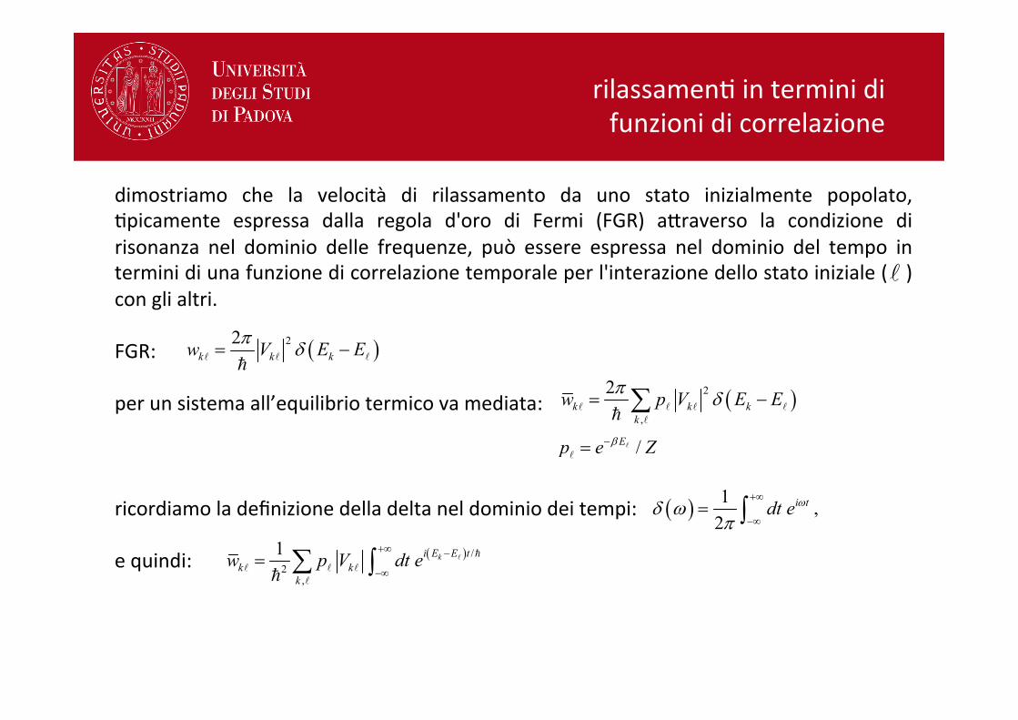
dimostriamo che la velocità di rilassamento da uno stato inizialmente popolato,:picamente espressa dalla regola d'oro di Fermi (FGR) a9raverso la condizione dirisonanza nel dominio delle frequenze, può essere espressa nel dominio del tempo interminidiunafunzionedicorrelazionetemporaleperl'interazionedellostatoiniziale()conglialtri.FGR:perunsistemaall’equilibriotermicovamediata:ricordiamoladefinizionedelladeltaneldominiodeitempi:equindi:

rilassamen:interminidifunzionidicorrelazione

5-13

5.3. RELAXATION RATES FROM CORRELATION FUNCTIONS We have already seen that the rates obtained from first-order perturbation theory are related to

the Fourier transform of the time-dependent external potential evaluated at the energy gap

between the initial and final state. Here we will show that the rate of leaving an initially prepared

state, typically expressed by Fermi’s Golden Rule through a resonance condition in the

frequency domain, can be expressed in the time-domain picture in terms of a time-correlation

function for the interaction of the initial state with others.

The state-to-state form of Fermi’s Golden Rule is

( )22k k kw V E Eπ δ= −A A A=

(5.50)

We will look specifically at the coupling of an initial state A to all other states k. Time-

correlation functions are expressions that apply to systems at thermal equilibrium, so we will

thermally average this expression.

( )2

,

2k k k

k

w p V E Eπ δ= −∑A A A AA=

(5.51)

where /Ep e Zβ−= AA . The energy conservation statement expressed in terms of E or ω can be

converted to the time-domain using the definition of the delta function

( ) 12

i tdt e ωδ ωπ

+∞

−∞= ∫ , (5.52)

giving

( ) /2

,

1 ki E E tk k

k

w p V dt e+∞ −

−∞= ∑ ∫ A =

A A AA=

(5.53)

Writing the matrix elements explicitly and recognizing that 0iH t iE te e= AA A , we have

( ) /2

,

1ki E E t

mnk

w p dt e V k k V+∞ −

−∞= ∑ ∫ A =

AA

A A=

(5.54)

0 02

,

1 iH t iH t

k

p dt V k k e Ve+∞ −

−∞= ∑ ∫A

AA A

= (5.55)

Then, since 1k

k k =∑

( ) ( )2,

1 0mn I Im n

w p dt V t V+∞

−∞=

= ∑ ∫AA

A A=

(5.56)


5-13









(5.50)




( )2

,

2k k k

k


(5.51)



( ) 12

i tdt e ωδ ωπ

+∞

−∞= ∫ , (5.52)

giving

( ) /2

,

1 ki E E tk k

k

w p V dt e+∞ −

−∞= ∑ ∫ A =

A A AA=

(5.53)


( ) /2

,

1ki E E t

mnk


−∞= ∑ ∫ A =

AA

A A=

(5.54)

0 02

,

1 iH t iH t

k


−∞= ∑ ∫A

AA A

= (5.55)

Then, since 1k

k k =∑

( ) ( )2,

1 0mn I Im n

w p dt V t V+∞

−∞=

= ∑ ∫AA

A A=

(5.56)


5-13









(5.50)




( )2

,

2k k k

k


(5.51)



( ) 12

i tdt e ωδ ωπ

+∞

−∞= ∫ , (5.52)

giving

( ) /2

,

1 ki E E tk k

k

w p V dt e+∞ −

−∞= ∑ ∫ A =

A A AA=

(5.53)


( ) /2

,

1ki E E t

mnk


−∞= ∑ ∫ A =

AA

A A=

(5.54)

0 02

,

1 iH t iH t

k


−∞= ∑ ∫A

AA A

= (5.55)

Then, since 1k

k k =∑

( ) ( )2,

1 0mn I Im n

w p dt V t V+∞

−∞=

= ∑ ∫AA

A A=

(5.56)


5-13









(5.50)




( )2

,

2k k k

k


(5.51)



( ) 12

i tdt e ωδ ωπ

+∞

−∞= ∫ , (5.52)

giving

( ) /2

,

1 ki E E tk k

k

w p V dt e+∞ −

−∞= ∑ ∫ A =

A A AA=

(5.53)


( ) /2

,

1ki E E t

mnk


−∞= ∑ ∫ A =

AA

A A=

(5.54)

0 02

,

1 iH t iH t

k


−∞= ∑ ∫A

AA A

= (5.55)

Then, since 1k

k k =∑

( ) ( )2,

1 0mn I Im n

w p dt V t V+∞

−∞=

= ∑ ∫AA

A A=

(5.56)


5-13









(5.50)




( )2

,

2k k k

k


(5.51)



( ) 12

i tdt e ωδ ωπ

+∞

−∞= ∫ , (5.52)

giving

( ) /2

,

1 ki E E tk k

k

w p V dt e+∞ −

−∞= ∑ ∫ A =

A A AA=

(5.53)


( ) /2

,

1ki E E t

mnk


−∞= ∑ ∫ A =

AA

A A=

(5.54)

0 02

,

1 iH t iH t

k


−∞= ∑ ∫A

AA A

= (5.55)

Then, since 1k

k k =∑

( ) ( )2,

1 0mn I Im n

w p dt V t V+∞

−∞=

= ∑ ∫AA

A A=

(5.56)


ℓ

esplicitando,ricordandocheesitrova:

rilassamen:interminidifunzionidicorrelazione

5-13









(5.50)




( )2

,

2k k k

k


(5.51)



( ) 12

i tdt e ωδ ωπ

+∞

−∞= ∫ , (5.52)

giving

( ) /2

,

1 ki E E tk k

k

w p V dt e+∞ −

−∞= ∑ ∫ A =

A A AA=

(5.53)


( ) /2

,

1ki E E t

mnk


−∞= ∑ ∫ A =

AA

A A=

(5.54)

0 02

,

1 iH t iH t

k


−∞= ∑ ∫A

AA A

= (5.55)

Then, since 1k

k k =∑

( ) ( )2,

1 0mn I Im n

w p dt V t V+∞

−∞=

= ∑ ∫AA

A A=

(5.56)


5-13









(5.50)




( )2

,

2k k k

k


(5.51)



( ) 12

i tdt e ωδ ωπ

+∞

−∞= ∫ , (5.52)

giving

( ) /2

,

1 ki E E tk k

k

w p V dt e+∞ −

−∞= ∑ ∫ A =

A A AA=

(5.53)


( ) /2

,

1ki E E t

mnk


−∞= ∑ ∫ A =

AA

A A=

(5.54)

0 02

,

1 iH t iH t

k


−∞= ∑ ∫A

AA A

= (5.55)

Then, since 1k

k k =∑

( ) ( )2,

1 0mn I Im n

w p dt V t V+∞

−∞=

= ∑ ∫AA

A A=

(5.56)


5-13









(5.50)




( )2

,

2k k k

k


(5.51)



( ) 12

i tdt e ωδ ωπ

+∞

−∞= ∫ , (5.52)

giving

( ) /2

,

1 ki E E tk k

k

w p V dt e+∞ −

−∞= ∑ ∫ A =

A A AA=

(5.53)


( ) /2

,

1ki E E t

mnk


−∞= ∑ ∫ A =

AA

A A=

(5.54)

0 02

,

1 iH t iH t

k


−∞= ∑ ∫A

AA A

= (5.55)

Then, since 1k

k k =∑

( ) ( )2,

1 0mn I Im n

w p dt V t V+∞

−∞=

= ∑ ∫AA

A A=

(5.56)


5-13









(5.50)




( )2

,

2k k k

k


(5.51)



( ) 12

i tdt e ωδ ωπ

+∞

−∞= ∫ , (5.52)

giving

( ) /2

,

1 ki E E tk k

k

w p V dt e+∞ −

−∞= ∑ ∫ A =

A A AA=

(5.53)


( ) /2

,

1ki E E t

mnk


−∞= ∑ ∫ A =

AA

A A=

(5.54)

0 02

,

1 iH t iH t

k


−∞= ∑ ∫A

AA A

= (5.55)

Then, since 1k

k k =∑

( ) ( )2,

1 0mn I Im n

w p dt V t V+∞

−∞=

= ∑ ∫AA

A A=

(5.56)


5-14

( ) ( )2

10mn I Iw dt V t V

+∞

−∞= ∫= (5.57)

As before ( ) 0 0iH t iH tIV t e Ve−= . The final expression indicates that integrating over a correlation

function for the time-dependent interaction of the initial state with its surroundings gives the

relaxation or transfer rate. Note that although eq. (5.54) expressed the transfer rate in terms of a

Fourier transform evaluated at the energy gap kE E− A , eq. (5.57) is not a Fourier transform.

processi di rilassamento o trasferimento da uno stato all’altro sipossonoesprimerecomeintegralineltempodifunzionidicorrelazionetemporaledell’interazioneV

funzionidicorrelazioneespe9roscopiaele9ronica

Andrei Tokmakoff, MIT Department of Chemistry, 2/25/2009 6-1

6.1. Time-Correlation Function Description of Absorption Lineshape The interaction of light and matter as we have described from Fermi’s Golden Rule gives the rates

of transitions between discrete eigenstates of the material Hamiltonian H0. The frequency

dependence to the transition rate is proportional to an absorption spectrum. We also know that

interaction with the light field prepares superpositions of the eigenstates of H0, and this leads to the

periodic oscillation of amplitude between the states. Nonetheless, the transition rate expression

really seems to hide any time-dependent description of motions in the system. An alternative

approach to spectroscopy is to recognize that the features in a spectrum are just a frequency

domain representation of the underlying molecular dynamics of molecules. For absorption, the

spectrum encodes the time-dependent changes of the molecular dipole moment for the system,

which in turn depends on the position of electrons and nuclei.

A time-correlation function for the dipole operator can be used to describe the dynamics of

an equilibrium ensemble that dictate an absorption spectrum. We will make use of the transition

rate expressions from first-order perturbation theory that we derived in the previous section to

express the absorption of radiation by dipoles as a correlation function in the dipole operator. Let’s

start with the rate of absorption and stimulated emission between an initial state l and final state

k induced by a monochromatic field

( ) ( )2 202

ˆ2k k kEw kπ ε μ δ ω ω δ ω ω= ⋅ − + +⎡ ⎤⎣ ⎦l l llh

(6.1)

We would like to use this to calculate the experimentally observable absorption coefficient (cross-

section) which describes the transmission through the sample

( )expT N Lα ω= −Δ⎡ ⎤⎣ ⎦ . (6.2)

The absorption cross section describes the rate of energy absorption per unit time relative to the

intensity of light incident on the sample

radEI

α =&

. (6.3)

The incident intensity is

208

cI Eπ

= . (6.4)


















( ) ( )2 202


(6.1)



( )expT N Lα ω= −Δ⎡ ⎤⎣ ⎦ . (6.2)



radEI

α =&

. (6.3)


208

cI Eπ

= . (6.4)


















( ) ( )2 202


(6.1)



( )expT N Lα ω= −Δ⎡ ⎤⎣ ⎦ . (6.2)



radEI

α =&

. (6.3)


208

cI Eπ

= . (6.4)

unapproccioalterna:voallaspe9roscopiaèriconoscerechelecara9eris:chediunospe9rosonolarappresentazioneneldominiodellefrequenzedelladinamicamolecolaredellemolecole,esprimibileconfunzionidicorrelazione.nellaspe9roscopiaele9ronical’osservabilesperimentaleèlaquan:tàdilucetrasmessa/assorbitadalcampione.velocitàdiassorbimentoedemissiones:molata(FGR):chevogliamousarepercalcolarel’osservabilesperimentaletrasmi9anza:

T = II0=10−Abs

⇓leggediLambert-Beer

α =1I0⋅∂E∂t

V = −!µ ⋅!E = −E0 ⋅ ε̂ ⋅

!µ


6-2

If we have two discrete states m and n with m nE E> , the rate of energy absorption is

proportional to the absorption rate and the transition energy

rad nn nmE w ω= ⋅& h . (6.5)

For an ensemble this rate must be scaled by the probability of

occupying the initial state. More generally, we want to consider the

rate of energy loss from the field as a result of the difference in rates

of absorption and stimulated emission between states populated

with a thermal distribution. So, summing all possible initial and

final states l and k over all possible upper and lower states m

and n with m nE E>

( ) ( )

, ,

2 20

, ,

ˆ2

rad k kk m n

k k kk m n

E p w

Ep k

ω

π ω ε μ δ ω ω δ ω ω

=

=

=

= ⋅ − + +⎡ ⎤⎣ ⎦

∑

∑

l l ll

l l l ll

& h

lh

. (6.6)

The cross section including absorption n m→ and stimulated emission m n→ terms is:

( ) ( ) ( )2 2 2

,

4 ˆ ˆmn n mn nm m nmn m

p m n p n mcπα ω ω ε μ δ ω ω ω ε μ δ ω ω⎡ ⎤= ⋅ − + ⋅ +⎢ ⎥⎣ ⎦∑h

(6.7)

To simplify this we note:

1) Since ( ) ( )x xδ δ= − , ( ) ( ) ( )nm mn mnδ ω ω δ ω ω δ ω ω+ = − + = − .

2) The matrix elements squared in the two terms are the same: 2 2

ˆ ˆn m m nε μ ε μ⋅ = ⋅ For

shorthand we will write 2mnμ

3) mn nmω ω= − .

So,

( ) ( ) ( )2

2

,

4mn n m mn mn

n m

p pcπα ω ω μ δ ω ω= − −∑h

(6.8)

Here we see that the absorption coefficient depends on the population difference between the two

states. This is expected since absorption will lead to loss of intensity, whereas stimulated emission

velocitàdellaperditadienergiadelcampocomerisultatodelledifferenzenellevelocitàdiassorbimentoedemissiones:molatatrasta:popola:conunadistribuzionetermica(Boltzmann)Soloduesta::piùsta::ilcoeff.diassorbimento:

6-2



rad nn nmE w ω= ⋅& h . (6.5)







and n with m nE E>

( ) ( )

, ,

2 20

, ,

ˆ2

rad k kk m n

k k kk m n

E p w

Ep k

ω


=

=

=

= ⋅ − + +⎡ ⎤⎣ ⎦

∑

∑

l l ll

l l l ll

& h

lh

. (6.6)


( ) ( ) ( )2 2 2

,



(6.7)






3) mn nmω ω= − .

So,

( ) ( ) ( )2

2

,

4mn n m mn mn

n m


(6.8)



∂Erad

∂t=

6-2



rad nn nmE w ω= ⋅& h . (6.5)







and n with m nE E>

( ) ( )

, ,

2 20

, ,

ˆ2

rad k kk m n

k k kk m n

E p w

Ep k

ω


=

=

=

= ⋅ − + +⎡ ⎤⎣ ⎦

∑

∑

l l ll

l l l ll

& h

lh

. (6.6)


( ) ( ) ( )2 2 2

,



(6.7)






3) mn nmω ω= − .

So,

( ) ( ) ( )2

2

,

4mn n m mn mn

n m


(6.8)



6-2



rad nn nmE w ω= ⋅& h . (6.5)







and n with m nE E>

( ) ( )

, ,

2 20

, ,

ˆ2

rad k kk m n

k k kk m n

E p w

Ep k

ω


=

=

=

= ⋅ − + +⎡ ⎤⎣ ⎦

∑

∑

l l ll

l l l ll

& h

lh

. (6.6)


( ) ( ) ( )2 2 2

,



(6.7)






3) mn nmω ω= − .

So,

( ) ( ) ( )2

2

,

4mn n m mn mn

n m


(6.8)




6-2



rad nn nmE w ω= ⋅& h . (6.5)







and n with m nE E>

( ) ( )

, ,

2 20

, ,

ˆ2

rad k kk m n

k k kk m n

E p w

Ep k

ω


=

=

=

= ⋅ − + +⎡ ⎤⎣ ⎦

∑

∑

l l ll

l l l ll

& h

lh

. (6.6)


( ) ( ) ( )2 2 2

,



(6.7)






3) mn nmω ω= − .

So,

( ) ( ) ( )2

2

,

4mn n m mn mn

n m


(6.8)



ricordandoche:1)2)3)4)siarrivaa:

6-2



rad nn nmE w ω= ⋅& h . (6.5)







and n with m nE E>

( ) ( )

, ,

2 20

, ,

ˆ2

rad k kk m n

k k kk m n

E p w

Ep k

ω


=

=

=

= ⋅ − + +⎡ ⎤⎣ ⎦

∑

∑

l l ll

l l l ll

& h

lh

. (6.6)


( ) ( ) ( )2 2 2

,



(6.7)






3) mn nmω ω= − .

So,

( ) ( ) ( )2

2

,

4mn n m mn mn

n m


(6.8)



= µmn2

6-2



rad nn nmE w ω= ⋅& h . (6.5)







and n with m nE E>

( ) ( )

, ,

2 20

, ,

ˆ2

rad k kk m n

k k kk m n

E p w

Ep k

ω


=

=

=

= ⋅ − + +⎡ ⎤⎣ ⎦

∑

∑

l l ll

l l l ll

& h

lh

. (6.6)


( ) ( ) ( )2 2 2

,



(6.7)






3) mn nmω ω= − .

So,

( ) ( ) ( )2

2

,

4mn n m mn mn

n m


(6.8)



6-3

leads to gain. With equal populations in the upper and lower state, no change to the incident field

would be expected. Since ] /exp[p E Zβ= −l l

[ ]( )1 expn m n mnp p p β ω− = − − h (6.9)

( ) ( ) ( )2

2

,

4 1 n mn mnn m

e pc

β ωπα ω ω μ δ ω ω−= − −∑h

h (6.10)

Note, that the two mnω factors in eq. (6.8) have just been replaced with ω because the delta

function enforces this equality. We can now separate α into a product of factors that represent the

field, and the matter, where the matter is described by ( )σ ω , the absorption lineshape.

( ) ( ) ( )24 1

ce β ωπα ω ω σ ω−= − h

h (6.11)

( ) ( )2

,n mn mn

n mpσ ω μ δ ω ω= −∑ (6.12)

We have already indicated that expressions of the form (6.12) can be expressed as a correlation

function in the operator μ, so following our earlier derivation,

( ) ( ) ( )1 ˆ ˆ02

i tI Idt e tωσ ω ε μ ε μ

π+∞ −

−∞= ⋅ ⋅∫ (6.13)

Here, I added back the light field polarization for a moment. If you assume an isotropic light field,

then you can show that (6.13) can be written as

( ) ( ) ( )1 1 02 3

i tI Idt e tωσ ω μ μ

π+∞ −

−∞= ⋅ ⋅ ∫ (6.14)

or ( ) ( ) ( )1 06 I I

i tdt te ωσ ω μ μπ

+∞

−∞= ∫ (6.15)

The absorption lineshape is given by the Fourier transform of the dipole correlation function. The

correlation function describes the time-dependent behavior or spontaneous fluctuations in the

dipole moment in absence of E field and contains information on states of system and broadening

due to relaxation.

6-3



[ ]( )1 expn m n mnp p p β ω− = − − h (6.9)

( ) ( ) ( )2

2

,

4 1 n mn mnn m

e pc


h (6.10)




( ) ( ) ( )24 1


h (6.11)

( ) ( )2

,n mn mn

n mpσ ω μ δ ω ω= −∑ (6.12)



( ) ( ) ( )1 ˆ ˆ02


π+∞ −

−∞= ⋅ ⋅∫ (6.13)



( ) ( ) ( )1 1 02 3


π+∞ −

−∞= ⋅ ⋅ ∫ (6.14)

or ( ) ( ) ( )1 06 I I


+∞

−∞= ∫ (6.15)




due to relaxation.

6-3



[ ]( )1 expn m n mnp p p β ω− = − − h (6.9)

( ) ( ) ( )2

2

,

4 1 n mn mnn m

e pc


h (6.10)




( ) ( ) ( )24 1


h (6.11)

( ) ( )2

,n mn mn

n mpσ ω μ δ ω ω= −∑ (6.12)



( ) ( ) ( )1 ˆ ˆ02


π+∞ −

−∞= ⋅ ⋅∫ (6.13)



( ) ( ) ( )1 1 02 3


π+∞ −

−∞= ⋅ ⋅ ∫ (6.14)

or ( ) ( ) ( )1 06 I I


+∞

−∞= ∫ (6.15)




due to relaxation.

contributodelsistemamateriale:‘formadibanda’

contributodelcampo

6-2



rad nn nmE w ω= ⋅& h . (6.5)







and n with m nE E>

( ) ( )

, ,

2 20

, ,

ˆ2

rad k kk m n

k k kk m n

E p w

Ep k

ω


=

=

=

= ⋅ − + +⎡ ⎤⎣ ⎦

∑

∑

l l ll

l l l ll

& h

lh

. (6.6)


( ) ( ) ( )2 2 2

,



(6.7)






3) mn nmω ω= − .

So,

( ) ( ) ( )2

2

,

4mn n m mn mn

n m


(6.8)




6-3



[ ]( )1 expn m n mnp p p β ω− = − − h (6.9)

( ) ( ) ( )2

2

,

4 1 n mn mnn m

e pc


h (6.10)




( ) ( ) ( )24 1


h (6.11)

( ) ( )2

,n mn mn

n mpσ ω μ δ ω ω= −∑ (6.12)



( ) ( ) ( )1 ˆ ˆ02


π+∞ −

−∞= ⋅ ⋅∫ (6.13)



( ) ( ) ( )1 1 02 3


π+∞ −

−∞= ⋅ ⋅ ∫ (6.14)

or ( ) ( ) ( )1 06 I I


+∞

−∞= ∫ (6.15)




due to relaxation.

seilcampoèisotropo:

laformadirigadell’assorbimentodipendedallafunzionedicorrelazionetemporaledelmomentodidipolo.

adognifrequenzalospe9rodiassorbimentoèdatodallaFourierTransform(FT)dellafunzione di correlazione del dipolo che descrive le variazioni nel tempo delledistribuzioniele9roniche/nuclearinellemolecoleLa larghezza di banda dipende da come variano queste distribuzioni.Fenomenologicamenteci sonomol:processichecausanotalivariazioni,essipossonoessereclassifica:comeeffe`dinamiciosta:ci.

1  tempodirilassamentodellapopolazione.puòaverecontribu:daprocessiradia:vienon-radia:vi:

poichè,seladifferenzatramednègrandeabbastanza,sololavelocitàversoilbassocontribuisce,edèilmo:vopercuispessoquestocontributosiscrivecome

homogeneousbroadening

6-9

6.3. Ensemble Averaging and Line-Broadening We have seen that an absorption lineshape can represent the dynamics of the dipole or be

broadened by energy relaxation (i.e., coupling to continuum). However, there are numerous

processes that can influence the lineshape. These can be broken into intrinsically molecular and

ensemble average effects. These can be further separated by dynamic processes (homogeneous

broadening) and static effects (inhomogeneous broadening). Let’s review the phenomenological

description. The separation of these effects is a

1. Homogeneous broadening

Several homogeneous (dynamic) line broadening mechanisms are possible, which are qualitatively

captured by a time-scale 2T . If these processes are independent, the exponential rates for different

contributions add:

*2 1 2

1 1 1 1

orT T T τ= + + (6.45)

a. Molecular processes

Population Relaxation. Population relaxation 1T refers to amplitude decay in the

coherent superposition created by the light field as a result of it finite lifetime. This can

have contributions from radiative decay (spontaneous emission processes) or non-

radiative processes (i.e., coupling to continuum and IVR)

1

1 1 1

rad NRT τ τ= + (6.46)

In this case, ensemble averaging doesn’t change the measurement. All members of

ensemble behave identically and the experimentally measured decay is the microscopic

lifetime.

The observed population relaxation time depends on both the relaxation times of the

upper and lower states (m and n) being coupled by the field: 11 mn nmT w w= + . When the

energy splitting is high, only the downward rate contributes, which is why the rate is often

written 11 2T .

6-9










contributions add:

*2 1 2

1 1 1 1

orT T T τ= + + (6.45)






1

1 1 1

rad NRT τ τ= + (6.46)



lifetime.




written 11 2T .

6-9










contributions add:

*2 1 2

1 1 1 1

orT T T τ= + + (6.45)






1

1 1 1

rad NRT τ τ= + (6.46)



lifetime.




written 11 2T .

meccanismidinamicica9ura:fenomenologicamentedaT2:

6-9










contributions add:

*2 1 2

1 1 1 1

orT T T τ= + + (6.45)






1

1 1 1

rad NRT τ τ= + (6.46)



lifetime.




written 11 2T .

1 2 3

2puredephasing:randomizzazionedella fase inunensembledimolecoleacausadiinterazioniinter-molecolari

3 orientazione delle molecole che cambia nel tempo: randomizzazionedell’orientazioneinizialedelmomentodidipolo

puredephasing

6-10

b. Ensemble processes

Pure Dephasing. Pure dephasing is characterized by a time constant *2T that

characterizes the randomization of phase within an ensemble as a result of molecular

interactions. This is a dynamic ensemble averaging effect in which the phase relationship

of oscillation between members of the ensemble is gradually destroyed. Examples include

collisions in a dense gas, or fluctuations induced by a solvent.

Orientational relaxation ( )orτ also leads to relaxation of the dipole correlation function

and to line broadening. Since the correlation function depends on the projection of the

dipole onto a fixed axis in the laboratory frame, randomization of the initial dipole

orientations is an ensemble averaged dephasing effect. In solution, this process is

commonly treated as an orientational diffusion problem in which orτ is proportional to

the diffusion constant.

2. Inhomogeneous Broadening

Absorption lineshapes can also be broadened by a static distribution of frequencies. If molecules

within the ensemble are influenced static environmental variations more than other processes,

then the observed lineshape reports on the distribution of environments. This inhomogeneous

inhomogeneousbroadening

dovutoadistribuzionesta:cadellefrequenze,quan:ficatadaΔ,larghezzadelladistribuzione.

6-11

broadening is a static ensemble averaging effect, which hides the dynamical content in the

homogeneous linewidth. The origin of the inhomogeneous broadening can be molecular (for

instance a distribution of defects in crystals) or macroscopic (i.e. an inhomogeneous magnetic

field in NMR).

The inhomogeneous linewidth is dictated the width of the distribution Δ. Total Linewidth The total observed broadening of the absorption lineshape reflects the contribution of all of these

effects:

( ) ( ) 2 2 /2*

2 1

1 1 10 exp

2t

or

t tT T

eμ μτ

−Δ⎡ ⎤⎛ ⎞∝ − + +⎢ ⎥⎜ ⎟

⎝ ⎠⎣ ⎦ (6.47)

These effects can be wrapped into a lineshape function g(t). The lineshape for the broadening of

a given transition can be written as the Fourier transform over the oscillating transition frequency

damped and modulated by a complex g(t):

( ) ( )12

mni t g ti tdt e e ωωσ ωπ

+∞ −−

−∞= ∫ (6.48)

All of these effects can be present simultaneously in an absorption spectrum.

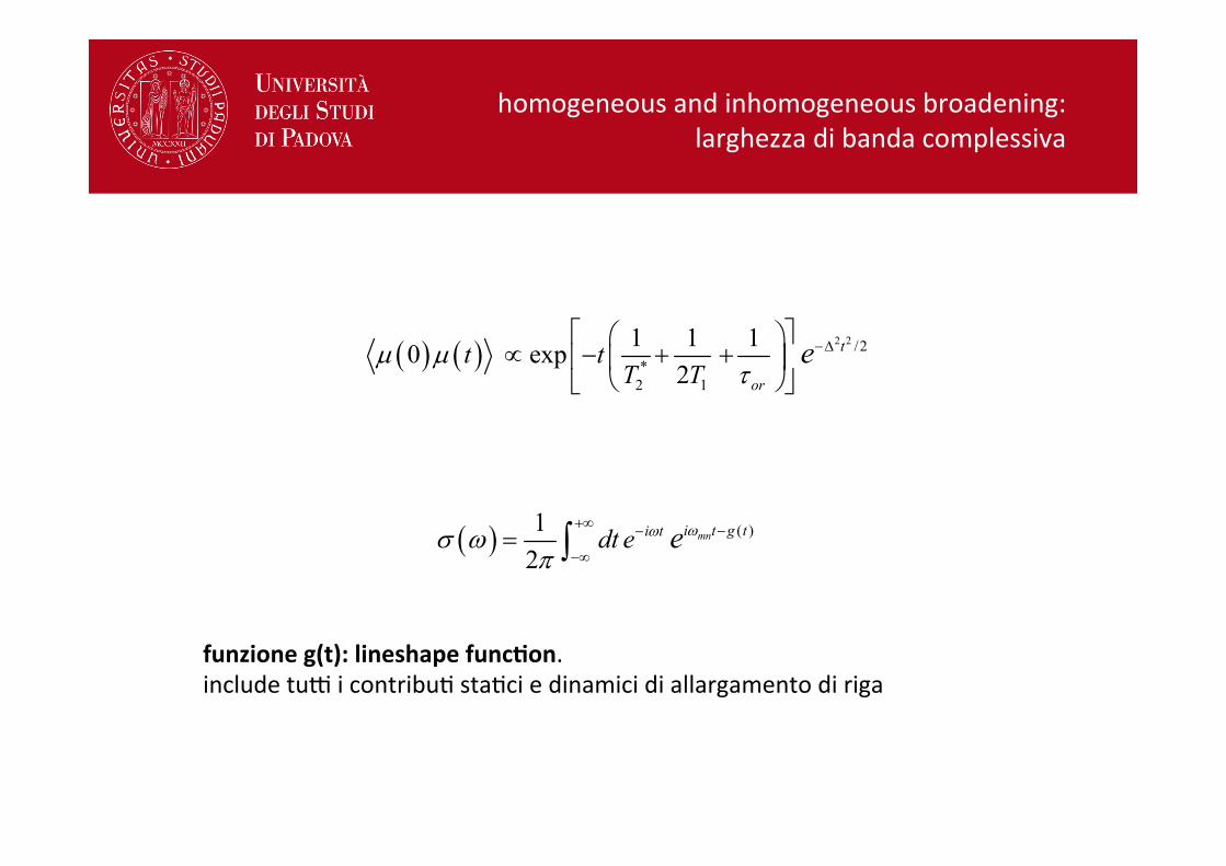
homogeneousandinhomogeneousbroadening:larghezzadibandacomplessiva

6-11




field in NMR).


effects:

( ) ( ) 2 2 /2*

2 1

1 1 10 exp

2t

or

t tT T

eμ μτ

−Δ⎡ ⎤⎛ ⎞∝ − + +⎢ ⎥⎜ ⎟

⎝ ⎠⎣ ⎦ (6.47)




( ) ( )12


+∞ −−

−∞= ∫ (6.48)


6-11




field in NMR).


effects:

( ) ( ) 2 2 /2*

2 1

1 1 10 exp

2t

or

t tT T

eμ μτ

−Δ⎡ ⎤⎛ ⎞∝ − + +⎢ ⎥⎜ ⎟

⎝ ⎠⎣ ⎦ (6.47)




( ) ( )12


+∞ −−

−∞= ∫ (6.48)


funzioneg(t):lineshapefunc6on.includetu`icontribu:sta:ciedinamicidiallargamentodiriga

funzioni di correlazione - unipd.it di correlazione... · funzioni di correlazione in generale si...

Documents