fundamentals of the split hopkinson pressure bar - iul · an impact produces compressive waves...

1

Dr.-Ing. Erhardt Lach

French-German Research Institute of Saint-Louis, ISL

[email protected]

High Dynamic Testing of Materials

Fundamentals of the Split Hopkinson pressure bar

E. Lach 2

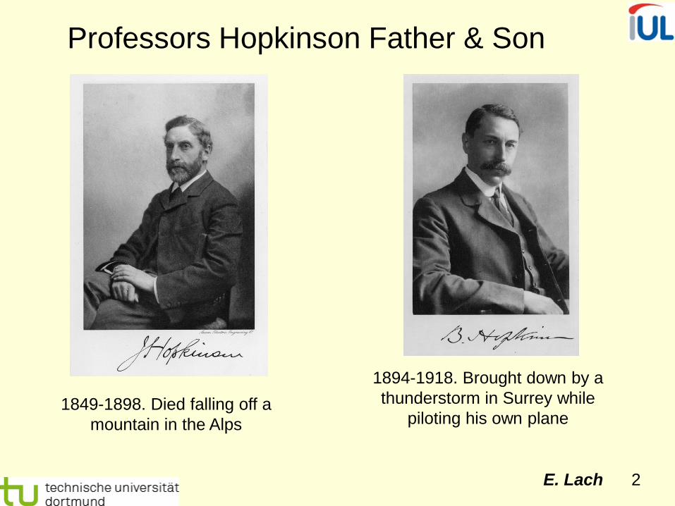
Professors Hopkinson Father & Son

1849-1898. Died falling off a mountain in the Alps

1894-1918. Brought down by a thunderstorm in Surrey while

piloting his own plane

E. Lach 3

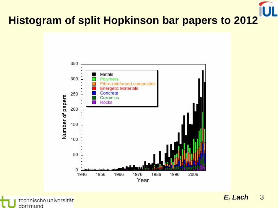
Histogram of split Hopkinson bar papers to 2012

E. Lach 4

specimen

counter

amplifier

PC A/D

light barrier

compressed air

photodiode

gas gun

gauge I gauge II

incident bar

transmission bar

pneumatic control system

projectile

printer

Classical Split Hopkinson Pressure Bar

E. Lach 5

E. Lach 6

Generally, the loading method can be static or dynamic.

Static load type of SHPB

The section of the incident bar between the far end from the specimen and a clamp is statically loaded in compression. The energy stored due to such precompression is released into the initially unstressed section of the incident bar when the clamp is suddenly released. This produces a compression wave propagating in the incident bar towards the specimen.

Asprone, D., Cadoni, E., Prota, A., Manfredi, G. (2009). ”Strain-Rate Sensitivity of a Pultruded E-Glass/Polyester Composite.” J. Compos. Constr., 13(6), 558–564.

E. Lach 7

Schematic presentation of a SHPB test

E. Lach 8

An impact produces compressive waves propagating (c0) into projectile and bar. At the end of the projectile the compressive wave reflects back as a release wave. This determines the length of the wave (Λ=2L).

M. A. Meyers, Dynamic Behavior of Materials, Wiley, New York, 1994

E. Lach 9

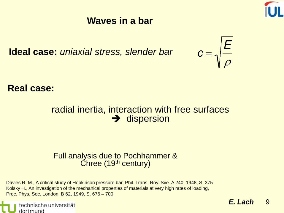
Ideal case: uniaxial stress, slender bar

Waves in a bar

Real case:

radial inertia, interaction with free surfaces dispersion

Full analysis due to Pochhammer & Chree (19th century)

Davies R. M., A critical study of Hopkinson pressure bar, Phil. Trans. Roy. Sve. A 240, 1948, S. 375 Kolsky H., An investigation of the mechanical properties of materials at very high rates of loading, Proc. Phys. Soc. London, B 62, 1949, S. 676 – 700

E. Lach 10

f(t) = + Σ Dn cos (nω0 t – δn) A0

2 ∞

n = 1

At any position, z, along the pressure bar, the wave, f(t), may be presented by an infinite cosine Fourier series:

ω0 is the frequency of the longest wave length (n=1), δn is the phase angle of component n ω0 .

Kolsky H., An investigation of the mechanical properties of materials at very high rates of loading, Proc. Phys. Soc. London, B 62, 1949, S. 676 – 700

E. Lach 11

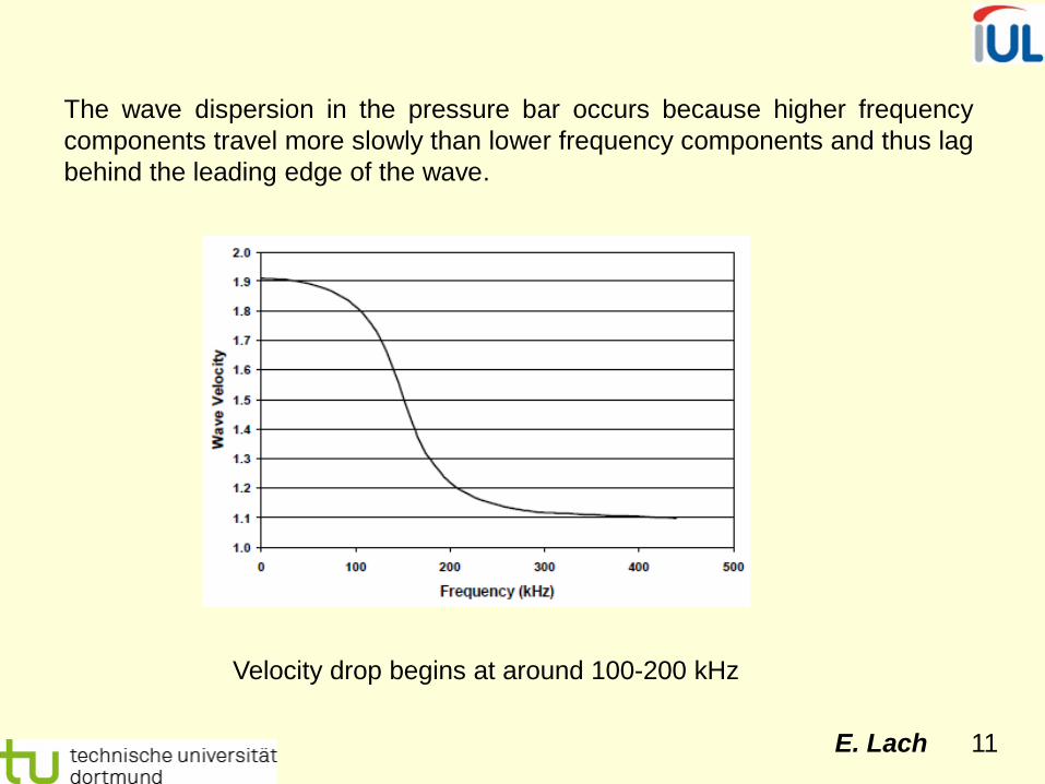
Velocity drop begins at around 100-200 kHz

The wave dispersion in the pressure bar occurs because higher frequency components travel more slowly than lower frequency components and thus lag behind the leading edge of the wave.

E. Lach 12

1D stress wave propagation assumed Not valid for low wavelengths

(where λ approaches d)

Equation for solid cylinder derived by Pochhammer (contemporaneously by Chree):

Pochhammer L., Journal Reine und Angewandte Mathematik 81, 1876, S. 324 Chree C., Trans. Camb. Phil. Soc., 14, 1889, S. 250

E. Lach 13

In the Pochhammer-Chree’s longitudinal wave analysis, it is assumed that the wave is harmonic as follows

( ) ( ) ( )[ ] ωωπ

ωωξ derutzru tzi −+∞

∞−∫= ,

21,,,

where u(r,z,t) is the displacement vector.

E. Lach 14

uK = FK exp[i 2π/λ (z + c0 ∙ t)] (K = r, θ, z)

77777wjsn

uz R

ur

Uθ

ur = u (r, θ) exp[i 2π/λ (z + c0 ∙ t)]

uθ = v (r, θ) exp[i 2π/λ (z + c0 ∙ t)] uz = w (r, θ) exp[i 2p/λ (z + c0 ∙ t)]

Love summarized the theory of Pochhammer. The solution in cylindrical polar coordinates is, in the general spelling, like follows:

Where u, v and w are only a function of r and θ.


E. Lach 15

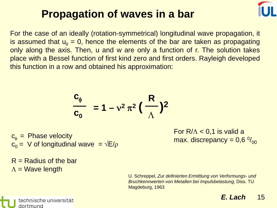
cφ

c0 = 1 – ν2 π2 ( )2

R

Λ

cφ = Phase velocity c0 = V of longitudinal wave = √E/ρ R = Radius of the bar Λ = Wave length

Propagation of waves in a bar For the case of an ideally (rotation-symmetrical) longitudinal wave propagation, it is assumed that uθ = 0, hence the elements of the bar are taken as propagating only along the axis. Then, u and w are only a function of r. The solution takes place with a Bessel function of first kind zero and first orders. Rayleigh developed this function in a row and obtained his approximation:

For R/Λ < 0,1 is valid a max. discrepancy = 0,6 0/00

U. Schreppel, Zur definierten Ermittlung von Verformungs- und Bruchkennwerten von Metallen bei Impulsbelastung, Diss. TU Magdeburg, 1963

E. Lach 16

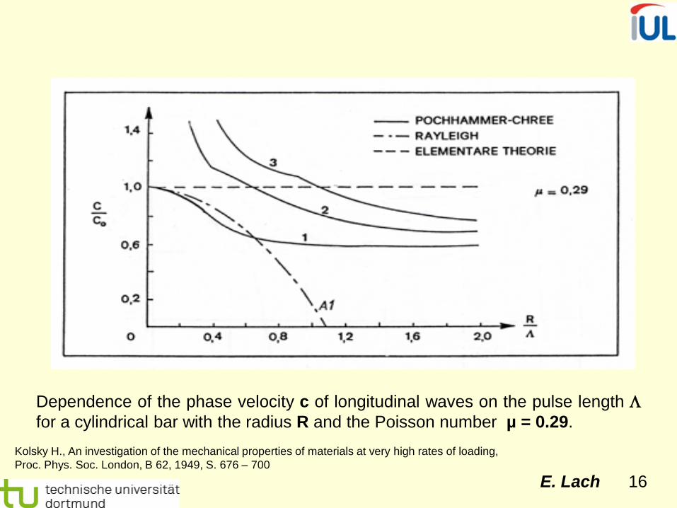
Dependence of the phase velocity c of longitudinal waves on the pulse length Λ for a cylindrical bar with the radius R and the Poisson number µ = 0.29.


E. Lach 17

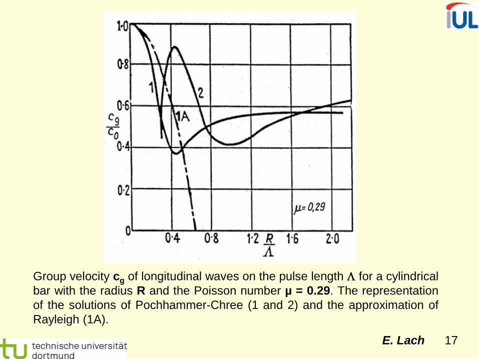
Group velocity cg of longitudinal waves on the pulse length Λ for a cylindrical bar with the radius R and the Poisson number µ = 0.29. The representation of the solutions of Pochhammer-Chree (1 and 2) and the approximation of Rayleigh (1A).

E. Lach 18

The energy transportation through a rod is dependent, in the real case (with dispersion), on the group velocity of all occurring wavelengths and not only on the phase speed c: cg = c - Λ dc / dΛ The dependence of R/Λ on cg/c is illustrated in slide 17. Fig. 16 shows that the curves 2 and 3 can assume values greater than 1. From this follows that the phase velocity can become larger than c0. That is not possible for the group velocity. The highest velocity in a finite bar is c0. Slide 17 shows that the solution is applicable to smaller values of R/Λ after Rayleigh, as it was represented in slide 17 for c/c0. Curve 1 in slide 17 (cg/c0) shows an approximate minimum of R/Λ = 0.45. In contrast to this, curve 2 has its maximum here.


E. Lach 19

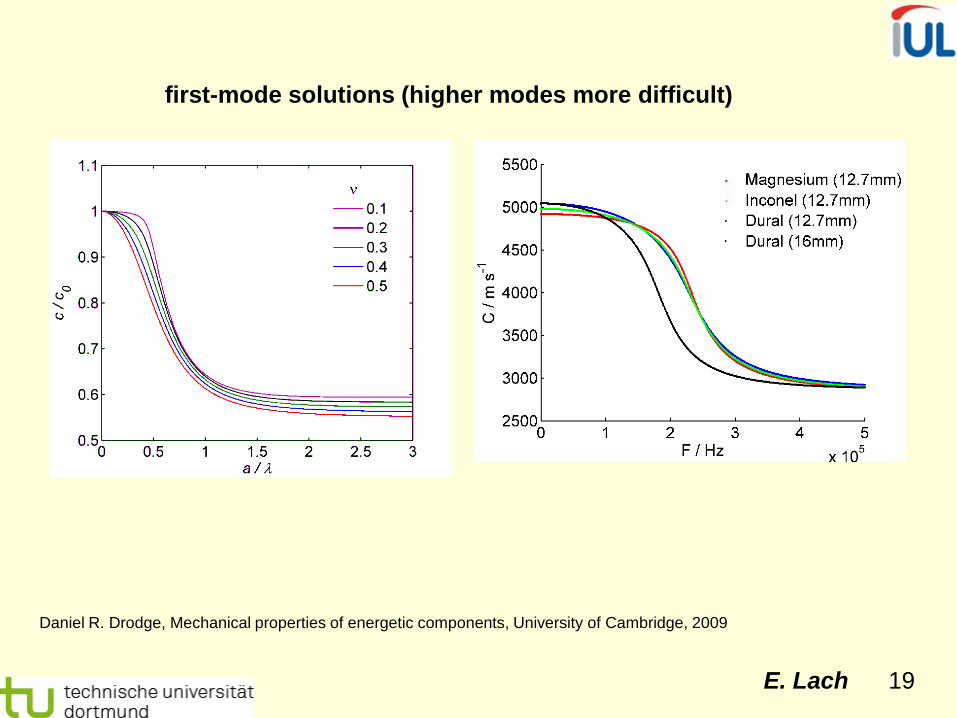
first-mode solutions (higher modes more difficult)

Daniel R. Drodge, Mechanical properties of energetic components, University of Cambridge, 2009

E. Lach 20

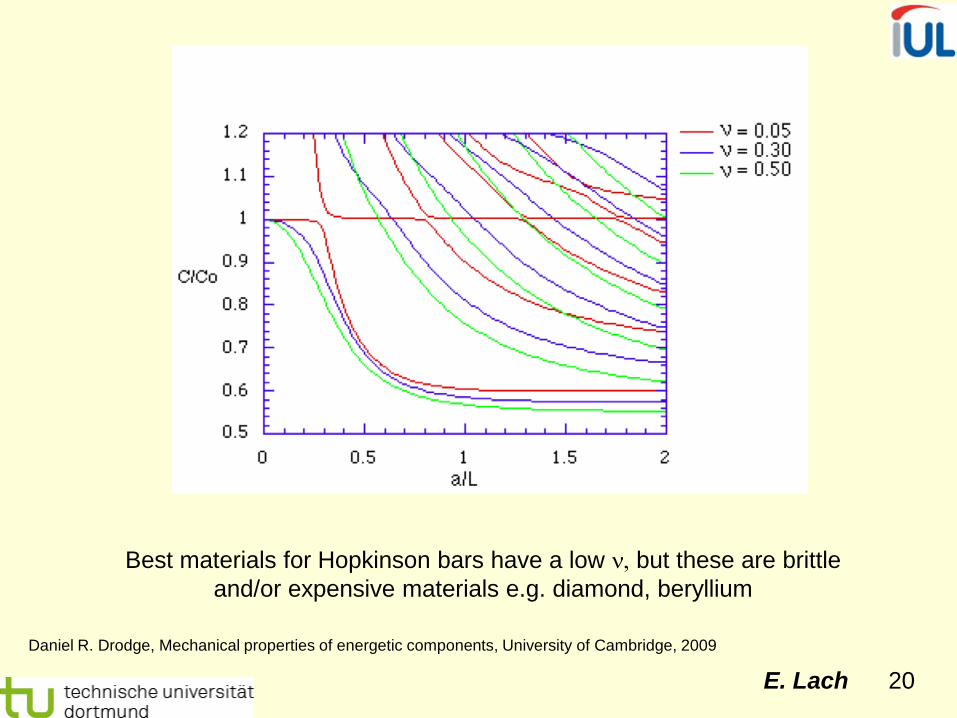
Best materials for Hopkinson bars have a low ν, but these are brittle and/or expensive materials e.g. diamond, beryllium


E. Lach 21

u z

rri

Brepta R., Acta technica ČSAV, 1968, p.770

E. Lach 22

Assumptions

• Elastic wave propagation follos mono-dimensional theory (non dispersive)

• Uniaxial stress distribution

• Friction between bars and specimen is neglected

• Radial and axial inertia is neglected

E. Lach 23

S.T. Marais et al, Material testing at high strain rate using the split Hopkinson pressure bar, Latin American Journal of Solids and Structures, 1 (2004), p. 319 - 339

E. Lach 24

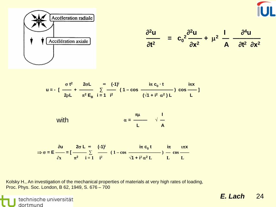
∂2u ∂2u I ∂4u —— = c0

2 —— + µ2 — ———— ∂t2 ∂x2 A ∂t2 ∂x2

σ t2 2σL ∞ (-1)i iπ c0 ∙ t iπx u = - [ —— + ——— ∑ —— ( 1 – cos ——————— ) cos —— ] 2ρL π2 EB i = 1 i2 (√1 + i2 α2 ) L L

πµ I α = ——— √ — L A

with

∂u 2σ L ∞ (-1)i iπ c0 t iπ ιπx ⇒ σ = E —— = [ ——— ∑ —— ( 1 – cos ——————— ) — cos —— ∂x π2 i = 1 i2 √1 + i2 α2 L L L


E. Lach 25

E. Lach 26

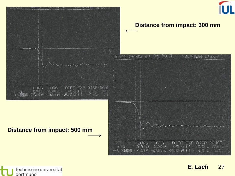
Extent of P-C “oscillations” also decreases with initial rise time

Pulse rise time is thus important


E. Lach 27

Distance from impact: 300 mm


E. Lach 28


E. Lach 29

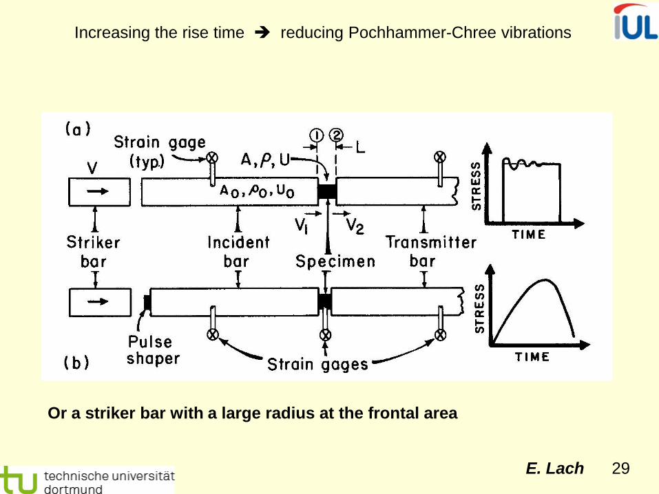
Or a striker bar with a large radius at the frontal area

Increasing the rise time reducing Pochhammer-Chree vibrations

E. Lach 30

3-bar SHPB

Modified SHPB system for pulse shaping

Specimen strain and strain rate variation; A, no pulse shaping, mean strain rate 1900 s-1; B, with pulse shaping, mean strain rate 1800 s-1.

Ellwood S., Griffiths L.J., Parry D.J., Materials testing at high constant strain rates, J. Phys. E: Sci. Instrum., Vol. 15, 1982, p. 280-282

E. Lach 31

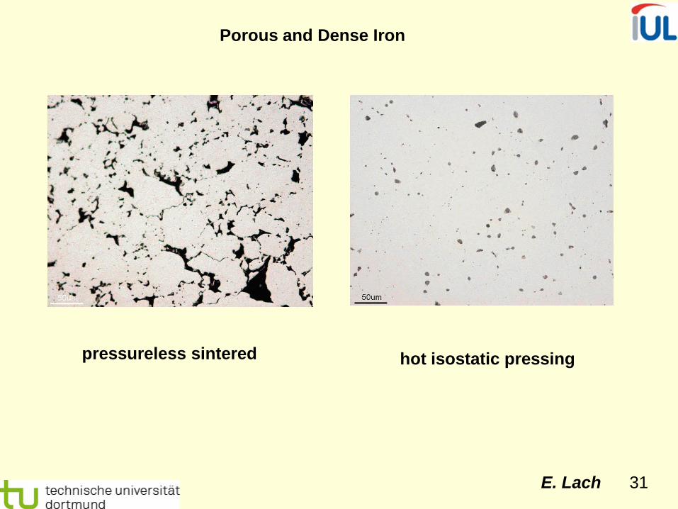
Porous and Dense Iron

pressureless sintered hot isostatic pressing

E. Lach 32

0

200

400

600

800

1000

0 0.1 0.2 0.3 0.4 0.5

True

Str

ess

True Strain

MPa

sintered

hot-isostatic pressed

E. Lach 33

-0.3-0.2-0.1

00.10.20.30.40.5

80 280 480 680 880

VOLT

AGE,

V

TIME, µs

-0.04

0

0.04

0.08

0.12

0.16

0.2

500 600 700 800 900

VOLT

AGE,

V

TIME, µs

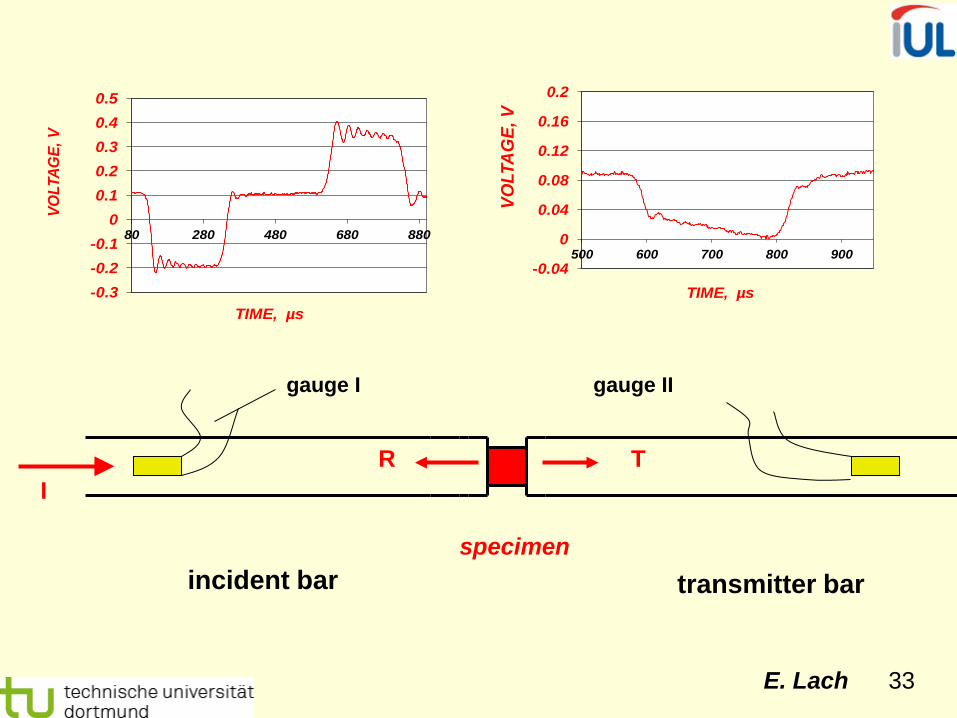
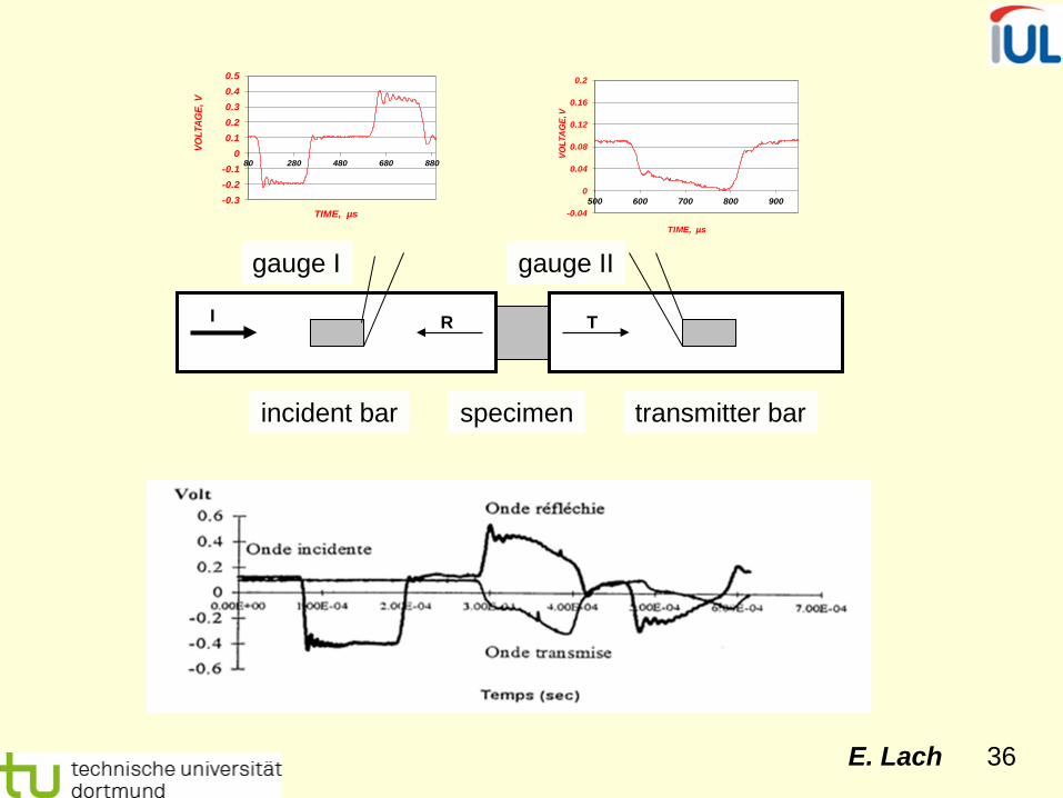
incident bar transmitter bar

gauge I

specimen

I R T

gauge II

E. Lach 34

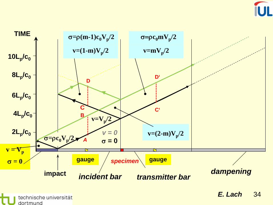
gauge v = Vp

v=Vp/2

σ=ρ(m-1)c0Vp/2

impact

10Lp/c0

8Lp/c0

6Lp/c0

4Lp/c0

2Lp/c0 v = 0 σ = 0 σ=ρc0Vp/2

v=(2-m)Vp/2

D‘

C‘

D

C B

A

specimen

transmitter bar dampening

TIME σ=ρc0mVp/2

v=mVp/2 v=(1-m)Vp/2

σ = 0 gauge

incident bar

E. Lach 35

-0.3-0.2-0.1

00.10.20.30.40.5

560 660 760 860VO

LTA

GE,

V

TIME, µs -0.04

0

0.04

0.08

0.12

0.16

0.2

500 600 700 800 900

VOLT

AG

E, V

TIME, µs

specimen gauge I gauge II

incident bar transmitter bar

E. Lach 36

I R T

Eingangsstab Ausgangsstab Probe

DMS I DMS II

-0.3-0.2-0.1

00.10.20.30.40.5

80 280 480 680 880

VOLT

AGE,

VTIME, µs -0.04

0

0.04

0.08

0.12

0.16

0.2

500 600 700 800 900

VOLT

AG

E, V

TIME, µs

gauge II gauge I

specimen transmitter bar incident bar

E. Lach 37

σI = σR + σT

E. Lach 38

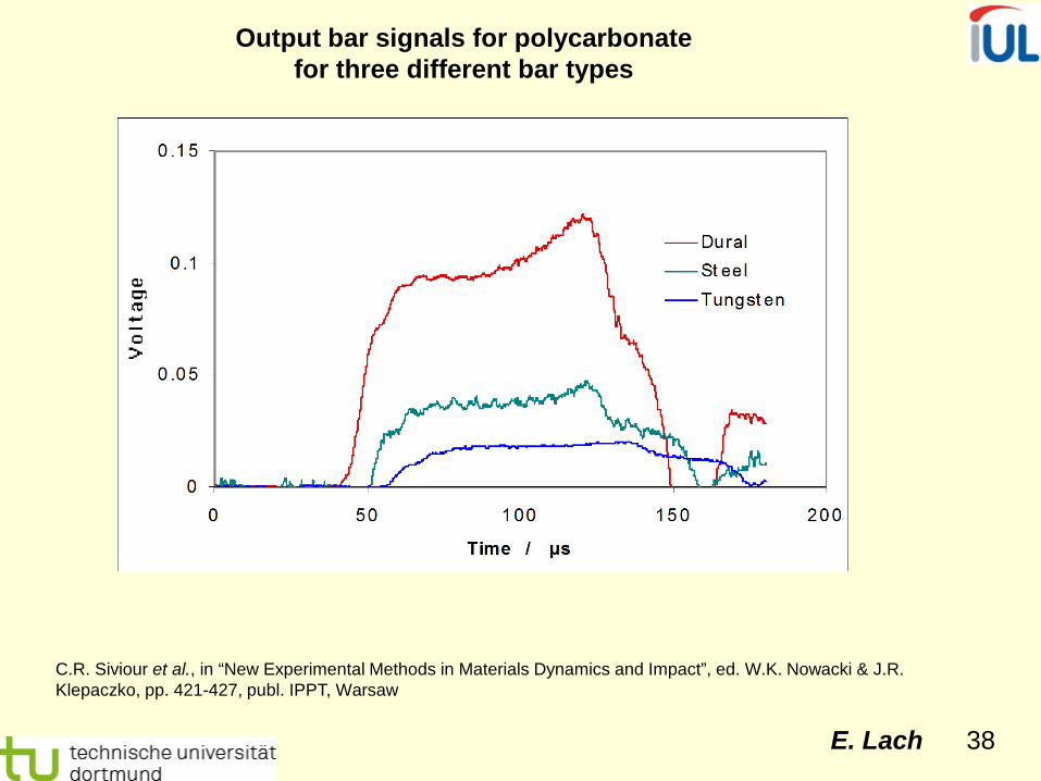
Output bar signals for polycarbonate for three different bar types

C.R. Siviour et al., in “New Experimental Methods in Materials Dynamics and Impact”, ed. W.K. Nowacki & J.R. Klepaczko, pp. 421-427, publ. IPPT, Warsaw

E. Lach 39

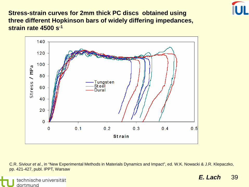
Stress-strain curves for 2mm thick PC discs obtained using three different Hopkinson bars of widely differing impedances, strain rate 4500 s-1

C.R. Siviour et al., in “New Experimental Methods in Materials Dynamics and Impact”, ed. W.K. Nowacki & J.R. Klepaczko, pp. 421-427, publ. IPPT, Warsaw

E. Lach 40

G. T. Gray III, High-Strain-Rate Testing of Materials: The Split Hopkinson Pressure Bar, Methods in Materials Research, E. Kaufmann, Ed., Wiley, 1999

E. Lach 41

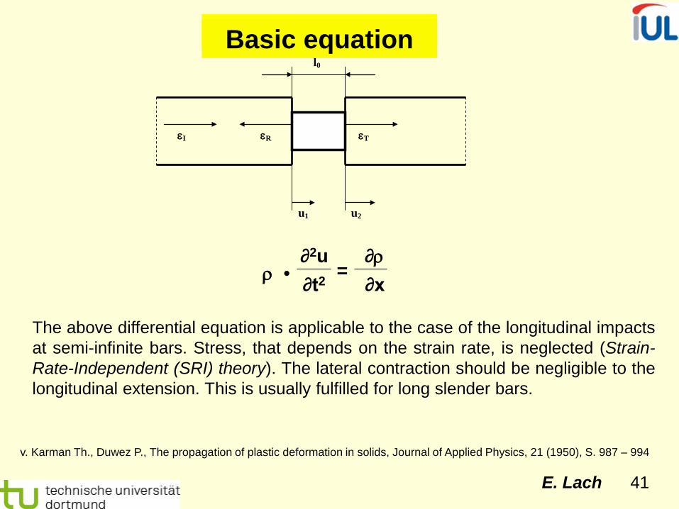
Grundgleichungen

∂2u ∂ρ ρ • =

∂t2 ∂x

The above differential equation is applicable to the case of the longitudinal impacts at semi-infinite bars. Stress, that depends on the strain rate, is neglected (Strain-Rate-Independent (SRI) theory). The lateral contraction should be negligible to the longitudinal extension. This is usually fulfilled for long slender bars.

v. Karman Th., Duwez P., The propagation of plastic deformation in solids, Journal of Applied Physics, 21 (1950), S. 987 – 994

l0

u1 u2

εI εR εT

Basic equation

E. Lach 42

Hook’s law is applicable to the case of the purely elastic mechanical loading (bars of the Hopkinson bar):

∂u σ = —— • E

∂x

Young‘s modulus E is related to the velocity c0 of a longitudinal elastic wave and the density ρ according to equation c0 = √E / ρ.

∂2u ∂2u —— = c02 ——

∂t2 ∂x2

The general solution of this simplified wave equation is:

u (x, t) = g(x - c0• t) + f(x + c0 • t)

If the wave propagates only in a positive direction, the following equation is valid:

u |x, t| = f |x + c0 • t|

E. Lach 43

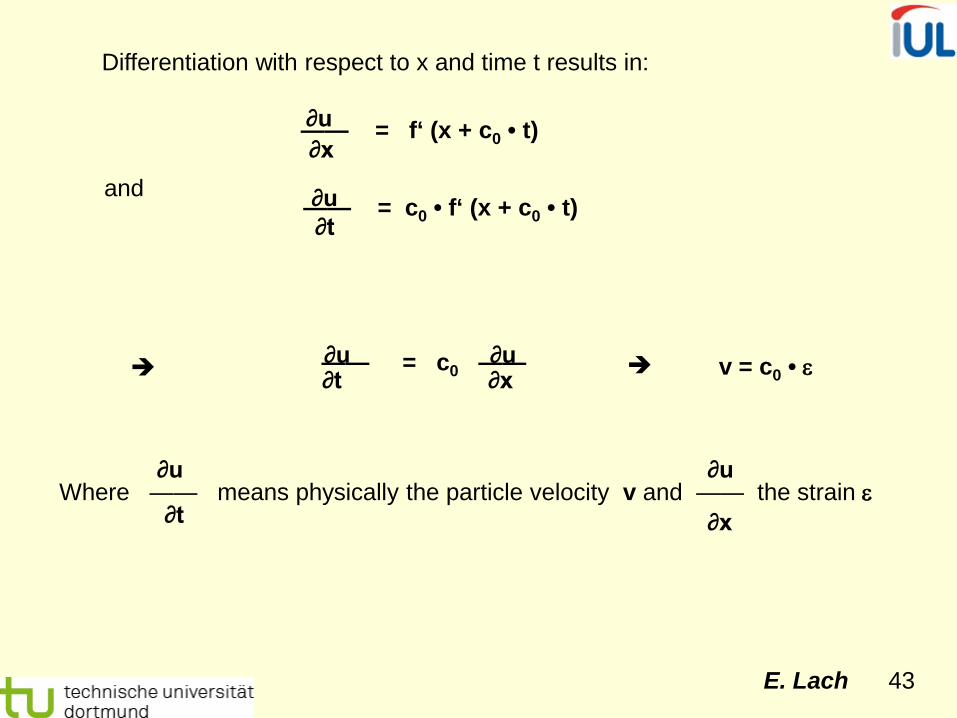
Differentiation with respect to x and time t results in:

∂u —— = f‘ (x + c0 • t) ∂x and ∂u —— = c0 • f‘ (x + c0 • t) ∂t

∂u ∂u —— = c0 —— ∂t ∂x v = c0 • ε

Where —— means physically the particle velocity v and —— the strain ε ∂u ∂u

∂t ∂x

E. Lach 44

and

result in

E. Lach 45

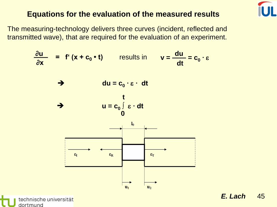
Equations for the evaluation of the measured results

The measuring-technology delivers three curves (incident, reflected and transmitted wave), that are required for the evaluation of an experiment.

results in v = —— = c0 ∙ ε du dt

du = c0 ∙ ε ∙ dt

u = c0 ∫ ε ∙ dt t

0

E. Lach 46

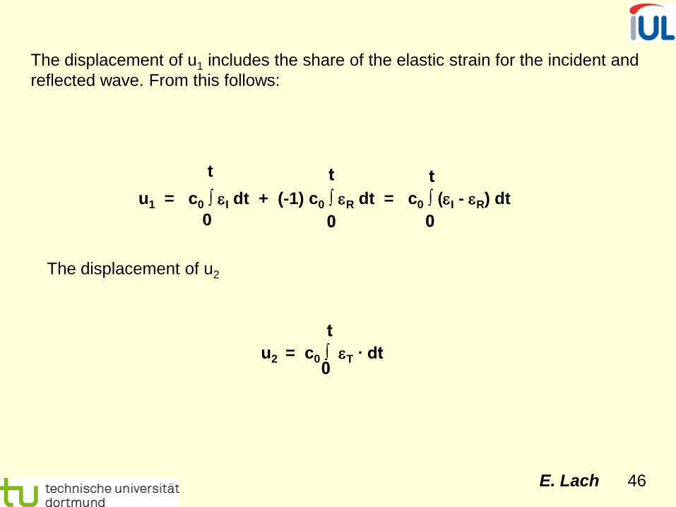
The displacement of u1 includes the share of the elastic strain for the incident and reflected wave. From this follows:

u1 = c0 ∫ εI dt + (-1) c0 ∫ εR dt = c0 ∫ (εI - εR) dt t

0

The displacement of u2

u2 = c0 ∫ εT ∙ dt

E. Lach 47

The mean strain of a specimen can be calculated from both displacements:

εS = ———— = —— ∫ (εI - εR - εT ) dt _ u1 - u2

L0

c0

L0

t

0

These expressions can be simplified under the assumption that the stress remains constant within the specimen. This is the case with adequately small specimen (L0 → 0) and the following is valid:

εR = εI - εT

εS = - ——— ∫ εR dt _ 2c0

L0 0

t

E. Lach 48

The mean strain rate results in the following equation:

εS = ——— = ——— εR dε _

dt

2c0

L0

Calculate the stresses, the following balance of forces is drawn up:

P1 = EBA (εI + εR)

and P2 = EBA εT

E. Lach 49

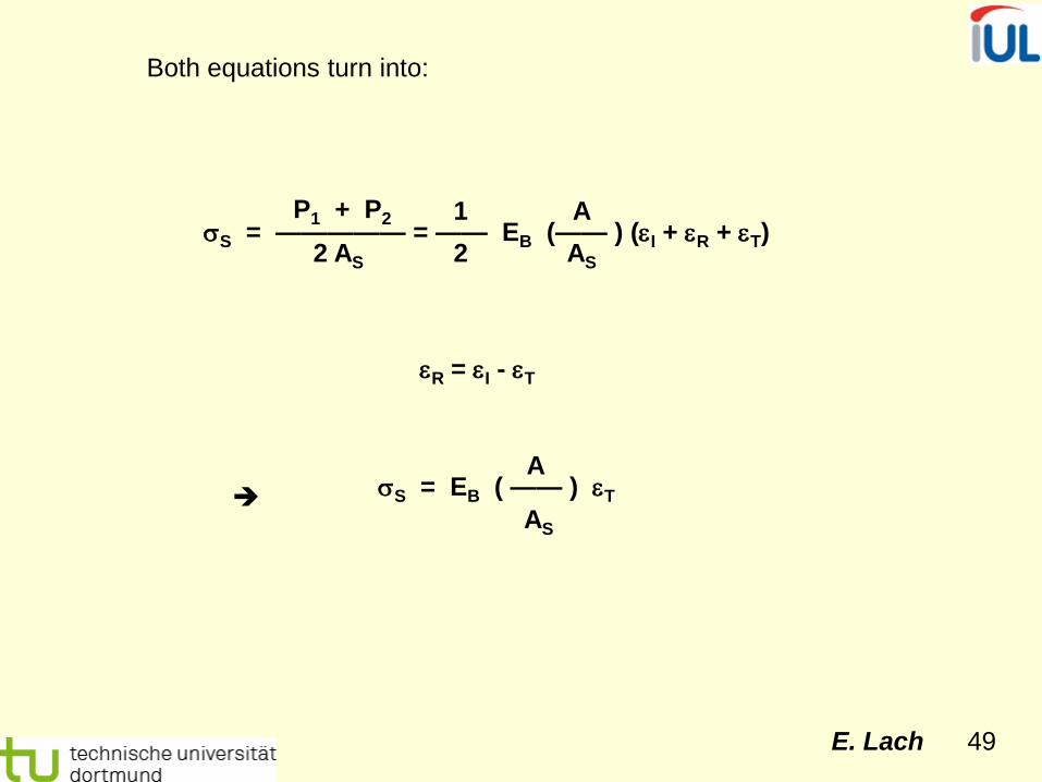
Both equations turn into:

σS = ————— = —— EB (—— ) (εI + εR + εT) P1 + P2

2 AS 1 2

A AS

εR = εI - εT

σS = EB ( —— ) εT A

AS

E. Lach 50

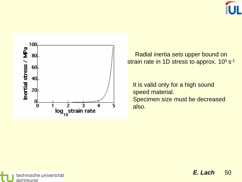
Radial inertia sets upper bound on strain rate in 1D stress to approx. 105 s-1

It is valid only for a high sound speed material. Specimen size must be decreased also.

E. Lach 51

( ) 222

022

0021 16128122

1 εµερσσσ

−−

+−+−=

alal

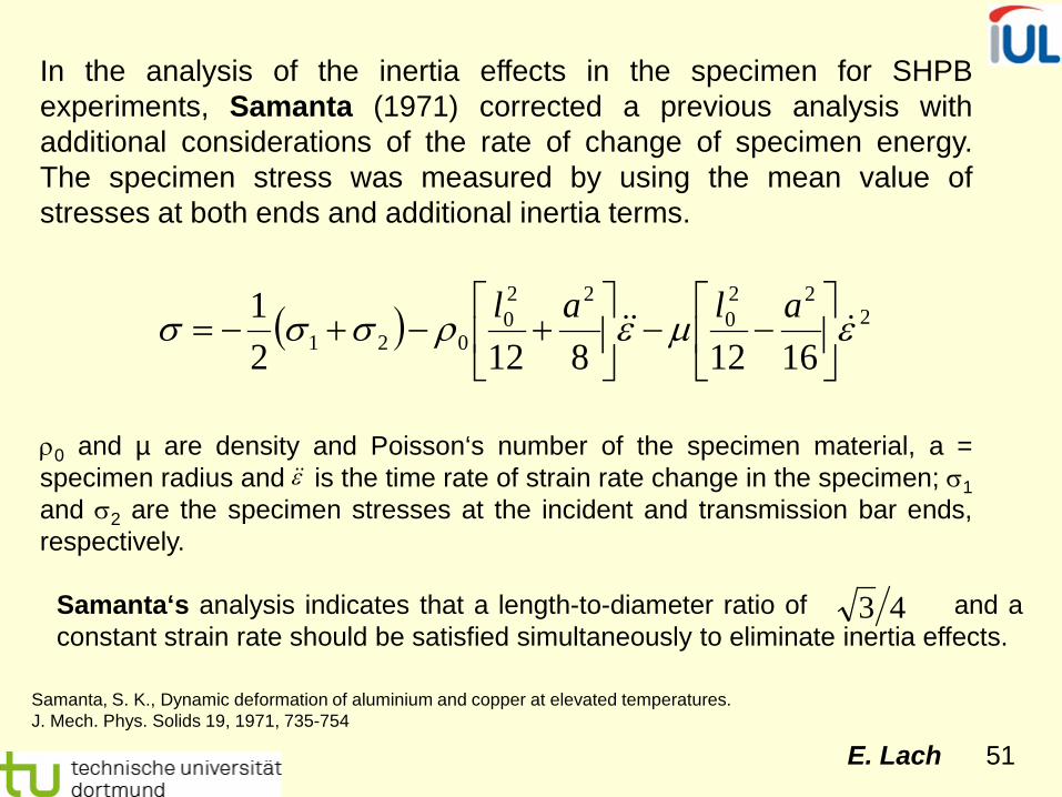
In the analysis of the inertia effects in the specimen for SHPB experiments, Samanta (1971) corrected a previous analysis with additional considerations of the rate of change of specimen energy. The specimen stress was measured by using the mean value of stresses at both ends and additional inertia terms.

ρ0 and µ are density and Poisson‘s number of the specimen material, a = specimen radius and is the time rate of strain rate change in the specimen; σ1 and σ2 are the specimen stresses at the incident and transmission bar ends, respectively.

ε

Samanta‘s analysis indicates that a length-to-diameter ratio of and a constant strain rate should be satisfied simultaneously to eliminate inertia effects.

43

Samanta, S. K., Dynamic deformation of aluminium and copper at elevated temperatures. J. Mech. Phys. Solids 19, 1971, 735-754

E. Lach 52

Inertia effects in specimen Inertia effects are associated with most dynamic events. In a SHPB the specimen is initially at rest and expected to deform at a desired rate. The deformation at high rates is accompanied by inertia in both axial and radial direction due to acceleration. Inertia effects should be minimized through appropriate design of specimen geometry and experimental conditions in order to avoid failure in the measured signals.

σ (t) = σm (t) + ρs │ ── - µs ── │ ──── ls2

6 d2

8 ∂2 ε (t)

∂t2

┌

└

┐

┘

── = ─── ls d

3 µs

4 ls/d – aspect ratio relating to minimal inertia

effects 0.5

Bertholf I. D., Karnes C. H., 2D analysis of the split Hopkinson pressure bar system, J. Mech. Phys. Solids, 23, 1975, S. 1 – 19

In the equation, σm mean the measured stress, µ the Poisson number, ls the length and d the diameter of the specimen, ρ the density of the specimen

E. Lach 53

E. Lach 54

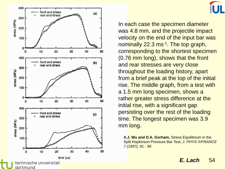
In each case the specimen diameter was 4.8 mm, and the projectile impact velocity on the end of the input bar was nominally 22.3 ms-1. The top graph, corresponding to the shortest specimen (0.76 mm long), shows that the front and rear stresses are very close throughout the loading history, apart from a brief peak at the top of the initial rise. The middle graph, from a test with a 1.5 mm long specimen, shows a rather greater stress difference at the initial rise, with a significant gap persisting over the rest of the loading time. The longest specimen was 3.9 mm long.

X.J. Wu and D.A. Gorham, Stress Equilibrium in the Split Hopkinson Pressure Bar Test, J. PHYS IVFRANCE 7 (1997), 91 - 96

E. Lach 55

Comparison of stresses at front and rear ends of a 2.5 mm specimen at different impact velocities: (a) 13.4 ms-1; (b) 22.3 ms-1

E. Lach 56

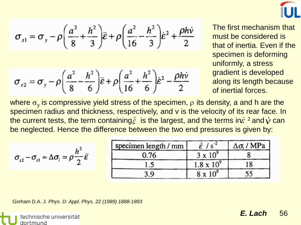
The first mechanism that must be considered is that of inertia. Even if the specimen is deforming uniformly, a stress gradient is developed along its length because of inertial forces.

Gorham D.A. J. Phys. D: Appl. Phys. 22 (1989) 1888-1893

where σy is compressive yield stress of the specimen, ρ its density, a and h are the specimen radius and thickness, respectively, and v is the velocity of its rear face. In the current tests, the term containing is the largest, and the terms in 2 and can be neglected. Hence the difference between the two end pressures is given by:

ε ε v

E. Lach 57

( ) ( ) ( )220

2

20

1(23

14raz −

+

−−= ε

εε

ερσ

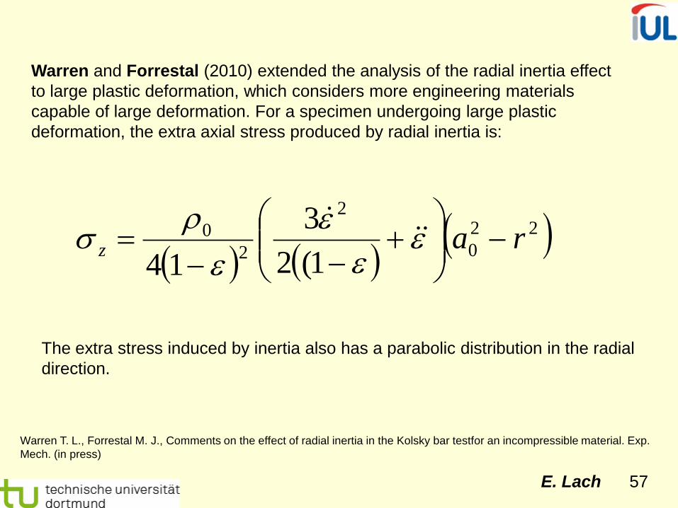
Warren and Forrestal (2010) extended the analysis of the radial inertia effect to large plastic deformation, which considers more engineering materials capable of large deformation. For a specimen undergoing large plastic deformation, the extra axial stress produced by radial inertia is:

The extra stress induced by inertia also has a parabolic distribution in the radial direction.

Warren T. L., Forrestal M. J., Comments on the effect of radial inertia in the Kolsky bar testfor an incompressible material. Exp. Mech. (in press)

E. Lach 58

E. Lach 59

E. Lach 60

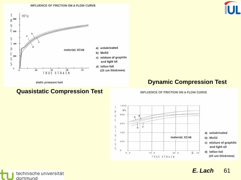
The influence of the friction is of great importance for the measured values of all compression tests including the dynamically executed tests. Lubrication has a high priority. The first scientists were more involved with the effects of longitudinal inertia, i. e. how long it lasts until the stress equilibrium is reached between both ends of the compression specimen.

Friction

E. Lach 61

Quasistatic Compression Test Dynamic Compression Test

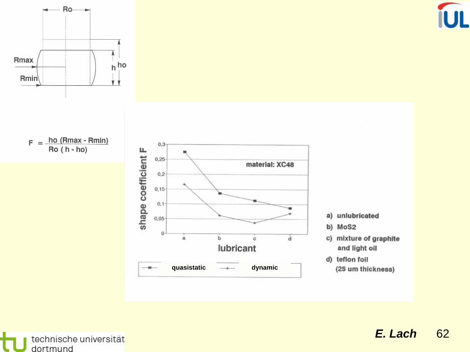
E. Lach 62

quasistatic dynamic

E. Lach 63

0

500

1000

1500

2000

2500

3000

0.0 0.1 0.2 0.3 0.4 0.5 0.6 0.7 0.8

TRU

E ST

RES

S

TRUE STRAIN

MPa

quasistatic5 x 10-3 s-1

dynamic5 x 103 s-1

Ni: grain size = 20 nm

specimen: D2mm x 2mm

specimen:D10mm x 2mm

dynamic

quasistatic

12

E. Lach 64

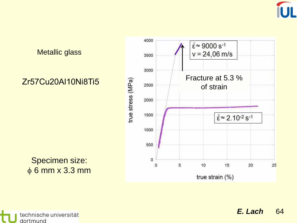
Metallic glass

Specimen size: φ 6 mm x 3.3 mm

Fracture at 5.3 % of strain

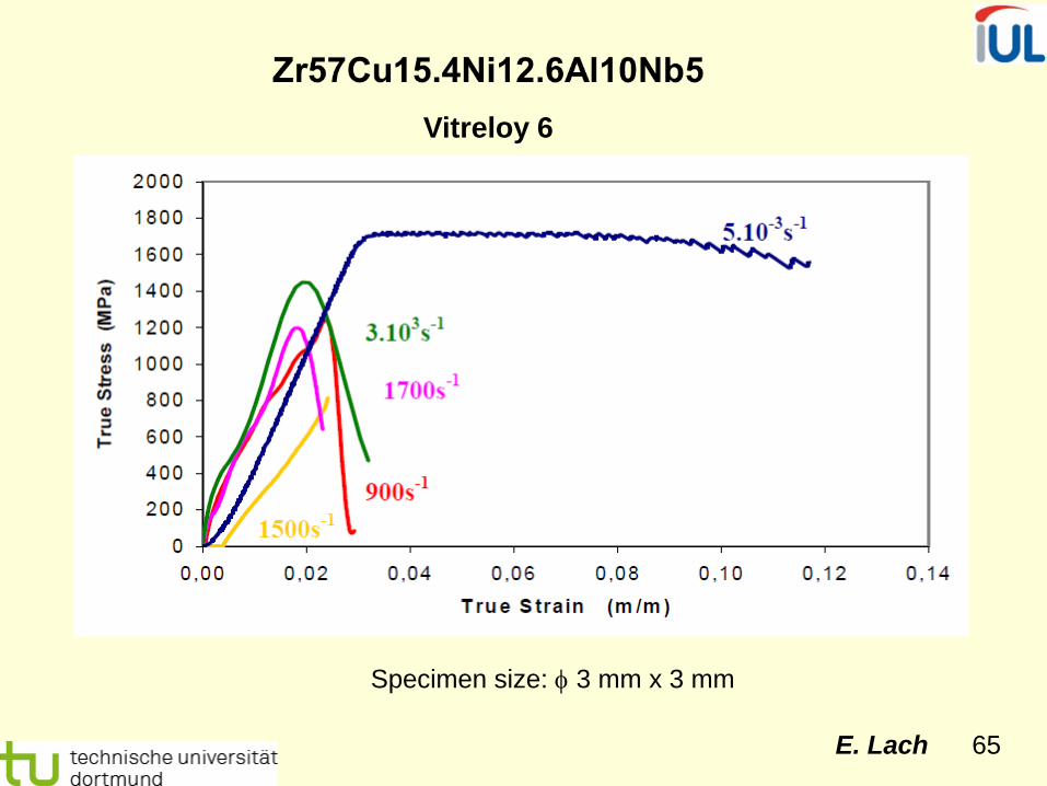
E. Lach 65

Vitreloy 6

Specimen size: φ 3 mm x 3 mm

E. Lach 66

Theory

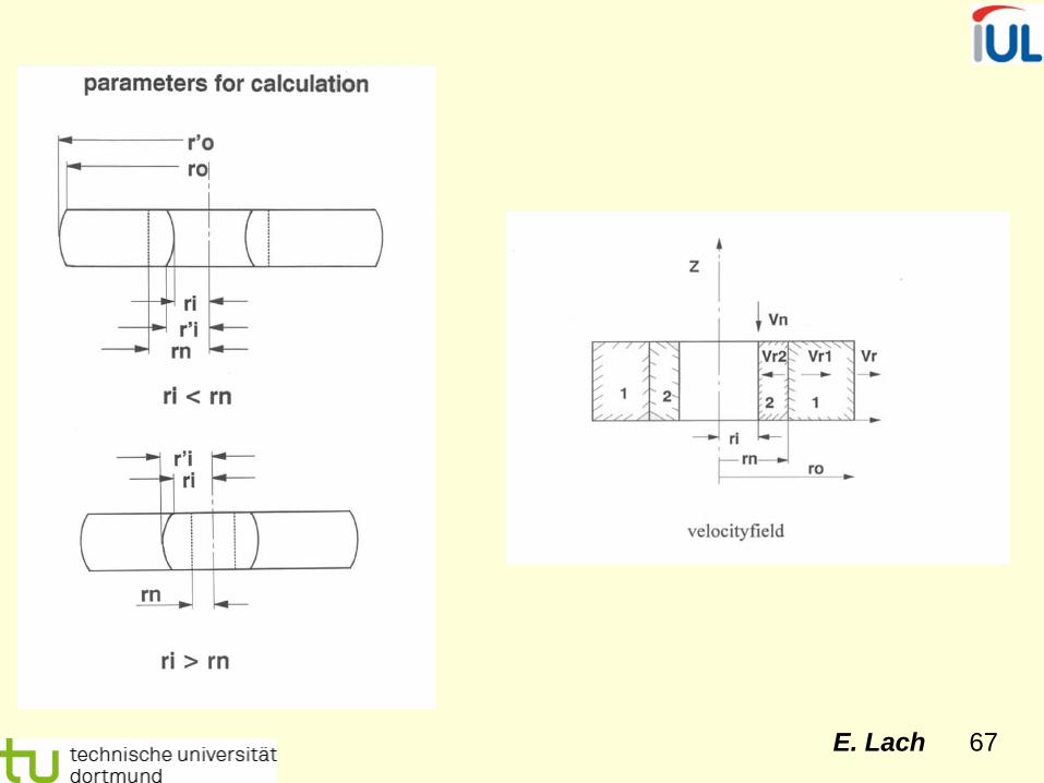
E. Lach 67

E. Lach 68

E. Lach 69

E. Lach 70

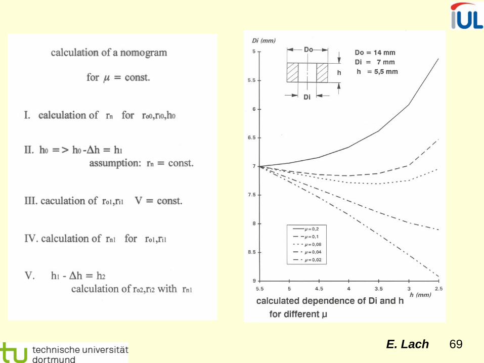
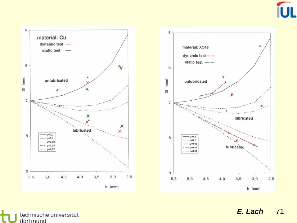
Ring Test Specimen

E. Lach 71

E. Lach 72

E. Lach 73

Using thinner specimens will help to achieve a more uniform deformation

state more quickly, but will increase the effects of friction

Gorham D.A., Pope P.H. and Cox 0.in Mechanical properties at high rates of strain 1984 ed. J. Harding (The Institute of Physics, Bristol, 1984) 151- 158

E. Lach 74

Summary of punching data for SHPB

Safa, K.; Gary, G.(2010); Displacement correction for punching at a dynamically loaded bar end, IE-1835, International Journal of Impact Engineering 37, 2010, 371-384

E. Lach 75

Extension of the incident wave length

When an incident bar is impacted by a low-impedance striker (Al and polymer), loading takes longer than when impacted by a striker of the same material (Al and Al).

12 vcccc

bbStSt

bbStSt

ρρρρσ

+⋅

−= 12 vcc

cvbbStSt

StSt

ρρρ

+=

T < T‘

E. Lach 76

The long split Hopkinson pressure bar (LSHPB)

B. Song & C.J. Syn & C.L. Grupido &W. Chen &W.-Y. Lu, A Long Split Hopkinson Pressure Bar (LSHPB) for Intermediate-rate Characterization of Soft Materials, Experimental Mechanics (2008) 48, p.809–815

A schematic presentation of the

LSHPB. The LSHPB setup

Fig. 1b: Details of connections A photograph

of a long SHPB

E. Lach 77

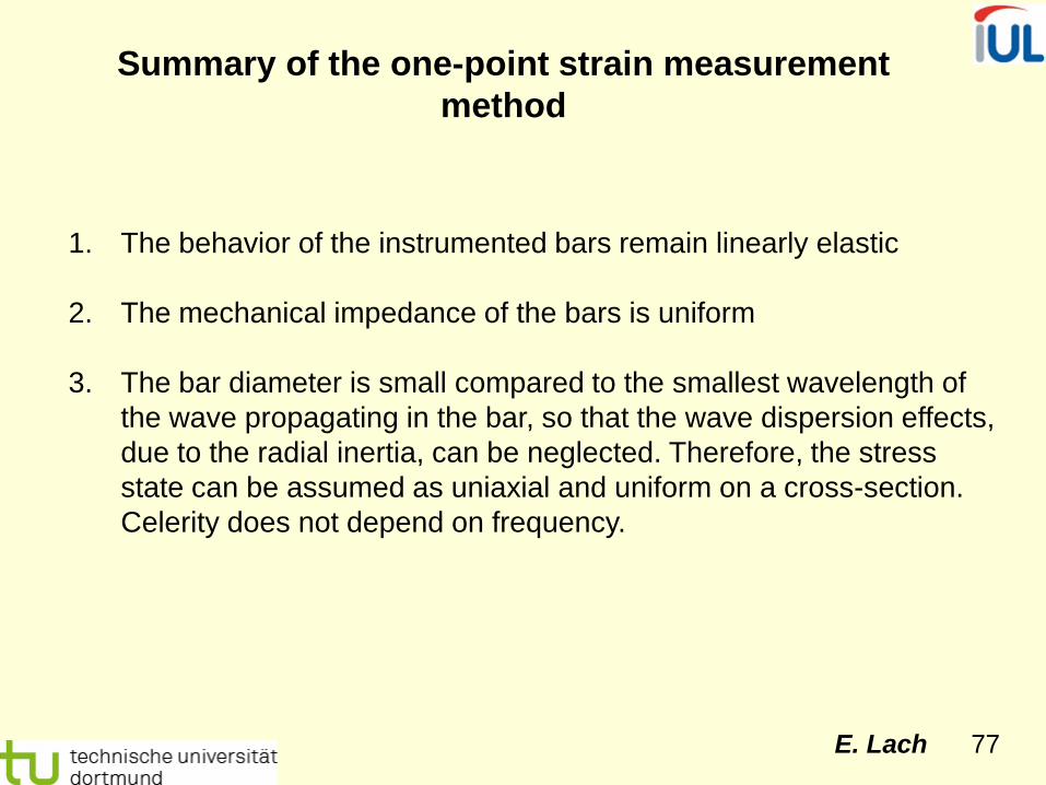
Summary of the one-point strain measurement method

1. The behavior of the instrumented bars remain linearly elastic

2. The mechanical impedance of the bars is uniform

3. The bar diameter is small compared to the smallest wavelength of the wave propagating in the bar, so that the wave dispersion effects, due to the radial inertia, can be neglected. Therefore, the stress state can be assumed as uniaxial and uniform on a cross-section. Celerity does not depend on frequency.

E. Lach 78

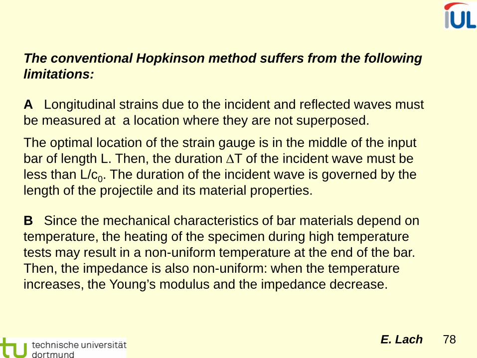
The conventional Hopkinson method suffers from the following limitations: A Longitudinal strains due to the incident and reflected waves must be measured at a location where they are not superposed.

The optimal location of the strain gauge is in the middle of the input bar of length L. Then, the duration ∆T of the incident wave must be less than L/c0. The duration of the incident wave is governed by the length of the projectile and its material properties. B Since the mechanical characteristics of bar materials depend on temperature, the heating of the specimen during high temperature tests may result in a non-uniform temperature at the end of the bar. Then, the impedance is also non-uniform: when the temperature increases, the Young’s modulus and the impedance decrease.

fundamentals of the split hopkinson pressure bar - iul · an impact produces compressive waves...

Documents