R

F

Aa

b

a

ARRAA

KdDDHM

C

h2n

Biomolecular Detection and Quantification 10 (2016) 15–23

Contents lists available at ScienceDirect

Biomolecular Detection and Quantification

j o ur na l ho mepage: www.elsev ier .com/ locate /bdq

eview Article

undamentals of multiplexing with digital PCR

lexandra S. Whalea,∗, Jim F. Huggetta, Svilen Tzonevb

Molecular and Cell Biology Team, LGC, Queens Road, Teddington, Middlesex TW11 0LY, United KingdomDigital Biology Centre, Bio-Rad Laboratories Inc., 5731 West Las Positas Boulevard, Pleasanton, CA 94588, United States

r t i c l e i n f o

rticle history:eceived 28 March 2016eceived in revised form 13 May 2016ccepted 17 May 2016vailable online 27 May 2016

a b s t r a c t

Over the past decade numerous publications have demonstrated how digital PCR (dPCR) enables preciseand sensitive quantification of nucleic acids in a wide range of applications in both healthcare and envi-ronmental analysis. This has occurred in parallel with the advances in partitioning fluidics that enable areaction to be subdivided into an increasing number of partitions. As the majority of dPCR systems arebased on detection in two discrete optical channels, most research to date has focused on quantification

eywords:PCRigital PCRuplexigher order multiplexingultiplexing

of one or two targets within a single reaction. Here we describe ‘higher order multiplexing’ that is theunique ability of dPCR to precisely measure more than two targets in the same reaction. Using examples,we describe the different types of duplex and multiplex reactions that can be achieved. We also describeessential experimental considerations to ensure accurate quantification of multiple targets.

© 2016 The Author(s). Published by Elsevier GmbH. This is an open access article under the CCBY-NC-ND license (http://creativecommons.org/licenses/by-nc-nd/4.0/).

ontents

1. Introduction . . . . . . . . . . . . . . . . . . . . . . . . . . . . . . . . . . . . . . . . . . . . . . . . . . . . . . . . . . . . . . . . . . . . . . . . . . . . . . . . . . . . . . . . . . . . . . . . . . . . . . . . . . . . . . . . . . . . . . . . . . . . . . . . . . . . . . . . . . . . . 161.1. Detection of amplification . . . . . . . . . . . . . . . . . . . . . . . . . . . . . . . . . . . . . . . . . . . . . . . . . . . . . . . . . . . . . . . . . . . . . . . . . . . . . . . . . . . . . . . . . . . . . . . . . . . . . . . . . . . . . . . . . . . . . . 161.2. Basics of quantification . . . . . . . . . . . . . . . . . . . . . . . . . . . . . . . . . . . . . . . . . . . . . . . . . . . . . . . . . . . . . . . . . . . . . . . . . . . . . . . . . . . . . . . . . . . . . . . . . . . . . . . . . . . . . . . . . . . . . . . . . .16

2. Duplex assays . . . . . . . . . . . . . . . . . . . . . . . . . . . . . . . . . . . . . . . . . . . . . . . . . . . . . . . . . . . . . . . . . . . . . . . . . . . . . . . . . . . . . . . . . . . . . . . . . . . . . . . . . . . . . . . . . . . . . . . . . . . . . . . . . . . . . . . . . . . 162.1. Non-competing duplex reactions (two primer pairs) . . . . . . . . . . . . . . . . . . . . . . . . . . . . . . . . . . . . . . . . . . . . . . . . . . . . . . . . . . . . . . . . . . . . . . . . . . . . . . . . . . . . . . . . . . 172.2. Competing duplex reactions (one primer pair with two probes binding the same region) . . . . . . . . . . . . . . . . . . . . . . . . . . . . . . . . . . . . . . . . . . . . . . . . . . . 172.3. Non-competing (hybrid) duplex reactions . . . . . . . . . . . . . . . . . . . . . . . . . . . . . . . . . . . . . . . . . . . . . . . . . . . . . . . . . . . . . . . . . . . . . . . . . . . . . . . . . . . . . . . . . . . . . . . . . . . . . 182.4. Duplexing using non-specific double stranded DNA binding dyes . . . . . . . . . . . . . . . . . . . . . . . . . . . . . . . . . . . . . . . . . . . . . . . . . . . . . . . . . . . . . . . . . . . . . . . . . . . . . 18

3. Higher order multiplexing . . . . . . . . . . . . . . . . . . . . . . . . . . . . . . . . . . . . . . . . . . . . . . . . . . . . . . . . . . . . . . . . . . . . . . . . . . . . . . . . . . . . . . . . . . . . . . . . . . . . . . . . . . . . . . . . . . . . . . . . . . . . . . 183.1. Amplitude-based multiplexing . . . . . . . . . . . . . . . . . . . . . . . . . . . . . . . . . . . . . . . . . . . . . . . . . . . . . . . . . . . . . . . . . . . . . . . . . . . . . . . . . . . . . . . . . . . . . . . . . . . . . . . . . . . . . . . . . 183.2. Ratio-based multiplexing with complete cluster identification . . . . . . . . . . . . . . . . . . . . . . . . . . . . . . . . . . . . . . . . . . . . . . . . . . . . . . . . . . . . . . . . . . . . . . . . . . . . . . . . 183.3. Ratio-based multiplexing with incomplete cluster identification. . . . . . . . . . . . . . . . . . . . . . . . . . . . . . . . . . . . . . . . . . . . . . . . . . . . . . . . . . . . . . . . . . . . . . . . . . . . . .193.4. Non-discriminating multiplexing . . . . . . . . . . . . . . . . . . . . . . . . . . . . . . . . . . . . . . . . . . . . . . . . . . . . . . . . . . . . . . . . . . . . . . . . . . . . . . . . . . . . . . . . . . . . . . . . . . . . . . . . . . . . . . . 20

4. Considerations for accurate quantification . . . . . . . . . . . . . . . . . . . . . . . . . . . . . . . . . . . . . . . . . . . . . . . . . . . . . . . . . . . . . . . . . . . . . . . . . . . . . . . . . . . . . . . . . . . . . . . . . . . . . . . . . . . . . 204.1. Linked targets . . . . . . . . . . . . . . . . . . . . . . . . . . . . . . . . . . . . . . . . . . . . . . . . . . . . . . . . . . . . . . . . . . . . . . . . . . . . . . . . . . . . . . . . . . . . . . . . . . . . . . . . . . . . . . . . . . . . . . . . . . . . . . . . . . . 204.2. Specificity. . . . . . . . . . . . . . . . . . . . . . . . . . . . . . . . . . . . . . . . . . . . . . . . . . . . . . . . . . . . . . . . . . . . . . . . . . . . . . . . . . . . . . . . . . . . . . . . . . . . . . . . . . . . . . . . . . . . . . . . . . . . . . . . . . . . . . . .204.3. Effects of partition specific competition (PSC) . . . . . . . . . . . . . . . . . . . . . . . . . . . . . . . . . . . . . . . . . . . . . . . . . . . . . . . . . . . . . . . . . . . . . . . . . . . . . . . . . . . . . . . . . . . . . . . . . . 204.4. Other factors that can effect quantification . . . . . . . . . . . . . . . . . . . . . . . . . . . . . . . . . . . . . . . . . . . . . . . . . . . . . . . . . . . . . . . . . . . . . . . . . . . . . . . . . . . . . . . . . . . . . . . . . . . . . 214.5. Suggested experimental setup to assess dPCR assays . . . . . . . . . . . . . . . . . . . . . . . . . . . . . . . . . . . . . . . . . . . . . . . . . . . . . . . . . . . . . . . . . . . . . . . . . . . . . . . . . . . . . . . . . . 21

5. Conclusions . . . . . . . . . . . . . . . . . . . . . . . . . . . . . . . . . . . . . . . . . . . . . . . . . . . . . . . . . . . . . . . . . . . . . . . . . . . . . . . . . . . . . . . . . . . . . . . . . . . . . . . . . . . . . . . . . . . . . . . . . . . . . . . . . . . . . . . . . . . . . 21

Competing interest . . . . . . . . . . . . . . . . . . . . . . . . . . . . . . . . . . . . . . . . . . . . . . . . . . . . . . . . .Acknowledgments . . . . . . . . . . . . . . . . . . . . . . . . . . . . . . . . . . . . . . . . . . . . . . . . . . . . . . . . .

References . . . . . . . . . . . . . . . . . . . . . . . . . . . . . . . . . . . . . . . . . . . . . . . . . . . . . . . . . . . . . . . . . .

∗ Corresponding author.E-mail address: alexandra.whale@lgcgroup.com (A.S. Whale).

ttp://dx.doi.org/10.1016/j.bdq.2016.05.002214-7535/© 2016 The Author(s). Published by Elsevier GmbH. This is an open access ard/4.0/).

. . . . . . . . . . . . . . . . . . . . . . . . . . . . . . . . . . . . . . . . . . . . . . . . . . . . . . . . . . . . . . . . . . . . . . . . . . . . 22. . . . . . . . . . . . . . . . . . . . . . . . . . . . . . . . . . . . . . . . . . . . . . . . . . . . . . . . . . . . . . . . . . . . . . . . . . . . . 22

. . . . . . . . . . . . . . . . . . . . . . . . . . . . . . . . . . . . . . . . . . . . . . . . . . . . . . . . . . . . . . . . . . . . . . . . . . . . 22

ticle under the CC BY-NC-ND license (http://creativecommons.org/licenses/by-nc-

1 ction a

1

tttnqetmnbvtd

mohcimabitd[eni

1

cacscsisaathsftd

1

todts‘r

�

6 A.S. Whale et al. / Biomolecular Dete

. Introduction

Digital PCR (dPCR) involves the partitioning of a PCR reac-ion into a number of smaller partitions so that a proportion ofhem contain no template molecules [1,2]. PCR is then performedo determine the proportion of positive (with amplification) andegative (no amplification) partitions. This subdivision enablesuantification to be performed using established statistical mod-ls that are independent of a calibration curve [3] and increaseshe precision of the quantification [4–8]. There are two broad

echanisms for the subdivision of a reaction: partitioning usinganofluidics to load the reaction into prefabricated chambers, ory generation of water-in-oil emulsions. The partition volume canary from 4.4 �L down to 5 pL and the partition number in a reac-ion can vary from 496 up to 10 million partitions depending on thePCR platform used [9].

dPCR has been used in a wide range of research areas that includeeasurement of copy number variation in genetically modified

rganisms [10,11] and for karyotyping plants [12,13] as well as inuman disease models such as gene expression [14] and epigeneticontrol of gene expression in cancer [8,15,16], gene amplificationn cancer [6,17] and prenatal fetal karyotyping [18]. The other

ajor application for dPCR is in the detection of rare sequence vari-nts, which in standard qPCR can be lost within the high abundantackground type [17,19]. Such measurements have been evaluated

n many human diagnostic areas that include cancer stratifica-ion [20,21], antimicrobial resistance monitoring [22,23], prenataliagnostics [24,25] and monitoring of transplant organ rejection26]. Most recently, dPCR is finding multiple applications in themerging field of liquid biopsy, where solid tumors are profiledon-invasively based on detection of tumor-related nucleic acids

n blood or other anatomical liquids [27–29].

.1. Detection of amplification

dPCR relies on the ability to distinguish between partitions thatontain amplicons and those that do not. Partitions that containmplicons can be identified by the presence of increased fluores-ence using a variety of detection chemistries common to qPCRuch as intercalating DNA dyes or fluorophore-labelled oligonu-leotides [30]. Following PCR cycling, the fluorescence end-pointignal associated with each partition is measured by the readernstrument. This signal can be plotted on a one-dimensional (1D)catter graph, with the event (partition) number along the x-axisnd the fluorescent amplitude along the y-axis. In a well optimizedssay, two visually distinct populations are observed; positive par-itions that have high fluorescence, and negative partitions thatave low (or background) fluorescence. An automatic threshold iset by the software to separate these two populations, however,or all the dPCR platforms it is possible for the user to manually sethe threshold in the analysis software and this is described in moreetail in Section 4.4.

.2. Basics of quantification

Experimentally, we can only distinguish between negative par-itions (containing zero targets) and positive partitions (containingne or more targets). The fundamental assumption of independentistribution of target molecules into equal volume partitions meanshat the number of targets per partition will follow a standard Pois-on distribution. The Poisson model is defined by a single parameter�’—the average number of targets per partition. Historically, � is

epresented as:

= − ln(

1 − k

n

)(1)

nd Quantification 10 (2016) 15–23

where n is the total number of partitions detected and k is thenumber of positive partitions detected as defined in the “MinimumInformation for Publication of Quantitative Digital PCR Experi-ments” (dMIQE) guidelines (3). Eq. (1) is written in this way touse the positive partitions (k) as a proportion of total partitions(n). These were chosen as working with positive partitions is moreintuitive to the user. However, � is really calculated using the neg-ative partitions as the proportion of positive partitions in Eq. (1),k/n is subtracted from 1.

The negative partitions are arguably more informative than thepositive partitions since we know each negative partition containszero copies of the target, while a positive partition may contain oneor more copies of the target. When multiplexing, � needs to be cal-culated for each targets individually and the notion of a positivepartition becomes dependent on the target of interest. In a sensea ‘positive’ partition becomes even less informative as it may con-tain 1 or more copies of multiple targets. If w denotes the numberof partitions that are negative for a target and so n = k + w. By sub-stituting w into Eq. (1) we can calculate � in terms of the numberof negative partitions, � = −ln (w/n), that can then be rearranged togive Eq. (2):

� = ln (n) − ln (w) (2)

This arrangement allows for easier generalization in the case ofmultiple targets. The full advantage of Eq. (2) is realised when wewant to quantify a target in a sample without using all the parti-tions in that reaction. Specific scenarios and examples where thisis useful are given below in the relevant sections along with theappropriate generalization of Eq. (2).

For any given experiment, both Eqs. (1) and (2) provide an esti-mate of � and the uncertainty of � can be calculated using equationsthat are described elsewhere [6,31]. In certain cases the assumptionof independent target distribution may not hold, for example, withclose tandem copies [6] or denatured DNA [32,33]. Furthermore,molecular dropout may occur, where a molecule fails to amplifyand so a partition that initially contained a molecule is wronglyclassified as negative [34]. In such cases the estimate of � will notbe accurate as the binomial distribution is no longer appropriate.

2. Duplex assays

Duplex assays enable concurrent amplification of two targetswithin a single reaction. This reduces technical errors, such asaccumulated pipetting inaccuracy, thereby making it possible tomeasure smaller differences than the same comparison using par-allel uniplex reactions [34]. Duplexing also reduces reagent andtime needs. Duplex assays can be performed with intercalating DNAdyes or fluorophore-labelled oligonucleotides; the examples illus-trated in this study use hydrolysis probes, but the theory holdstrue for other fluorophore-labelling strategies such as Scorpionor AmplifluorTM primer-probes or hybridisation probes such asMolecular Beacons [30].

In duplex hydrolysis probe assays, the two probes are typicallylabelled with a different dye to match the two detection channels.There are four possible configurations in terms of the number ofprimer pairs used in the reaction (1 or 2) and if the two probes bindthe same region of the generated amplicon(s) (Table 1). Only threeconfigurations are meaningful, since the fourth one is unlikely tooccur where different primers generate amplicons containing thesame probe binding site.

An alternative strategy for duplex reactions is to use a single-colour intercalating DNA dye, such as EvaGreen, to amplifyamplicons of different sizes for the different targets; the targetsare discriminated by the differences in the fluorescence ampli-

A.S. Whale et al. / Biomolecular Detection and Quantification 10 (2016) 15–23 17

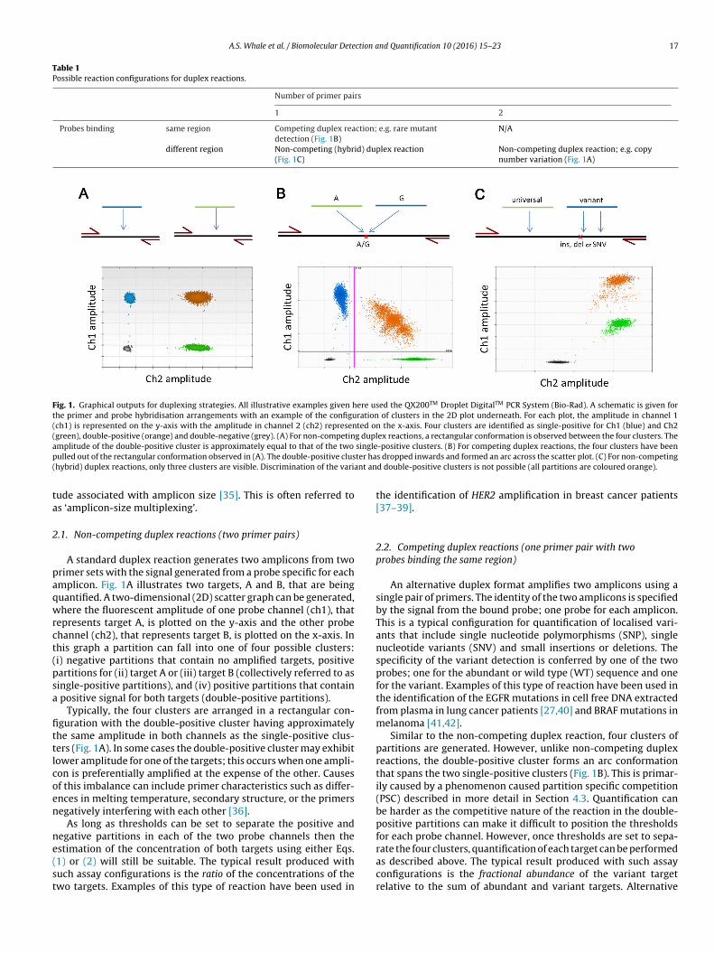
Table 1Possible reaction configurations for duplex reactions.

Number of primer pairs

1 2

Probes binding same region Competing duplex reaction; e.g. rare mutantdetection (Fig. 1B)

N/A

different region Non-competing (hybrid) duplex reaction(Fig. 1C)

Non-competing duplex reaction; e.g. copynumber variation (Fig. 1A)

Fig. 1. Graphical outputs for duplexing strategies. All illustrative examples given here used the QX200TM Droplet DigitalTM PCR System (Bio-Rad). A schematic is given forthe primer and probe hybridisation arrangements with an example of the configuration of clusters in the 2D plot underneath. For each plot, the amplitude in channel 1(ch1) is represented on the y-axis with the amplitude in channel 2 (ch2) represented on the x-axis. Four clusters are identified as single-positive for Ch1 (blue) and Ch2(green), double-positive (orange) and double-negative (grey). (A) For non-competing duplex reactions, a rectangular conformation is observed between the four clusters. Thea singlep ter ha( nt an

ta

2

paqwrct(psa

fittlcoen

ne(st

mplitude of the double-positive cluster is approximately equal to that of the two

ulled out of the rectangular conformation observed in (A). The double-positive clushybrid) duplex reactions, only three clusters are visible. Discrimination of the varia

ude associated with amplicon size [35]. This is often referred tos ‘amplicon-size multiplexing’.

.1. Non-competing duplex reactions (two primer pairs)

A standard duplex reaction generates two amplicons from tworimer sets with the signal generated from a probe specific for eachmplicon. Fig. 1A illustrates two targets, A and B, that are beinguantified. A two-dimensional (2D) scatter graph can be generated,here the fluorescent amplitude of one probe channel (ch1), that

epresents target A, is plotted on the y-axis and the other probehannel (ch2), that represents target B, is plotted on the x-axis. Inhis graph a partition can fall into one of four possible clusters:i) negative partitions that contain no amplified targets, positiveartitions for (ii) target A or (iii) target B (collectively referred to asingle-positive partitions), and (iv) positive partitions that contain

positive signal for both targets (double-positive partitions).Typically, the four clusters are arranged in a rectangular con-

guration with the double-positive cluster having approximatelyhe same amplitude in both channels as the single-positive clus-ers (Fig. 1A). In some cases the double-positive cluster may exhibitower amplitude for one of the targets; this occurs when one ampli-on is preferentially amplified at the expense of the other. Causesf this imbalance can include primer characteristics such as differ-nces in melting temperature, secondary structure, or the primersegatively interfering with each other [36].

As long as thresholds can be set to separate the positive andegative partitions in each of the two probe channels then the

stimation of the concentration of both targets using either Eqs.1) or (2) will still be suitable. The typical result produced withuch assay configurations is the ratio of the concentrations of thewo targets. Examples of this type of reaction have been used in

-positive clusters. (B) For competing duplex reactions, the four clusters have beens dropped inwards and formed an arc across the scatter plot. (C) For non-competingd double-positive clusters is not possible (all partitions are coloured orange).

the identification of HER2 amplification in breast cancer patients[37–39].

2.2. Competing duplex reactions (one primer pair with twoprobes binding the same region)

An alternative duplex format amplifies two amplicons using asingle pair of primers. The identity of the two amplicons is specifiedby the signal from the bound probe; one probe for each amplicon.This is a typical configuration for quantification of localised vari-ants that include single nucleotide polymorphisms (SNP), singlenucleotide variants (SNV) and small insertions or deletions. Thespecificity of the variant detection is conferred by one of the twoprobes; one for the abundant or wild type (WT) sequence and onefor the variant. Examples of this type of reaction have been used inthe identification of the EGFR mutations in cell free DNA extractedfrom plasma in lung cancer patients [27,40] and BRAF mutations inmelanoma [41,42].

Similar to the non-competing duplex reaction, four clusters ofpartitions are generated. However, unlike non-competing duplexreactions, the double-positive cluster forms an arc conformationthat spans the two single-positive clusters (Fig. 1B). This is primar-ily caused by a phenomenon caused partition specific competition(PSC) described in more detail in Section 4.3. Quantification canbe harder as the competitive nature of the reaction in the double-positive partitions can make it difficult to position the thresholdsfor each probe channel. However, once thresholds are set to sepa-

rate the four clusters, quantification of each target can be performedas described above. The typical result produced with such assayconfigurations is the fractional abundance of the variant targetrelative to the sum of abundant and variant targets. Alternative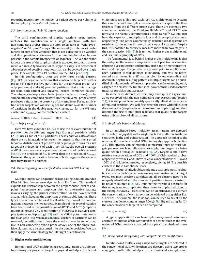

1 ction a

rt

2

inntaptmap

(ponTsptoc

�

�

pEtbto[Ht

2d

Depiatthmptrlit

3

t

8 A.S. Whale et al. / Biomolecular Dete

eporting metrics are the number of variant copies per volume ofhe sample, e.g. copies/mL of plasma.

.3. Non-competing (hybrid) duplex reactions

The third configuration of duplex reactions using probesncludes the amplification of a single amplicon with twoon-competing probes; these are often referred to as “Wild-Type-egative” or “drop-off” assays. The universal (or reference) probeargets an area of the amplicon that is not expected to be variablend thus, provides a reference for the total number of moleculesresent in the sample irrespective of sequence. The variant probeargets the area of the amplicon that is expected to contain one or

ore variants. A typical use for this type of assay is in detection of broader set of possible mutations than can be covered by a singlerobe, for example, exon 19 deletions in the EGFR gene [27].

In this configuration, there are only three visible clustersFig. 1C): (i) negative partitions that contain no targets for eitherrobe, (ii) single-positive partitions for the universal probe (WTnly partitions) and (iii) positive partitions that contain a sig-al from both variant and universal probes (combined cluster).he missing single-positive cluster (variant only partitions) is sub-umed into the combined cluster since the universal probe alwaysroduces a signal in the presence of any amplicon. For quantifica-ion of the targets we will use Eq. (2) and define c0 as the numberf partitions in the double-negative cluster, cwt for the WT onlyluster and ccombined for the combined cluster:

variant = ln (c0 + cwt + ccombined) − ln (c0 + cwt) (3)

wt = ln (c0 + cwt) − ln (c0) (4)

Here we have extended Eq. (2) to use the relevant number ofartitions for the different targets. Eq. (3) uses all partitions, whileq. (4) uses a subset of all partitions. These equations also assumehere are no interactions between the targets so that the a prioriinomial distributions of positive and negative partitions for eacharget are independent of each other. Since, the overall precisionf dPCR measurements depends on the number of partitions used43,44], the precision of �wt is lower than the precision of �variant .owever, the quantification trueness of both targets is the same in

hat they are both unbiased.

.4. Duplexing using non-specific double stranded DNA bindingyes

Multiple targets can be quantified using a single double strandedNA binding fluorescence dye, such as EvaGreen. This methodxploits the relationship between the proportionate level of end-oint fluorescence and amplicon size. An alternative strategy

nvolves varying the primer concentration for the two differentssays, whilst keeping the amplicons at comparable lengths. Theseypes of reaction can be used to calculate the ratio of the concen-rations between the two targets. Examples of this type of reactionave been used in the quantification of RPP30 and ACTB (ampliconultiplexing) and CNV identification of MRGPRX1 in HapMap sam-

les (primer multiplexing) [35] and the V600E point mutation inhe BRAF gene [45]. When all canonical clusters of partitions can beesolved, quantification is done the standard way. In some cases,ike in non-competing hybrid probe assays, one of the single pos-tive clusters may be subsumed into the double positives. We canhen apply the same strategy for full target quantification.

. Higher order multiplexing

In traditional qPCR multiplexing reactions, targets are differen-iated using one probe per target conjugated with dyes of different

nd Quantification 10 (2016) 15–23

emission spectra. This approach restricts multiplexing to systemsthat can cope with multiple emission spectra to capture the fluo-rescence from the different probe dyes. There are currently twocommercial systems, the Fluidigm BioMarkTM and EP1TM sys-tems and the recently commercialised Stilla NarciaTM System, thathave the capacity to multiplex in four and three optical channels,respectively. The other commercially available dPCR systems arerestricted to detection in two discrete optical channels. Despitethis, it is possible to precisely measure more than two targets inthe same reaction [46]. This is termed ‘higher order multiplexing’and is a unique property of dPCR.

The fundamental idea behind higher order multiplexing is thatthe end-point fluorescence amplitude in each partition is a functionof probe-dye conjugation and mixing, probe and primer concentra-tions and the type of targets that are present prior to amplification.Each partition is still detected individually and will be repre-sented as an event in a 2D scatter plot. By understanding anddeconvoluting the resulting patterns, multiple targets can be quan-tified simultaneously. When each partition can be unambiguouslyassigned to a cluster, the full statistical power can be used to achievemaximal precision and accuracy.

In some cases different clusters may overlap in 2D space and,as we observed with the non-competing duplex reactions (Section2.3), it is still possible to quantify specifically, albeit at the expenseof reduced precision. We will first cover the cases with full clusterdiscrimination (amplitude- or ratio-based multiplexing) and thendescribe the use of multiplex reactions that quantify the targetsusing only a subset of all partitions.

3.1. Amplitude-based multiplexing

In an amplitude-based multiplex assay, targets are detectedwith probes conjugated with a single dye but at a different final con-centration in the end-point reaction. This approach is similar to thenon-specific double stranded DNA binding dye approach (Section2.4). This strategy can be modified to measure three or more tar-gets per reaction. In our illustrated example, four targets are beingquantified in a ‘tetraplex’ reaction (Fig. 2A). Targets A and B haverelative concentrations of 50% and 100% of Ch2-labelled probes,respectively; while C and D have relative concentrations of 50% and100% of Ch1-labelled probes, respectively, giving 16 (24) possibleclusters in the 2D amplitude space.

For this set up, single, double, triple and quadruple-positive clus-ters arise as a partition can contain any combination of the targettypes. For most precise quantification, all 16 clusters need to beuniquely identified and the number of partitions in each cluster tobe reliably counted (Fig. 2A). Defining the threshold positions forthis set up is more complicated than those for duplex reactions. Inthe example shown, all 16 clusters can be identified and so estimatethe concentration of each target can be achieved using either Eqs.(1) or (2). For example, the lasso tool can be used to select all theclusters that do not contain target B (wB) (Fig. 2B) and using Eq. (2),the concentration of target B can be computed:

� = ln (n) − ln (wB) (5)

A typical application for such multiplex assays could be for moreaccurate estimation of the copy number of a target such as the eval-uation of DNA integrity extracted from paraffin embedded tissue[47].

3.2. Ratio-based multiplexing with complete cluster identification

In ratio-based multiplexing assays some targets are detected inthe conventional way, while others are detected using two probesconjugated with different dyes. In the illustrated example three

A.S. Whale et al. / Biomolecular Detection and Quantification 10 (2016) 15–23 19

Fig. 2. Graphical outputs for higher order multiplexing strategies. All illustrative examples given here used the QX200TM Droplet DigitalTM PCR System (Bio-Rad). For eachmultiplexing strategy a schematic and worked example of the configuration of clusters in the 2D plot is given with the amplitude in channel 1 (ch1) is represented on they-axis with the amplitude in channel 2 (ch2) is represented on the x-axis. For each schematic the approximate location of the single target positive clusters are identified assolid coloured circles with the double or triple target positive clusters are shown as dotted circles. For the worked examples, the clusters are not pseudocoloured according tothe target due to the limitations of the software. (A) For amplitude-based multiplexing, four independent targets are being quantified: targets A (100% Ch2-labelled probe),B (100% Ch2), C (50% Ch1) and D (100% Ch1) giving 16 possible clusters in the 2D amplitude space. For the worked example, all the clusters containing partitions that do notcontain target B are lassoed (wB). (B) For ratio-based multiplexing, three independent targets are being quantified: targets A (100% Ch2), B (100% Ch1) and C (50% Ch2 and 50%Ch1) giving 8 possible clusters in the 2D amplitude space. For the worked example, the four clusters used in the quantification are lassoed and labelled: negative cluster for alltargets (c0), single-positive for target B (cB), single-positive for target A (cA), and double-positive for targets A and B (cAB). (C) For ratio-based non-discriminating multiplexing,five targets are being quantified: targets A (100% Ch2), B (75% Ch2/25%Ch1), C (50% Ch2/50% Ch1), D (25% Ch2/75% Ch1) and E (100% Ch1). A total of 32 combinations ofclusters are possible, however, due to the ratios of the probes for the different targets, most are not uniquely identifiable. For example, a cluster containing both targets A andD (125% Ch2/75% Ch1) would not be distinguishable from a cluster containing both targets B and C (also 125% Ch2/75% Ch1). Therefore only the single-positive clusters can beused in the quantification. For the worked example, the two clusters used for the quantification of target D are lassoed: negative cluster for all targets (c0) and single-positivecluster for target D (c ). (D) For non-discriminating multiplexing the example of the KRAS mutations in codons 12 and 13 is shown. The 7 probes for the mutant SNVs area the Cw t is noq

ttr5sbI(t

nHiFtdtn

n

w

o

�

atsa

D

�D = ln (c0 + cD) − ln (c0) (9)

D

ll conjugated with the Ch1-labelled probe and the WT probe is conjugated withith a single cluster in the WT channel. The double-positive cluster is also visible. I

uantification of the total number of mutant sequences only.

argets are being quantified (Fig. 2B). Targets A and B have rela-ive concentrations of 100% Ch2- and 100% Ch1-labelled probes,espectively. Target C has relative concentrations of 50% Ch2- and0% Ch1-labelled probes. The expected location of the target Cingle-positive cluster is in between those of targets A and B, whereoth probe channels have a 50% reduction in fluorescent amplitude.

ncluding the double- and triple-positive clusters gives a total of 823) identifiable clusters for all possible combinations of the threeargets.

In this example, we can use either Eqs. (1) or (2) to quantify theumber of target molecules as described in the previous section.owever, the full advantage of using Eq. (2) over Eq. (1) can be

llustrated when we want to quantify based on a subset of clusters.or example, we might want to exclude all clusters that containarget C from the quantification and so use only the clusters thato not contain target C (Fig. 2B). Therefore, the total number ofhe partitions in the reaction and the number of partitions that areegative for target B are defined as:

notC = c0 + cA + cB + cAB (6)

B = c0 + cA (7)

From this we can then use Eq. (2) to estimate the concentrationf target B:

B = ln (c0 + cA + cB + cAB) − ln (c0 + cA) (8)

Whether we use all partitions or a subset of partitions, we will

chieve unbiased estimates, as long as there is no linkage betweenhe targets (see Section 4.1). We may need to use fewer clusters ifome clusters are not uniquely identifiable, poorly defined or notll accounted for in the reaction (a sample may not contain target

h2-labelled probe. Three diffuse clusters are visible in the mutant probe channelt possible to discriminate between the 3 mutant clusters and so this set up allows

C). Again, this method enables us to preserve the accuracy whilegiving some ground on precision.

3.3. Ratio-based multiplexing with incomplete clusteridentification

In some cases, a careful selection of the ratios of the probeswould allow an operator to multiplex even more targets in a singlereaction. This may require use of an incomplete set of clusters. Inthe illustrated example five targets are quantified (Fig. 2C). TargetsA and E have relative concentrations of 100% Ch2 and Ch1-labelledprobes, respectively. Targets B, C and D have labelled Ch1 and Ch2-labelled probes at varying ratios. In this setup we should see a totalof 32 (25) different combinations of the five targets; however, manyof these clusters may not be uniquely identifiable. For example, theposition of the double-positive partitions containing targets A andD may overlap with that of the double-partitions containing targetsB and C (Fig. 2C). In many cases higher order positives also cannot beuniquely identified. Nevertheless, one can achieve accurate quan-tification by using only the single-positive clusters. For example, tocalculate the concentration of target D using Eq. (2) we only needto count the number of partitions in the negative cluster (c0) andthe single-positive cluster that contains target D (c ) (Fig. 2C):

This method allows for interrogation of multiple targets at theexpense of reduced precision. As before the estimates for averageoccupancies for each target are unbiased.

20 A.S. Whale et al. / Biomolecular Detection and Quantification 10 (2016) 15–23

Fig. 3. Considerations for accurate quantification. All illustrative examples given here used the QX200TM Droplet DigitalTM PCR System (Bio-Rad) using duplex reactions;however, all of these are relevant for higher order multiplexing strategies. (A) For the analysis of a probe-competing duplex reactions to quantify a transition mutation.C bes ors the foa t caus

3

tiics1pw

dtumpstu2

4

tctstbtihf

4

abtqtaWaC

ross-hybridisation of the probes caused by either mismatched binding of the proingle-positive clusters. This can impact on positioning the thresholds to separate

cid deletion mutation to illustrate that mismatched binding of the probes does no

.4. Non-discriminating multiplexing

To complete our survey of multiplexing assays we next describehe case where some targets are detected but will never be uniquelydentified as this is not required by the application. In such exper-ments, we wish to report the presence and quantity of anyombination of the targets of interest. A typical example is pre-ented in Fig. 2D where all 7 mutations in the KRAS gene, exons2 and 13, are Ch1-labelled probes, while WT has a Ch2-labelledrobe. The 7 mutant species generate 3 diffuse mutant clusters bute combine the counts of those for the purposes of quantification.

Identification of the specific mutation is not required as the fun-amental question is ‘does this sample contain mutations’ and sohe reaction performs a screening role. Such screening assays areseful when the expected prevalence of mutations is low and it isore efficient to only determine the specific mutation in the sam-

le once the presence of a mutation has been confirmed. Multiplexcreening in this style typically leads to reduced sensitivity limitshan when detecting individual targets. For quantification we canse Eq. (2) as described for competing duplex reactions (Section.2).

. Considerations for accurate quantification

Several factors are important for accurate quantification of mul-iplexed assays. These include target linkage, probe specificity andompetition, differential PCR efficiencies. Any factor that distortshe location and uniqueness of clusters needs to be taken into con-ideration, especially when multiple targets are measured. Due tohe extra level of complexity in these types of reactions, care shoulde taken to recognise and reduce these effects by rigorous optimisa-ion to ensure accurate estimation of �. In this section we describen more detail the causes of these factors and the effects they canave on the quantification if they are not recognised and accounted

or.

.1. Linked targets

Quantification of linked targets by dPCR may cause problemss the assumptions for random and independent (Poisson) distri-ution of target molecules may not hold. Tandem repeat copies ofhe same target would co-localize in the same partition more fre-uently than by chance, which will lead to an underestimation ofhe true number of copies. In the case of two different targets in cis

nd nearby, there will be an excess of double positive partitions.e can measure the concentration of each target using standard

pproaches but may miss the fact the targets are indeed linked [48].urrent standard analysis tools can report the concentration of the

filter bleed-though can be visualised as a ‘leaning’ (blue) or ‘lifting’ (green) of theur clusters. (B) Analysis of a probe-competing duplex reaction to detect a 3 aminoe the ‘leaning’ or ‘lifting’ of the clusters compared with that observed in (A).

linked molecules using linkage-based assays to measure cis versustrans configuration of targets and potential structural rearrange-ments [49]. This can be further extended to determine the degreeof DNA fragmentation under different extraction conditions. Careneeds to be taken when using a reduced set of clusters for quantifi-cation as this approach is in general valid under the assumption ofno linkage or higher order target correlations.

4.2. Specificity

The design of an assay for detection of SNVs is naturally some-what constrained. In an ideal scenario, the two probes will havestringent enough specificity, such that only ‘fully matched hybridi-sation’ will occur; the WT probe will hybridise to the ampliconscontaining the WT sequence only and the variant probe willhybridise to the amplicons containing the mutant sequence only.However, for many SNV assays, cross-(mismatched) hybridisationof the probes does occur. As mismatches occur with lower efficiencythan matches, this will lead to ‘leaning’ or ‘lifting’ of the single-positive partitions in the 2D scatter plot (Fig. 3A). For comparison,cross-hybridisation is less pronounced when the probe targets avariation involving two or more nucleotide deletions or insertions(Fig. 3B).

This loss of specificity can be further compounded by opticalbleed-through, where the fluorescence from a dye is picked up byboth detection channels (often referred to as ‘filter cross-talk’). Thiseffect produces a similar ‘lifting’ of the clusters and may be hardto separate from probe cross-hybridization effects. Filter cross talkcan be alleviated by careful selection of conjugated dyes that matchoptical detection systems and by adjustment of signal processingparameters in the analysis software where this is possible.

4.3. Effects of partition specific competition (PSC)

In dPCR any partition is a miniature reaction by itself. As such,competition effects during PCR may be present. The degree to whichthose matter will depend on factors such as which targets andhow many molecules of each target are present in each partition,differential amplification efficiencies, DNA accessibility and tem-plate quality. Every partition will follow standard amplificationtrajectory with an early exponential amplification followed by asaturation phase.

For CNV-like duplex assays (Section 2.1), there is no direct probecompetition. However, in the double-positive partitions (where

both targets are present at start) there will be two PCR reactionscompeting for resources. In the case where efficiencies are roughlybalanced, the amplitudes of the double-positive partitions will besimilar to the amplitudes of single-positive partitions. An imbal-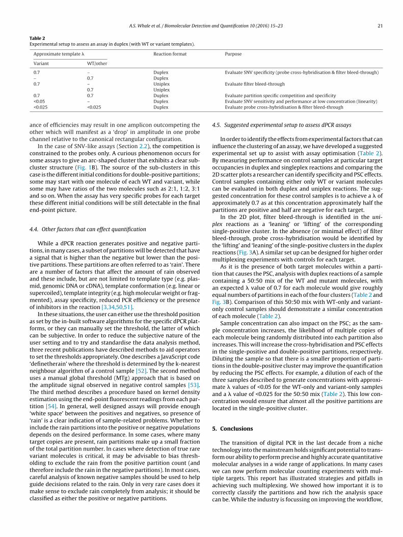

A.S. Whale et al. / Biomolecular Detection and Quantification 10 (2016) 15–23 21

Table 2Experimental setup to assess an assay in duplex (with WT or variant templates).

Approximate template � Reaction format Purpose

Variant WT/other

0.7 – Duplex Evaluate SNV specificity (probe cross-hybridisation & filter bleed-through)– 0.7 Duplex0.7 – Uniplex Evaluate filter bleed-through

0.7 Uniplex

aoc

csccssate

4

tataamsmo

afcutt‘nutTet‘‘idtovotcgmc

0.7 0.7 Duplex

<0.05 – Duplex

<0.025 <0.025 Duplex

nce of efficiencies may result in one amplicon outcompeting thether which will manifest as a ‘drop’ in amplitude in one probehannel relative to the canonical rectangular configuration.

In the case of SNV-like assays (Section 2.2), the competition isonstrained to the probes only. A curious phenomenon occurs forome assays to give an arc-shaped cluster that exhibits a clear sub-luster structure (Fig. 1B). The source of the sub-clusters in thisase is the different initial conditions for double-positive partitions;ome may start with one molecule of each WT and variant, whileome may have ratios of the two molecules such as 2:1, 1:2, 3:1nd so on. When the assay has very specific probes for each targethese different initial conditions will be still detectable in the finalnd-point picture.

.4. Other factors that can effect quantification

While a dPCR reaction generates positive and negative parti-ions, in many cases, a subset of partitions will be detected that have

signal that is higher than the negative but lower than the posi-ive partitions. These partitions are often referred to as ‘rain’. Therere a number of factors that affect the amount of rain observednd these include, but are not limited to template type (e.g. plas-id, genomic DNA or cDNA), template conformation (e.g. linear or

upercoiled), template integrity (e.g. high molecular weight or frag-ented), assay specificity, reduced PCR efficiency or the presence

f inhibitors in the reaction [3,34,50,51].In these situations, the user can either use the threshold position

s set by the in-built software algorithms for the specific dPCR plat-orms, or they can manually set the threshold, the latter of whichan be subjective. In order to reduce the subjective nature of theser setting and to try and standardise the data analysis method,hree recent publications have described methods to aid operatorso set the thresholds appropriately. One describes a JavaScript codedefinetherain’ where the threshold is determined by the k-nearesteighbour algorithm of a control sample [52]. The second methodses a manual global threshold (MTg) approach that is based onhe amplitude signal observed in negative control samples [53].he third method describes a procedure based on kernel densitystimation using the end-point fluorescent readings from each par-ition [54]. In general, well designed assays will provide enoughwhite space’ between the positives and negatives, so presence ofrain’ is a clear indication of sample-related problems. Whether tonclude the rain partitions into the positive or negative populationsepends on the desired performance. In some cases, where manyarget copies are present, rain partitions make up a small fractionf the total partition number. In cases where detection of true rareariant molecules is critical, it may be advisable to bias thresh-lding to exclude the rain from the positive partition count (andherefore include the rain in the negative partitions). In most cases,

areful analysis of known negative samples should be used to helpuide decisions related to the rain. Only in very rare cases does itake sense to exclude rain completely from analysis; it should be

lassified as either the positive or negative partitions.

Evaluate partition specific competition and specificityEvaluate SNV sensitivity and performance at low concentration (linearity)Evaluate probe cross-hybridisation & filter bleed-through

4.5. Suggested experimental setup to assess dPCR assays

In order to identify the effects from experimental factors that caninfluence the clustering of an assay, we have developed a suggestedexperimental set up to assist with assay optimisation (Table 2).By measuring performance on control samples at particular targetoccupancies in duplex and singleplex reactions and comparing the2D scatter plots a researcher can identify specificity and PSC effects.Control samples containing either only WT or variant moleculescan be evaluated in both duplex and uniplex reactions. The sug-gested concentration for these control samples is to achieve a � ofapproximately 0.7 as at this concentration approximately half thepartitions are positive and half are negative for each target.

In the 2D plot, filter bleed-through is identified in the uni-plex reactions as a ‘leaning’ or ‘lifting’ of the correspondingsingle-positive cluster. In the absence (or minimal effect) of filterbleed-through, probe cross-hybridisation would be identified bythe ‘lifting’ and ‘leaning’ of the single-positive clusters in the duplexreactions (Fig. 3A). A similar set up can be designed for higher ordermultiplexing experiments with controls for each target.

As it is the presence of both target molecules within a parti-tion that causes the PSC, analysis with duplex reactions of a samplecontaining a 50:50 mix of the WT and mutant molecules, withan expected � value of 0.7 for each molecule would give roughlyequal numbers of partitions in each of the four clusters (Table 2 andFig. 3B). Comparison of this 50:50 mix with WT-only and variant-only control samples should demonstrate a similar concentrationof each molecule (Table 2).

Sample concentration can also impact on the PSC; as the sam-ple concentration increases, the likelihood of multiple copies ofeach molecule being randomly distributed into each partition alsoincreases. This will increase the cross-hybridisation and PSC effectsin the single-positive and double-positive partitions, respectively.Diluting the sample so that there is a smaller proportion of parti-tions in the double-positive cluster may improve the quantificationby reducing the PSC effects. For example, a dilution of each of thethree samples described to generate concentrations with approxi-mate � values of <0.05 for the WT-only and variant-only samplesand a � value of <0.025 for the 50:50 mix (Table 2). This low con-centration would ensure that almost all the positive partitions arelocated in the single-positive cluster.

5. Conclusions

The transition of digital PCR in the last decade from a nichetechnology into the mainstream holds significant potential to trans-form our ability to perform precise and highly accurate quantitativemolecular analyses in a wide range of applications. In many caseswe can now perform molecular counting experiments with mul-

tiple targets. This report has illustrated strategies and pitfalls inachieving such multiplexing. We showed how important it is tocorrectly classify the partitions and how rich the analysis spacecan be. While the industry is focussing on improving the workflow,

2 ction a

nfimdfih

C

ei

A

tEpiE

R

[

[

[

[

[

[

[

[

[

[

[

[

[

[

[

[

[

[

[

[

[

[

[

[

[

[

[

[

[

[

[

[

2 A.S. Whale et al. / Biomolecular Dete

umber of partitions and detection channels, dPCR will realize itsull potential when the analysis of such rich cases is transformednto simple and intuitive end-user solutions. Furthermore, develop-

ent of appropriate reference materials for assay optimisation foruplex and higher order multiplexing reactions that enable con-dent identification of the different partition clusters would beugely beneficial.

ompeting interest

There are no competing interests for ASW and JFH. ST is anmployee of Bio-Rad Laboratories who make and supply dPCRnstruments and reagents.

cknowledgments

The work described in the manuscript was partially funded byhe United Kingdom National Measurement System (NMS) and theuropean Metrology Research Programme (EMRP) joint researchroject (SIB54) Bio-SITrace (http://biositrace.lgcgroup.com) which

s jointly funded by the EMRP participating countries withinURAMET and the European Union.

eferences

[1] B. Vogelstein, K.W. Kinzler, Digital PCR, Proc. Natl. Acad. Sci. U. S. A. 96 (1999)9236–9241.

[2] P.J. Sykes, S.H. Neoh, M.J. Brisco, E. Hughes, J. Condon, A.A. Morley,Quantitation of targets for PCR by use of limiting dilution, Biotechniques 13(1992) 444–449.

[3] J.F. Huggett, C.A. Foy, V. Benes, K. Emslie, J.A. Garson, R. Haynes, J. Hellemans,M. Kubista, R.D. Mueller, T. Nolan, The digital MIQE guidelines: minimuminformation for publication of quantitative digital PCR experiments, Clin.Chem. 59 (2013) 892–902.

[4] S. Weaver, S. Dube, A. Mir, J. Qin, G. Sun, R. Ramakrishnan, R.C. Jones, K.J.Livak, Taking qPCR to a higher level: analysis of CNV reveals the power of highthroughput qPCR to enhance quantitative resolution, Methods 50 (2010)271–276.

[5] R. Sanders, J.F. Huggett, C.A. Bushell, S. Cowen, D.J. Scott, C.A. Foy, Evaluationof digital PCR for absolute DNA quantification, Anal. Chem. 83 (2011)6474–6484.

[6] A.S. Whale, J.F. Huggett, S. Cowen, V. Speirs, J. Shaw, S. Ellison, C.A. Foy, D.J.Scott, Comparison of microfluidic digital PCR and conventional quantitativePCR for measuring copy number variation, Nucleic Acids Res. 40 (2012) e82.

[7] R. Sanders, D.J. Mason, C.A. Foy, J.F. Huggett, Evaluation of digital PCR forabsolute RNA quantification, PLoS One 8 (2013) e75296.

[8] C.M. Hindson, J.R. Chevillet, H.A. Briggs, E.N. Gallichotte, I.K. Ruf, B.J. Hindson,R.L. Vessella, M. Tewari, Absolute quantification by droplet digital PCR versusanalog real-time PCR, Nat. Methods 10 (2013) 1003–1005.

[9] J.F. Huggett, J. Garson, A.S. Whale, Digital PCR and its potential application tomicrobiology, in: D.H. Persing, F.C. Tenover, Y. Tang, F.S. Nolte, R.T. Hayden, A.van Belkum (Eds.), Molecular Microbiology: Diagnostic Principles andPractice, 3rd ed., ASM Press Washington DC, 2016, pp. 49–57.

10] M.J. Burns, A.M. Burrell, C.A. Foy, The applicability of digital PCR for theassessment of detection limits in GMO analysis, Eur. Food Res. Technol. 231(2010) 353–362.

11] D. Morisset, D. Stebih, M. Milavec, K. Gruden, J. Zel, Quantitative analysis offood and feed samples with droplet digital PCR, PLoS One 8 (2013) e62583.

12] R. Nitcher, A. Distelfeld, C. Tan, L. Yan, J. Dubcovsky, Increased copy number atthe HvFT1 locus is associated with accelerated flowering time in barley, Mol.Genet. Genom. 288 (2013) 261–275.

13] A. Zmienko, A. Samelak, P. Kozlowski, M. Figlerowicz, Copy numberpolymorphism in plant genomes, Theor. Appl. Genet. 127 (2014) 1–18.

14] L. Warren, D. Bryder, I.L. Weissman, S.R. Quake, Transcription factor profilingin individual hematopoietic progenitors by digital RT-PCR, Proc. Natl. Acad.Sci. 103 (2006) 17807–178012.

15] J.L. Ku, Y.K. Jeon, J.G. Park, Methylation-specific PCR, Methods Mol. Biol.(Clifton, N.J.) 791 (2011) 23–32.

16] P.S. Mitchell, R.K. Parkin, E.M. Kroh, B.R. Fritz, S.K. Wyman, E.L.Pogosova-Agadjanyan, A. Peterson, J. Noteboom, K.C. O’Briant, A. Allen,Circulating microRNAs as stable blood-based markers for cancer detection,Proc. Natl. Acad. Sci. U. S. A. 105 (2008) 10513–10518.

17] B.J. Hindson, K.D. Ness, D.A. Masquelier, P. Belgrader, N.J. Heredia, A.J.

Makarewicz, I.J. Bright, M.Y. Lucero, A.L. Hiddessen, T.C. Legler, et al.,High-throughput droplet digital PCR system for absolute quantitation of DNAcopy number, Anal. Chem. 83 (2011) 8604–8610.

18] H.C. Fan, S.R. Quake, Detection of aneuploidy with digital polymerase chainreaction, Anal. Chem. 79 (2007) 7576–7579.

[

nd Quantification 10 (2016) 15–23

19] J.F. Huggett, S. Cowen, C.A. Foy, Considerations for digital PCR as an accuratemolecular diagnostic tool, Clin. Chem. 61 (2015) 79–88.

20] V. Taly, D. Pekin, L. Benhaim, S.K. Kotsopoulos, D. Le Corre, X. Li, I. Atochin,D.R. Link, A.D. Griffiths, K. Pallier, et al., Multiplex picodroplet digital PCR todetect KRAS mutations in circulating DNA from the plasma of colorectalcancer patients, Clin. Chem. 59 (2013) 1722–1731.

21] P. Laurent-Puig, D. Pekin, C. Normand, S.K. Kotsopoulos, P. Nizard, K.Perez-Toralla, R. Rowell, J. Olson, P. Srinivasan, D. Le Corre, Clinical relevanceof KRAS-mutated subclones detected with picodroplet digital PCR inadvanced colorectal cancer treated with anti-EGFR therapy, Clin. Cancer Res.21 (2015) 1087–1097.

22] S. Pholwat, S. Stroup, S. Foongladda, E. Houpt, Digital PCR to detect andquantify heteroresistance in drug resistant Mycobacterium tuberculosis, PLoSOne 8 (2013) e57238.

23] A.S. Whale, C. Bushell, P.R. Grant, S. Cowen, I. Guttierrez-Aguirre, D.M.O’Sullivan, J. Zel, M. Milavec, C.A. Foy, E. Nastouli, et al., Detection of rare drugresistance mutations by digital PCR in a human influenza A virus modelsystem and clinical samples, J. Clin. Microbiol. 54 (2016) 392–400.

24] N. Lench, A. Barrett, S. Fielding, F. McKay, M. Hill, L. Jenkins, H. White, L.S.Chitty, The clinical implementation of non-invasive prenatal diagnosis forsingle-gene disorders: challenges and progress made, Prenat. Diagn. 33(2013) 555–562.

25] A.N. Barrett, T.C.R. McDonnell, K.C.A. Chan, L.S. Chitty, Digital PCR analysis ofmaternal plasma for noninvasive detection of sickle cell anemia, Clin. Chem.58 (2012) 1026–1032.

26] J. Beck, S. Bierau, S. Balzer, R. Andag, P. Kanzow, J. Schmitz, J. Gaedcke, O.Moerer, J.E. Slotta, P. Walson, Digital droplet PCR for rapid quantification ofdonor DNA in the circulation of transplant recipients as a potential universalbiomarker of graft injury, Clin. Chem. 59 (2013) 1732–1741.

27] G.R. Oxnard, C.P. Paweletz, Y. Kuang, S.L. Mach, A. O’Connell, M.M. Messineo,J.J. Luke, M. Butaney, P. Kirschmeier, D.M. Jackman, et al., Noninvasivedetection of response and resistance in EGFR-mutant lung cancer usingquantitative next-generation genotyping of cell-free plasma DNA, Clin.Cancer Res. 20 (2014) 1698–1705.

28] I. Garcia-Murillas, G. Schiavon, B. Weigelt, C. Ng, S. Hrebien, R.J. Cutts, M.Cheang, P. Osin, A. Nerurkar, I. Kozarewa, Mutation tracking in circulatingtumor DNA predicts relapse in early breast cancer, Sci. Transl. Med. 7 (2015)302ra133.

29] G. Siravegna, A. Bardelli, Minimal residual disease in breast cancer: in bloodveritas, Clin. Cancer Res. 20 (2014) 2505–2507.

30] E. Navarro, G. Serrano-Heras, M.J. Castano, J. Solera, Real-time PCR detectionchemistry, Clin. Chim. Acta 439 (2015) 231–250.

31] S. Dube, J. Qin, R. Ramakrishnan, Mathematical analysis of copy numbervariation in a DNA sample using digital PCR on a nanofluidic device, PLoS One3 (2008) e2876.

32] S. Bhat, N. Curach, T. Mostyn, G.S. Bains, K.R. Griffiths, K.R. Emslie, Comparisonof methods for accurate quantification of DNA mass concentration withtraceability to the international system of units, Anal. Chem. 82 (2010)7185–7192.

33] S. Bhat, J.L. McLaughlin, K.R. Emslie, Effect of sustained elevated temperatureprior to amplification on template copy number estimation using digitalpolymerase chain reaction, Analyst 136 (2011) 724–732.

34] A.S. Whale, S. Cowen, C.A. Foy, J.F. Huggett, Methods for applying accuratedigital PCR analysis on low copy DNA samples, PLoS One 8 (2013) e58177.

35] G.P. McDermott, D. Do, C.M. Litterst, D. Maar, C.M. Hindson, E.R. Steenblock,T.C. Legler, Y. Jouvenot, S.H. Marrs, A. Bemis, et al., Multiplexed targetdetection using DNA-binding dye chemistry in droplet digital PCR, Anal.Chem. 85 (2013) 11619–11627.

36] D. Sint, L. Raso, M. Traugott, Advances in multiplex PCR: balancing primerefficiencies and improving detection success, Methods Ecol. Evol. 3 (2012)898–905.

37] N.J. Heredia, P. Belgrader, S. Wang, R. Koehler, J. Regan, A.M. Cosman, S.Saxonov, B. Hindson, S.C. Tanner, A.S. Brown, Droplet digital PCR quantitationof HER2 expression in FFPE breast cancer samples, Methods 59 (2013) S20–23.

38] P. Belgrader, S.C. Tanner, J.F. Regan, R. Koehler, B.J. Hindson, A.S. Brown,Droplet digital PCR measurement of HER2 copy number alteration informalin-fixed paraffin-embedded breast carcinoma tissue, Clin. Chem. 59(2013) 991–994.

39] H. Gevensleben, I. Garcia-Murillas, M.K. Graeser, G. Schiavon, P. Osin, M.Parton, I.E. Smith, A. Ashworth, N.C. Turner, Noninvasive detection of HER2amplification with plasma DNA digital PCR, Clin. Cancer Res. 19 (2013)3276–3284.

40] G. Zhu, X. Ye, Z. Dong, Y.C. Lu, Y. Sun, Y. Liu, R. McCormack, Y. Gu, X. Liu,Highly sensitive droplet digital PCR method for detection of EGFR-activatingmutations in plasma cell-free DNA from patients with advanced non-smallcell lung cancer, J. Mol. Diagn. 17 (2015) 265–272.

41] M.F. Sanmamed, S. Fernandez-Landazuri, C. Rodriguez, R. Zarate, M.D. Lozano,L. Zubiri, J.L. Perez-Gracia, S. Martin-Algarra, A. Gonzalez, Quantitativecell-free circulating BRAFV600E mutation analysis by use of droplet digitalPCR in the follow-up of patients with melanoma being treated with BRAFinhibitors, Clin. Chem. 61 (2015) 297–304.

42] A.L. Reid, J.B. Freeman, M. Millward, M. Ziman, E.S. Gray, Detection ofBRAF-V600E and V600K in melanoma circulating tumour cells by dropletdigital PCR, Clin. Biochem. 48 (2015) 999–1002.

ction a

[

[

[

[

[

[

[

[

[

[

[

bacteria: a case study of fire blight and potato brown rot, Anal. Bioanal. Chem.

A.S. Whale et al. / Biomolecular Dete

43] K.A. Heyries, C. Tropini, M. Vaninsberghe, C. Doolin, O.I. Petriv, A. Singhal, K.Leung, C.B. Hughesman, C.L. Hansen, Megapixel digital PCR, Nat. Methods 8(2011) 649–651.

44] L.B. Pinheiro, V.A. Coleman, C.M. Hindson, J. Herrmann, B.J. Hindson, S. Bhat,K.R. Emslie, Evaluation of a droplet digital polymerase chain reaction formatfor DNA copy number quantification, Anal. Chem. 84 (2012) 1003–1011.

45] L. Miotke, B.T. Lau, R.T. Rumma, H.P. Ji, High sensitivity detection andquantitation of DNA copy number and single nucleotide variants with singlecolor droplet digital PCR, Anal. Chem. 86 (2014) 2618–2624.

46] Q. Zhong, S. Bhattacharya, S. Kotsopoulos, J. Olson, V. Taly, A.D. Griffiths, D.R.Link, J.W. Larson, Multiplex digital PCR: breaking the one target per colorbarrier of quantitative PCR, Lab Chip 11 (2011) 2167–2174.

47] A. Didelot, S.K. Kotsopoulos, A. Lupo, D. Pekin, X. Li, I. Atochin, P. Srinivasan, Q.Zhong, J. Olson, D.R. Link, et al., Multiplex picoliter-droplet digital PCR forquantitative assessment of DNA integrity in clinical samples, Clin. Chem. 59(2013) 815–823.

48] J.F. Regan, N. Kamitaki, T. Legler, S. Cooper, N. Klitgord, G. Karlin-Neumann, C.Wong, S. Hodges, R. Koehler, S. Tzonev, et al., A rapid molecular approach forchromosomal phasing, PLoS One 10 (2015) e0118270.

49] H.L. Lund, C.B. Hughesman, K. McNeil, S. Clemens, K. Hocken, R. Pettersson, A.Karsan, L.J. Foster, C. Haynes, Initial diagnosis of chronic myelogenous

[

nd Quantification 10 (2016) 15–23 23

leukemia based on quantification of M-BCR status using droplet digital PCR,Anal. Bioanal. Chem. 408 (2016) 1079–1094.

50] A.S. Devonshire, I. Honeyborne, A. Gutteridge, A.S. Whale, G. Nixon, P. Wilson,G. Jones, T.D. McHugh, C.A. Foy, J.F. Huggett, Highly reproducible absolutequantification of Mycobacterium tuberculosis complex by digital PCR, Anal.Chem. 87 (2015) 3706–3713.

51] G. Nixon, J.A. Garson, P. Grant, E. Nastouli, C.A. Foy, J.F. Huggett, A comparativestudy of sensitivity, linearity and resistance to inhibition of digital andnon-digital PCR and LAMP assays for quantification of humancytomegalovirus, Anal. Chem. 86 (2014) 4387–4394.

52] M. Jones, J. Williams, K. Gärtner, R. Phillips, J. Hurst, J. Frater, Low copy targetdetection by droplet digital PCR through application of a novel open accessbioinformatic pipeline, ‘definetherain’, J. Virol. Methods 202 (2014) 46–53.

53] T. Dreo, M. Pirc, Z. Ramsak, J. Pavsic, M. Milavec, J. Zel, K. Gruden, Optimisingdroplet digital PCR analysis approaches for detection and quantification of

406 (2014) 6513–6528.54] A. Lievens, S. Jacchia, D. Kagkli, C. Savini, M. Querci, Measuring digital PCR

quality: performance parameters and their optimization, PLoS One 11 (2016)e0153317.