fundamentals of ionized gases (basic topics in plasma physics) || waves, instabilities, and...
TRANSCRIPT

283
5
Waves, Instabilities, and Structures in Excited and Ionized Gases
5.1
Instabilities of Excited Gases
5.1.1
Convective Instability of Gases
Currents in a plasma lead to its heating, and this may cause new forms of gas mo-tion in accord with general laws of hydrodynamics [1–4]. In the first stage of trans-formation of a quiet plasma into a moving plasma, where the motion supports theheat transport, they may be considered as an instability of a motionless plasma. Thesimple form of gas or plasma motion that increases the heat transport comparedwith heat transport in a motionless gas is convection, which consists in the move-ment of streams of hot gas to a cooler region and streams of cold gas to a warmerregion. The conditions for the development of this heat transport mechanism [1]and the convective movement arising for a motionless gas will be considered below.
To find the stability conditions for a gas with a temperature gradient dT/dzoriented in the same direction as an external force [1], we assume the gas to bein equilibrium with this external force. If the external force is directed along thenegative z-axis, the number density of gas molecules decreases with increasing z.We consider two elements of gas of the same volume located a distance dz fromeach other, and calculate the energy required to exchange them in terms of theirpositions. The mass of the element with the smaller z coordinate is larger by ΔMthan that of the element with the larger coordinate, so the work required for theexchange is ΔM gdz, where g is the force per unit mass exerted by an externalfield. We ignore heat conductivity in this operation. The gas element initially atlarger z has its temperature increased by ΔT as a result of this exchange, andthe element initially at smaller z is cooled by this amount. Hence, the heat energytaken from a gas as a result of the transposition of the two elements is Cp ΔM dT Dc p ΔM dT/m, where Cp is the heat capacity of the gas per unit mass, c p is the heatcapacity per molecule, and m is the molecular mass. The instability criterion statesthat the above exchange of gas elements is energetically advantageous, and has the
Fundamentals of Ionized Gases, First Edition. Boris M. Smirnov.© 2012 WILEY-VCH Verlag GmbH & Co. KGaA. Published 2012 by WILEY-VCH Verlag GmbH & Co. KGaA.

284 5 Waves, Instabilities, and Structures in Excited and Ionized Gases
form [1]
dTdz
>mgc p
. (5.1)
In particular, for atmospheric air subjected to the action of the Earth’s gravitationalfield, this relation gives (g D 103 cm/s2, c p D 7/2)
dTdz
> 10 K/km . (5.2)
Criterion (5.1) is a necessary condition for the development of convection, but ifit is satisfied that does not mean that convection will necessarily occur. Indeed, ifwe transfer an element of gas from one point to another, it is necessary to overcomea resistive force that is proportional to the displacement velocity. The displacementwork is proportional to the velocity of motion of the gas element. If this velocity islow, the gas element exchanges energy with the surrounding gas in the course ofmotion by means of thermal conductivity of the gas, and this exchange is greaterthe more slowly the displacement proceeds. From these arguments it follows thatthe gas viscosity and thermal conductivity coefficients can determine the nature ofthe development of convection. We shall develop a formal criterion for this process.
5.1.2
Rayleigh Problem
If a motionless gas is unstable, small perturbations are able to cause a slow move-ment of the gas, which corresponds to convection. Our goal is to find the thresholdfor this process and to analyze its character. We begin with the simplest problemof this type, known as the Rayleigh problem [5]. The configuration of this problemis that a gas, located in a gap of length L between two infinite plates, is subjected toan external field. The temperature of the lower plate is T1, the temperature of theupper plate is T2, and the indices are assigned such that T1 > T2.
We can write the gas parameters as the sum of two terms, where the first termrefers to the gas at rest and the second term corresponds to a small perturbationdue to the convective gas motion. Hence, the number density of gas molecules isN C N 0, the gas pressure is p0 C p 0, the gas temperature is T C T 0, and the gas ve-locity w is zero in the absence of convection. When we insert the parameters in thisform into the stationary equations for continuity (4.1), momentum transport (4.6),and heat transport (4.27), the zeroth-order approximation yields
r p0 D �FN , ΔT D 0 , w D 0 ,
where F is the force acting on a single gas molecule. The first-order approximationfor these equations gives
r (p0 C p 0)N C N 0
C ηΔwN C N 0
C F D 0 , wz(T2 � T1)
LD �
cV NΔT 0 . (5.3)

5.1 Instabilities of Excited Gases 285
The parameters in the present problem are used in the last equation. The z-axis istaken to be perpendicular to the plates.
We transform the first term in the first equation in (5.3) with first-order accuracy,and obtain
r (p0 C p 0)N C N 0
D r p0
NC r p 0
N� r p0
NNN 0
D F�
1 � N 0
N
�C r p 0
N.
According to the equation of state (4.12) for a gas, N D p/T , we have N 0 D(@N/@T )p T 0 D �N T 0/T . Inserting this relation into the second equation in (5.3),we can write the set of equations in the form
div w D 0 , �r p 0
N�F
T 0
T� ηΔw
ND 0 , wz D �L
cV N (T2 � T1)ΔT 0 . (5.4)
We can reduce the set of equations (5.4) to an equation of one variable. For this goalwe first apply the div operator to the second equation in (5.3) and take into accountthe first equation in (5.3). Then we have
Δp 0
N� F@T
T@z
0
D 0 . (5.5)
Here we assume that T1 � T2 � T1. Therefore, the unperturbed gas parametersdo not vary very much within the gas volume. We can ignore their variation andassume the unperturbed gas parameters to be spatially constant.
We take wz from the third equation in (5.4) and insert it into the z component ofthe second equation. Applying the operator Δ to the result, we obtain
1N
@
@zΔp 0 � FΔT 0
TC η�L
cV N 2 (T2 � T1)Δ2T 0 D 0 .
Using the relation (5.5) between Δp 0 and T 0, we obtain [1]
Δ3T 0 D � RaL4
�Δ � @2
@z2
�T 0 , (5.6)
where the dimensionless combination of parameters
Ra D (T1 � T2)cV F N 2L3
η�T(5.7)
is called the Rayleigh number.The Rayleigh number is fundamental for the problem we are considering. We
can rewrite it in a form that conveys clearly its physical meaning. Introducing thekinetic viscosity ν D η/� D η/(N m), where � is the gas density, the thermaldiffusivity coefficient is � D �/(N cV ), and the force per unit mass is g D F/m, theRayleigh number then takes the form
Ra D T1 � T2
TgL3
ν�. (5.8)

286 5 Waves, Instabilities, and Structures in Excited and Ionized Gases
This expression is given in terms of the primary physical parameters that deter-mine the development of convection: the relative difference of temperatures (T1 �T2)/T1, the specific force of the field g, a typical system size L, and also the transportcoefficients taking into account the types of interaction of gas flows in the courseof convection. Note that we use the specific heat capacity at constant volume cV be-cause of the condition that exists in our investigation. If equilibrium is maintainedinstead at a fixed external pressure, it is necessary to use the specific heat capacityat constant pressure in the above equations.
Equation (5.6) shows that the Rayleigh number determines the possibility ofthe development of convection. For instance, in the Rayleigh problem the bound-ary conditions at the plates are T 0 D 0 and wz D 0. Also, the tangential forcesη(@wx /@z) and η(@wy /@z) are zero at the plates. Differentiating the equationdiv w D 0 with respect to z and using the conditions for the tangential forces, wefind that at the plates @2wz/@z2 D 0. Hence, we have the boundary conditions
T 0 D 0 , wz D 0 ,@2 wz
@z2 D 0 .
We denote the coordinate of the lower plate by z D 0 and the coordinate ofthe upper plate by z D L. A general solution of (5.6) with the stated boundaryconditions at z D 0 can be expressed as
T 0 D C exp[i(kx x C ky y )] sin kz z . (5.9)
The boundary condition T 0 D 0 at z D L gives kz L D πn, where n is an integer.Inserting the solution (5.9) into (5.6), we obtain
Ra D (k2L2 C π2n2)3
k2L2, (5.10)
where k2 D k2x C k2
y . The solution (5.9) satisfies all boundary conditions.Equation (5.10) shows that convection can occur for values of the Rayleigh num-
ber not less than Ramin, where Ramin refers to n D 1 and kmin D π/(Lp
2). Thenumerical value of Ramin is [6]
Ramin D 27π4/4 D 658 .
The magnitude of Ramin can vary widely depending on the geometry of the problemand the boundary conditions, but in all cases the Rayleigh number is a measure ofthe possibility of convection.
5.1.3
Convective Movement of Gases
To gain some insight into the nature of convective motion, we consider the simplecase of motion of a gas in the x z plane. Inserting solution (5.9) into the equationdiv w D @wx /@x C @wz/@z D 0, the components of the gas velocity are
wz D w0 cos(kx ) sinπnz
L, wx D � πn
k Lw0 sin(k x ) cos
πnzL
, (5.11)

5.1 Instabilities of Excited Gases 287
Figure 5.1 The paths of the gas elements in the Rayleigh problem for n D 1 and k D π/L.
where n is an integer and the amplitude of the gas velocity w0 is assumed to besmall compared with the corresponding parameters of the gas at rest. In particular,w0 is small compared with the thermal velocity of the gas molecules.
The equations of motion for an element of the gas are dx/d t D wx anddz/d t D wz , where relations (5.11) give the components of the gas velocity.We obtain dx/dz D �[πn/(kL)] tan(k x ) cot(πnz/L). This equation describes thepath of the gas element. The solution of the equation is
sin(kx ) sin� πnz
L
�D C , (5.12)
where C is a constant determined by the initial conditions. This constant is bound-ed by �1 and C1; its actual value depends on the initial position of the gas element.Of special significance are the lines at which C D 0. These lines are given by
z D Lp1
n, x D Lp2
n, (5.13)
where p1 and p2 are nonnegative integers. The straight lines determined by (5.13)divide the gas into cells. Molecules inside such a cell can travel only within this celland cannot leave it. Indeed, (5.13) shows that the component of the gas velocitydirected perpendicular to the cell boundary is zero; that is, the gas cannot cross theboundary between the cells. These cells are known as Benard cells [7–9].
Formula (5.13) shows that inside each cell the gas elements travel along closedpaths around the cell center, where the gas is at rest. Figure 5.1 shows the path ofthe elements of gas in the Rayleigh problem for n D 1 and k D π/L, correspondingto the Rayleigh number Ra D 8π4 D 779. In the Rayleigh problem, the Benard cellsare pyramids with regular polygons as bases; in a general case, these cells can havea more complicated structure.
5.1.4
Convective Heat Transport
Convection is a more effective mechanism of heat transport than is thermal con-duction. We can illustrate this by examining convective heat transport for the

288 5 Waves, Instabilities, and Structures in Excited and Ionized Gases
Rayleigh problem. There will be a boundary layer of thickness δ formed near thewalls, within which a transition occurs from zero fluid velocity at the wall itselfto the motion occurring in the bulk of the fluid. The thickness of the bound-ary layer is determined by the viscosity of the gas, and the heat transport inthe boundary layer is accomplished by thermal conduction, so the heat flux canbe estimated to be q D ��rT � �(T1 � T2)/δ. Applying the Navier–Stokesequation (4.15) to the boundary region, one can estimate its thickness. This equa-tion describes a continuous transition from the walls to the bulk of the gas flow.We now add the second term in the Navier–Stokes equation, m(w � r)w, whichcannot be ignored here, to the expression in (5.3). An order-of-magnitude com-parison of separate terms in the z-component of the resulting equation yieldsmw2
z /δ � F(T1 � T2)/T � ηwz/N δ2. Hence, we find that the boundary layerthickness is
δ ��
η2TN 2Fm3(T1 � T2)
�1/3
. (5.14)
In the context of the Rayleigh problem, we can compare the heat flux transport-ed by a gas due to convection (q) and that transported due to thermal conduction(qcond). The thermal heat flux is qcond D �(T1 � T2)/L, and the ratio of the fluxes is
qqcond
� Lδ
��
N 2FmL3(T1 � T2)η2T
�1/3
� Gr1/3 . (5.15)
Here Gr, the Grashof number, is the following dimensionless combination of pa-rameters:
Gr D N 2FmL3(T1 � T2)η2T
D ΔTT
gL3
ν2 . (5.16)
A comparison of the definitions of the Rayleigh number (5.7) and the Grashof num-ber (5.16) gives their ratio as
RaGr
D cV ηm�
D Pr D ν�
.
where Pr is the Prandtl number.The continuity equation (4.1), the equation of momentum transport (4.6), and
the equation of heat transport (4.27) are valid not only for a gas, but also for a liquid.Therefore, the results we obtain are also applicable to liquids. However, a gas doeshave some distinctive features. For example, estimates (4.40) and (4.13) show thatfor a gas the ratio η/(m�) is of order unity. Furthermore, the specific heat capacitycV of a single molecule is also close to 1. Hence, the Rayleigh number has the sameorder of magnitude as the Grashof number for a gas. Since convection develops athigh Rayleigh numbers, we find that for convection Gr � 1. Therefore, accordingto the ratio in (5.15), we find that heat transport via convection is considerably moreeffective than heat transport in a motionless gas via thermal conduction.
The ratio (5.15) between the convective and conductive heat fluxes was derivedfor an external force directed perpendicular to the boundary layer. We can derive

5.1 Instabilities of Excited Gases 289
the corresponding condition for an external force directed parallel to the bound-ary layer. We take the z-axis to be normal to the boundary layer and the externalforce to be directed along the x-axis. Then, to the second equation of the set ofequations (5.3), we add the term m(w � r )w and compare the x components of thisequation. This comparison yields
mw2x
L� F(T1 � T2)
T� η
N� wx
δ2 . (5.17)
Equation (5.17) gives the estimate
δ ��
η2T LN 2Fm3(T1 � T2)
�1/4
for the thickness of the boundary layer. Hence, the ratio of the heat flux q due toconvection and the flux qcond due to thermal conduction is
qqcond
� Lδ
� Gr1/4 . (5.18)
The ratio of the heat fluxes in this case is seen to be different from that whenthe external force is perpendicular to the boundary layer (see (5.15)). However, theconvective heat flux in this case is still considerably larger than the heat flux due tothermal conduction in a motionless gas.
5.1.5
Instability of Convective Motion
We find that the convective motion of an ionized gas (as of any gas or liquid) oc-curs as a Rayleigh–Taylor instability that results in convective gas movement alongsimple closed trajectories for a simple geometry of its boundaries, and the space isdivided in Benard cells, so gas trajectories (or Taylor vortices) do not intersect theboundaries of these cells. But this motion becomes more complicated with increas-ing Rayleigh number [10–12], and new types of convective motion develop whenthe Rayleigh and Grashof numbers become sufficiently large. The orderly convec-tive motion becomes disturbed, and this disturbance increases until the stability ofthe convective motion of a gas is entirely disrupted, giving rise to disordered andturbulent flow of the gas. This will happen even if the gas is contained in a station-ary enclosure. To analyze the development of turbulent gas flow we consider onceagain the Rayleigh problem: a gas at rest between two parallel and infinite planesmaintained at different constant temperatures is subjected to an external force. Weshall analyze the convective motion of a gas described by (5.11), and correspondingto sufficiently high Rayleigh numbers with n � 2. In this case there can developsimultaneously at least two different types of convection.
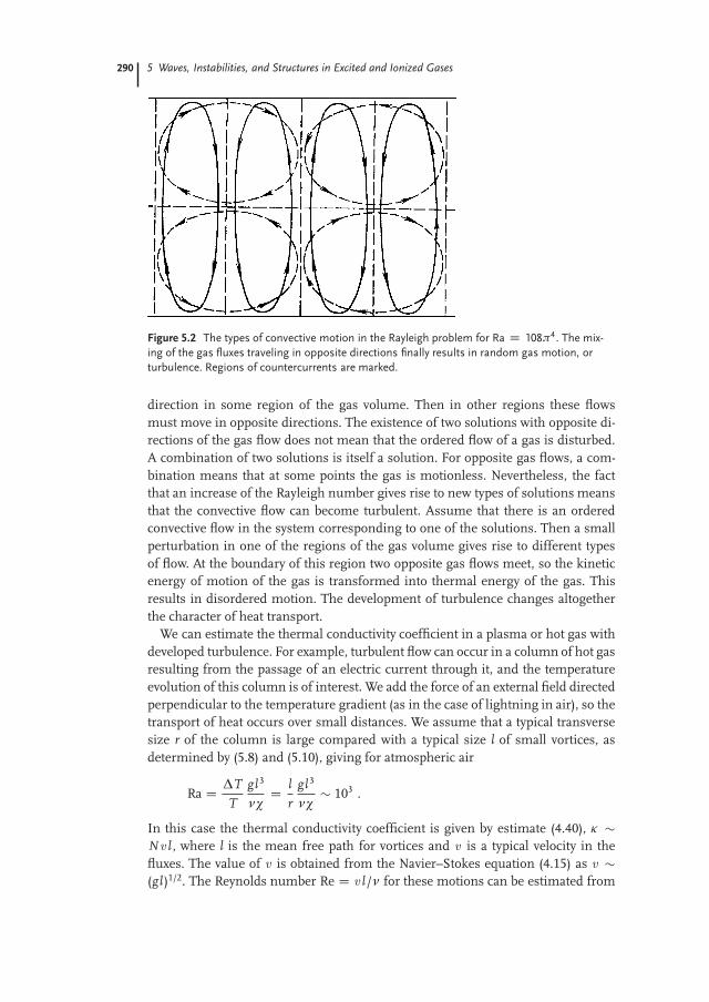
Figure 5.2 shows two types of convective motion for the Rayleigh number Ra D108π4 corresponding to the wave number k1 D 9.4/L for n D 1 and to k2 D 4.7/Lfor n D 2. To analyze this example using these parameters, we combine the solu-tions so that the gas flows corresponding to n D 1 and to n D 2 travel in the same
290 5 Waves, Instabilities, and Structures in Excited and Ionized Gases
Figure 5.2 The types of convective motion in the Rayleigh problem for Ra D 108π4. The mix-
ing of the gas fluxes traveling in opposite directions finally results in random gas motion, or
turbulence. Regions of countercurrents are marked.
direction in some region of the gas volume. Then in other regions these flowsmust move in opposite directions. The existence of two solutions with opposite di-rections of the gas flow does not mean that the ordered flow of a gas is disturbed.A combination of two solutions is itself a solution. For opposite gas flows, a com-bination means that at some points the gas is motionless. Nevertheless, the factthat an increase of the Rayleigh number gives rise to new types of solutions meansthat the convective flow can become turbulent. Assume that there is an orderedconvective flow in the system corresponding to one of the solutions. Then a smallperturbation in one of the regions of the gas volume gives rise to different typesof flow. At the boundary of this region two opposite gas flows meet, so the kineticenergy of motion of the gas is transformed into thermal energy of the gas. Thisresults in disordered motion. The development of turbulence changes altogetherthe character of heat transport.
We can estimate the thermal conductivity coefficient in a plasma or hot gas withdeveloped turbulence. For example, turbulent flow can occur in a column of hot gasresulting from the passage of an electric current through it, and the temperatureevolution of this column is of interest. We add the force of an external field directedperpendicular to the temperature gradient (as in the case of lightning in air), so thetransport of heat occurs over small distances. We assume that a typical transversesize r of the column is large compared with a typical size l of small vortices, asdetermined by (5.8) and (5.10), giving for atmospheric air
Ra D ΔTT
gl3
ν�D l
rg l3
� 103 .
In this case the thermal conductivity coefficient is given by estimate (4.40), � �Nv l , where l is the mean free path for vortices and v is a typical velocity in thefluxes. The value of v is obtained from the Navier–Stokes equation (4.15) as v �(g l)1/2. The Reynolds number Re D v l/ν for these motions can be estimated from

5.1 Instabilities of Excited Gases 291
the above expression for the Rayleigh number, yielding
Ra D lr
ν�
Re2 � 103 .
Since l � r and ν � �, it follows that Re � 1. Thus, at large values of the Rayleighnumber when several types of motion of gaseous flows are possible, the movementof the gas is characterized by large values of the Reynolds number. As these valuesincrease, the gas motion tends toward disorder, and turbulent motion develops.
5.1.6
Thermal Explosion
We shall now consider the other type of instability of a motionless gas, which iscalled thermal instability or thermal explosion. It occurs in a gas experiencing heattransport by way of thermal conduction, where the heat release is determined byprocesses (e.g., chemical) whose rate depends strongly on the temperature. Thereis a limiting temperature where heat release is so rapid that thermal conductivityprocesses cannot transport the heat released, and then an instability occurs, whichis the thermal explosion [13, 14]. As a result of this instability, the internal energy ofthe system is transformed into heat, which leads to a new regime of heat transport.We use the Zeldovich approach [15, 16] in the analysis of this problem.
We shall analyze this instability within the framework of the geometry of theRayleigh problem. Gas is located in a gap between two infinite plates with a dis-tance L between them. The wall temperature is Tw. We take the z-axis as perpen-dicular to the walls, with z D 0 in the middle of the gap, so the coordinates of wallsare z D ˙L/2. We introduce the specific power of heat release f (T ) as the powerper unit volume and use the Arrhenius law [17],
f (T ) D A exp�
� Ea
T
�, (5.19)
for the temperature dependence of this value, where Ea is the activation energy ofthe heat release process. This dependence of the rate of heat release is identicalto that for the chemical process and represents a strong temperature dependencebecause Ea � T . This dependence is used widely for chemical processes [18, 19].
To find the temperature distribution inside a gap in the absence of the thermalinstability, we note that (4.41) for the transport of heat has the form
�d2Tdz2
C f (T ) D 0 .
We introduce a new variable X D Ea(T � T0)/T 20 , where T0 is the gas temperature
in the center of the gap, and obtain the equation
d2 Xdz2 � B exp(�X ) D 0 ,

292 5 Waves, Instabilities, and Structures in Excited and Ionized Gases
where B D EaA exp(�Ea/T0)/(T 20 �). Solving this equation with the boundary con-
ditions X(0) D 0, d X(0)/dz D 0 (the second condition follows from the symmetryX(z) D X(�z) in this problem), we have
X D 2 ln cosh z .
The temperature difference between the center of the gap and the walls is
ΔT � T0 � Tw D 2T 20
Ealn cosh
"L2
sAEa
2T 20 �
exp�
� Ea
2T0
�#. (5.20)
To analyze this expression, we refer to Figure 5.3, illustrating the dependence onT0 for the left-hand and right-hand sides of this equation (curves 1 and 2, respec-tively) at a given Tw. The intersection of these curves yields the center temperatureT0. The right-hand side of the equation does not depend on the temperature of thewalls and depends strongly on T0. Therefore, it is possible that curves 1 and 2 donot intersect. That would mean there is not a stationary solution of the problem.The physical implication of this result is that thermal conduction cannot suffice toremove the heat released inside the gas. This leads to a continuing increase of thetemperature, and thermal instability occurs.
To find the threshold of the thermal instability corresponding to curve 10 in Fig-ure 5.3, we establish the common tangency point of the curves describing the left-hand and right-hand sides of (5.20). The derivatives of the two sides are equal when
ΔT D 2T 20
Ealn cosh y , 1 D y tanh y , (5.21)
where
y D L2
sAEa
2T 20 �
exp�
� Ea
2T0
�.
Figure 5.3 The dependence for the right-hand and left-hand sides of (5.20) on the temperature
in the center. The wall temperature T �w corresponds to the threshold of the thermal instability.

5.1 Instabilities of Excited Gases 293
The solution of the second equation in (5.21) is y D 1.2, so
AEaL2
T 20 �
exp�
� Ea
T0
�D 11.5 , ΔT D 1.19
T 20
Ea. (5.22)
From this, it follows that the connection between the specific powers of heat releaseis
f (Tw) D f (T0) exp �1.19 D 0.30 f (T0) .
This gives the following connection between the parameters for heat release at thewalls at the threshold of thermal instability:
L2AEa
T 2w�
exp�
� Ea
Tw
�D 3.5 . (5.23)
Although we referred to the Arrhenius law for the temperature dependence of therate of heat release, in actuality we used only the implication that this dependenceis strong. We can, therefore, rewrite the condition for the threshold of the thermalinstability in the form
L2
�
ˇ̌̌ˇ d f (Tw)
dTw
ˇ̌̌ˇ D 3.5 . (5.24)
The criterion for a sharp peak in the power involved in the heat release is
Tw
ˇ̌̌ˇ d f (Tw)
dTw
ˇ̌̌ˇ � 1 . (5.25)
Relation (5.24) has a simple physical meaning. It relates the rate of the heat re-lease process to the rate of heat transport. If their ratio exceeds a particular value ofthe order of unity, then thermal instability develops.
5.1.7
Thermal Waves
The development of thermal instability can lead to the formation of a thermal wave.This takes place if the energy in some internal degree of freedom is significantly inexcess of its equilibrium value. It can occur in a chemically active gas in combus-tion processes, and the theory of propagation of thermal waves [20–23] used belowwas developed for these processes. But the thermal explosion that is accompaniedby propagation of a thermal wave has a universal character and may be employedalso for problems involving ionized gases. Below we will be guided by a thermalwave propagating in a nonequilibrium molecular gas where the vibration temper-ature exceeds significantly the gas translation temperature, as occurs in moleculargas lasers, in particular, CO2 and CO gas lasers. In these cases the development ofthermal instability leads to a vibrational relaxation that is accompanied by equaliz-ing of the translational and vibrational temperatures and proceeds in the form of apropagating thermal wave. Below we will be guided by this problem.

294 5 Waves, Instabilities, and Structures in Excited and Ionized Gases
Figure 5.4 The temperature distribution in a gas in which a thermal wave propagates.
Figure 5.4 shows the temperature distribution in a gas upon propagation of athermal wave. Region 1 has the initial gas temperature. The wave has not yetreached this region at the time represented in the figure. The temperature riseobserved in region 2 is due to heat transport from hotter regions. The temperaturein region 3 is close to the maximum. Processes that release heat occur in this re-gion. We use the strong temperature dependence to establish the specific power ofheat release, which according to (5.19) has the form
f (T ) D f (Tm) exp��α(Tm � T )
, α D Ea
T 2m
. (5.26)
Here Tm is the final gas temperature, determined by the internal energy of the gas.Region 4 in Figure 5.4 is located after the passage of the thermal wave. Thermody-namic equilibrium among the relevant degrees of freedom has been established inthis region.
To calculate the parameters of the thermal wave, we assume the usual connectionbetween spatial coordinates and the time dependence of propagating waves. Thatis, the temperature is taken to have the functional dependence T D T(x � ut),where x is the direction of wave propagation and u is the velocity of the thermalwave. With this functional form, the heat balance equation (4.41) becomes
udTdx
C �d2 Tdx2
C f (T )c p N
D 0 . (5.27)
Our goal is to determine the eigenvalue u of this equation. To accomplish this, weemploy the Zeldovich approximation method [15, 16], which uses a sharply peakedtemperature dependence for the rate of heat release. We introduce the functionZ(T ) D �dT/dx , so for T0 < T < Tm we have Z(T ) � 0. Because of the equation
d2Tdx2 D d
dx
�dTdx
�D Z dZ
dT,
equation (5.27) takes the form
�uZ C �Z dZdT
C f (T )c p N
D 0 . (5.28)

5.1 Instabilities of Excited Gases 295
Figure 5.5 The solution of (5.28) for various regions of the thermal wave giving rise to Fig-
ure 5.4.
The solution of this equation for the regions defined in Figure 5.4 is illustratedin Figure 5.5. Before the thermal wave (region 1) and after it (region 4), we haveZ D 0. In region 2 there is no heat release, and one can ignore the last termin (5.28). This yields
Z D u(T � T0)�
. (5.29)
Ignoring the first term in (5.28), we obtain
Z D
vuuut 2c p N �
TmZT
f (T )dT (5.30)
for region 3 in Figure 5.5. Equations (5.29) and (5.30) are not strictly joined at theinterface between regions 2 and 3 because there is no interval where one can ignoreboth terms in (5.28). But because of the very strong dependence of f (T ) on T, thereis only a narrow temperature region where it is impossible to ignore one of theseterms. This fact allows us to connect solution (5.29) with (5.30) and find the velocityof the thermal wave.
Introducing the temperature T� that corresponds to the maximum of Z(T ),(5.28) gives
Zmax D Z(T�) D f (T�)uc p N
.
Equation (5.28) for temperatures near T� then takes the form
dZdT
D u�
�1 � f (T )
f (T�)
�.
Solving this equation and taking into account (5.26), we have
Z D u�
(T � T0) � u�α
exp[α(T � T�)] . (5.31)

296 5 Waves, Instabilities, and Structures in Excited and Ionized Gases
The boundary condition for this equation is that it should coincide with (5.29) farfrom the maximum Z. In this region one can ignore the third term in (5.28), whichis the approximation that leads to (5.29). This is valid under the condition
α(T� � T0) � 1 . (5.32)
Now we seek the solution of (5.28) at T > T�. Near the maximum of Z(T ), Z isgiven by (5.31), so (5.28) has the form
dZdT
D Zmax
T� � T0f1 � exp[α(T � T�)]g .
This equation is valid in the region where the second term in (5.31) is significantlysmaller than the first one. According to condition (5.32), this condition is fulfilledat temperatures where exp[α(T � T�)] � 1. Therefore, because of the exponentialdependence of the second term in (5.28), there is a temperature region where thesecond term in (5.28) gives a scant contribution to Z, but nevertheless determinesits derivative. This property will be used below. On the basis of the above infor-mation and the dependence given in (5.26), we find that the solutions of (5.28) atT > T� are
Z Ds
2 f (Tm)c p N �α
p1 � exp[α(T � Tm)] ,
dZdT
Ds
2 f (Tm)c p N �α
exp[α(T � Tm)]p1 � exp[α(T � Tm)]
.
Comparing the expressions for dZ/dT near the maximum, one can see thatthey can be connected if condition (5.32) is satisfied. Then solution (5.30) is validin the temperature region T� < T Tm up to temperatures near the maximumof Z. Connecting values of dZ/dT in regions where α(T � T�) � 1 and whereα(Tm � T ) � 1, we obtain
Zmax Ds
2 f (Tm)c p N �α
(T� � Tm) exp[α(T� � Tm)] .
Next, from (5.31) it follows that Zmax D Z(T�) D f (T�)/(uc p N ). Comparing theseexpressions, one can find the temperature T� corresponding to the maximum ofZ(T ) and hence to the velocity of the thermal wave. We obtain
α(T� � T0)2
D exp[α(Tm � T�)] , (5.33)
u D Tm
Tm � T0
s2� f (Tm)c p N Ea
. (5.34)
We used (5.26) for α. Relation (5.33) together with condition (5.32) gives Tm�T� �T� � T0. This was taken into account in (5.32).

5.1 Instabilities of Excited Gases 297
Formula (5.34) corresponds to the dependence (5.26) for the rate of heat re-lease near the maximum. In a typical case at T D Tm all the “fuel” is used, andf (Tm) D 0. Then all the above arguments are valid, because the primary portion
of the heat release takes place at temperatures T, where α(Tm � T ) � 1, that is,where α(T � T�) � 1. Then, using the new form of the function f (T ) near themaximum of Z(T ), we transform (5.34) for the velocity of the thermal wave intothe form
u D 1Tm � T0
vuuut 2�c p N
TmZT
f (T )dT . (5.35)
This formula is called the Zeldovich formula.We can analyze the problem from another standpoint. We take an expression for
Z(T ) such that, in the appropriate limits, it would agree with (5.29) and (5.30). Thesimplest expression of this type has the form
Z D u�
(T � T0) f1 � exp[�α(Tm � T )]g .
If we insert this into (5.28), f (T ) is given by
f (T )c p N
D uZ � �2
ddT
Z2 D u2
�(T � T0)
p1 � exp �α(Tm � T )
h1 �p
1 � exp(�α(Tm � T ))i
C αu2
2�(T � T0)2 exp[�α(Tm � T )] .
In the region α(T � T0) � 1, the first term is small compared with the second oneand one can ignore it. Then the comparison of this expression with that in (5.26) inthe temperature region α(Tm � T ) � 1 and Tm � T � Tm � T0 gives the velocityof the thermal wave as
u D Tm
Tm � T0
s2�Ea
f (Tm)c p N
.
where α D Ea/T 2m. This equation agrees exactly with (5.34) because of the identical
assumptions used for construction of the solution in both cases.One can use this method for the alternative case when the function f (T ) has an
exponential dependence far from Tm, and goes to zero at T D Tm. For example,we take the approximate dependence
f (T ) D A(Tm � T ) exp[�α(Tm � T )] .
An approximate solution of (5.28) constructed on the basis of (5.29) and (5.30) hasthe form
Z D u�
(T � T0)q
1 � e�α(Tm�T )[α(Tm � T ) C 1] .

298 5 Waves, Instabilities, and Structures in Excited and Ionized Gases
Substituting this into (5.28), we have
f (T )c p N
D uZ � �2
dZ2
dTD u2
�(T � T0)
p1 � e�α(Tm�T )
h1 �
p1 � e�α(Tm�T )
iC αu2
2�(T � T0)2e�α(Tm�T ) .
In the region α(T � T0) � 1, where the heat release is essential, the first term issmall compared with the second one. Then comparing this expression with the ap-proximate dependence assumed above for f (T ), we find the velocity of the thermalwave α D Ea/T 2
m to be
u D T 2m
Ea(Tm � T0)
s2�Ac p N
.
This result is in agreement with the Zeldovich formula (5.35) for the dependenceemployed for f (T ). The above analysis shows that the Zeldovich formula for thevelocity of a thermal wave is valid under the condition α(Tm � T0) � 1.
5.1.8
Thermal Waves of Vibrational Relaxation
We shall apply the above results to the analysis of illustrative physical processes.First we consider a thermal wave of vibrational relaxation that can propagate in anexcited molecular gas that is not in equilibrium. In particular, this process can oc-cur in molecular lasers, where it can result in the quenching of laser generation. Weconsider the case where the number density of excited molecules is considerablygreater than the equilibrium density. Vibrational relaxation of excited moleculescauses the gas temperature to increase and the relaxation process accelerates. Therewill be a level of excitation and a temperature at which thermal instability develops,leading to the establishment of a new thermodynamic equilibrium between excitedand nonexcited molecules.
The balance equation for the number density of excited molecules N� has theform
@N�
@tD DΔN� � N N�k(T ) ,
where N is the total number density of molecules, and where we assume N � N�.D is the diffusion coefficient for excited molecules in a gas, and k(T ) is the rateconstant for vibrational relaxation. Taking into account the usual dependence oftraveling wave parameters N�(x , t) D N�(x � ut), where u is the velocity of thethermal wave, we transform the above equation into the form
udN�
dxC D
d2 N�
dx2 � N�N k(T ) D 0 . (5.36)
In front of the thermal wave we have N� D Nmax, and after the wave we haveN� D 0. That is, we are assuming the equilibrium number density of excited
5.1 Instabilities of Excited Gases 299
molecules to be small compared with the initial density. We introduce the meanenergy Δε released in a single vibrational relaxation event. Then the differencebetween the gas temperatures after Tm and before T0 the thermal relaxation waveis
Tm � T0 D N0ΔεN c p
,
where N0 is the initial number density of excited molecules.The heat balance equation (5.27) now has the form
udTdx
C �d2Tdx2 � ΔεN�k(T )
c pD 0 . (5.37)
The wave velocity can be obtained from the simultaneous analysis of (5.36) and(5.37). The simplest case occurs when D D �. Then, both balance equations areidentical, and the relation between the gas temperature and the number density ofexcited molecules is
Tm � T D N�ΔεN c p
. (5.38)
We have only one balance equation in this case. Comparing it with (5.27), we havef (T )/(c p N ) D (Tm � T )N k(T ). On the basis of the Zeldovich formula we find the
wave velocity to be
u D T 2m
Ea(Tm � T0)
s2�
τ(Tm), (5.39)
where τ(Tm) D 1/[N k(Tm)] is a typical time for vibrational relaxation at tempera-ture Tm. Because of the assumption α(Tm � T0) � 1 and the dependence (5.26)for the rate constant for vibrational relaxation, relation (5.39) with the assumptionsemployed gives
u �r
�τ(Tm)
.
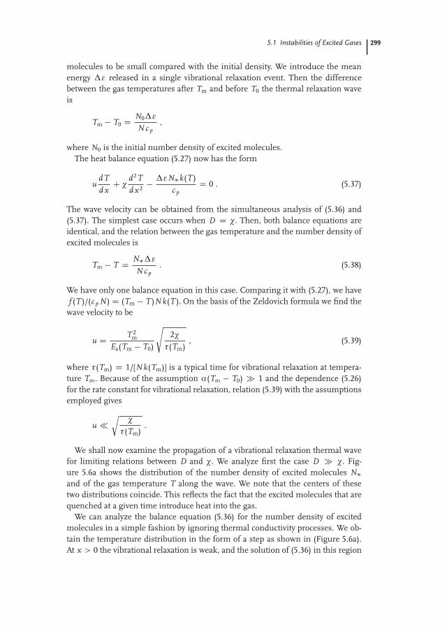
We shall now examine the propagation of a vibrational relaxation thermal wavefor limiting relations between D and �. We analyze first the case D � �. Fig-ure 5.6a shows the distribution of the number density of excited molecules N�
and of the gas temperature T along the wave. We note that the centers of thesetwo distributions coincide. This reflects the fact that the excited molecules that arequenched at a given time introduce heat into the gas.
We can analyze the balance equation (5.36) for the number density of excitedmolecules in a simple fashion by ignoring thermal conductivity processes. We ob-tain the temperature distribution in the form of a step as shown in (Figure 5.6a).At x > 0 the vibrational relaxation is weak, and the solution of (5.36) in this region

300 5 Waves, Instabilities, and Structures in Excited and Ionized Gases
Figure 5.6 The distribution of the gas tem-
perature and the number density of excit-
ed molecules in the thermal wave of vibra-
tional relaxation for different limiting ratios
between the diffusion coefficient of excited
molecules D and the thermal diffusivity coeffi-
cient � of the gas: (a) D � � and (b) � � D
has the form N� D Nmax � (Nmax � N0) exp(�ux/D) if x > 0, where N0 is the num-ber density of the excited molecules at x D 0 and N0 is the integration constant. Inthe region x < 0 vibrational relaxation is of importance, but the gas temperatureis constant. This leads to
N� D N0 exp(αx ) , x < 0 , α Dr� u
2D
�2 C 1D τ
� u2D
,
where τ D 1/[N k(Tm)]. The transition region, where the gas temperature is notat its maximum, but the vibrational relaxation is essential, is narrow under theconditions considered. Hence, at x D 0 the above expressions must give the sameresults both for the number density of excited molecules and for their derivatives.We obtain
α D uD
, u Dr
2DτT
D p2D N k(Tm) , D � � . (5.40)
In this case the propagation of the thermal wave of vibrational relaxation is gov-erned by the diffusion of excited molecules in a hot region where vibrational re-laxation takes place. Hence, the wave velocity is of the order of u � p
D/τ inaccordance with (5.40). The width of the front of the thermal wave is estimated asΔx � p
D τ.
5.1 Instabilities of Excited Gases 301
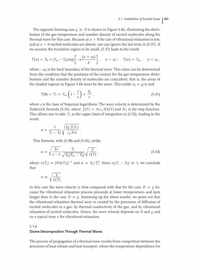
The opposite limiting case � � D is shown in Figure 5.6b, illustrating the distri-bution of the gas temperature and number density of excited molecules along thethermal wave for this case. Because at x > 0 the rate of vibrational relaxation is low,and at x < 0 excited molecules are absent, one can ignore the last term in (5.37). Ifwe assume the transition region to be small, (5.37) leads to the result
T(x ) D T0 C (Tm � T0) exp��u
(x C x0)�
�, x > x0 I T(x ) D Tm , x < x0 ,
where �x0 is the back boundary of the thermal wave. This value can be determinedfrom the condition that the positions of the centers for the gas temperature distri-butions and the number density of molecules are coincident; that is, the areas ofthe shaded regions in Figure 5.6b must be the same. This yields x0 D �/u and
T(0) D Tr D Tm
�1 � 1
e
�C T0
e, (5.41)
where e is the base of Naperian logarithms. The wave velocity is determined by theZeldovich formula (5.35), where f (T ) D Δε�N k(T ) and N� is the step function.This allows one to take Tr as the upper limit of integration in (5.35), leading to theresult
u D 1Tr � T0
s2� f (Tr )c p N α
.
This formula, with (5.38) and (5.41), yields
u Dr
2ee � 1
TrpEa(Tm � T0)
r�
τ(T ), (5.42)
where τ(Tr) D [N k(Tr )]�1 and α D Ea/T 2r . Since α(Tr � T0) � 1, we conclude
that
u �r
�k(T )
.
In this case the wave velocity is slow compared with that for the case D D � be-cause the vibrational relaxation process proceeds at lower temperatures and lastslonger than in the case D D �. Summing up the above results, we point out thatthe vibrational relaxation thermal wave is created by the processes of diffusion ofexcited molecules in a gas, by thermal conductivity of the gas, and by vibrationalrelaxation of excited molecules. Hence, the wave velocity depends on D and � andon a typical time τ for vibrational relaxation.
5.1.9
Ozone Decomposition Through Thermal Waves
The process of propagation of a thermal wave results from competition between theprocesses of heat release and heat transport, where the temperature dependence for

302 5 Waves, Instabilities, and Structures in Excited and Ionized Gases
the heat release is sharper than for heat transport. This character of heat processesis of universal character and may be applied to some processes in ionized gases.We considered above a thermal wave of vibrational relaxation in a nonequilibriummolecular gas, and below we consider one more process of this type, which resultsin decomposition of ozone in air or other gases and proceeds in the form of a ther-mal wave. The propagation of the thermal wave results from chemical processeswhose basic stages are
O3 CMkdis! O2 COCM , OCO2 CM
K! O3 CM , OCO3k1! 2O2 (5.43)
where M is a gas molecule and the relevant rate constants for the processes aregiven above the arrows. If these processes proceed in air, the temperature Tm afterthe thermal wave is connected to the initial gas temperature T0 by
Tm D T0 C 48c , (5.44)
where the temperatures are expressed in Kelvin and c is the ozone concentrationin air expressed as a percentage.
On the basis of scheme (5.43), we obtain the set of balance equations
d[O3]d t
D �kdis[M][O3] C K [O][O2][M] � k1[O][O3] ,
d[O]d t
D kdis[M][O3] � K [O][O2][M] � k1[O][O3] , (5.45)
where [X] is the number density of particles X. Estimates show that at gas pressurep 1 atm and Tm > 500 K we have K [O2][M] � k1[O3], that is, the second termon the right-hand side of each equation in (5.45) is smaller than the third one.In addition, we know that [O] � [O3], that is, d[O]/d t � d[O3]/d t. This givesd[O]/d t D 0 and [O] D kdis[M]/ k1. Using this result in the first equation in (5.45),we obtain
d[O3]d t
D �2kdis[M][O3] .
Then, with (5.36) and (5.37), we obtain for the thermal wave
ud[O3]dx
C Dd2[O3]dx2
� 2kdis[M][O3] D 0 ,
udTdx
C �d2Tdx2 C 2
c pΔεkdis[O3] D 0 , (5.46)
where Δε D 1.5 eV is the energy released from the decomposition of one ozonemolecule.
We can now substitute numerical parameters of the above processes for athermal wave in air at atmospheric pressure, namely, D D 0.16 cm2/s and� D 0.22 cm2/s. These quantities are almost equal numerically and have simi-lar temperature dependence, so we take them to be equal and given by
D D � D 0.19p
�T
300
�1.78
.

5.1 Instabilities of Excited Gases 303
Figure 5.7 The velocity of the thermal wave of ozone decomposition (u) and the width of the
wave front (Δx) as a function of the final temperature.
Here D and � are expressed in square centimeters per second, the air pressure pis given in atmospheres, and the temperature is expressed in Kelvin. Next, weemploy the expression kdis D 1.0 10�9 cm3/s exp(�11 600/T ) for the dissocia-tion rate constant. We can observe how equating D and � simplifies the problem.Then (5.39) gives the thermal wave velocity
u D 1.3T 2.39m
Tm � T0exp
�� 5800
Tm
�,
where the initial (T0) and final (Tm) air temperatures are expressed in Kelvin, andthe thermal wave velocity is in centimeters per second. Figure 5.7 illustrates thetemperature dependence for the wave velocity with T0 D 300 K. Note that it doesnot depend on the air pressure.
The width of the wave front can be characterized by the Δx D (Tm � T0)/(dT/dx )max, where the maximum temperature gradient is (dT/dx )max Du(T� � T0)/� and the temperature T� is determined by (5.33). Figure 5.7 givesthis value as a function of the temperature. From the data in Figure 5.7, one cansee that the thermal wave velocity is small compared with the sound velocity. Thismeans that the propagation of a thermal wave is a slow process in contrast to thatfor a shock wave.

304 5 Waves, Instabilities, and Structures in Excited and Ionized Gases
5.2
Waves in Ionized Gases
5.2.1
Acoustic Oscillations
Oscillations and noise in a plasma play a much greater role than in an ordinarygas because of the long-range nature of charged particle interactions. If a plasmais not uniform and is subjected to external fields, a wide variety of oscillations canoccur [24, 25]. Under some conditions, these oscillations can become greatly ampli-fied. Then the plasma oscillations affect basic plasma parameters and properties.Below we analyze the simplest types of oscillations in a gas and in a plasma. Thenatural vibrations of a gas are acoustic vibrations, that is, waves of alternating com-pressions and rarefactions that propagate in gases. We shall analyze these waveswith the goal of finding the relationship between the frequency ω of the oscillationand the wavelength λ, which is connected to the wave vector k by jkj D 2π/λ. It iscustomary to refer to the amplitude k D jkj as the wave number.
In our analysis, we assume the oscillation amplitudes to be small. Thus, anymacroscopic parameter of the system can be expressed as
A D A 0 CX
ω
A0ω exp[i(k x � ω t)] , (5.47)
where A 0 is an unperturbed parameter (in the absence of oscillations), A0ω is the
amplitude of the oscillations, ω is the oscillation frequency, and k is the appro-priate wave number. The wave propagates along the x-axis. Since the oscillationamplitude is small, an oscillation of a given frequency does not depend on oscilla-tions with other frequencies. In other words, there is no coupling between wavesof different frequencies when the amplitudes are small. Therefore, one need retainonly the leading term in sum (5.47) and can express the macroscopic parameter Ain the form
A D A 0 C A0 exp[i(kx � ω t)] . (5.48)
To analyze acoustic oscillations in a gas, we can apply (5.48) to the number den-sity of gas atoms (or molecules) N, the gas pressure p, and the mean gas velocity w,and take the unperturbed gas to be at rest (w0 D 0). Using the continuity equa-tion (4.1) and ignoring terms with squared oscillation amplitudes, we obtain
ωN 0 D kN0w 0 . (5.49)
The gas velocity w is directed along the wave vector k for an acoustic wave (a longi-tudinal oscillation). Similarly, the Euler equation (4.15) in the linear approximationleads to
ωw 0 D kmN0
p 0 , (5.50)
where m is the mass of the particles of the gas.
5.2 Waves in Ionized Gases 305
Equations (5.49) and (5.50) connect the oscillation frequency ω and the wavenumber by the relation
ω D csk , (5.51)
where the speed of sound cs is
cs Dr
p 0
mN 0Dr
1m
@p@N
. (5.52)
An equation of the type of (5.51) that connects the frequency ω of the wave with itswave number k is called a dispersion relation. We see that here the group velocityof sound propagation @ω/@k is the same as the phase velocity ω/ k and does notdepend on the sound frequency.
To find the sound velocity, it is necessary to know the connection between vari-ations of the gas pressure and density in the acoustic wave. For long waves, theregions of compression and rarefaction do not exchange energy during wave prop-agation. Hence, this process is adiabatic, and the parameters of the acoustic wavesatisfy the adiabatic equation
p N�γ D const , (5.53)
where γ D c p /cV is the adiabatic exponent. That is, c p is the specific heat capacityat constant pressure, and cV is the specific heat capacity at constant volume. Onthe basis of expansion (5.48), the wave parameters are related by
p 0
p0D γ
N 0
N0.
Because of the state equation (4.11), p D N T , where T is the gas temperature, weobtain p 0/N 0 D @p/@N D γ T . Thus, the dispersion relation (5.51) yields
ω Dr
γ Tm
k . (5.54)
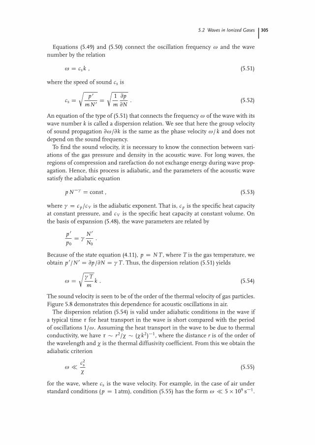
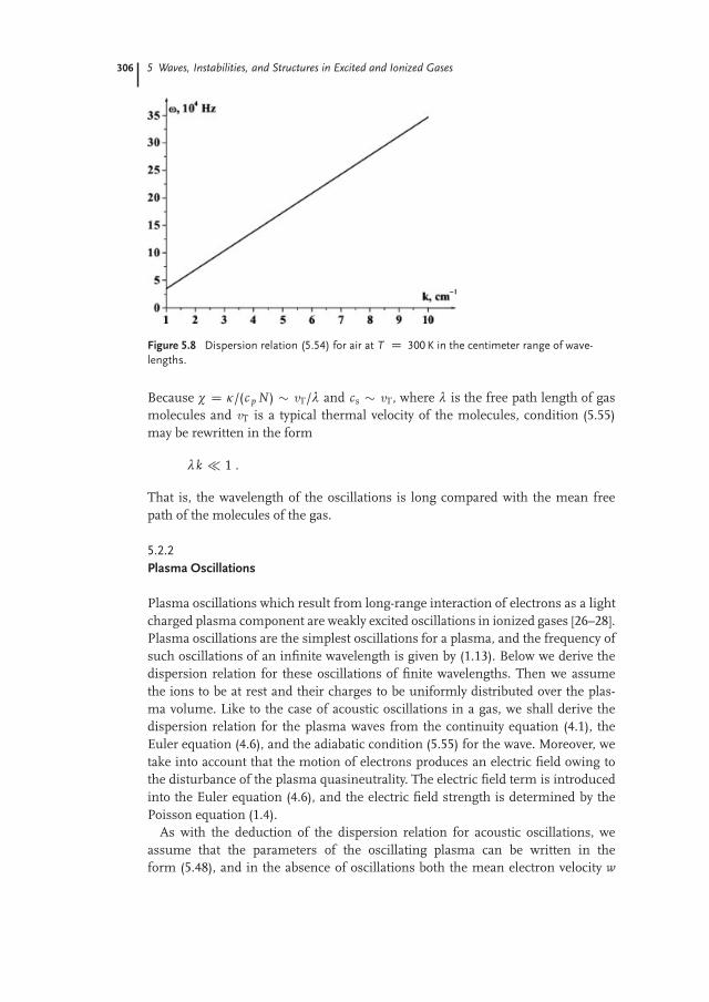
The sound velocity is seen to be of the order of the thermal velocity of gas particles.Figure 5.8 demonstrates this dependence for acoustic oscillations in air.
The dispersion relation (5.54) is valid under adiabatic conditions in the wave ifa typical time τ for heat transport in the wave is short compared with the periodof oscillations 1/ω. Assuming the heat transport in the wave to be due to thermalconductivity, we have τ � r2/� � (�k2)�1, where the distance r is of the order ofthe wavelength and � is the thermal diffusivity coefficient. From this we obtain theadiabatic criterion
ω � c2s
�(5.55)
for the wave, where cs is the wave velocity. For example, in the case of air understandard conditions (p D 1 atm), condition (5.55) has the form ω � 5 109 s�1.
306 5 Waves, Instabilities, and Structures in Excited and Ionized Gases
Figure 5.8 Dispersion relation (5.54) for air at T D 300 K in the centimeter range of wave-
lengths.
Because � D �/(c p N ) � vT/λ and cs � vT, where λ is the free path length of gasmolecules and vT is a typical thermal velocity of the molecules, condition (5.55)may be rewritten in the form
λk � 1 .
That is, the wavelength of the oscillations is long compared with the mean freepath of the molecules of the gas.
5.2.2
Plasma Oscillations
Plasma oscillations which result from long-range interaction of electrons as a lightcharged plasma component are weakly excited oscillations in ionized gases [26–28].Plasma oscillations are the simplest oscillations for a plasma, and the frequency ofsuch oscillations of an infinite wavelength is given by (1.13). Below we derive thedispersion relation for these oscillations of finite wavelengths. Then we assumethe ions to be at rest and their charges to be uniformly distributed over the plas-ma volume. Like to the case of acoustic oscillations in a gas, we shall derive thedispersion relation for the plasma waves from the continuity equation (4.1), theEuler equation (4.6), and the adiabatic condition (5.55) for the wave. Moreover, wetake into account that the motion of electrons produces an electric field owing tothe disturbance of the plasma quasineutrality. The electric field term is introducedinto the Euler equation (4.6), and the electric field strength is determined by thePoisson equation (1.4).
As with the deduction of the dispersion relation for acoustic oscillations, weassume that the parameters of the oscillating plasma can be written in theform (5.48), and in the absence of oscillations both the mean electron velocity w

5.2 Waves in Ionized Gases 307
and the electric field strength E are zero. Hence, we obtain
� i ωN 0e C i kN0w 0 D 0 , �i ωw 0 C i
k p 0
meN0C eE 0
meD 0 ,
p 0
p0D γ
N 0e
N0, i kE 0 D �4πeN . (5.56)
Here k and ω are the wave number and the frequency of the plasma oscillations, N0
is the mean number density of charged particles, p0 D N0me˝v2
x
˛is the electron gas
pressure in the absence of oscillations, me is the electron mass, vx is the electronvelocity component in the direction of oscillations, and the angle brackets denoteaveraging over electron velocities. N 0
e, w 0, p 0, and E 0 in (5.56) are the oscillationamplitudes for the electron number density, mean velocity, pressure, and electricfield strength, respectively.
Eliminating the oscillation amplitudes from the system of equations in (5.56),we obtain the dispersion relation for plasma oscillations;
ω2 D ω2p C γ
˝v2
x
˛k2 , (5.57)
where ωp D p4πN0e2/me is the plasma frequency defined by (1.13). Plasma os-
cillations or Langmuir oscillations are longitudinal, in contrast to electromagneticoscillations. Hence, the electric field due to plasma waves is directed along the wavevector. This fact was used in deducing the set of equations in (5.56).
The dispersion relation (5.57) is valid for adiabatic propagation of plasma oscil-lations. If heat transport is due to thermal conductivity of electrons, the adiabaticcondition takes the form ωτ � ω/(�k2) � 1 (compare this with criterion (5.55)),where ω is the frequency of oscillations, τ � (�k2)�1 is a typical time for heattransport in the wave, � is the electron thermal diffusion coefficient, and k is thewave number of the wave. Since � � ve λ, ω � ωp � ve/rD, where ve is the meanelectron velocity, λ is the electron mean free path, and rD is the Debye–Hückelradius given by (1.9). The adiabatic condition yields
λrD k2 � 1 .
If this inequality is reversed, then isothermal conditions in the wave are fulfilled.In this case the adiabatic parameter γ in the dispersion relation (5.57) must bereplaced by the coefficient 3/2 since for the pressure we use the equation of thegaseous state, p D N/T . As a result, we have in the isothermal case the followingdispersion relation for plasma oscillations instead of (5.57) [29, 30]:
ω2 D ω2p C 3k2 Te
me. (5.58)
Note that because the frequency of plasma oscillations is much greater than theinverse of a typical time interval between electron–atom collisions, we have ωp �Nave σea � ve/λ. From this it follows that λ � rD.

308 5 Waves, Instabilities, and Structures in Excited and Ionized Gases
5.2.3
Ion Sound
Since an ionized gas contains two types of charged particles, electrons and ions,there are two types of plasma oscillations due to electrons and ions [28]. Abovewe considered fast oscillations, in which ions as a slow plasma component do notpartake, and now we analyze the oscillations due to the motion of ions in a homo-geneous plasma. The special character of these oscillations is due to the large massof ions. This stands in contrast to the small mass of electrons that enables them tofollow the plasma field, so the plasma remains quasineutral on average:
Ne D Ni .
Moreover, the electrons have time to redistribute themselves in response to theelectric field in the plasma. Then the Boltzmann equilibrium is established, andthe electron number density is given by the Boltzmann formula (1.43):
Ne D N0 exp�
e'
Te
�� N0
�1 C e'
Te
�,
where ' is the electric potential due to the oscillations and Te is the electron tem-perature. These properties of the electron oscillations allows us to express the am-plitude of oscillations of the ion number density as
N 0i D N0
e'
Te. (5.59)
We can now introduce the equation of motion for ions. The continuity equa-tion (4.1) has the form @Ni/@t C @(Niwi)/@x D 0 and gives
ωN 0i D kN0wi , (5.60)
where ω is the frequency, k is the wave number, and wi is the mean ion velocitydue to the oscillations. Here we assume the usual harmonic dependence (5.48) foroscillation parameters. The equation of motion for ions due to the electric field ofthe wave has the form
midwi
d tD eE D �er' .
Taking into account the harmonic dependence (5.48) on the spatial coordinates andtime, we have
miωwi D ek' . (5.61)
Eliminating the oscillation amplitudes of Ni, ', and wi in the set of equa-tions (5.59), (5.60), and (5.61), we obtain the dispersion relation
ω D k
sTe
mi(5.62)

5.2 Waves in Ionized Gases 309
connecting the frequency and wave number. These oscillations caused by ion mo-tion are known as ion sound. As with plasma oscillations, ion sound is a longitudi-nal wave, that is, the wave vector k is parallel to the oscillating electric field vector E.The dispersion relation for ion sound is similar to that for acoustic waves. This isbecause both types of oscillations are characterized by a short-range interaction. Inthe case of ion sound, the interaction is short-ranged because the electric field ofthe propagating wave is shielded by the plasma. This shielding is effective if thewavelength of the ion sound is considerably greater than the Debye–Hückel radiusfor the plasma where the sound propagation occurs, that is, k rD � 1. Dispersionrelation (5.62) is valid if this condition is fulfilled.
To find the dispersion relation for ion sound in a general case, we start with thePoisson equation for the plasma field in the form
d2'
dx2 D 4πe(Ne � Ni) .
In the case of long-wave oscillations treated above, we took the left-hand side of thisequation to be zero. Now, using the harmonic dependence of wave parameters onthe coordinates and time, we obtain �k2' for the left-hand side of this equation.Taking N 0
e D N0(1 C e'/Te) in the right-hand side of this Poisson equation, weobtain
N 0i D N0
e'
Te
�1 C k2Te
4πN0e2
�.
In the treatment of long-wave oscillations, we ignored the second term in the paren-theses. Hence, dispersion relation (5.62) is now replaced by [28]
ω D k
sTe
mi
s1 C k2Te
4πN0e2. (5.63)
This dispersion relation transforms into (5.62) in the limit k rD � 1 when the os-cillations are determined by short-range interactions in the plasma. In the oppositelimit k rD � 1, we get
ω Ds
4πN0e2
mi. (5.64)
In this case a long-range interaction in the plasma is of importance, and from theform of the dispersion relation, we see that ion oscillations are similar to plasmaoscillations.
5.2.4
Magnetohydrodynamic Waves
New types of oscillations arise in a plasma subjected to a magnetic field. We con-sider the simplest oscillations of this type in a high-conductivity plasma. In this

310 5 Waves, Instabilities, and Structures in Excited and Ionized Gases
case the magnetic lines of force are frozen in the plasma [31], and a change inthe plasma current causes a change in the magnetic lines of force, which acts inopposition to this current and creates oscillations of the plasma together with themagnetic field [32–34]. Such oscillations are called magnetohydrodynamic waves.
For magnetohydrodynamic waves with wavelengths less than the radius of cur-vature of the magnetic lines of force, we have
1k
�ˇ̌̌ˇ HrH
ˇ̌̌ˇ , (5.65)
where H is the magnetic field strength. Then one can consider the magnetic linesof force to be straight lines. We construct a simple model of oscillations of a high-conductivity plasma, where the magnetic lines of force are frozen in the plasma.The displacement of the magnetic lines of force causes a plasma displacement,and because of the plasma elasticity, these motions are oscillations. The velocity ofpropagation of this oscillation is, according to dispersion relation (5.52), given byc D p
@p/@�, where p is the pressure, � D M N is the plasma density, and M is theion mass. Because the pressure of a cold plasma is equal to the magnetic pressurep D H2/(8π), we have
c Dr
H@H/@N4πM
for the velocity of wave propagation. Since the magnetic lines of force are frozen inthe plasma, @H/@N D H/N . This gives [32–34]
c D cA D Hp4πM N
(5.66)
for the velocity of these waves. cA is called the Alfvén speed.The oscillations being examined may be of two types depending on the direction
of wave propagation, as shown in Figure 5.9 [35]. If the wave propagates alongthe magnetic lines of force, it is called an Alfvén wave or magnetohydrodynamicwave. This wave is analogous to a wave propagating along an elastic string. Theother wave type propagates perpendicular to the magnetic lines of force. Then thevibration of one magnetic line of force causes the vibration of a neighboring line.Such waves are called magnetic sound. The dispersion relation for both types ofoscillations has the form
ω D cAk .
The oscillations in a magnetic field are of importance for the Sun’s plasma [36].There are various types of waves in a plasma in a magnetic field [37].
5.2.5
Propagation of Electromagnetic Waves in a Plasma
We shall now derive the dispersion relation for an electromagnetic wave propagat-ing in a plasma. Plasma motion due to an electromagnetic field influences the wave

5.2 Waves in Ionized Gases 311
Figure 5.9 Two types of magnetohydrodynamic waves: (a) magnetic sound; (b) Alfvén waves.
parameters, and therefore the plasma behavior establishes the dispersion relationfor the electromagnetic wave. We employ Maxwell’s equations [38, 39] as they wererepresented by Heaviside [40] for the electromagnetic wave:
curl E D � 1c
@H@t
, curl H D 4πc
j � 1c
@E@t
. (5.67)
Here E and H are the electric and magnetic fields in the electromagnetic wave, j isthe density of the electron current produced by the action of the electromagneticwave, and c is the light velocity. Applying the curl operator to the first equationin (5.67) and the operator �(1/c)(@/@t) to the second equation, and then eliminatingthe magnetic field from the resulting equations, we obtain
r div E � ΔE C 4πc2
@j@t
� 1c2
@2E@t2
D 0 .
We assume the plasma to be quasineutral, so div E D 0. The electric current isdue to motion of the electrons, so j D �eN0w, where N0 is the average numberdensity of electrons and w is the electron velocity due to the action of the electro-magnetic field. The equation of motion for the electrons is medw/d t D �eE, whichleads to the relation
@j@t
D �eN0dwd t
D e2N0
meE .
Hence, we obtain
ΔE � ω2p
c2 E C 1c2
@2E@t2 D 0 (5.68)
for the electric field of the electromagnetic wave, where ωp is the plasma frequency.Writing the electric field strength in the form (5.48) and substituting it into theabove equation, we obtain the dispersion relation for the electromagnetic wave [41]:
ω2 D ω2p C c2k2 . (5.69)
If the plasma density is low (Ne ! 0, ωp ! 0), the dispersion relation agrees withthat for an electromagnetic wave propagating in a vacuum, ω D k c. Equation (5.69)

312 5 Waves, Instabilities, and Structures in Excited and Ionized Gases
shows that electromagnetic waves do not propagate in a plasma if their frequenciesare lower than the plasma frequency ωp. A characteristic damping distance for
such waves is of the order of c/q
ω2p � ω2 according to dispersion relation (5.69).
5.2.6
The Faraday Effect in a Plasma
The Faraday effect manifests itself as a rotation of the polarization vector of anelectromagnetic wave propagating in a medium in an external magnetic field. Theinteraction of an electromagnetic wave with the medium results in electric currentsbeing induced in this medium by the electromagnetic wave, and these currents acton the propagation of the electromagnetic wave. If this medium is subjected toa magnetic field, different interactions occur for waves with left-handed as com-pared with right-handed circular polarization. Hence, electromagnetic waves withdifferent circular polarizations propagate with different velocities, and propagationof electromagnetic waves with plane polarization is accompanied by rotation ofthe polarization vector of the electromagnetic wave. This effect was discovered byFaraday in 1845 [42, 43] and is known by his name. The Faraday effect has beenobserved in different media [44–48], and the specific characteristic of a plasma isthe interaction between an electromagnetic wave with a gas of free electrons. TheFaraday effect in a plasma will be analyzed below.
We consider an electromagnetic wave in a plasma propagating along the z-axiswhile being subjected to an external magnetic field. The wave and the constantmagnetic field H are in the same direction. We treat a frequency regime such thatwe can ignore ion currents compared with electron currents. Hence, one can ig-nore motion of the ions. The electron velocity under the action of the field is givenby (4.132). The electric field strengths of the electromagnetic wave correspondingto right-handed (subscript C) and left-handed (subscript �) circular polarizationare given by
EC D (Ex C i Ey )e�i ω t , E� D (Ex � i Ey )e�i ω t .
Using the criterion ωτ � 1 for a plasma without collisions, we obtain on thebasis of expressions (4.132) for the electron drift velocities the following currentdensities:
jC D �eNe(wx C i wy ) D i Nee2EC
me(ω C ωH )D i ω2
pEC
4π(ω C ωH ),
j� D �eNe(wx � i wy ) D i ω2pE�
4π(ω � ωH ).
If we employ in (5.68) the harmonic dependence (5.48) on time and spatial coordi-nates of wave parameters, we have
k2E � 4π i ωjc2 � ω2E
c2 D 0 . (5.70)
5.2 Waves in Ionized Gases 313
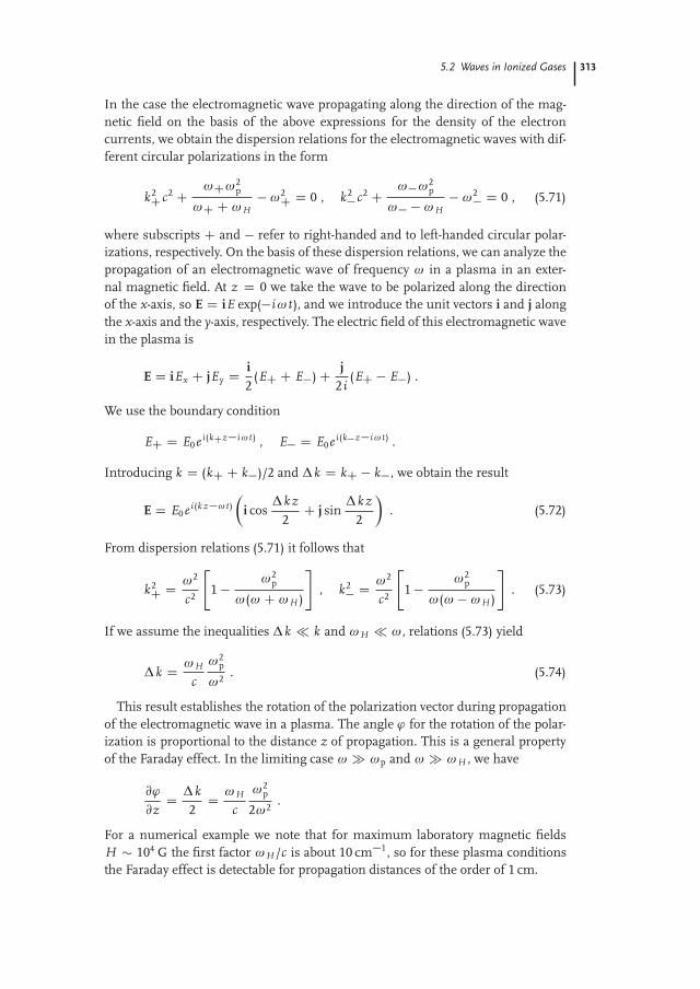
In the case the electromagnetic wave propagating along the direction of the mag-netic field on the basis of the above expressions for the density of the electroncurrents, we obtain the dispersion relations for the electromagnetic waves with dif-ferent circular polarizations in the form
k2Cc2 C ωCω2
p
ωC C ωH� ω2
C D 0 , k2�c2 C ω�ω2
p
ω� � ωH� ω2
� D 0 , (5.71)
where subscripts C and � refer to right-handed and to left-handed circular polar-izations, respectively. On the basis of these dispersion relations, we can analyze thepropagation of an electromagnetic wave of frequency ω in a plasma in an exter-nal magnetic field. At z D 0 we take the wave to be polarized along the directionof the x-axis, so E D iE exp(�i ω t), and we introduce the unit vectors i and j alongthe x-axis and the y-axis, respectively. The electric field of this electromagnetic wavein the plasma is
E D iEx C jEy D i2
(EC C E�) C j2 i
(EC � E�) .
We use the boundary condition
EC D E0e i(kCz�i ω t ) , E� D E0e i(k�z�i ω t ) .
Introducing k D (kC C k�)/2 and Δ k D kC � k�, we obtain the result
E D E0e i(k z�ω t)�
i cosΔ kz
2C j sin
Δ k z2
�. (5.72)
From dispersion relations (5.71) it follows that
k2C D ω2
c2
"1 � ω2
p
ω(ω C ωH )
#, k2
� D ω2
c2
"1 � ω2
p
ω(ω � ωH )
#. (5.73)
If we assume the inequalities Δ k � k and ωH � ω, relations (5.73) yield
Δ k D ωH
c
ω2p
ω2 . (5.74)
This result establishes the rotation of the polarization vector during propagationof the electromagnetic wave in a plasma. The angle ' for the rotation of the polar-ization is proportional to the distance z of propagation. This is a general propertyof the Faraday effect. In the limiting case ω � ωp and ω � ωH , we have
@'
@zD Δ k
2D ωH
c
ω2p
2ω2 .
For a numerical example we note that for maximum laboratory magnetic fieldsH � 104 G the first factor ωH /c is about 10 cm�1, so for these plasma conditionsthe Faraday effect is detectable for propagation distances of the order of 1 cm.

314 5 Waves, Instabilities, and Structures in Excited and Ionized Gases
From the above results it follows that the Faraday effect is strong in the regionof the cyclotron resonance ω � ωH . Then a strong interaction occurs betweenthe plasma and the electromagnetic wave with left-handed polarization. In partic-ular, it is possible for the electromagnetic wave with left-handed polarization to beabsorbed, but for the wave with right-handed circular polarization to pass freelythrough the plasma. Then the Faraday effect can be detected at small distances.
5.2.7
Whistlers
Insertion of a magnetic field into a plasma leads to a large variety of new typesof oscillations in it. We considered above magnetohydrodynamic waves and mag-netic sound, both of which are governed by elastic magnetic properties of a coldplasma. In addition to these phenomena, a magnetic field can produce electronand ion cyclotron waves that correspond to rotation of electrons and ions in themagnetic field. Mixing of these oscillations with plasma oscillations, ion sound,and electromagnetic waves creates many types of hybrid waves in a plasma. As anexample of this, we now consider waves that are a mixture of electron cyclotronand electromagnetic waves. These waves are called whistlers and are observedas atmospheric electromagnetic waves of low frequency (in the frequency inter-val 300–30 000 Hz). These waves are a consequence of lightning in the upper at-mosphere and propagate along magnetic lines of force. They can approach themagnetosphere boundary and then reflect from it. Therefore, whistlers are usedfor exploration of the Earth’s magnetosphere up to distances of 5–10 Earth radii.The whistler frequency is low compared with the electron cyclotron frequencyωH D eH/(me c) � 107 Hz, and it is high compared with the ion cyclotron fre-quency ωiH D eH/(M c) � 102�103 Hz (M is the ion mass). Below we considerwhistlers as electromagnetic waves of frequency ω � ωH that propagate in a plas-ma in the presence of a constant magnetic field.
We employ relation (5.48) to give the oscillatory parameters of a monochromaticelectromagnetic wave. Then (5.68) gives
k2E � k(k � E) � i j4πω
c2 D 0 (5.75)
where ω � kc. We state the current density of electrons in the form j D �eNew,where Ne is the electron number density. The electron drift velocity follows fromthe electron equation of motion (4.157), which, when ν � ω � ωH , has the formeE/me D �ωH (wh), where h is the unit vector directed along the magnetic field.Substituting this into equation (5.75), we obtain the dispersion relation
k2(j h) � k[k � (j h)] � i jωω2
p
ωH c2 D 0 , (5.76)
where ωp D p4πN0e2/me is the plasma frequency in accordance with (1.13).
We introduce a coordinate system such that the z-axis is parallel to the external
5.2 Waves in Ionized Gases 315
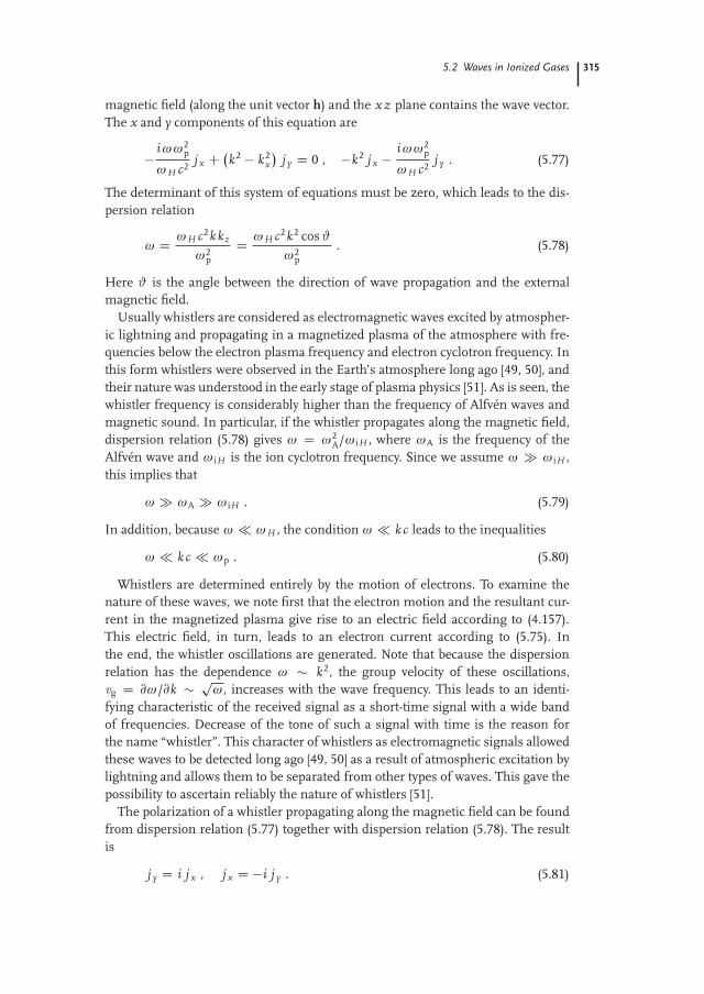
magnetic field (along the unit vector h) and the x z plane contains the wave vector.The x and y components of this equation are
� i ωω2p
ωH c2j x C
k2 � k2x
�j y D 0 , �k2 j x � i ωω2
p
ωH c2j y . (5.77)
The determinant of this system of equations must be zero, which leads to the dis-persion relation
ω D ωH c2kkz
ω2p
D ωH c2k2 cos #
ω2p
. (5.78)
Here # is the angle between the direction of wave propagation and the externalmagnetic field.
Usually whistlers are considered as electromagnetic waves excited by atmospher-ic lightning and propagating in a magnetized plasma of the atmosphere with fre-quencies below the electron plasma frequency and electron cyclotron frequency. Inthis form whistlers were observed in the Earth’s atmosphere long ago [49, 50], andtheir nature was understood in the early stage of plasma physics [51]. As is seen, thewhistler frequency is considerably higher than the frequency of Alfvén waves andmagnetic sound. In particular, if the whistler propagates along the magnetic field,dispersion relation (5.78) gives ω D ω2
A/ωiH , where ωA is the frequency of theAlfvén wave and ωiH is the ion cyclotron frequency. Since we assume ω � ωiH ,this implies that
ω � ωA � ωiH . (5.79)
In addition, because ω � ωH , the condition ω � k c leads to the inequalities
ω � kc � ωp . (5.80)
Whistlers are determined entirely by the motion of electrons. To examine thenature of these waves, we note first that the electron motion and the resultant cur-rent in the magnetized plasma give rise to an electric field according to (4.157).This electric field, in turn, leads to an electron current according to (5.75). Inthe end, the whistler oscillations are generated. Note that because the dispersionrelation has the dependence ω � k2, the group velocity of these oscillations,vg D @ω/@k � p
ω, increases with the wave frequency. This leads to an identi-fying characteristic of the received signal as a short-time signal with a wide bandof frequencies. Decrease of the tone of such a signal with time is the reason forthe name “whistler”. This character of whistlers as electromagnetic signals allowedthese waves to be detected long ago [49, 50] as a result of atmospheric excitation bylightning and allows them to be separated from other types of waves. This gave thepossibility to ascertain reliably the nature of whistlers [51].
The polarization of a whistler propagating along the magnetic field can be foundfrom dispersion relation (5.77) together with dispersion relation (5.78). The resultis
j y D i j x , j x D �i j y . (5.81)

316 5 Waves, Instabilities, and Structures in Excited and Ionized Gases
From this it follows that the wave has circular polarization. This wave propagatingalong the magnetic field therefore has a helical structure. The direction of rotationof wave polarization is the same as the direction of electron rotation. The develop-ment of such a wave can be described as follows. Suppose electrons in a certainregion possess a velocity perpendicular to the magnetic field. This electron motiongives rise to an electric field and compels electrons to circulate in the plane perpen-dicular to the magnetic field. This perturbation is transferred to the neighboringregions with a phase delay. Such a wave is known as a helicon wave.
5.3
Plasma Instabilities
5.3.1
Damping of Plasma Oscillations in Ionized Gases
Interaction of electrons and atoms leads to damping of plasma oscillations becauseelectron–atom collisions shift the phase of the electron vibration and change thecharacter of collective interaction of electrons in plasma oscillations. We shall takethis fact into account below, and include it in the dispersion relation for the plasmaoscillations. To obtain this relation, we use (4.9) instead of (4.6) as the equationfor the average electron momentum. Then the second equation in set (5.56) istransformed into
�i ωw 0 C ik p 0
me N0C eE 0
meD w 0
τ, (5.82)
and the remaining equations of this set are unchanged. Here τ is the characteristictime for elastic electron–atom collisions.
Replacing the first equation in system (5.56) by (5.82), we obtain the dispersionrelation in the form
ω Dq
ω2p C γ
˝v2
x
˛k2 � i
τ(5.83)
instead of (5.57). This dispersion relation requires the condition
ωτ � 1 . (5.84)
Substituting dispersion relation (5.83) into (5.48), we find that the wave ampli-tude decreases with time as exp(�t/τ), where this decrease is due to the scatteringof electrons by atoms of the gas. The condition for existence of plasma oscillationsis such that the characteristic time of the wave damping must be considerably high-er than the oscillation period; namely, inequality (5.84) must hold. The frequency ofcollisions between electrons and atoms is 1/τ � N σv , where N is the atom num-ber density, v is a typical velocity of the electrons, and σ is the cross section forelectron–atom collisions. Assuming this cross section to be of the order of a gas-kinetic cross section, the mean electron energy to be approximately 1 eV, and the
5.3 Plasma Instabilities 317
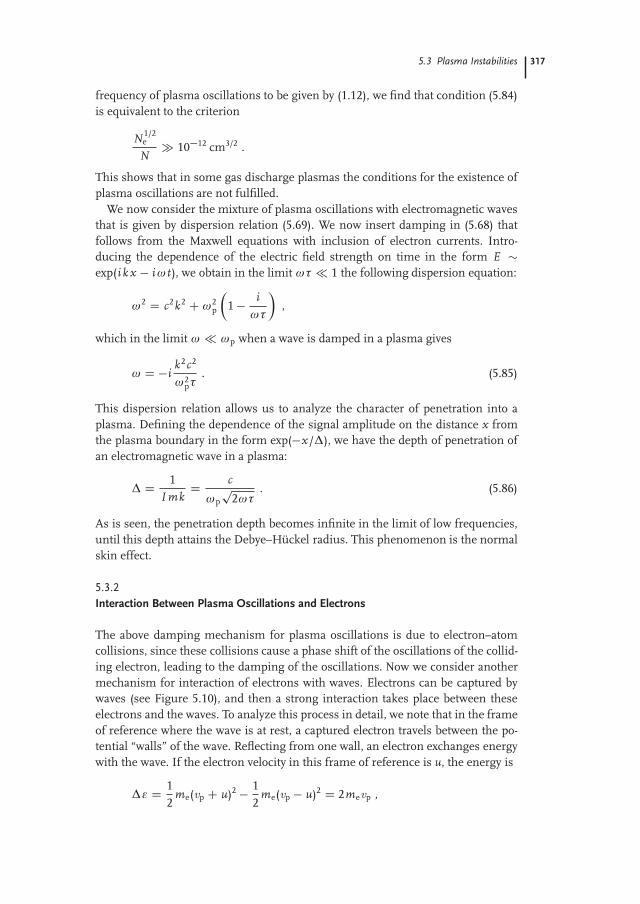
frequency of plasma oscillations to be given by (1.12), we find that condition (5.84)is equivalent to the criterion
N 1/2e
N� 10�12 cm3/2 .
This shows that in some gas discharge plasmas the conditions for the existence ofplasma oscillations are not fulfilled.
We now consider the mixture of plasma oscillations with electromagnetic wavesthat is given by dispersion relation (5.69). We now insert damping in (5.68) thatfollows from the Maxwell equations with inclusion of electron currents. Intro-ducing the dependence of the electric field strength on time in the form E �exp(i kx � i ω t), we obtain in the limit ωτ � 1 the following dispersion equation:
ω2 D c2k2 C ω2p
�1 � i
ωτ
�,
which in the limit ω � ωp when a wave is damped in a plasma gives
ω D �ik2c2
ω2pτ
. (5.85)
This dispersion relation allows us to analyze the character of penetration into aplasma. Defining the dependence of the signal amplitude on the distance x fromthe plasma boundary in the form exp(�x/Δ), we have the depth of penetration ofan electromagnetic wave in a plasma:
Δ D 1I mk
D c
ωpp
2ωτ. (5.86)
As is seen, the penetration depth becomes infinite in the limit of low frequencies,until this depth attains the Debye–Hückel radius. This phenomenon is the normalskin effect.
5.3.2
Interaction Between Plasma Oscillations and Electrons
The above damping mechanism for plasma oscillations is due to electron–atomcollisions, since these collisions cause a phase shift of the oscillations of the collid-ing electron, leading to the damping of the oscillations. Now we consider anothermechanism for interaction of electrons with waves. Electrons can be captured bywaves (see Figure 5.10), and then a strong interaction takes place between theseelectrons and the waves. To analyze this process in detail, we note that in the frameof reference where the wave is at rest, a captured electron travels between the po-tential “walls” of the wave. Reflecting from one wall, an electron exchanges energywith the wave. If the electron velocity in this frame of reference is u, the energy is
Δε D 12
me(vp C u)2 � 12
me(vp � u)2 D 2mevp ,
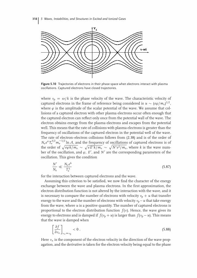
318 5 Waves, Instabilities, and Structures in Excited and Ionized Gases
Figure 5.10 Trajectories of electrons in their phase space when electrons interact with plasma
oscillations. Captured electrons have closed trajectories.
where vp D ω/ k is the phase velocity of the wave. The characteristic velocity ofcaptured electrons in the frame of reference being considered is u � (e'/me)1/2,where ' is the amplitude of the scalar potential of the wave. We assume that col-lisions of a captured electron with other plasma electrons occur often enough thatthe captured electron can reflect only once from the potential wall of the wave. Theelectron obtains energy from the plasma electrons and escapes from the potentialwell. This means that the rate of collisions with plasma electrons is greater than thefrequency of oscillations of the captured electron in the potential well of the wave.The rate of electron–electron collisions follows from (2.38) and is of the order ofNee4T 3/2
e m�1/2e ln Λ, and the frequency of oscillations of captured electrons is of
the order ofp
e'k/me � peE 0k/me � p
N 0e2/me, where k is the wave num-ber of the oscillation, and ', E 0, and N 0 are the corresponding parameters of theoscillation. This gives the condition
N 0
Ne� Ne e6
T 3e
(5.87)
for the interaction between captured electrons and the wave.Assuming this criterion to be satisfied, we now find the character of the energy
exchange between the wave and plasma electrons. In the first approximation, theelectron distribution function is not altered by the interaction with the wave, and itis necessary to compare the number of electrons with velocity vp C u that transferenergy to the wave and the number of electrons with velocity vp � u that take energyfrom the wave, where u is a positive quantity. The number of captured electrons isproportional to the electron distribution function f (v ). Hence, the wave gives itsenergy to electrons and is damped if f (vp C u) is larger than f (vp � u). This meansthat the wave is damped when�
@ f@vx
�vx Dvp
< 0 . (5.88)
Here vx is the component of the electron velocity in the direction of the wave prop-agation, and the derivative is taken for the electron velocity being equal to the phase

5.3 Plasma Instabilities 319
Figure 5.11 The velocity distribution func-
tion for plasma and beam electrons when an
electron beam is injected in a plasma. The
solid curve corresponds to the initial electron
distribution in the plasma and beam. Ranges
with a positive derivation are unstable, and
development of the instability transforms the
distribution function into that indicated by the
dotted line.
velocity vp of the wave. When condition (5.88) is not satisfied, the wave takes energyfrom the electrons and its amplitude increases.
In deriving condition (5.88) for wave damping, we stated that condition (5.87) issatisfied when the field of the wave does not affect the electron distribution func-tion. However, criterion (5.88) holds also when condition (5.87) is not satisfied andthe electron distribution function is altered owing to the interaction with the wave.Interaction with the wave tends to equalize the number densities of electrons withvelocities vp Cu and vp �u and, hence, it decreases the derivative @ f /@vx at vx D vp,albeit without a change in its sign. That is, criterion (5.88) remains valid even whenthe interaction with the wave alters the electron distribution function.
Condition (5.88) is satisfied for the Maxwell electron energy distribution functionor if it is simply a monotonically decreasing function, and oscillations in such aplasma decrease with time owing to the interaction with electrons. However, whenan electron beam is injected into the plasma producing the electron distributionfunction in Figure 5.11, plasma oscillations in this system will be amplified, get-ting the necessary energy from the electrons. The interaction between plasma os-cillations and electrons will reduce the velocity of the electrons until the electrondistribution function again becomes monotonically decreasing.
Amplification of the oscillations can cause their amplitude to increase rapidlywith time. If the oscillation amplitude is small and the oscillations do not alter theelectron distribution function, that is, if condition (5.87) is satisfied, then the oscil-lation amplitude will increase exponentially. When particles of the plasma transfertheir energy to the plasma wave, thus amplifying it, such a plasma state is termedan unstable state.
320 5 Waves, Instabilities, and Structures in Excited and Ionized Gases
5.3.3
Attenuation Factor for Waves in Plasmas
We introduce into relation (5.48) the attenuation factor γ for the waves, so the oscil-lation amplitude varies as exp(�γ t). We can estimate the attenuation factor whenthe wave does not affect the electron distribution in the plasma, so condition (5.87)remains satisfied. Variation with time of the energy density W of the plasma oscil-lations can be estimated to be
d Wdt
� ν
u0Z�u0
f (v )Δεdu . (5.89)
Here ν � u0k is the oscillation frequency for an electron captured in the potentialwell of the wave, u0 D (2e'/me)1/2, ' is the amplitude of the oscillation potential,and Δε D 2mevp u0 is the maximum change in the electron energy when the direc-tion of the electron motion is reversed. (We take into account only the interactionbetween the wave and captured electrons.) The right-hand side of (5.89) may beestimated as
ν@ f@v x
u0Δεu0 � u0k@ f@v x
u0mevpu0 � u0� @ f@v x
e2ωmek 2
W ,
where we use the relations vp D ω/ k and W � (E 0)2 � '2/ k2(E 0 is the amplitudeof the electric field of the wave). From the definition of the attenuation factor γ ofthe plasma wave, we have d W/d t D �γ W , so we obtain the estimate
γ � e2ωmek2
@ f@v x
. (5.90)
Attenuation occurs when condition (5.88) is satisfied. The attenuation factor (5.90),which is due to the interaction between the charged particles and the wave, isknown as the Landau damping factor.
The condition for the existence of oscillations is
γ � ω . (5.91)
We can examine the implications of condition (5.91) for plasma oscillations, andwe can also investigate ion sound, assuming a Maxwell distribution function forthe particles. Taking ω � ωp, we obtain
k rD � 1 (5.92)
for plasma oscillations, where rD is the Debye–Hückel radius (1.7). When this con-dition is fulfilled, the phase velocity of the wave is considerably greater than thethermal velocity, so the electrons captured by the wave are in the tail of the distri-bution function.
When the ion sound propagates in a plasma in which the temperatures of elec-trons and ions are identical, the phase velocity of the ion sound is of the order of
5.3 Plasma Instabilities 321
the thermal velocity of the ions, and the attenuation factor is of the order of thewave frequency. Therefore, ion sound can propagate only in plasmas in which theelectron temperature Te is considerably higher than the ion temperature Ti, that is,when we have
Te � Ti . (5.93)
5.3.4
Beam-Plasma Instability
Assume that an electron beam penetrates into a plasma, where the velocity of theelectrons in the beam is much higher than the thermal velocity of the plasma elec-trons and the number density Nb of the electrons in the beam is considerably lowerthan the number density N0 of plasma electrons. Deceleration of the electron beamcan occur owing to the scattering of electrons of the beam by electrons and ions ofthe plasma. There is, however, another mechanism for deceleration of the electronbeam: beam instability. In the early days of plasma physics this phenomenon wasknown as the Langmuir paradox [26–28]. It was revealed in these investigationsthat when electrons are ejected from a cathode surface in the form of a beam, theaverage energy of ejected electrons becomes equal to the thermal energy of theelectrons of the gas discharge plasma into which this electron beam penetrates, atsmall distances from the cathode as compared with the mean free path of the elec-trons. Because it was assumed in that era that energy exchange between beam andplasma electrons results only from collisions because oscillations of the plasmawere weak, the observed effect was considered to be a paradox. In actuality, interac-tion of the beam electrons with plasma electrons proceeds more effectively throughcollective degrees of freedom of the beam-plasma system than through collisionsdue to the resonant character of this interaction, and this explains the effect un-der consideration [29, 30, 52, 53]. This interaction can be succinctly described asfollows. Suppose plasma oscillations are generated in a plasma. Interacting withelectrons of the beam and taking energy from them, these oscillations are ampli-fied. Thus, some of the energy of the electron beam is transformed into the energyof plasma oscillations and remains in the plasma. This energy may subsequentlybe transferred to other degrees of freedom of the plasma.
One can estimate the amplification of the plasma oscillations in the above sce-nario assuming the oscillation amplitude to be small, and taking the temperaturesof the electrons in the plasma and in the beam to be zero. Hence, the pressure ofthe electrons in the plasma and beam is zero. Applying the continuity equation (4.1)and the Euler equation (4.6) to the plasma electrons, we derive equations for theamplitudes of the plasma parameters that follow from the two first equations ofset (5.91) with p 0 D 0. Elimination of the electron velocity w 0 in the wave in theseequations yields
N 0e D �i
kE 0
meω2N0 . (5.94)
One can obtain the expression for the amplitude of oscillations of the electron num-ber density N 0
b in the beam in a similar way by writing the electron number density

322 5 Waves, Instabilities, and Structures in Excited and Ionized Gases
in the beam as Nb C N 0b exp[i(k x � ω t)] and the velocity of the electrons in the
beam as u C wb exp[i(kx � ω t)], where the x-axis is parallel to the velocity of thebeam and Nb and u are, respectively, the electron number density and the electronvelocity in the unperturbed beam. Then we have
N 0b D � i kE 0Nb
me(ω � ku)2 . (5.95)
As was done in arriving at the last equation of system (5.56), the Poisson equa-tion (3.2) yields
i kE 0 D �4πe(N 0e C N 0
b) (5.96)
for the amplitude of the system’s parameters. Eliminating the amplitudes N 0, N 0b,
and E 0 from the set of equations (5.94), (5.95), and (5.96), we obtain the dispersionrelation
ω2p
ω2 C ω2p
(ω � ku)2 � Nb
N0D 1 . (5.97)
Here ωp D (4πN0e2/me)1/2 is the frequency of plasma oscillations in accordancewith (1.12). When the number density of the beam electrons is zero (Nb D 0),dispersion relation (5.97) reduces to (5.57), where the electron temperature is takento be zero. The strongest interaction between the beam and plasma occurs whenthe phase velocity of the plasma waves ω/ k is equal to the velocity of the electronbeam. Let us analyze this case. Since the number density of the beam electronsNb is small compared with the number density N0 of the plasma electrons, thefrequency of the plasma oscillations is close to the plasma frequency ωp. Hence,we shall consider waves with wave number k D ω/u, which have the most effectiveinteraction with the electron beam. We write the frequency of these oscillations asω D ωp C δ and insert it into dispersion relation (5.97). Expanding the result in aseries in terms of the small parameter δ/ωp, we obtain
δ D ωp
�Nb
2N0
�1/3
exp�
2π i n3
�,
where n is an integer. One can see that δ/ωp � (Nb/N0)1/3 � 1. That is, theexpansion over the small parameter δ/ωp is valid.
If the imaginary component of the frequency (which is equal to the imaginarycomponent of δ) is negative, the wave is attenuated; if it is positive, the wave isamplified. The maximum value of the amplification factor is given by (n D 1)
�γ Dp
32
�Nb
N0
�1/3
ωp D 0.69ωp
�Nb
N0
�1/3
. (5.98)
The amplitude N 0b varies with time as exp(γ t); this result is valid if the plasma
oscillations do not affect the properties of the plasma. This type of instability isknown as beam-plasma instability. As a result of this instability, the distributionfunction for the beam electrons expands (see Figure 5.11), and the energy surplus istransferred to plasma oscillations. In reality, various factors influence the characterand rate of a beam of charged particles propagating in a plasma [54].
5.3 Plasma Instabilities 323
5.3.5
Buneman Instability
We now consider instability of another type that develops if the mean velocity ofthe electrons differs from the mean velocity of the ions. We formulate the prob-lem by taking all the plasma ions to be at rest and all the electrons to be travelingwith velocity u with respect to the ions. The plasma is quasineutral, that is, thenumber densities of the electrons and ions are equal. Our goal is to determinethe maximum amplification factor of the plasma oscillations. The electron beam isdecelerated owing to the transfer of energy from the beam to the plasma oscilla-tions [55].
With this formulation, the problem is equivalent to the previous case of inter-action of an electron beam and a plasma. In both problems an electron beam ispenetrating a plasma, so the dispersion relation can be derived in a similar way.Denoting the ion mass as M and taking into account the equality of ion and elec-tron number densities, we obtain the dispersion relation
me
M
ω2p
ω2 C ω2p
(ω � ku)2 D 1 (5.99)
instead of (5.97). If we let the ratio me/M go to zero, we obtain the dispersion rela-tion ω D ωp C ku. Hence, one can write the frequency of the plasma oscillationsas
ω D ωp C ku C δ .
Substituting this frequency into dispersion relation (5.99) and expanding the resultin a power series in terms of the small parameter δ/ωp, we obtain
2δωp
D me
M
ω2p
(ωp C ku C δ)2 .
The electron beam has the strongest interaction with the wave whose wave numberis k D �ωp/u. For this wave we have
δ D�me
M
�1/3ωp exp
�2π i n
3
�,
where n is an integer. The highest amplification factor corresponds to n D 1 and isgiven by
�γ D I mδ Dp
32
� me
2M
�1/3ωp D 0.69ωp
�me
M
�1/3. (5.100)
Note that the frequency of oscillations is the order of the amplification factor. Thistype of instability of the electron beam due to interaction with plasma ions is knownas Buneman instability [55]. This instability can exist in an ionospheric plasma [56]and in a hot or nonequilibrium plasma [57].

324 5 Waves, Instabilities, and Structures in Excited and Ionized Gases
5.3.6
Hydrodynamic Instabilities
The instabilities discussed above are so-called kinetic instabilities, for which theamplification of oscillations is due to the differences in the character of the motionof various groups of particles [59, 60]. The development of oscillations ultimatelyresults in a change of the velocity distribution function for the charged particlesof the plasma. Another class of instabilities is known as hydrodynamic instabil-ities. The development of hydrodynamic instabilities involves a displacement ofthe plasma regions and results, finally, in variation of the spatial configuration ofthe plasma. We shall analyze the simplest type of hydrodynamic instability, pinchinstability.
We examine the stability of the pinch configuration with respect to variation ofa current radius at a given point where the current axial symmetry is conservedat such a variation. The corresponding instability is called a sausage instability.We have to find under what conditions an accidental distortion of the pinch willnot develop further. Let us assume that the distortion of the pinch results onlyin a slight curving of the magnetic lines of force; that is, the radius of curvatureof the magnetic lines of force is considerably larger than the radius of the pinch.According to (4.163), the relation [58]
p C H2
8πD const
is satisfied in the plasma region.We must analyze the variation of the parameters of the pinch due to variation
of its radius. The total current and magnetic flux through the cross section of thepinch will be conserved. The electric current is Iz D caH'/2, where a is the pinchradius and H' is the axial magnetic field strength. The condition δ Iz D 0 yields(δa/a) C (δH'/H' ) D 0, where δa is the variation of the pinch radius, and δH' isthe variation of the axial magnetic field at the pinch surface outside the plasma. Thelongitudinal magnetic field is frozen into the plasma, so a displacement of plasmaelements does not change the magnetic flux through them. The condition for con-servation of the magnetic flux, Φz D πa2Hz , yields (2δa/a) C (δHz/Hz ) D 0,where Hz is the longitudinal external magnetic field as it exists inside the plasma.Hence, (δHz/Hz D 2(δH'/H' ). The variation of the magnetic field pressure in-side the plasma is δ[H2
z /(8π)] D Hz δHz/(4π), and the variation of the magneticpressure outside the plasma is H' δH'/(4π) D H2
' δHz/(8πHz ). It can be seenthat if
H2z � H2
'
2(5.101)
holds true, the additional internal magnetic field pressure produced by the distor-tion of the pinch is smaller than the additional external magnetic field pressure.When condition (5.101) is satisfied, the pinch is stable with respect to displace-ments of the sausage type.

5.4 Nonlinear Phenomena in Plasmas 325
5.4
Nonlinear Phenomena in Plasmas
5.4.1
The Lighthill Criterion
Plasma instabilities cause the development of certain types of oscillations. The sub-sequent evolution of these oscillations is determined by interactions between theoscillations and the plasma itself. The strength of these interactions depends onthe wave amplitude. Hence, if a plasma instability develops, we deal with nonlin-ear plasma phenomena. But the role of nonlinear plasma processes is not restrict-ed to the development of instabilities [61]. Nonlinear processes affect the natureof wave propagation in a plasma. In fact, interaction between elementary wavesacts through the interaction of these waves with the plasma. Therefore, nonlinearphenomena determine both the profile and the character of the propagation of allwaves in a plasma except those of low intensity. Along with this, nonlinear phe-nomena create a new plasma state [54, 62–64].
To study the development of perturbations in a plasma, we examine a perturba-tion in the form of a one-dimensional wave packet consisting of waves encompass-ing a narrow range of wave numbers (Δ k � k). The perturbation amplitude atpoint x is
a(x , t) DX
k
a(k) exp(i kx � i ω t) , (5.102)
where a(k) is the amplitude of the wave with wave number k. We take into accountthe wave dispersion, expressible as [65]
ω(k) D ω(k0) C @ω(k0)@k
(k � k0) C @2ω(k0)@k2 (k � k0)2
D ω0 C vg(k � k0) C 12
@vg(k0)@k
(k � k0)2 . (5.103)
Here k0 is the mean wave number of the wave packet and vg is the group velocity ofthe wave. Since wave number values are restricted to an interval of width Δ k neark0, then according to (5.102) the perturbation is initially concentrated in a spatialregion of extent Δx � 1/Δ k. As the wave packet evolves, it diverges owing to thedifferent group velocities of individual waves. The initial wave packet, which has asize of the order of 1/Δ k, diverges on a timescale given by τ � (Δ k2)�1(@vg/@k)�1.That is, the wave dispersion usually leads to increasing spatial extension of the waveas a function of time.
The interaction of waves of different k values influences the behavior of thisprocess. In particular, it can even lead to compression of the waves. To assess thispossibility, we take into account the dependence
ω D ω0 � αE 2 (5.104)

326 5 Waves, Instabilities, and Structures in Excited and Ionized Gases
of the wave frequency on its amplitude, where E is a (small) field amplitude and ω0
is the frequency of this wave. Inserting expansions (5.103) and (5.104) into (5.102),we obtain
a(x , t) DX
k
a(k)
exp�
i(k � k0)(x � x0) � i k0x0 � i(k � k0)2 @vg
@kt � i αE 2(x )t
�(5.105)
for the wave packet amplitude. From (5.105) it follows that nonlinear wave interac-tions can lead to modulation of the wave packet. With certain types of modulationthe wave packet may decay into separate bunches, or it may be compressed into asolitary wave – a soliton. This phenomenon is known as modulation instability.
Formula (5.105) shows that the compression of a wave packet or its transforma-tion into separate bunches can take place only if the last two terms in the exponentin this equation have opposite signs. Only in this case can a nonlinear interactioncompensate for the usual divergence of the wave packet. Therefore, the modulationinstability can only occur if the following criterion holds true:
α@vg
@k< 0 . (5.106)
This condition is called the Lighthill criterion [66].
5.4.2
The Korteweg–de Vries Equation
The above analysis shows that wave dispersion leads to divergence of the wavepacket. If this divergence is weak, a weak nonlinearity is able to change its character.We now consider an example of such behavior when a wave is characterized by lowdispersion and nonlinearity. Consider the propagation of long-wavelength waves ina medium in which the dispersion relation has the form
ω D vg k(1 � r20 k2) , r0k � 1 . (5.107)
This form describes a variety of oscillations, with sound and ion sound as examples.We shall obtain below a nonlinear equation that describes such waves.
We take as the starting point the Euler equation (4.6) for the velocity of particlesin a longitudinal wave that has the form
@v@t
C v@v@x
� Fm
D 0 . (5.108)
Here v (x , t) is the particle (gas atom or gas molecule) velocity in a longitudinalwave which propagates along the x-axis, F is the force per atomic particle, and m isthe mass of the atomic particle. Within the framework of a linear approximation,

5.4 Nonlinear Phenomena in Plasmas 327
one can write the particle velocity in the form v D vg C v 0, where vg is the groupvelocity and v 0 is the particle velocity in the frame of reference where the wave is atrest. Because v 0 � vg, we have
@v 0
@tC vg
@v 0
@x� F
mD 0
in the linear approximation, where the last term is a linear operator with respectto v 0. In the harmonic approximation we have v 0 � exp(i k x � i ω t). We seek theform of the operator F/m that leads to dispersion relation (5.107) in this approach.This gives
@v@t
0
C vg
�@v 0
@xC r2
0@3v 0
@x3
�D 0 .
The last term takes into consideration a weak dispersion of long-wave oscillations.To account for nonlinearity of these waves, we analyze the second term of thisequation. In the linear approach we replace the particle velocity v by the groupvelocity vg. Returning this term to its initial form, that is, taking into account weaknonlinear effects, we obtain
@v@t
C v@v@x
C vg r20
@3v@x3
D 0 . (5.109)
This equation is called the Korteweg–de Vries equation [67] and was originally ob-tained in the analysis of wave propagation processes in shallow water.
The Korteweg–de Vries equation accounts for nonlinearity and weak dispersionsimultaneously, and therefore serves as a convenient model equation for the anal-ysis of nonlinear dissipative processes. As applied to plasmas, it describes propa-gation of long-wavelength waves in a plasma for which the dispersion relation isgiven by (5.107).
5.4.3
Solitons
The Korteweg–de Vries equation has solutions that describe a class of solitarywaves. These waves are called solitons and conserve their form in time. It fol-lows from dispersion relation (5.107) that short waves propagate more slowly thanlong waves, but nonlinear effects compensate for the spreading of the wave. Wenow show that this property holds true for waves that are described by the Ko-rteweg–de Vries equation. We consider a wave of velocity u. The spatial and tem-poral dependence for the particle velocity has the form v D f (x � ut). This gives@v/@t D �u@v/@x , and the Korteweg–de Vries equation is transformed to the form
(v � u)dvdx
C vg r20
d3vdx3
D 0 . (5.110)

328 5 Waves, Instabilities, and Structures in Excited and Ionized Gases
Assuming the perturbation to be zero at large distances from the wave, that is v D 0and d2v/dx2 D 0 at x ! 1, this equation reduces to
vg r20
d2vdx2 D uv � v2
2,
with the solution
v D 3u cosh�2
x
2r0
suvg
!. (5.111)
The wave described by (5.111) is concentrated in a limited spatial region and doesnot diverge in time. The wave becomes narrower with an increase of its ampli-tude, that is, the wave is concentrated in a restricted region, and its spatial width isinversely proportional to the square root of the wave amplitude.
In other words, the Korteweg–de Vries equation has stationary solutions describ-ing a nonspreading solitary wave, or soliton. The amplitude a and extension 1/αof solitons are such that the value a/α2 does not depend on the wave amplitude.If the initial perturbation is relatively small, evolution of the wave packet leads toformation of one solitary wave. If the amplitude of an initial perturbation is rela-tively large, this perturbation in the course of evolution of the system will split intoseveral solitons. Thus, solitons are not only stable steady-state perturbations in thesystem, but they can also play a role in the evolution of some perturbations in anonlinear dispersive medium.
5.4.4
Langmuir Solitons
The occurrence and propagation of solitons is associated with an electric field thatexists in a plasma as the result of a wave process, and this field confines the per-turbation to a restricted region. This can be demonstrated using the example ofplasma oscillations. Denoting by E(x , t) the electric field strength of the plasmaoscillations, we have
W(x ) D E 2
8π
for their energy density, where the bar means a time average. Assuming the equal-ity of electron and ion temperatures, Te D Ti D T , the pressure of a quasineutralplasma is p D 2Ne T . The plasma pressure is established with a sound velocity thatis greater than the velocity of propagation of long-wave oscillations. Then, becauseof the uniformity of plasma pressure at all points of the plasma, we have
2N(x )T C W(x ) D 2N0T , (5.112)
where N0 is the number density of charged particles at large distances where theplasma oscillations are absent, and the plasma temperature is assumed to be con-stant in space.

5.4 Nonlinear Phenomena in Plasmas 329
The dispersion relation for plasma oscillations (5.57) has the form
ω2 D ω2p
1 � E 2
16πN0T
!C γ
˝v2
x
˛k2 (5.113)
when (5.112) is taken into account, where ωp is the plasma frequency in the ab-sence of fields. In (5.113) we used (1.12) for the plasma frequency.
We can write (5.113) in a more convenient form. Take the electric field strengthof the wave in the form E D E0 cos ω t, so E 2 D E 2
0 /2. Using v2x D T/me for
electrons and introducing the Debye–Hückel radius rD according to (1.7), we rep-resent (5.113) in the form
ω2 D ω2p
�1 � E 2
0
32πN0TC 2γ r2
D k2�
. (5.114)
The first term on the right-hand side of this expression is considerably larger thanthe other two terms.
One can see that dispersion relation (5.114) satisfies the Lighthill criterion (5.106)because in this case we have
α@vg
@kD � γ ωp
32πme N0< 0 .
Thus, nonlinear Langmuir oscillations can form a soliton. Dispersion relation(5.114) shows that if the energy density of plasma oscillations is high enough(so that the second term of (5.114) is larger than the third one), the oscillationscannot exist far from the soliton. The oscillations create a potential well in theplasma and are enclosed in this well. They can propagate in the plasma togetherwith the well and occupy a restricted spatial region. The size of the potential well(or the soliton size) decreases with increase of the energy density of the plasmaoscillations. Because rD k � 1, the solitons are formed when the energy densityof the oscillations is small compared with the specific thermal energy of chargedparticles of the plasma. Thus, this analysis demonstrates the tendency to formsolitons from long-wave plasma oscillations. However, the analysis used does notallow one to study the evolution of oscillations at large amplitudes. Nevertheless,this exhibits the conditions for the existence of the Langmuir soliton that wererealized experimentally [68–72] and that can exist in a solar plasma [73].
5.4.5
Nonlinear Ion Sound
We now analyze nonlinear ion sound when the nonlinearity is large [74]. For thispurpose we use the Euler equation (4.6), the continuity equation (4.1), and the Pois-son equation (1.4), which, in the linear approach, leads to dispersion relation (5.62)for ion sound. When we use these equations without any linear approximation,they can be written as
@vi
@tC vi
@vi
@xC e
mi
@'
@xD 0 ,
@Ni
@tC @(Nivi)
@xD 0 ,
@2'
@x2D 4πe(Ne � Ni) . (5.115)

330 5 Waves, Instabilities, and Structures in Excited and Ionized Gases
Here mi is the ion mass, vi is the velocity of ions in the wave, ' is the electric po-tential of the wave, and Ne and Ni are the number densities of electrons and ions,respectively. As discussed above, electrons are in equilibrium with the field owingto their high mobility. Therefore, the Boltzmann distribution applies to the elec-trons, so Ne D N0 exp(e'/Te), where N0 is the mean number density of chargedparticles and Te is the electron temperature.
We now analyze the motion of ions in the field of a steady-state wave when theplasma parameters vi, Ni, and ' depend on time and the spatial coordinate as f (x�ut), where u is the velocity of the wave. Then the set of equations (5.115) can berewritten as
(vi � u)dvi
dxC e
mi� d'
dxD 0 ,
ddx
[Ni(vi � u)] D 0 ,
d2'
dx2 D 4πe�
N0 exp�
e'
Te
�� Ni
�. (5.116)
The perturbation is assumed to be zero far from the wave, so Ni D N0, vi D 0 and' D 0 at x ! 1. The first two equations of set (5.116) then give
v2i
2� uvi C e'
miD 0 , Ni D N0
uu � vi
.
The second equation implies that vi < u because Ni > 0. This means that ' �0 in the first equation, that is, the electric potential of this ion acoustic wave, isalways positive. The first equation leads to vi D u�pu2 � 2e'/mi, and the secondequation gives Ni D N0u(u2�2e'/mi)�1/2. Substituting these expressions into thelast equation of system (5.116), we obtain
d2'
dx2 D 4πeN0
"exp
�e'
Te
�� up
u2 � 2e'/mi
#(5.117)
for the ion sound. This equation describes the potential of the electric field for thenonlinear ion acoustic wave. It is in the form of an equation of motion for a particleif ' is regarded as the coordinate and x as time. A general property of this type ofequation is that multiplication by the integration factor d'/dx makes it possible toperform one integration immediately. Equation (5.117) then becomes
12
�d'
dx
�2
� 4πN0Te exp�
e'
Te
�� 4πN0miu
su2 � 2e'
miD const .
Assuming that at large distances from the wave the potential ' and the electricfield strength of the wave �d'/dx are zero, we can evaluate the constant of inte-
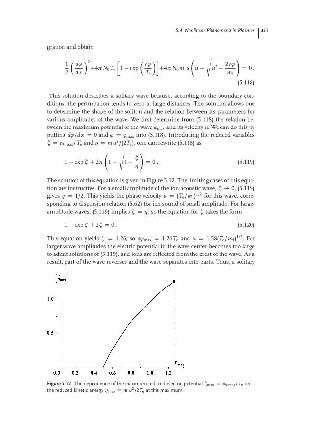
5.4 Nonlinear Phenomena in Plasmas 331
gration and obtain
12
�d'
dx
�2
C4πN0Te
�1 � exp
�e'
Te
��C4πN0miu
u �
su2 � 2e'
mi
!D 0 .
(5.118)
This solution describes a solitary wave because, according to the boundary con-ditions, the perturbation tends to zero at large distances. The solution allows oneto determine the shape of the soliton and the relation between its parameters forvarious amplitudes of the wave. We first determine from (5.118) the relation be-tween the maximum potential of the wave 'max and its velocity u. We can do this byputting d'/dx D 0 and ' D 'max into (5.118). Introducing the reduced variables� D e'max/Te and η D mu2/(2Te), one can rewrite (5.118) as
1 � exp � C 2η
1 �
s1 � �
η
!D 0 . (5.119)
The solution of this equation is given in Figure 5.12. The limiting cases of this equa-tion are instructive. For a small amplitude of the ion acoustic wave, � ! 0, (5.119)gives η D 1/2. This yields the phase velocity u D (Te/mi)1/2 for this wave, corre-sponding to dispersion relation (5.62) for ion sound of small amplitude. For large-amplitude waves, (5.119) implies � D η, so the equation for � takes the form
1 � exp � C 2� D 0 . (5.120)
This equation yields � D 1.26, so e'max D 1.26Te and u D 1.58(Te/mi)1/2. Forlarger wave amplitudes the electric potential in the wave center becomes too largeto admit solutions of (5.119), and ions are reflected from the crest of the wave. As aresult, part of the wave reverses and the wave separates into parts. Thus, a solitary
Figure 5.12 The dependence of the maximum reduced electric potential �max D e'max/Te on
the reduced kinetic energy ηmax D mi u2/2Te at this maximum.

332 5 Waves, Instabilities, and Structures in Excited and Ionized Gases
ion acoustic wave exists only in a restricted range of wave amplitudes and velocities.Exceeding the limiting amplitude leads to a wave decaying into separate waves.
5.4.6
Parametric Instability
Nonlinear phenomena are responsible for interaction between different modes ofoscillation. A possible consequence of this interaction is the decay of a wave intotwo waves. Since the wave amplitude depends on time and spatial coordinates bythe harmonic dependency exp(i k � r � i ω t), such a decay corresponds to fulfillingthe relations
ω0 D ω1 C ω2 , k0 D k1 C k2 , (5.121)
where subscript 0 relates to the parameters of the initial wave and subscripts 1and 2 refer to the decay waves. This instability is called parametric instability. Weconsider below an example of this instability in which a plasma oscillation decaysinto a plasma oscillation of a lower frequency and an ion acoustic wave (ion sound).
The electric field of the initial plasma oscillation is
E D E0 cos(k0x � ω0 t) ,
where x is the direction of propagation. In the zero approximation we assumethe electric field amplitude E0 and other wave parameters to be real values. Theequation of motion for electrons me dv0/d t D �eE yields the electron velocityv0 D u0 cos(k0x � ω0 t), where u0 D eE0/(me ω0).
Let another plasma wave and the ion sound wave be excited in the system si-multaneously with the initial plasma oscillation, and let their amplitudes be smallcompared with the amplitude of the initial oscillation. Consider the temporal de-velopment of these waves taking into account their interaction with each other andwith the initial oscillation. Since ion velocities are much lower than electron ve-locities, one can analyze these waves separately. The equation of motion and thecontinuity equation for ions are
midvi
d tD eE ,
@N 0i
@tC N0
@vi
@xD 0 .
Here mi is the ion mass, vi is the ion velocity, N0 is the equilibrium number densityof ions, N 0
i is the perturbation of the ion number density due to the oscillation,and E is the electric field due to the oscillations. Elimination of the ion velocityfrom these equations yields
@2N 0i
@t2 C eN0
mi
@E@x
D 0 . (5.122)
One can find the electric field strength from the equation of motion for the elec-trons by averaging over fast oscillations. The one-dimensional Euler equation (4.6)

5.4 Nonlinear Phenomena in Plasmas 333
can be rewritten for electrons as
@ve
@tC ve
@ve
@xC 1
me N@pe
@xC eE
meD 0 , (5.123)
where pe D N Te is the the electron gas pressure, Te is the electron temperature,and Ne is the electron number density. After averaging over fast oscillations, wefind the first term in this equation is zero. We write the electron velocity as ve Dv0 C v 0
e, where v 0e is the electron velocity due to the small-amplitude plasma wave.
Then we have
ve@ve
@xD 1
2@v2
e
@xD 1
2@
@x(v0 C v 0
e)2 D @
@x(v0v 0
e) ,
where the bar denotes averaging over fast oscillations. We assume that Te D const,corresponding to a high rate of energy exchange in the ion acoustic wave. Duringthe ion motion, the electron number density has a relaxation time for maintainingthe quasineutrality of the plasma. Therefore, after averaging, we find the deviationof the electron number density from equilibrium is the same as that for ions, andthe third term in the Euler equation (4.6) becomes
1meN
@pe
@xD Te
me N0
@N 0i
@x(N � N0) .
The Euler equation after averaging is transformed into
@
@x
v0v 0
e
�C Te
meN0
@N 0i
@xC eE
meD 0 .
Substituting the electric field derived from this equation into (5.122), we obtain
@2N 0i
@t2 � Te
mi
@2N 0i
@x2 � me N0
mi
@2
@x2
v0v 0
e
� D 0 . (5.124)
If we ignore the last term in (5.124) and assume harmonic dependence of theion density on time and spatial coordinates, we obtain dispersion relation (5.62) forion sound: ω D csk, cs D p
T/mi. To take into account interaction between ionsound and plasma oscillations, we have to trace the motion of electrons in the fieldof the small-amplitude plasma wave. To do this, we shall use the Maxwell equationfor the electric field of the small-amplitude wave, assuming the magnetic field tobe zero. This gives @E 0/@t C 4π j 0 D 0. Here E 0 is the electric field of the wave andj 0 is the electric current density generated by it.
For simplicity, we shall ignore thermal motion of the electrons, since it has onlya small effect on the oscillation frequency. Therefore, when writing the expressionfor the current density, we can ignore the variation of the electron number densitydue to the electron pressure of the plasma wave. We assume the electron numberdensity to have the form Ne C N 0
i , where Ne includes the equilibrium electronnumber density and its variation under the action of the initial plasma wave and N 0
iis the variation of the ion number density owing to the motion of ions. Accordingly,

334 5 Waves, Instabilities, and Structures in Excited and Ionized Gases
the electron velocity is v0 C v 0e, where v0 is the electron velocity due to the initial
plasma wave and v 0e is the electron velocity due to the small-amplitude plasma wave.
The current density due to the small-amplitude plasma wave is then
j 0 D �e(Ne C N 0i )(v0 C v 0
e) C eNev0 D �eNev 0e � eN 0
i v0 ,
where we ignore second-order terms. The Maxwell equation @E 0/@t C 4π j 0 D 0can now be rewritten as
@E 0
@t� 4πeN 0
i v0 � 4πeNev 0e D 0 .
The electron equation of motion is
medv 0
e
d tD �eE 0 .
Eliminating E 0 from these equations, we obtain
@2v 0e
@t2C ω2
pv0e C N 0
i
Neω2
pv0 D 0 (5.125)
as the equation for the electron velocity due to the small-amplitude plasma wave.Here ωp D p
4πNee2/me is the frequency of plasma oscillations ignoring thethermal motion of electrons. One can see that if we do not take into account theinteraction between the small-amplitude plasma wave and the initial plasma os-cillation and the ion acoustic wave (that is, if we ignore the last term in (5.125)),then the assumptions used here give the small-amplitude plasma wave frequencyas being equal to the plasma frequency.
Let us represent the solutions of (5.124) and (5.125) in the form
v0 D u0 cos(k0x � ω0 t) , ve D a cos(kex � ωe t) , N 0i D bN0 cos(kix � ωi t) ,
where a and b are slowly varying oscillation amplitudes, ωe and ke are the frequen-cy and the wave number of the small-amplitude plasma wave, ωi and ki are thefrequency and the wave number of the ion sound, and N0 is the equilibrium num-ber density of the charged particles. (We assume that Ne D N0 in (5.125).) Sincethe oscillation amplitudes vary slowly, the temporal and spatial dependencies areidentical, so we find from (5.124) and (5.125) that
ω0 D ωe C ωi I k0 D ke C ki , (5.126)
as in (5.121). This condition is similar to that for parametric resonance of coupledoscillators, and therefore the instability that we analyze is termed a parametric in-stability. In addition, because of the nature of this process, this instability is calledmodulation instability. This instability has a universal character and is suitable bothfor plasma oscillations and for electromagnetic waves [75, 76].
Taking into account a slow variation of the oscillation amplitudes and condi-tion (5.126), we find from (5.124) and (5.125) [35]
@a@t
D bωe u0
4,
@b@t
D �ameki u0
4miωi
5.5 Ionization Instabilities and Plasma Structures 335
for the oscillation amplitudes. Solution of these equations shows that the oscilla-tions increase with the dependence a, b � exp(γ t), with
γ D 14
rme ωe
miωiu0ki D 1
4
rmeωe
miωi� eE0
meω0ki . (5.127)
Thus, the initial plasma wave is unstable. It can decay into a plasma wave of a lowerfrequency and the ion sound. This instability is also known as decay instability. Theexponential growth parameter of the new wave is proportional to the amplitude ofthe decaying wave.
5.5
Ionization Instabilities and Plasma Structures
5.5.1
Drift Waves
A laboratory ionized gas is usually maintained by an external electric field thatgenerates an electric current and causes ionization of the gas. Electrons are theprincipal plasma component in the sense that electrons contribute most of thetotal electric current, and formation of new charged particles is due to collisionsof electrons with gas atoms or molecules. Perturbations of the electron numberdensity are thus of central importance to the properties of the plasma.
To examine the simplest form of perturbations in the plasma, we begin with thecontinuity equation (4.1)
@Ne
@tC div j D 0
for electrons, and we assume that the electron flux j is determined solely by theelectron drift in an external electric field. The current is then j D wNe, where w isthe electron drift velocity. Using expansion (5.48) for a perturbation to the electronnumber density, we obtain the dispersion relation
ω D kw . (5.128)
That is, there is a wave associated with the perturbation that propagates togetherwith the electric current. In other words, the perturbation moves together withthe electric current. Such waves which transfer plasma perturbation by an electriccurrent are drift waves.
Damping or amplification of these waves can occur by several mechanisms. Onesuch mechanism is the diffusive motion of the electrons. The electron flux is thenj D wNe � Dr Ne, where D is the diffusion coefficient for electrons in a gas, andthe dispersion relation that follows from the continuity equation for electrons hasthe form
ω D kw � i D k2 . (5.129)

336 5 Waves, Instabilities, and Structures in Excited and Ionized Gases
The diffusion of the electrons is seen to lead to damping of the drift wave becausethe dependence of electron parameters on time has the form exp(�i ω t). As a resultof electron diffusion, the perturbation region increases in size and the perturbationdissipates.
The behavior of the drift wave depends on the type of ionization processes in thegas. Under certain conditions, the interaction of drift waves with the ionization pro-cess of gas atoms by electron impact leads to amplification of the drift waves. Thisphenomenon is called ionization instability. Various types of ionization instabilitycan occur depending on the particular properties of a plasma and the processeswithin it. The development of ionization instability leads to the formation of struc-tures in the plasma that will be considered below.
5.5.2
Ionization Instability from Thermal Effects
A common causal mechanism for ionization instability is to be found in the pos-itive column of an arc, where the instability arises from thermal processes. Theequilibrium electron number density depends strongly on the plasma temperature,whereas the temperature dependence of the heat transport coefficient is weak. Athigh intensities, thermal instability occurs because the heat transport mechanismdue to atom thermal conductivity is unable to provide heat release. This instabilitymay lead to contraction of the plasma that increases heat release or it can cause theformation of new types of structures in the plasma. A simple example of this phe-nomenon arises when the heat transport in a cylindrical discharge tube dependsupon thermal conductivity. The heat balance equation in this case has the form
1�
dd�
���(�)
dTd�
�C p (�) D 0 , (5.130)
where � is the distance from the tube axis, � is the thermal conductivity coefficient,and p (�) D i E is the specific power of heat release, where i is the current den-sity and E is the electric field strength. We assume that the rate of heat release isstrongly dependent on the local plasma temperature, and is a function only of thistemperature.
This model is descriptive of arc discharges at high currents and high pressures.If the gas discharge plasma is in equilibrium, the electron and gas temperaturesare similar, and the electron number density can be estimated from the Saha for-mula (1.52) to behave as Ne � exp[� J/(2T )], where J is the ionization potential ofthe gas atoms, and it is usually true that T � J . The specific power of heat releaseis p D i E , where the electric field strength E does not vary over the discharge crosssection, and the variation of the current density i is proportional to Ne. The specificpower of heat release in an arc discharge is determined not only entirely by thetemperature, but also has a strong dependence on the temperature. In this case theequilibrium between ionization and recombination is maintained at each point inthe plasma, that is, local ionization equilibrium is supported in the plasma.

5.5 Ionization Instabilities and Plasma Structures 337
We introduce the new variables z D �2/r20 and θ D (T � Tw)/Tw into (5.130),
where r0 is the tube radius and Tw is the wall temperature. Then (5.130) can bewritten in the form
ddz
�z
dθdz
�C A exp(bθ ) D 0 , (5.131)
where A D r20 p (Tw)/[4Tw�(Tw)], b D Twd ln p (Tw)/dTw, and in this case
b � 1. Because of the strong dependence of p on T, we can assume that thethermal conductivity coefficient � is independent of the temperature. The solutionof (5.131) is given by the Fock formula:
θ D 1b
ln2γ
Ab(1 C γ z)2, (5.132)
where γ is a parameter to be determined by boundary conditions. One of theboundary conditions of (5.131) is θ (0) D 0, following from the definition of thisfunction. This gives the relation for γ that
2γ D Ab(1 C γ )2 . (5.133)
Since γ is real, we have Ab 1/2. If this condition is not satisfied, then (5.131) hasno real solution. This means that thermal instability arises because heat extractionis not compensated for by heat release. The instability then leads to a differentdischarge regime where the current occurs in a narrow region near the tube center.
The threshold for this instability corresponds to γ D 1 and Ab D 1/2, that is, ithas its onset when p (T0) D 4p (Tw), where T0 is the temperature at the axis. Theinstability threshold at Ab D 1/2 corresponds to�
d p (T )dT
�Tw
D 2�(Tw)r2
0. (5.134)
If this instability leads to contraction of the plasma, these relations make it possi-ble to estimate the radius �0 for the new contracted regime of the plasma. Formu-la (5.134) then gives
�20 � �(T0)
�d p (T )
dT
��1
TDT0
, (5.135)
where T0 is the temperature at the axis.
5.5.3
Ionization Wave in a Photoresonant Plasma
In considering a photoresonant plasma in Section 3.3.9, we found two regimesof plasma to exist. In the regime of low intensities of incident resonant radiationbeing absorbed in a plasma thickness of approximately 1/ k0 (for definiteness, weassume the frequency of incident radiation is close to the center of the spectral line

338 5 Waves, Instabilities, and Structures in Excited and Ionized Gases
for the radiative transition, and k0 is the absorption coefficient at the line center),this radiation flux is equal to the flux of scattering isotropic radiation that returnsback through the plasma boundary, and this balance is determined by the degree ofatom excitation, so the excitation temperature is given by (3.107). Correspondingly,the number density of excited atoms, as well as the flux of resonant radiation insidethe plasma, drops exponentially with distance from the plasma boundary, and atypical depth of penetration of resonant radiation is approximately 1/ k0.
Another mechanism of interaction between incident resonant radiation and aplasma takes place at high intensities of radiation and results in a chain of pro-cesses which lead to full plasma ionization. These processes establish the electrontemperature according to (3.114), and this temperature is independent of the ra-diation intensity. But incident radiation propagates in this regime in the form ofan ionization wave, and penetration of resonant radiation inside the plasma leadsto its full ionization. As a result, the plasma becomes transparent, and radiationpenetrates into deeper plasma layers.
Evidently, the front width for this ionization wave is approximately 1/ k0, andthe velocity w of propagation of this wave follows from the balance equation for theenergy flux I according to I D w N J , where we assume the thermal electron energyof approximately Te to be small compared with the atomic ionization potential J, Nis the number density of atoms of an ionized gas that is transformed subsequentlyinto the fully ionized plasma, and the energy flux is I D „ω j , where j is the fluxof incident photons. Thus, we have
w D „ω jJ N
. (5.136)
As follows from this formula, one can reach a high velocity of propagation of theionization wave in reality. For example, for an alkali metal plasma (Tables 3.3 and3.4) at a vapor pressure of 1 Torr the light speed is attained at radiation intensityI � 109 W/cm2. Of course, in this case we are dealing with a nonrelativistic char-acter of interaction between incident radiation and an ionized gas, and we will beguided by lower intensities of incident radiation, but note that in reality radiationintensities are available which exceed the above value by several orders of magni-tude.
We assume that a transparent channel of a fully ionized plasma is conserved inthe course of propagation of resonant radiation. But this channel expands after gasionization because of gas heating. This creates an acoustic wave, that is, a photores-onant plasma is a source of acoustic oscillations. Next, because of nonuniformityof a formed plasma, atoms from external regions penetrate inside the transparentchannel and are excited by resonant radiation. Let the radius r0 of a radiation beambe large compared with the mean free path of atoms in this ionized gas. Then theatom flux inside a transparent channel results from diffusion of atoms in a plas-ma, and a typical time for its occupation is τ � r2
0/D , where D is the diffusioncoefficient of atoms in the plasma. Hence, in this regime of propagation of reso-nant radiation, it penetrates inside a plasma to a depth L that is estimated from the

5.5 Ionization Instabilities and Plasma Structures 339
relation
L2
D� I r2
0
J N D. (5.137)
Being guided by the reduced diffusion coefficient of atoms in a plasma, D N �1019 cm�1 s�1 according to the data in Tables 4.2–4.4, we find that radiation pen-etrates to a depth L � 10 cm, if the radiation power is I r2
0 � 100 W. This showsthat conditions for passage of photoresonant radiation through an ionized gas areavailable in reality.
5.5.4
Ionization Instability of a Plasma in a Magnetic Field
We now examine the behavior of a dense plasma in crossed electric and magneticfields at low electric currents. In this problem, local ionization equilibrium existseverywhere within the plasma, so the Saha relation for the electron number densityis valid, but heat transport processes are not essential. We can examine a time forevolution of a perturbation of the electron number density. The electron energyper unit volume is W D 3NeTe/2, and the balance equation for this quantity has,according to (3.35), the form
d We
d tD �eE weNe � 3
me
M(Te � T )νNe . (5.138)
Here we account for the negative direction of the electric field, me and M are theelectron and atom masses, Te and T are the electron and atom temperatures, andfor simplicity we assume that the electron–atom collision rate ν D Nav σ�
ea is inde-pendent of the electron velocity, Na is the atom number density, σ�
ea is the diffusioncross section of electron–atom collisions, and v is the electron velocity.
Because of the local ionization equilibrium, we have Ne � exp(� J/2Te), where Jis the atom ionization potential. This gives the relation
N 0e
NeD T 0
e
Te
J2Te
between perturbation values of the electron number density N 0e and temperature
T 0e , so we can conclude that
T 0e
Te� N 0
e
Ne.
On the basis of this inequality, the term T �1e dTe/d t can be ignored compared with
the term N�1e dNe/d t on the left-hand side of (5.138). This yields the result
dNe
d tD �γ N 0
e , γ D 4Te
Jme
Mν . (5.139)
Thus, the ionization perturbation under consideration has a timescale for dampingthat is much longer than a typical time for electron–atom collisions.

340 5 Waves, Instabilities, and Structures in Excited and Ionized Gases
In considering this plasma in an external magnetic field, we employ the usualgeometry, where the electric field is directed along the x-axis and the magnetic fieldis directed along the z-axis. Then the electron drift velocity w in crossed electric andmagnetic fields is given by (4.136), and in the case when the rate of electron–atomcollisions is independent of the electron velocity ν D const, it is convenient toreduce the indicated formulas to the following vector form:
w D � eEνme(ω2
H C ν2)C eE ωH
me(ω2H C ν2)
, (5.140)
where the vector ωH D eH/(me c) is parallel to the magnetic field.The physical framework for this problem is such that electrodes collect the elec-
tron current in the x direction; hence, there is no electric current along the y-axis.The electron drift velocity along the x-axis creates the electric field along the y-axis,where the strength of this electric field is
E D � me νe
w � me
eωH w , (5.141)
as follows from (5.140).A perturbation in the electron number density causes a perturbation of the elec-
tric field strength and the electron drift velocity. We can determine these perturba-tions from (5.138), which is now
d We
d tD �eE w N 0
e � eE 0w Ne C�
d We
d t
�T
, (5.142)
where (d We/d t)T D �3NeTe(me/M ) is established by energy changes in electron–atom collisions, and was evaluated above.
The relationship between perturbations w 0 and N 0e can be derived from the
continuity equation (4.1) for electrons. This can be used in the steady-state formdiv(New) D 0 since the instability develops slowly. Writing the dependence on r inthe form exp(i k � r), where k is the wave vector, we obtain
Ne(w0 � k) C N 0e(w � k) D 0 . (5.143)
We can now apply (5.140) to eliminate the perturbed drift velocity of the electronsfrom this expression. First, we find the direction of w0. Since the perturbation de-velops slowly, we can write E0 D �r'0, where '0 is the perturbation of the electricpotential. As before, we assume '0 � exp(i k � r) and obtain E0 D �i k'0, that is,the vectors E0 and k are either parallel or antiparallel. Then, using the relation-ship (5.140) between vectors w0 and E0, we obtain
w0 D const ��
k � k ωH
ν
�.
Multiplying vector w0 by itself, we evaluate the constant in the above expression,and obtain
w0 D ˙w 0 νk � (k ωH )
kq
ω2H C ν2
.

5.5 Ionization Instabilities and Plasma Structures 341
Substituting this expression into the relationship derived from the continuity equa-tion yields
w 0
wD ˙ N 0
e
Ne
qω2
H C ν2 cos� α
ν
�, (5.144)
where cos α D kx / k, with α the angle between vectors w and k. Substitution ofthis into (5.142) gives, with the help of (5.139),
d W 0
d tD d
d t
�3Ne Te
2
�D N 0
e me w2ν�
ωH sin 2αν
� cos2 α � Te
2 J
�.
(5.145)
If the term on the right-hand side of this equation is positive, any random deviationof the electron number density from its equilibrium value continues to increase,that is, instability develops. This term has a maximum when tan 2α D �ωH/ν.For this direction of vector k, (5.145) has the form
d W 0
d tD N 0
e me w2ν
0B@q
ω2H C ν2
ν� 1 � Te
2 J
1CA . (5.146)
From this it follows that this instability has a threshold, stated by ωH /ν �(Te/ J )1/2. When the ratio ωH /ν is large, ionization instability develops for per-turbations propagating at an angle α D 45ı to the direction of the current. If thisratio is small, the most unstable perturbations propagate in a direction almost per-pendicular to the current.
5.5.5
Attachment Instability of a Molecular Gas
Several different instabilities are possible during the formation of negative ions byattachment of electrons to molecules. This process is related to the formation ofpositive ions by loss of electrons, and to recombination events. All of these pro-cesses can create ionization structures and waves in a plasma. As an example, weshall consider attachment as it occurs in the plasma of an excimer laser, wherea strong dependence of the attachment rate for electrons on the vibrational stateof the molecule may lead to attachment instability. Then vibrational excitation ofmolecules causes acceleration of the electron attachment process and may producea decrease in the electric current.
In an excited molecular gas (e.g., HCl) the attachment rate constant increaseswith an increase of the vibrational temperature. The positions of electronic states,as illustrated in Figure 5.13, determine the properties of this process. It proceedsaccording to the following scheme:
AB C e ! (AB�)�� , (AB�)�� ! A C B� , (AB�)�� ! AB� C e . (5.147)

342 5 Waves, Instabilities, and Structures in Excited and Ionized Gases
Figure 5.13 Electronic states which determine the electron attachment process involving vibra-
tionally excited molecular states.
Here (AB�)�� denotes an autodetaching state of the negative ion and AB� denotesa vibrational excited state of the molecule. The probability of attachment after for-mation of the autodetaching state (AB�)�� is proportional to
exp
"�R R
RcΓ (R)dR
„v
#, (5.148)
where Γ (R) is the width of the autodetachment level, v is the relative velocity ofthe nuclei, R is the distance of the electron captured into the autodetachment level,and Rc is the distance at which the states intersect. The exponential factor is thesurvival probability of the autodetaching state, and it is usually quite small. Hence,the greater the distance at which the electron is captured, the higher the probabilityfor formation of the negative ion. Because the capture distance increases with anincrease of the molecular vibrational temperature, the attachment rate constantalso increases with an increase of the vibrational temperature.
We can apply these features to the analysis of the balance equations for the elec-tron number density and vibrational temperature Tv, which have the form
@Ne
@tD �νatNe C νion Ne ,
@Tv
@tD Ne kex„ω � Mrel .
Here νat D N kat is the electron attachment frequency, (kat is the rate constant forthis process, N is the number density of molecules), νion is the ionization frequen-cy, kex is the rate constant for the vibrational excitation of molecules by electronimpact, „ω is the vibrational energy of the molecule, and Mrel is the vibrational re-laxation rate. Linearizing these equations, assuming that perturbations of Ne andTv vary with time as exp(�i ω t), and taking νat D νion for an unperturbed state,we find that the process being studied is oscillatory in nature if dνat/dTv > 0. Thefrequency is
ω2E D kex Ne„ω
dνat
dTv, (5.149)
and the oscillations are known as Eletskii oscillations [77].
5.5 Ionization Instabilities and Plasma Structures 343
One can combine these oscillations and drift waves by inserting the electron driftinto the balance equation for the electron number density. Then instead of disper-sion relations (5.128) and (5.149), we obtain the following dispersion relation:
ω D kw2
Cr
k2w2
4C ω2
E , (5.150)
which transforms to (5.128) or (5.149) in the appropriate limits.
5.5.6
Current Convective Instability
Just as there are a variety of mechanisms that can alter the manner in which un-bound electrons can be introduced into and removed from a plasma, so also thereare different ways in which ionization instabilities can develop. In addition to theabove-described mechanisms for destabilizing a plasma, we now analyze one morecase that involves a plasma in a strong magnetic field. The configuration we exploreis one in which electric current flows in a cylindrical tube so that the electric andmagnetic fields are directed along the axis of this plasma column. The magneticfield is so strong that electrons and ions in the plasma are magnetized, that is, theLarmor radii of electrons and ions are small compared with the mean free paths forthese particles. Since charged particles recombine on the walls of the tube, the plas-ma is uniform across the diameter of the tube. These are the conditions in whichan ionization instability called the current convective instability may occur [78, 79].
In the environment described, electrons will rotate with respect to ions in anycross section of the plasma column. This gives rise to an azimuthal electric fieldthat enhances this motion. The development of the instability is slow if plasmaquasineutrality is conserved. If a small inhomogeneity of the plasma is presentin the direction of the current, then the plasma density is different in neighbor-ing cross sections of the column. Since the current in the plasma is conserved, adecrease in the plasma density in any cross section of the column must be com-pensated for by an additional electric field.
Now let us assume an “oblique” perturbation of the plasma density that is com-pensated for by an electric field directed at an angle to the column axis. Then theazimuthal component of the electric field will produce rotation of the electrons andions. This will enhance a suitably directed perturbation, leading to an instability. Letus derive a dispersion relation for such perturbations. The plasma is quasineutraland magnetized, so the velocity of electrons and ions is
w D cE H0
H20
, (5.151)
where H0 is the magnetic field and E is the electric field of the wave. The magneticfield of the wave can be ignored since the perturbation is slow. For the same reason,the electric field can be described by the potential ', where E D �r'.
The current density is iz D Σ Ez , where the z-axis is along the axis of the col-umn and Σ is the plasma conductivity. The electric field is the sum of the external

344 5 Waves, Instabilities, and Structures in Excited and Ionized Gases
(E0) and wave fields. Since the wave parameters are proportional to exp(i kr � i ω t),we have Ez D E0 � i kz'. The plasma conductivity is proportional to the electronnumber density, so Σ D Σ0 CΣ 0 D Σ0(1CN 0
e/N0), where Σ0 is the plasma conduc-tivity, N0 is the electron number density in the absence of perturbations, and Σ 0
and N 0e are the corresponding perturbed parameters. From the above expressions,
the condition for conservation of the current density in the field direction is
�Σ0 i kz' C Σ 0E0 D 0 ,
or
�i kz' C N 0e
N0E0 D 0 . (5.152)
The continuity equation (4.1) for electrons is
@Ne
@tC div(New) � Da
@2Ne
@z2 D 0 ,
where Da is the ambipolar diffusion coefficient for the plasma. We have ignored thediffusive flux of electrons perpendicular to the magnetic field, because the magnet-ic field strength is high and this flux is small. Assuming a harmonic dependenceof the perturbed parameters on time and spatial coordinates, we can rewrite thisequation to first order as
(�i ω C k2z Da)N 0
e C wx@N0
@xD 0 , (5.153)
where the x-axis is in the direction of the maximum gradient of the equilibriumnumber density.
Equations (5.151) and (5.152) give
wx D cEy
H0D �c
i ky'
H0D ky
kz
cE0
H0
N 0e
N0.
Substituting this into dispersion relation (5.153), we obtain
i ω D k2z Da C ky
kz
cE0
H0L, (5.154)
where 1/L D �d(ln N0)/dx . One can see that instability (Im ω < 0) will develop ifthe ratio ky / kz has an appropriate sign and value [78]. The instability has a thresh-old with respect to the electric field. The magnetic field must be high enough tomeet the conditions described above.
Equation (5.154) shows that the optimum condition for this instability is suchthat the cyclotron frequency for ions is of the order of the collision frequency of ionswith gas particles. The threshold for this instability is connected to the diffusionof charged particles. If the diffusion rate is sufficiently high, perturbations of theplasma are damped by the diffusion.
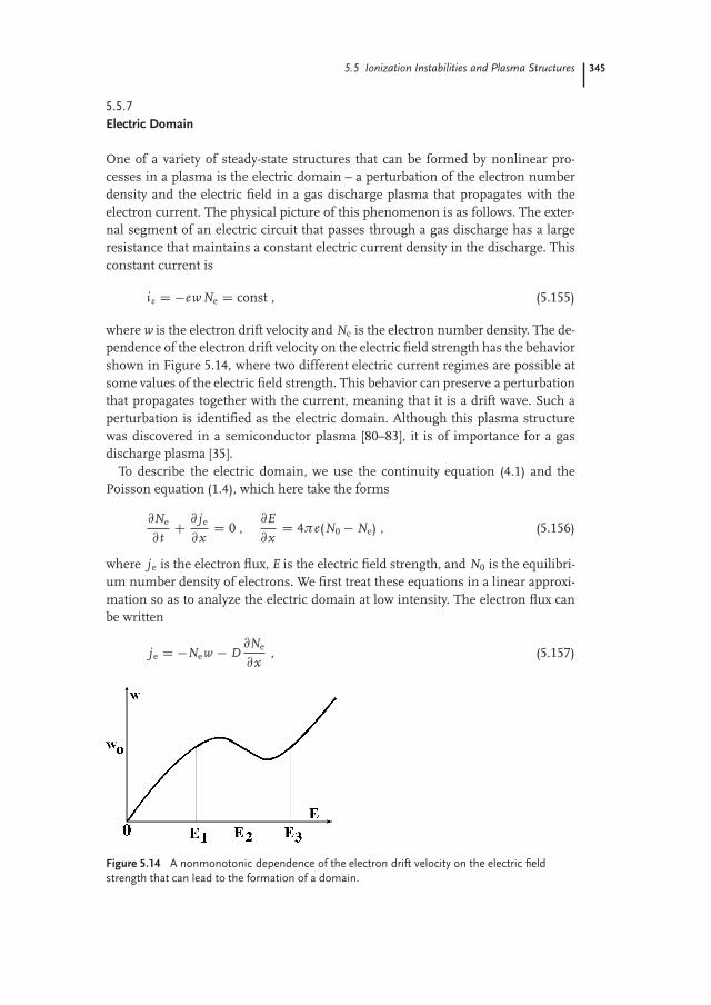
5.5 Ionization Instabilities and Plasma Structures 345
5.5.7
Electric Domain
One of a variety of steady-state structures that can be formed by nonlinear pro-cesses in a plasma is the electric domain – a perturbation of the electron numberdensity and the electric field in a gas discharge plasma that propagates with theelectron current. The physical picture of this phenomenon is as follows. The exter-nal segment of an electric circuit that passes through a gas discharge has a largeresistance that maintains a constant electric current density in the discharge. Thisconstant current is
ie D �ew Ne D const , (5.155)
where w is the electron drift velocity and Ne is the electron number density. The de-pendence of the electron drift velocity on the electric field strength has the behaviorshown in Figure 5.14, where two different electric current regimes are possible atsome values of the electric field strength. This behavior can preserve a perturbationthat propagates together with the current, meaning that it is a drift wave. Such aperturbation is identified as the electric domain. Although this plasma structurewas discovered in a semiconductor plasma [80–83], it is of importance for a gasdischarge plasma [35].
To describe the electric domain, we use the continuity equation (4.1) and thePoisson equation (1.4), which here take the forms
@Ne
@tC @ je
@xD 0 ,
@E@x
D 4πe(N0 � Ne) , (5.156)
where je is the electron flux, E is the electric field strength, and N0 is the equilibri-um number density of electrons. We first treat these equations in a linear approxi-mation so as to analyze the electric domain at low intensity. The electron flux canbe written
je D �New � D@Ne
@x, (5.157)
Figure 5.14 A nonmonotonic dependence of the electron drift velocity on the electric field
strength that can lead to the formation of a domain.
346 5 Waves, Instabilities, and Structures in Excited and Ionized Gases
where D is the diffusion coefficient of electrons in a plasma, and the minus sign inthe first term accounts for the direction of the electron current. Taking E and Ne toexhibit harmonic behavior as expressed by (5.48), we can write
E D E0 C E 0e i(k x�ω t ) , Ne D N0 C N 0e i(k x�ω t ) .
We then obtain the dispersion relation
ω D �kw � i D k2 � i � 4πN0edwdE
(5.158)
on the basis of (5.156) and (5.157) using the connection @w/@x D (dw/dE ) (dE/dx ). Dispersion relation (5.158) describes drift waves (5.129) that move to-gether with the electron current. The diffusion process removes electrons from theperturbation zone, thus causing damping of these waves. But if dw/dE < 0, longdrift waves with D k2 < i4πN0edw/dE can develop.
We now study a nonlinear electric domain. In a nonsteady interval of the electricfield strengths in Figure 5.14, (5.157) has the form
j0 D �N0w (E2) D �New (E ) � D@Ne
@x.
We should add to this equation the Poisson equation (1.4) or (5.156). Eliminatingthe electron number density between these equations, we obtain
Dd2Edx2 D w (E )
dEdx
� 4πeN0[w (E ) � w (E2)] . (5.159)
Equation (5.159) describes the behavior of the electric field strength in the electricdomain.
When we assume that diffusion plays a secondary role, and ignore diffusion inthe first stage of the analysis, (5.159) takes the form
dEdx
D 4πeN0
�w (E2)w (E )
� 1�
. (5.160)
We solve this equation with the boundary condition E D E2 atx D 0. The solutionis shown in Figure 5.15a. As follows from (5.160), E(x ) increases with x until E2 <
E < E3, where w (E3) D w (E2). At E D E3 we have dE/dx D 0, so for subsequentvalues of x we obtain E D E3. Thus, this solution describes the conversion of thesystem from the unstable state E2 to the stable state with E D E3.
This transition means that the change of the discharge regime as a result ofthe perturbation leads to an increase of the electric field strength up to E3. Thiswould require a variation of the discharge voltage, which is impossible because thedischarge voltage is maintained by the external voltage. Therefore, the variation ofthe electric field strength from E2 to E3 is a perturbation that takes place in a limitedregion of the plasma. A return to the initial value of the field occurs as a result ofdiffusion, leading to decay of the perturbation. Hence, a typical size of the back

5.5 Ionization Instabilities and Plasma Structures 347
Figure 5.15 The distribution of the electric field (a) and the electron number density (b) in the
electric domain.
boundary zone of the electric domain is of the order of D/w . The forward boundaryzone size can be estimated from (5.160), and is Δx D ΔE/(4πeN0Δw ), whereΔE D E3 � E2 and Δw D w (E2) � wmin (see Figure 5.14). A concomitant of thedistribution of the electric field strength in the electric domain is the distributionof the electron number density that is shown in Figure 5.15b and follows from thePoisson equation (5.156).
5.5.8
Striations as Ionization Waves
Striations or strates are plasma structures that are observed in a positive column ofa gas discharge of low or moderate pressure [84–89]. The column is striped in analternation of luminous and dark regions. Striations have a rich history of study,and a detailed description of some aspects of this phenomenon was made in thenineteenth century [90–94]. Thomson [95, 96] was the first to describe the oscilla-tions of the positive column of a gas discharge, and his equations were improvedby Druuyvesteyn [97, 98]. These oscillations may be considered as standing waves– stationary striations. Striations can be at rest or move to electrodes from the pos-itive column. In addition, striations may be self-induced oscillations or may beexcited by an external source [99–101]. In both cases they characterize wave prop-erties of a gas discharge plasma. Striations exist only in certain ranges of currentsand pressures, although this range may be wide enough. For example, in hydrogen,striations exist in the pressure range which varies within the limits of eight ordersof magnitude and in the range of discharge currents that covers four orders of

348 5 Waves, Instabilities, and Structures in Excited and Ionized Gases
magnitude [101]. Striations have different properties for atomic and for moleculargases.
Striations are ionization waves and may be considered as plasma structures re-sulting from an instability of ionization and recombination processes or as nonlin-ear ionization waves [61, 102]. From this standpoint, striations exist if a stratifiedplasma structure is more favorable than the uniform plasma distribution, that is,the electric voltage for a stratified structure of a gas discharge plasma at a givenelectric current corresponds to a lower voltage for gas discharge than that for auniform plasma [103]. Then in considering striations as an ionization instabili-ty [85, 86, 104–106], one can understand the conditions under which these ioniza-tion waves exist.
It is clear that if the ionization rate is independent of the electron number densi-ty, we obtain a stable uniform plasma, and for existence of an ionization instabilitythe above dependence is necessary. We now consider ionization waves in a plasmaresulting from stepwise ionization of atoms. This mechanism corresponds to low-pressure glow discharges in inert gases, where metastable atoms are of importancefor ionization processes, and below we will be guided by this case. Hence, from thestandpoint of the classification of striation types [107–109], we analyze below therange of low discharge currents. Along with ionization processes, we consider theambipolar diffusion that leads to loss of electrons and provides the stabilization ofa gas discharge plasma. The balance equation for the electron number density is
@Ne
@tC Da
@2Ne
@x2 D Z Ne , (5.161)
where Da is the ambipolar diffusion coefficient, the x-axis is along the axis of thedischarge tube, and Z is the sum of the rates of generation and loss of electrons.Assuming that the ionization wave has a small amplitude, we have the usual har-monic dependence Ne D N0 C N 0 exp(i k x � i ω t), where N 0 � N0. When weintroduce the effective electron temperature Te D T0 C T 0 exp(i k x � i ω t) andinsert these relations into (5.159), we obtain the dispersion relation [110]
ω D �i Dak2 C i ZT Ne@Te
@NeC i ZN Ne (5.162)
for the ionization wave, where we have used the notation ZN D @Z/@Ne and ZT D@Z/@Te, and have taken into account that Z D 0 at equilibrium.
This dispersion relation was obtained by a formal procedure. It is of importancethat the ionization rate Z depends on both the number density and the temperatureof the electrons, and variation of one of these quantities alters the other. Depend-ing on the connection between these quantities, waves can be either developed ordamped. We give some illustrative examples. Assume that the resistance of the ex-ternal circuit is large enough to conserve the electron current density i. Then wehave
i D Σ E C eDar Ne D const .
5.5 Ionization Instabilities and Plasma Structures 349
This gives the electric field
E D iΣ
� eDar Ne
Σ, (5.163)
where Σ is the plasma conductivity and Da is the coefficient of ambipolar diffusionthat characterizes the diffusion of electrons in a plasma.
When we use the balance equation for the mean energy of electrons, and takeinto account elastic collisions of electrons and gas atoms, the heat balance equationfor electrons has the form
div q D i � E � Neνδε D 0 , (5.164)
where q is the heat flux. The first term on the right-hand side of this equation ac-counts for heating of electrons under the action of the electric current. The secondterm takes into account elastic electron–atom collisions; ν is the collision rate andδε is the mean energy transferred to atoms in a single collision. Further, we as-sume that δε is proportional to the mean electron energy and that the collisionrate is independent of the electron energy.
We assume that the heat flux q is determined by the electron thermal conductivity(q D ��r Te, where � is the thermal conductivity coefficient of electrons) andΣ � Ne . Taking the values Σ and Da to be dependent on Te, (5.163) and (5.164)give the dispersion relation
k2�T 0 D � i2
ΣN 0
N0� i kE j Da
ΣN 0 � i2
ΣN 0
N0C T 0
T0.
From this it follows that
@Te
@NeD T 0
N 0D T0
N0
(�2 � i k/ k0)(1 C k2/ k2
1 ), (5.165)
where k0 D i/(eDaN0) and k1 D ip
Σ T0�. On the basis of (4.40) we have theestimate for the thermal conductivity coefficient due to electrons � � N0ve λ, andfrom (3.42) we have Σ � N0e2λ/(meve), where N0 is the equilibrium electronnumber density and ve � p
Te/me is a typical thermal electron velocity. From thiswe conclude that k0 and k1 have the same order of magnitude.
We now find the conditions that will give rise to an ionization instability lead-ing to the formation of striations. For this goal we substitute (5.165) into (5.162)and analyze the resulting expression. Since the effective electron temperature Te issmall compared with the atomic ionization potential J/Te � J , (3.69) and (3.70)give ZT � ( J/T 2
e )νion, where νion is the rate of atom ionization by electron im-pact. Because of the dependence of Z on the electron number density, we haveZN � νion/N0. This gives ZN N0 � ZT Te, and for long-wave oscillations (k � k0),(5.162) and (5.165) give Im ω < 0, so long-wave oscillations are damped. There-fore, striations as nonlinear ionization waves can only be short-wave oscillations.Then the criterion for the existence of striations (the Rother condition [111–113])has the form
ZN > 0 . (5.166)
350 5 Waves, Instabilities, and Structures in Excited and Ionized Gases
There is a range of wavelengths satisfying the condition k > k0, where Re ω >
Im ω, so ionization waves – striations – can exist. These waves are developed bynonlinear interaction processes.
Consider the example of ionization instability, governed by the nonlinear step-wise ionization of atoms by electron impact. We shall assume that there is only oneexcited atomic state that contributes to the ionization. We denote this state by thesubscript or superscript �. We thus have
Z D Nakion C N�k�ion � 1/τD , (5.167)
where Na and N� are the atom number densities in the ground and excited states,kion and k�
ion are the rate constants for ionization of atoms in the ground and excitedstates caused by electron impact, and τD is the time for diffusion of electrons to thewalls of the discharge tube. At equilibrium we have Z D 0. The dependence of Zon the electron number density due to ionization of excited atoms is
ZN D k�ion
@N�
@Ne. (5.168)
Using (3.66) for the number density of excited atoms, we obtain
N� D N B�
�1 C 1
Ne kqτD
��1
,
where N B� is given by the Boltzmann formula and corresponds to equilibrium be-
tween the ground and excited states. Substituting this into (5.165) and (5.166), andusing the relation n� D 1/(kq τD), we have
ZN D k�ion n�N B
�
(Ne C n�)2 , ZT D JT 2
e
�kion Na C kion N B
� Ne
Ne C n�
�.
Inserting these expressions into (5.160) yields
Re ω D �I m�
ZT Ne@Te
@Ne
�D J
T 2e
�kion Na C kionN B
� Ne
Ne C n�
�k/ k0
1 C k2/ k21
,
Im ω D k�ion n�N B
� Ne
(Ne C n�)2� Dak2 � 2 J
T 2e
�kion Na C kionN B
� Ne
Ne C n�
�1
1 C k2/ k21
(5.169)
for the frequency and damping (or amplification) of the ionization wave, where k0
and k1 are defined in (5.165).Equations (5.169) identify that range of parameters where amplification of
the ionization wave (Im ω > 0) can occur. According to (3.69), we find thatkionNa/(k�
ion N B�) � J�/ J < 1, where J and J� are the ionization potentials of the
atom in the ground and excited states. Hence, when Ne � N� and k > k1( J/Te),the last term in expressions (5.169) for the growth of the ionization wave is notcompensated for by the first term. Then the ionization wave can develop until it

5.5 Ionization Instabilities and Plasma Structures 351
will no longer decay as a result of electron diffusion. Thus, the ionization wave canamplify in the range of wave vectors
k1
sJ
Te< k <
skion N B
�
Da. (5.170)
If this condition is satisfied, ionization waves can develop, and striations arise. Theplasma then exhibits a striped structure with a specific periodicity.
Considering the striations as ionization waves gives an understanding of someaspects of this problem [85, 86]. One can formulate conclusions which follow fromthe above analysis of striations as instabilities of ionization waves in a gas dischargeplasma. For low gas discharge currents this instability proceeds only in an interme-diate range of electron number densities where the ionization rate depends on thenumber density of electrons (the Rother condition (5.166)). Next, we have differ-ent regions in the spatial distributions of species, so the wave distribution of theelectron number density is shifted with respect to the electron temperature.
5.5.9
Self-Consistent Structure of Striations
In considering striations as ionization waves, we divide a region into elements withthe length of a wave for each element, so plasma parameters are repeated in eachelement. According to the Pupp classification [107–109], for striations of low pres-sure and discharge electric currents, the wavelengths of striations as oscillationsin a plasma of inert gases are small compared with the mean free path electronswith respect to energy change in elastic electron–atom collisions, but are large incomparison with the mean free path of electrons with respect to electron scatteringby atoms. According to the properties of waves, the electric voltage '(λ) betweentwo points a distance of one wave period λ apart is the same
'(λ) DλZ
0
E(x )dx D const ,
where E(x ) is the electric field strength at point x and λ is the wavelength forstriations. According to the Novak rule [116], the voltage per striation is almostconstant for a given striation type, that is, this value is independent of the electriccurrent and pressure. As a demonstration of this, Table 5.1 gives the values of thevoltage per striation for three striation types (P, R, S) in gas discharge of inert gases,where these values are compared with the atomic excitation energy ΔE , the atomicionization potential J and the ionization potential J� for a metastable atom.
Our goal is to understand the nature of striations as ionization waves in an atom-ic gas of low density if the mean free path of electrons is small compared with astriation length (the spatial period of oscillations), but the mean free path of elec-trons with respect to variation of their energy as a result of elastic collisions with

352 5 Waves, Instabilities, and Structures in Excited and Ionized Gases
Table 5.1 The electric potential (V) on one striation for three types of striations in inert gas-
es [86]. The atomic excitation energy ΔE is given along with the atomic ionization potential in
the ground J and metastable J� states.
Types of striation P R S ΔE , eV J, eV J�, eV
He 14.2 – 30.05 19.8 24.6 4.8Ne 9.2 12.7 19.5 16.62 21.5 4.9
Ar 6.7 9.5 12.0 11.55 15.76 4.2
atoms exceeds the striation length significantly. Under these conditions, the varia-tion of the electron energy as a result of the electron displacement from coordinatex1 to coordinate x2 along the field is [114, 115]
ε(x1) C '(x1) D ε(x2) C '(x2) ,
where ε is the electron energy at an indicated point and ' is the plasma electricpotential at this point. Hence, in the first approximation each electron acquires acertain energy after passage of one striation.
Let us combine this with the Novak rule [116], according to which the energyacquired by an electron after passage of one striation period is constant for a givenstriation type, that is, it is independent of the gas pressure and discharge current.One can conclude from this that a certain energy is given to an individual elec-tron on each striation. On this basis one can construct a certain physical picture ofplasma processes with formation of striations. Indeed, if a group of electrons lose
Figure 5.16 Distributions of the number density of electrons (a) and the electric field strength
(b) along a gas discharge tube of small radius under the formation of striations.

5.5 Ionization Instabilities and Plasma Structures 353
excitation energy, these electrons are stopped, and their density increases in a cor-responding point of space (see Figure 5.16). Then the voltage distribution in spacehas the form of a “Tsendin staircase”, as shown in Figure 5.17 [89, 117]. Moreover,Figure 5.17 shows the bunching of the electron flux in this case. Indeed, each elec-tron that partakes in excitation loses an identical amount of energy, and for theseelectrons in this approximation the electron energy distribution function is con-served on the following striation. If we take into account the energy loss in elasticelectron–atom collisions, fast electrons lose more high energy than slow ones. As aresult, the electron energy distribution function becomes narrower, and bunchingof electrons takes place. Within the framework of this description, one can expectformation of striations in the case when two regimes of the plasma state, with stri-ations and for the uniform plasma distribution, may be realized. Then one canconsider a plasma with striations as an energetically profitable plasma state [103],that is, in this plasma state the total voltage of this plasma is optimal.
Seemingly, the Tsendin model, which is based on a stronger braking of fastelectrons compared with slow ones, allows us to explain the nature of striationformation. Indeed, the electron velocity distribution function is narrow owing tobunching of the electron beam and is not broadened after passage of many striationperiods. Then the energy
λZ0
eE(x )dx D Δε (5.171)
Figure 5.17 Tsendin staircase – the form of the plasma potential in striation formation and the
character of bunching [89, 117].

354 5 Waves, Instabilities, and Structures in Excited and Ionized Gases
obtained by an individual electron after passage of one period subsequently goesinto atom ionization. Equation (5.171) holds in the absence of energy exchange be-tween electrons and atoms as a result of elastic collisions, and in the absence ofelectron–electron collisions. Evidently, the energy Δε is equal to e', where ' is theelectric voltage on one striation given in Table 5.1 for inert gases. For example, onecan expect Δε to be equal to or close to the atomic excitation energy for striations ofa certain type. Then collision of two excited atoms formed after this striation leadsto ionization. Unfortunately, we do not have a direct connection between the val-ues in Table 5.1 and the atomic excitation energies or atomic ionization potentials.This testifies also to the role of metastable atoms in ionization processes involvingstriations.
Nevertheless, if we overlook this contradiction, we can come to an agreementabout the character of variation of striation parameters in this model with thePekarek theory [86, 104–106]. Indeed, at the beginning of some striation, wherethe electrons are slow, the number density of electrons is higher than that in a re-gion of fast electrons because their flux in the longitudinal direction is conserved.Hence, the regions of the maximum number density and the maximum energy(temperature) of electrons (or glowing maximum) are shifted in accordance withthe above-mentioned theory. Note that along with ionization processes, the loss ofelectrons and ions takes place as a result of their ambipolar diffusion to walls. Weassume there are long striations in a discharge tube if the tube radius is small com-pared with the striation wavelength, so the loss process proceeds uniformly alongthe tube.
In conclusion of this analysis, we note that the striation mechanism under con-sideration corresponds to low pressures in atomic gases, which allows us to ignorethe energy loss of electrons in elastic collisions with atoms. Next, we ignore elec-tron–electron collisions, so the discharge currents for this mechanism of striationsare limited. Under such conditions, the energy transferred to electrons from theelectric field of the discharge is consumed in excitation and ionization of atoms.Because striations exist for a nonlinear dependence of the ionization rate on thenumber density of electrons, the ionization process in a striated plasma has astepwise character. From this it follows that metastable atoms are of importancefor generation of striations in inert gases, and along with electron collisions withmetastable atoms, diffusion of metastable atoms in a plasma may be important forformation of striations. The latter process leads to washing out of the striation wavein contrast to the above-mentioned bunching mechanism.
This model shows that two regimes of the plasma can exist. In the first, the plas-ma is homogeneous, and ionization of atoms by electron impact occurs throughoutthe plasma. In the other regime, ionization occurs in narrow ionization zones dis-tributed periodically over the length of the discharge tube. That is, striations existin this regime. The regime in which the discharge plasma finds itself is determinedby the energy available to the system, so the characteristics of an external source ofelectricity are of great importance for the plasma behavior.

References 355
References
1 Landau, L.D. and Lifshits, E.M. (1959)Fluid Mechanics, Pergamon Press, Lon-don.
2 Batchelor, G.K. (1967) An Introduction toFluid Dynamics, Cambridge UniversityPress, Cambridge.
3 Drazin, P. and Reid, W. (1981) Hydro-dynamic Stability, Cambridge UniversityPress, Cambridge.
4 Acheson, D.J. (1990) Elementary Flu-id Dynamics, Oxford University Press,Oxford.
5 Lord Rayleigh (1916) Philos. Mag., 32,529.
6 Gershuni, G.Z. and Zhukhovitskii, E.M.(1972) Convective Stability of CompressedLiquid, Nauka, Moscow, in Russian.
7 Benard, H. (1900) Rev. Gen. Sci. PureAppl., 11, 261.
8 Benard, H. (1900) Rev. Gen. Sci. PureAppl., 11, 1309.
9 Benard, H. (1901) Ann. Chim. Phys., 23,62.
10 Chandrasekhar, S. (1961) Hydrodynam-ic and Hydromagnetic Stability, OxfordUniversity Press, London.
11 Koschmieder, E.L. (1993) Benard Cellsand Taylor Vortices, Cambridge Universi-ty Press, Cambridge.
12 Getting, A.V. (1998) Rayleigh–Taylor Con-vection Structure and Dynamics, WorldScientific Publishing, London.
13 Nernst, W. (1918) Z. Electrochem., 24,335.
14 Semenov, N.N. (1928) Z. Phys., 48, 571.15 Zeldovich, Ya.B. and Frank-
Kamenestkii, D.A. (1938) Zh. Fiz. Khim.,12, 100.
16 Zeldovich, Ya.B. and Frank-Kamenestkii, D.A. (1938) Dokl. Akad.Nauk SSSR, 19, 693.
17 Arrhenius, S. (1889) Z. Phys. Chem., 4,226.
18 Laidler, K.J. (1993) The World of Physi-cal Chemistry, Oxford University Press,Oxford.
19 Levine, R.D. (2005) Molecular ReactionDynamics, Cambridge University Press,Cambridge.
20 Zeldovich, Ya.B. (1944) Theory of Com-bustion and Gas Detonation. Izdat. ANSSSR, Moscow, in Russian.
21 Frank-Kamenestkii, D.A. (1969) Dif-fusion and Heat Transfer in ChemicalKinetics, Plenum Press, New York.
22 Kondrat’ev, V.N. and Nikitin, E.E. (1974)Kinetics and Mechanism of Gas-PhaseReactions, Nauka, Moscow, in Russian.
23 Zeldovich, Ya.B., Barenblatt, G.I., Li-brovich, V.B., and Makhviladze, G.M.(1985) The Mathematical Theory of Com-bustion and Explosions, Consultants Bu-reau, New York.
24 Stix, T.H. (1992) Waves in Plasmas, Amer-ican Institute of Physics, New York.
25 Swanson, D.G. (2003) Plasma Waves,Institute of Physics Publishing, Bristol.
26 Langmuir, I. (1925) Phys. Rev., 26, 585.27 Langmuir, I. (1928) Proc. Natl. Acad. Sci.
USA, 14, 627.28 Tonks, L. and Langmuir, I. (1929) Phys.
Rev., 33, 195.29 Bohm, D. and Gross, E.P. (1949) Phys.
Rev., 75, 1851.30 Bohm, D. and Gross, E.P. (1949) Phys.
Rev., 75, 1864.31 Alfvén, H. (1942) Nature, 150, 405.32 Alfvén, H. (1950) Cosmical Electrodynam-
ics, Oxford University Press, London.33 Landau, L.D. and Lifshitz, E.M. (1960)
Electrodynamics of Continuous Media,Pergamon Press, Oxford.
34 Alfvén, H. and Fälthammar, C.G. (1963)Cosmical Electrodynamics. FundamentalPrinciples, Clarendon Press, London.
35 Kadomtsev, B.B. (1988) Cooperative Phe-nomena in Plasma, Nauka, Moscow,in Russian,English version: Shafra-nov, V.D. (2001) Rev. Plasma Phys., 22,1.
36 Fälthammar, C.G. (1963) Cosmic Elec-trodynamics. Fundamental Principles,Clarendon Press, London.
37 Ginzburg, V.L. and Rukhadze, A.A.(1972) Waves in Magnetoactive Plasma,Nauka, Moscow, in Russian.
38 Maxwell, J.C. (1865) Philos. Trans. Phys.Soc., 155, 459.

356 5 Waves, Instabilities, and Structures in Excited and Ionized Gases
39 Maxwell, J.C. (1873) Treatise on Electric-ity and Magnetism, Oxford University,London.
40 Heaviside, O. (1884) Electrician, 12, 583–586.
41 Thomson, J.J. (1928) Proc. Phys. Soc., 40,82.
42 Faraday, M. (1846) Philos. Trans. R. Soc.,136, 1.
43 Faraday, M. (1859) Experimental Re-searches in Chemistry and Physics, Taylorand Francis, London.
44 VanVleck, J.H. (1932) The Theory of Elec-tric and Magnetic Susceptibilities, OxfordUniversity Press, New York.
45 Born, M. (1933) Optik, Springer, Berlin.46 Jenkins, F.A. and White, H.E. (1976)
Fundamentals of Optics, McGraw-Hill,New York.
47 Wood, R.W. (1988) Physical Optics, Opti-cal Society of America, Washington.
48 Mansuripur, M. (1995) The PhysicalPrinciples of Magneto-optical Recording,Cambridge University Press, London.
49 Piece, W.H (1894) Nature, 49, 554.50 Barkhausen, H. (1919) Phys. Z., 20, 401.51 Helliwell, R.A. (1965) Whistlers and Re-
lated Ionospheric Phenomena, StanfordUniversity Press, Stanford.
52 Akhiezer, A.I. and Feinberg, Ya.B. (1951)Zh. Eksp. Teor. Fiz., 21, 1262.
53 Gabor, D., Ash, E.A., and Dracot, D.(1955) Nature, 178, 916.
54 Nezlin, M.V. (1995) Physics of IntenseBeams in Plasmas, IOP Publishing, Bris-tol.
55 Buneman, O. (1958) Phys. Rev. Lett., 1, 8.56 Buneman, O. (1963) Phys. Rev. Lett., 10,
285.57 Khalil, S.H.M. and Mohamed, B.F.
(1991) Contrib. Plasma Phys., 31, 513.58 Benett, W.H. (1934) Phys. Rev., 45, 890.59 Mikhailowskii, A.B. (1974) Theory of
Plasma Instabilities, Consultant Bureau,New York.
60 Mikhailovskii, A.B. (1992) Electromag-netic Instabilities in an InhomogeneousPlasma, IOP Publishing, Bristol.
61 Landa, P.C. (2010) Nonlinear Oscillationsand Waves in Dynamical Systems, Kluwer,Dordrecht.
62 Kadomtzev, B.B. (1965) Plasma Turbu-lence, Academic Press, New York.
63 Tsytovich, V.N. (1970) Nonlinear Effectsin Plasmas, Plenum Press, New York.
64 Hasegawa, A. (1975) Plasma Instabilitiesand Nonlinear Effects, Springer, Berlin.
65 Wojaczek, K. (1962) Beitr. Plasmaphys.,2, 1.
66 Lighthill, M.J. (1965) J. Inst. Math. Appl.,1, 1.
67 Korteweg, D.J. and de Vries, G. (1895)Philos. Mag., 39, 422.
68 Stenzel, R., Kim, H.C., and Wong, A.Y.(1974) Phys. Rev. Lett., 32, 659.
69 Ikezi, H., Nishikawa, K., and Mima, K.(1974) J. Phys. Soc. Jpn., 37, 766.
70 Antipov, S.V. et al. (1976) JETP Lett., 23,562.
71 Antipov, S.V. et al. (1977) JETP Lett., 25,145.
72 Antipov, S.V. et al. (1981) Physica D, 3,311.
73 Thejappa, G. et al. (1999) J. Geophys.Res., 104, 279.
74 Ivanov, A.A. (1977) Physics of Strong-ly Nonequilibrium Plasma, Atomizdat,Moscow, in Russian.
75 Das, K.P. and Sihi, S. (1982) Plasma-physics, 22, 29.
76 Agrawal, G.P. (1995) Nonlinear FiberOptics, Academic Press, San Diego.
77 Eletskii, A.V. (1986) Sov. Phys. JTP, 56,850.
78 Nedospasov, A.V. (1975) Sov. Phys. Usp.,18, 588.
79 Khalil, S.H.M., Sayee, Y.A., and Za-ki, N.G. (1989) Contrib. Plasma Phys., 29,605.
80 Gunn, J.B. (1963) Solid State Commun.,1, 88.
81 Gunn, J.B. (1965) Int. Sci. Technol., 46,43.
82 Bonch-Bruevich, V.L., Zvyagin, I., andMironov, A. (1972) Domain Electric Insta-bility in Semiconductors, Nauka, Moscow,in Russian.
83 Pozhela, J. (1981) Plasma and CurrentInstabilities in Semiconductors, PergamonPress, Oxford.
84 Oleson, N.L. and Cooper, A.W. (1968)Adv. Electron. Electron Phys., 1, 65.
85 Nedospasov, A.V. (1968) Sov. Phys. Usp.,11, 174.
86 Pekarek, L. (1968) Sov. Phys. Usp., 11,188.

References 357
87 Garscadden, A. (1978) in Gaseous Elec-tronics, (eds. M.N. Hirsh, H.J. Oskam),Academic Press, New York p. 1, 65.
88 Kolobov, V.I. (2006) J. Phys. D, 39, R487.89 Tsendin, L.T. (2010) Phys. Usp., 180, 130.90 Wüllner, A. (1874) Ann. Phys. Chem., 32,
1.91 Spottiswoode, W. (1875) Proc. R. Soc.,
23, 455.92 Spottiswoode, W. (1876) Proc. R. Soc.,
24, 73.93 Spottiswoode, W. (1877) Proc. R. Soc.,
25, 547.94 Spottiswoode, W. (1877) Proc. R. Soc.,
26, 90.95 Thomson, J.J. (1921) Philos. Mag., 42,
1454.96 Thomson, J.J. and Thomson, G.P. (1933)
Conduction of Electricity through Gases,Cambridge University Press, London.
97 Druyvesteyn, M.J. (1934) Physica, 1, 273.98 Druyvesteyn, M.J. (1934) Physica, 1,
1003.99 Zaitsev, A.A. (1951) Dokl. Akad. Nauk
SSSR, 79, 779, in Russian.100 Zaitsev, A.A. (1952) Dokl. Akad. Nauk
SSSR, 84, 41, in Russian.
101 Klarfel’d, B.N. (1952) Zh. Teor. Exp. Fys.,22, 6.
102 Landa, P.C., Miskinova, N.A., and Pono-marev, Yu.V. (1990) Sov. Phys. Usp. 22,813.
103 Raizer, Yu.P. (1997) Gas DischargePhysics, Springer, Berlin.
104 Pekarek, L. (1954) Czech. J. Phys., 4, 221.105 Pekarek, L. (1957) Phys. Rev., 108, 1371.106 Rohlena, K., Ruzicka, T., and Pekarek, L.
(1972) Czech. J. Phys. B, 22, 72.107 Pupp, W. (1932) Phys. Z., 33, 844.108 Pupp, W. (1933) Phys. Z., 34, 756.109 Pupp, W. (1934) Phys. Z., 35, 705.110 Wojaczek, K. (1959) Monatsber. Dtsch.
Akad. Wiss., 1, 23.111 Rother, H. (1959) Ann. Phys., 4, 373.112 Rother, H. (1959) Z. Phys., 157, 326.113 Rother, H. (1960) Ann. Phys., 5, 252.114 Bernstein, I.B. and Holstein, T. (1954)
Phys. Rev., 94, 1475.115 Tsendin, L.T. (1974) Sov. Phys. JETP, 39,
805.116 Novak, M. (1960) Czech. J. Phys., 10, 954.117 Tsendin, L.T. (1995) Plasma Source
Sci.Technol. 4, 200.