fundamentals of gis ©2008 all lecture materials by austin troy except where noted lecture 10:...

Fundamentals of GIS

©2008 All lecture materials by Austin Troy except where noted

Lecture 10:Spatial Interpolation, geostatistics

and sampling

By Austin Troy

------Using GIS--

Fundamentals of GIS


What is interpolation?• Three types:

1. Resampling of raster cell size

2. Transforming a continuous surface from one data model to another (e.g. TIN to raster or raster to vector).

3. Creating a surface based on a sample of values within the domain.

Fundamentals of GIS


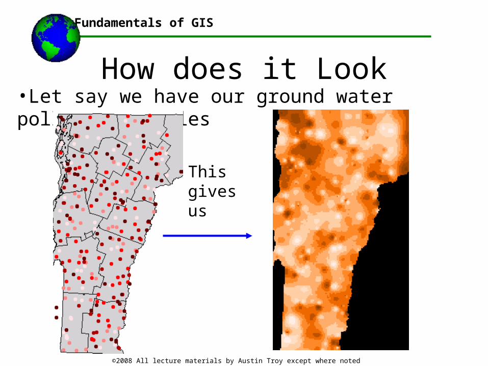
How does it Look•Let say we have our ground water pollution samples

This gives us

Fundamentals of GIS


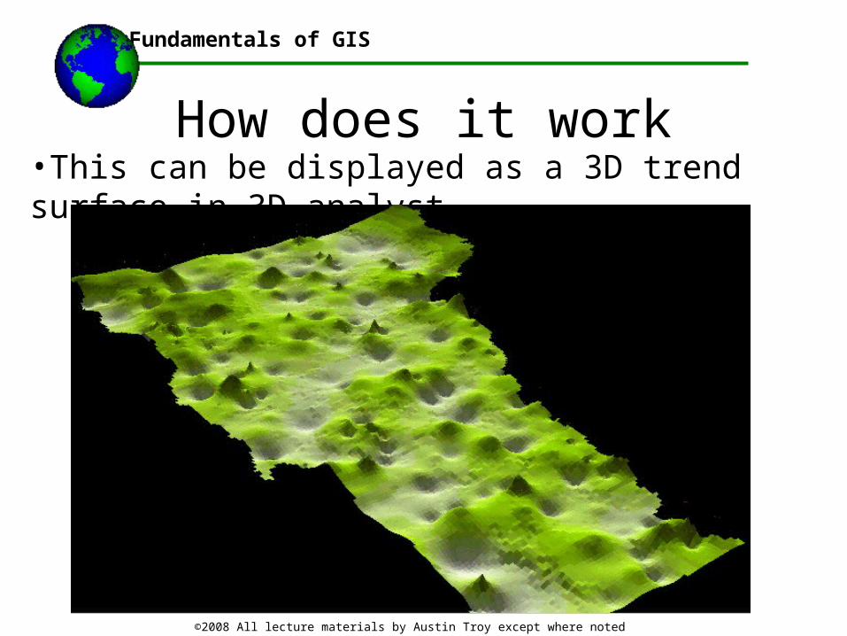
How does it work•This can be displayed as a 3D trend surface in 3D analyst

Fundamentals of GIS


Requirements of interpolation•Interpolation only works where values are spatially dependent—that values for nearby points tend to be more similar

•Where values across a landscape are geographically independent, interpolation does not work

Fundamentals of GIS


Interpolation examples•Elevation:

•Elevation values tend to be highly spatially autocorrelated because elevation at location (x,y) is generally a function of the surrounding locations

•Except is areas where terrain is very abrupt and precipitous, such as Patagonia, or Yosemite

•In this case, elevation would not be autocorrelated at local (large) scale, but still may be autocorrelated at regional (small scale)

Fundamentals of GIS


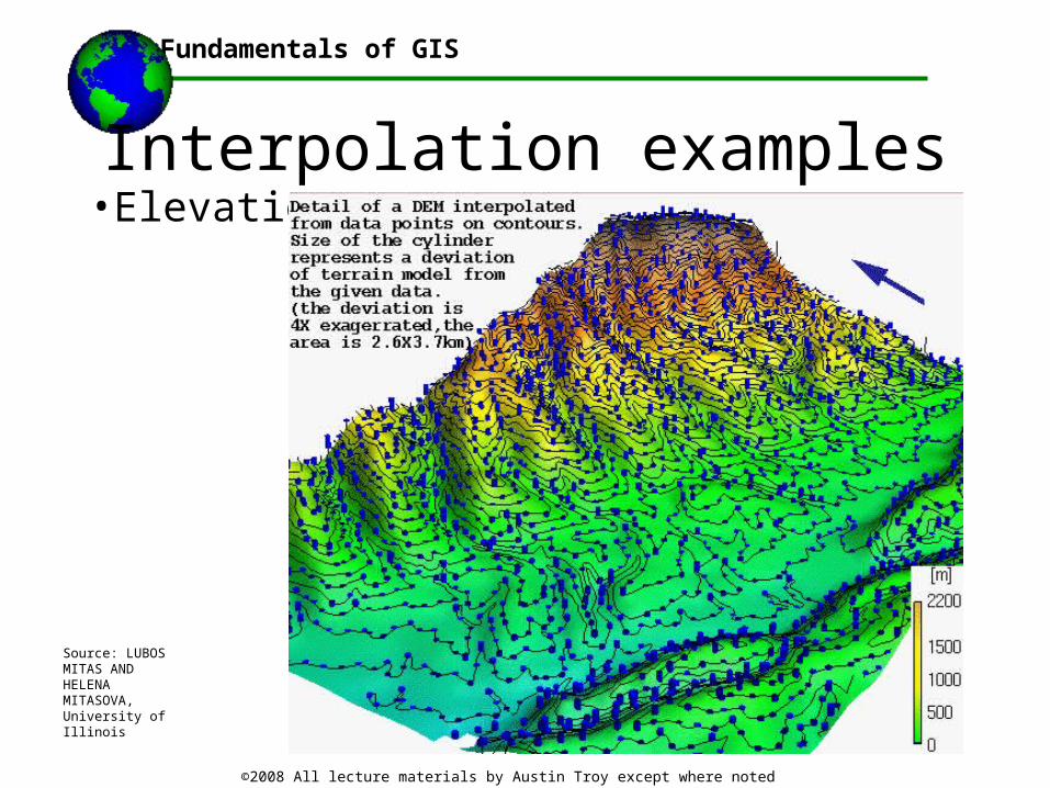
Interpolation examples•Elevation:

Source: LUBOS MITAS AND HELENA MITASOVA, University of Illinois

Fundamentals of GIS


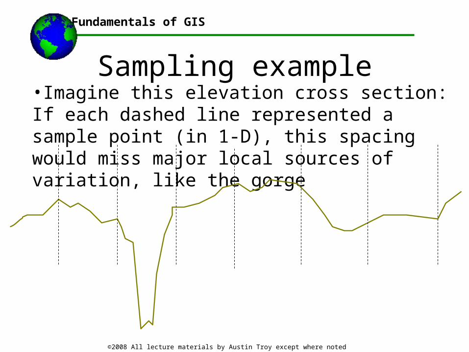
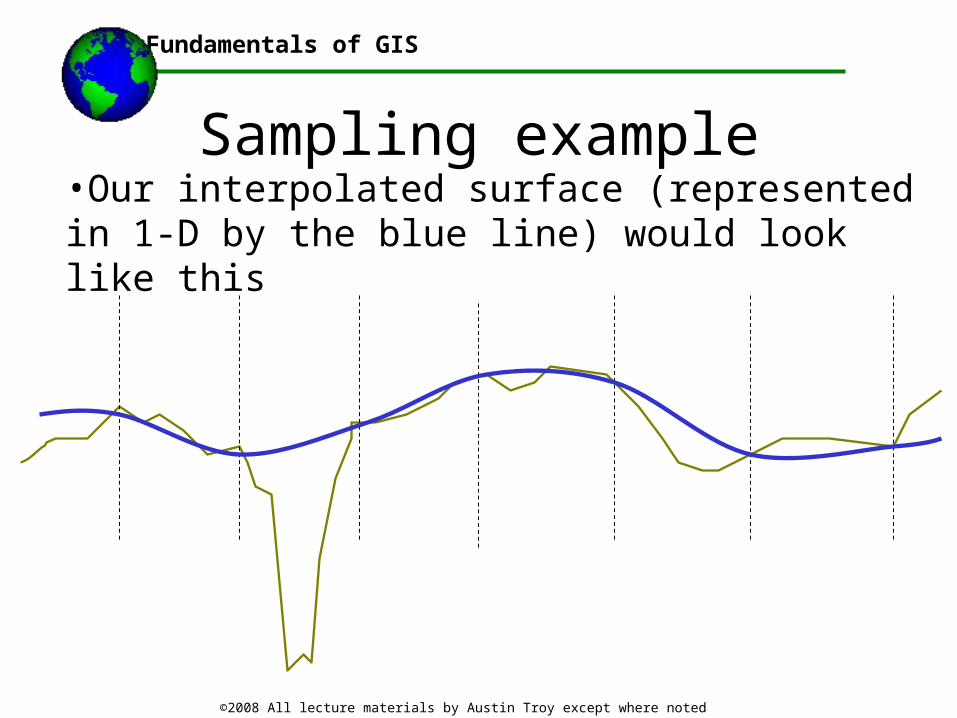
Sampling example•Imagine this elevation cross section: If each dashed line represented a sample point (in 1-D), this spacing would miss major local sources of variation, like the gorge

Fundamentals of GIS


Sampling example•Our interpolated surface (represented in 1-D by the blue line) would look like this

Fundamentals of GIS


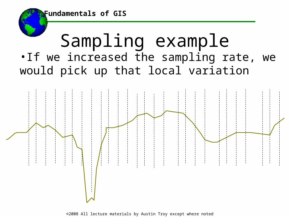
Sampling example•If we increased the sampling rate, we would pick up that local variation

Fundamentals of GIS


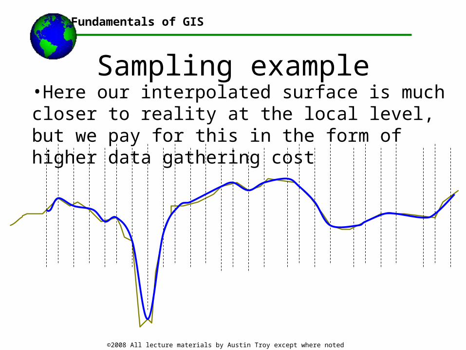
Sampling example•Here our interpolated surface is much closer to reality at the local level, but we pay for this in the form of higher data gathering cost

Fundamentals of GIS


Interpolation examples

•Weather: Great Plains vs SF Bay Area

•Groundwater contamination: depends on geology

•Crime rates: depends on population density

•New York City income: may require fine scale

Fundamentals of GIS


Sampling Approaches•Often a regular gridded sampling strategy is appropriate and can eliminate sampling biases

•Sometimes, though, it can introduce biases if the grid pattern correlates in frequency with something in the landscape, such as trees in a plantation or irrigation lines

•Random sampling can avoid this but introduces other problems including difficulty in finding sample points and uneven distribution of points, leading to geographic gaps.

•This depends partially on the size of the support, or sampling unit

Fundamentals of GIS


Sampling Approaches•An intermediate approach is the stratified random sample

•Create geographic or non-geographic subpopulations, from each of which random sample is taken

•Proportional or equal probability SRS: enforce a certain sampling rate, πhj= nh/Nh for each stratum h and obs j.

•Simple SRS: enforce a certain sample size nh

•Disproportionate SRS: where πhj varies such that certain strata are oversampled and certain undersampled.

Fundamentals of GIS


Sampling Approaches•DSRS is advantageous when subpopulation variances are unequal, which is frequently the case when stratum sizes are considerably different. In DSRS we sample those strata with higher variance at higher rate. We may also use this when we have an underrepresented subpopulation that will have too few observations to model if sampled with SSRS.

•Proportional samples are self-weighting because the rates are the same for each stratum

•The other two have unequal sampling probabilities (unless a simple SRS has equal Nh) and may require weighting

Fundamentals of GIS


Sampling Approaches•When the stratifying unit is geographical (e.g. county, soil polygon, forest stand), this is called a cluster sample.

•In a one stage cluster sample (OSCS) a series of geographic units are sampled and all observations within are sampled: obviously this does not work for interpolation

•More relevant is a two stage cluster sample (TSCS) in which we take a sample of cluster units and then a subsample of the population of each cluster unit.

•In this type of sample, variance has two components, that between clusters and that between observations

Fundamentals of GIS


Sampling•The number of samples we want within each zone depends on the statistical certainty with which we want to generate our surface

•Do we want to be 95% certain that a given pixel is classified right, or 90% or 80%?

•Our desired confidence level will determine the number of samples we need per strata

•This is a tradeoff between cost and statistical certainty

•Think of other examples where you could stratify….

Fundamentals of GIS


Sampling•A common problem with sampling points for interpolation is what is not being sampled?

•Very frequently people leave out sample points that are hard to get to or hard to collect data at

•This creates sampling biases and regions whose interpolated values are essentially meaningless

Fundamentals of GIS


Sampling example•Say we want to make an average precipitation layer and we find that in our study zone precipitation is highly spatially variable within 10 miles of the ocean

•We’d a coastline layer to help us sample.

•We’d have high density of sampling points within 10 miles of the ocean a much lower density in the inland zones

Fundamentals of GIS


Sampling example•Say we were looking at an inland area, far from any ocean, and we decided that precipitation varied with elevation. How would we set up our sampling design?

•In this case, flat areas would need fewer sample points, while areas of rough topography would need more

•In our sampling design we would set up zones, or strata, corresponding to different elevation zones and we would make sure that we get a certain minimum number of samples within each of those zones

•This ensures we get a representative sample across, in this case, elevation;

Fundamentals of GIS


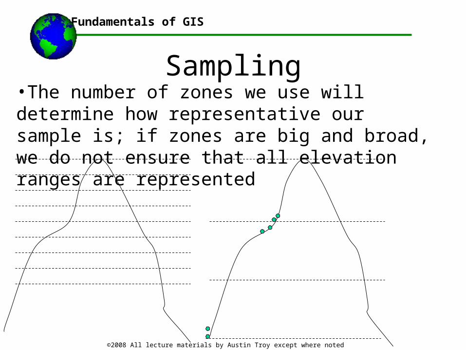
Sampling•The number of zones we use will determine how representative our sample is; if zones are big and broad, we do not ensure that all elevation ranges are represented

Fundamentals of GIS


Sampling and Scale dependency•Sampling strategy for interpolation depends on the scale at which you are working and the scale dependency of the phenomenon you are studying

•In many cases interpolation will work to pick up regional trends but lose the local variation in the process

•The density of sample points must be chosen to reflect the scale of the phenomenon you are measuring.

Fundamentals of GIS


Scale dependency•If you have a high density of sample points, you will capture local variation, which is appropriate for large-scale (small-area) studies

•If you have low density of sample points, you will lose sensitivity of local variation and capture only the regional variation; this is more appropriate for small-scale (large-area) studies

Fundamentals of GIS


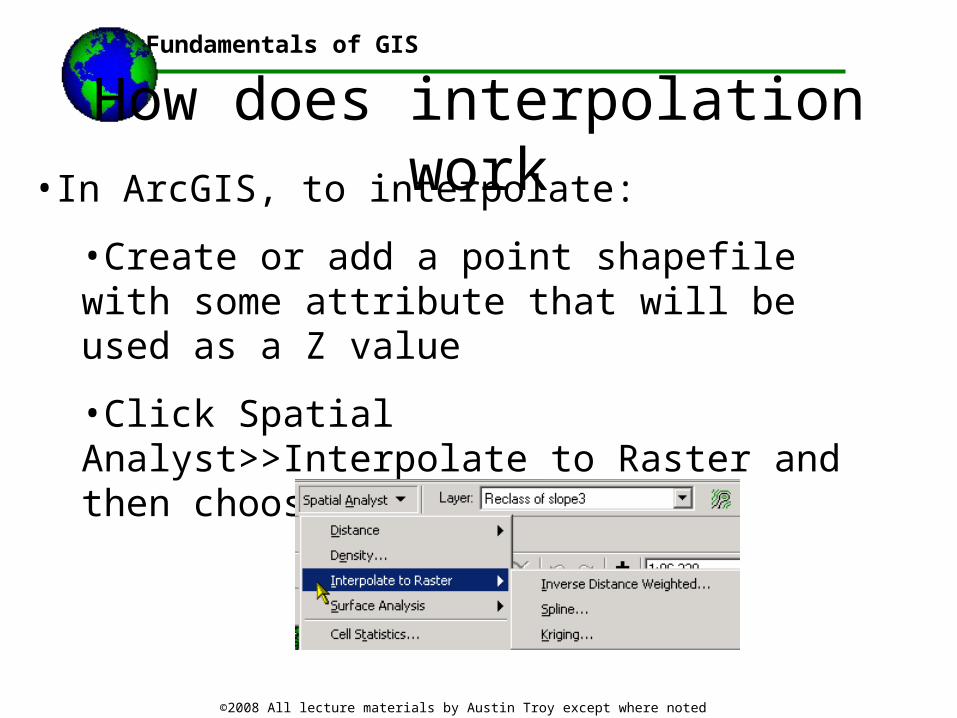
How does interpolation work•In ArcGIS, to interpolate:

•Create or add a point shapefile with some attribute that will be used as a Z value

•Click Spatial Analyst>>Interpolate to Raster and then choose the method

Fundamentals of GIS


Three methods in Arc GIS•IDW

•SPLINE

•Kriging

Fundamentals of GIS


Inverse Distance Weighting•IDW weights the value of each point by its distance to the cell being analyzed and averages the values.

•IDW assumes that unknown value is influenced more by nearby than far away points, but we can control how rapid that decay is. Influence diminishes with distance.

•IDW has no method of testing for the quality of predictions, so validity testing requires taking additional observations.

•IDW is sensitive to sampling, with circular patterns often around solitary data points

Fundamentals of GIS


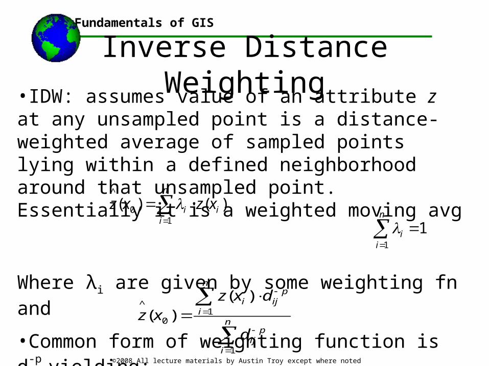
•IDW: assumes value of an attribute z at any unsampled point is a distance-weighted average of sampled points lying within a defined neighborhood around that unsampled point. Essentially it is a weighted moving avg

Where λi are given by some weighting fn and

•Common form of weighting function is d-p

yielding:

Inverse Distance Weighting

n

iii xzxz

10

^

)()(

n

ii

1

1

n

i

pij

n

i

piji

d

dxzxz

1

10

^)(

)(

Fundamentals of GIS


IDW-How it works

•Z value at location ij is f of Z value at known point xy times the inverse distance raised to a power P.

•Z value field: numeric attribute to be interpolated

•Power: determines relationship of weighting and distance; where p= 0, no decrease in influence with distance; as p increases distant points becoming less influential in interpolating Z value at a given pixel

Fundamentals of GIS


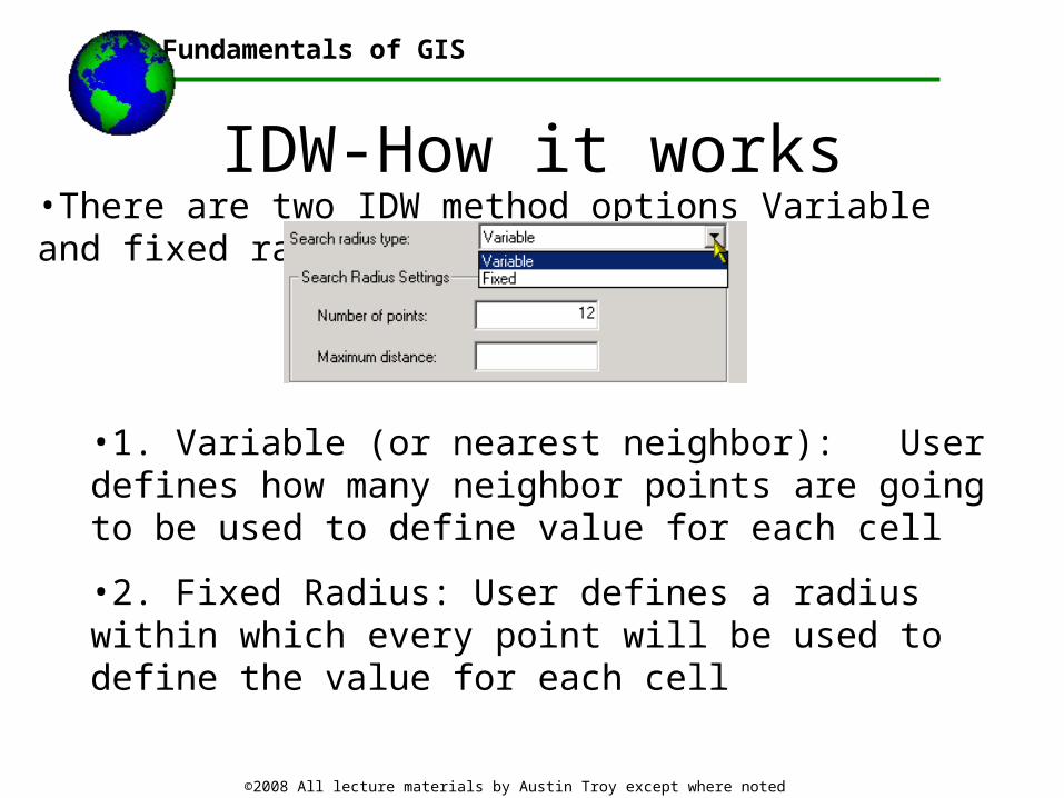
IDW-How it works•There are two IDW method options Variable and fixed radius:

•1. Variable (or nearest neighbor): User defines how many neighbor points are going to be used to define value for each cell

•2. Fixed Radius: User defines a radius within which every point will be used to define the value for each cell

Fundamentals of GIS


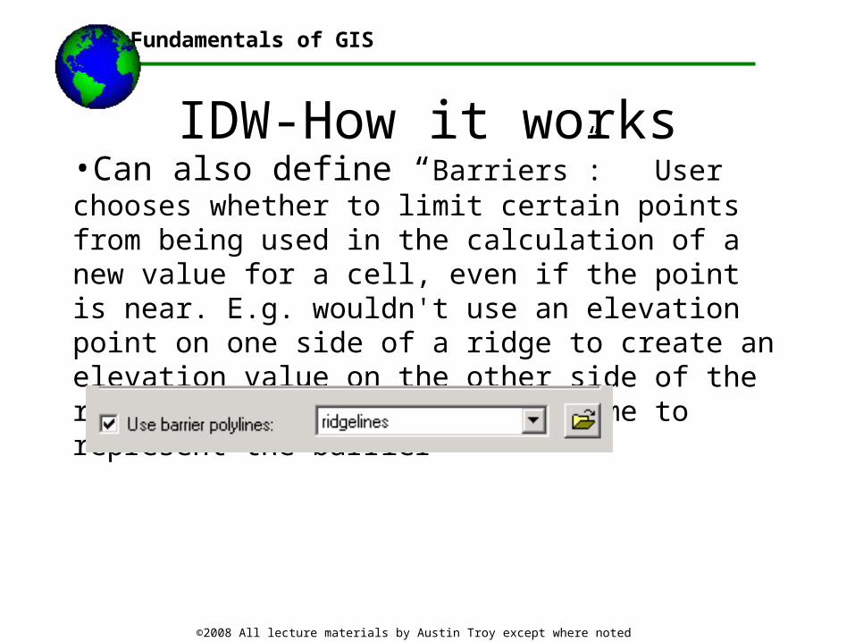
IDW-How it works•Can also define “Barriers”: User chooses whether to limit certain points from being used in the calculation of a new value for a cell, even if the point is near. E.g. wouldn't use an elevation point on one side of a ridge to create an elevation value on the other side of the ridge. User chooses a line theme to represent the barrier

Fundamentals of GIS


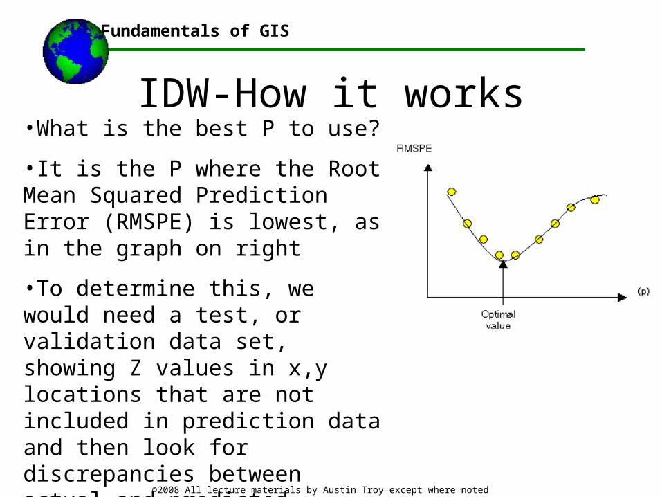
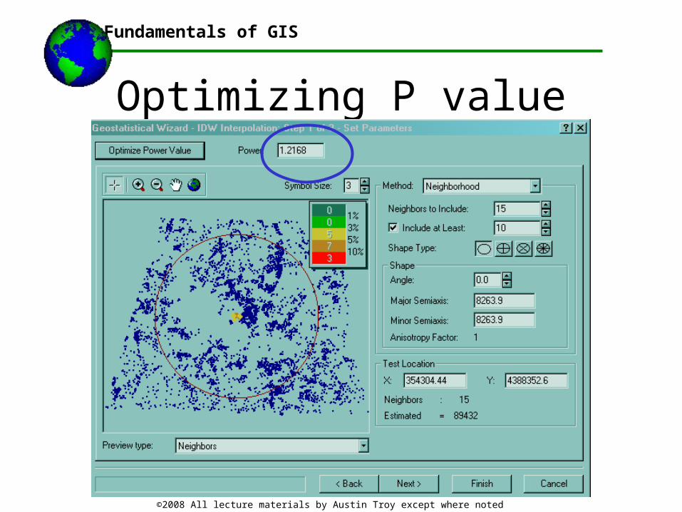
IDW-How it works•What is the best P to use?

•It is the P where the Root Mean Squared Prediction Error (RMSPE) is lowest, as in the graph on right

•To determine this, we would need a test, or validation data set, showing Z values in x,y locations that are not included in prediction data and then look for discrepancies between actual and predicted values. We keep changing the P value until we get the minimum level of error. Without this, we just guess.

Fundamentals of GIS


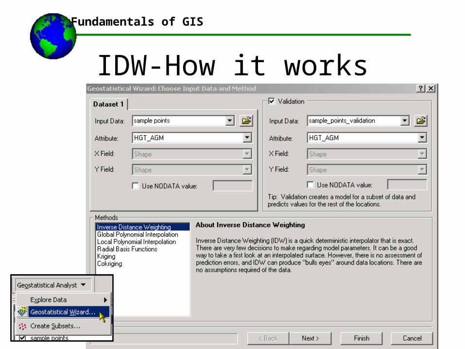
IDW-How it works•This can be done in ArcGIS using the Geostatistical Wizard

•You can look for an optimal P by testing your sample point data against a validation data set

•This validation set can be another point layer or a raster layer

•Example: we have elevation data points and we generate a DTM. We then validate our newly created DTM against an existing DTM, or against another existing elevation points data set. The computer determine what the optimum P is to minimize our error

Fundamentals of GIS


IDW-How it works

Fundamentals of GIS


Optimizing P value

Fundamentals of GIS


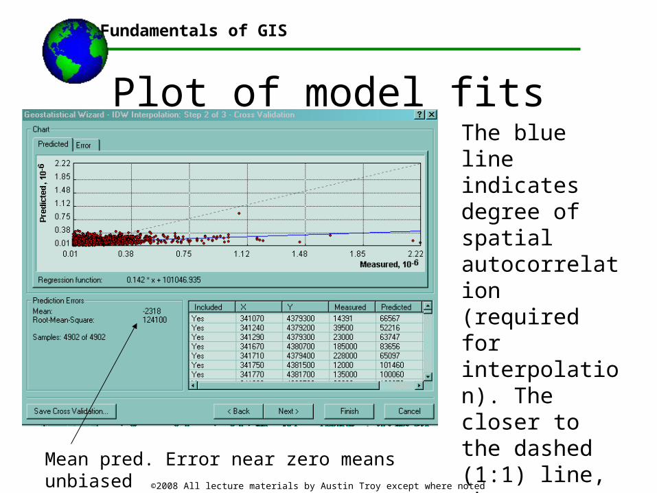
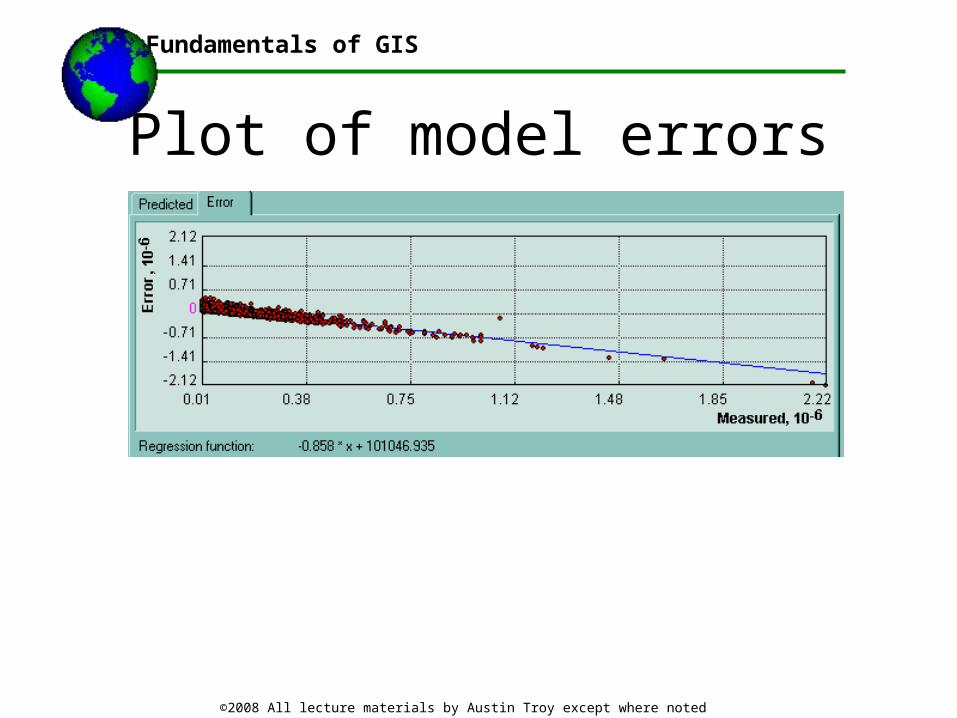
Plot of model fitsThe blue line indicates degree of spatial autocorrelation (required for interpolation). The closer to the dashed (1:1) line, the more perfectly autocorrelated.

Where horizontal, indicates data independence Mean pred. Error near zero means unbiased

Fundamentals of GIS


Plot of model errors

Fundamentals of GIS


Spline Method•Another option for interpolation method

•This fits a curve through the sample data assign values to other locations based on their location on the curve

•Thin plate splines create a surface that passes through sample points with the least possible change in slope at all points, that is with a minimum curvature surface.

•Uses piece-wise functions fitted to a small number of data points, but joins are continuous, hence can modify one part of curve without having to recompute whole

•Overall function is continuous with continuous first and second derivatives.

Fundamentals of GIS


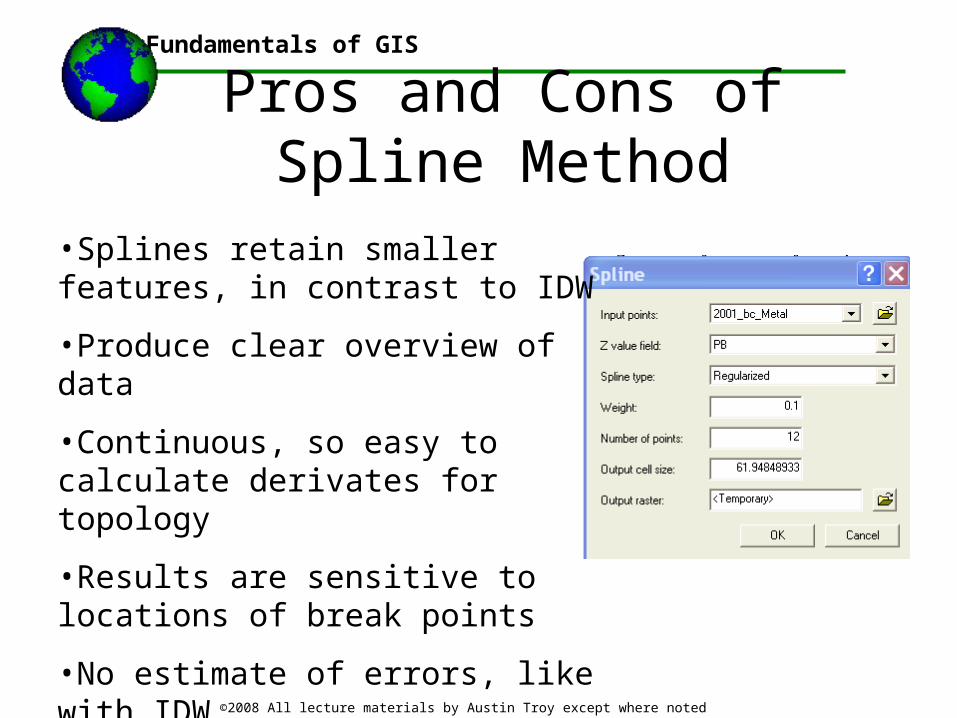
Spline Method•SPLINE has two types: regularized and tension

•Tension results in a rougher surface that more closely adheres to abrupt changes in sample points

•Regularized results in a smoother surface that smoothes out abruptly changing values somewhat

Fundamentals of GIS


Spline Method•Weight: this controls the tautness of the curves. High weight value with the Regularized Type, will result in an increasingly smooth output surface. Under the Tension Type, increases in the Weight will cause the surface to become stiffer, eventually conforming closely to the input points.

•Number of points around a cell that will be used to fit a polynomial function to a curve

Fundamentals of GIS


Pros and Cons of Spline Method

•Splines retain smaller features, in contrast to IDW

•Produce clear overview of data

•Continuous, so easy to calculate derivates for topology

•Results are sensitive to locations of break points

•No estimate of errors, like with IDW

•Can often result in over-smooth surfaces

Fundamentals of GIS


Kriging Method•Like IDW interpolation, Kriging forms weights from surrounding measured values to predict values at unmeasured locations. As with IDW interpolation, the closest measured values usually have the most influence. However, the kriging weights for the surrounding measured points are more sophisticated than those of IDW. IDW uses a simple algorithm based on distance, but kriging weights come from a semivariogram that was developed by looking at the spatial structure of the data. To create a continuous surface or map of the phenomenon, predictions are made for locations in the study area based on the semivariogram and the spatial arrangement of measured values that are nearby.

--from ESRI Help

Fundamentals of GIS

Kriging Method• In other words, kriging substitutes the arbitrarily chosen

p from IDW with a probabilistically-based weighting function that models the spatial dependence of the data.

• The structure of the spatial dependence is quantified in the semi-variogram

• Semivariograms measure the strength of statistical correlation as a function of distance; they quantify spatial autocorrelation

• Kriging associates some probability with each prediction, hence it provides not just a surface, but some measure of the accuracy of that surface

• Kriging equations are estimated through least squares


Fundamentals of GIS


Kriging Method•Kriging has both a deterministic, stochastic and random error component Z(s) = μ(s) + ε’(s)+ ε’’(s), where

μ(s) = deterministic component

ε’(s)= stochastic but spatially dependent component

ε’’(s)= spatially independent residual error

•Assumes spatial variation in variable is too irregular to be modeled by simple smooth function, better with stochastic surface

•Interpolation parameters (e.g. weights) are chosen to optimize fn

Fundamentals of GIS


Kriging Method

• Hence, foundation of Kriging is notion of spatial autocorrelation, or tendency of values of entities closer in space to be related.

• This is a violation of classical statistical models, which assumes that observations are independent.

• Autocorrelation can be assessed using a semivariogram, which plots the difference in pair values (variance) against their distances.

Fundamentals of GIS


Semivariance

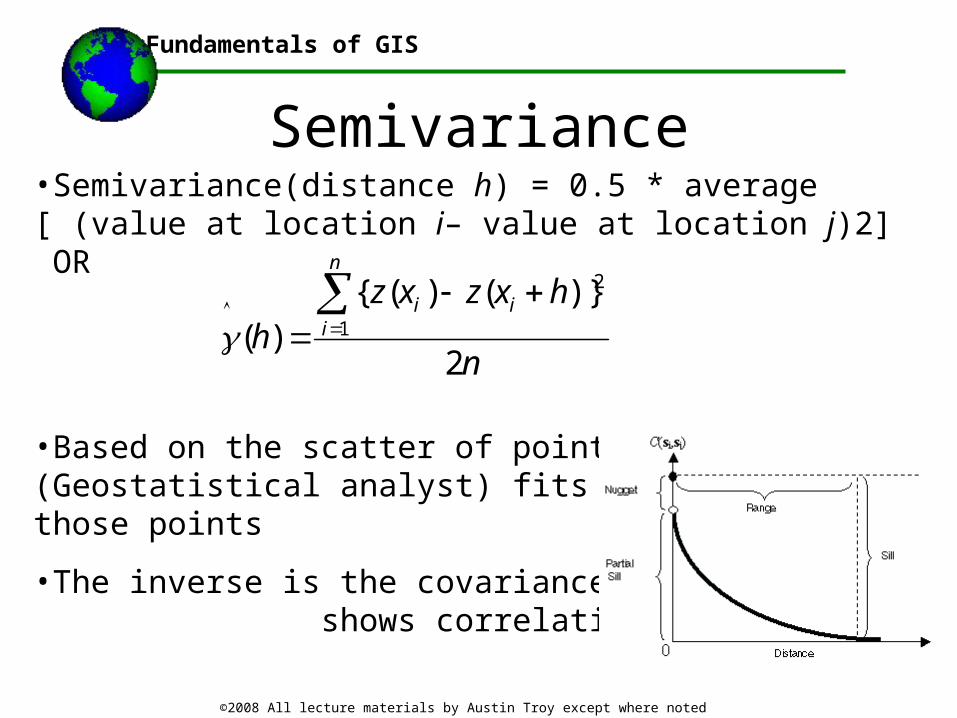
n

hxzxzh

n

iii

2

)}()({)( 1

2

•Semivariance(distance h) = 0.5 * average [ (value at location i– value at location j)2] OR

•Based on the scatter of points, the computer (Geostatistical analyst) fits a curve through those points

•The inverse is the covariance matrix whichshows correlation over space

Fundamentals of GIS

Variogram


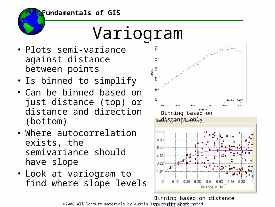
• Plots semi-variance against distance between points

• Is binned to simplify• Can be binned based on just

distance (top) or distance and direction (bottom)

• Where autocorrelation exists, the semivariance should have slope

• Look at variogram to find where slope levels

Binning based on distance only

Binning based on distance and direction

Fundamentals of GIS

Variogram


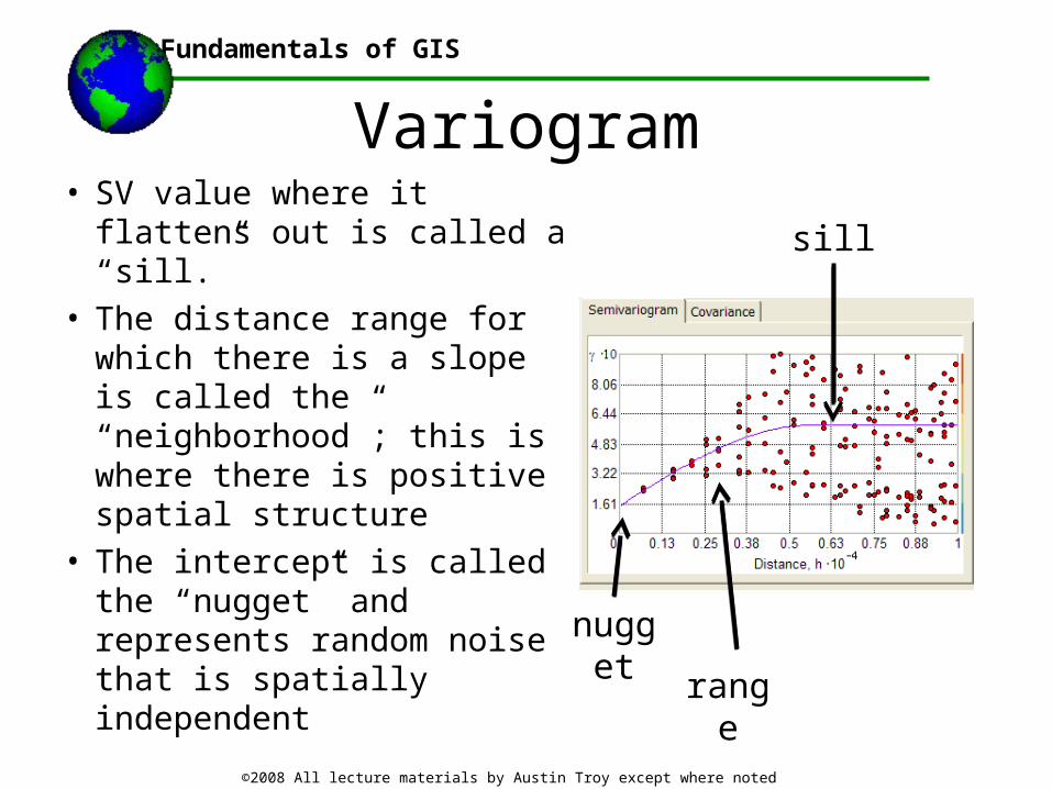
• SV value where it flattens out is called a “sill.”

• The distance range for which there is a slope is called the “neighborhood”; this is where there is positive spatial structure

• The intercept is called the “nugget” and represents random noise that is spatially independent

sill

range

nugget

Fundamentals of GIS

Steps

• Variogram cloud; can use bins to make cloud plot of all points or box plot of points

• Empirical variogram: choose bins and lags

• Model variogram: fit function through empirical variogram– Functional forms?

Fundamentals of GIS

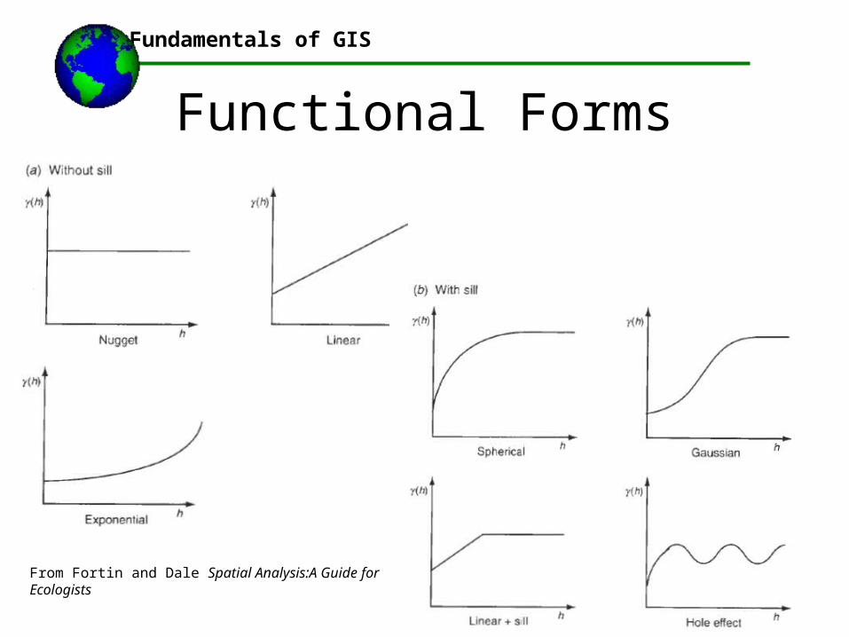
Functional Forms

From Fortin and Dale Spatial Analysis:A Guide for Ecologists

Fundamentals of GIS


Kriging Method•We can then use a scatter plot of predicted versus actual values to see the extent to which our model actually predicts the values

•If the blue line and the points lie along the 1:1 line this indicates that the kriging model predicts the data well

Fundamentals of GIS


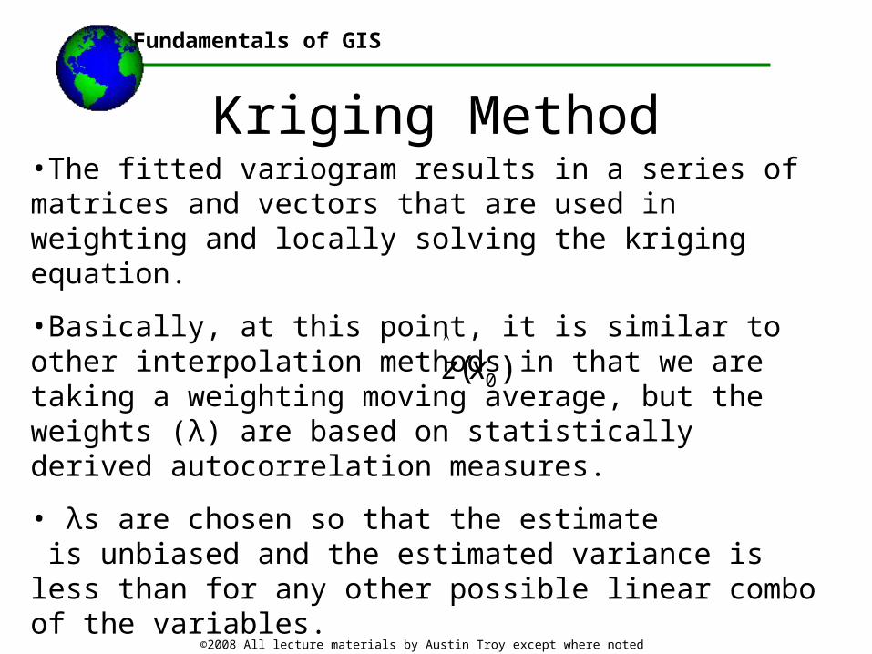
Kriging Method•The fitted variogram results in a series of matrices and vectors that are used in weighting and locally solving the kriging equation.

•Basically, at this point, it is similar to other interpolation methods in that we are taking a weighting moving average, but the weights (λ) are based on statistically derived autocorrelation measures.

• λs are chosen so that the estimate is unbiased and the estimated variance is less than for any other possible linear combo of the variables.

)( 0xz

Fundamentals of GIS


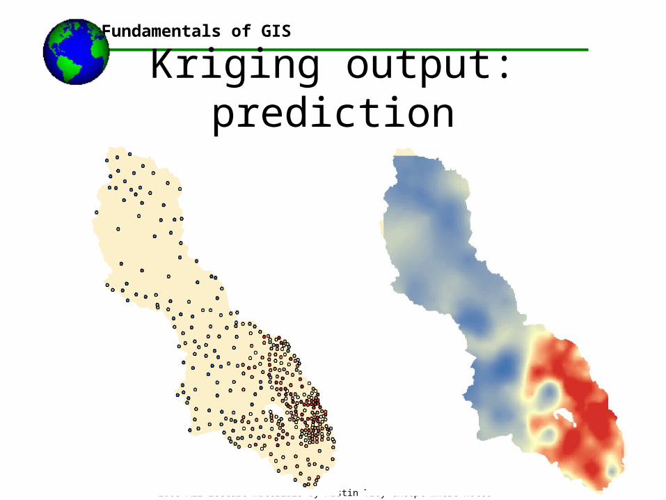
Kriging Method•Produces four types of prediction maps:

•Prediction Map: Predicted values

•Probability Map: Probability that value over x

•Prediction Standard Error Map: fit of model

•Quantile maps: Probability that value over certain quantile

Fundamentals of GIS

Kriging output: prediction


Fundamentals of GIS


Kriging: Ordinary vs. Universal

•Known as Kriging in the presence of universal trends.

•Universal kriging is used where there is an underlying trend beyond the simple spatial autocorrelation

•Generally this trend occurs at a different scale

•Trend may be fn of some geographic feature that occurs on one part of the map

Fundamentals of GIS


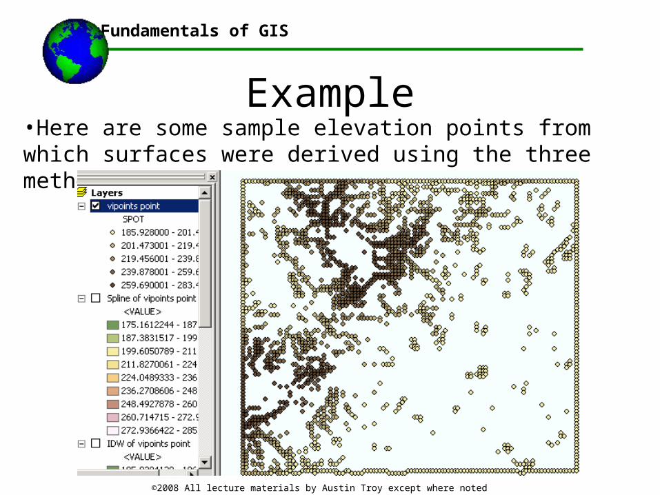
Example•Here are some sample elevation points from which surfaces were derived using the three methods

Fundamentals of GIS


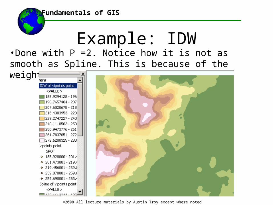
Example: IDW•Done with P =2. Notice how it is not as smooth as Spline. This is because of the weighting function introduced through P

Fundamentals of GIS


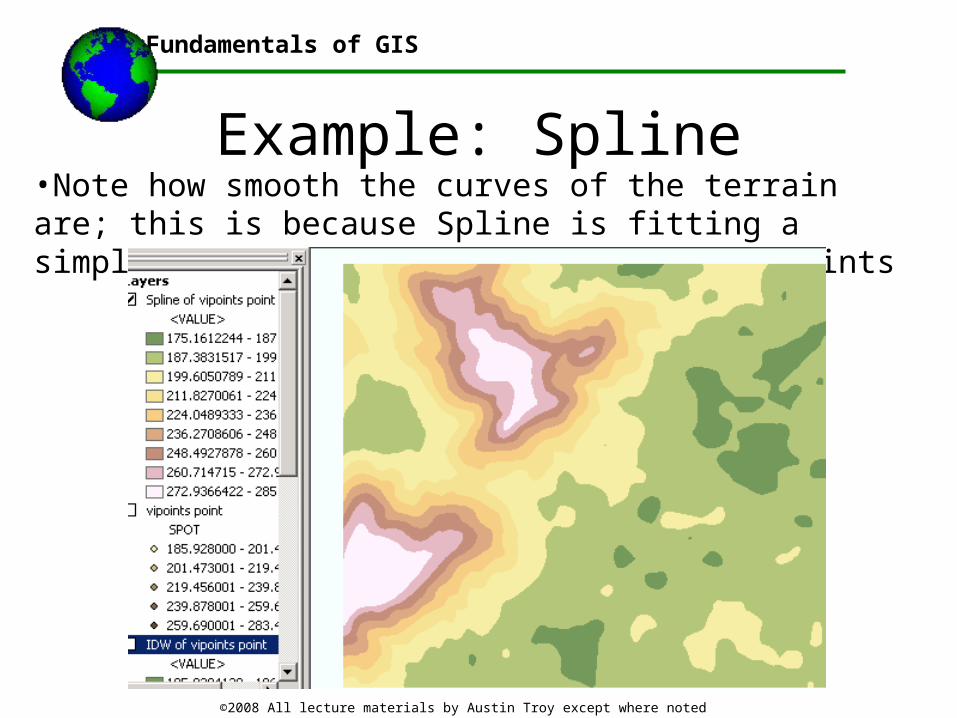
Example: Spline•Note how smooth the curves of the terrain are; this is because Spline is fitting a simply polynomial equation through the points

Fundamentals of GIS


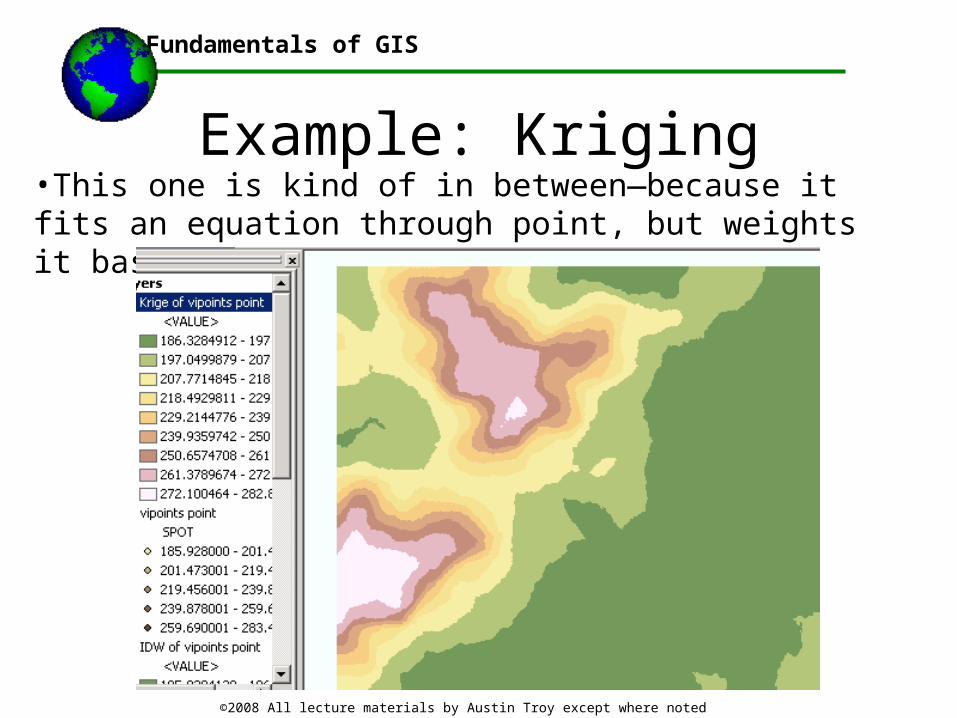
Example: Kriging•This one is kind of in between—because it fits an equation through point, but weights it based on probabilities

Fundamentals of GIS


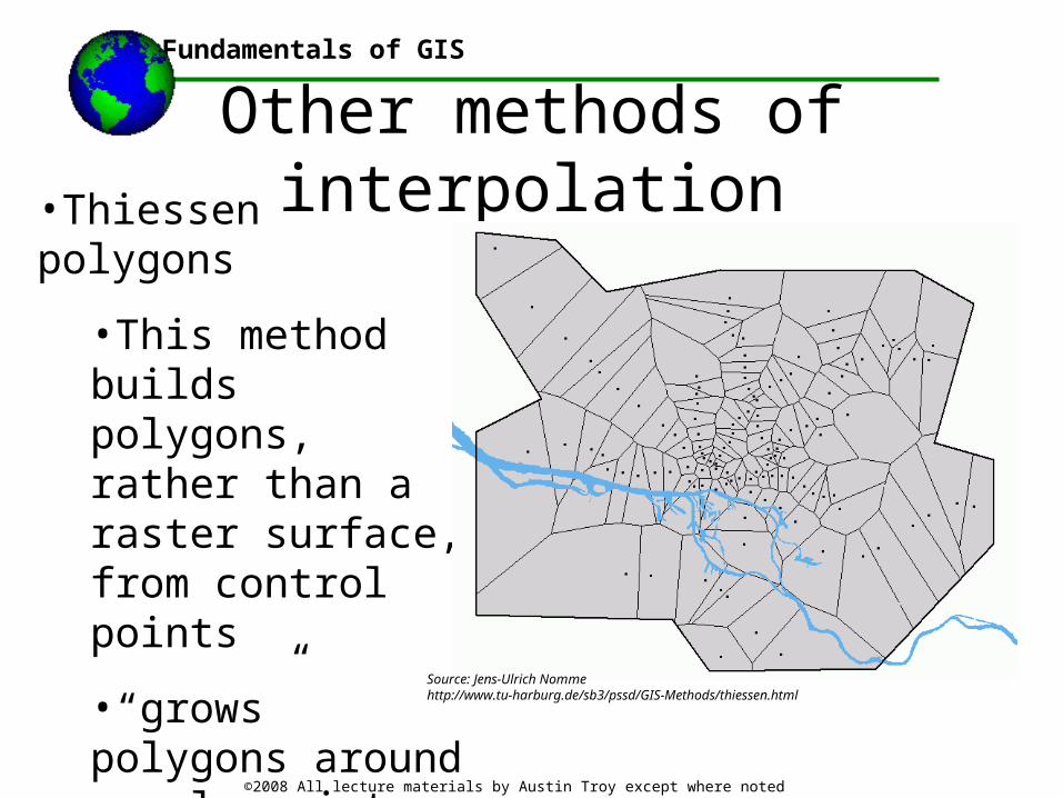
Other methods of interpolation•Thiessen polygons

•This method builds polygons, rather than a raster surface, from control points

•“grows” polygons around sample points that are supposed to represent areas of homogeneity

Source: Jens-Ulrich Nomme http://www.tu-harburg.de/sb3/pssd/GIS-Methods/thiessen.html

fundamentals of gis ©2008 all lecture materials by austin troy except where noted lecture 10:...

Documents