fundamentals of digital communications and data...
TRANSCRIPT
Fundamentals of Digital
Communications and Data Transmission
29th October 2008
Abdullah Al-Meshal

Overview
• Introduction
– Communication systems
– Digital communication system
– Importance of Digital transmission
• Basic Concepts in Signals
– Sampling
– Quantization
– Coding
Digital Communication Abdullah Al-Meshal
What is Communication?
• Communication is transferring data reliably
from one point to another
– Data could be: voice, video, codes etc…
• It is important to receive the sameinformation that was sent from thetransmitter.
• Communication system
– A system that allows transfer of informationrealiably
Digital Communication Abdullah Al-Meshal
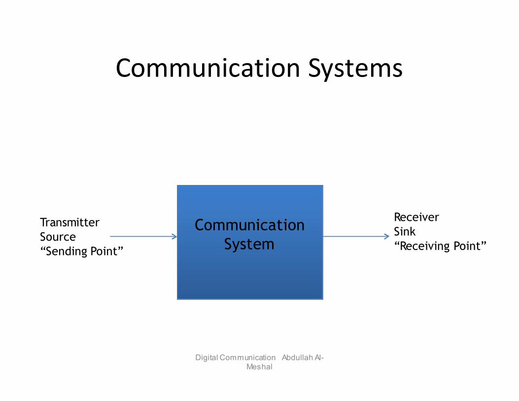
Communication Systems
Digital Communication Abdullah Al-Meshal
Communication
System
Transmitter
Source
“Sending Point”
Receiver
Sink
“Receiving Point”
Digital Communication Abdullah Al-Meshal
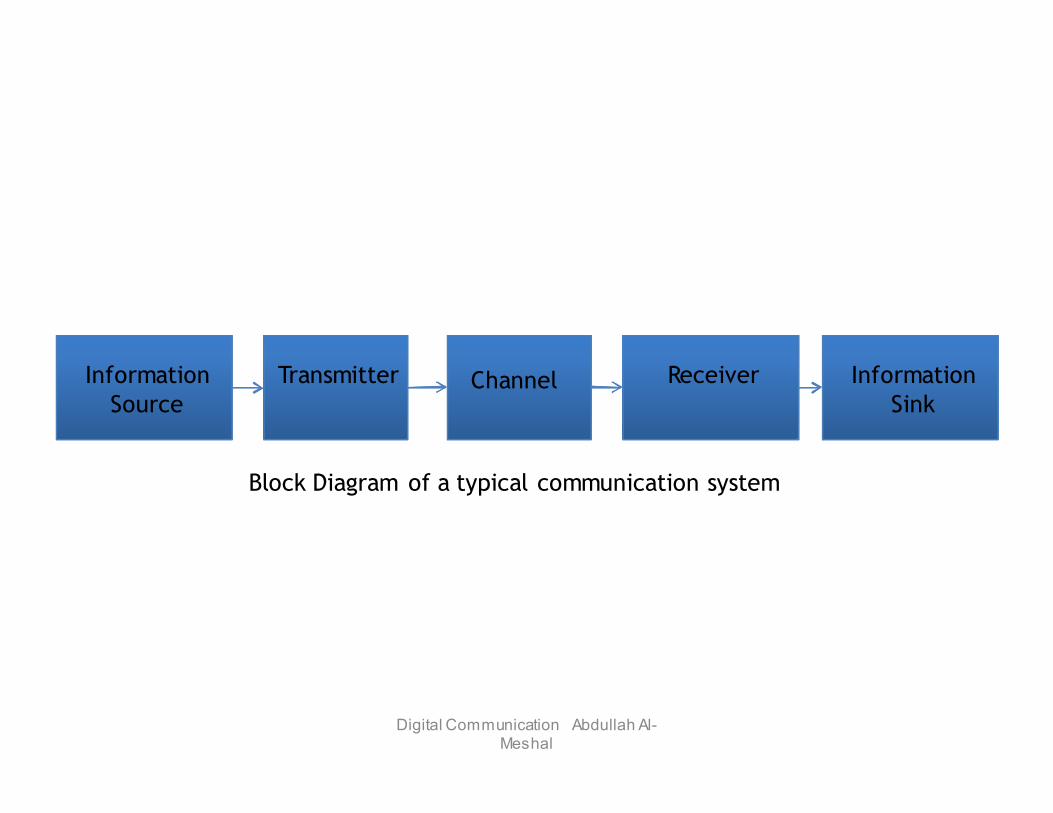
Information
Source
Transmitter Channel Receiver Information
Sink
Block Diagram of a typical communication system
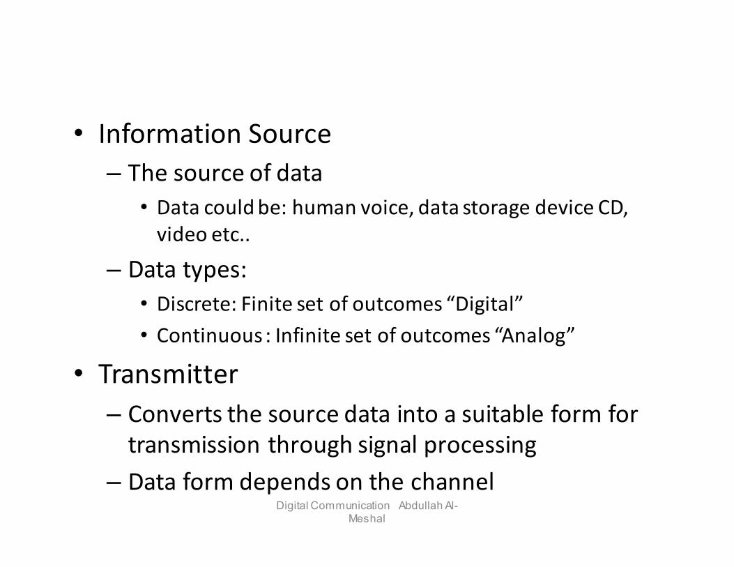
• Information Source
– The source of data
• Data could be: human voice, data storage device CD,
video etc..
– Data types:
• Discrete: Finite set of outcomes “Digital”
• Continuous : Infinite set of outcomes “Analog”
• Transmitter
– Converts the source data into a suitable form for
transmission through signal processing
– Data form depends on the channelDigital Communication Abdullah Al-
Meshal
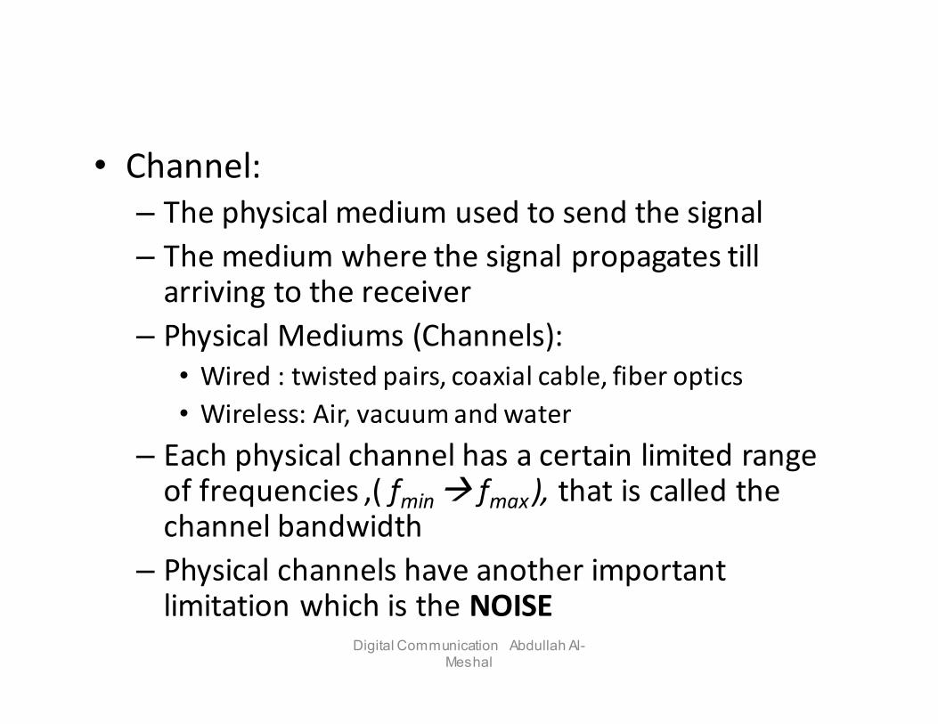
• Channel:
– The physical medium used to send the signal
– The medium where the signal propagates till arriving to the receiver
– Physical Mediums (Channels):
• Wired : twisted pairs, coaxial cable, fiber optics
• Wireless: Air, vacuum and water
– Each physical channel has a certain limited range of frequencies ,( fmin � fmax ), that is called the channel bandwidth
– Physical channels have another important limitation which is the NOISE
Digital Communication Abdullah Al-Meshal
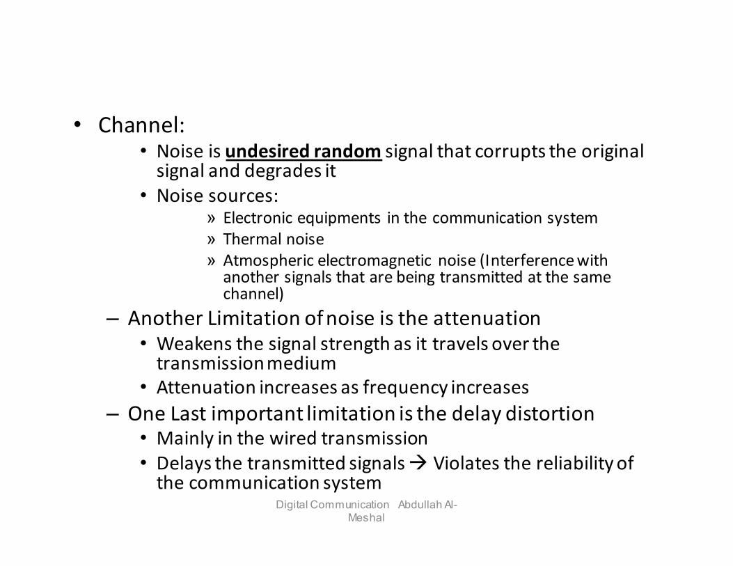
• Channel:• Noise is undesired random signal that corrupts the original
signal and degrades it
• Noise sources:» Electronic equipments in the communication system
» Thermal noise
» Atmospheric electromagnetic noise (Interference with another signals that are being transmitted at the same channel)
– Another Limitation of noise is the attenuation
• Weakens the signal strength as it travels over the transmission medium
• Attenuation increases as frequency increases
– One Last important limitation is the delay distortion• Mainly in the wired transmission
• Delays the transmitted signals � Violates the reliability of the communication system
Digital Communication Abdullah Al-Meshal
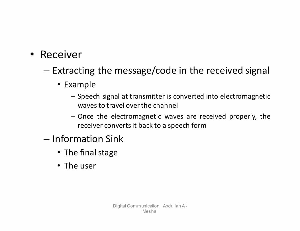
• Receiver
– Extracting the message/code in the received signal
• Example
– Speech signal at transmitter is converted into electromagnetic
waves to travel over the channel
– Once the electromagnetic waves are received properly, the
receiver converts it back to a speech form
– Information Sink
• The final stage
• The user
Digital Communication Abdullah Al-Meshal
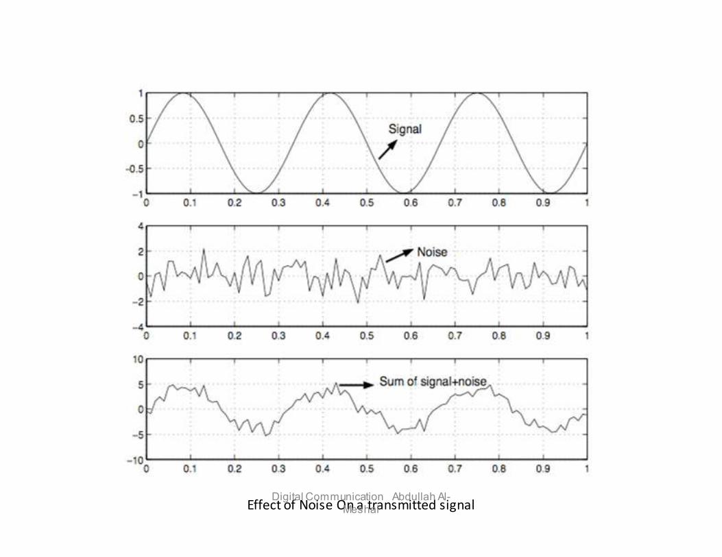
Effect of Noise On a transmitted signalDigital Communication Abdullah Al-
Meshal
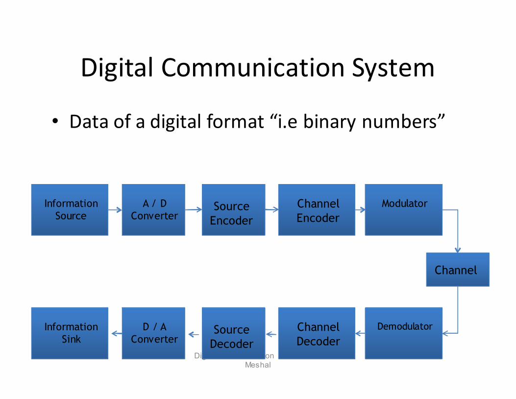
Digital Communication System
• Data of a digital format “i.e binary numbers”
Digital Communication Abdullah Al-Meshal
Information
Source
A / D
ConverterSource
Encoder
Channel
Encoder
Modulator
Information
Sink
D / A
ConverterSource
Decoder
Channel
Decoder
Demodulator
Channel
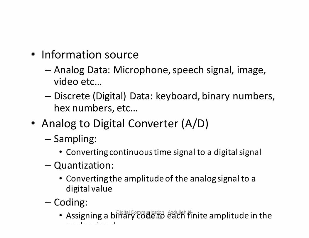
• Information source
– Analog Data: Microphone, speech signal, image, video etc…
– Discrete (Digital) Data: keyboard, binary numbers, hex numbers, etc…
• Analog to Digital Converter (A/D)
– Sampling:
• Converting continuous time signal to a digital signal
– Quantization:
• Converting the amplitude of the analog signal to a digital value
– Coding:
• Assigning a binary code to each finite amplitude in the analog signal
Digital Communication Abdullah Al-Meshal
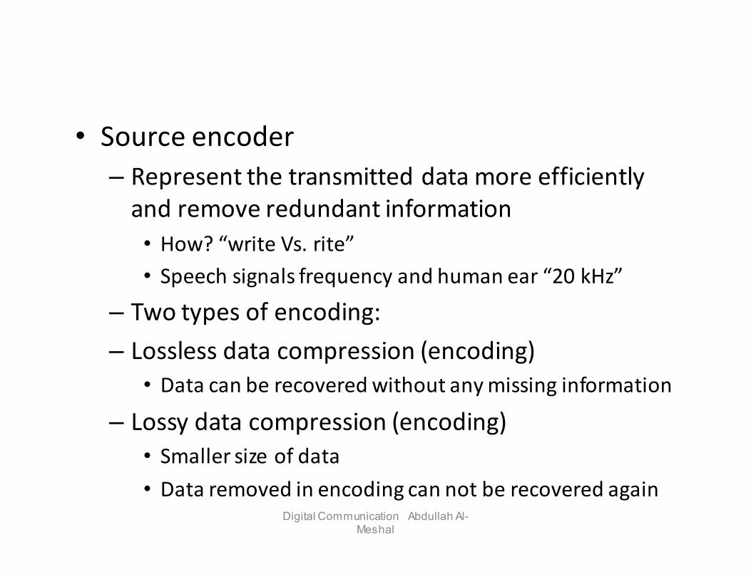
• Source encoder
– Represent the transmitted data more efficiently
and remove redundant information
• How? “write Vs. rite”
• Speech signals frequency and human ear “20 kHz”
– Two types of encoding:
– Lossless data compression (encoding)
• Data can be recovered without any missing information
– Lossy data compression (encoding)
• Smaller size of data
• Data removed in encoding can not be recovered againDigital Communication Abdullah Al-
Meshal
• Channel encoder:
– To control the noise and to detect and correct the
errors that can occur in the transmitted data due
the noise.
• Modulator:
– Represent the data in a form to make it
compatible with the channel
• Carrier signal “high frequency signal”
• Demodulator:
– Removes the carrier signal and reverse the
process of the ModulatorDigital Communication Abdullah Al-
Meshal
• Channel decoder:
– Detects and corrects the errors in the signal
gained from the channel
• Source decoder:
– Decompresses the data into it’s original format.
• Digital to Analog Converter:
– Reverses the operation of the A/D
– Needs techniques and knowledge about sampling,
quantization, and coding methods.
• Information Sink
– The UserDigital Communication Abdullah Al-
Meshal
Why should we use digital communication?
• Ease of regeneration– Pulses “ 0 , 1”
– Easy to use repeaters
• Noise immunity– Better noise handling when using repeaters that repeats
the original signal
– Easy to differentiate between the values “either 0 or 1”
• Ease of Transmission
– Less errors
– Faster !
– Better productivity
Digital Communication Abdullah Al-Meshal
Why should we use digital communication?
• Ease of multiplexing
– Transmitting several signals simultaneously
• Use of modern technology
– Less cost !
• Ease of encryption
– Security and privacy guarantee
– Handles most of the encryption techniques
Digital Communication Abdullah Al-Meshal
Disadvantage !
• The major disadvantage of digital transmission
is that it requires a greater transmission
bandwidth or channel bandwidth to
communicate the same information in digital
format as compared to analog format.
• Another disadvantage of digital transmission is
that digital detection requires system
synchronization, whereas analog signals
generally have no such requirement.
Digital Communication Abdullah Al-Meshal

Chapter 2: Analog to Digital
Conversion (A/D)
Abdullah Al-Meshal

Digital Communication System
Information
Source
A / D
ConverterSource
Encoder
Channel
Encoder
Modulator
Information
Sink
D / A
ConverterSource
Decoder
Channel
Decoder
Demodulator
Channel
2.1 Basic Concepts in Signals
• A/D is the process of converting an analog
signal to digital signal, in order to transmit it
through a digital communication system.
• Electric Signals can be represented either in
Time domain or frequency domain.
– Time domain i.e
– We can get the value of that signal at any time (t)
by substituting in the v(t) equation.
v(t) = 2sin(2π1000t + 45)
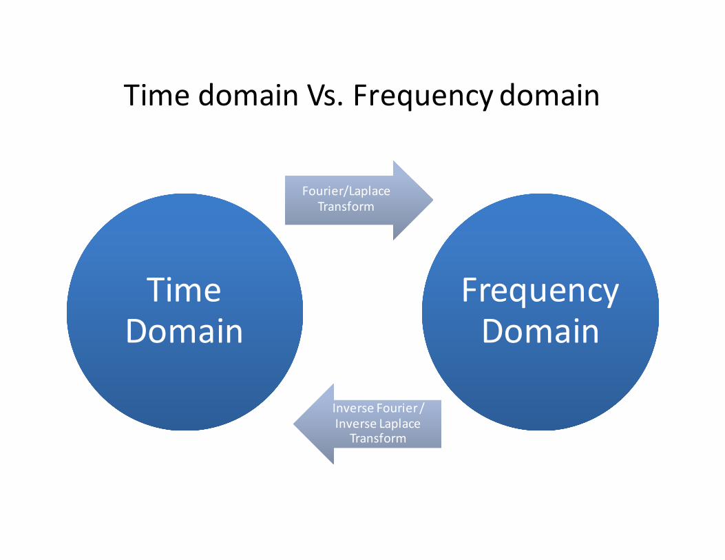
Time domain Vs. Frequency domain
Time Domain
Time Domain
Fourier/Laplace
Transform
Fourier/Laplace
Transform
Frequency Domain
Frequency Domain
Inverse Fourier /
Inverse Laplace Transform
Inverse Fourier /
Inverse Laplace Transform
Time domain Vs. Frequency domain
• Consider taking two types of images of a person:
• Passport image
• X-Ray image
• Two different domains, spatial domain “passport image”
and “X-Ray domain”.
• Doctors are taking the image in the X-Ray domain to
extract more information about the patient.
• Different domains helps fetching and gaining knowledge
about an object.
– An Object : Electric signal, human body, etc…
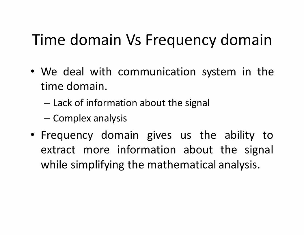
Time domain Vs Frequency domain
• We deal with communication system in the
time domain.
– Lack of information about the signal
– Complex analysis
• Frequency domain gives us the ability to
extract more information about the signal
while simplifying the mathematical analysis.
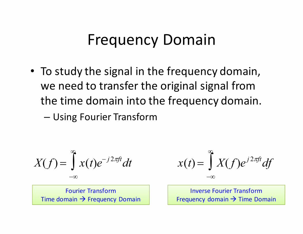
Frequency Domain
• To study the signal in the frequency domain,
we need to transfer the original signal from
the time domain into the frequency domain.
– Using Fourier Transform
X( f ) = x(t)e− j 2πft
dt−∞
∞
∫ x(t) = X( f )ej 2πft
df−∞
∞
∫
Fourier Transform
Time domain � Frequency Domain
Inverse Fourier Transform
Frequency domain � Time Domain
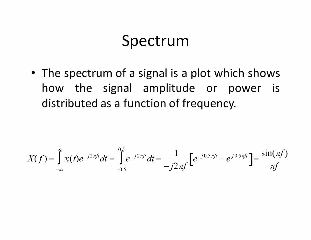
Spectrum
• The spectrum of a signal is a plot which shows
how the signal amplitude or power is
distributed as a function of frequency.
X( f ) = x(t)e− j2πftdt = e− j 2πftdt =1
− j2πfe− j 0.5πft − e j 0.5πft[ ]
−0.5
0.5
∫−∞
∞
∫ =sin(πf )πf
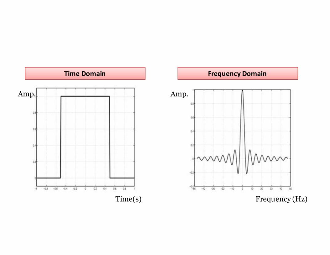
Time Domain Frequency Domain
Amp. Amp.
Time(s) Frequency (Hz)
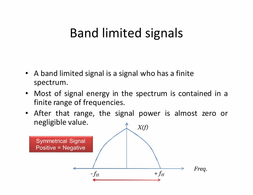
Band limited signals
• A band limited signal is a signal who has a finite spectrum.
• Most of signal energy in the spectrum is contained in afinite range of frequencies.
• After that range, the signal power is almost zero ornegligible value.
X(f)
+ fH- fHFreq.
Symmetrical SignalPositive = Negative
Converting an Analog Signal to a Discrete
Signal (A/D)
• Can be done through three basic steps:
1- Sampling
2- Quantization
3- Coding
Sampling
• Process of converting the continuous time
signal to a discrete time signal.
• Sampling is done by taking “Samples” at
specific times spaced regularly.
– V(t) is an analog signal
– V(nTs) is the sampled signal
• Ts = positive real number that represent the spacing of
the sampling time
• n = sample number integer
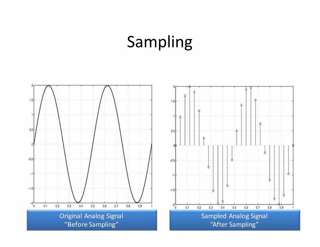
Sampling
Original Analog Signal
“Before Sampling”
Sampled Analog Signal
“After Sampling”
Sampling
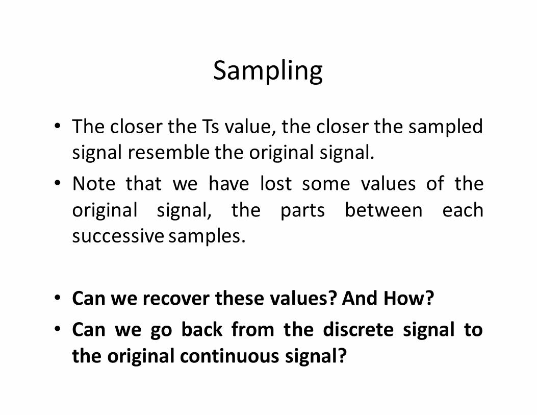
• The closer the Ts value, the closer the sampled
signal resemble the original signal.
• Note that we have lost some values of the
original signal, the parts between each
successive samples.
• Can we recover these values? And How?
• Can we go back from the discrete signal to
the original continuous signal?
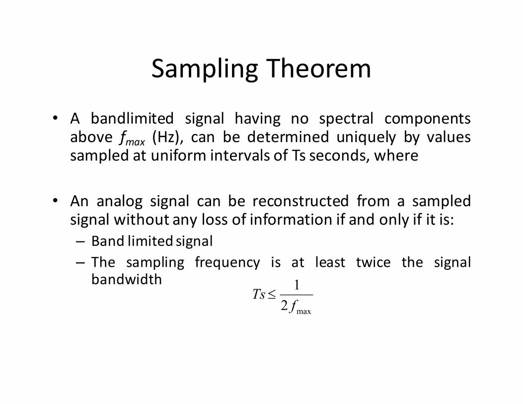
Sampling Theorem
• A bandlimited signal having no spectral componentsabove fmax (Hz), can be determined uniquely by valuessampled at uniform intervals of Ts seconds, where
• An analog signal can be reconstructed from a sampledsignal without any loss of information if and only if it is:
– Band limited signal
– The sampling frequency is at least twice the signalbandwidth
Ts ≤1
2 fmax
Quantization
• Quantization is a process of approximating a
continuous range of values, very large set of
possible discrete values, by a relatively small
range of values, small set of discrete values.
• Continuous range � infinte set of values
• Discrete range � finite set of values
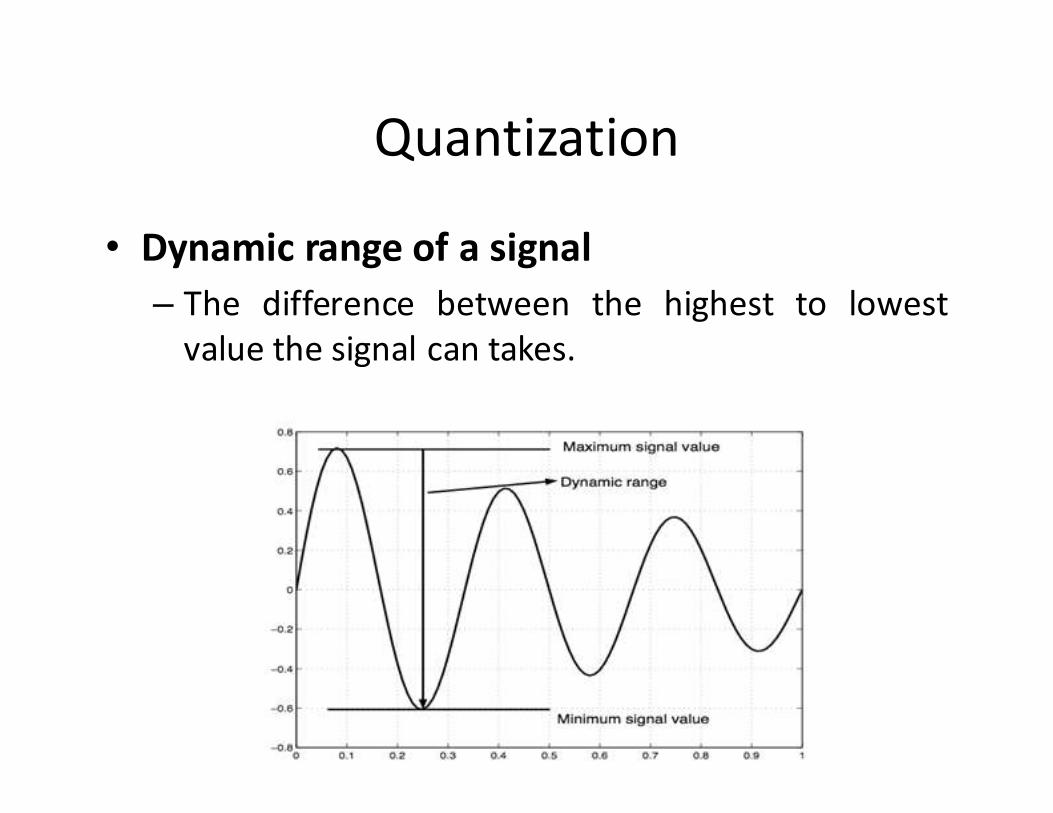
Quantization
• Dynamic range of a signal
– The difference between the highest to lowest
value the signal can takes.
Quantization
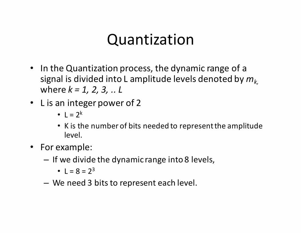
• In the Quantization process, the dynamic range of a signal is divided into L amplitude levels denoted by mk,
where k = 1, 2, 3, .. L
• L is an integer power of 2
• L = 2k
• K is the number of bits needed to represent the amplitude level.
• For example:
– If we divide the dynamic range into 8 levels,
• L = 8 = 23
– We need 3 bits to represent each level.
Quantization
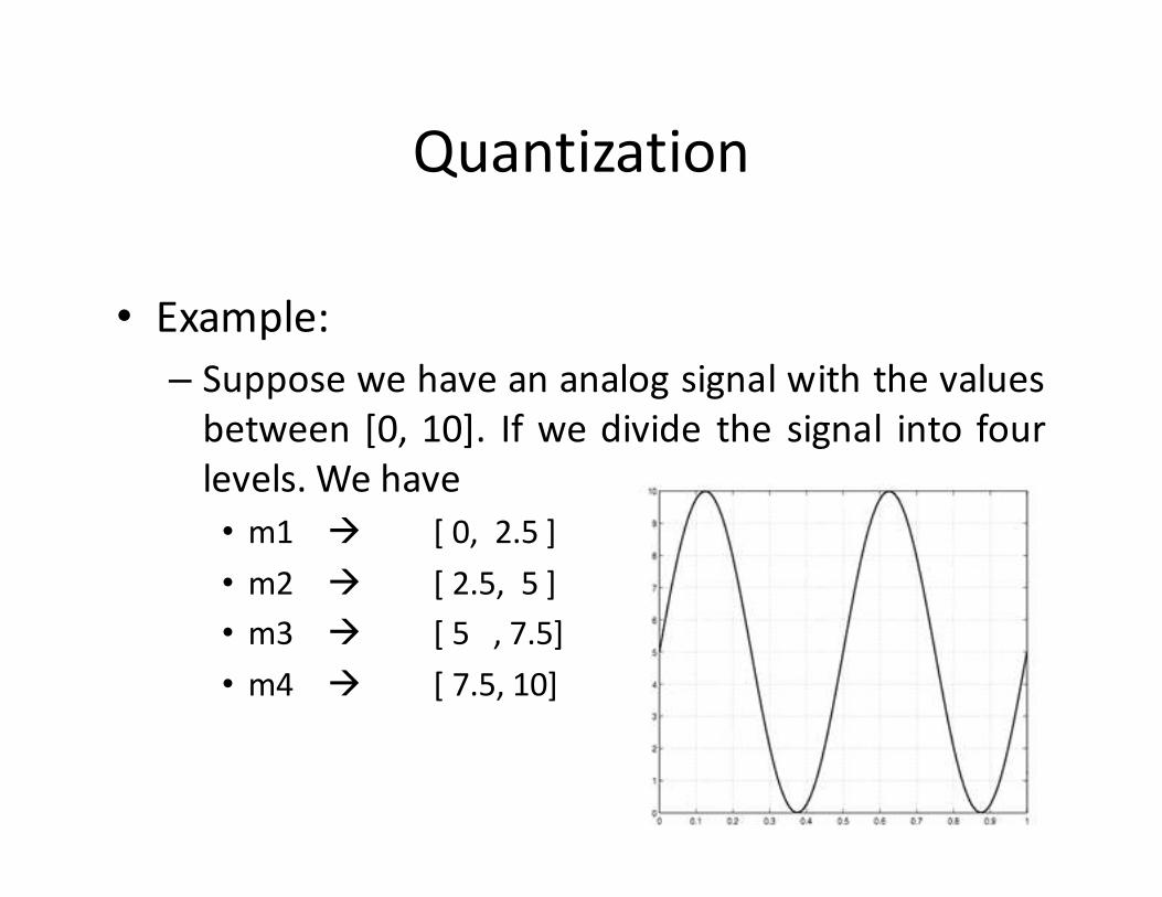
• Example:
– Suppose we have an analog signal with the values
between [0, 10]. If we divide the signal into four
levels. We have
• m1 � [ 0, 2.5 ]
• m2 � [ 2.5, 5 ]
• m3 � [ 5 , 7.5]
• m4 � [ 7.5, 10]
Quantization
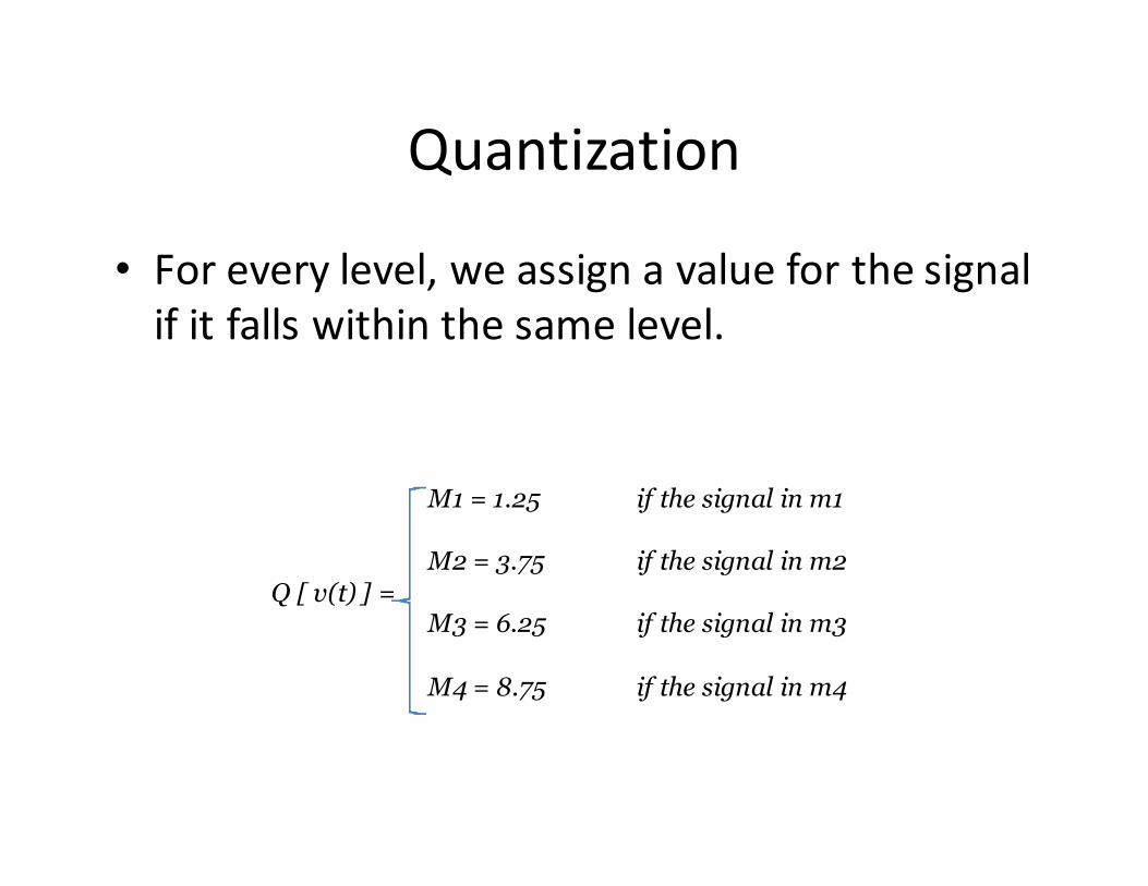
• For every level, we assign a value for the signal
if it falls within the same level.
M1 = 1.25 if the signal in m1
M2 = 3.75 if the signal in m2
Q [ v(t) ] = M3 = 6.25 if the signal in m3
M4 = 8.75 if the signal in m4
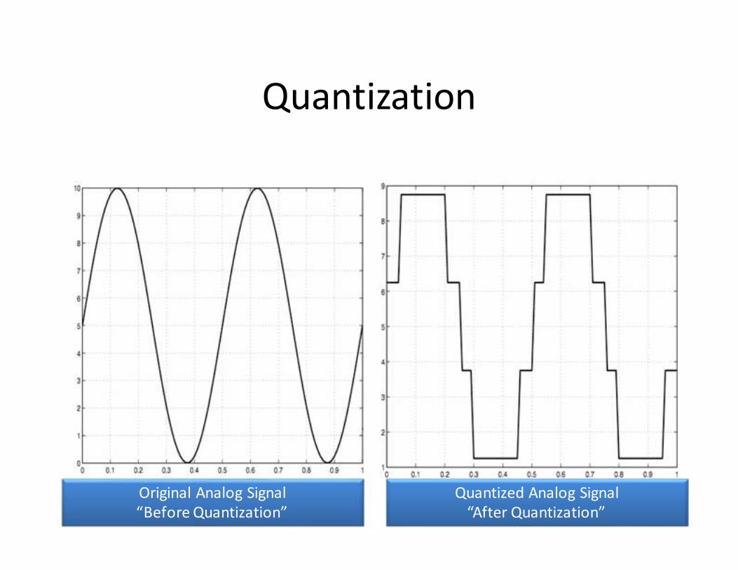
Quantization
Original Analog Signal
“Before Quantization”
Quantized Analog Signal
“After Quantization”
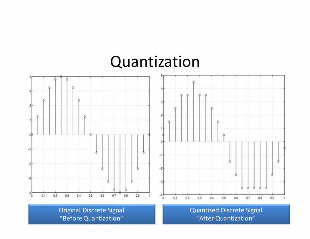
Quantization
Original Discrete Signal
“Before Quantization”
Quantized Discrete Signal
“After Quantization”

Quantization
• The more quantization levels we take the
smaller the error between the original and
quantized signal.
• Quantization step
• The smaller the Δ the smaller the error.
∆ =Dynamic Range
No. of Quantization levels=Smax
− Smin
L
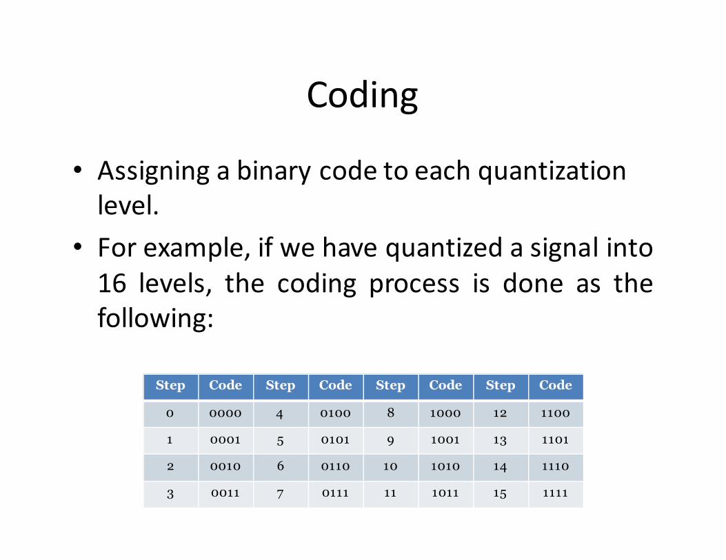
Coding
• Assigning a binary code to each quantization
level.
• For example, if we have quantized a signal into
16 levels, the coding process is done as the
following:
Step Code Step Code Step Code Step Code
0 0000 4 0100 8 1000 12 1100
1 0001 5 0101 9 1001 13 1101
2 0010 6 0110 10 1010 14 1110
3 0011 7 0111 11 1011 15 1111
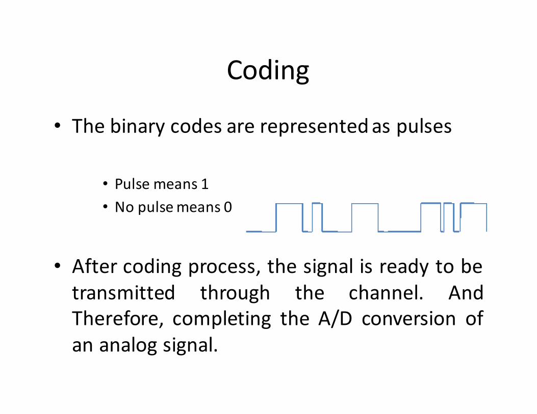
Coding
• The binary codes are represented as pulses
• Pulse means 1
• No pulse means 0
• After coding process, the signal is ready to be
transmitted through the channel. And
Therefore, completing the A/D conversion of
an analog signal.
Chapter 3: Source Coding
12th November 2008
Abdullah Al-Meshal
3.1 Measure of Information
• What is the definition of “Information” ?• News, text data, images, videos, sound etc..
• In Information Theory– Information is linked with the element of surprise or
uncertainty
– In terms of probability
– Information • The more probable some event to occur the less information
related to its occurrence.
• The less probable some event to occur the more information we get when it occurs.

Example1:
• The rush hour in Kuwait is between 7.00 am –8.00 am
– A person leaving his home to work at 7.30 willNOT be surprised about the traffic jam � almostno information is gained here
– A person leaving his home to work at 7.30 will BE surprised if THERE IS NO traffic jam:
– He will start asking people / family / friends
– Unusual experience
– Gaining more information
Example 2
• The weather temperature in Kuwait at summerseason is usually above 30o
• It is known that from the historical data of theweather, the chance that it rains in summer isvery rare chance.– A person who lives in Kuwait will not be surprised by
this fact about the weather
– A person who lived in Kuwait will BE SURPRISED if itrains during summer, therefore asking about thephenomena. Therefore gaining more knowledge“information”
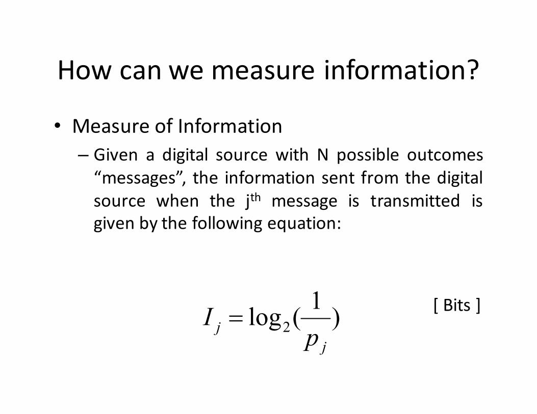
How can we measure information?
• Measure of Information
– Given a digital source with N possible outcomes
“messages”, the information sent from the digital
source when the jth message is transmitted is
given by the following equation:
[ Bits ] I j = log2(
1
p j
)
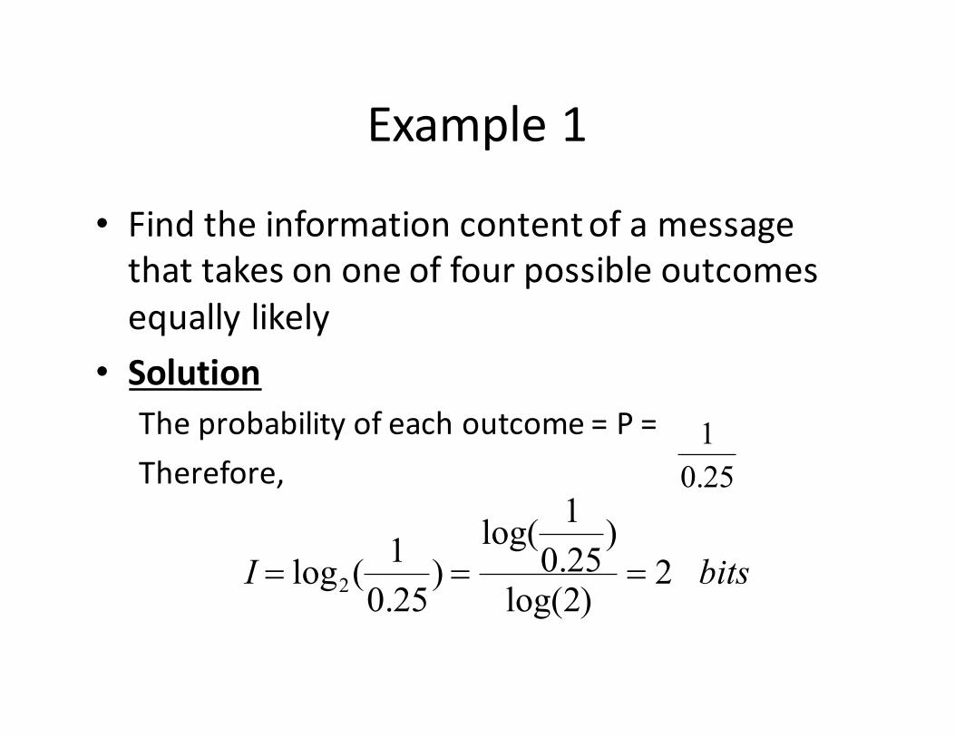
Example 1
• Find the information content of a message
that takes on one of four possible outcomes
equally likely
• Solution
The probability of each outcome = P =
Therefore,
1
0.25
I = log2(1
0.25) =
log(1
0.25)
log(2)= 2 bits
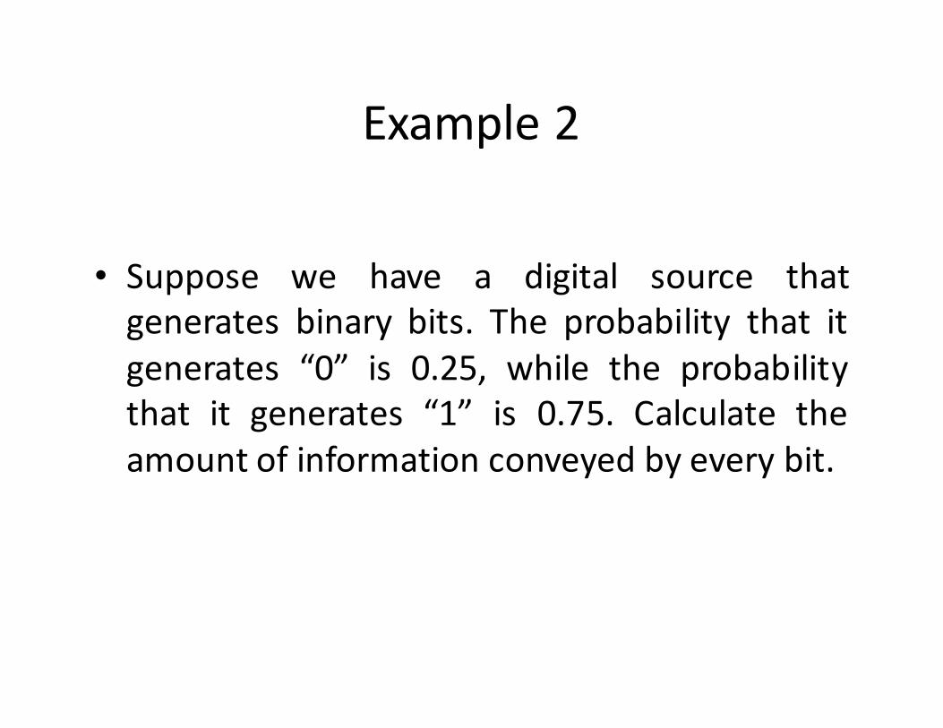
Example 2
• Suppose we have a digital source that
generates binary bits. The probability that it
generates “0” is 0.25, while the probability
that it generates “1” is 0.75. Calculate the
amount of information conveyed by every bit.
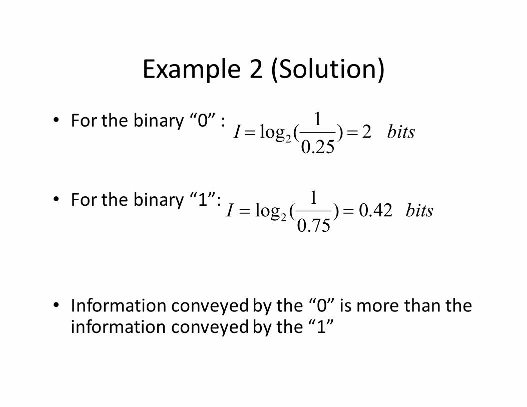
Example 2 (Solution)
• For the binary “0” :
• For the binary “1”:
• Information conveyed by the “0” is more than the information conveyed by the “1”
I = log2(1
0.25) = 2 bits
bitsI 42.0)75.0
1(log2 ==
Example 3:
• A discrete source generates a sequence of ( n )
bits. How many possible messages can we
receive from this source?
• Assuming all the messages are equally likely to
occur, how much information is conveyed by
each message?
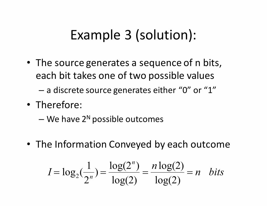
Example 3 (solution):
• The source generates a sequence of n bits,
each bit takes one of two possible values
– a discrete source generates either “0” or “1”
• Therefore:
– We have 2N possible outcomes
• The Information Conveyed by each outcome
I = log2(1
2n) =
log(2n)
log(2)=n log(2)
log(2)= n bits

3.3 Entropy
• The entropy of a discrete source S is the
average amount of information ( or
uncertainty ) associated with that source.
• m = number of possible outcomes
• Pj = probability of the jth message
H(s) = p j log2(1
p j
) [bits]j=1
m
∑
Importance of Entropy
• Entropy is considered one of the most important quantities in information theory.
• There are two types of source coding:
– Lossless coding “lossless data compression”
– Lossy coding “lossy data compression”
• Entropy is the threshold quantity that separates lossy from lossless data compression.

Example 4
• Consider an experiment of selecting a card at
random from a cards deck of 52 cards. Suppose
we’re interested in the following events:
– Getting a picture, with probability of :
– Getting a number less than 3, with probability of:
– Getting a number between 3 and 10, with a probability of:
• Calculate the Entropy of this random experiment.
52
12
8
5232
52
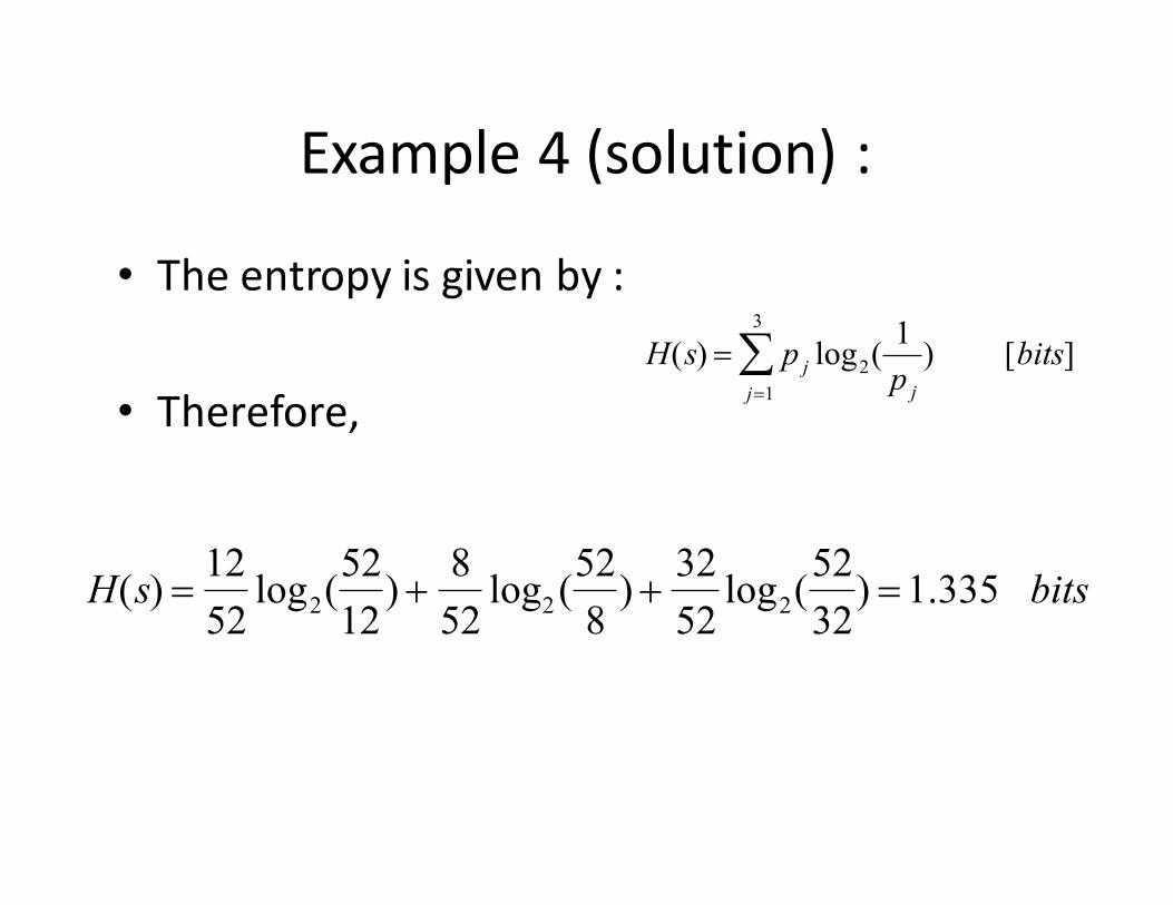
Example 4 (solution) :
• The entropy is given by :
• Therefore,
H(s) = pjlog
2(1
pj
) [bits]j=1
3
∑
H(s) =12
52log2(
52
12) +
8
52log2 (
52
8) +
32
52log2(
52
32) =1.335 bits
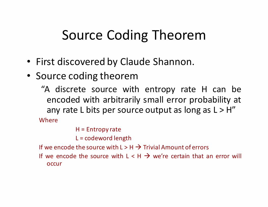
Source Coding Theorem
• First discovered by Claude Shannon.
• Source coding theorem
“A discrete source with entropy rate H can beencoded with arbitrarily small error probability atany rate L bits per source output as long as L > H”
Where
H = Entropy rate
L = codeword length
If we encode the source with L > H � Trivial Amount of errors
If we encode the source with L < H � we’re certain that an error willoccur
3.4 Lossless data compression
• Data compression
– Encoding information in a relatively smaller size than their original size
• Like ZIP files (WinZIP), RAR files (WinRAR),TAR files etc..
• Data compression:
– Lossless: the compressed data are an exact copy of the original data
– Lossy: the compressed data may be different than the original data
• Loseless data compression techniques:
– Huffman coding algorithm
– Lempel-Ziv Source coding algorithm
3.4.1 Huffman Coding Algorithm
• A digital source generates five symbols with the following probabilities:
– S , P(s)=0.27
– T, P(t)=0.25
– U, P(t)=0.22
– V,P(t)=0.17
– W,P(t)=0.09
• Use Huffman Coding algorithm to compress this source
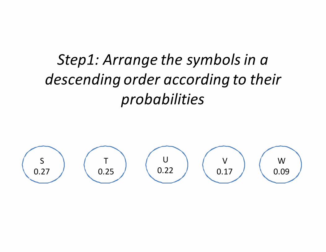
Step1: Arrange the symbols in a
descending order according to their
probabilities
S
0.27
S
0.27
T
0.25
T
0.25
U
0.22
U
0.22V
0.17
V
0.17
W
0.09
W
0.09
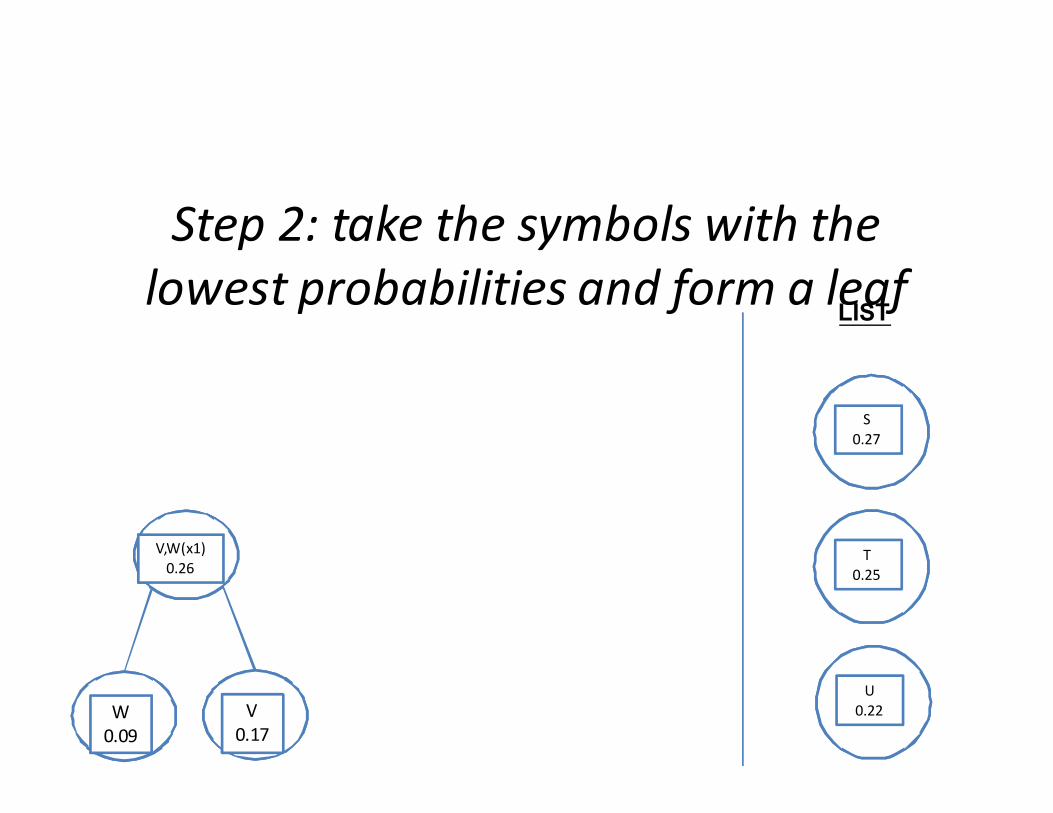
Step 2: take the symbols with the
lowest probabilities and form a leaf
V
0.17
V
0.17
U
0.22
U
0.22
LIST
T
0.25
T
0.25
S
0.27
S
0.27
W
0.09
W
0.09
V,W(x1)
0.26
V,W(x1)
0.26
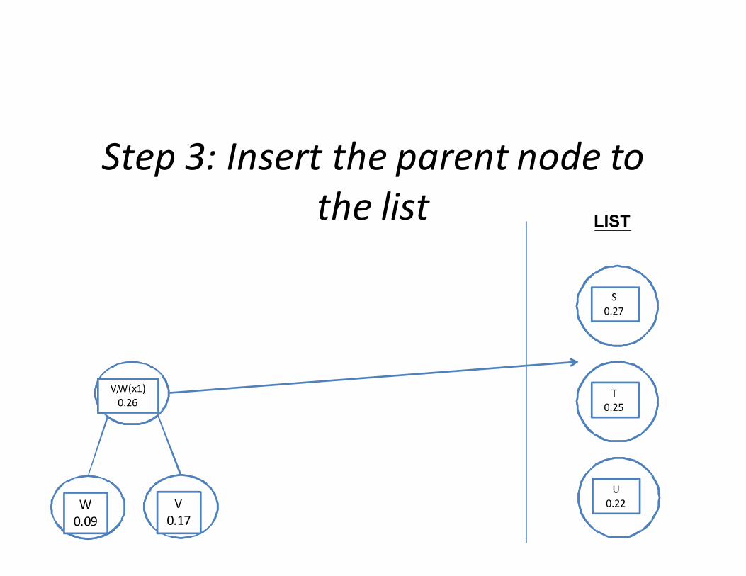
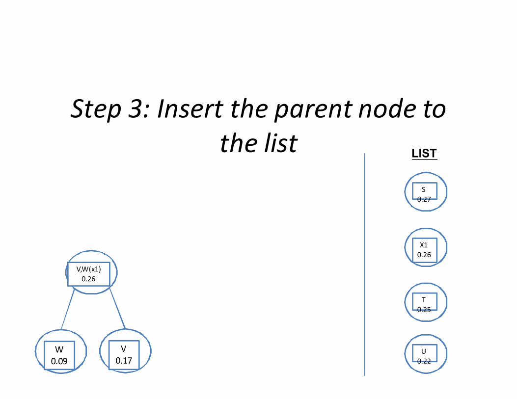
Step 3: Insert the parent node to
the list
V
0.17
V
0.17
U
0.22
U
0.22
LIST
T
0.25
T
0.25
S
0.27
S
0.27
W
0.09
W
0.09
V,W(x1)
0.26
V,W(x1)
0.26
Step 3: Insert the parent node to
the list
V
0.17
V
0.17U
0.22
U
0.22
LIST
T
0.25
T
0.25
S
0.27
S
0.27
W
0.09
W
0.09
V,W(x1)
0.26
V,W(x1)
0.26
X1
0.26
X1
0.26
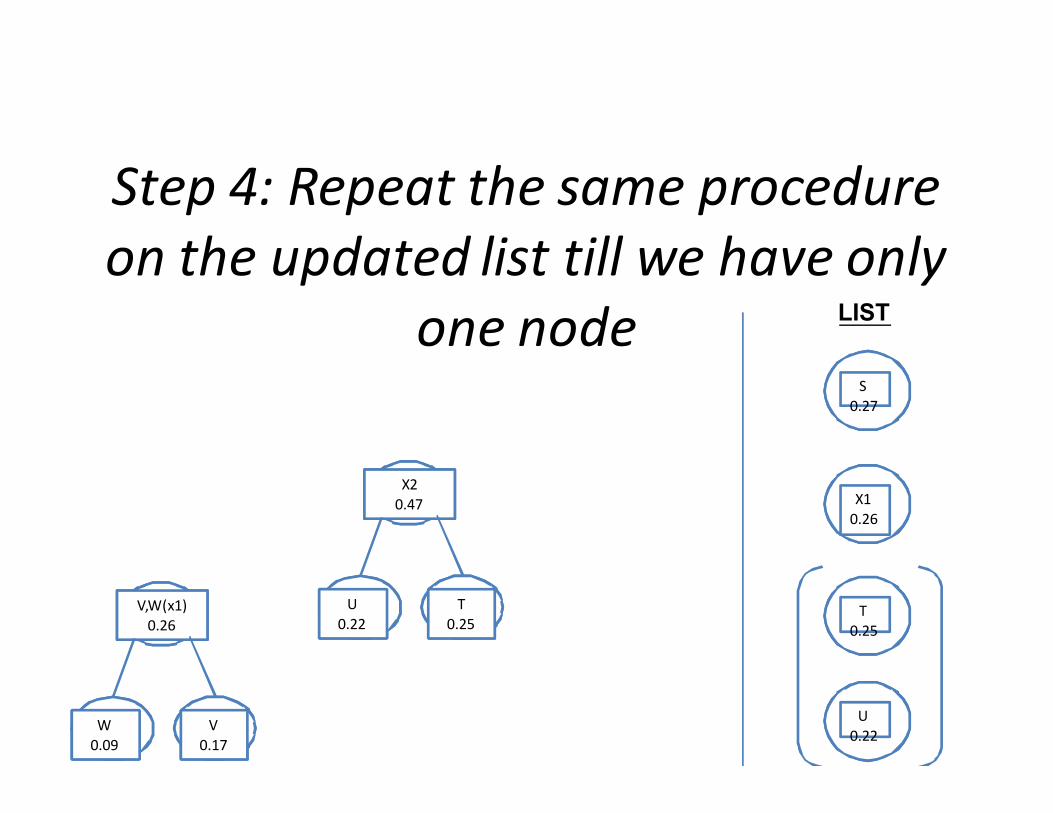
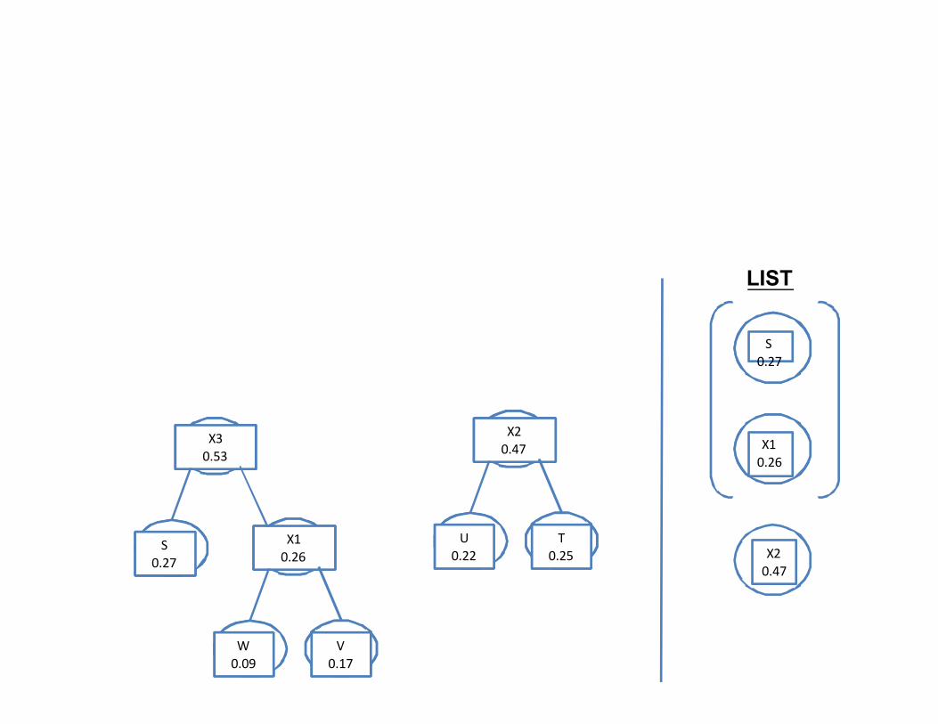
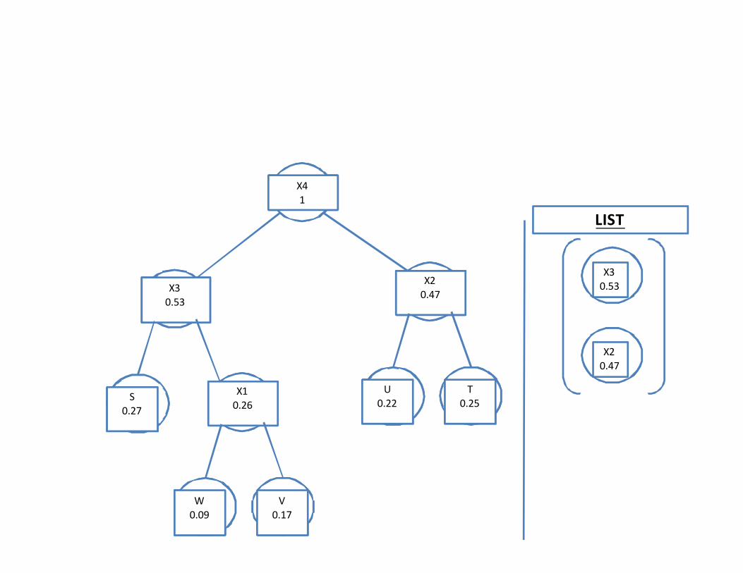
Step 4: Repeat the same procedure
on the updated list till we have only
one node
U
0.22
U
0.22
LIST
T
0.25
T
0.25
S
0.27
S
0.27
V
0.17
V
0.17
W
0.09
W
0.09
V,W(x1)
0.26
V,W(x1)
0.26
X1
0.26
X1
0.26
T
0.25
T
0.25
U
0.22
U
0.22
X2
0.47
X2
0.47
LIST
S
0.27
S
0.27
V
0.17
V
0.17
W
0.09
W
0.09
X1
0.26
X1
0.26
X1
0.26
X1
0.26
T
0.25
T
0.25
U
0.22
U
0.22
X2
0.47
X2
0.47
X2
0.47
S
0.27
S
0.27
X3
0.53
X3
0.53
LIST
X3
0.53
X3
0.53
X2
0.47
X2
0.47
V
0.17
V
0.17
W
0.09
W
0.09
X1
0.26
X1
0.26
T
0.25
T
0.25
U
0.22
U
0.22
X2
0.47
X2
0.47
S
0.27
S
0.27
X3
0.53
X3
0.53
X4
1
X4
1
V
0.17
V
0.17
W
0.09
W
0.09
X1
0.26
X1
0.26
T
0.25
T
0.25
U
0.22
U
0.22
X2
0.47
X2
0.47
S
0.27
S
0.27
X3
0.53
X3
0.53
X4
1
X4
1
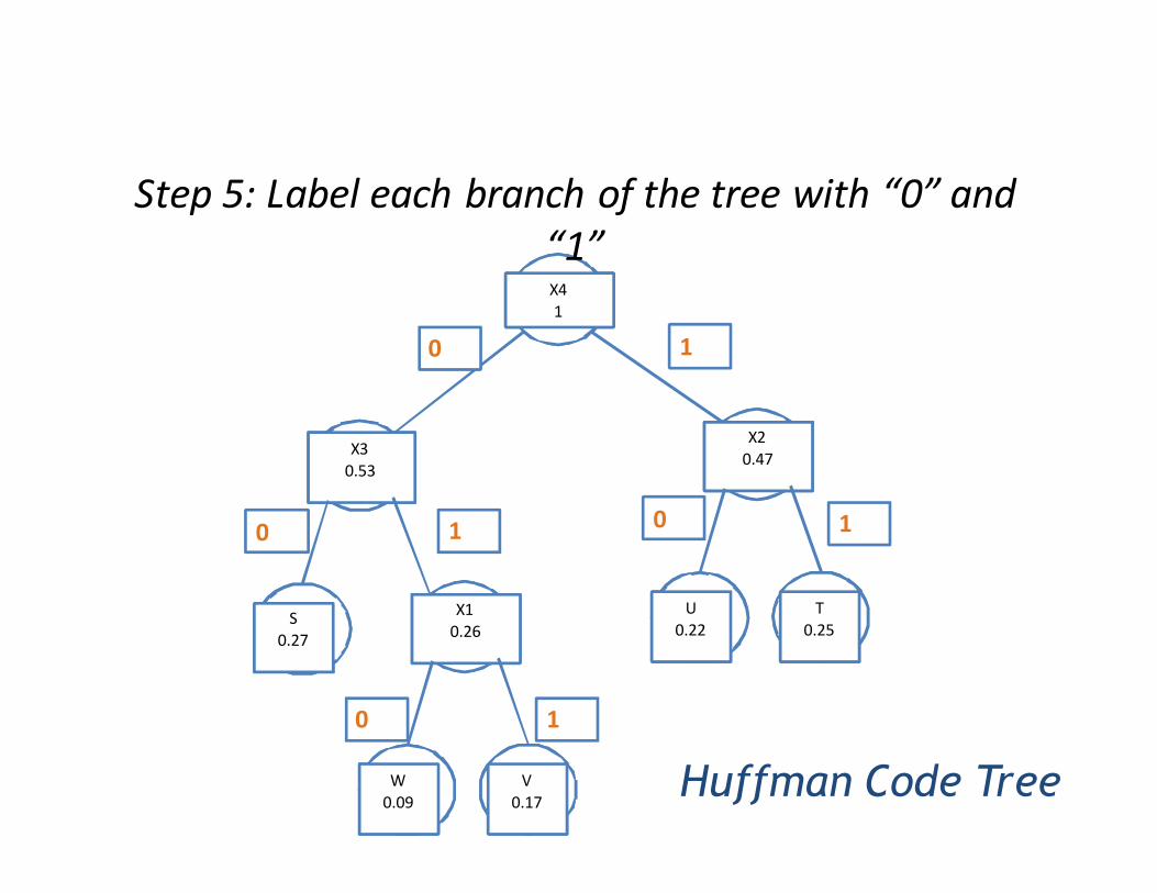
Step 5: Label each branch of the tree with “0” and
“1”
Huffman Code Tree
0
0
0
0
1
11
1

V
0.17
V
0.17
W
0.09
W
0.09
X1
0.26
X1
0.26
T
0.25
T
0.25
U
0.22
U
0.22
X2
0.47
X2
0.47
S
0.27
S
0.27
X3
0.53
X3
0.53
X4
1
X4
1
Codeword of w = 010
Huffman Code Tree
0
0
0
0
1
11
1
V
0.17
V
0.17
W
0.09
W
0.09
X1
0.26
X1
0.26
T
0.25
T
0.25
U
0.22
U
0.22
X2
0.47
X2
0.47
S
0.27
S
0.27
X3
0.53
X3
0.53
X4
1
X4
1
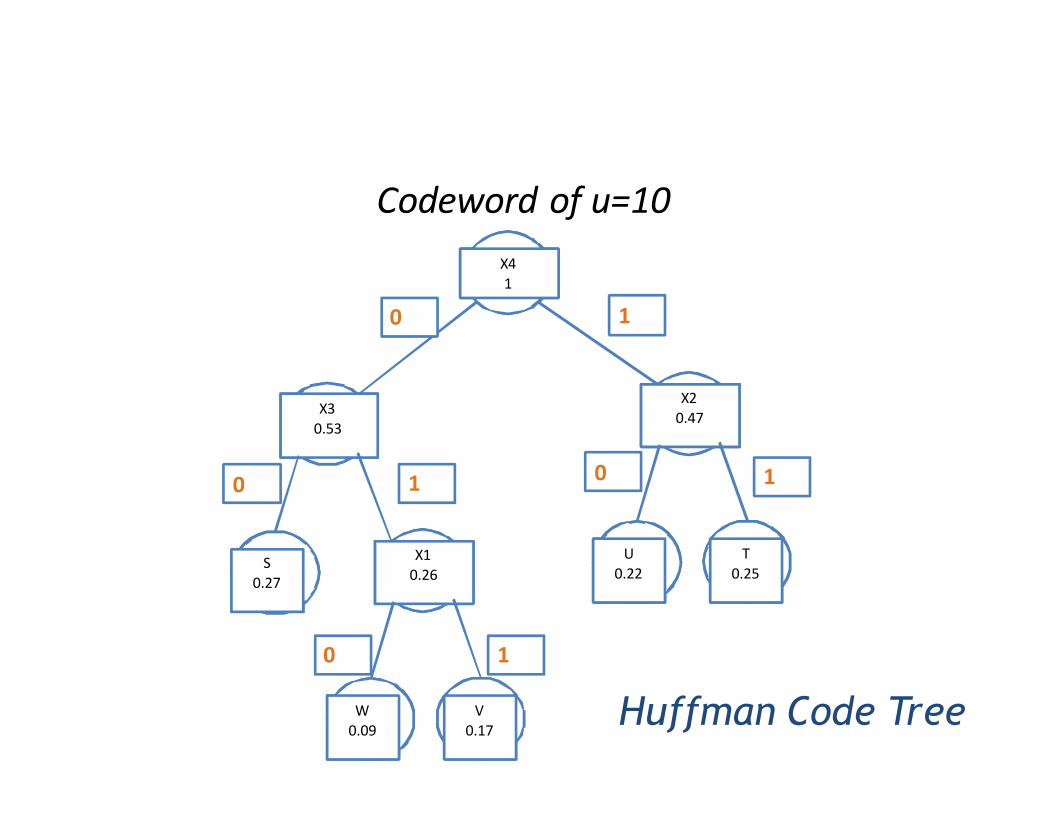
Codeword of u=10
Huffman Code Tree
0
0
0
0
1
11
1
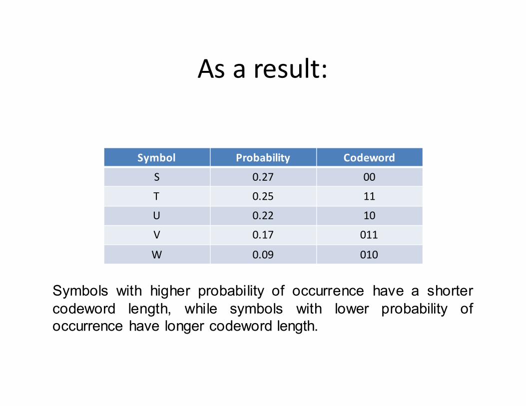
As a result:
Symbol Probability Codeword
S 0.27 00
T 0.25 11
U 0.22 10
V 0.17 011
W 0.09 010
Symbols with higher probability of occurrence have a shorter
codeword length, while symbols with lower probability of
occurrence have longer codeword length.
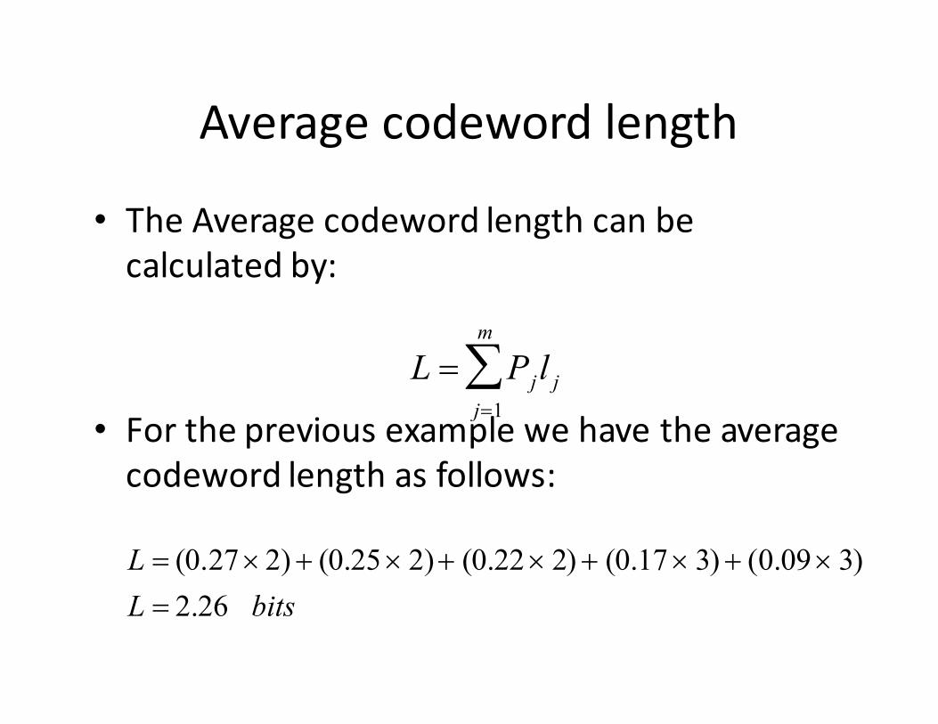
Average codeword length
• The Average codeword length can be
calculated by:
• For the previous example we have the average
codeword length as follows:
L = Pjlj
j=1
m
∑
L = (0.27×2) + (0.25× 2)+ (0.22× 2) + (0.17× 3) + (0.09× 3)
L = 2.26 bits
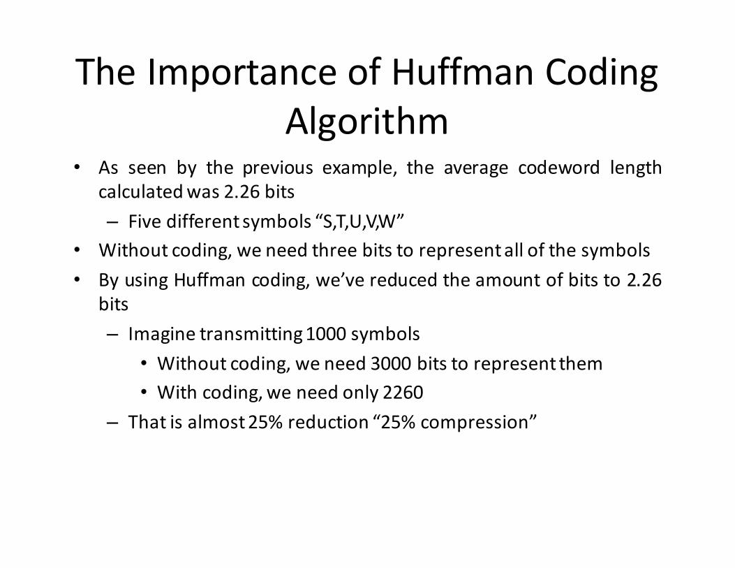
The Importance of Huffman Coding
Algorithm• As seen by the previous example, the average codeword length
calculated was 2.26 bits
– Five different symbols “S,T,U,V,W”
• Without coding, we need three bits to represent all of the symbols
• By using Huffman coding, we’ve reduced the amount of bits to 2.26
bits
– Imagine transmitting 1000 symbols
• Without coding, we need 3000 bits to represent them
• With coding, we need only 2260
– That is almost 25% reduction “25% compression”
Chapter 4: Channel Encoding
Abdullah Al-Meshal
Overview
• Channel encoding definition and importance
• Error Handling techniques
• Error Detection techniques
• Error Correction techniques
Channel Encoding - Definition
• In digital communication systems an optimum
system might be defined as one that
minimizes the probability of bit error.
• Error occurs in the transmitted signal due to
the transmission in a non-ideal channel
– Noise exists in channels
– Noise signals corrupt the transmitted data
Channel Encoding - Imporatance
• Channel encoding
– Techniques used to protect the transmitted signal
from the noise effect
• Two basic approaches of channel encoding
– Automatic Repeat Request (ARQ)
– Forward Error Correction (FEC)
Automatic Repeat Request (ARQ)
• Whenever the receiver detects an error in thetransmitted block of data, it requests thetransmitter to send the block again toovercome the error.
• The request continue “repeats” until the blockis received correctly
• ARQ is used in two-way communicationsystems
– Transmitter � Receiver
Automatic Repeat Request (ARQ)
• Advantages:
– Error detection is simple and requires much
simpler decoding equipments than the other
techniques
• Disadvantages:
– If we have a channel with high error rate, the
information must be sent too frequently.
– This results in sending less information thus
producing a less efficient system
Forward Error Correction (FEC)
• The transmitted data are encoded so that thereceiver can detect AND correct any errors.
• Commonly known as Channel Encoding
• Can be Used in both two-way or one-waytransmission.
• FEC is the most common technique used inthe digital communication because of itsimproved performance in correcting theerrors.
Forward Error Correction (FEC)
• Improved performance because:
– It introduces redundancy in the transmitted data in a controlled way
– Noise averaging : the receiver can average out the noise over long time of periods.
Error Control Coding
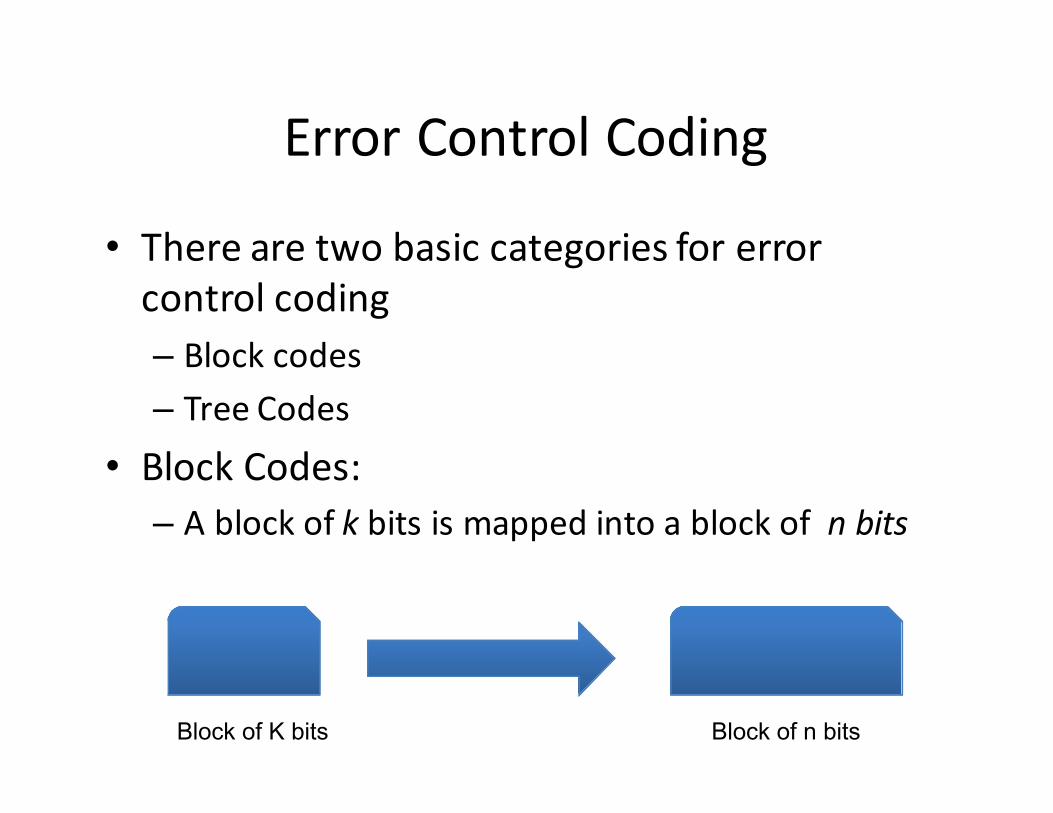
• There are two basic categories for error
control coding
– Block codes
– Tree Codes
• Block Codes:
– A block of k bits is mapped into a block of n bits
Block of K bits Block of n bits
Error Control Coding
• tree codes are also known as codes with
memory, in this type of codes the encoder
operates on the incoming message sequence
continuously in a serial manner.
• Protecting data from noise can be done
through:
– Error Detection
– Error Correction

Error Control Coding
• Error Detection
– We basically check if we have an error in the
received data or not.
• There are many techniques for the detection
stage
• Parity Check
• Cyclic Redundancy Check (CRC)
Error Control Coding
• Error Correction
– If we have detected an error “or more” in the
received data and we can correct them, then we
proceed in the correction phase
• There are many techniques for error
correction as well:
• Repetition Code
• Hamming Code
Error Detection Techniques
• Parity Check
– Very simple technique used to detect errors
• In Parity check, a parity bit is added to the
data block
– Assume a data block of size k bits
– Adding a parity bit will result in a block of size k+1
bits
• The value of the parity bit depends on the
number of “1”s in the k bits data block
Parity Check
• Suppose we want to make the number of 1’s in the
transmitted data block odd, in this case the value of the parity
bit depends on the number of 1’s in the original data
– if we a message = 1010111
• k = 7 bits
– Adding a parity check so that the number of 1’s is even
• The message would be : 10101111
• k+1 = 8 bits
• At the reciever ,if one bit changes its values, then an error can
be detected
Example - 1
• At the transmitter, we need to send the
message M= 1011100.
– We need to make the number of one’s odd
• Transmitter:
– k=7 bits , M =1011100
– k+1=8 bits , M’=10111001
• Receiver:
– If we receive M’ = 10111001 � no error is
detected
– If we receive M’= 10111000 � an Error is
detected
Parity Check
• If an odd number of errors occurred, then the
error still can be detected “assuming a parity
bit that makes an odd number of 1’s”
• Disadvantage:
– If an even number of errors occurred, the the
error can NOT be detected “assuming a parity bit
that makes an odd number of 1’s”
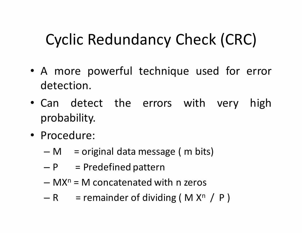
Cyclic Redundancy Check (CRC)
• A more powerful technique used for error
detection.
• Can detect the errors with very high
probability.
• Procedure:
– M = original data message ( m bits)
– P = Predefined pattern
– MXn = M concatenated with n zeros
– R = remainder of dividing ( M Xn / P )
Sender Operation
• Sender
• The transmitter performs the division M / P
• The transmitter then computes the remainder R
• It then concatenates the remainder with the message
“M:R”
• Then it sends the encoded message over the channel
“M:R”.
• The channel transforms the message M:R into M’:R’
Receiver Operation
• Receiver:
– The receiver receives the message M’:R’
– It then performs the division of the message by
the predetermined pattern P, “ M’:R’ / P ”
• If the remainder is zero, then it assumes the message is
not corrupted “Does not have any error”. Although it
may have some.
• If the remainder is NON-zero, then for sure the
message is corrupted and contain error/s.
Division process
• The division used in the CRC is a modulo-2
arithmetic division.
• Exactly like ordinary long division, only
simpler, because at each stage we just need to
check whether the leading bit of the current
three bits is 0 or 1.
– If it's 0, we place a 0 in the quotient and
exclusively OR the current bits with zeros.
– If it's 1, we place a 1 in the quotient and
exclusively OR the current bits with the divisor.

Example - 2
• Using CRC for error detection and given a
message M = 10110 with P = 110, compute
the following
– Frame check Sum (FCS)
– Transmitted frame
– Received frame and check if there is any error in
the data
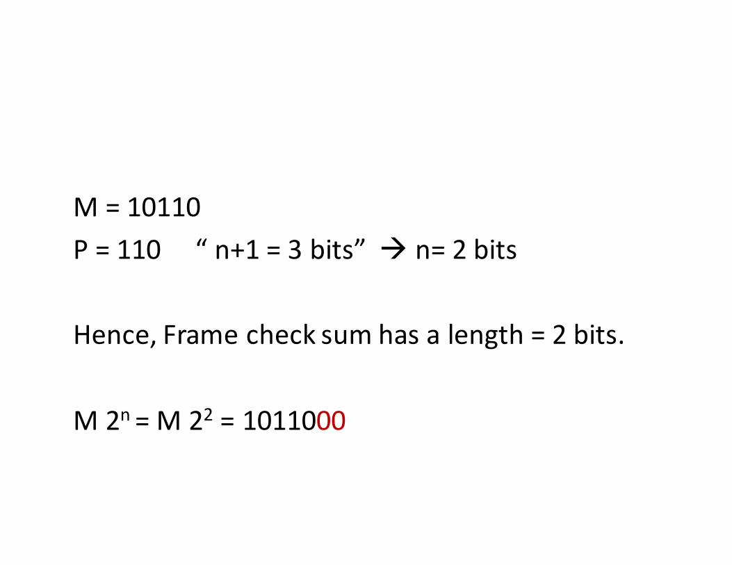
M = 10110
P = 110 “ n+1 = 3 bits” � n= 2 bits
Hence, Frame check sum has a length = 2 bits.
M 2n = M 22 = 1011000
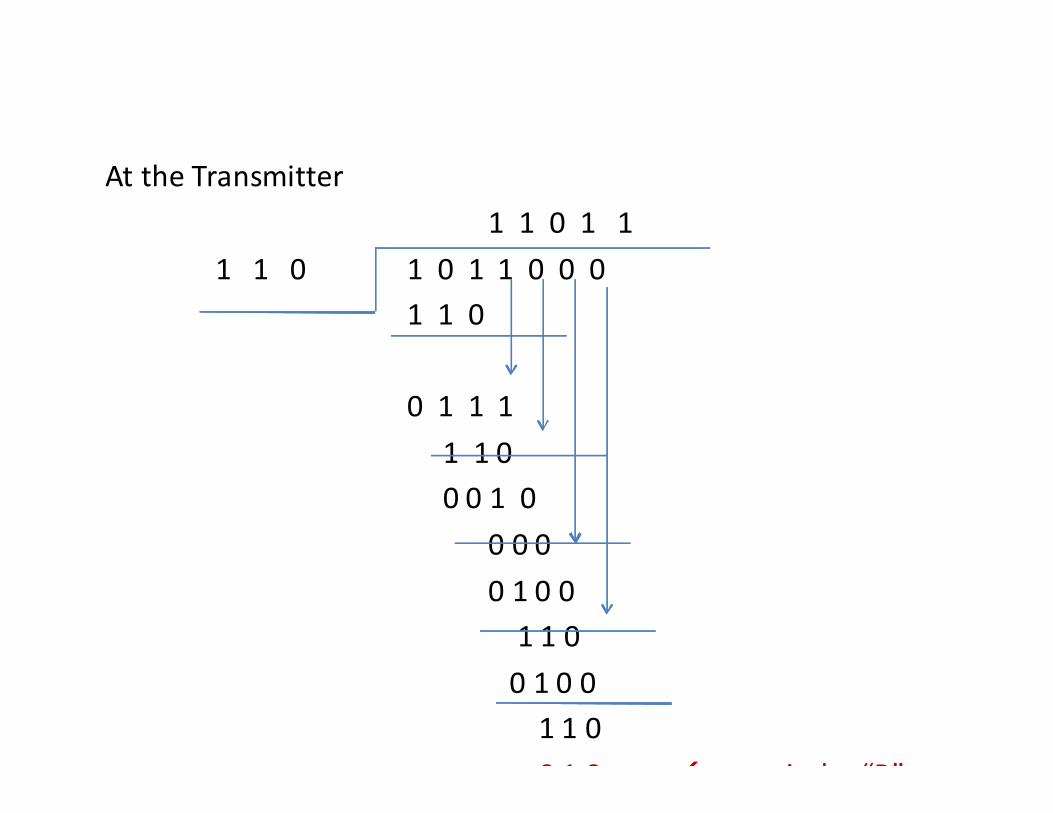
At the Transmitter
1 1 0 1 1
1 1 0 1 0 1 1 0 0 0
1 1 0
0 1 1 1
1 1 0
0 0 1 0
0 0 0
0 1 0 0
1 1 0
0 1 0 0
1 1 0
0 1 0 remainder “R”
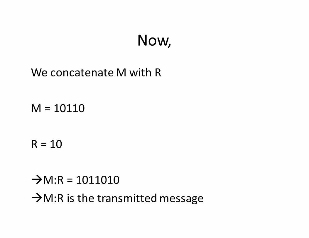
Now,
We concatenate M with R
M = 10110
R = 10
�M:R = 1011010
�M:R is the transmitted message

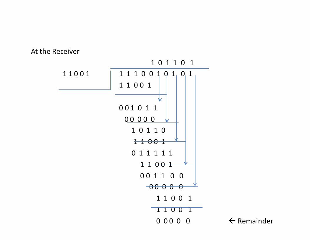
At the Receiver
1 1 0 1 1
1 1 0 1 0 1 1 0 1 0
1 1 0
0 1 1 1
1 1 0
0 0 1 0
0 0 0
0 1 0 1
1 1 0
0 1 1 0
1 1 0
0 0 0 remainder “R”
• Since there is no remainder at the receiver,
the we can say that the message is not
corrupted “i.e. does not contain any errors”
• If the remainder is not zero, then we are sure
that the message is corrupted.
Example - 3
• Let M = 111001 and P = 11001
• Compute the following:
– Frame check Sum (FCS)
– Transmitted frame
– Received frame and check if there is any error in
the data
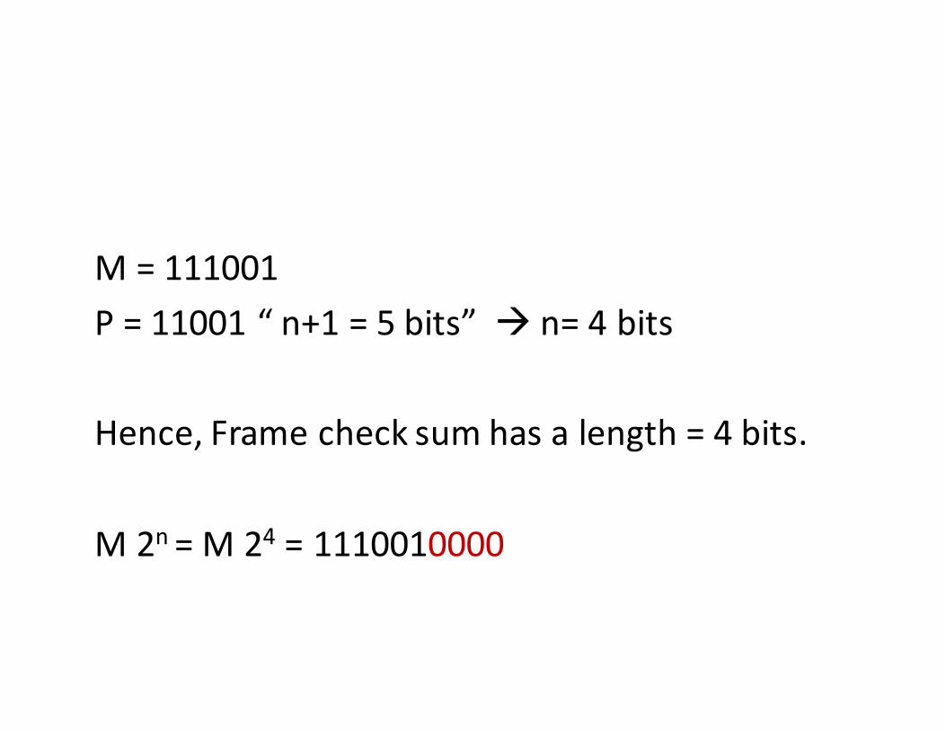
M = 111001
P = 11001 “ n+1 = 5 bits” � n= 4 bits
Hence, Frame check sum has a length = 4 bits.
M 2n = M 24 = 1110010000
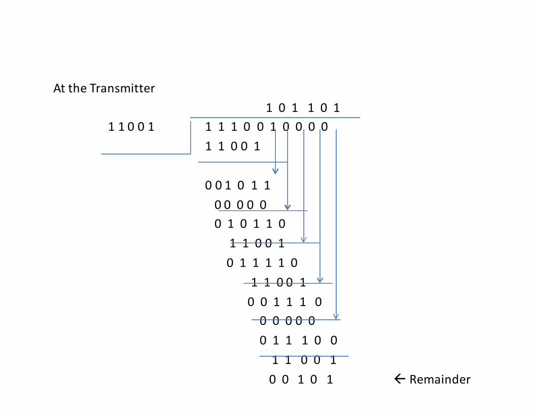
At the Transmitter
1 0 1 1 0 1
1 1 0 0 1 1 1 1 0 0 1 0 0 0 0
1 1 0 0 1
0 0 1 0 1 1
0 0 0 0 0
0 1 0 1 1 0
1 1 0 0 1
0 1 1 1 1 0
1 1 0 0 1
0 0 1 1 1 0
0 0 0 0 0
0 1 1 1 0 0
1 1 0 0 1
0 0 1 0 1 Remainder
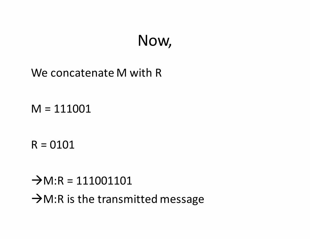
Now,
We concatenate M with R
M = 111001
R = 0101
�M:R = 111001101
�M:R is the transmitted message
At the Receiver
1 0 1 1 0 1
1 1 0 0 1 1 1 1 0 0 1 0 1 0 1
1 1 0 0 1
0 0 1 0 1 1
0 0 0 0 0
1 0 1 1 0
1 1 0 0 1
0 1 1 1 1 1
1 1 0 0 1
0 0 1 1 0 0
0 0 0 0 0
1 1 0 0 1
1 1 0 0 1
0 0 0 0 0 Remainder
Chapter 5:
Modulation Techniques
Abdullah Al-Meshal
Introduction
• After encoding the binary data, the data is
now ready to be transmitted through the
physical channel
• In order to transmit the data in the physical
channel we must convert the data back to an
electrical signal
– Convert it back to an analog form
• This process is called modulation
Modulation - Definition
• Modulation is the process of changing aparameter of a signal using another signal.
• The most commonly used signal type is thesinusoidal signal that has the form of :
•V(t) = A sin ( wt + θ )
• A : amplitude of the signla
• w : radian frequency
• θ : Phase shift
Modulation
• In modulation process, we need to use twotypes of signals:
– Information, message or transmitted signal
– Carrier signal
• Let’s assume the carrier signal is of asinusoidal type of the form x(t) = A sin (wt + θ)
• Modulation is letting the message signal tochange one of the carrier signal parameters
Modulation
• If we let the carrier signal amplitude changes
in accordance with the message signal then
we call the process amplitude modulation
• If we let the carrier signal frequency changes
in accordance with the message signal then
we call this process frequency modulation
Digital Data Transmission
• There are two types of Digital Data
Transmission:
1) Base-Band data transmission– Uses low frequency carrier signal to transmit the data
2) Band-Pass data transmission– Uses high frequency carrier signal to transmit the data
Base-Band Data Transmission
• Base-Band data transmission = Line coding
• The binary data is converted into an electrical
signal in order to transmit them in the channel
• Binary data are represented using amplitudes
for the 1’s and 0’s
• We will presenting some of the common base-
band signaling techniques used to transmit
the information
Line Coding Techniques
• Non-Return to Zero (NRZ)
• Unipolar Return to Zero (Unipolar-RZ)
• Bi-Polar Return to Zero (Bi-polar RZ)
• Return to Zero Alternate Mark Inversion (RZ-AMI)
• Non-Return to Zero – Mark (NRZ-Mark)
• Manchester coding (Biphase)
Non-Return to Zero (NRZ)
• The “1” is represented by some level
• The “0” is represented by the opposite
• The term non-return to zero means the signal
switched from one level to another without
taking the zero value at any time during
transmission.
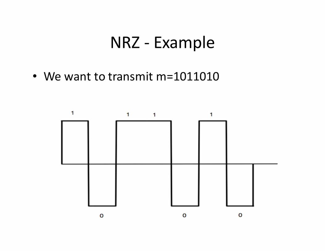
NRZ - Example
• We want to transmit m=1011010

Unipolar Return to Zero (Unipolar RZ)
• Binary “1” is represented by some level that is
half the width of the signal
• Binary “0” is represented by the absence of
the pulse
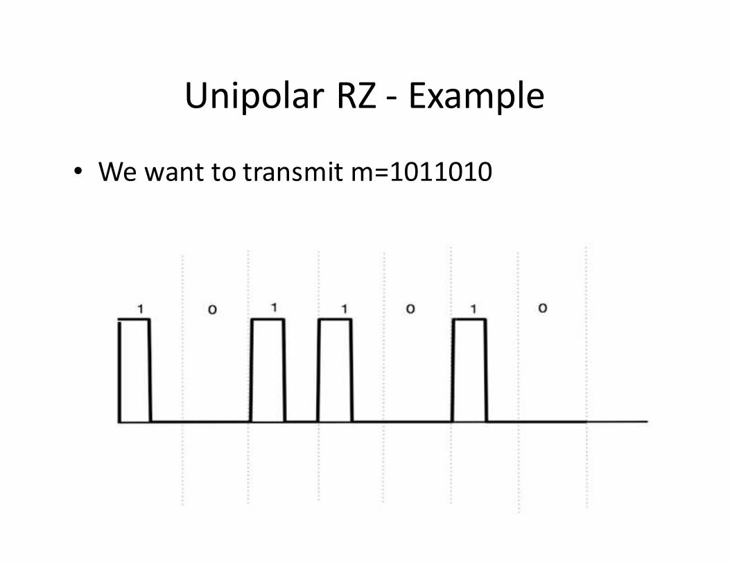
Unipolar RZ - Example
• We want to transmit m=1011010
Bipolar Return to Zero (Bipolar RZ)
• Binary “1” is represented by some level that is
half the width of the signal
• Binary “0” is represented a pulse that is half
width the signal but with the opposite sign
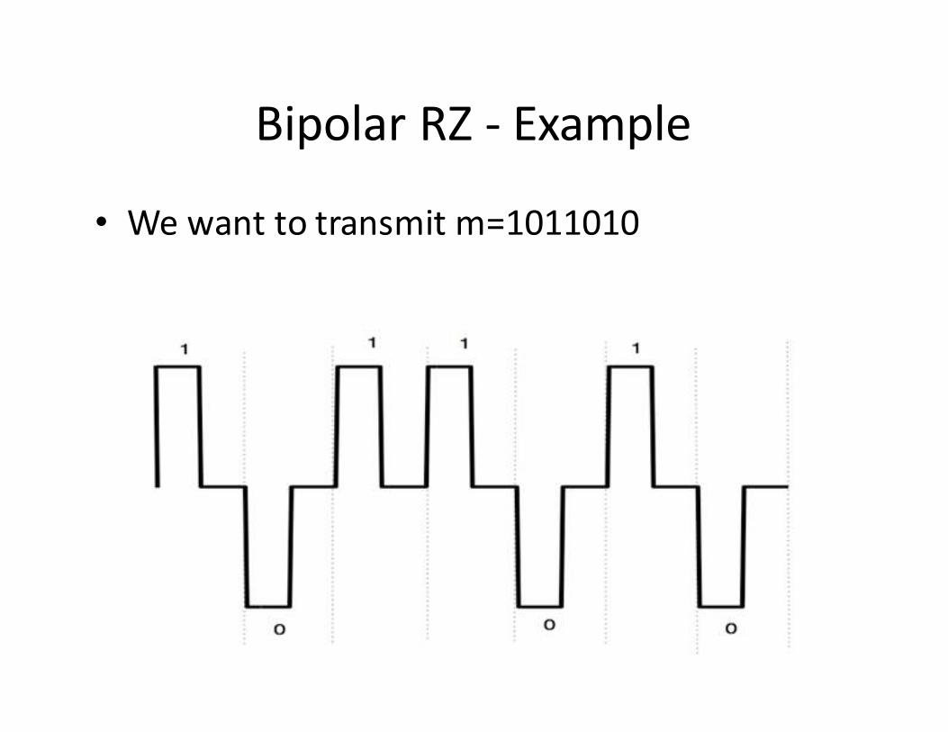
Bipolar RZ - Example
• We want to transmit m=1011010
Return to Zero Alternate Mark
Inversion (RZ-AMI)
• Binary “1” is represented by a pulse
alternating in sign
• Binary “0” is represented with the absence of
the pulse
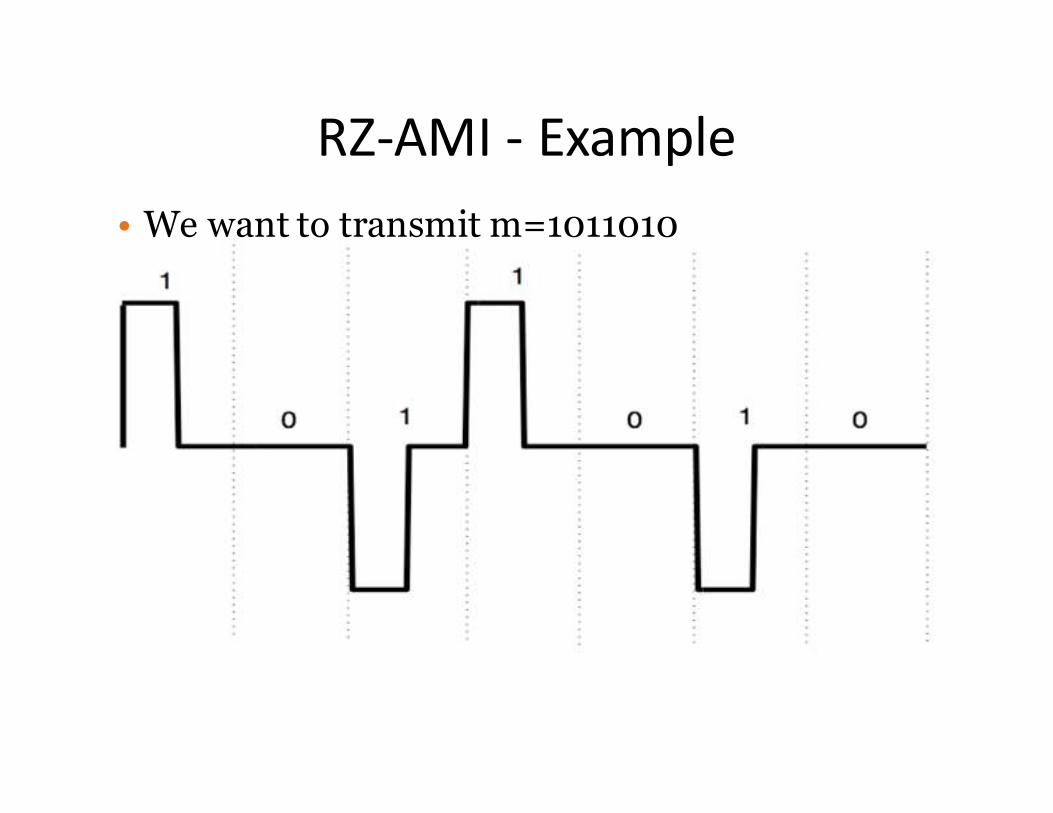
RZ-AMI - Example
• We want to transmit m=1011010
Non-Return to Zero – Mark (NRZ-Mark)
• Also known as differential encoding
• Binary “1” represented in the change of the
level
– High to low
– Low to high
• Binary “0” represents no change in the level
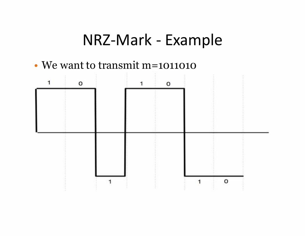
NRZ-Mark - Example
• We want to transmit m=1011010
Manchester coding (Biphase)
• Binary “1” is represented by a positive pulse
half width the signal followed by a negative
pulse
• Binary “0” is represented by a negative pulse
half width the signal followed by a positive
pulse
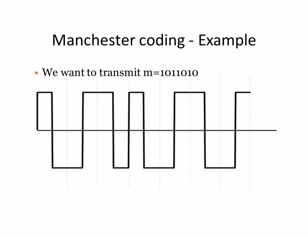
Manchester coding - Example
• We want to transmit m=1011010
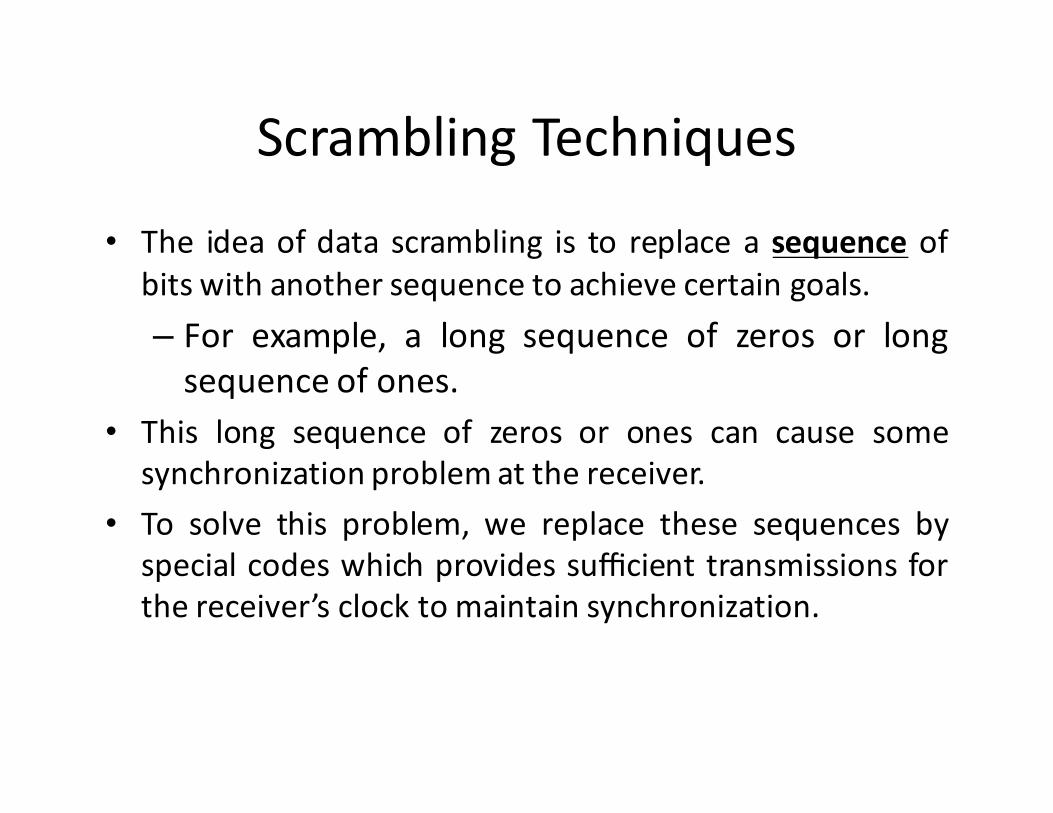
Scrambling Techniques
• The idea of data scrambling is to replace a sequence of
bits with another sequence to achieve certain goals.
– For example, a long sequence of zeros or long
sequence of ones.
• This long sequence of zeros or ones can cause some
synchronization problem at the receiver.
• To solve this problem, we replace these sequences by
special codes which provides sufficient transmissions for
the receiver’s clock to maintain synchronization.
Scrambling techniques
• We present two techniques used to replace a
long sequence of zeros by some special type
of sequences
– Bipolar 8 Zero substitution (B8ZS)
– High Density bipolar 3 Zeros (HDB3)
• Used in North America to replace sequences
with 8 zeros with a special sequence according
to the following rules:
• If an octet (8) of all zeros occurs and the last voltage
pulse preceding this octet was positive, then 000+-0-+
• If an octet of all zeros occurs and the last voltage pulse
preceding this octet was negative, then
000-+0+-
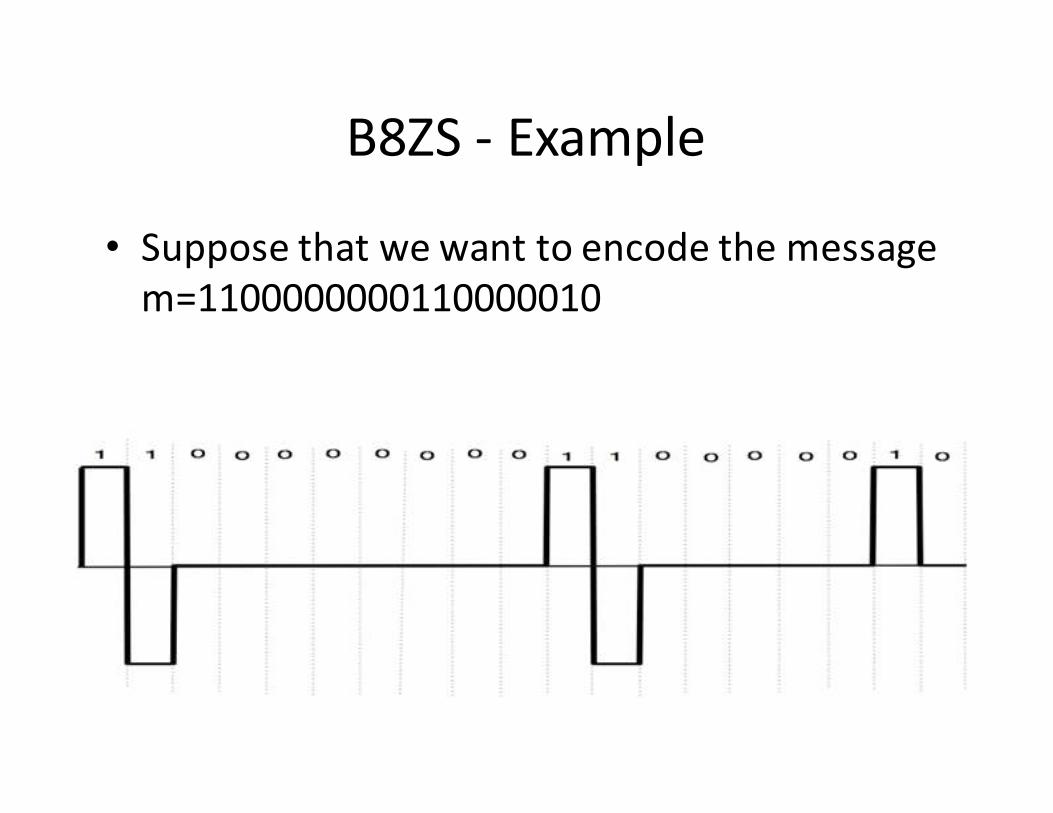
B8ZS - Example
• Suppose that we want to encode the message
m=1100000000110000010
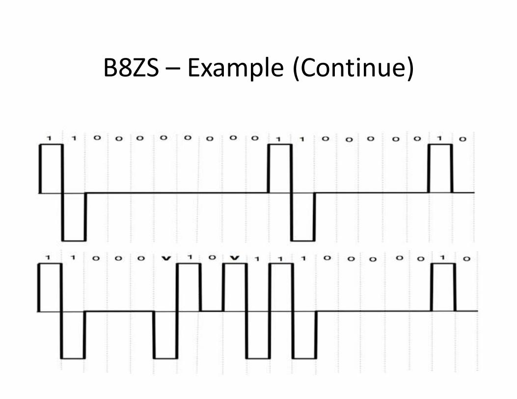
B8ZS – Example (Continue)
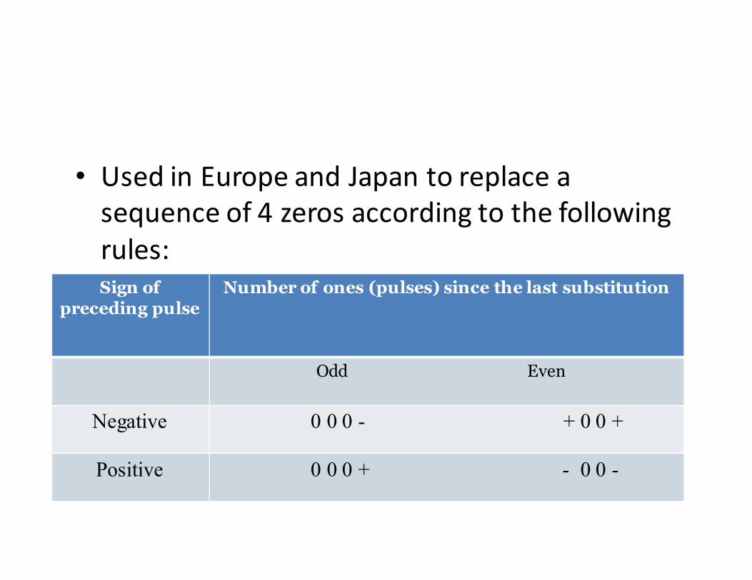
• Used in Europe and Japan to replace a
sequence of 4 zeros according to the following
rules:
Sign of
preceding pulse
Number of ones (pulses) since the last substitution
Odd Even
Negative 0 0 0 - + 0 0 +
Positive 0 0 0 + - 0 0 -
Transmission
• Transmission bandwidth: the transmission
bandwidth of a communication system is the
band of frequencies allowed for signal
transmission, in another word it is the band of
frequencies at which we are allowed to use to
transmit the data.
Bit Rate
• Bit Rate : is the number of bits transferred
between devices per second
• If each bit is represented by a pulse of width
Tb, then the bit rate
Rb =1
Tb bits /sec
Example – Bit rate calculation
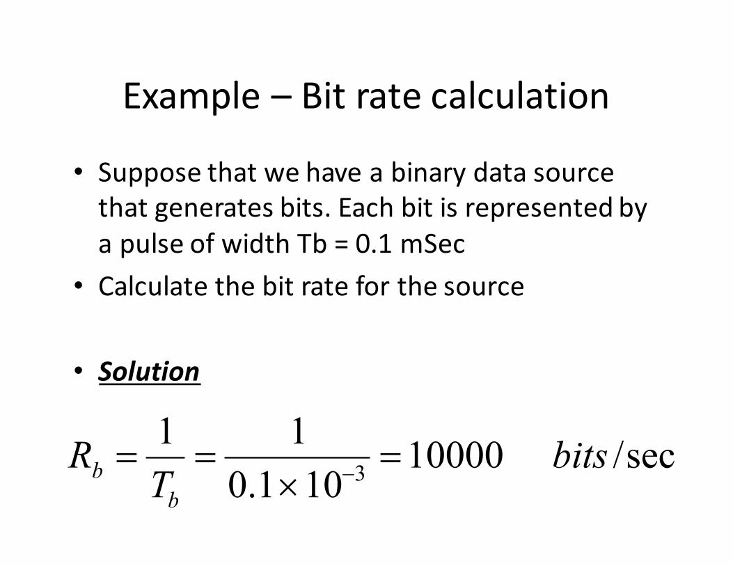
• Suppose that we have a binary data source
that generates bits. Each bit is represented by
a pulse of width Tb = 0.1 mSec
• Calculate the bit rate for the source
• Solution
Rb =1
Tb=
1
0.1×10−3=10000 bits /sec
Example – Bit rate calculation
• Suppose we have an image frame of size
200x200 pixels. Each pixel is represented by
three primary colors red, green and blue
(RGB). Each one of these colors is represented
by 8 bits, if we transmit 1000 frames in 5
seconds what is the bit rate for this image?
Example – Bit rate calculation
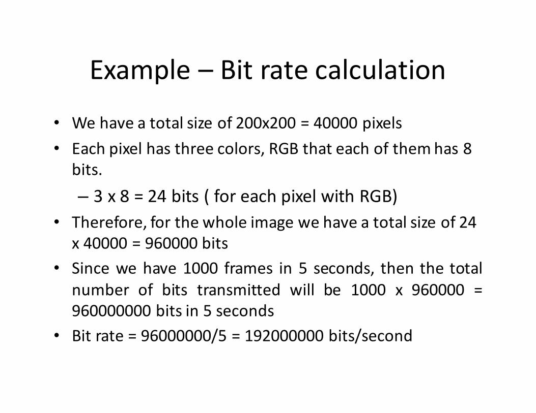
• We have a total size of 200x200 = 40000 pixels
• Each pixel has three colors, RGB that each of them has 8
bits.
– 3 x 8 = 24 bits ( for each pixel with RGB)
• Therefore, for the whole image we have a total size of 24
x 40000 = 960000 bits
• Since we have 1000 frames in 5 seconds, then the total
number of bits transmitted will be 1000 x 960000 =
960000000 bits in 5 seconds
• Bit rate = 96000000/5 = 192000000 bits/second
Baud rate (Symbol rate)
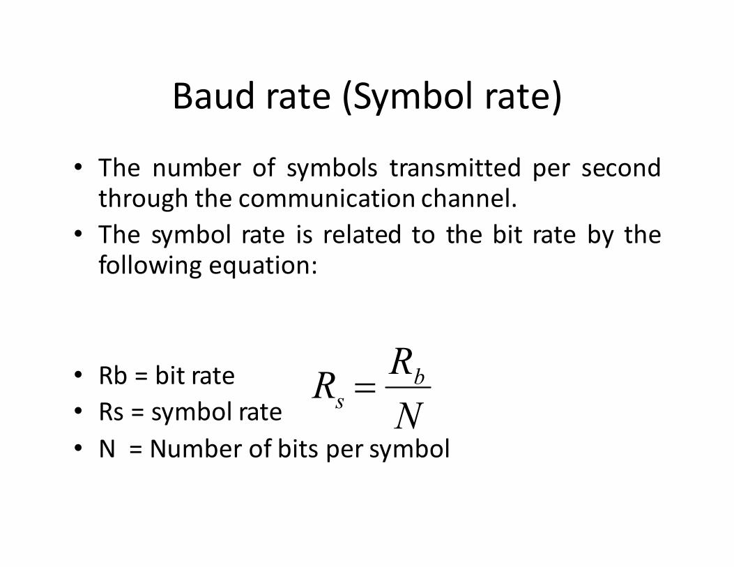
• The number of symbols transmitted per secondthrough the communication channel.
• The symbol rate is related to the bit rate by thefollowing equation:
• Rb = bit rate
• Rs = symbol rate
• N = Number of bits per symbol
Rs =Rb
N
Baud rate (Symbol rate)
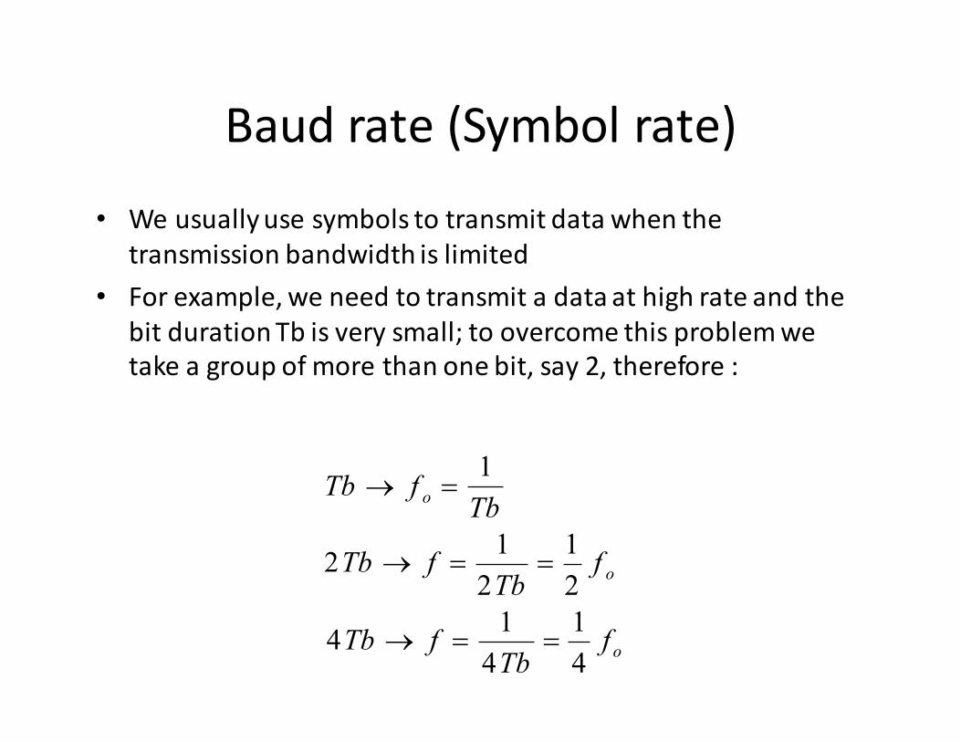
• We usually use symbols to transmit data when the
transmission bandwidth is limited
• For example, we need to transmit a data at high rate and the
bit duration Tb is very small; to overcome this problem we
take a group of more than one bit, say 2, therefore :
Tb → f o =1
Tb
2Tb → f =1
2Tb=1
2f o
4Tb → f =1
4Tb=1
4f o
Baud rate (Symbol rate)
• We notice that by transmitting symbols rather
than bits we can reduce the spectrum of the
transmitted signal.
• Hence, we can use symbol transmission rather
than bit transmission when the transmission
bandwidth is limited
Example
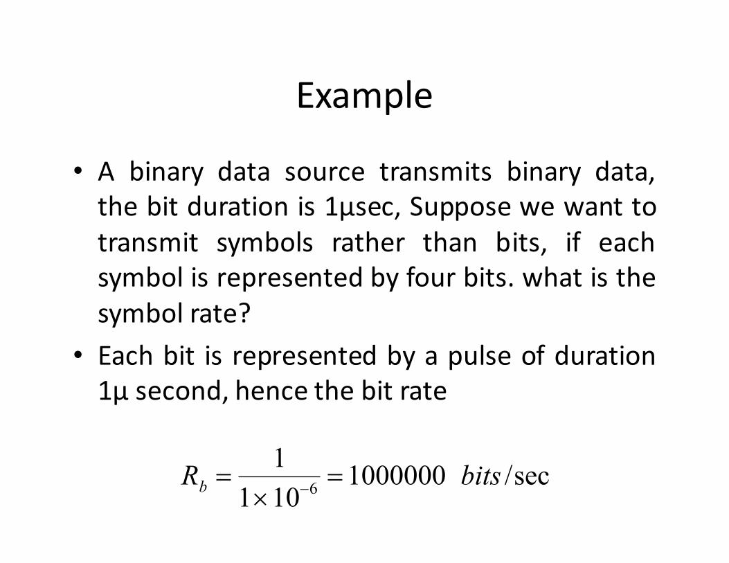
• A binary data source transmits binary data,
the bit duration is 1µsec, Suppose we want to
transmit symbols rather than bits, if each
symbol is represented by four bits. what is the
symbol rate?
• Each bit is represented by a pulse of duration
1µ second, hence the bit rate
Rb =1
1×10−6=1000000 bits /sec
Example (Continue)
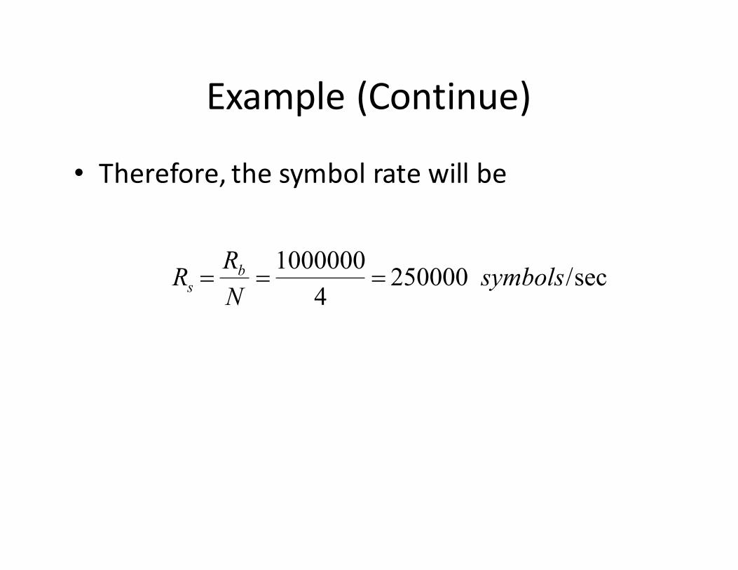
• Therefore, the symbol rate will be
Rs =Rb
N=1000000
4= 250000 symbols/sec
Chapter 5:
Modulation Techniques (Part II)
Abdullah Al-Meshal
Introduction
• Bandpass data transmission
• Amplitude Shift Keying (ASK)
• Phase Shift Keying (PSK)
• Frequency Shift Keying (FSK)
• Multilevel Signaling (Mary Modulation)
Bandpass Data Transmission
• In communication, we use modulation for several reasons in particular:
– To transmit the message signal through the communication channel efficiently.
– To transmit several signals at the same time over acommunication link through the process ofmultiplexing or multiple access.
– To simplify the design of the electronic systems usedto transmit the message.
– by using modulation we can easily transmit data withlow loss
Bandpass Digital Transmission
• Digital modulation is the process by whichdigital symbols are transformed into wave-forms that are compatible with thecharacteristics of the channel.
• The following are the general steps used bythe modulator to transmit data– 1. Accept incoming digital data
– 2. Group the data into symbols
– 3. Use these symbols to set or change the phase, frequency oramplitude of the reference carrier signal appropriately.
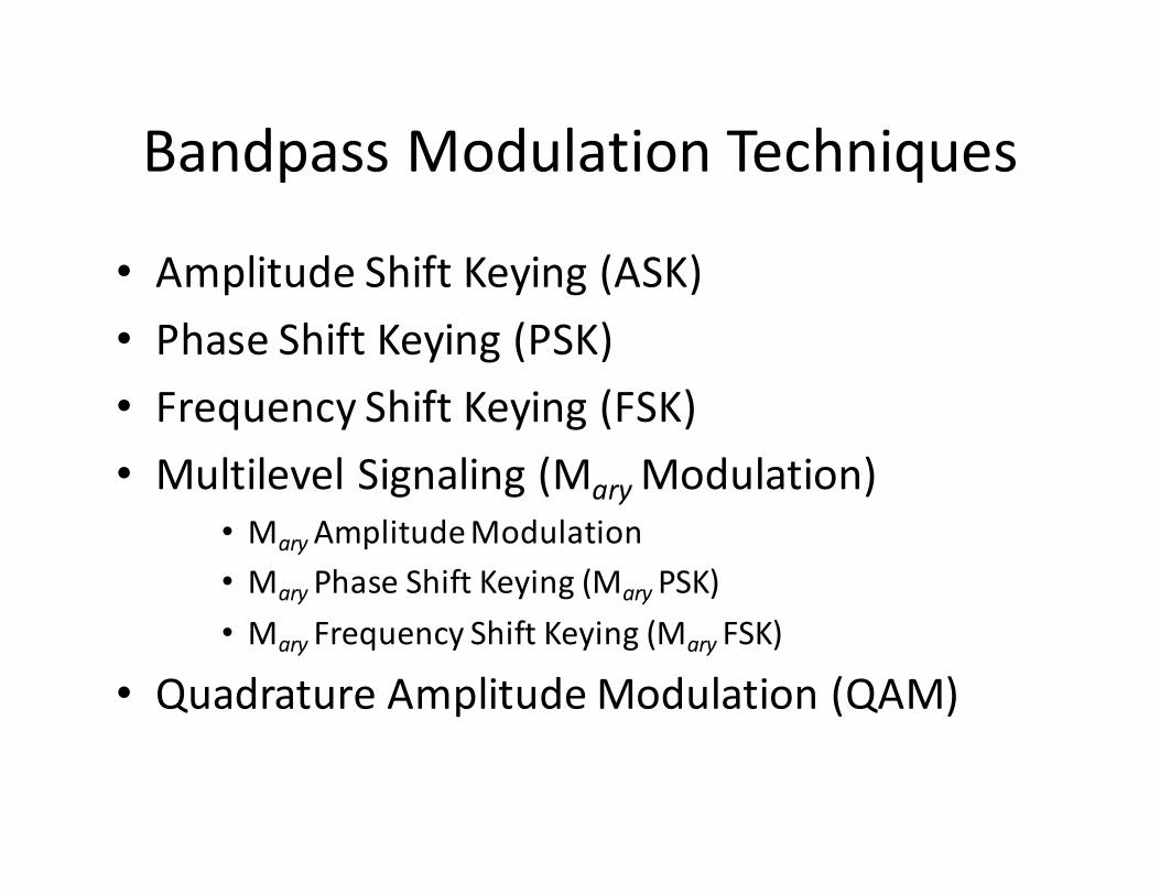
Bandpass Modulation Techniques
• Amplitude Shift Keying (ASK)
• Phase Shift Keying (PSK)
• Frequency Shift Keying (FSK)
• Multilevel Signaling (Mary Modulation)
• Mary Amplitude Modulation
• Mary Phase Shift Keying (Mary PSK)
• Mary Frequency Shift Keying (Mary FSK)
• Quadrature Amplitude Modulation (QAM)
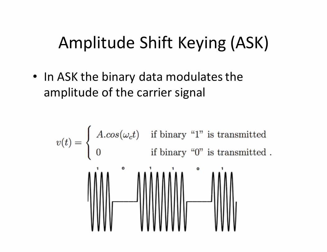
Amplitude Shift Keying (ASK)
• In ASK the binary data modulates the
amplitude of the carrier signal
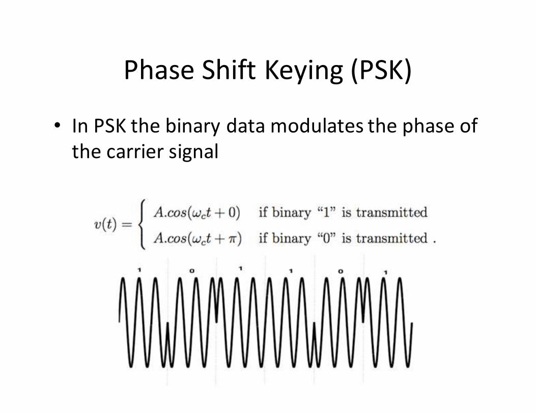
Phase Shift Keying (PSK)
• In PSK the binary data modulates the phase of
the carrier signal
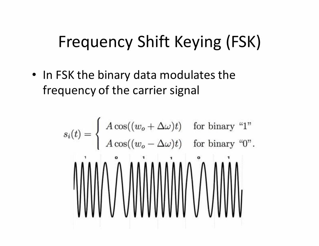
Frequency Shift Keying (FSK)
• In FSK the binary data modulates the
frequency of the carrier signal

Multilevel Signaling
(Mary Modulation)
• With multilevel signaling, digital inputs withmore than two modulation levels are allowedon the transmitter input.
• The data is transmitted in the form ofsymbols, each symbol is represented by k bits
–� We will have M=2K different symbol
• There are many different Mary modulation techniques,some of these techniques modulate one parameter likethe amplitude, or phase, or frequency
Mary Modulation
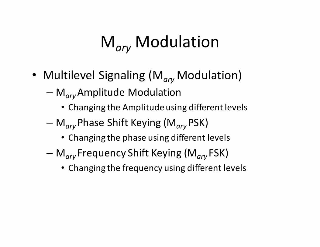
• Multilevel Signaling (Mary Modulation)
– Mary Amplitude Modulation
• Changing the Amplitude using different levels
– Mary Phase Shift Keying (Mary PSK)
• Changing the phase using different levels
– Mary Frequency Shift Keying (Mary FSK)
• Changing the frequency using different levels
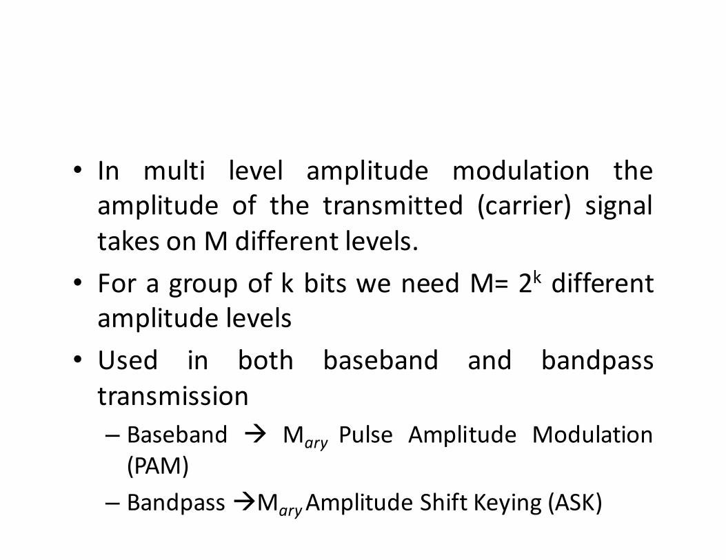
• In multi level amplitude modulation the
amplitude of the transmitted (carrier) signal
takes on M different levels.
• For a group of k bits we need M= 2k different
amplitude levels
• Used in both baseband and bandpass
transmission
– Baseband � Mary Pulse Amplitude Modulation
(PAM)
– Bandpass �Mary Amplitude Shift Keying (ASK)
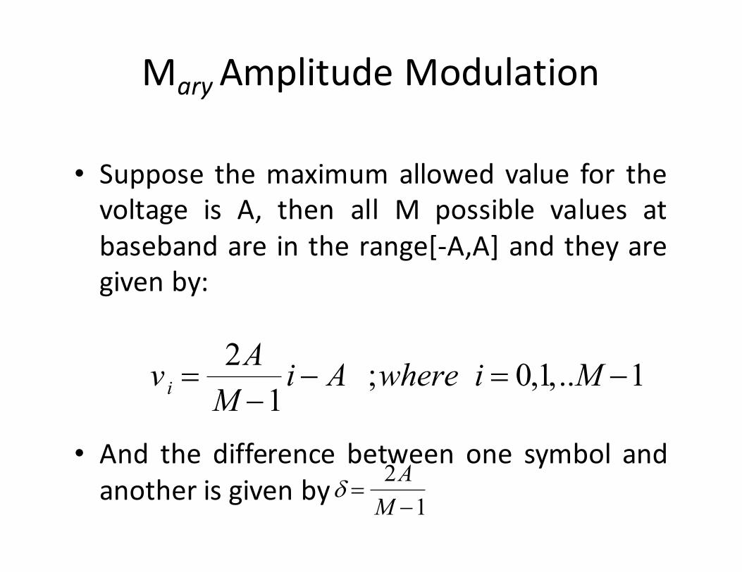
Mary Amplitude Modulation
• Suppose the maximum allowed value for the
voltage is A, then all M possible values at
baseband are in the range[-A,A] and they are
given by:
• And the difference between one symbol and
another is given by
v i =2A
M −1i − A ;where i = 0,1,..M −1
δ =2A
M −1
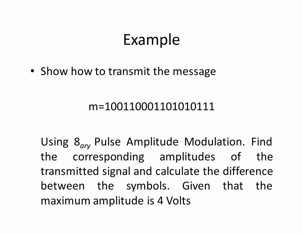
Example
• Show how to transmit the message
m=100110001101010111
Using 8ary Pulse Amplitude Modulation. Find
the corresponding amplitudes of the
transmitted signal and calculate the difference
between the symbols. Given that the
maximum amplitude is 4 Volts
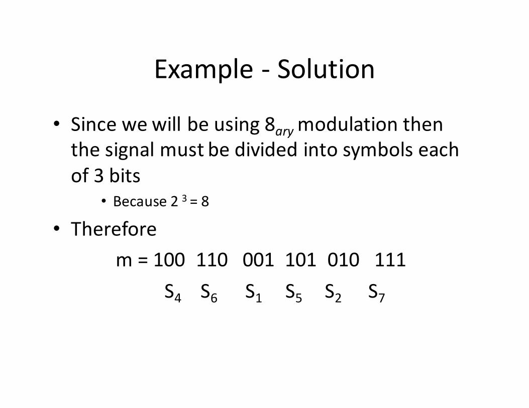
Example - Solution
• Since we will be using 8ary modulation then
the signal must be divided into symbols each
of 3 bits
• Because 2 3 = 8
• Therefore
m = 100 110 001 101 010 111
S4 S6 S1 S5 S2 S7
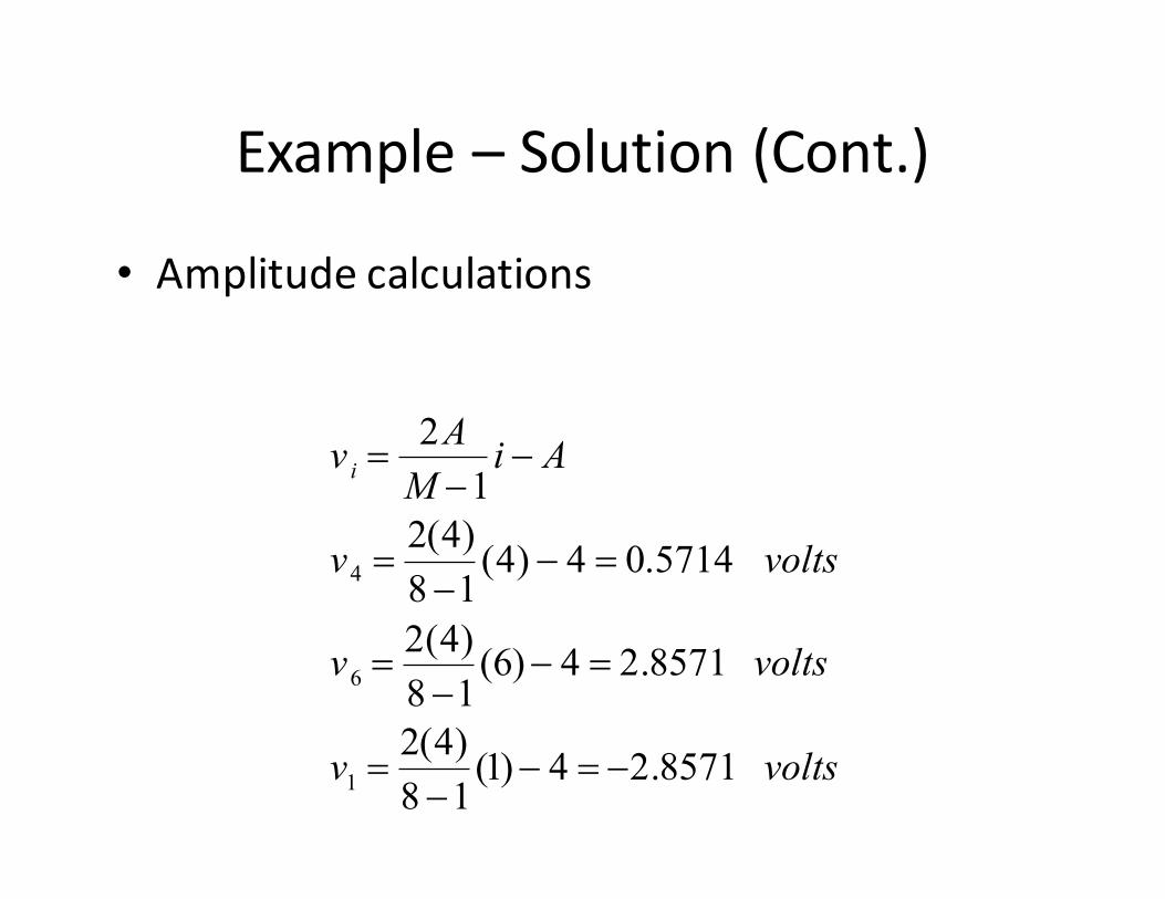
Example – Solution (Cont.)
• Amplitude calculations
v i =2A
M −1i − A
v4 =2(4)
8 −1(4) − 4 = 0.5714 volts
v6 =2(4)
8 −1(6)− 4 = 2.8571 volts
v1 =2(4)
8 −1(1)− 4 = −2.8571 volts
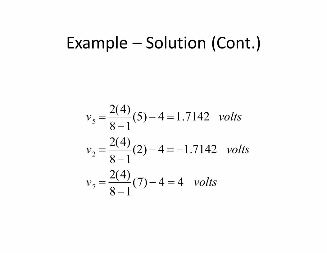
Example – Solution (Cont.)
v5=2(4)
8 −1(5) − 4 =1.7142 volts
v2=2(4)
8 −1(2) − 4 = −1.7142 volts
v7=2(4)
8 −1(7) − 4 = 4 volts
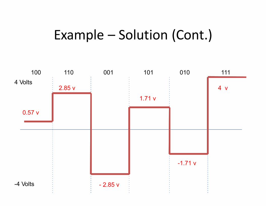
Example – Solution (Cont.)
4 Volts
-4 Volts
100 110 001 101 010 111
0.57 v
2.85 v
- 2.85 v
1.71 v
-1.71 v
4 v
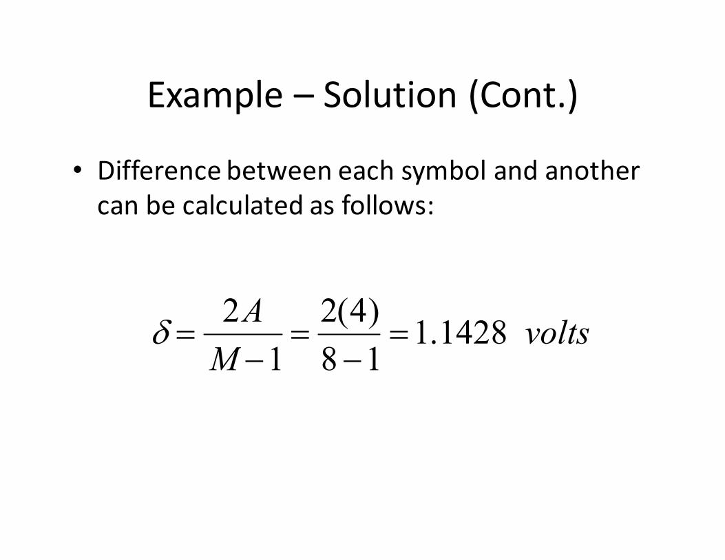
Example – Solution (Cont.)
• Difference between each symbol and another
can be calculated as follows:
δ =2A
M −1=2(4)
8−1=1.1428 volts