fundamentals and the origin of fama-french factors: the...

426 Finance a úvěr-Czech Journal of Economics and Finance, 60, 2010, no. 5

JEL Classification: G12 Keywords: Fama and French (1993) factors, fundamentals, rational pricing

Fundamentals and the Origin of Fama-French Factors: The Case of the Spanish Market* Francisco J. De PEÑA – University of Navarra, Spain Carlos FORNER – University of Alicante, Spain ([email protected]) (corresponding author) Germán LÓPEZ-ESPINOSA – University of Navarra, Spain

Abstract The interpretation of the Fama and French SMB and HML factors (Fama and French, 1993) as risk factors is an unresolved question that has carried a lot of controversy in the asset-pricing literature and it is far from being solved. The aim of this study is to con-tribute to the understanding of this issue by analyzing a rational pricing explanation of this model in the Spanish stock market. There is no empirical evidence concerning the relation between returns and fundamentals in this capital market, therefore it is nec-essary to study this relation in order to evaluate whether the use of this model is sup-ported by a rational pricing explanation in non-U.S. markets. Following the Fama and French (1995) approach we analyze whether there are size and book-to-market factors in fundamentals similar to those observed in returns and whether these factors in funda-mentals drive stock returns. Our results show that there are factors in fundamentals similar to those observed in returns. Secondly, when return on capital is used as a proxy for fundamentals, factors in fundamentals drive factors in returns. Therefore, return on capital is a useful fundamental variable used by investors in the Spanish stock market. These results give support to the use of this model in the Spanish capital market.

1. Introduction The CAPM (Capital Asset Pricing Model) is one of the most important build-

ing blocks of modern finance. According to this theory-based model, the return required on an investment (and its expected return in an efficient market) is a positive function of an overall risk factor: the market beta. This model allows researchers and practitioners to estimate expected returns in order to compute abnormal returns, the cost of capital of a firm, and so on.

If this model is correct it should explain why stocks yield different average returns. However, there is extensive U.S. evidence that the market beta is not able to fully capture the cross-sectional differences in average stock returns in the way the CAPM model predicts. However, the average stock returns seem to be highly related to some stock characteristics such as size and fundamental/market ratios. Fama and French (1992, 1993) show that size and book-to-market (hereafter BM) characteristics play a dominant role in capturing the cross-section of stock returns, and suggest an extension of the CAPM that includes two additional factors: a small-

* This work has received financial aid from the Subdirección General de Proyectos de Investigación del Ministerio de Ciencia e Innovación, through project ECO2008-02599/ECON, from the Dirección General de Investigación y Transferencia Tecnológica de la Conselleria d’Empresa, Universitat i Ciencia, throughproject GVPRE/2008/190, and from the Universidad de Navarra (PIUNA).

Finance a úvěr-Czech Journal of Economics and Finance, 60, 2010, no. 5 427

-minus-big (SMB) zero-cost portfolio, which is based on firm size, and a high-minus- -low zero-cost portfolio based on the BM value of the stock. Fama and French (1993) demonstrate that this three-factor model (hereafter the FF model) explains the av-eraged returns of U.S. stocks better than the CAPM. The good performance of this model has been confirmed in subsequent works (Fama and French, 1996; Lawrence et al., 2007).

There is also quite strong evidence that this model explains expected returns in widely different countries: Japan (Chan et al., 1991), countries in the euro area (Moerman, 20051), the Pacific Basin countries (Chui and Wei, 1998), Australia (Faff, 2004; Gaunt, 2004), Hong Kong (Nartea et al., 2008), China (Cao et al., 2005), and wider sets of countries (Fama and French, 1998; Griffin, 2002; Moerman, 2005).2 Furthermore, Gómez-Biscarri and López-Espinosa (2008) show that international versions of the FF model perform quite well if the accounting information is homo-geneous across firms.

In Spain there is also evidence supporting this model. Nieto and Rodríguez (2005) demonstrate that in the Spanish market the FF model has the best coefficient of determination among the static models, indicating that the SMB and HML factors provide valuable information. Moreover, the coefficient of determination improves in a conditional version of the model that includes state variables.

Given this growing empirical support of the FF model outperforming the CAPM, the FF model has become highly popular among academics and practitioners in order to make accurate estimates of expected returns. In Spain, for example, Forner and Marhuenda (2006) and Forner, Sanabria, and Marhuenda (2009) use the FF model to estimate the abnormal returns of the price and earnings momentum strategies and Matallín (2005) uses the FF model to measure mutual fund performance.

However, the correct interpretation of the results obtained with the FF model depends on whether the SMB and HML factors are actually proxying for some underlying risk factors and therefore are capturing the rational reward for supporting this risk. There exists a major controversy in the finance literature about whether the FF factors are proxying for some risk factors or, on the contrary, the good per-formance of this model is spurious or the effect of a mispricing story, with irrational investors driving stock prices.

This problem has warranted the attention of a considerable number of studies in the U.S. market but not in the non-U.S. market. The aim of this study is to fill this gap for the Spanish capital market. To do so we follow the Fama and French (1995) approach. Under the rational pricing story, stock prices are discounted expected net cash flows and the explanatory power of size and BM factors in returns must be driven by common factors in the shocks in these expected net cash flows. We can use shocks in expected earnings as proxies for the shocks to expected net cash flows, and changes in fundamentals as proxies for these shocks in expected earnings. Therefore, the common factors driving size and BM factors in returns should also have similar 1 However, Malin and Veeraraghavan (2004 and 2006) find different results for France, Germany, andthe United Kingdom. 2 Although Fama and French (1998) advocate a global version of their model, Griffin (2002) documentsthat the local versions work better (in terms of adjusted R2 and Jensen’s alpha) for the stock markets of the U.S., Canada, the UK, and Japan. Moerman (2005) also finds that even in the very integrated euro area, the domestic FF model outperforms the euro area FF model.


explanatory power in the change of fundamentals. So we must observe that dif-ferences in size and BM determine not only differences in returns, but also changes in fundamentals, that is, there are also size and BM factors in fundamentals. Finally, we should also expect size and BM factors in returns to be driven by these factors in fundamentals.

Furthermore, the considerable controversy regarding the origin of the FF factors highlights the need to accumulate out-of-sample evidence. The FF model needs further empirical verification before it can be accepted as a credible (ideally) theory-based model to replace the CAPM. This study also tries to contribute in this direction. There is little evidence of the fundamental-related FF (1995) approach being applied outside the U.S. Only Charitou and Constantinidis (2004) use this approach in the Japanese market, but their analysis is partial.

The rest of the paper proceeds as follows. Section 2 reviews the literature on the rationale of the FF model. Section 3 explains the methodology and data used in this work. Section 4 contains the results of the adequacy of this model for the Spanish capital market and Section 5 concludes.

2. The Rationale of Fama-French Factors Fama and French (1993, 1995) argue a rational-pricing story (that is, a risk-

-based explanation) of their SMB and HML factors. In the context of a multifactorial version of the Intertemporal Asset Pricing Model, ICAPM (Merton, 1973), or the Ar-bitrage Pricing Theory, APT (Ross, 1976), they state that the SMB and HML factors proxy for sensitivity to common risk factors3 in returns. The studies that show em-pirical evidence supporting this risk-based interpretation follow two different ap-proaches.

On the one hand, Fama and French (1995) – hereafter FF (1995) – test the ra-tional-pricing story by analyzing the relation of these factors with the underlying firm fundamentals. Following an APT interpretation, they argue that “if size and BM risk factors are the result of rational pricing, they must be driven by common factors in shocks to expected earnings that are related to size and BM”. They find that high BM firms tend to be persistently distressed and low BM firms are associated with sus-tained profitability, and small stocks tend to be less profitable than large stocks. They find that this evidence supports the use of these factors to measure undiversifiable comovement in returns.

On the other hand, Liew and Vassalou (2000) show that the SMB and HML portfolio returns contain significant information about future growth in GDP in sev-eral countries.4 In a later study, Vassalou and Xing (2004) conclude that size and BM effects are related to default risk and can be viewed as default effects. In the same line, Hahn and Lee (2006) find that changes in term and default yield spreads capture most of the systematic risks proxied by size and BM effects. Kelly (2003) presents 3 Size may proxy for default risk and BM may be an indicator of the relative prospects of firms. 4 Vassalou (2003) shows, however, that replacing the returns on the HML and SMB portfolios by their pre-dicted innovation in GDP leads to a significant degradation of the FF three-factor model power, meaning that the three-factor model power does not rest on the ability of the two hedge portfolios’ returns to predict GDP growth. Moreover, Moranaa and Beltratti (2006) observed structural breaks in the volatility of the FF factor portfolios that are incompatible with the absence of structural breaks in GDP growth and the change in the real rate of interest.


evidence from 18 countries that HML and SMB portfolios are correlated with future innovations in inflation and real economic growth.5 Brennan et al. (2001) find, using U.S. stock returns, that these portfolios do indeed have predictive power for both the real interest rate and the Sharpe ratio. Simpson and Ramchander (2008) show the ability of the FF three-factor model to capture information related to a number of macroeconomic variables, such as personal consumption and the consumer price index (CPI). All these results support the hypothesis that SMB and HML act as state variables of the ICAPM.

However, considerable controversy exists regarding the interpretation of SMB and HML as risk factors. Firstly, some studies question the goodness of the results obtained by the FF model, arguing that there are biases and econometric shortcom-ings in the procedures used to test the model, or simply that they are spurious. In this sense, Amihud et al. (1993) argue that potential survivorship can partially explain the magnitude of the BM variable and that by using generalized least squares (GLS) instead of ordinary least squares the importance of the market beta increases. Berk et al. (1999) and Gomes et al. (2003) argue problems in the measurement of beta. Berk (1995) suggests that high BM and small market capitalization firms will, by default, earn higher mean returns. Loughran (1997) finds that HML has little explanatory power once controls for seasonality, size, and exchange are included. Secondly, the FF model is strongly criticized because it is purely empirically motivated. There is no theory telling us what gives rise to SMB and HML factors. In this sense, Ferson et al. (1999) caution against using empirical regularities as explanatory risk factors.6

Moreover, some authors suggest a mispricing story. As with FF (1995), Lako-nishok et al. (1994) find that high fundamental/market stocks (including BM) tend to be distressed firms with persistently low earnings, and low fundamental/price stocks tend to be strong (growth) firms with persistently high earnings. But in contrast to FF (1995), Lakonishok et al. (1994) argue that the BM premium comes from the fact that investors are overly pessimistic about distressed stocks and overly optimistic about growth stocks; thus they over-extrapolate this performance to the future, underpricing (overpricing) distressed (growth) stocks. The posterior price adjustment will justify the BM premium.7 Another noteworthy study in this line is Daniel and Titman (1997), which shows that the characteristics, rather than the SMB and HML factor loadings, explain the cross-section in stock returns. This evidence is inconsistent with these factors reflecting common covariations in expected returns. Although Davis et al. (2000) contradict this evidence in the U.S. market using a longer sample, Daniel et al. (2001) find supportive evidence in the Japanese market for their characteristic argument. 5 Kelly (2003) includes the Spanish stock market, but this evidence is not supported in the Spanish case. 6 It must be also mentioned that other studies (Bhardwaj and Brooks, 1993; Jagannathan and Wang, 1996;Pettengill et al., 1995; Grundy and Malkiel, 1996; and Howton and Peterson, 1998) found evidence whichsuggests that allowing for beta instability and up-market versus down-market conditions has a potential role in explaining the Fama and French results. Jagannathan and Wang (1996) test a conditional CAPM that allows betas and market risk premiums to be time-varying, as well as including a measure of the re-turn on human capital as a component of the return on aggregate wealth. This model performs well, ex-plaining 57% of the cross-sectional variation and, more importantly, leaving relative size unable to explainthe remainder. 7 The Lakonishok et al. (1994) story is also supported in Japan (Cai, 1997; and Chang et al., 1995) andthe UK (Gregory et al., 2003).


The true story behind the SMB and HML factors is an open question that carries a lot of controversy in the asset-pricing literature and one which is far from being resolved. However, this model is broadly applied among academics and practitioners in order to make accurate estimates of expected stock returns (e.g. for portfolio selection problems, cost-of-capital calculations, capital budgeting, portfolio evaluation, and risk analysis decisions). The true origin of the Fama and French factors will affect, of course, the interpretation of studies that apply this model.

This drawback is also more important in non U.S. markets, where there is little or no evidence around the real origin of the Fama and French factors. It seems reasonable that, before applying this model in other countries, it is necessary to find if the factors proxy risk or not. However, this model has been applied in many dif-ferent countries without evaluating this concern.

3. Methodology and Data 3.1 Methodology

The goal of this study is to analyze the suitability of the FF (1993) model for the Spanish stock market. Therefore, we focus not on studying the performance of the model, but on whether this model captures differences in returns caused by dif-ferences in fundamentals. This would give support to the use of this model in non- -U.S. capital markets.

Following the approach of FF (1995), we analyze if differences in size and BM determine differences in fundamentals. In this work, we use different measures of profitability of a firm as proxies for the fundamentals. First, we use the standard return on assets (ROA) and return on equity (ROE) ratios:

EarningsROATotal Assets

EarningsROEBook Value

=

=

Following FF (1995), we use another version of the ROE ratio taking EBIT (earnings before interest and taxes) instead of earnings (net income) because EBIT is not affected by different levels of debt and differing tax rates.8

EBITROE

Book Value=

Another proxy for the fundamentals of a firm, used by FF (1995) and also in

this work, is the natural logarithm of sales ( )ln( )sales . On the other hand, Greenblatt (2005) describes two ratios to estimate the fun-

damentals of a firm. This author proposes ranking companies based on these two ratios (called “magic formulas”) in order to make large returns in the capital market. The ratios are the following: 8 The results presented in the paper are computed using the ROE ratio used by FF (1995) because this ratio is more robust for proxying the fundamentals of a firm. However, the results are similar using the standard ROE and they are available upon request.


EBITReturn on Capital =Net Working Capital + Net Fixed Assets

EBITEarnings Yield =Enterprise Value

EBIT is used in place of net income (earnings) because companies operate with different levels of debt and tax rates. The idea behind the first ratio, return on capital, is to compare current earnings from operations (EBIT) with the cost of the as-sets used to produce those earnings (tangible capital employed) computed as net working capital plus net fixed assets. In other words, the idea of this ratio is to figure out how much capital is needed to conduct the company’s business. As Greenblatt (2005) proposes and explains, goodwill is excluded from the tangible capital em-ployed.

The basic idea behind the second ratio is simple. The goal is to figure out how much a business earns relative to the purchase price of the business (enterprise value). The enterprise value of a company is computed as the sum of the market value of equity plus net interest-bearing debt.

The first step of the empirical analysis is to evaluate the factors in returns in the Spanish capital market; therefore, we run the following regression:

0 t t MKT t SMB t HML t tR RF MKT SMB HML eβ β β β− = + + + + (1)

where Rt is the return on the six size-BM portfolios (S/L, S/M, S/H, B/L, B/M, and B/H) in month t, tRF is the return on the risk-free asset, and te is an error term in month t, which we assume to be independent of the risk factors. MKTt is the market factor, computed as the difference between the market portfolio return and RF. SMB and HML factors are constructed as in FF (1993). SMB is the difference between the value-weighted average returns on the three portfolios containing the smallest cap stocks (S/L, S/M, and S/H) and the three portfolios containing the highest cap stocks (B/L, B/M, and B/H); and HML is the difference between the value-weighted av-erage returns on the two stock portfolios with a high BM ratio (S/H and B/H) and the portfolios with a low BM ratio (S/L and B/L).

Portfolios are based on size (classified as small or big relative to the median size) and on BM (classified as low, medium or high relative to the 30th and the 70th percentiles). Therefore, six portfolios are computed taking into account size and BM simultaneously.

Following the approach of FF (1995), we analyze if there is a pattern in fun-damentals similar to that observed in returns. The following regression is run for each portfolio and for each proxy for fundamentals (X = ROA, ROE, return on capi-tal, earnings yield, and natural logarithm of sales):

0 , , ,Δ Δ Δ Δ MKT MKT y SMB SMB y HML HML y yyX X X X eλ λ λ λ= + + + + (2)

where ΔXy is the mean annual change in a fundamental variable for a specific port-folio. ΔXMKT is the market factor in fundamentals: for X = ROA, ROE, return on capital, and earnings yield, the market is the mean taking into account all ob-


servations, and for sales it is the natural logarithm of total sales in the market, as in FF (1995). ΔXSMB, the size factor in ΔX, is the simple average of ΔX for the three small-stock portfolios (S/L, S/M, and S/H) minus the average for the three big-stock portfolios (B/L, B/M, and B/H). The BM factor in ΔX, ΔXHML, is the simple average of ΔX for the two stock portfolios with a high BM ratio (S/H and B/H) minus the av-erage for the two stock portfolios with a low BM ratio (S/L and B/L).

In the next step, in order to analyze if changes in fundamentals are captured by investors, the relation between returns and changes in fundamentals is studied with the following regression by each portfolio, factor, and proxy for the funda-mental:

Rt = α0 + α1DYLYy–1 + α2ΔXy + et (3)

where the dependent variables are the monthly returns in month t on the six size-BM portfolios (S/L, S/M, S/H, B/L, B/M, and B/H) and the market (MKT), size (SMB), and BM (HML) factors in returns. DYLYy–1 is the dividend yield of the value-weighted portfolio on the Spanish stock market for year y-1. ΔXy is the mean annual change in a fundamental variable for a specific portfolio divided by 12.9 As DYLY and ΔX are year-frequency data, they remain constant from January to December. For example, for R01/2000 to R12/2000 the explicative variables are the dividend yield computed at the end of 1999 and the change in the fundamental variable from 1999 to 2000.10

Since rational stock prices are discounted expected future earnings, if size and BM-related factors in returns are the result of rational pricing, then they must be driven by these factors in fundamentals. This question is analyzed by running the fol-lowing regression: Rt = γ0 + γDYLYDYLYy–1 + γMKTΔXMKT,y + γSMBΔXSMB,y + γHMLΔXHML,y + et (4)

where the dependent variables in the regression are the returns in month t on the six size-BM portfolios (S/L, S/M, S/H, B/L, B/M, and B/H).

3.2 Data The sample consists of 162 non-financial stocks quoted in the Spanish stock

market during the period January 1991 to December 2004. We ignore financial com-panies – banks and insurance companies – because their different leverage could disturb the results when forming portfolios with non-financial companies.

We form portfolios based on BM and size. When we form portfolios based on BM, we remove the companies with negative BM values. Regarding size, firm size or market value is measured as the number of outstanding shares times the stock closing price on the last trading day in June. The dividend yield of a portfolio is computed as the sum of stock dividends from January to December of year y divided 9 This implies that the accounting numbers have been generated in a uniform way during the year. 10 In contradistinction to FF (1995) we run this regression with monthly observations. As the explicative variables are year-frequency they remain constant during the year. Moreover, we use ΔXy instead of ΔXy+1.However, as we use monthly observations, we keep, to some extent, the one-year-ahead spirit of the re-gression used by FF (1995). For example, for the January return of year y the explicative variable isthe change in the fundamental from December year y-1 to December year y. Given that our sample period is somewhat shorter than the one studied by FF (1995), using yearly observations instead of monthlywould mean running the regression with only 11 observations.


by the sum of stock market equity in December year y. When needed, the 12-month Spanish Treasury Bills interest rate is taken as the risk free rate.

The portfolios are formed and updated every June 30th of year y, and we com-pute value weighted monthly returns from July year y to June year y+1. Following FF (1995), we choose June 30th because most firms end the fiscal year in December and they do not present their audited annual reports to shareholders until June 30th. Even taking into account possible delays in the process, by the end of June the accounting information of the firms should be available for all investors in the market and they should be able to make their investment decisions based on such audited information. We follow the same procedure as explained in Fama and French (1993 and 1995).

Throughout this paper, we form different ratios based on financial and account-ing measures: return on assets (ROA), return on equity (ROE), return on capital, and earnings yield. Whenever we compute profitability ratios, we compute the ratio of the corresponding earnings measure in year y to the corresponding company value in year y-1. We call this Xy.

The accounting data used to compute these ratios comes from the Spanish Se-curities and Exchange Commission database, available on its website (www.cnmv.es). Hence, we take sales, net income, EBIT, total assets, equity or book value, and net working capital. The concept of net fixed assets used by Greenblatt (2005) had to be adapted to local Spanish accounting standards. Total debt is the difference between total assets and equity.

4. Results 4.1 Persistence of Fama and French Factors Based on Profitability

Following a simple dividend discount model, FF (1995) demonstrate that high BM should be associated with a persistently low ratio of earnings to book equity, while low BM should be associated with persistently strong ratio of earnings to book equity.

In untabulated results (we do not report all the persistence analyses in order to save space), we obtain results consistent with the prediction of FF (1995) when we use different proxies for economic fundamentals.

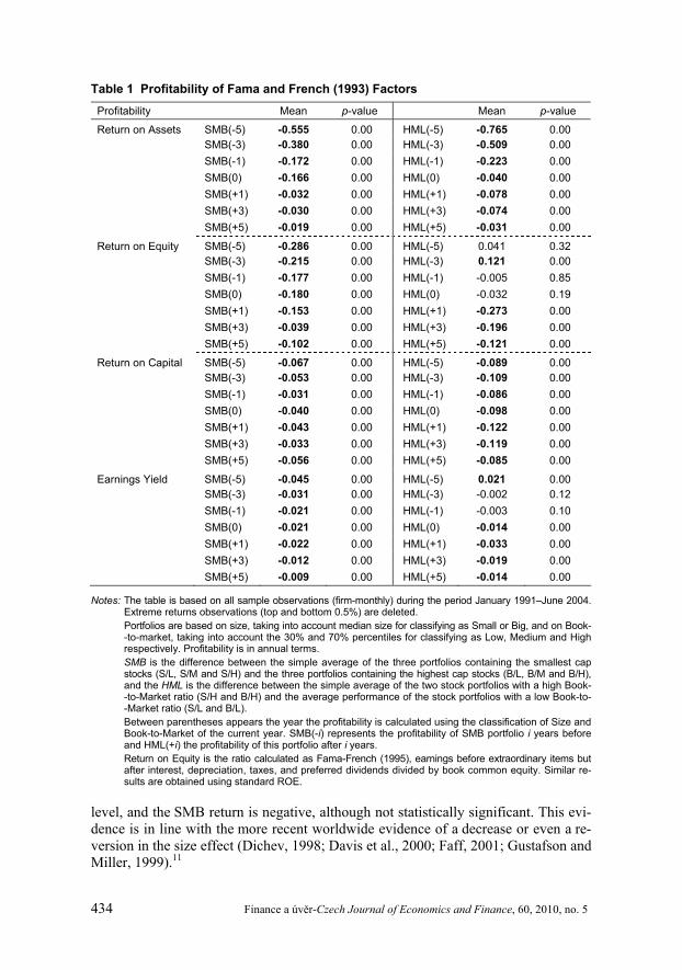
In this line, this work analyzes the persistence of FF (1993) factors based on profitability. Table 1 reports mean values of profitability for size and BM factors for 11 years around portfolio formation. As it can be seen as a global result, the persist-ence of size and BM factor is very high for all fundamental variables. Profitability is always significant after portfolio formation. It seems that there are factors in funda-mentals similar to factors in returns.

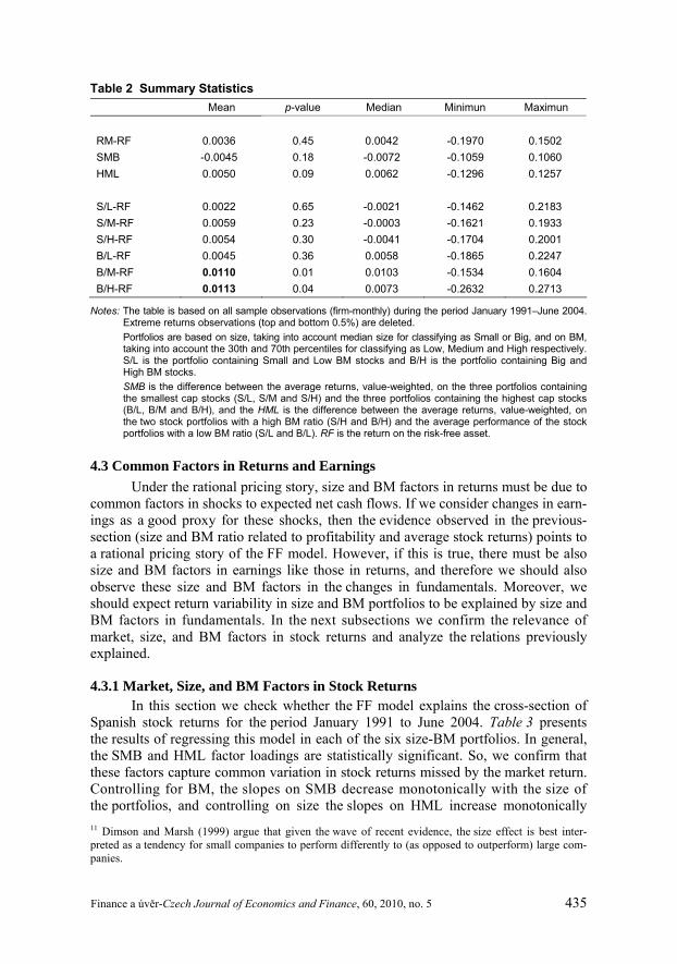
4.2 Descriptive Statistics Table 2 presents descriptive statistics of the portfolios’ monthly returns used

in this study. The results show that the worldwide evidence for a positive relation between BM ratio and returns holds. High BM stocks yield, on average, higher returns than low BM stocks regardless of the size level, and the HML return is positive, although only significant at the 10% level. Regarding the size effect, the re-sults show a positive, rather than the expected negative, relation between size and returns. Big stocks yield higher returns than small stocks independently of the BM


Table 1 Profitability of Fama and French (1993) Factors

Profitability Mean p-value Mean p-value

Return on Assets SMB(-5) -0.555 0.00 HML(-5) -0.765 0.00 SMB(-3) -0.380 0.00 HML(-3) -0.509 0.00 SMB(-1) -0.172 0.00 HML(-1) -0.223 0.00 SMB(0) -0.166 0.00 HML(0) -0.040 0.00 SMB(+1) -0.032 0.00 HML(+1) -0.078 0.00 SMB(+3) -0.030 0.00 HML(+3) -0.074 0.00 SMB(+5) -0.019 0.00 HML(+5) -0.031 0.00

Return on Equity SMB(-5) -0.286 0.00 HML(-5) 0.041 0.32 SMB(-3) -0.215 0.00 HML(-3) 0.121 0.00 SMB(-1) -0.177 0.00 HML(-1) -0.005 0.85 SMB(0) -0.180 0.00 HML(0) -0.032 0.19 SMB(+1) -0.153 0.00 HML(+1) -0.273 0.00 SMB(+3) -0.039 0.00 HML(+3) -0.196 0.00 SMB(+5) -0.102 0.00 HML(+5) -0.121 0.00

Return on Capital SMB(-5) -0.067 0.00 HML(-5) -0.089 0.00 SMB(-3) -0.053 0.00 HML(-3) -0.109 0.00 SMB(-1) -0.031 0.00 HML(-1) -0.086 0.00 SMB(0) -0.040 0.00 HML(0) -0.098 0.00 SMB(+1) -0.043 0.00 HML(+1) -0.122 0.00 SMB(+3) -0.033 0.00 HML(+3) -0.119 0.00 SMB(+5) -0.056 0.00 HML(+5) -0.085 0.00

Earnings Yield SMB(-5) -0.045 0.00 HML(-5) 0.021 0.00 SMB(-3) -0.031 0.00 HML(-3) -0.002 0.12 SMB(-1) -0.021 0.00 HML(-1) -0.003 0.10 SMB(0) -0.021 0.00 HML(0) -0.014 0.00 SMB(+1) -0.022 0.00 HML(+1) -0.033 0.00 SMB(+3) -0.012 0.00 HML(+3) -0.019 0.00 SMB(+5) -0.009 0.00 HML(+5) -0.014 0.00

Notes: The table is based on all sample observations (firm-monthly) during the period January 1991–June 2004. Extreme returns observations (top and bottom 0.5%) are deleted. Portfolios are based on size, taking into account median size for classifying as Small or Big, and on Book- -to-market, taking into account the 30% and 70% percentiles for classifying as Low, Medium and High respectively. Profitability is in annual terms. SMB is the difference between the simple average of the three portfolios containing the smallest cap stocks (S/L, S/M and S/H) and the three portfolios containing the highest cap stocks (B/L, B/M and B/H), and the HML is the difference between the simple average of the two stock portfolios with a high Book- -to-Market ratio (S/H and B/H) and the average performance of the stock portfolios with a low Book-to- -Market ratio (S/L and B/L). Between parentheses appears the year the profitability is calculated using the classification of Size and Book-to-Market of the current year. SMB(-i) represents the profitability of SMB portfolio i years before and HML(+i) the profitability of this portfolio after i years. Return on Equity is the ratio calculated as Fama-French (1995), earnings before extraordinary items but after interest, depreciation, taxes, and preferred dividends divided by book common equity. Similar re-sults are obtained using standard ROE.

level, and the SMB return is negative, although not statistically significant. This evi-dence is in line with the more recent worldwide evidence of a decrease or even a re-version in the size effect (Dichev, 1998; Davis et al., 2000; Faff, 2001; Gustafson and Miller, 1999).11


Table 2 Summary Statistics Mean p-value Median Minimun Maximun

RM-RF 0.0036 0.45 0.0042 -0.1970 0.1502 SMB -0.0045 0.18 -0.0072 -0.1059 0.1060 HML 0.0050 0.09 0.0062 -0.1296 0.1257

S/L-RF 0.0022 0.65 -0.0021 -0.1462 0.2183 S/M-RF 0.0059 0.23 -0.0003 -0.1621 0.1933 S/H-RF 0.0054 0.30 -0.0041 -0.1704 0.2001 B/L-RF 0.0045 0.36 0.0058 -0.1865 0.2247 B/M-RF 0.0110 0.01 0.0103 -0.1534 0.1604 B/H-RF 0.0113 0.04 0.0073 -0.2632 0.2713

Notes: The table is based on all sample observations (firm-monthly) during the period January 1991–June 2004. Extreme returns observations (top and bottom 0.5%) are deleted. Portfolios are based on size, taking into account median size for classifying as Small or Big, and on BM, taking into account the 30th and 70th percentiles for classifying as Low, Medium and High respectively. S/L is the portfolio containing Small and Low BM stocks and B/H is the portfolio containing Big and High BM stocks. SMB is the difference between the average returns, value-weighted, on the three portfolios containing the smallest cap stocks (S/L, S/M and S/H) and the three portfolios containing the highest cap stocks (B/L, B/M and B/H), and the HML is the difference between the average returns, value-weighted, on the two stock portfolios with a high BM ratio (S/H and B/H) and the average performance of the stock portfolios with a low BM ratio (S/L and B/L). RF is the return on the risk-free asset.

4.3 Common Factors in Returns and Earnings Under the rational pricing story, size and BM factors in returns must be due to

common factors in shocks to expected net cash flows. If we consider changes in earn-ings as a good proxy for these shocks, then the evidence observed in the previous-section (size and BM ratio related to profitability and average stock returns) points to a rational pricing story of the FF model. However, if this is true, there must be also size and BM factors in earnings like those in returns, and therefore we should also observe these size and BM factors in the changes in fundamentals. Moreover, we should expect return variability in size and BM portfolios to be explained by size and BM factors in fundamentals. In the next subsections we confirm the relevance of market, size, and BM factors in stock returns and analyze the relations previously explained.

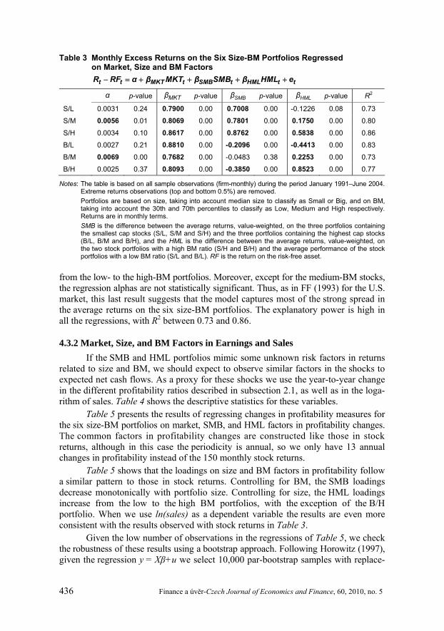
4.3.1 Market, Size, and BM Factors in Stock Returns In this section we check whether the FF model explains the cross-section of

Spanish stock returns for the period January 1991 to June 2004. Table 3 presents the results of regressing this model in each of the six size-BM portfolios. In general, the SMB and HML factor loadings are statistically significant. So, we confirm that these factors capture common variation in stock returns missed by the market return. Controlling for BM, the slopes on SMB decrease monotonically with the size of the portfolios, and controlling on size the slopes on HML increase monotonically 11 Dimson and Marsh (1999) argue that given the wave of recent evidence, the size effect is best inter-preted as a tendency for small companies to perform differently to (as opposed to outperform) large com-panies.


Table 3 Monthly Excess Returns on the Six Size-BM Portfolios Regressed on Market, Size and BM Factors

− = + + + +t t MKT t SMB t HML t tR RF α β MKT β SMB β HML e

α p-value MKTβ p-value SMBβ p-value HMLβ p-value R2

S/L 0.0031 0.24 0.7900 0.00 0.7008 0.00 -0.1226 0.08 0.73

S/M 0.0056 0.01 0.8069 0.00 0.7801 0.00 0.1750 0.00 0.80

S/H 0.0034 0.10 0.8617 0.00 0.8762 0.00 0.5838 0.00 0.86

B/L 0.0027 0.21 0.8810 0.00 -0.2096 0.00 -0.4413 0.00 0.83

B/M 0.0069 0.00 0.7682 0.00 -0.0483 0.38 0.2253 0.00 0.73

B/H 0.0025 0.37 0.8093 0.00 -0.3850 0.00 0.8523 0.00 0.77

Notes: The table is based on all sample observations (firm-monthly) during the period January 1991–June 2004. Extreme returns observations (top and bottom 0.5%) are removed. Portfolios are based on size, taking into account median size to classify as Small or Big, and on BM, taking into account the 30th and 70th percentiles to classify as Low, Medium and High respectively. Returns are in monthly terms. SMB is the difference between the average returns, value-weighted, on the three portfolios containing the smallest cap stocks (S/L, S/M and S/H) and the three portfolios containing the highest cap stocks (B/L, B/M and B/H), and the HML is the difference between the average returns, value-weighted, on the two stock portfolios with a high BM ratio (S/H and B/H) and the average performance of the stock portfolios with a low BM ratio (S/L and B/L). RF is the return on the risk-free asset.

from the low- to the high-BM portfolios. Moreover, except for the medium-BM stocks, the regression alphas are not statistically significant. Thus, as in FF (1993) for the U.S. market, this last result suggests that the model captures most of the strong spread in the average returns on the six size-BM portfolios. The explanatory power is high in all the regressions, with R2 between 0.73 and 0.86.

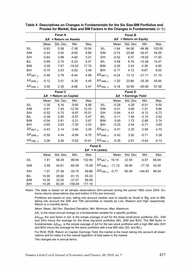
4.3.2 Market, Size, and BM Factors in Earnings and Sales If the SMB and HML portfolios mimic some unknown risk factors in returns

related to size and BM, we should expect to observe similar factors in the shocks to expected net cash flows. As a proxy for these shocks we use the year-to-year change in the different profitability ratios described in subsection 2.1, as well as in the loga-rithm of sales. Table 4 shows the descriptive statistics for these variables.

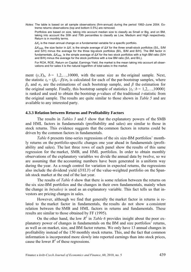
Table 5 presents the results of regressing changes in profitability measures for the six size-BM portfolios on market, SMB, and HML factors in profitability changes. The common factors in profitability changes are constructed like those in stock returns, although in this case the periodicity is annual, so we only have 13 annual changes in profitability instead of the 150 monthly stock returns.

Table 5 shows that the loadings on size and BM factors in profitability follow a similar pattern to those in stock returns. Controlling for BM, the SMB loadings decrease monotonically with portfolio size. Controlling for size, the HML loadings increase from the low to the high BM portfolios, with the exception of the B/H portfolio. When we use ln(sales) as a dependent variable the results are even more consistent with the results observed with stock returns in Table 3.

Given the low number of observations in the regressions of Table 5, we check the robustness of these results using a bootstrap approach. Following Horowitz (1997), given the regression y = Xβ+u we select 10,000 par-bootstrap samples with replace-


Table 4 Descriptives on Changes in Fundamentals for the Six Size-BM Portfolios and Proxies for Market, Size and BM Factors in the Changes in Fundamentals (in %)

Panel A ΔX = Return on Assets

Panel B ΔX = Return on Equity

Mean Std. Dev. Min Max Mean Std. Dev. Min Max S/L -0.63 5.08 -7.08 10.54 S/L -1.64 64.06 -94.98 103.05 S/M -0.44 5.55 -8.65 8.80 S/M -0.74 23.68 -30.47 54.29 S/H -0.64 2.68 -4.82 3.21 S/H -0.52 8.57 -16.63 17.50 B/L -0.69 2.70 -5.23 5.47 B/L 0.58 6.76 -10.26 14.47 B/M 0.05 7.67 -19.52 17.75 B/M 0.30 3.24 -5.38 6.90 B/H -0.70 2.53 -5.62 3.48 B/H -0.17 4.72 -9.67 8.02

,Δ MKT yX -0.46 2.78 -6.44 4.99 ,Δ MKT yX -0.24 13.12 -21.11 31.10

,Δ SMB yX -0.12 3.51 -9.30 4.40 ,Δ SMB yX -1.20 23.86 -35.39 45.94

,Δ HML yX 0.00 2.35 -4.66 3.47 ,Δ HML yX 0.18 32.59 -55.06 57.58

Panel C ΔX = Return on Capital

Panel D ΔX = Earnings Yield

Mean Std. Dev. Min Max Mean Std. Dev. Min Max S/L -1.30 6.16 -9.60 8.68 S/L -0.28 4.28 -6.51 9.50 S/M -0.91 7.44 -12.30 12.33 S/M -0.51 4.90 -7.51 9.86 S/H -0.52 4.75 -8.97 10.51 S/H -0.84 4.41 -9.13 6.73 B/L -0.39 2.80 -5.07 5.47 B/L -0.11 1.46 -3.15 2.62 B/M -0.04 2.61 -5.31 3.67 B/M 0.00 1.72 -2.68 3.74 B/H -0.65 2.63 -7.30 2.03 B/H -0.25 2.54 -5.71 3.85

,Δ MKT yX -0.43 2.14 -3.94 3.39 ,Δ MKT yX -0.31 2.20 -3.99 4.70

,Δ SMB yX -0.55 4.44 -8.99 6.75 ,Δ SMB yX -0.42 2.92 -5.71 5.38

,Δ HML yX 0.26 4.26 -5.52 10.41 ,Δ HML yX -0.35 2.91 -5.44 6.13

Panel E ΔX = ln (sales)

Mean Std. Dev. Min Max Mean Std. Dev. Min Max

S/L 1.81 58.29 -99.94 132.90 ,Δ MKT yX 19.14 22.50 -4.97 66.94

S/M 5.59 42.61 -82.49 75.08 ,Δ SMB yX -11.72 36.90 -77.78 42.50

S/H 1.01 27.36 -33.15 49.86 ,Δ HML yX -0.77 60.39 -144.93 86.54 B/L 15.00 29.82 -51.10 55.33 B/M 14.30 32.05 -37.57 89.58 B/H 14.26 83.20 -106.84 177.18

Notes: The table is based on all sample observations (firm-annual) during the period 1992–June 2004. Ex-treme returns observations (top and bottom 0.5%) are removed. Portfolios are based on size, taking into account median size to classify as Small or Big, and on BM, taking into account the 30th and 70th percentiles to classify as Low, Medium and High respectively. Return is in monthly terms. Mean: Mean; Std Dev: Standard Deviation; Min: Minimum; Max: Maximum. ΔXy is the mean annual change on a fundamental variable for a specific portfolio. ΔXSMB, the size factor in ΔX, is the simple average of ΔX for the three small-stock portfolios (S/L, S/M and S/H) minus the average for the three big-stock portfolios (B/L, B/M and B/H). The BM factor in fundamentals, ΔXHML, is the simple average of ΔX for the two stock portfolios with a high BM ratio (S/H and B/H) minus the average for the stock portfolios with a low BM ratio (S/L and B/L). For ROA, ROE, Return on Capital, Earnings Yield, the market is the mean taking into account all obser-vations and for sales it is the natural logarithm of total sales in the market. The changes are in annual terms.


Table 5 Changes in Fundamentals for the Six Size-BM Portfolios Regressed on Proxies for Market, Size and BM Factors in the Changes in Fundamentals

0 , , ,Δ Δ Δ Δ MKT MKT y SMB SMB y HML HML y yyX λ λ X λ X λ X e= + + + +

Panel A: ΔX = Return on Assets

β0 p-value β1 p-value β2 p-value β3 p-value R2 S/L -0.0035 0.62 0.5736 0.11 0.2419 0.27 -1.3592 0.01 0.83 S/M 0.0038 0.69 1.5445 0.01 0.8081 0.02 0.4844 0.38 0.74 S/H -0.0028 0.61 0.6368 0.03 0.4887 0.01 0.5127 0.13 0.63 B/L -0.0049 0.46 0.4017 0.21 0.1263 0.53 -0.3436 0.37 0.48 B/M 0.0081 0.45 2.0146 0.00 -1.4672 0.00 0.1971 0.74 0.84 B/H -0.0056 0.45 0.3386 0.34 -0.1204 0.59 -0.2155 0.61 0.27

Panel B: ΔX = Return on Equity

β0 p-value β1 p-value β2 p-value β3 p-value R2

S/L 0.0017 0.92 -1.0674 0.02 1.5249 0.00 -1.2509 0.00 0.99 S/M -0.0060 0.80 3.0254 0.00 -0.4406 0.42 0.3605 0.17 0.91 S/H 0.0066 0.71 -0.5729 0.21 1.1996 0.01 0.6414 0.01 0.61 B/L 0.0006 0.95 0.9403 0.00 -0.6618 0.02 -0.2827 0.02 0.79 B/M 0.0060 0.43 -0.0012 0.99 0.2822 0.12 0.2088 0.02 0.52 B/H -0.0044 0.68 0.4459 0.11 -0.3365 0.18 -0.1750 0.13 0.55

Panel C: ΔX = Return on Capital

β0 p-value β1 p-value β2 p-value β3 p-value R2 S/L -0.0045 0.63 0.8342 0.21 0.5108 0.10 -0.8363 0.01 0.80 S/M 0.0002 0.98 1.1291 0.22 1.0286 0.03 0.4581 0.21 0.74 S/H -0.0003 0.97 0.9971 0.06 0.4518 0.06 0.7001 0.00 0.81 B/L -0.0014 0.76 1.0006 0.01 -0.4424 0.01 -0.2427 0.07 0.77 B/M 0.0025 0.68 1.1220 0.02 -0.1830 0.35 0.3436 0.07 0.51 B/H -0.0056 0.46 0.8378 0.13 -0.3834 0.13 0.2210 0.30 0.27

Panel D: ΔX = Earnings Yield


S/L -0.0006 0.94 0.5382 0.49 0.7786 0.20 -0.7837 0.01 0.75 S/M 0.0005 0.90 2.7599 0.00 -0.5241 0.18 -0.2182 0.20 0.93 S/H -0.0011 0.57 -0.3950 0.08 1.3232 0.00 0.8476 0.00 0.98 B/L -0.0017 0.48 0.4936 0.08 -0.1872 0.36 -0.3867 0.00 0.76 B/M 0.0018 0.65 0.9826 0.04 -0.5032 0.15 0.2504 0.11 0.53 B/H -0.0012 0.86 1.4269 0.08 -0.7319 0.21 -0.0180 0.94 0.36

Panel E: ΔX = ln (sales)


S/L -0.0030 0.99 0.6022 0.35 0.8182 0.14 -0.2209 0.49 0.52 S/M -0.1010 0.49 1.1489 0.04 0.5289 0.22 0.1329 0.60 0.43 S/H 0.1334 0.15 -0.2989 0.34 0.5405 0.05 0.3595 0.04 0.49 B/L 0.0227 0.79 0.2081 0.49 -0.7170 0.01 -0.4555 0.01 0.59 B/M 0.1205 0.35 0.1348 0.76 0.0438 0.90 -0.2373 0.29 0.25 B/H -0.1138 0.52 1.1092 0.09 -0.4393 0.39 0.9642 0.01 0.79


Notes: The table is based on all sample observations (firm-annual) during the period 1992–June 2004. Ex-treme returns observations (top and bottom 0.5%) are removed. Portfolios are based on size, taking into account median size to classify as Small or Big, and on BM, taking into account the 30th and 70th percentiles to classify as Low, Medium and High respectively. Return is in monthly terms. ΔXy is the mean annual change on a fundamental variable for a specific portfolio. ΔXSMB, the size factor in ΔX, is the simple average of ΔX for the three small-stock portfolios (S/L, S/M and S/H) minus the average for the three big-stock portfolios (B/L, B/M and B/H). The BM factor in fundamentals, ΔXHML, is the simple average of ΔX for the two stock portfolios with a high BM ratio (S/H and B/H) minus the average for the stock portfolios with a low BM ratio (S/L and B/L). For ROA, ROE, Return on Capital, Earnings Yield, the market is the mean taking into account all obser-vations and for sales it is the natural logarithm of total sales in the market.

ment (y,X)b, b = 1,2,…,10000, with the same size as the original sample. Next, the statistic tb = (βb – β)/σb is calculated for each of the par-bootstrap samples, where βb and σb are the estimations of each bootstrap sample, and β the estimation for the original sample. Finally, this bootstrap sample of statistics {tb : b = 1,2,…,10000} is ranked and used to obtain the bootstrap p-values of the traditional t-statistic from the original sample. The results are quite similar to those shown in Table 5 and are available to any interested party.

4.3.3 Relation between Returns and Profitability Factors The results in Tables 3 and 5 show that the explanatory powers of the SMB

and HML factors in fundamentals (profitability and sales) are similar to those in stock returns. This evidence suggests that the common factors in returns could be driven by the common factors in fundamentals.

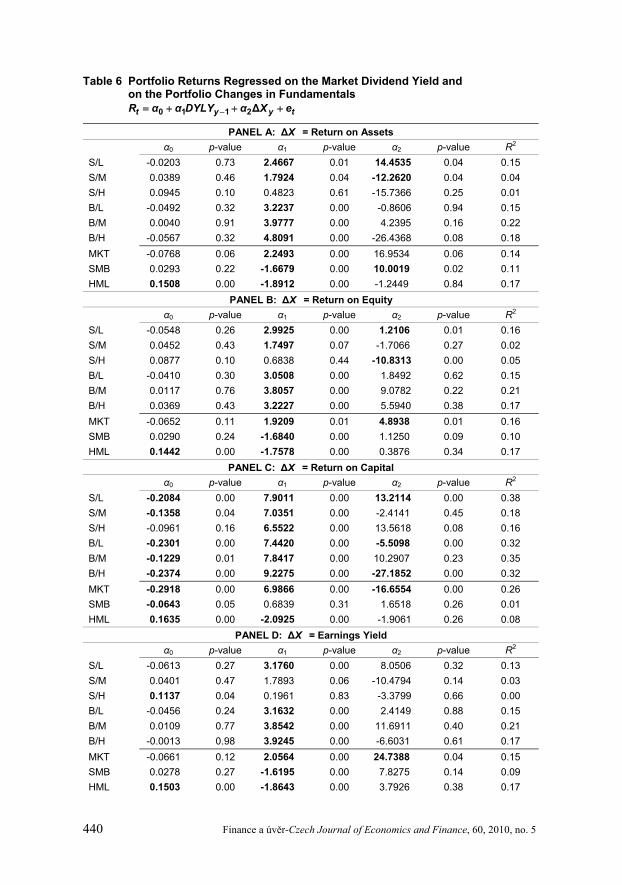
Table 6 presents time-series regressions of the six size-BM portfolios’ month-ly returns on the portfolio-specific changes one year ahead in fundamentals (profit-ability and sales). The last three rows of each panel show the results of this same regression for the market, SMB, and HML portfolios. In order to obtain monthly observations of the explanatory variables we divide the annual data by twelve, so we are assuming that the accounting numbers have been generated in a uniform way during the year. As a rough control for variation in expected returns, the regressions also include the dividend yield (DYLY) of the value-weighted portfolio on the Span-ish stock market at the end of the last year.

The results of Table 6 show that there is some relation between the returns on the six size-BM portfolios and the changes in their own fundamentals, mainly when the change in ln(sales) is used as an explanatory variable. This fact tells us that in-vestors are pricing changes in sales.

However, although we find that generally the market factor in returns is re-lated to the market factor in fundamentals, the results do not show a consistent relation between the SMB and HML factors in returns and fundamentals. These results are similar to those obtained by FF (1995).

On the other hand, the low R2 in Table 6 provides insight about the poor ex-planatory power of changes in fundamentals on the BM and size portfolios’ returns, as well as on market, size, and BM factor returns. We only have 13 annual changes in profitability instead of the 150 monthly stock returns. This, and the fact that common information is incorporated more slowly into reported earnings than into stock prices, cause the lower R2 of these regressions.


Table 6 Portfolio Returns Regressed on the Market Dividend Yield and on the Portfolio Changes in Fundamentals

−= + + +0 1 1 2Δt y y tR α α DYLY α X e

PANEL A: ΔX = Return on Assets α0 p-value α1 p-value α2 p-value R2 S/L -0.0203 0.73 2.4667 0.01 14.4535 0.04 0.15 S/M 0.0389 0.46 1.7924 0.04 -12.2620 0.04 0.04 S/H 0.0945 0.10 0.4823 0.61 -15.7366 0.25 0.01 B/L -0.0492 0.32 3.2237 0.00 -0.8606 0.94 0.15 B/M 0.0040 0.91 3.9777 0.00 4.2395 0.16 0.22 B/H -0.0567 0.32 4.8091 0.00 -26.4368 0.08 0.18 MKT -0.0768 0.06 2.2493 0.00 16.9534 0.06 0.14 SMB 0.0293 0.22 -1.6679 0.00 10.0019 0.02 0.11 HML 0.1508 0.00 -1.8912 0.00 -1.2449 0.84 0.17

PANEL B: ΔX = Return on Equity α0 p-value α1 p-value α2 p-value R2 S/L -0.0548 0.26 2.9925 0.00 1.2106 0.01 0.16 S/M 0.0452 0.43 1.7497 0.07 -1.7066 0.27 0.02 S/H 0.0877 0.10 0.6838 0.44 -10.8313 0.00 0.05 B/L -0.0410 0.30 3.0508 0.00 1.8492 0.62 0.15 B/M 0.0117 0.76 3.8057 0.00 9.0782 0.22 0.21 B/H 0.0369 0.43 3.2227 0.00 5.5940 0.38 0.17 MKT -0.0652 0.11 1.9209 0.01 4.8938 0.01 0.16 SMB 0.0290 0.24 -1.6840 0.00 1.1250 0.09 0.10 HML 0.1442 0.00 -1.7578 0.00 0.3876 0.34 0.17

PANEL C: ΔX = Return on Capital α0 p-value α1 p-value α2 p-value R2 S/L -0.2084 0.00 7.9011 0.00 13.2114 0.00 0.38 S/M -0.1358 0.04 7.0351 0.00 -2.4141 0.45 0.18 S/H -0.0961 0.16 6.5522 0.00 13.5618 0.08 0.16 B/L -0.2301 0.00 7.4420 0.00 -5.5098 0.00 0.32 B/M -0.1229 0.01 7.8417 0.00 10.2907 0.23 0.35 B/H -0.2374 0.00 9.2275 0.00 -27.1852 0.00 0.32 MKT -0.2918 0.00 6.9866 0.00 -16.6554 0.00 0.26 SMB -0.0643 0.05 0.6839 0.31 1.6518 0.26 0.01 HML 0.1635 0.00 -2.0925 0.00 -1.9061 0.26 0.08

PANEL D: ΔX = Earnings Yield α0 p-value α1 p-value α2 p-value R2 S/L -0.0613 0.27 3.1760 0.00 8.0506 0.32 0.13 S/M 0.0401 0.47 1.7893 0.06 -10.4794 0.14 0.03 S/H 0.1137 0.04 0.1961 0.83 -3.3799 0.66 0.00 B/L -0.0456 0.24 3.1632 0.00 2.4149 0.88 0.15 B/M 0.0109 0.77 3.8542 0.00 11.6911 0.40 0.21 B/H -0.0013 0.98 3.9245 0.00 -6.6031 0.61 0.17 MKT -0.0661 0.12 2.0564 0.00 24.7388 0.04 0.15 SMB 0.0278 0.27 -1.6195 0.00 7.8275 0.14 0.09 HML 0.1503 0.00 -1.8643 0.00 3.7926 0.38 0.17


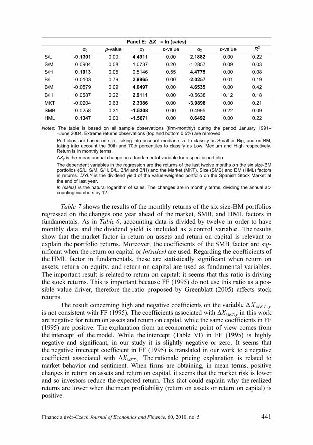
Panel E: ΔX = ln (sales) α0 p-value α1 p-value α2 p-value R2 S/L -0.1301 0.00 4.4911 0.00 2.1882 0.00 0.22 S/M 0.0904 0.08 1.0737 0.20 -1.2857 0.09 0.03 S/H 0.1013 0.05 0.5146 0.55 4.4775 0.00 0.08 B/L -0.0103 0.79 2.9965 0.00 -2.0257 0.01 0.19 B/M -0.0579 0.09 4.0497 0.00 4.6535 0.00 0.42 B/H 0.0587 0.22 2.9111 0.00 -0.5638 0.12 0.18 MKT -0.0204 0.63 2.3386 0.00 -3.9898 0.00 0.21 SMB 0.0258 0.31 -1.5308 0.00 0.4995 0.22 0.09 HML 0.1347 0.00 -1.5671 0.00 0.6492 0.00 0.22

Notes: The table is based on all sample observations (firm-monthly) during the period January 1991– –June 2004. Extreme returns observations (top and bottom 0.5%) are removed. Portfolios are based on size, taking into account median size to classify as Small or Big, and on BM, taking into account the 30th and 70th percentiles to classify as Low, Medium and High respectively. Return is in monthly terms. ΔXy is the mean annual change on a fundamental variable for a specific portfolio. The dependent variables in the regression are the returns of the last twelve months on the six size-BM portfolios (S/L, S/M, S/H, B/L, B/M and B/H) and the Market (MKT), Size (SMB) and BM (HML) factors in returns. DYLY is the dividend yield of the value-weighted portfolio on the Spanish Stock Market at the end of last year. ln (sales) is the natural logarithm of sales. The changes are in monthly terms, dividing the annual ac-counting numbers by 12.

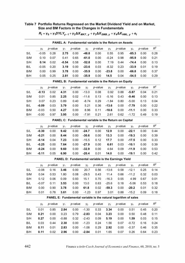
Table 7 shows the results of the monthly returns of the six size-BM portfolios

regressed on the changes one year ahead of the market, SMB, and HML factors in fundamentals. As in Table 6, accounting data is divided by twelve in order to have monthly data and the dividend yield is included as a control variable. The results show that the market factor in return on assets and return on capital is relevant to explain the portfolio returns. Moreover, the coefficients of the SMB factor are sig-nificant when the return on capital or ln(sales) are used. Regarding the coefficients of the HML factor in fundamentals, these are statistically significant when return on assets, return on equity, and return on capital are used as fundamental variables. The important result is related to return on capital: it seems that this ratio is driving the stock returns. This is important because FF (1995) do not use this ratio as a pos-sible value driver, therefore the ratio proposed by Greenblatt (2005) affects stock returns.

The result concerning high and negative coefficients on the variable ΔX M K T , y is not consistent with FF (1995). The coefficients associated with ΔXMKT,y in this work are negative for return on assets and return on capital, while the same coefficients in FF (1995) are positive. The explanation from an econometric point of view comes from the intercept of the model. While the intercept (Table VI) in FF (1995) is highly negative and significant, in our study it is slightly negative or zero. It seems that the negative intercept coefficient in FF (1995) is translated in our work to a negative coefficient associated with ΔXMKT,y. The rationale pricing explanation is related to market behavior and sentiment. When firms are obtaining, in mean terms, positive changes in return on assets and return on capital, it seems that the market risk is lower and so investors reduce the expected return. This fact could explain why the realized returns are lower when the mean profitability (return on assets or return on capital) is positive.


Table 7 Portfolio Returns Regressed on the Market Dividend Yield and on Market, Size and BM Factors in the Changes in Fundamentals

−= + + + + +0 1 1 2 , 3 , 4 ,Δ Δ Δt y MKT y SMB y HML y tR γ γ DYLY γ X γ X γ X e

PANEL A: Fundamental variable is the Return on Assets

γ0 p-value γ1 p-value γ2 p-value γ3 p-value γ4 p-value R2 S/L -0.05 0.28 2.75 0.00 -48.8 0.00 0.55 0.95 -85.3 0.00 0.28 S/M 0.10 0.07 0.41 0.65 -61.0 0.00 -0.24 0.98 -95.9 0.00 0.21 S/H 0.14 0.02 -0.54 0.58 -52.8 0.00 7.19 0.44 -74.4 0.00 0.13 B/L -0.05 0.20 3.19 0.00 -23.6 0.03 -8.32 0.23 -33.9 0.01 0.19 B/M 0.00 0.99 3.78 0.00 -35.9 0.00 -23.8 0.00 -66.8 0.00 0.37 B/H 0.05 0.25 2.81 0.00 -35.9 0.00 14.5 0.04 -54.5 0.00 0.29

PANEL B: Fundamental variable is the Return on Equity

γ0 p-value γ1 p-value γ2 p-value γ3 p-value γ4 p-value R2 S/L -0.13 0.02 4.31 0.00 -13.0 0.08 0.92 0.88 -5.87 0.04 0.21 S/M 0.01 0.85 2.25 0.02 -11.6 0.13 -5.16 0.43 -9.46 0.00 0.13 S/H 0.07 0.23 0.89 0.40 -8.74 0.29 -1.84 0.80 -5.00 0.13 0.04 B/L -0.09 0.03 3.79 0.00 5.21 0.36 -13.6 0.00 -7.79 0.00 0.22 B/M -0.03 0.50 4.27 0.00 8.96 0.11 -18.6 0.00 -11.1 0.00 0.33 B/H -0.00 0.97 3.95 0.00 -7.91 0.21 2.61 0.62 -1.72 0.49 0.19

PANEL C: Fundamental variable is the Return on Capital

γ0 p-value γ1 p-value γ2 p-value γ3 p-value γ4 p-value R2 S/L -0.30 0.00 9.42 0.00 -24.7 0.00 12.9 0.00 -22.1 0.00 0.44 S/M -0.21 0.00 8.44 0.00 -30.6 0.00 13.3 0.00 -19.3 0.00 0.39 S/H -0.14 0.04 7.23 0.00 -15.5 0.12 17.7 0.00 -17.5 0.00 0.33 B/L -0.25 0.00 7.64 0.00 -27.9 0.00 6.61 0.03 -10.1 0.00 0.39 B/M -0.24 0.00 9.60 0.00 -32.9 0.00 4.64 0.09 -11.9 0.00 0.53 B/H -0.11 0.05 6.90 0.00 -20.4 0.01 14.0 0.00 -19.1 0.00 0.42

PANEL D: Fundamental variable is the Earnings Yield

γ0 p-value γ1 p-value γ2 p-value γ3 p-value γ4 p-value R2 S/L -0.08 0.16 3.46 0.00 20.7 0.56 -13.6 0.58 -12.1 0.25 0.14 S/M 0.04 0.53 1.80 0.08 -29.5 0.43 11.4 0.66 -11.2 0.32 0.03 S/H 0.12 0.06 0.09 0.93 15.1 0.70 -16.3 0.55 4.99 0.67 0.01 B/L -0.07 0.11 3.53 0.00 13.0 0.63 -25.6 0.18 -5.06 0.53 0.18 B/M 0.00 0.90 3.78 0.00 61.8 0.02 -59.3 0.00 -20.2 0.01 0.32 B/H 0.01 0.78 3.61 0.00 -1.23 0.97 3.01 0.88 -15.2 0.09 0.18

PANEL E: Fundamental variable is the natural logarithm of sales

γ0 p-value γ1 p-value γ2 p-value γ3 p-value γ4 p-value R2

S/L 0.01 0.85 2.84 0.00 -1.30 0.33 3.34 0.00 0.51 0.45 0.20 S/M 0.21 0.00 0.23 0.79 -2.83 0.04 3.23 0.00 0.50 0.48 0.11 S/H 0.27 0.00 -0.88 0.32 -2.43 0.09 5.19 0.00 1.59 0.03 0.15 B/L 0.03 0.44 2.30 0.00 -1.23 0.24 1.56 0.07 -0.72 0.16 0.24 B/M 0.11 0.01 2.83 0.00 -1.08 0.29 2.92 0.00 -0.37 0.46 0.35 B/H 0.11 0.02 2.96 0.00 -2.84 0.01 1.65 0.07 0.26 0.64 0.23


Notes: The table is based on all sample observations (firm-monthly) during the period January 1991–June 2004. Extreme returns observations (top and bottom 0.5%) are removed. Portfolios are based on size, taking into account median size to classify as Small or Big, and on BM, taking into account the 30th and 70th percentiles to classify as Low, Medium and High respectively. Return is in monthly terms. Δ SMBX , the size factor in the fundamental variable, is the simple average of the fundamental variable

for the three small-stock portfolios (S/L, S/M and S/H) minus the average for the three big-stock port-folios (B/L, B/M and B/H). The BM factor, Δ HMLX , is the simple average of the fundamental variable for the two stock portfolios with a high BM ratio (S/H and B/H) minus the average for the stock portfolios with a low BM ratio (S/L and B/L). DYLY is the dividend yield of the value-weighted portfolio on the Spanish Stock Market at the end of last year, ln (sales) is the natural logarithm of sales. For ROA, ROE, Return on Capital, Earnings Yield, the market is the mean taking into account all ob-servations and for sales it is the natural logarithm of total sales in the market. The changes are in monthly terms, dividing the annual accounting numbers by 12.

In brief, the results of Table 6 show that changes in sales are captured by in-

vestors, and the results of Table 7 report that return on capital could be driving stock returns on the Spanish stock market. Therefore, there is a relation between factors in fundamentals and factors in returns, and this fact gives support to the use of the FF (1993) model in this market.

However, the evidence is somewhat weaker for the other fundamental vari-ables. These results have some similarity to those obtained by FF (1995). As they suggest, the low observation frequency of the accounting data and the smooth incor-poration of shocks in expected future cash flows in the accounting data makes it very difficult to have good measures of shocks to fundamentals and therefore good meas-ures of the links between stock returns and the common factors in fundamentals.

5. Conclusions Since the publication of the Fama and French (1993) model, the three-factor

model has become highly popular among academics and practitioners at international level. However, there exists in the finance literature considerable controversy regard-ing whether the SMB and HML factors are real proxies for risk factors or not, be-cause CAPM has been built from microfoundations but the FF model is derived purely from an empirical standpoint. This question has inspired a number of studies in the U.S. market which try to give rational support to this model, but there is little evidence concerning this problem in non-U.S. markets. It seems reasonable to as-sume that, before applying this model in other countries, it is necessary to evaluate whether the factors are proxying for risk in other countries or not. However, this model has been applied in a considerable number of different countries without this concern being checked.

The goal of our study is to provide evidence in favor of a rationale expla-nation of the good performance of this model in the Spanish market. Following the approach of FF (1995), we demonstrate that there are SMB and HML factors in fundamentals similar to those observed in returns. Moreover, we find that return on capital is a useful fundamental variable used by investors in the Spanish stock mar-ket, so that when this ratio is used as a proxy for fundamentals, SMB and HML fac-tors in fundamentals not only are similar to factors in returns, but also drive factors in returns. Of course, this evidence is more consistent with a rationale explanation than a spurious or mispricing explanation of this model.


We believe that our results offer an important contribution. Our evidence gives support to the use, in a non-U.S. market, of the FF factors as proxies for risk factors and therefore indicates that this model is a good approach with which to achieve better estimates of expected returns. Moreover, our evidence offers out-of-sample evidence of the results observed by FF (1995) in the U.S. market. Of course, it would be interesting to extend this study to other European countries.

REFERENCES

Amihud Y, Christensen B, Mendelson H (1993): Further evidence on the risk-return relationship. Unpublished manuscript. Berk J (1995): A critique of size-related anomalies. Review of Financial Studies, 8:275–286.

Berk J, Green RC, Naik V (1999): Optimal investment, growth options, and security returns. Journal of Finance, 54:1553–1608.

Bhardwaj R, Brooks L (1993): Dual betas from bull and bear markets: reversal of the size effect. Journal of Financial Research, 16:269–83. Brennan MJ, Wang AW, Xia Y (2001): Intertemporal Capital Asset Pricing and the Fama-French Three-Factor Model. University of Pennsylvania Working Paper.

Cai J (1997): Glamour and value strategies on the Toyo stock exchange. Journal of Business Finance and Accounting, 24(9, 10): 0306–686X.

Cao Q, Leggio KB, Schniederjans MJ (2005): A comparison between Fama and French’s model and artificial neural networks in predicting the Chinese stock market. Computers and Operations Research, 32:2499–2512. Chan L, Hamao Y, Lakonishok J (1991): Fundamentals and stock returns in Japan. Journal of Finance, 46:1739–1789. Chang RP, McLeavy DW, Rhree SG (1995): Short-term abnormal returns of the contrarian strategy in the Japanese stock market. Journal of Business Finance and Accounting, 22(7):0306-686X. Charitou A, Constantinidis E (2004): Size and Book-to-Market Factors in Earnings and Stock Returns: Empirical Evidence for Japan. Working paper, University of Cyprus.

Chui ACW, Wei KCJ (1998): Book-to-market, firm size, and the turn-of-the-year effect: Evidence from Pacific-Basin emerging markets. Pacific-Basin Finance Journal, 6:275–293.

Daniel K, Titman S (1997): Evidence on the characteristics of cross-sectional variation in stock returns. Journal of Finance, 52:1–33.

Daniel K, Titman S, Wei KCJ (2001): Explaining the cross-section of stock returns in Japan: factors or characteristics? Journal of Finance, 56:743–766.

Davis J, Fama EF, French KR (2000): Characteristics, covariances, and average returns: 1929–1997. Journal of Finance, 55:389–406.

Dichev I (1998): Is the risk of bankruptcy a systematic risk? Journal of Finance, 56:1131–1147.

Dimson E, Marsh P (1999): Murphy's Law and Market Anomalies. Journal of Portfolio Man-agement, 25(2):53–69. Faff R (2001): An examination of the Fama and French three-factor model using commercially available factors. Australian Journal of Management, 26:1–17. Faff R (2004): A simple test of the Fama and French model using daily data: Australian evidence. Applied Financial Economics, 14:83–92. Fama EF, French K (1992): The cross-section of expected stock returns. Journal of Finance, 47: 427–465.


Fama EF, French K (1993): Common Risk Factors in the Returns on Stocks and Bonds. Journal of Financial Economics, 33:3–56. Fama EF, French K (1995): Size and Book-to-Market Factors in Earnings and Returns. Journal of Finance, 50(1):131–155. Fama EF, French K (1996): Multifactor explanations of asset pricing anomalies. Journal of Finance, 51:55–84. Fama EF, French K (1998): Value versus Growth: The International Evidence. Journal of Finance, 53:1975–1999. Ferson WE, Sarkissian S, Simin TR (1999): The Alpha Factor Asset Pricing Model: A Parable. Journal of Financial Markets, 2:49–68. Forner C, Marhuenda J (2006): Análisis del origen de los beneficios del momentum en el mercado de valores español. Investigaciones Económicas, 30(3):401–439. Forner C, Sanabria S, Marhuenda J (2009): Post-earnings announcement drift: Spanish evidence. Spanish Economic Review, 11(3):207–241. Gaunt C (2004): Size and book to market effects and the Fama and French three factor asset pricing model: evidence from the Australian stock market. Accounting and Finance, 44:27–44. Gomes J, Kogan L, Zhang L (2003): Equilibrium cross-section of returns. Journal of Political Economy, 111:693–732. Gómez-Biscarri J, López-Espinosa G (2008): Accounting Measures and International Pricing Models: Justifying Accounting Homogeneity. Journal of Accounting and Public Policy, 27:339–354. Gregory A, Harris R, Michou M (2003): Contrarian investment and macroeconomic risk. Journal of Business Finance and Accounting, 30(1, 2):0306–686X. Greenblatt J (2005): The little book that beats the market. John Wiley & Sons Inc. Griffin JM (2002): Are the Fama and French Factors Global or Country Specific? Review of Finan-cial Studies, 15:783–803. Grundy B, Malkiel B (1996): Reports of betas death have been greatly exaggerated. Journal of Portfolio Management, Spring, pp. 36–44.

Gustafson K, Miller J (1999): Where has the small-stock premium gone? Journal of Investing, 8:45–53.

Hahn J, Lee H (2006): Yield spreads as alternative risk factors for size and book-to-market. Journal of Financial and Quantitative Analysis, 41:245–69.

Horowitz JL (1997): Bootstrap methods in econometrics: Theory and numerical performance. In: Kreps DM, Wallis KF (Eds.): Advances in Economics and Econometrics: Theory and Applications, Seventh World Congress. Cambridge, Cambridge University Press.

Howton S, Peterson D (1998): An examination of crosssectional realized stock returns using a varying-risk beta model. Financial Review, 33:199–212. Jagannathan R, Wang Z (1996): The conditional CAPM and the cross-section of expected returns. Journal of Finance, 51:3–53. Kelly PJ (2003): Real and Inflationary Macroeconomic Risk in the Fama and French Size and Book- -to-Market Portfolios. EFMA 2003 Helsinki Meetings.

Lakonishok J, Shleifer A, Vishny R (1994): Contrarian investment, extrapolation, and risk. Journal of Finance, 49:1541–1578. Lawrencea E, Geppertb J, Prakasha A (2007): Asset pricing models: a comparison. Applied Finan-cial Economics, 17:933–940. Liew J, Vassalou M (2000): Can book-to-market, size and momentum be risk factors that predict economic growth? Journal of Financial Economics, 57:221–245.

Loughran T (1997): Book-to-market across firm size, exchange, and seasonality: is there an effect? Journal of Financial and Quantitative Analysis, 32:249–268.


Malin M, Veeraraghavan M (2004): On the robustness of the Fama and French multifactor model: evidence from France, Germany and the United Kingdom? International Journal of Business and Economics, 3:155–176. Malin M, Veeraraghavan M (2006): Firm size, beta and stock returns: evidence from Germany and the United Kingdom. International Economics and Finance Journal, 1(1):107–123. Matallín JC (2005): Portfolio Performance: Factors or Benchmarks? Available at SSRN: http://ssrn.com/abstract=760204. Merton RC (1973): An intertemporal capital asset pricing model. Econometrica, 41:867–887. Moerman GA (2005): How domestic is the Fama-French three factor model? An application to the Euro Area. ERIM Report Series Reference, no. ERS-2005-035-F&A. Moranaa C, Beltratti A (2006): Structural breaks and common factors in the volatility of the Fama- -French factor portfolios. Applied Financial Economics, 16:1059–1073. Myers SC (1984): The capital structure puzzle. Journal of Finance, 39:575–592. Nartea GV, Gan C, Wu J (2008): Persistence of size and value premia nad the robustness of the Fama-French Three Factor Model in the Hong Kong Stock Market. Investment Management and Financial Innovations, 5:9–49. Nieto B, Rodríguez R (2005): Modelos de valoración de activos condicionales: Un panorama com-parativo. Investigaciones económicas, 29:33–71. Pettengill G, Sundaram S, Mathur I (1995): The conditional relation between beta and returns. Journal of Financial and Quantitative Analysis, 30:101–16. Reverte C (2009): Do better governed firms enjoy a lower cost of equity capital? Evidence from Spanish firms. Corporate Governance, 9(2):133–145. Ross SA (1976): The arbitrage theory of capital asset pricing. Journal of Economic Theory, 13:341– –360. Simpson M, Ramchander S (2008): An inquiry into the economic fundamentals of the Fama and French equity factors. Journal of Empirical Finance, 15:801–815. Vassalou M (2003): News related to future GDP growth as a risk factor in equity returns. Journal of Financial Economics, 68(1):47–73. Vassalou M, Xing Y(2004): Default risk in equity returns. Journal of Finance, 59:831–868.

fundamentals and the origin of fama-french factors: the...

Documents