fundamental matrix computation: theory and …kanatani/papers/okafund.pdfsolution that satisﬁes...

Memoirs of the Faculty of Engineering, Okayama University, Vol. 42, pp. 18–35, January 2008

Fundamental Matrix Computation: Theory and Practice

Kenichi KANATANI∗ Yasuyuki SUGAYADepartment of Computer Science Department of Information and Computer Sciences

Okayama University Toyohashi University of TechnologyOkayama 700-8530 Japan Toyohashi, Aichi 441-8580 Japan

(Received November 14, 2007)

We classify and review existing algorithms for computing the fundamental matrix from pointcorrespondences and propose new effective schemes: 7-parameter Levenberg-Marquardt (LM)search, EFNS, and EFNS-based bundle adjustment. Doing experimental comparison, we showthat EFNS and the 7-parameter LM search exhibit the best performance and that additionalbundle adjustment does not increase the accuracy to any noticeable degree.

1. Introduction

Computing the fundamental matrix from pointcorrespondences is the first step of many vision appli-cations including camera calibration, image rectifica-tion, structure from motion, and new view generation[7]. Fundamental matrix computation has attracteda special attention because of the following two char-acteristics:

1. Feature points are extracted by an image pro-cessing operation [8, 17, 20, 23]. As a result, thedetected locations invariably have uncertainty tosome degree.

2. Detected points are matched by comparing sur-rounding regions in respective images, usingvarious measures of similarity and correlation[15, 19, 27]. However, mismatches are unavoid-able to some degree.

The first issue has been dealt with by statistical op-timization [10]: we model the uncertainty as “noise”obeying a certain probability distribution and com-pute a fundamental matrix such that its deviationfrom the true value is as small as possible in expecta-tion. The second issue has been coped with by robustestimation [21], which can be viewed as hypothesistesting: we compute a tentative fundamental matrixas a hypothesis and check how many points supportit. Those points regarded as “abnormal” according tothe hypothesis are called outliers, otherwise inliers,and we look for a fundamental matrix that has asmany inliers as possible.

———————This work is subjected to copyright.

All rights are reserved by this author/authors.

Thus, the two issues are inseparably interwoven.In this paper, we focus on the first issue, assumingthat all corresponding points are inliers. Such a study

∗E-mail [email protected]

is indispensable for any robust estimation techniqueto work successfully. However, there is an additionalcomplication in doing statistical optimization of thefundamental matrix: it is constrained to have rank2, i.e., its determinant is 0. This rank constraint hasbeen incorporated in various ways. Here, we catego-rize them into the following three approaches:

A posteriori correction

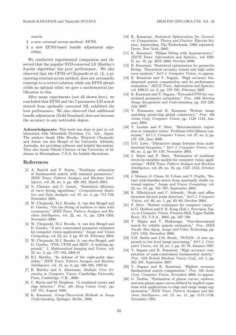
The fundamental matrix is optimally computedwithout considering the rank constraint and ismodified in an optimal manner so that the con-straint is satisfied (Fig. 1(a)).

Internal access

The fundamental matrix is minimally parame-terized so that the rank constraint is identicallysatisfied and is optimized in the reduced (“inter-nal”) parameter space (Fig. 1(b)).

External access

We do iterations in the redundant (“external”)parameter space in such a way that an optimalsolution that satisfies the constraint automati-cally results (Fig. 1(c)).

In this paper, we review existing methods in thisframework and propose new methods. The originalityof this paper is in the following four points:

1. We present a new 7-parameter LM search tech-nique as an internal access method1.

2. We present a new external access method called“EFNS”2.

1A preliminary version was presented in our conference pa-per [24].

2A preliminary version was presented in a more abstractform in our conference paper [14].

18

Kenichi KANATANI and Yasuyuki SUGAYA MEM.FAC.ENG.OKA.UNI. Vol. 42

det F = 0SVD correctionoptimal correction

det F = 0 det F = 0

(a) (b) (c)

Figure 1: (a) A posteriori correction. (b) Internal access. (c) External access.

3. We present a new compact bundle adjustment al-gorithm involving the fundamental matrix aloneusing EFNS3.

4. We experimentally compare the performance ofexisting and proposed methods by doing numer-ical experiments using simulated and real im-ages4.

In Section 2, we summarize the mathematicalbackground. In Section 3, we study the a poste-riori correction approach. We review two correc-tion schemes (SVD correction and optimal correc-tion), three unconstrained optimization techniques(FNS, HEIV, projective Gauss-Newton iterations),and two initialization methods (least squares (LS)and the Taubin method). In Section 4, we focus onthe internal access approach and present a compactscheme for doing 7-parameter Levenberg-Marquardt(LM) search. In Section 5, we investigate the externalaccess approach and point out that the CFNS of Cho-jnacki et al. [4], a pioneering external access method,does not necessarily converge to a correct solution.To complement this, we present a new method calledEFNS and demonstrate that it always converges to anoptimal value; a mathematical justification is givento this. In Section 6, we compare the accuracy of allthe methods and conclude that our EFNS and the7-parameter LM search started from optimally cor-rected ML exhibit the best performance. In Section7, we study the bundle adjustment (Gold Standard)approach and present a new efficient computationalscheme for it. In Section 8, we experimentally test theeffect of this approach and conclude that additionalbundle adjustment does not increase the accuracy toany noticeable degree. Section 9 concludes this paper.

2. Mathematical Fundamentals

Fundamental matrix. We are given two imagesof the same scene. We take the image origin (0, 0)at the frame center. Suppose a point (x, y) in thefirst image corresponds to (x′, y′) in the second. We

3This has not been published anywhere yet.4Part of the numerical results were shown in our conference

paper [25], but the EFNS-based bundle adjustment was notincluded there.

represent them by 3-D vectors

x =

x/f0

y/f0

1

, x′ =

x′/f0

y′/f0

1

, (1)

where f0 is a scaling constant of the order of the imagesize5. As is well known, x and x′ satisfy the epipolarequation [7],

(x, Fx′) = 0, (2)

where and hereafter we denote the inner product ofvectors a and b by (a, b). The matrix F = (Fij) in(2) is of rank 2 and called the fundamental matrix ; itdepends on the relative positions and orientations ofthe two cameras and their intrinsic parameters (e.g.,their focal lengths) but not on the scene or the choiceof the corresponding points. If we define6

u = (F11, F12, F13, F21, F22, F23, F31, F32, F33)>, (3)ξ = (xx′, xy′, xf0, yx′, yy′, yf0, f0x

′, f0y′, f2

0 )>, (4)

we can rewrite (2) as

(u, ξ) = 0. (5)

The magnitude of u is indeterminate, so we normalizeit to ‖u‖ = 1, which is equivalent to scaling F sothat ‖F ‖ = 17. With a slight abuse of symbolism, wehereafter denote by “detu” the determinant of thematrix F defined by u. If we write N observed noisycorrespondence pairs as 9-D vectors {ξα} in the form(4), our task is to estimate from {ξα} a 9-D vector uthat satisfies (5) subject to the constraints ‖u‖ = 1and detu = 0.

Covariance matrices. Let us write ξα = ξα +∆ξα,where ξα is the true value and ∆ξα the noise term.The covariance matrix of ξα is defined by

V [ξα] = E[∆ξα∆ξ>α ], (6)

where E[ · ] denotes expectation over the noise distri-bution. If the noise in the x- and y-coordinates is

5This is for stabilizing numerical computation [6]. In ourexperiments, we set f0 = 600 pixels.

6The vector ξ is known as the “Kronecker product” of thevectors (x, y, f0)> and (x′, y′, f0)>.

7In this paper, we use the Euclidean (or l2) norm for vectorsand the Frobenius norm for matrices.

19

January 2008 Fundamental Matrix Computation: Theory and Practice

O

u

u

P u U

T (U)u

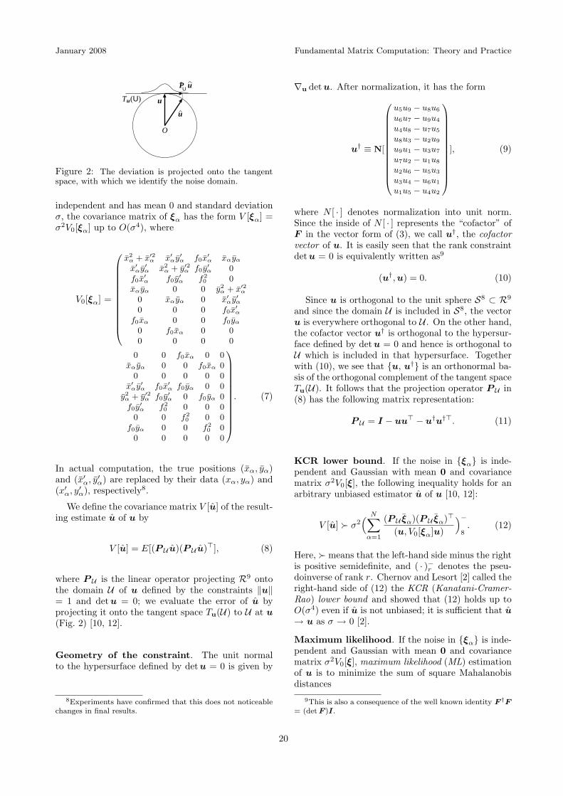
Figure 2: The deviation is projected onto the tangentspace, with which we identify the noise domain.

independent and has mean 0 and standard deviationσ, the covariance matrix of ξα has the form V [ξα] =σ2V0[ξα] up to O(σ4), where

V0[ξα] =

0

B

B

B

B

B

B

B

B

B

B

B

B

@

x2α + x′2

α x′αy′

α f0x′α xαyα

x′αy′

α x2α + y′2

α f0y′α 0

f0x′α f0y

′α f2

0 0xαyα 0 0 y2

α + x′2α

0 xαyα 0 x′αy′

α

0 0 0 f0x′α

f0xα 0 0 f0yα

0 f0xα 0 00 0 0 0

0 0 f0xα 0 0xαyα 0 0 f0xα 0

0 0 0 0 0x′

αy′α f0x

′α f0yα 0 0

y2α + y′2

α f0y′α 0 f0yα 0

f0y′α f2

0 0 0 00 0 f2

0 0 0f0yα 0 0 f2

0 00 0 0 0 0

1

C

C

C

C

C

C

C

C

C

C

C

C

A

. (7)

In actual computation, the true positions (xα, yα)and (x′

α, y′α) are replaced by their data (xα, yα) and

(x′α, y′

α), respectively8.

We define the covariance matrix V [u] of the result-ing estimate u of u by

V [u] = E[(P U u)(P U u)>], (8)

where P U is the linear operator projecting R9 ontothe domain U of u defined by the constraints ‖u‖= 1 and det u = 0; we evaluate the error of u byprojecting it onto the tangent space Tu(U) to U at u(Fig. 2) [10, 12].

Geometry of the constraint. The unit normalto the hypersurface defined by detu = 0 is given by

8Experiments have confirmed that this does not noticeablechanges in final results.

∇u det u. After normalization, it has the form

u† ≡ N[

0

B

B

B

B

B

B

B

B

B

B

B

B

@

u5u9 − u8u6

u6u7 − u9u4

u4u8 − u7u5

u8u3 − u2u9

u9u1 − u3u7

u7u2 − u1u8

u2u6 − u5u3

u3u4 − u6u1

u1u5 − u4u2

1

C

C

C

C

C

C

C

C

C

C

C

C

A

], (9)

where N [ · ] denotes normalization into unit norm.Since the inside of N [ · ] represents the “cofactor” ofF in the vector form of (3), we call u†, the cofactorvector of u. It is easily seen that the rank constraintdetu = 0 is equivalently written as9

(u†, u) = 0. (10)

Since u is orthogonal to the unit sphere S8 ⊂ R9

and since the domain U is included in S8, the vectoru is everywhere orthogonal to U . On the other hand,the cofactor vector u† is orthogonal to the hypersur-face defined by detu = 0 and hence is orthogonal toU which is included in that hypersurface. Togetherwith (10), we see that {u, u†} is an orthonormal ba-sis of the orthogonal complement of the tangent spaceTu(U). It follows that the projection operator P U in(8) has the following matrix representation:

P U = I − uu> − u†u†>. (11)

KCR lower bound. If the noise in {ξα} is inde-pendent and Gaussian with mean 0 and covariancematrix σ2V0[ξ], the following inequality holds for anarbitrary unbiased estimator u of u [10, 12]:

V [u] Â σ2( N∑

α=1

(P U ξα)(P U ξα)>

(u, V0[ξα]u)

)−

8. (12)

Here, Â means that the left-hand side minus the rightis positive semidefinite, and ( · )−r denotes the pseu-doinverse of rank r. Chernov and Lesort [2] called theright-hand side of (12) the KCR (Kanatani-Cramer-Rao) lower bound and showed that (12) holds up toO(σ4) even if u is not unbiased; it is sufficient that u→ u as σ → 0 [2].

Maximum likelihood. If the noise in {ξα} is inde-pendent and Gaussian with mean 0 and covariancematrix σ2V0[ξ], maximum likelihood (ML) estimationof u is to minimize the sum of square Mahalanobisdistances

9This is also a consequence of the well known identity F †F= (det F )I.

20


J =N∑

α=1

(ξα − ξα, V0[ξα]−4 (ξα − ξα)), (13)

subject to (u, ξα) = 0, α = 1, ..., N . Geometri-cally, we are fitting a hyperplane (u, ξ) = 0 in theξ-space to N points {ξα} as closely as possible; thecloseness is measured in the Mahalanobis distance,the distance weighted by the −1/2th power of the co-variance matrix V0[ξα] representing the uncertaintyof each datum.

Eliminating the constraints (u, ξα) = 0 by usingLagrange multipliers, we obtain [10, 12]

J =N∑

α=1

(u, ξα)2

(u, V0[ξα]u). (14)

The ML estimator u minimizes this subject to thenormalization ‖u‖ = 1 and the rank constraint(u†, u) = 0.

3. A Posteriori Correction

3.1 Correction schemes

The a posteriori correction approach first mini-mizes (14) without considering the rank constraintand then modifies the resulting solution u so as tosatisfy it (Fig. 1(a)).

SVD correction. A naive idea is to compute thesingular value decomposition (SVD) of the computedfundamental matrix and replace the smallest singularvalue by 0, resulting in a matrix of rank 2 “closest” inthe Frobenius norm [6]. We call this SVD correction.

Optimal correction. A more sophisticated methodis the optimal correction [10, 18]. According to thestatistical optimization theory [10], the covariancematrix V [u] of the rank unconstrained solution u canbe evaluated, so u is moved in the direction of themostly likely fluctuation implied by V [u] until it sat-isfies the rank constraint (Fig. 1(a)). The proceduregoes as follows [10]:

1. Compute the following 9 × 9 matrix M :

M =N∑

α=1

ξαξ>α

(u, V0[ξα]u). (15)

2. Compute the matrix V0[u] as follows:

V0[u] = M−8 . (16)

3. Update the solution u as follows (u† is the co-factor vector of u):

u ← N [u − 13

(u, u†)V0[u]u†

(u†, V0[u]u†)]. (17)

4. If (u, u†) ≈ 0, return u and stop. Else, updatethe matrix V0[u] in the form

Pu = I − uu>, V0[u] ← PuV0[u]P u, (18)

and go back to Step 3.

Explanation. Since u is a unit vector, its endpointis on the unit sphere S8 in R9. Essentially, (17) isthe Newton iteration formula for displacing u in thedirection in the tangent space Tu(S8) along whichJ is least increased so that (u†, u) = 0 is satisfied.However, u deviates from S8 by a high order smalldistance as it proceeds in Tu(S8), so we “pull” it backonto S8 using the operator N [ · ]. From that point, thesame procedure is repeated until (u†, u) = 0. How-ever, the normalized covariance matrix V0[u] is de-fined in the tangent space Tu(S8), which changes asu moves. So, (18) corrects it so that V0[u] has thedomain Tu(S8) at the displaced point u.

3.2Unconstrained ML

Before imposing the rank constraint, we need to dounconstrained minimization of (14), for which manymethods exist including FNS [3], HEIV [16], and theprojective Gauss-Newton iterations [13]. Their con-vergence properties were studied in [13].

FNS. The FNS (Fundamental Numerical Scheme)of Chojnacki et al. [3] is based on the fact that thederivative of (14) with respect to u has the form

∇uJ = 2Xu, (19)

where X has the following form [3]:

X = M − L, (20)

M =N∑

α=1

ξαξ>α

(u, V0[ξα]u), L =

N∑α=1

(u, ξα)2V0[ξα](u, V0[ξα]u)2

.

(21)The FNS solves

Xu = 0. (22)

by the following iterations [3, 13]:

1. Initialize u.2. Compute the matrix X in (20).3. Solve the eigenvalue problem

Xu′ = λu′, (23)

and compute the unit eigenvector u′ for thesmallest eigenvalue λ.

4. If u′ ≈ u up to sign, return u′ and stop. Else,let u ← u′ and go back to Step 2.

21


Originally, the eigenvalue closest to 0 was chosen [3]in Step 3. Later, Chojnacki, et al. [5] pointed outthat the choice of the smallest eigenvalue improvesthe convergence. This was also confirmed by the ex-periments of Kanatani and Sugaya [13]. Whichevereigenvalue is chosen as λ, we have λ = 0 after conver-gence. In fact, convergence means

Xu = λu (24)

for some u. Computing the inner product with u onboth sides, we have

(u,Xu) = λ, (25)

but from (20) and (21) we have the identity (u,Xu)= 0 in u. Hence, λ = 0, and u is the desired solu-tion10.

HEIV. We can rewrite (22) as

Mu = Lu. (26)

We introduce a new 8-D parameter vector v, 8-D datavectors zα, and their 8×8 normalized covariance ma-trices V0[zα] in the form

ξα =(

zα

f20

), u =

(v

F33

),

V0[ξα] =(

V0[zα] 00> 0

). (27)

We define 8 × 8 matrices

M =N∑

α=1

zαz>α

(v, V0[zα]v), L =

N∑α=1

(v, zα)2V0[zα](v, V0[zα]v)2

,

(28)where we put

zα = zα − z,

z =N∑

α=1

zα

(v, V0[zα]v)

/N∑

β=1

1(v, V0[zβ ]v)

. (29)

Then, (26) splits into the following two equations [5,16]:

Mv = Lv, (v, z) + f20 F33 = 0. (30)

Hence, if an 8-D vector v that satisfies the first equa-tion is computed, the second equation gives F33, andwe obtain

u = N[(

vF33

)]. (31)

The HEIV (Heteroscedastic Errors-in-Variable) ofLeedan and Meer [16] computes the vector v thatsatisfies the first equation in (30) by the followingiterations [5, 16]:

10This crucial fact is inherited to our EFNS to be proposedin Section 5 and plays an essential role for its justification.

1. Initialize v.2. Compute the matrices M and L in (28).3. Solve the generalized eigenvalue problem

Mv′ = λLv′, (32)

and compute the unit generalized eigenvector v′

for the smallest generalized eigenvalue λ.4. If v′ ≈ v except for sign, return v′ and stop.

Else, let v ← v′ and go back to Step 2.

In order to reach the solution of (30), it appears nat-ural to choose as the generalized eigenvalue λ in (32)the one closest to 1. However, Leedan and Meer [16]observed that choosing the smallest one improves theconvergence performance. This was also confirmedby the experiments of Kanatani and Sugaya [13].Whichever generalized eigenvalue is chosen as λ, wehave λ = 1 after convergence. In fact, convergencemeans

Mv = λLv (33)

for some v. Computing the inner product of bothsides with v, we have

(v, Mv) = λ(v, Lv), (34)

but from (28) we have the identity (v, Mv) = (v, Lv)in v. Hence, λ = 1, and u is the desired solution.

Projective Gauss-Newton iterations. Since thegradient ∇uJ is given by (19), we can minimize J byNewton iterations. If we evaluate the Hessian ∇2

uJ ,the increment ∆u in u is determined by solving

(∇2uJ)∆u = −∇uJ. (35)

Since J is constant in the direction of u (see (14)),the Hessian ∇2

uJ is singular, so (35) has infinitelymany solutions. From among them, we choose theone orthogonal to u, using the Moore-Penrose pseu-doinverse and computing

∆u = −(∇2uJ)−8 ∇uJ. (36)

Differentiating (19) and introducing Gauss-Newton approximation (i.e., ignoring terms that con-tain (u, ξα)), we see that the Hessian is nothing butthe matrix 2M in (21). We enforce M to have eigen-value 0 for u, using the projection matrix

P u = I − uu> (37)

onto the direction orthogonal to u. The iteration pro-cedure goes as follows:

1. Initialize u.2. Compute

u′ = N [u − (P uMP u)−8 (M − L)u]. (38)

3. If u′ ≈ u, return u′ and stop. Else, let u ← u′

and go back to Step 2.

22


3.3 Initialization

The FNS, the HEIV, and the projective Gauss-Newton are all iterative method, so they require ini-tial values. The best known non-iterative proceduresare the least squares and the Taubin method.

Least squares (LS). This is the most popularmethod, also known as the algebraic distance mini-mization or the 8-point algorithm [6]. Approximatingthe denominators in (14) by a constant, we minimize

JLS =N∑

α=1

(u, ξα)2 = (u, MLSu), (39)

where we define

MLS =N∑

α=1

ξαξ>α . (40)

The function JLS can be minimized by the unit eigen-vector of MLS for the smallest eigenvalue.

Taubin method. Replacing the denominators in(14) by their average, we minimize the following func-tion11 [26]:

JTB =∑N

α=1(u, ξα)2∑Nα=1(u, V0[ξα]u)

=(u,MLSu)(u, NTBu)

. (41)

The matrix NTB has the form

NTB =N∑

α=1

V0[ξα]. (42)

The function JTB can be minimized by solving thegeneralized eigenvalue problem

MLSu = λNTBu (43)

for the smallest generalized eigenvalue. However, wecannot directly solve this, because NTB is not posi-tive definite. So, we decompose ξα, u, and V0[ξα] inthe form of (27) and define 8 × 8 matrices MLS andNTB by

MLS =N∑

α=1

zαz>α , NLS =

N∑α=1

V0[zα], (44)

where

zα = zα − z, z =1N

N∑α=1

zα. (45)

Then, (43) splits into two equations

MLSv = λNTBv, (v, z) + f20 F33 = 0. (46)

11Taubin [26] did not take the covariance matrix into ac-count. This is a modification of his method.

We compute the unit generalized eigenvector v of thefirst equation for the smallest generalized eigenvalueλ. The second equation gives F33, and u is given inthe form of (31). It has been shown that the Taubinmethod produces a very accurate close to the uncon-strained ML solution [12, 13].

4. Internal Access

The fundamental matrix F has nine elements, onwhich the normalization ‖F ‖ = 1 and the rank con-straint detu = 0 are imposed. Hence, it has seven de-grees of freedom. The internal access approach min-imizes (14) by searching the reduced 7-D parameterspace (Fig. 1(b)).

Many types of 7-degree parameterizations havebeen obtained, e.g., by algebraic elimination of therank constraint or by expressing the fundamental ma-trix in terms of epipoles [22, 28], but the resulting ex-pressions are complicated, and the geometric mean-ing of the individual unknowns are not clear. Thiswas overcome by Bartoli and Sturm [1], who regardedthe SVD of F as its parameterization. Their expres-sion is compact, and each parameter has its geometricmeaning. However, they included, in addition to F ,the tentatively reconstructed 3-D positions of the ob-served feature points, the relative positions of the twocameras, and their intrinsic parameters as unknownsand minimized the reprojection error; such an ap-proach is known as bundle adjustment. Since the ten-tative 3-D reconstruction from two images is indeter-minate, they chose the one for which the first cameramatrix is in a particular form (“canonical form”).

Here, we avoid this complication by directlyminimizing (14) by the Levenberg-Marquardt (LM)method, using the parameterization of Bartoli andSturm [1]

F = Udiag(σ1, σ2, 0)V >, (47)

where U and V are orthogonal matrices, and σ1 andσ2 are the singular values. Since the normalization‖F ‖2 = 1 is equivalent to σ2

1 + σ22 = 1 (see Appendix

A), we adopt the following representation12:

σ1 = cos θ, σ2 = sin θ. (48)

If the principal point is at the origin (0, 0) and if thereare no image distortions, θ takes the value π/4 (i.e.,σ1 = σ2) [7, 10].

The orthogonal matrices U and V have three de-grees of freedom each, so they and θ constitute theseven degrees of freedom. However, the analysis be-comes complicated if U and V are directly expressedin three parameters each (e.g., the Euler angles orthe rotations around each coordinate axis). Follow-ing Bartoli and Sturm [1], we adopt the “Lie algebraic

12Bartoli and Sturm [1] took the ratio γ = σ2/σ1 as a vari-able. Here, we adopt the angle θ for the symmetry.

23


method” [9]: we represent the “increment” in U andV by three parameters each. Let ω1, ω2, and ω3 rep-resent the increment in U , and ω′

1, ω′2, and ω′

3 in V .The derivatives of (14) with respect to them are asfollows (see Appendix A):

∇ωJ = 2F>UXu, ∇ω′J = 2F>

V Xu. (49)

Here, X is the matrix in (20), and F U , and F V aredefined by

F U =

0

B

B

B

B

B

B

B

B

B

B

B

B

@

0 F31 −F21

0 F32 −F22

0 F33 −F23

−F31 0 F11

−F32 0 F12

−F33 0 F13

F21 −F11 0F22 −F12 0F23 −F13 0

1

C

C

C

C

C

C

C

C

C

C

C

C

A

,

F V =

0

B

B

B

B

B

B

B

B

B

B

B

B

@

0 F13 −F12

−F13 0 F11

F12 −F11 00 F23 −F22

−F23 0 F21

F22 −F21 00 F33 −F32

−F33 0 F31

F32 −F31 0

1

C

C

C

C

C

C

C

C

C

C

C

C

A

. (50)

The derivative of (14) with respect to θ has the form(see Appendix A)

∂J

∂θ= (uθ, Xu), (51)

where we define

uθ =

0

B

B

B

B

B

B

B

B

B

B

B

B

@

U12V12 cos θ − U11V11 sin θU12V22 cos θ − U11V21 sin θU12V32 cos θ − U11V31 sin θU22V12 cos θ − U21V11 sin θU22V22 cos θ − U21V21 sin θU22V32 cos θ − U21V31 sin θU32V12 cos θ − U31V11 sin θU32V22 cos θ − U31V21 sin θU32V32 cos θ − U31V31 sin θ

1

C

C

C

C

C

C

C

C

C

C

C

C

A

. (52)

Adopting Gauss-Newton approximation, whichamounts to ignoring terms involving (u, ξα), we ob-tain the second derivatives as follows (see AppendixA):

∇2ωJ = 2F>

UMF U , ∇2ω′J = 2F>

V MF V ,

∇ωω′J = 2F>UMF V ,

∂J2

∂θ2= 2(uθ,Muθ),

∂∇ωJ

∂θ= 2F>

UMuθ,∂∇ω′J

∂θ= 2F>

V Muθ. (53)

The 7-parameter LM search goes as follows:

1. Initialize F = Udiag(cos θ, sin θ, 0)V >.2. Compute J in (14), and let c = 0.0001.3. Compute F U , F V , and uθ in (50) and (52).4. Compute X in (20), the first derivatives in (49)

an (51), and the second derivatives in (53).5. Compute the following matrix H:

H =

∇2ωJ ∇ωω′J ∂∇ωJ/∂θ

(∇ωω′J)> ∇2ω′J ∂∇ω′J/∂θ

(∂∇ωJ/∂θ)> (∂∇ω′J/∂θ)> ∂J2/∂θ2

.

(54)6. Solve the 7-D simultaneous linear equations

(H + cD[H])

ωω′

∆θ

= −

∇ωJ∇ω′J∂J/∂θ

, (55)

for ω, ω′, and ∆θ, where D[ · ] denotes the di-agonal matrix obtained by taking out only thediagonal elements.

7. Update U , V , and θ by

U ′ = R(ω)U , V ′ = R(ω′)V , θ′ = θ + ∆θ,(56)

where R(ω) denotes rotation around N [ω] byangle ‖ω‖.

8. Update F as follows:

F ′ = U ′diag(cos θ′, sin θ′, 0)V ′>. (57)

9. Let J ′ be the value of (14) for F ′.10. Unless J ′ < J or J ′ ≈ J , let c ← 10c, and go

back to Step 6.11. If F ′ ≈ F , return F ′ and stop. Else, let F ←

F ′, U ← U ′, V ← V ′, θ ← θ′, and c ← c/10,and go back to Step 3.

5. External Access

The external access approach does iterations in the9-D u-space in such a way that an optimal solutionsatisfying the rank constraint automatically results(Fig. 1(c)). The concept dates back to such heuristicsas introducing penalties to the violation of the con-straints or projecting the solution onto the surface ofthe constraints in the course of iterations, but it isChojnacki et al. [4] that first presented a systematicscheme called CFNS.

Stationarity Condition. According to the varia-tional principle, the necessary and sufficient condi-tion for the function J to be stationary at a point uin S8 in R9 is that its gradient ∇uJ is orthogonal tothe hypersurface defined by detu = 0 (or equivalentlyby (10)); its surface normal is given by the cofactorvector u†, which is orthogonal to u (see (10)). How-ever, ∇uJ = Xu is always tangent to S8, because ofthe identity (u,∇uJ) = (u, Xu) = 0 in u. So, ∇uJ

24


should be parallel to the cofactor vector u†. Thismeans that if we define the projection matrix

P u† = I − u†u†> (58)

onto the direction orthogonal to the cofactor vectoru†, the stationarity condition is written as

P u†Xu = 0. (59)

The rank constraint of (10) is written as P u†u = u.Combined with (59), the desired solution should besuch that

Y u = 0, P u†u = u, (60)

where we define

Y = P u†XP u† . (61)

CFNS. Chojnacki et al. [4] showed that the station-arity condition of (60) is written as a single equationin the form

Qu = 0, (62)

where Q is a rather complicated symmetric matrix(see Appendix B). They proposed to solve (62) byiterations in the same form as their FNS and calledit CFNS (Constrained FNS ):

1. Initialize u.2. Compute the matrix Q.3. Solve the eigenvalue problem

Qu′ = λu′, (63)

and compute the unit eigenvector u′ for theeigenvalue λ closest to 0.

4. If u′ ≈ u up to sign, return u′ and stop. Else,let u ← u′, and go back to Step 2.

Infinitely many candidates exist for the matrix Qwith which the problem is written as (62), but notall of them allow the above iterations to converge.Chojnacki et al. [4] gave the one shown in AppendixB, but the derivation is not written in their paper. Welater show that CFNS does not necessarily convergeto a correct solution.

EFNS. We now present a new iterative scheme,which we call EFNS (Extended FNS ), for solving(60). The procedure goes as follows:

1. Initialize u.2. Compute the matrix X in (20), the projection

matrix P u† in (58), and the matrix Y in (61).3. Solve the eigenvalue problem

Y v = λv, (64)

and compute the two unit eigenvectors v1 and v2

for the smallest eigenvalues in absolute terms.

4. Compute the following vector u:

u = (u, v1)v1 + (u, v2)v2. (65)

5. Computeu′ = N [P u†u]. (66)

6. If u′ ≈ u, return u′ and stop. Else, let u ←N [u + u′] and go back to Step 2.

Justification. We first show that when the aboveiterations have converged, the eigenvectors v1 and v2

both have eigenvalue 0. From the definition of Y in(61) and P u† in (58), the cofactor vector u† is alwaysan eigenvector of Y with eigenvalue 0. This meansthat either v1 or v2 has eigenvalue 0. Suppose one,say v1, has nonzero eigenvalue λ (6= 0). Then, v2 =±u†.

By construction, the vector u in (65) belongs tothe linear span of v1 and v2 (= ±u†), which are mu-tually orthogonal, and the vector u′ in (66) is a pro-jection of u within that linear span onto the directionorthogonal to the cofactor vector u†. Hence, it coin-cides with ±v1. After the iterations have converged,we have u = u′ (= ±v1), so v1 is an eigenvector of Ywith eigenvalue λ. Hence, u also satisfies (64). Com-puting the inner product with u on both sides, wehave

(u, Y u) = λ. (67)

On the other hand, u (= ±v1) is orthogonal to thecofactor vector u† (= ±v2), so

P u†u = u. (68)

Hence,

(u, Y u) = (u, P u†XP u†u) = (u, Xu) = 0, (69)

since (u,Xu) = 0 is an identity in u (see (20) andalso (21) and footnote 10). However, (67) and (69)contradict our assumption that λ 6= 0. So, v1 is alsoan eigenvector of Y with eigenvalue 0. 2

It follows that the two equations in (60) hold, andhence u is the desired solution. Of course, this conclu-sion relies on the premise that the iterations converge.According to our experience, if we let u ← u′ in Step9, the next value of u′ computed in Step 8 often re-verts to the former value of u, falling in infinite loop-ing. So, we update u to the “midpoint” (u′ + u)/2and normalized it to a unit vector N [u′+u] in Step 9.The convergence performance is greatly improved bythis. In fact, we have observed that this same tech-nique can also improve the convergence performanceof the ordinary FNS, which sometimes oscillates inthe presence of very large noise.

CFNS vs. EFNS. Fig. 3 shows simulated images oftwo planar grid surfaces viewed from different angles.

25


Figure 3: Simulated images of planar grid surfaces.

-0.01

0

0.01

0.03

0.05

0 1 2 3 4 5 6 7 8

det F

0

20

40

60

0 1 2 3 4 5 6 7 8

J

Figure 4: The convergence of det F and the residual Jfor different initializations (σ = 1): LS (solid line), SVD-corrected LS (dashed line), and the true value (chainedline). All solutions are SVD-corrected in the final step.

-0.03

-0.02

-0.01

0

0.01

0 1 2 3 4 5 6 7 8

det F

0

20

40

60

0 1 2 3 4 5 6 7 8

J

Figure 5: The results by EFNS corresponding to Fig. 5.

The image size is 600×600 pixels with 1200 pixel focallength. We added random Gaussian noise of mean 0and standard deviation σ to the x- and y-coordinatesof each grid point independently and from them com-puted the fundamental matrix by CFNS and EFNS.

Fig. 4 shows a typical instance (σ = 1) of the con-vergence of the determinant det F and the residual Jfrom different initial values. In the final step, detFis forced to be 0 by SVD, as prescribed by Chojnackiet al. [4]. The dotted lines show the values to beconverged.

The LS solution has a very low residual J , since therank constraint detF = 0 is ignored. So, J needs tobe increased to achieve det F = 0, but CFNS fails todo so. As a result, det F remains nonzero and dropsto 0 by the final SVD correction, causing a suddenjump in J . If we start from SVD-corrected LS, theresidual J first increases, making det F nonzero, butin the end both J and detF converge in an expectedway. In contrast, the true value has a very large J , soCFNS tries to decrease it sharply at the cost of toomuch increase in detF , which never reverts to 0 untilthe final SVD. Fig. 5 shows corresponding results byEFNS. Both J and detF converge to their correctvalues with stably attenuating oscillations. Figs. 6

-0.04

-0.02

0

0.02

0.04

0 1 2 3 4 5 6 7 8

det F

0

2000

4000

6000

0 1 2 3 4 5 6 7 8

J

Figure 6: The convergence of det F and the residual Jfor different initializations (σ = 3): LS (solid line), SVD-corrected LS (dashed line), and the true value (chainedline). All solutions are SVD-corrected in the final step.

-0.04

0

0.04

0.08

0 1 2 3 4 5 6 7 8

det F

0

1000

2000

3000

0 1 2 3 4 5 6 7 8

J

Figure 7: The results by EFNS corresponding to Fig. 6.

and 7 show the results corresponding to Fig. 4 and 5for another instance (σ = 3). We can observe similarbehavior of CFNS and EFNS.

We mean by “convergence” the state of the samesolution repeating itself in the course of iterations. Inmathematical terms, the resulting solution is a fixedpoint of the iteration operator, i.e., the procedureto update the current solution. In [4], Chojnacki etal. [4] proved that the solution u satisfying (60) is afixed point of their CFNS. Apparently, they expectedto arrive at that solution by their scheme. As demon-strated by Figs. 4, and 6, however, CFNS has manyother fixed points, and which to arrive at depends oninitialization. In contrast, we have proved that anyfixed point of EFNS is necessarily the desired solu-tion.

6. Accuracy Comparison

Using the simulated images in Fig. 3, we comparethe accuracy of the following methods:

1) SVD-corrected LS (Hartley’s 8-point method)2) SVD-corrected ML3) CFNS of Chojnacki et al.4) Optimally corrected ML5) 7-parameter LM6) EFNS

For brevity, we use the shorthand “ML” for uncon-strained minimization of (14), for which we used theFNS of Chojnacki et al. [3] initialized by LS. We con-firmed that FNS, HEIV, and the projective Gauss-Newton iterations all converged to the same solution(up to rounding errors), although the speed of conver-gence varies (see [13] for the convergence comparison).

26


0

0.1

0.2

0 1 2 3 4σ

1

23

4 6

5

Figure 8: The RMS error D vs. noise level σ for Fig. 3.1) SVD-corrected LS. 2) SVD-corrected ML. 3) CFNS. 4)Optimally corrected ML. 5) 7-parameter LM. 6) EFNS.The dotted line indicates the KCR lower bound.

Figure 9: Simulated images of a spherical grid surface.

We initialized the 7-parameter LM, CFNS, and EFNSby LS. All iterations are stopped when the update ofF is less than 10−6 in norm.

Fig. 8 plots for the noise level σ on the horizontalaxis the following root-mean-square (RMS) error Dcorresponding to (8) over 10000 independent trials:

D =

√√√√ 110000

10000∑a=1

‖P U u(a)‖2. (70)

Here, u(a) is the ath value, and P U is the projectionmatrix in (11); since the solution is normalized intoa unit vector, we measure the deviation of u(a) fromu by orthogonally projecting u(a) onto the tangentspace Tu(U) to U at u (see (8) and Fig. 2). Thedotted line is the value implied by the KCR lowerbound (the trace of the right-hand side of (12)).

Note that the RMS error D describes not the sim-ple “average” of the error but its “variation” fromzero; the computed solution is often very close to thetrue value but sometimes very far from it, and Dmeasures the “standard deviation” of the scatter.

Fig. 9 shows simulated images (600×600 pixels) ofa spherical grid surface viewed from different angles.We did similar experiments, and Fig. 10 shows theresults corresponding to Fig. 8.

Preliminary observations. We can see that SVD-corrected LS (Hartley’s 8-point algorithm) performsvery poorly. We can also see that SVD-corrected MLis inferior to optimally corrected ML, whose accuracyis close to the KCR lower bound. The accuracy ofthe 7-parameter LM is nearly the same as optimallycorrected ML when the noise is small but graduallyoutperforms it as the noise increases. Best perform-ing is EFNS, exhibiting nearly the same accuracy as

0

0.1

0.2

0 1 2σ

1

2

3

4

5

6

Figure 10: The RMS error D vs. noise level σ for Fig. 9.1) SVD-corrected LS. 2) SVD-corrected ML. 3) CFNS. 4)Optimally corrected ML. 5) 7-parameter LM. 6) EFNS.The dotted line indicates the KCR lower bound.

the KCR lower bound. The CFNS performs as poorlyas SVD-corrected ML, because, as we observed in thepreceding section, it is likely to stop at the uncon-strained ML solution (we forced the determinant tobe zero by SVD). Doing many experiments (not allshown here), we have observed that:

i) The EFNS stably achieves the highest accuracyover a wide range of the noise level.

ii) Optimally corrected ML is fairly accurate andvery robust to noise but gradually deterioratesas noise grows.

iii) The 7-parameter LM achieves very high accu-racy when started from a good initial value butis likely to fall into local minima if poorly initial-ized.

The robustness of EFNS and optimally correctedML is due to the fact that the computation is donein the redundant (“external”) u-space, where J hasa simple form of (14). In fact, we have never experi-enced local minima in our experiments. The deteri-oration of optimally corrected ML in the presence oflarge noise is because linear approximation is involvedin (17).

The fragility of the 7-parameter LM is attributedto the complexity of the function J when expressed inseven parameters, resulting in many local minima inthe reduced (“internal”) parameter space, as pointedout in [22].

Thus, the optimal correction of ML and the 7-parameter ML have complementary characteristics,which suggests that the 7-parameter ML started fromoptimally corrected ML may exhibit comparable ac-curacy to EFNS. We now confirm this.

Detailed observations. Fig. 11 compares for theimages in Fig. 3:

1) optimally corrected ML.2) 7-parameter LM started from LS.3) 7-parameter LM started from optimally cor-

rected ML.4) EFNS.

27


0.96

0.98

1

1.02

1.04

1.06

1.08

0 1 2 3 4σ

1

23

4

-2

0

2

4

6

8

10

12

0 1 2 3 4σ

2

1 3

4

(a) (b)

Figure 11: (a) The RMS error relative to the KCR lowerbound and (b) the average residual minus minus (N−7)σ2

for Fig. 3. 1) Optimally corrected ML. 2) 7-parameterLM started from LS. 3) 7-parameter LM started from op-timally corrected ML. 4) EFNS.

0.9

1

1.1

1.2

1.3

1.4

1.5

1.6

1.7

1.8

0 1 2

1

2

3 4

σ-5

0

5

10

15

20

0 1 2

12

3 4

σ

(a) (b)

Figure 12: (a) The RMS error relative to the KCR lowerbound and (b) the average residual minus minus (N−7)σ2

for Fig. 9. 1) Optimally corrected ML. 2) 7-parameterLM started from LS. 3) 7-parameter LM started from op-timally corrected ML. 4) EFNS.

For visual ease, we plot in Fig. 11(a) the ratioD/DKCR of D in (70) to the corresponding KCRlower bound. Fig. 11(b) plots the average residualJ (minimum of (14)). Since direct plots of J nearlyoverlap for all the methods, we display here the dif-ference J − (N − 7)σ2, where N is the number ofcorresponding pairs. This is motivated by the factthat to a first approximation J/σ2 is subject to a χ2

distribution with N−7 degrees of freedom [10], so theexpectation of J is approximately (N − 7)σ2. Fig. 12shows the corresponding results for Fig. 9. We ob-serve:

i) The RMS error of optimally corrected ML in-creases as noise increases, yet the correspondingresidual remains low.

ii) The 7-parameter LM started from LS appears tohave small RMS errors for noise levels for whichthe corresponding residual is high, though.

iii) The accuracy of the 7-parameter LM improves ifstarted from optimally corrected ML, resultingin the accuracy comparable to EFNS.

The seeming contradiction that solutions that arecloser to the true value (measured in the RMS error)have higher residuals J implies that the LM searchfailed to reach the true minimum of J , indicatingexistence of local minima located closer to the truevalue than to the true minimum of J . When started

from optimally corrected ML, the LM search success-fully reaches the true minimum of J , resulting in thesmaller J but larger RMS errors.

RMS vs. KCR Lower Bound. One may wonderwhy the computed RMS errors are sometimes belowthe KCR lower bound. There are several reasons forthis.

The KCR lower bound is shown here for a con-venient reference, but it does not mean that errorsof the values computed by any algorithm should beabove it; it is a lower bound on unbiased estimators.By “estimator”, we mean a function of the data, e.g.,the minimizer of a given cost function. An iterativealgorithm such as LM does not qualify as an estima-tor, since the final value depends not only on the databut also on the starting value; the resulting value maynot be the true minimizer of the cost function. Thus,it may happen, as we have observed, that a solutioncloser to the true value has higher residual.

Next, the KCR lower bound is derived, withoutany approximation [10], from the starting identitythat the expectation of the estimator (as a “func-tion” of the data) should coincide with its true value.This is a very strong identity, from which the KCRlower bound is derived using integral transformationsin the same way as the Cramer-Rao lower bound isfrom the unbiasedness constraint in the framework oftraditional statistical estimation. However, the MLestimator or the minimizer of the function J in (14)may not necessarily be unbiased when the noise islarge. In fact, it has been reported that removingbias from the ML solution can result in better accu-racy (“hyperaccuracy”) for ellipse fitting in the pres-ence of large noise [12, 11].

Finally, the RMS error is computed from “finite”samples, while the KCR lower bound is a theoretical“expectation”. We did 10000 independent trials foreach σ, but the result still has fluctuations. Theoret-ically, the plot should be a smooth function of σ, butzigzags remain to some extent how many samples weuse.

Which is better? We have seen the best perfor-mance exhibited by the 7-parameter ML started fromoptimally corrected ML and by EFNS. Now, we testwhich is really better, using a hybrid method: wetry both methods and choose the solution that hasa smaller residual J . Fig. 13 plots the ratio of eachsolution being chosen for the images in Figs. 3 and 9.As we can see, the two methods are completely evenwith no preference of one to the other.

7. Bundle Adjustment

There is a subtle point to be clarified in the discus-sion of Section 2. The transition from (13) to (14) isexact; no approximation is involved. Although termsof O(σ4) are omitted and the true values are replaced

28


0

1

0 1 2 3 4

0.5

σ 0

1

0 0.5 1 1.5 2

0.5

σ

(a) (b)

Figure 13: The ratio of the solution being chosen for(a) Fig. 3 and (b) for Fig. 9. Solid line: 7-parameter LMstarted from optimally corrected ML. Dashed line: EFNS.

by their data in (7), it is numerically confirmed thatthe final results are not affected in any noticeable way.This is also justified by a simple order analysis: be-cause the numerator on the right-hand side of (14)is O(σ2), while the denominator is O(1), any smallperturbation in the denominator causes only a higherorder perturbation of J .

However, although the “analysis” may be correct,the “interpretation” is not strict. Namely, despitethe fact that (14) is the (squared) Mahalanobis dis-tance in the ξ-space, its minimization can be ML onlywhen the noise in the ξ-space is Gaussian, becausethen and only then is the likelihood proportional toe−J/constant. Strictly speaking, if the noise in the im-age plane is Gaussian, the transformed noise in theξ-space is no longer Gaussian, so the proviso that “Ifthe noise in {ξα} is ...” above (13) (and for the KCRlower bound of (12), too) does not necessarily hold,and minimizing (14) is not strictly ML in the imageplane.

In order to test how much difference is incurredby this, we minimize the Mahalanobis distance in the{x,x′}-space, called the reprojection error . This ap-proach was endorsed by Hartley and Zisserman [7],who called it the Gold Standard . So far, however, nosimple procedure existed for minimizing the repro-jection error subject to the epipolar equation with arank-constrained fundamental matrix. So, this prob-lem has usually been done as search in an “aug-mented” parameter space, as done by Bartoli andSturm [1], computing tentative 3-D reconstructionand adjusting the reconstructed shape, the camerapositions, and the intrinsic parameters so that theresulting projection images are as close to the inputimages as possible. Such a strategy is called bundleadjustment .

Here, we present a new numerical scheme for di-rectly minimizing the reprojection error without ref-erence to any tentative 3-D reconstruction; the com-putation is done solely in the domain of the funda-mental matrix F . We compare its accuracy withthose methods we described so far.

Problem. We minimize the reprojection error

E =N∑

α=1

(‖xα − xα‖2 + ‖x′

α − x′α‖2

), (71)

with respect to xα, x′α, α = 1, ..., N , and F (con-

strained to be ‖F ‖ = 1 and det F = 0) subject to theepipolar equation

(xα, F x′α) = 0, α = 1, ..., N. (72)

First approximation. Instead of estimating xα andx′

α directly, we may alternatively express them as

xα = xα − ∆xα, x′α = x′

α − ∆x′α, (73)

and estimate the correction terms ∆xα and ∆x′α.

Substituting (73) into (71), we have

E =N∑

α=1

(‖∆xα‖2 + ‖∆x′

α‖2). (74)

The epipolar equation of (72) becomes

(xα − ∆xα, F (x′α − ∆x′

α)) = 0. (75)

Ignoring the second order terms in the correctionterms, we obtain to a first approximation

(Fx′α, ∆xα) + (F>xα,∆x′

α) = (xα, Fx′α). (76)

Since the correction terms ∆xα and ∆x′α are con-

strained to be in the image plane, we have the con-straints

(k, ∆xα) = 0, (k, ∆x′α) = 0, (77)

where k ≡ (0, 0, 1)>. Introducing Lagrange multipli-ers for (76) and (77), we obtain ∆xα and ∆x′

α thatminimize (74) as follows (see Appendix C):

∆xα =(xα,Fx′

α)P kFx′α

(Fx′α,P kFx′

α) + (F>xα, P kF>xα),

∆x′α =

(xα, Fx′α)P kF>xα

(Fx′α,P kFx′

α) + (F>xα, P kF>xα). (78)

Here, we define

P k ≡ diag(1, 1, 0). (79)

Substituting (78) into (74), we obtain (see AppendixC)

E =N∑

α=1

(xα, Fx′α)2

(Fx′α, P kFx′

α) + (F>xα, P kF>xα),

(80)

29


which is known as the Sampson error [7]. Supposewe have obtained the matrix F that minimizes (80)subject to ‖F ‖ = 1 and det F = 0. Writing it as Fand substituting it into (78), we obtain

xα = xα − (xα, F x′α)P kF x′

α

(F x′α, P kF x′

α) + (F>

xα, P kF>

xα),

x′α = x′

α − (xα, F x′α)P kF

>xα


α) + (F>

xα, P kF>

xα).

(81)

Second approximation. The solution (81) is only afirst approximation. So, we estimate the true solutionxα and x′

α by writing, instead of (73),

xα = xα − ∆xα, x′α = x′

α − ∆x′α, (82)

and estimating the correction terms ∆xα and ∆x′α,

which are small quantities of higher order than ∆xα

and ∆x′α. Substitution of (82) into (71) yields

E =N∑

α=1

(‖xα + ∆xα‖2 + ‖x′

α + ∆x′α‖2

), (83)

where we define

xα = xα − xα, x′α = x′

α − x′α. (84)

The epipolar equation of (72) now becomes

(xα − ∆xα,F (x′α − ∆x′

α)) = 0. (85)

Ignoring second order terms in ∆xα and ∆x′α, which

are already of high order, we have

(F x′α, ∆xα) + (F>xα, ∆x′

α) = (xα, F x′α). (86)

This is a higher order approximation of (72) than(76). Introducing Lagrange multipliers to (86) andthe constraints

(k, ∆xα) = 0, (k, ∆x′α) = 0, (87)

we obtain ∆xα and ∆x′α that minimize (80) as follows

(see Appendix C):

∆xα =

((xα,F x′

α)+(F x′α,xα)+(F>xα,x′

α))P kF x′

α


α)+(F>xα, P kF>xα)−xα,

∆x′α =

((xα,F x′

α)+(F x′α,xα)+(F>xα,x′

α))P kF>xα


α)+(F>xα, P kF>xα)−x′

α. (88)

On substation of (88), the reprojection error E nowhas the following form (see Appendix C):

E =N∑

α=1

((xα, F x′

α)+(F x′α, xα)+(F>xα, x′

α))2


α) + (F>xα, P kF>xα).

(89)Suppose we have obtained the matrix F that mini-mizes this subject to ‖F ‖ = 1 and det F = 0. Writing

it as ˆF and substituting it into (88), we obtain the

solution

ˆxα = xα

−

((xα,

ˆF x′

α)+( ˆF x′

α,xα)+( ˆF>xα,x′

α))P k

ˆF x′

α

( ˆF x′

α,P kˆF x′

α) + ( ˆF>xα, P k

ˆF>xα)

,

ˆx′α = x′

α

−

((xα,

ˆF x′

α)+( ˆF x′

α,xα)+( ˆF>xα,x′

α))P k

ˆF>xα

( ˆF x′

α, P kˆF x′

α) + ( ˆF>xα, P k

ˆF>xα)

.

(90)

The resulting { ˆxα, ˆx′α} are a better approximation

than {xα, x′α}. Rewriting { ˆxα, ˆx

′α} as {xα, x′

α}, wecan estimate a yet better solution in the form of (82).We repeat this until the iterations converge.

Fundamental matrix computation. The remain-ing problem is to compute the matrix F that mini-mizes (80) and (89) subject to ‖F ‖ = 1 and det F =0. If we use the representation in (3) and (4), we canconfirm the identities

(xα, Fx′α) =

(u, ξα)f20

, (91)

(Fx′α,P kFx′

α)+(F>xα,P kF>xα)=(u,V0[ξα]u)

f20

,

(92)where V0[ξα] is the matrix in (7). Using (91) and(92), the reprojection error E in (80) can be writtenas

E =1f20

N∑α=1

(u, ξα)2

(u, V0[ξα]u), (93)

which is identical to (14) except the scale. The matrixF that minimizes (93) subject to ‖F ‖ = 1 and det F= 0 can be determined by the methods described inSections 3–5.

30


Now, if we define

ξα =

xαx′α + x′

αxα + xαx′α

xαy′α + y′

αxα + xαy′α

f0(xα + xα)yαx′

α + x′αyα + yαx′

α

yαy′α + y′

αyα + yαy′α

f0(yα + yα)f0(x′

α + x′α)

f0(y′α + y′

α)f20

, (94)

we can confirm the identities

(xα,ˆF x′

α)+( ˆF x′

α, xα)+( ˆF>xα, x′

α) =(u, ξα)

f20

, (95)

( ˆFx′

α,P kˆFx′

α)+( ˆF>xα,P k

ˆF>xα)=

(u,V0[ξα]u)f20

,

(96)where V0[ξα] is the matrix obtained by replacing xα,yα, x′

α, and y′α in (7) by xα, y′

α, x′α, and y′

α, respec-tively. Hence, (89) is rewritten as

E =1f20

N∑α=1

(u, ξα)2

(u, V0[ξα]u), (97)

which is again identical to (14) in form except thescale; if xα = xα, the vector ξα in (94) reduces to ξα,and (97) reduces to (93). Thus, the matrix F thatminimizes (97) subject to ‖F ‖ = 1 and detF = 0 canbe determined by the methods in Sections 3–5. Thisis the core discovery of this paper , unnoticed in thepast.

Procedure. Our bundle adjustment computation issummarized as follows.

1. Let u0 = 0.2. Let xα = xα, yα = yα, x′

α = x′α, y′

α = y′α, and

xα = yα = x′α = y′

α = 0.3. Compute the vectors ξα and the matrices V0[ξα].4. Compute the vector u that minimizes

E =1f20

N∑α=1

(u, ξα)2

(u, V0[ξα]u), (98)

subject to ‖u‖ = 1 and (u†, u) = 0.5. If u ≈ u0 up to sign, return u and stop. Else,

update xα, yα, x′α, and y′

α as follows:

xα←(u, ξα)P kF x′

α

(u, V0[ξα]u), x′

α←(u, ξα)P kF>xα

(u, V0[ξα]u).

(99)6. Go back to Step 3 after the following update:

u0 ← u, xα ← xα − xα, yα ← yα − yα,

x′α ← x′

α − x′α, y′

α ← y′α − y′

α. (100)

0

0.1

0.2

0.3

0.4

0 2 4 6 8 10σ 0

0.001

0.002

0.003

0.004

0.005

0 2 4 6 8 10σ

(a) (b)

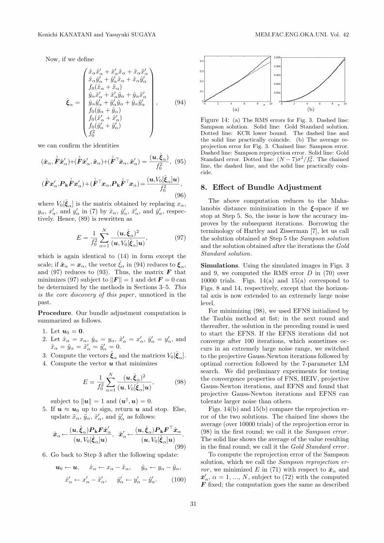
Figure 14: (a) The RMS errors for Fig. 3. Dashed line:Sampson solution. Solid line: Gold Standard solution.Dotted line: KCR lower bound. The dashed line andthe solid line practically coincide. (b) The average re-projection error for Fig. 3. Chained line: Sampson error.Dashed line: Sampson reprojection error. Solid line: GoldStandard error. Dotted line: (N − 7)σ2/f2

0 . The chainedline, the dashed line, and the solid line practically coin-cide.

8. Effect of Bundle Adjustment

The above computation reduces to the Maha-lanobis distance minimization in the ξ-space if westop at Step 5. So, the issue is how the accuracy im-proves by the subsequent iterations. Borrowing theterminology of Hartley and Zisserman [7], let us callthe solution obtained at Step 5 the Sampson solutionand the solution obtained after the iterations the GoldStandard solution.

Simulations. Using the simulated images in Figs. 3and 9, we computed the RMS error D in (70) over10000 trials. Figs. 14(a) and 15(a) correspond toFigs. 8 and 14, respectively, except that the horizon-tal axis is now extended to an extremely large noiselevel.

For minimizing (98), we used EFNS initialized bythe Taubin method at fist; in the next round andthereafter, the solution in the preceding round is usedto start the EFNS. If the EFNS iterations did notconverge after 100 iterations, which sometimes oc-curs in an extremely large noise range, we switchedto the projective Gauss-Newton iterations followed byoptimal correction followed by the 7-parameter LMsearch. We did preliminary experiments for testingthe convergence properties of FNS, HEIV, projectiveGauss-Newton iterations, and EFNS and found thatprojective Gauss-Newton iterations and EFNS cantolerate larger noise than others.

Figs. 14(b) and 15(b) compare the reprojection er-ror of the two solutions. The chained line shows theaverage (over 10000 trials) of the reprojection error in(98) in the first round; we call it the Sampson error .The solid line shows the average of the value resultingin the final round; we call it the Gold Standard error .

To compute the reprojection error of the Sampsonsolution, which we call the Sampson reprojection er-ror , we minimized E in (71) with respect to xα andx′

α, α = 1, ..., N , subject to (72) with the computedF fixed; the computation goes the same as described

31


0

0.1

0.2

0.3

0.4

0 1 2 3 4 5 6 7σ 0

0.01

0.02

0.03

0 1 2 3 4 5 6 7σ

(a) (b)

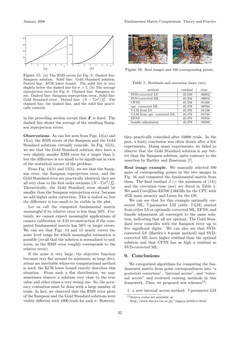
Figure 15: (a) The RMS errors for Fig. 9. Dashed line:Sampson solution. Solid line: Gold Standard solution.Dotted line: KCR lower bound. The solid line is veryslightly below the dashed line for σ > 5. (b) The averagereprojection error for Fig. 9. Chained line: Sampson er-ror. Dashed line: Sampson reprojection error. Solid line:Gold Standard error. Dotted line: (N − 7)σ2/f2

0 . Thechained line, the dashed line, and the solid line practi-cally coincide.

in the preceding section except that F is fixed. Thedashed line shows the average of the resulting Samp-son reprojection errors.

Observations. As can bee seen from Figs. 14(a) and15(a), the RMS errors of the Sampson and the GoldStandard solutions virtually coincide. In Fig. 15(b),we see that the Gold Standard solution does have avery slightly smaller RMS error for σ larger than 5,but the difference is too small to be significant in viewof the statistical nature of the problem.

From Fig. 14(b) and 15(b), we see that the Samp-son error, the Sampson reprojection error, and theGold Standard error are practically identical; they areall very close to the first order estimate (N−7)σ2/f2

0 .Theoretically, the Gold Standard error should besmaller than the Sampson reprojection error, becausewe add higher order correction. This is indeed so, butthe difference is too small to be visible in the plot.

Let us call the computed fundamental matrixmeaningful if its relative error is less than 50%. Cer-tainly, we cannot expect meaningful applications ofcamera calibration or 3-D reconstruction if the com-puted fundamental matrix has 50% or larger errors.We can see that Figs. 14 and 15 nearly covers thenoise level range for which meaningful estimation ispossible (recall that the solution is normalized to unitnorm, so the RMS error roughly corresponds to therelative error).

If the noise is very large, the objective functionbecomes very flat around its minimum, so large devi-ations are inevitable whatever computational methodis used; the KCR lower bound exactly describes thissituation. From such a flat distribution, we maysometimes observe a solution very close to the truevalue and other times a very wrong one. So, the accu-racy evaluation must be done with a large number oftrials. In fact, we observed that the RMS error plotsof the Sampson and the Gold Standard solutions werevisibly different with 1000 trials for each σ. However,

Figure 16: Real images and 100 corresponding points.

Table 1: Residuals and execution times (sec).

method residual time

SVD-corrected LS 45.550 . 00052SVD-corrected ML 45.556 . 00652CFNS 45.556 . 01300opt. corrected ML 45.378 . 007647-LM from LS 45.378 . 011367-LM from opt. corrected ML 45.378 . 01748EFNS 45.379 . 01916bundle adjustment 45.379 . 02580

they practically coincided after 10000 trials. In thepast, a hasty conclusion was often drawn after a fewexperiments. Doing many experiments, we failed toobserve that the Gold Standard solution is any bet-ter than the Sampson solution, quite contrary to theassertion by Hartley and Zisserman [7].

Real image example. We manually selected 100pairs of corresponding points in the two images inFig. 16 and computed the fundamental matrix fromthem. The final residual J (= the minimum of (14))and the execution time (sec) are listed in Table 1.We used Core2Duo E6700 2.66GHz for the CPU with4GB main memory and Linux for the OS.

We can see that for this example optimally cor-rected ML, 7-parameter LM (abbr. 7-LM) startedfrom either LS or optimally corrected ML, EFNS, andbundle adjustment all converged to the same solu-tion, indicating that all are optimal. The Gold Stan-dard error coincides with the Sampson error up tofive significant digits. We can also see that SVD-corrected LS (Hartley’s 8-point method) and SVD-corrected ML have higher residual than the optimalsolution and that CFNS has as high a residual asSVD-corrected ML.

9. Conclusions

We categorized algorithms for computing the fun-damental matrix from point correspondences into “aposteriori correction”, “internal access”, and “exter-nal access” and reviewed existing methods in thisframework. Then, we proposed new schemes13:

1. a new internal access method: 7-parameter LM13Source codes are available at

http://www.iim.ics.tut.ac.jp/˜sugaya/public-e.html

32


search.2. a new external access method: EFNS.3. a new EFNS-based bundle adjustment algo-

rithm.

We conducted experimental comparison and ob-served that the popular SVD-corrected LS (Hartley’s8-point algorithm) has poor performance. We alsoobserved that the CFNS of Chojnacki et al. [4], a pi-oneering external access method, does not necessarilyconverge to a correct solution, while our EFNS alwaysyields an optimal value; we gave a mathematical jus-tification to this.

After many experiments (not all shown here), weconcluded that EFNS and the 7-parameter LM searchstarted from optimally corrected ML exhibited thebest performance. We also observed that additionalbundle adjustment (Gold Standard) does not increasethe accuracy to any noticeable degree.

Acknowledgments: This work was done in part in col-laboration with Mitsubishi Precision, Co. Ldt., Japan.The authors thank Mike Brooks, Wojciech Chojnacki,and Anton van den Hengel of the University Adelaide,Australia, for providing software and helpful discussions.They also thank Nikolai Chernov of the University of Al-abama at Birmingham, U.S.A. for helpful discussions.

References

[1] A. Bartoli and P. Sturm, “Nonlinear estimationof fundamental matrix with minimal parameters,”IEEE Trans. Pattern Analysis and Machine Intel-ligence, vol. 26, no. 3, pp. 426–432, March 2004.

[2] N. Chernov and C. Lesort, “Statistical efficiencyof curve fitting algorithms,” Computational Statis-tics and Data Analysis, vol. 47, no. 4, pp. 713–728,November 2004.

[3] W. Chojnacki, M.J. Brooks, A. van den Hengel andD. Gawley, “On the fitting of surfaces to data withcovariances,” IEEE Trans. Pattern Analysis and Ma-chine Intelligence, vol. 22, no. 11, pp. 1294–1303,November 2000.

[4] W. Chojnacki, M.J. Brooks, A. van den Hengel andD. Gawley, “A new constrained parameter estimatorfor computer vision applications,” Image and VisionComputing , vol. 22, no. 2, pp. 85–91, February 2004.

[5] W. Chojnacki, M.J. Brooks, A. van den Hengel, andD. Gawley, “FNS, CFNS and HEIV: A unifying ap-proach,” J. Mathematical Imaging and Vision, vol.23, no. 2, pp. 175–183, 2005-9)

[6] R.I. Hartley, “In defense of the eight-point algo-rithm,” IEEE Trans. Pattern Analysis and MachineIntelligence, vol. 19, no. 6, pp. 580–593, 1997-6)

[7] R. Hartley and A. Zisserman, Multiple View Ge-ometry in Computer Vision. Cambridge UniversityPress, Cambridge, U.K., 2000.

[8] C. Harris and M. Stephens, “A combined corner andedge detector,” Proc. 4th Alvey Vision Conf., pp.147–151, August 1988.

[9] K. Kanatani, Group-Theoretical Methods in ImageUnderstanding . Springer, Berlin, 1990.

[10] K. Kanatani, Statistical Optimization for Geomet-ric Computation: Theory and Practice. Elsevier Sci-ence, Amsterdam, The Netherlands, 1996; reprinted,Dover, New York, 2005.

[11] K. Kanatani, “Ellipse fitting with hyperaccuracy,”IEICE Trans. Information and Systems,, vol. E89-D, no. 10, pp. 2653–2660, October 2006.

[12] K. Kanatani, “Statistical optimization for geometricfitting: Theoretical accuracy bound and high ordererror analysis,” Int’l J. Computer Vision, to appear.

[13] K. Kanatani and Y. Sugaya, “High accuracy fun-damental matrix computation and its performanceevaluation,” IEICE Trans. Information and Systems,vol. E90-D, no. 2, pp. 579–585, February 2007.

[14] K. Kanatani and Y. Sugaya, “Extended FNS for con-strained parameter estimation,” Proc. 10th MeetingImage Recognition and Understanding , pp. 219–226,July 2007.

[15] Y. Kanazawa and K. Kanatani “Robust imagematching preserving global consistency,” Proc. 6thAsian Conf. Computer Vision, pp. 1128–1133, Jan-uary 2004.

[16] Y. Leedan and P. Meer, “Heteroscedastic regres-sion in computer vision: Problems with bilinear con-straint,” Int’l J. Computer Vision, vol. 37, no. 2, pp.127–150, June 2000.

[17] D.G. Lowe, “Distinctive image features from scale-invariant keypoints, ” Int’l J. Computer Vision, vol.60, no. 2, pp. 91–110, November 2004.

[18] J. Matei and P. Meer, “Estimation of nonlinearerrors-in-variables models for computer vision appli-cations,” IEEE Trans. Pattern Analysis and MachineIntelligence, vol. 28, no. 10, pp. 1537–1552, October2006.

[19] J. Matasu, O. Chum, M. Urban, and T. Pajdla, “Ro-bust wide-baseline stereo from maximally stable ex-tremal regions,” Image and Vision Computing , vol.22, no. 10, pp. 761–767, September 2004.

[20] K. Mikolajczyk and C. Schmidt, “Scale and affineinvariant interest point detectors,” Int’l J. ComputerVision, vol. 60, no. 1, pp. 63–86, October 2004.

[21] P. Meer, “Robust techniques for computer vision,”in G. Medioni and S. B. Kang (Eds.), Emerging Top-ics in Computer Vision. Prentice Hall, Upper SaddleRiver, NJ, U.S.A., 2004, pp. 107–190.

[22] T. Migita and T. Shakunaga, “One-dimensionalsearch for reliable epipole estimation,” Proc. IEEEPacific Rim Symp. Image and Video Technology , pp.1215–1224, December 2006.

[23] S.M. Smith and J.M. Brady, “SUSAN—A new ap-proach to low level image processing,” Int’l J. Com-puter Vision, vol. 23, no. 1, pp. 45–78, January 1997.

[24] Y. Sugaya and K. Kanatani, “High accuracy com-putation of rank-constrained fundamental matrix,”Proc. 18th British Machine Vision Conf., vol. 1, pp.282–291, September 2007.

[25] Y. Sugaya and K. Kanatani, “Highest accuracyfundamental matrix computation,” Proc. 8th AsianConf. Computer Vision, November 2008, to appear.

[26] G. Taubin, “Estimation of planar curves, surfaces,and non-planar space curves defined by implicit equa-tions with applications to edge and range image seg-mentation,” IEEE Trans. Pattern Analysis and Ma-chine Intelligence, vol. 13, no. 11, pp. 1115–1138,November 1991.

33


[27] Z. Zhang, R. Deriche, O. Faugeras and Q.-T. Luong,“A robust technique for matching two uncalibratedimages through the recovery of the unknown epipo-lar geometry,” Artificial Intelligence, vol. 78, pp. 87–119, 1995.

[28] Z. Zhang and C. Loop, “Estimating the fundamentalmatrix by transforming image points in projectivespace,” Computer Vision and Image Understanding ,vol. 82, no. 2, pp. 174–180, May 2001.

Appendix

A. Derivation of the 6-parameter LM

First, note that if F has the form of (47), we seethat

‖F ‖2 =3∑

i,j=1

F 2ij = tr[FF>]

= tr[Udiag(σ1, σ2, 0)V >V diag(σ1, σ2, 0)U>]

= tr[U>Udiag(σ21 , σ2

2 , 0)] = σ21 + σ2

2 , (101)

where we have used the matrix identity tr[AB] =tr[BA] together with the orthogonality V >V = I

and U>U = I. Thus, the parameterization of (48)ensures the normalization ‖F ‖ = 1.

Suppose the orthogonal matrices U and V undergoa small change into U + ∆U and V + ∆V , respec-tively. According to the Lie group theory [9], thereexist small vectors ω and ω′ such that the increments∆U and ∆V are written as

∆U = ω × U , ∆V = ω′ × V (102)

to a first approximation, where the operator × meanscolumn-wise vector product. It follows that the incre-ment ∆F in F is written to a first approximation as

∆F = ω × Udiag(cos θ, sin θ, 0)V >

+Udiag(− sin θ∆θ, cos θ∆θ, 0)V >

+Udiag(cos θ, sin θ, 0)(ω′ × V )>. (103)

Taking out the elements, we can rearrange this in thevector form

∆u = F Uω + uθ∆θ + F V ω′, (104)

where F U and F V are the matrices in (50) and uθ isdefined by (52). The resulting increment ∆J in J iswritten to a first approximation as

∆J = (∇uJ,∆u) = (2Xu, F Uω + uθ∆θ + F V ω′)

= 2(F>UXu, ω) + 2(uθ, Xu)∆θ

+2(F V XuJ,ω′), (105)

which shows that the first derivatives of J are givenby (49) and (51). The second order increment is

∆2J = (∆u,∇2uJ∆u)

= (F Uω+uθ∆θ+F V ω′, 2M(F Uω+uθ∆θ

+F V ω′))

= 2(ω, F>UMF Uω) + 2(ω′, F>

V MF V ω′)

+2(uθ, Muθ)∆θ2 + 4(ω,F>UMω′)

+4(ω, F>UMuθ)∆θ + 4(ω′, F>

V Muθ)∆θ,

(106)

where we have used the Gauss-Newton approxima-tion ∇2

uJ ≈ 2M . From this, we obtain the secondderivatives in (53).

B. Details of CFNS

According to Chojnacki et al. [4], the matrix Q in(62) is given without any reasoning as follows (theiroriginal symbols are altered to conform to the use inthis paper). The gradient ∇uJ = (∂J/∂ui) and theHessian ∇2

uJ = (∂2J/∂ui∂uj) of (14) are

∇uJ = 2(M − L)u, ∇2uJ = 2(M − L) − 8(S − T ),

(107)where M and L are the matrices in (21), and wedefine

S =N∑

α=1

(u, ξα)S[ξα(V0[ξα]u)>](u, V0[ξα]u)2

,

T =N∑

α=1

(u, ξα)2(V0[ξα]u)(V0[ξα]u>)>

(u, V0[ξα]u)3. (108)

Here, S[ · ] is the symmetrization operator (S[A] =(A + A>)/2). Let

A = P u†(∇2uJ)(2uu> − I),

B =2

‖det u‖

( 9∑i=1

S[((∇2u det u)ei)u†>](∇uJ)e>

i

−(u†,∇uJ)u†u†>∇2u detu

),

C = 3( det u

‖∇u det u‖2∇2

u det u

+u†u†>(I − 2 det u

‖∇u det u‖2∇2

u det u))

, (109)

where u† is the cofactor vector of u, P u† is the pro-jection matrix in (58), and ei is the ith coordinatebasis vector (with 0 components except 1 in the ithposition). The matrix Q is given by

Q = (A + B + C)(A + B + C)>. (110)

C. Details of bundle adjustment

Introducing Lagrange multipliers λα, µα, and µ′α

for the constraints of (76), and (77) to (74), we let

L =N∑

α=1

(‖∆xα‖2 + ‖∆x′

α‖2)

34


−N∑

α=1

λα

((Fx′

α, ∆xα) + (F>xα, ∆x′α)

)−

N∑α=1

µα(k, ∆xα) −N∑

α=1

µ′α(k,∆x′

α). (111)

Letting the derivatives of L with respect to ∆xα and∆x′

α be 0, we have

2∆xα − λαFx′α − µαk = 0,

2∆x′α − λαF>xα − µ′

αk = 0. (112)

Multiplying the projection matrix P k in (79) onboth sides from left and noting that P k∆xα = ∆xα,P k∆x′

α = ∆x′α, and P kk = 0, we have

2∆xα − λαP kFx′α = 0, 2∆x′

α − λαP kF>xα = 0.(113)

Hence, we obtain

∆xα =λα

2P kFx′

α, ∆x′α =

λα

2P kF>xα. (114)

Substituting these into (76), we have

(Fx′α,

λα

2P kFx′

α) + (F>xα,λα

2P kF>xα)

= (xα, Fx′α), (115)

and hence

λα

2=

(xα, Fx′α)

(Fx′α, P kFx′

α) + (F>xα, P kF>xα). (116)

Substituting this into (114), we obtain (78). If wesubstitute (78) into (74), we have

E =N∑

α=1

(∥∥∥ (xα, Fx′α)P kFx′

α

(x′α, F>P kFx′

α) + (xα,FP kF>xα)

∥∥∥2

+∥∥∥ (xα, Fx′

α)P kF>xα

(x′α, F>P kFx′

α) + (xα, FP kF>xα)

∥∥∥2)=

N∑α=1

(xα,Fx′α)2(‖P kFx′

α‖2 + ‖P kF>xα‖2)((Fx′

α, P kFx′α) + (F>xα,P kF>xα)

)2

=N∑

α=1

(xα, Fx′α)2

(Fx′α,P kFx′

α)+(F>xα,P kF>xα), (117)

where we have noted due to the identity P 2k

= P k that ‖P kFx′α‖2 = (P kFx′

α, P kFx′α) =

(Fx′α, P 2

kFx′α) = (Fx′

α, P kFx′α). Similarly, we

have ‖P kF>xα‖2 = (F>xα,P kF>xα).Introducing Lagrange multipliers λα, µα, and µ′

α

for the constraints of (85), and (87) to (74), we let

L =N∑

α=1

(‖xα + ∆xα‖2 + ‖x′

α + ∆x′α‖2

)

−N∑

α=1

λα

((F x′

α, ∆xα) + (F>xα, ∆x′α)

)−

N∑α=1

µα(k,∆xα) −N∑

α=1

µ′α(k, ∆x′

α). (118)

Letting the derivatives of L with respect to ∆xα and∆x′

α be 0, we have

2(xα + ∆xα) − λαF x′α − µαk = 0,

2(x′α + ∆x′

α) − λαF>xα − µ′αk = 0. (119)

Multiplying P k on both sides from left, we have

2xα + 2∆xα − λαP kF x′α = 0,

2xα + 2∆x′α − λαP kF>xα = 0. (120)

Substituting these into (86), we have

∆xα =λα

2P kF x′

α− xα, ∆x′α =

λα

2P kF>xα− x′

α.

(121)

Substituting these into (86), we obtain

(F x′α,

λα

2P kF x′

α − xα)

+(F>xα,λα

2P kF>xα − x′

α) = (xα, F x′α), (122)

and hence

λα

2=

(xα,F x′α)+(F x′

α,xα)+(F>xα,x′α)

(F x′α,P kF x′

α)+(F>xα,P kF>xα). (123)

Substituting this into (121), we obtain (89). If wesubstitute (89) into (83), we have

E =N

X

α=1

„

‚

‚

‚

‚

„

(xα, F x′α)+(F x′

α, xα)+(F >xα, x′α)

«

P kF x′α


α) + (F >xα, P kF >xα)

‚

‚

‚

‚

2

+

‚

‚

‚

‚

„

(xα, F x′α)+(F x′

α, xα)+(F >xα, x′α)

«

P kF >xα


α) + (F >xα, P kF >xα)

‚

‚

‚

‚

2«

=N∑

α=1

((xα, F x′


α))2

((F x′

α, P kF x′α) + (F>xα,P kF>xα)

)2

(‖P kF x′

α‖2 + ‖P kF>xα‖2)

=N∑

α=1

((xα, F x′


α))2

(F x′α,P kF x′

α) + (F>xα, P kF>xα).

(124)

35

fundamental matrix computation: theory and …kanatani/papers/okafund.pdfsolution that satisﬁes...

Documents