fundamental fluid mechanics - units.it · 2016-09-14 · 4 1 fundamental fluid mechanics as an...

1A. Kheradvar, G. Pedrizzetti, Vortex Formation in the Cardiovascular System, DOI 10.1007/978-1-4471-2288-3_1, © Springer-Verlag London Limited 2012

Abstract This chapter of the book introduces the basic elements of fl uid mechanics constituting the essential background for understanding the blood fl ow phenomena in the cardiovascular system. It discusses the physics of fl ow and its implications. This chapter is aimed to provide an intuitive understanding, accompanied by an essential mathematical formulation that ensures a rigorous reference ground.

1.1 Fluids and Solids, Blood and Tissues

The most defi nitive property of fl uids, which include liquids and gases, is that a fl uid does not have preferred shape. A fl uid takes the shape of its container regardless of any geometry it had previously. In contrast, a solid consists of constituting elements with a predefi ned shape. When the relative position of these constituent elements is infi nitesimally changed, internal stresses develop to restore the elements to their original, stress-free state. This distinctive property of solids is called elasticity. An elastic deformation typically is completely reversible as the energy stored in the deformed elements is totally released when the deformation ceases.

Fluids, on the other hand, do not share this feature of the solid materials. They have no preferred geometry; thus they possess infi nitely independent, stress-free states. Nevertheless, fl uids exhibit an internal resistance during their relative motion. This resistance is due to the development of internal stresses in response to a “rate of deformation”. This behavior is due to viscosity . Therefore, a fl uid experiences a viscous resistance during the motion, which is caused due to sliding fl uid elements on each other. Given that the viscous stresses represent a frictional phenomenon that appears during motion, when the motion is ceased, no internal stress returns the fl uid to its original state, as in the solids. The mechanical energy that deforms the fl uid elements is not being stored anywhere; it dissipates due to internal viscous friction, which is transformed into heat and

Chapter 1 Fundamental Fluid Mechanics

2 1 Fundamental Fluid Mechanics

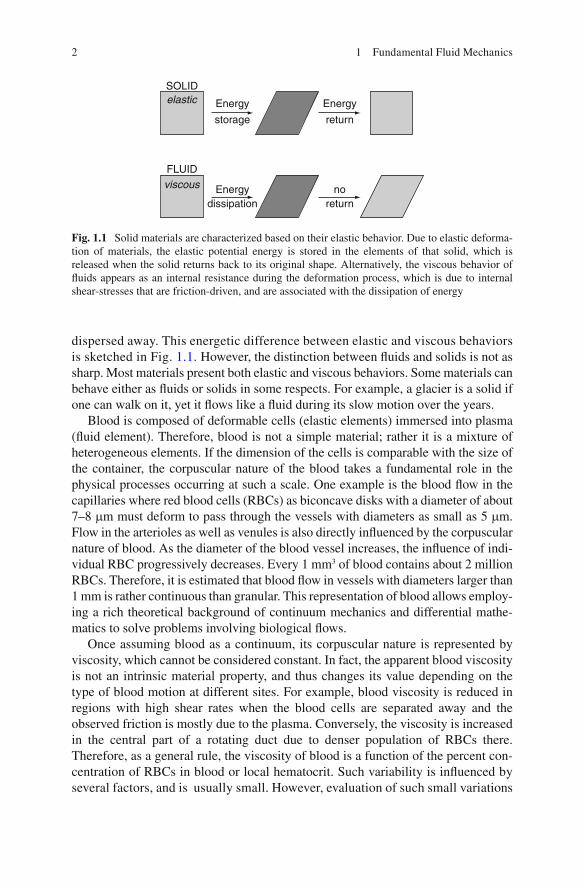
dispersed away. This energetic difference between elastic and viscous behaviors is sketched in Fig. 1.1 . However, the distinction between fl uids and solids is not as sharp. Most materials present both elastic and viscous behaviors. Some materials can behave either as fl uids or solids in some respects. For example, a glacier is a solid if one can walk on it, yet it fl ows like a fl uid during its slow motion over the years.

Blood is composed of deformable cells (elastic elements) immersed into plasma (fl uid element). Therefore, blood is not a simple material; rather it is a mixture of heterogeneous elements. If the dimension of the cells is comparable with the size of the container, the corpuscular nature of the blood takes a fundamental role in the physical processes occurring at such a scale. One example is the blood fl ow in the capillaries where red blood cells (RBCs) as biconcave disks with a diameter of about 7–8 m m must deform to pass through the vessels with diameters as small as 5 m m. Flow in the arterioles as well as venules is also directly infl uenced by the corpuscular nature of blood. As the diameter of the blood vessel increases, the infl uence of indi-vidual RBC progressively decreases. Every 1 mm 3 of blood contains about 2 million RBCs. Therefore, it is estimated that blood fl ow in vessels with diameters larger than 1 mm is rather continuous than granular. This representation of blood allows employ-ing a rich theoretical background of continuum mechanics and differential mathe-matics to solve problems involving biological fl ows.

Once assuming blood as a continuum, its corpuscular nature is represented by viscosity, which cannot be considered constant. In fact, the apparent blood viscosity is not an intrinsic material property, and thus changes its value depending on the type of blood motion at different sites. For example, blood viscosity is reduced in regions with high shear rates when the blood cells are separated away and the observed friction is mostly due to the plasma. Conversely, the viscosity is increased in the central part of a rotating duct due to denser population of RBCs there. Therefore, as a general rule, the viscosity of blood is a function of the percent con-centration of RBCs in blood or local hematocrit. Such variability is infl uenced by several factors, and is usually small. However, evaluation of such small variations

SOLIDelastic

FLUID

Energy

storage

Energy noreturn

Energy

return

dissipation

viscous

Fig. 1.1 Solid materials are characterized based on their elastic behavior. Due to elastic deforma-tion of materials, the elastic potential energy is stored in the elements of that solid, which is released when the solid returns back to its original shape. Alternatively, the viscous behavior of fl uids appears as an internal resistance during the deformation process, which is due to internal shear-stresses that are friction-driven, and are associated with the dissipation of energy

31.2 Conservation of Mass

is diffi cult particularly for three-dimensional fl ows with whirling motion. Therefore, fl ow in large vessels is usually treated as a Newtonian fl uid, which is a continuous fl uid with constant viscosity whose value is about three times greater than the vis-cosity of water.

Occasionally, when friction is negligible compared to other existing factors, blood behavior may be approximated as an ideal fl uid with no viscosity. Such approximation is the basis of the Bernoulli theorem (to be discussed in Sect. 1.4 ). The Bernoulli theorem is useful in computations involving brief tracts or situations where blood elements are away from the vessels’ boundaries. However, viscous forces are never negligible adjacent to the solid boundaries.


The fi rst physical law governing the mechanics of blood as a continuum is the conser-vation of mass , or law of continuity . The conservation of mass states that the differ-ence between the fl ow that enters and leaves a certain container is equal to the variation of the volume of fl uid in that container. In general, this principle also accounts for the variation of the fl uid density due to either compression or dilation. Blood is essentially incompressible under physiological conditions, meaning that its density cannot vary appreciably.

When applied to systems with rigid walls, continuity states that the fl ow that enters through a rigid vessel is identical to the fl ow that exits at the same instant. In other terms, the discharge fl ow inside a rigid vessel is the same when measured at any cross-section of the vessel, independent of the vessel’s geometry. The discharge or fl ow-rate, Q , is given by the product of the area of the cross-section, A , and the blood velocity herein, U ,

;= ×Q U A (1.1)

where, U is the longitudinal velocity averaged over the whole cross-section. The continuity law states that Q is constant along a rigid vessel. Therefore, if the cross-sectional area A decreases, the velocity U should necessarily increase to keep their product constant. As a result, the fl ow moves faster where the diameter is less and slower where it is more.

The concept of continuity is also valid for the fl ow entering into a compliant chamber. If the chamber volume, V , varies during time, the entering fl ow-rate, Q

in ,

is not necessarily equal to the exiting one, Q out

, and their difference corresponds to the fl uid stored in the compliant chamber

− = dV

Q Qoutin dt (1.2)


As an example, for the case of the left ventricle, during systole when the mitral valve is closed and Q

in = 0, the difference between end-diastolic and end-systolic

volumes corresponds to the volume fl own into aorta. Similarly, the same volume variation corresponds to the transmitral fl ow during diastolic fi lling.

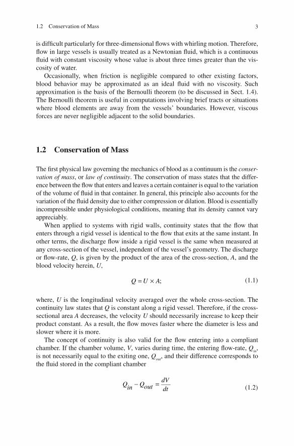
A compliant vessel is able to store part of the incoming fl uid during expansion. Therefore, the discharge is not constant along a vessel with elastic walls. The fl ow reduces downstream during vessel expansion and increases during contraction. This mechanism is used by compliant vessels to smooth out the sharp fl ow accelerations, accumulate the blood volume when the vessels expand and release volume during contraction. The law of continuity ( 1.2 ) states that the difference in the fl ow-rate between the two consecutive cross-sections must balance the change of the internal volume in that segment of the vessel. For example, the volume stored laterally in a segment with length L of an expanding vessel is Δ V = ∆ A × L , where ∆ A is the change in the vessel area. Continuity (Eq. 1.2 ) also states that the rate of change of volume dV / dt , which is equal to dA / dt × L balances the difference of the fl ow rate, ∆ Q , between the two ends of the vessel segment. As a result, the (negative) fl ow gradient along the vessel, ∆ Q / L , is balanced by the rate of expansion of the cross-sectional area of vessel, dA / dt (Fig. 1.2 ).

In general, by considering an arbitrarily brief segment, the fl ow gradient ∆ Q / L along the vessel is expressed by dQ / dx , and the law of continuity for the vessel describes as

0

∂ ∂∂ ∂

+ =Q A

x t (1.3)

Equation 1.3 shows how a sharp peak of fl ow decreases downstream ( dQ / dx < 0) along an elastic (compliant) vessel due to vessel expansion ( dA / dt > 0) based on a synchronous peak of pressure (Pedley 1980 , Sect. 2.1.1; Fung 1997 , Sect. 3.8).

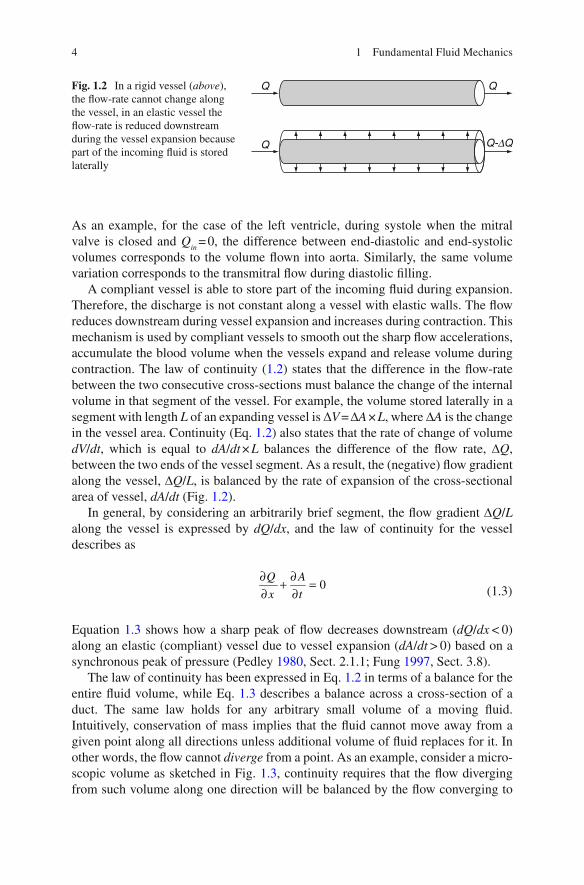
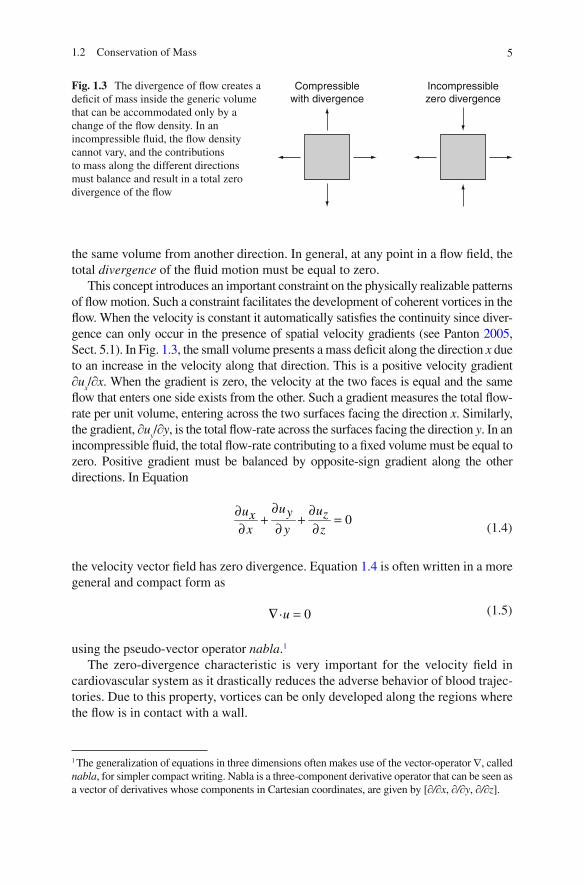
The law of continuity has been expressed in Eq. 1.2 in terms of a balance for the entire fl uid volume, while Eq. 1.3 describes a balance across a cross-section of a duct. The same law holds for any arbitrary small volume of a moving fl uid. Intuitively, conservation of mass implies that the fl uid cannot move away from a given point along all directions unless additional volume of fl uid replaces for it. In other words, the fl ow cannot diverge from a point. As an example, consider a micro-scopic volume as sketched in Fig. 1.3 , continuity requires that the fl ow diverging from such volume along one direction will be balanced by the fl ow converging to

Q

Q

Q

Q-DQ

Fig. 1.2 In a rigid vessel ( above ), the fl ow-rate cannot change along the vessel, in an elastic vessel the fl ow-rate is reduced downstream during the vessel expansion because part of the incoming fl uid is stored laterally


the same volume from another direction. In general, at any point in a fl ow fi eld, the total divergence of the fl uid motion must be equal to zero.

This concept introduces an important constraint on the physically realizable patterns of fl ow motion. Such a constraint facilitates the development of coherent vortices in the fl ow. When the velocity is constant it automatically satisfi es the continuity since diver-gence can only occur in the presence of spatial velocity gradients (see Panton 2005 , Sect. 5.1). In Fig. 1.3 , the small volume presents a mass defi cit along the direction x due to an increase in the velocity along that direction. This is a positive velocity gradient ∂u

x / ∂x . When the gradient is zero, the velocity at the two faces is equal and the same

fl ow that enters one side exists from the other. Such a gradient measures the total fl ow-rate per unit volume, entering across the two surfaces facing the direction x . Similarly, the gradient, ∂u

y / ∂y , is the total fl ow-rate across the surfaces facing the direction y . In an

incompressible fl uid, the total fl ow-rate contributing to a fi xed volume must be equal to zero. Positive gradient must be balanced by opposite-sign gradient along the other directions. In Equation

0

∂ ∂∂∂ ∂ ∂

+ + =u uu y zx

x y z (1.4)

the velocity vector fi eld has zero divergence. Equation 1.4 is often written in a more general and compact form as

· 0∇ =u (1.5)

using the pseudo-vector operator nabla . 1 The zero-divergence characteristic is very important for the velocity fi eld in

cardiovascular system as it drastically reduces the adverse behavior of blood trajec-tories. Due to this property, vortices can be only developed along the regions where the fl ow is in contact with a wall.

Compressiblewith divergence

Incompressiblezero divergence

Fig. 1.3 The divergence of fl ow creates a defi cit of mass inside the generic volume that can be accommodated only by a change of the fl ow density. In an incompressible fl uid, the fl ow density cannot vary, and the contributions to mass along the different directions must balance and result in a total zero divergence of the fl ow

1 The generalization of equations in three dimensions often makes use of the vector-operator Ñ, called nabla , for simpler compact writing. Nabla is a three-component derivative operator that can be seen as a vector of derivatives whose components in Cartesian coordinates, are given by [ ∂/∂x , ∂/∂y , ∂/∂z ].


1.3 Conservation of Momentum and Bernoulli Theorem

Momentum is a vector quantity equivalent to the product of the mass and the veloc-ity. The conservation of momentum states that the impulse of any system does not change unless an external force is applied to it. The conservation of momentum can be expressed for a fl uid by considering that a fl ow particle accelerates only when there is a pressure gradient applied to it. As sketched in Fig. 1.4 , a fl uid particle accelerates along a streamline when there is a negative pressure gradient along such a direction. Newton’s second law per unit volume of fl uid is shown here:

= − ∂

∂p

as

r (1.6)

where r is the fl uid density. However, the acceleration of a fl uid particle, a , is not a realistically measurable quantity since individual particles cannot be fol-lowed during their motion. Therefore, it is only feasible to deal with quantities measured at fi xed positions, rather than moving particles. As a result, the accelera-tion of a fl uid particle is expressed in terms of velocity space-time variations at fi xed positions.

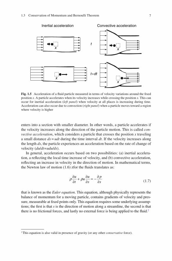
Let us consider a particle that instantaneously passes through a fi xed position x at the time t . With reference to Fig. 1.5 (left), consider a fl ow fi eld with velocity that is spatially uniform and increases only in time. The fl uid particles in this fi eld accelerate while they cross the position x as the velocity increases everywhere. This acceleration given by the local velocity time-derivative ∂u / ∂t is called inertial acceleration since it is associated with a change in the inertia of a volume of fl uid. A particle may also accelerate in a steady fl ow when the velocity is constant every-where in time, if it moves from a region of low-velocity toward a region where velocity is higher. The Fig. 1.5 (right) illustrates a particle that accelerates when

Negative pressure gradient(favourable, acceleration)

P P

P-DP P+DP

Positive pressure gradient(adverse, deceleration)

Fig. 1.4 A fl uid particle accelerates in presence of a negative pressure gradient ( left picture ) and decelerates in presence of an adverse pressure gradient

71.3 Conservation of Momentum and Bernoulli Theorem

enters into a section with smaller diameter. In other words, a particle accelerates if the velocity increases along the direction of the particle motion. This is called con-vective acceleration , which considers a particle that crosses the position x traveling a small distance ds = udt during the time interval dt . If the velocity increases along the length ds , the particle experiences an acceleration based on the rate of change of velocity ( du / dt =udu/ds).

In general, acceleration occurs based on two possibilities: (a) inertial accelera-tion, a refl ecting the local time increase of velocity, and (b) convective acceleration, refl ecting an increase in velocity in the direction of motion. In mathematical terms, the Newton law of motion (1.6) zfor the fl uids translates as:

+ = −∂ ∂ ∂

∂ ∂ ∂u u p

ut s s

r r (1.7)

that is known as the Euler equation. This equation, although physically represents the balance of momentum for a moving particle, contains gradients of velocity and pres-sure, measurable at fi xed points only. This equation requires some underlying assump-tions; the fi rst is that s is the direction of motion along a streamline, the second is that there is no frictional forces, and lastly no external force is being applied to the fl uid. 2

2 This equation is also valid in presence of gravity (or any other conservative force).

Inertial acceleration

x

xx

xt

t+dt

Convective acceleration

Fig. 1.5 Acceleration of a fl uid particle measured in terms of velocity variations around the fi xed position x . A particle accelerates when its velocity increases while crossing the position x . This can occur for inertial acceleration ( left panel ) when velocity at all places is increasing during time. Acceleration can also occur due to convection ( right panel ) when a particle moves toward a region where velocity is higher


The Bernoulli law is derived from the Euler equation. The Euler Eq. 1.7 can be rewritten in the alternate form of

( )21 02+ + =∂ ∂

∂ ∂u

u pt s

r r (1.8)

which shows that the variation in the total energy along a streamline is balanced by the change of fl uid inertia. Considering the integration rule for the sum of the varia-tions along a line, integration of Eq. 1.8 between two arbitrary points of 1 and 2 along a streamline gives:

2 22 2 1 1

21 12 2 1

+ = + − ∫∂∂u

u p u p dxt

r r r (1.9)

which is called the general Bernoulli equation . The Bernouli equation represents the conservation of mechanical energy given by the sum of the potential energy, p , and the kinetic energy, ½ r u 2 . The Bernoulli theorem states that variation of the mechanical energy from a point to another point along a streamline results in accel-eration or deceleration of the fl uid along that path, if there is no frictional (viscous) forces. The last term accounts for variation in the fl uid inertia.

When inertial effect is negligible, the Bernoulli theorem reduces to a special case of the conservation of energy, p + ½ r u 2 , along a streamline. The Bernoulli the-orem is often employed to measure the pressure drop from a large cardiac chamber (when u

1 is negligible), at peak systole or at peak diastole when the inertial term is

negligible. The same principle can be used for fl ow across the aortic valve or across a stenosis. In these cases, Eq. ( 1.9 ) simplifi es to

22

2 112− =p p ur

(1.10)

This formula is often utilized to obtain pressure from fl ow velocity, and if the veloc-ity is expressed in terms of m / s and pressure in terms of mmHg , then p

2 − p

1 = 4 u 2 .

The Bernoulli theorem represents the conservation of mechanical energy and allows evaluating the transformation of potential energy into kinetic energy and vice versa. It explains the underlying connection between variations in velocity and pres-sure. In its simplest form, fl ow that enters a stenotic segment increases its velocity due to conservation of mass and, because of the conservation of mechanical energy expressed by the Bernoulli theorem, reduces the pressure to balance the increase in kinetic energy.

In fact, the law of conservation of momentum implies that of conservation of energy and vice versa. In mechanics, momentum and energy balances are equivalent physical laws. The Euler equation ( 1.7 ) is an important simplifi ed form, which is

91.4 Conservation of Momentum and Viscosity

valid along a streamline only. For completeness, let us describe the three-dimensional Euler equation as:

·∇ ∇+ = −∂

∂u

u u pt

r r (1.11)

written in compact form using the operator Ñ, where the velocity, u , is a three-dimensional vector. The Euler equation ( 1.11 ) is either a vector equation or a system of three scalar equations along each coordinate. The Euler equation describes the motion of a fl uid under the fundamental assumption that any form of friction is neglected, thus it represents the conservation of mechanical energy, allowing trans-formations between different states with no energy loss. This equation is valid for ideal fl uids or inviscid fl ows in which the friction due to viscous phenomena can be neglected. These dissipative phenomena are considered in the next sections.

1.4 Conservation of Momentum and Viscosity

Viscosity is an intrinsic property of a fl uid that gives rise to the development of viscous shear stresses inside the fl ow. Energy dissipation due to viscous stresses is the only mechanism for energy loss in fl uids. In fact, the viscous friction phenom-enon transforms mechanical energy into thermal energy.

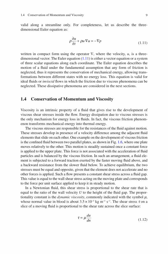
The viscous stresses are responsible for the resistances of the fl uid against motion. These stresses develop in presence of a velocity difference among the adjacent fl uid elements that slide on each other. One example on the development of viscous friction is the confi ned fl uid between two parallel plates, as shown in Fig. 1.6 , where one plate moves relatively to the other. This motion is steadily sustained once a constant force is applied to the upper plate. This force is not associated with the acceleration of fl uid particles and is balanced by the viscous friction. In such an arrangement, a fl uid ele-ment is subjected to a forward traction exerted by the faster moving fl uid above, and a backward resistance from the slower fl uid below. To achieve equilibrium, the two stresses must be equal and opposite, given that the element does not accelerate and no other forces is applied. Such a fl ow presents a constant shear stress across a fl uid gap. This value is equal to the wall shear stress acting on the moving plate and corresponds to the force per unit surface applied to keep it in steady motion.

In a Newtonian fl uid, this shear stress is proportional to the shear rate that is equal to the ratio of the wall velocity U to the height of the fl uid gap. The propor-tionality constant is the dynamic viscosity , commonly indicated with the symbol m , whose normal value in blood is about 3.5 × 10 −3 kg m −1 s −1 . The shear stress t on a slice of a moving fl uid is proportional to the shear rate across the slice surface:

= du

dnt m

(1.12)


In a non-Newtonian fl uid, the viscosity is not constant and depends on the local state of shear rate of the fl uid elements. However, as previously discussed in Sect. 1.1, non-Newtonian effects are typically negligible in large vessels due to the dominance of the inertia in that setting. As a result, the non-Newtonian corrections do not sig-nifi cantly affect the analysis involved in vortex dynamics.

Newtonian viscous stresses can be immediately accounted for the motion along a streamline. When shear stress is constant across a streamline, a forward shear stress acts on that streamline from above and an identical backward stress acts from below with no net force (Fig. 1.6 ). In general (e.g. Fig. 1.4), the motion of the fl uid particle is subjected to a shear stress on one side and another shear stress on the opposite side with a negative sign. The total viscous force, per unit volume, is thus due to the variation of the shear stress across the streamline, in formulas ( ∂ t / ∂n ), where n indicates the direction across that streamline. This viscous force can be described in terms of the velocity, m ∂ 2 u / ∂n 2 , based on Eq. 1.12 . Considering the viscous forces in the equation of motion, it transforms the Euler equation into the Navier-Stokes equation:

2

2+ = − +t

∂ ∂ ∂ ∂∂ ∂ ∂ ∂u u p u

us s n

r r m (1.13)

The two equations differ by the viscous term only. 3 This term is not easy to evaluate in most fl ow conditions, and often neglected when applying the Bernoulli balance. However, in three-dimensional fl ow, the viscous term must be properly accounted for all gradients of shear stress across a point. As a result, the three-dimensional Navier-Stokes equation describes as (see Panton 2005 , Sects. 6.2 and 6.6):

21·∇ ∇ ∇+ = − +∂ ν

∂u

u u p ut r (1.14)

U+t

−t

Fig. 1.6 When the upper plate is in motion with velocity U relative to the fi xed plate below, shear stress is constant across the gap between the two plates because every fl uid element is in equilib-rium subjected to the shear forces given by the faster fl uid above and the slower fl uid below. In a Newtonian fl uid, the velocity grows linearly from zero adjacent to the bottom plate to U at the upper plate

3 This intuitive result is somehow simplifi ed: the viscous term should include variations along all directions about the streamline. In particular for three-dimensional fl ow, it should include the other direction perpendicular to both the streamline and to n . It was simplifi ed here to avoid unnecessary symbolic complications.

111.5 Boundary Layer and Wall Shear Stress

This fundamental equation describes all aspects of the fl uid motion, under the assumption of incompressible, Newtonian fl uid, in the absence of non-conservative forces. The kinematic viscosity n , which is introduced in Eq. 1.14 is given by the ratio of the dynamic viscosity to the fl uid density, n = m / r , and its value for blood is about 3.3 × 10 −6 m 2 /s (or 3.3 mm 2 /s). The kinematic viscosity is a more common viscous coeffi cient when dealing with blood motion, including vortex dynamics, because incompressible motion is independent of the actual value of density. This is a value that enters into play only as a multiplicative factor when motion is quantifi ed in terms of force, work, or energy.

The kinematic viscosity is a small coeffi cient by itself. Therefore, for the viscous term to show signifi cant effect, presence of sharp velocity gradients are required. Indeed, viscous effects are often negligible with respect to potential-kinetic energy transformation along brief paths (e.g. when the Bernoulli equation is used). Alternatively, dissipation is going to have signifi cant effect once summed up over long fl uid paths and for circulation balances.

Presence of viscosity introduces a fundamental novel element to fl uid dynamics. Viscosity implies the continuity of motion between adjacent slices that smoothly slide over each other due to the gradient of velocity. However, they cannot present a net velocity difference otherwise the shear rate and the viscous term would rise to infi nity. This continuity also applies to the fi rst fl uid elements adjacent to a solid boundary, where it implies the adherence between the fl uid and structure. This con-dition, normally referred as no-slip condition , is a result of viscosity and does not apply in an ideal fl uid.

1.5 Boundary Layer and Wall Shear Stress

The adherence of fl uid at the solid boundaries is a purely viscous phenomenon, which implies that the viscous effects can never be neglected close to the walls. Near the solid boundary, a layer of fl uid exists whose motion is directly infl uenced by the adherence to the boundary. This infl uence of wall on the fl uid is gradually reduced, and sometimes even disappears once moving away from the boundary toward the bulk fl ow. The boundary layer is the region where velocity rapidly grows from a zero value at the wall to reach values comparable to those found at the center of the vessel. The wall shear stress , t

w , is the stress exerted by the fl uid over the

endothelial layer, and is proportional to the wall shear rate, which is the gradient of velocity at the wall. This value is approximately the ratio of the fl uid velocity away from the wall, U , to the boundary layer thickness, commonly indicated as d :

= ≈

δdu U

w dn wallt m m

(1.15)

The higher the fl uid velocity is, the higher the wall shear stress will be. Additionally, a thinner boundary layer results in higher wall shear stress.


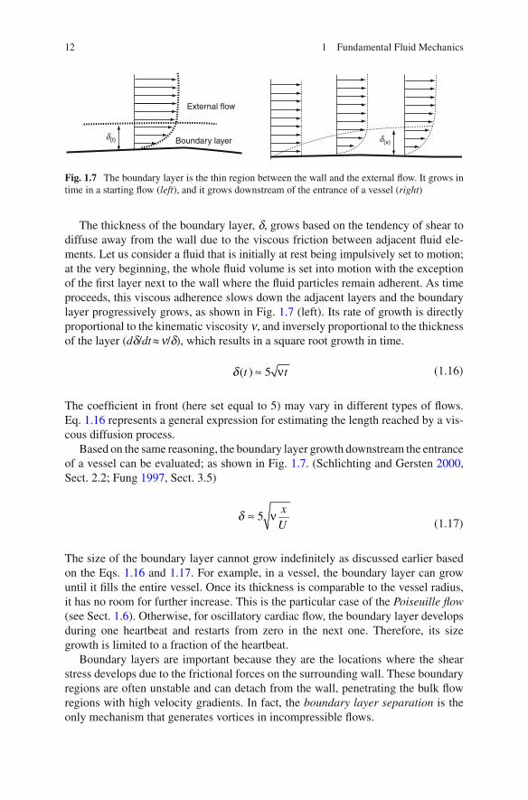
The thickness of the boundary layer, d , grows based on the tendency of shear to diffuse away from the wall due to the viscous friction between adjacent fl uid ele-ments. Let us consider a fl uid that is initially at rest being impulsively set to motion; at the very beginning, the whole fl uid volume is set into motion with the exception of the fi rst layer next to the wall where the fl uid particles remain adherent. As time proceeds, this viscous adherence slows down the adjacent layers and the boundary layer progressively grows, as shown in Fig. 1.7 (left). Its rate of growth is directly proportional to the kinematic viscosity n , and inversely proportional to the thickness of the layer ( d d / dt » n / d ), which results in a square root growth in time.

( ) 5≈ νt td (1.16)

The coeffi cient in front (here set equal to 5) may vary in different types of fl ows. Eq. 1.16 represents a general expression for estimating the length reached by a vis-cous diffusion process.

Based on the same reasoning, the boundary layer growth downstream the entrance of a vessel can be evaluated; as shown in Fig. 1.7 . (Schlichting and Gersten 2000 , Sect. 2.2; Fung 1997 , Sect. 3.5)

5≈ ν x

Ud

(1.17)

The size of the boundary layer cannot grow indefi nitely as discussed earlier based on the Eqs. 1.16 and 1.17 . For example, in a vessel, the boundary layer can grow until it fi lls the entire vessel. Once its thickness is comparable to the vessel radius, it has no room for further increase. This is the particular case of the Poiseuille fl ow (see Sect. 1.6 ). Otherwise, for oscillatory cardiac fl ow, the boundary layer develops during one heartbeat and restarts from zero in the next one. Therefore, its size growth is limited to a fraction of the heartbeat.

Boundary layers are important because they are the locations where the shear stress develops due to the frictional forces on the surrounding wall. These boundary regions are often unstable and can detach from the wall, penetrating the bulk fl ow regions with high velocity gradients. In fact, the boundary layer separation is the only mechanism that generates vortices in incompressible fl ows.

Boundary layer

External flow

d(t) d(x)

Fig. 1.7 The boundary layer is the thin region between the wall and the external fl ow. It grows in time in a starting fl ow ( left ), and it grows downstream of the entrance of a vessel ( right )

131.6 Simple Flows and Concepts of Cardiovascular Interest


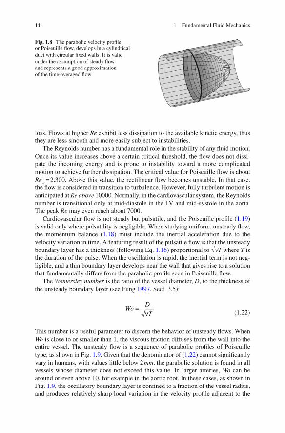
A simple but important type of fl ow motion is a fl ow inside a cylindrical vessel with circular cross-section. Considering that the fl ow is steady and uniform, both inertial and convective accelerations are zero (see Eq. 1.13 ). To be more precise, a cylinder of fl uid with unit length and radius r is pushed ahead by the negative pressure gradi-ent dp / dx acting on the cross-sectional area p r 2 , and is subjected to the shear stress t = m du / dr on the lateral surface 2 p r . These two forces must balance to ensure equi-librium. Therefore:

2=du r dp

dr dxm (1.18)

where the pressure gradient is constant over the cross-section because no cross-fl ow exists. The Eq. 1.18 is satisfi ed by a parabolic velocity profi le u ( r ) that ensures the adher-ence condition at the vessel wall (Fig. 1.8 ). Assuming a vessel with radius R , the solution is

( ) ( )2 2 2 2

2

1 2( )

4−= − = −dp U

u r R r R rdx Rm (1.19)

Equation 1.19 is the well-known Poiseuille fl ow (see Schlichting and Gersten 2000 , Sect. 5.2.1; Fung 1997 , Sect. 3.2). The Poiseuille fl ow can be equivalently expressed in terms of the pressure gradient or the mean velocity U ( second equality in Eq. 1.19 ), that are related based on dp / dx = − 8 m U / R 2 verifi able by taking an integral from Eq. 1.19 . It features a maximum velocity at the center that is twice the average velocity, and a wall shear stress of 4 m U / R . Pressure loss, − dp / dx , is usually expressed with respect to the kinetic energy, ½ r U 2 , per unit diameter length, D = 2 R of the tube. The friction factor , l , is described as:

2

2−= D dpU dx

lr (1.20)

that is a dimensionless quantity suitable for generalization under different condi-tions. In the Poiseuille fl ow, the friction factor is given by 64/ Re where the Reynolds number is

=

νUD

Re (1.21)

and represents the ratio of inertial to viscous forces in the fl uid. Flows with low values of the Reynolds numbers are highly viscous, smooth, with high pressure-


loss. Flows at higher Re exhibit less dissipation to the available kinetic energy, thus they are less smooth and more easily subject to instabilities.

The Reynolds number has a fundamental role in the stability of any fl uid motion. Once its value increases above a certain critical threshold, the fl ow does not dissi-pate the incoming energy and is prone to instability toward a more complicated motion to achieve further dissipation. The critical value for Poiseuille fl ow is about Re

cr = 2,300. Above this value, the rectilinear fl ow becomes unstable. In that case,

the fl ow is considered in transition to turbulence. However, fully turbulent motion is anticipated at Re above 10000. Normally, in the cardiovascular system, the Reynolds number is transitional only at mid-diastole in the LV and mid-systole in the aorta. The peak Re may even reach about 7000.

Cardiovascular fl ow is not steady but pulsatile, and the Poiseuille profi le ( 1.19 ) is valid only where pulsatility is negligible. When studying uniform, unsteady fl ow, the momentum balance ( 1.18 ) must include the inertial acceleration due to the velocity variation in time. A featuring result of the pulsatile fl ow is that the unsteady boundary layer has a thickness (following Eq. 1.16 ) proportional to √ n T where T is the duration of the pulse. When the oscillation is rapid, the inertial term is not neg-ligible, and a thin boundary layer develops near the wall that gives rise to a solution that fundamentally differs from the parabolic profi le seen in Poiseuille fl ow.

The Womersley number is the ratio of the vessel diameter, D , to the thickness of the unsteady boundary layer (see Fung 1997 , Sect. 3.5):

=

νD

WoT (1.22)

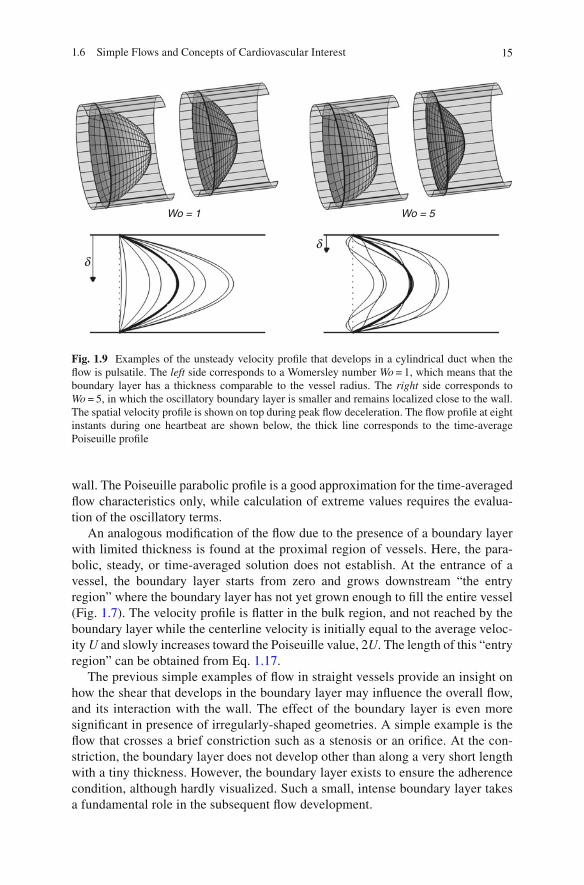
This number is a useful parameter to discern the behavior of unsteady fl ows. When Wo is close to or smaller than 1, the viscous friction diffuses from the wall into the entire vessel. The unsteady fl ow is a sequence of parabolic profi les of Poiseuille type, as shown in Fig. 1.9 . Given that the denominator of ( 1.22 ) cannot signifi cantly vary in humans, with values little below 2 mm , the parabolic solution is found in all vessels whose diameter does not exceed this value. In larger arteries, Wo can be around or even above 10, for example in the aortic root. In these cases, as shown in Fig. 1.9 , the oscillatory boundary layer is confi ned to a fraction of the vessel radius, and produces relatively sharp local variation in the velocity profi le adjacent to the

Fig. 1.8 The parabolic velocity profi le or Poiseuille fl ow, develops in a cylindrical duct with circular fi xed walls. It is valid under the assumption of steady fl ow and represents a good approximation of the time-averaged fl ow


wall. The Poiseuille parabolic profi le is a good approximation for the time-averaged fl ow characteristics only, while calculation of extreme values requires the evalua-tion of the oscillatory terms.

An analogous modifi cation of the fl ow due to the presence of a boundary layer with limited thickness is found at the proximal region of vessels. Here, the para-bolic, steady, or time-averaged solution does not establish. At the entrance of a vessel, the boundary layer starts from zero and grows downstream “the entry region” where the boundary layer has not yet grown enough to fi ll the entire vessel (Fig. 1.7 ). The velocity profi le is fl atter in the bulk region, and not reached by the boundary layer while the centerline velocity is initially equal to the average veloc-ity U and slowly increases toward the Poiseuille value, 2 U . The length of this “entry region” can be obtained from Eq. 1.17 .

The previous simple examples of fl ow in straight vessels provide an insight on how the shear that develops in the boundary layer may infl uence the overall fl ow, and its interaction with the wall. The effect of the boundary layer is even more signifi cant in presence of irregularly-shaped geometries. A simple example is the fl ow that crosses a brief constriction such as a stenosis or an orifi ce. At the con-striction, the boundary layer does not develop other than along a very short length with a tiny thickness. However, the boundary layer exists to ensure the adherence condition, although hardly visualized. Such a small, intense boundary layer takes a fundamental role in the subsequent fl ow development.

dd

Wo = 1 Wo = 5

Fig. 1.9 Examples of the unsteady velocity profi le that develops in a cylindrical duct when the fl ow is pulsatile. The left side corresponds to a Womersley number Wo = 1, which means that the boundary layer has a thickness comparable to the vessel radius. The right side corresponds to Wo = 5, in which the oscillatory boundary layer is smaller and remains localized close to the wall. The spatial velocity profi le is shown on top during peak fl ow deceleration. The fl ow profi le at eight instants during one heartbeat are shown below, the thick line corresponds to the time-average Poiseuille profi le


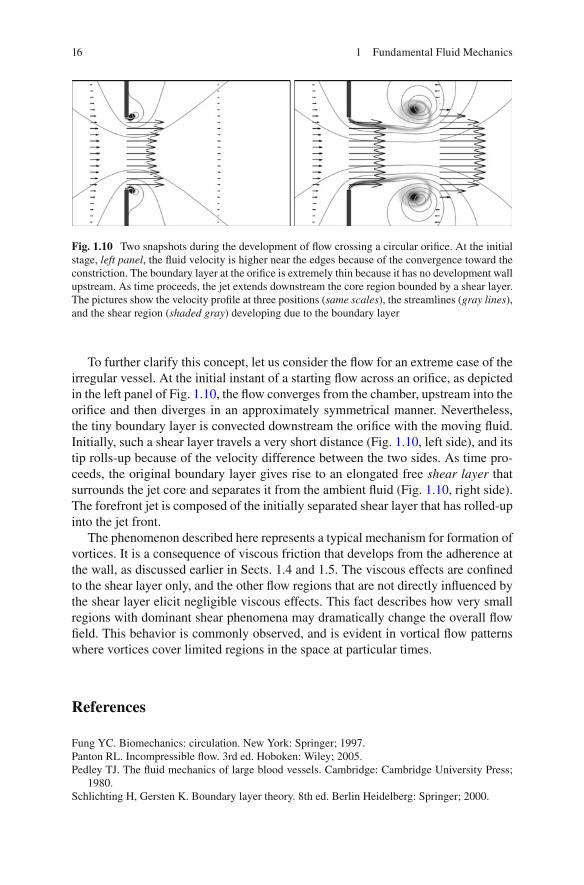
To further clarify this concept, let us consider the fl ow for an extreme case of the irregular vessel. At the initial instant of a starting fl ow across an orifi ce, as depicted in the left panel of Fig. 1.10 , the fl ow converges from the chamber, upstream into the orifi ce and then diverges in an approximately symmetrical manner. Nevertheless, the tiny boundary layer is convected downstream the orifi ce with the moving fl uid. Initially, such a shear layer travels a very short distance (Fig. 1.10 , left side), and its tip rolls-up because of the velocity difference between the two sides. As time pro-ceeds, the original boundary layer gives rise to an elongated free shear layer that surrounds the jet core and separates it from the ambient fl uid (Fig. 1.10 , right side). The forefront jet is composed of the initially separated shear layer that has rolled-up into the jet front.

The phenomenon described here represents a typical mechanism for formation of vortices. It is a consequence of viscous friction that develops from the adherence at the wall, as discussed earlier in Sects. 1.4 and 1.5. The viscous effects are confi ned to the shear layer only, and the other fl ow regions that are not directly infl uenced by the shear layer elicit negligible viscous effects. This fact describes how very small regions with dominant shear phenomena may dramatically change the overall fl ow fi eld. This behavior is commonly observed, and is evident in vortical fl ow patterns where vortices cover limited regions in the space at particular times.

References

Fung YC. Biomechanics: circulation. New York: Springer; 1997. Panton RL. Incompressible fl ow. 3rd ed. Hoboken: Wiley; 2005. Pedley TJ. The fl uid mechanics of large blood vessels. Cambridge: Cambridge University Press;

1980. Schlichting H, Gersten K. Boundary layer theory. 8th ed. Berlin Heidelberg: Springer; 2000.

Fig. 1.10 Two snapshots during the development of fl ow crossing a circular orifi ce. At the initial stage, left panel , the fl uid velocity is higher near the edges because of the convergence toward the constriction. The boundary layer at the orifi ce is extremely thin because it has no development wall upstream. As time proceeds, the jet extends downstream the core region bounded by a shear layer. The pictures show the velocity profi le at three positions ( same scales ), the streamlines ( gray lines ), and the shear region ( shaded gray ) developing due to the boundary layer

fundamental fluid mechanics - units.it · 2016-09-14 · 4 1 fundamental fluid mechanics as an...

Documents