fundamental economic structure and structural change...

___________________ Région et Développement n° 33-2011 __________________

FUNDAMENTAL ECONOMIC STRUCTURE AND STRUCTURAL CHANGE IN REGIONAL ECONOMIES:

A METHODOLOGICAL APPROACH

Sudhir K. THAKUR

Abstract: Regional economic structure is defined as the composition and patterns of various components of the regional economy such as: produc-tion, employment, consumption, trade, and gross regional product. Structur-al change is conceptualized as the change in relative importance of the aggregate indicators of the economy. The process of regional development and structural change are intertwined, implying as economic development takes place the strength and direction of intersectoral relationships change leading to shifts in the importance, direction and interaction of economic sectors such as: primary, secondary, tertiary, quaternary and quinary sec-tors. The fundamental economic structure (FES) concept implies that selected characteristics of an economy will vary predictably with region size. The identification of FES leads to an improved understanding of the space-time evolution of regional economic activities at different geograph-ical scales. The FES based economic activities are predictable, stable and important. This paper reviews selected themes in manifesting an improved understanding of the relationship among intersectoral transactions and economic size leading to the identification of FES. The following four ques-tions are addressed in this paper: (1) What are the relationships among sector composition and structural change in the process of economic devel-opment? (2) What are the approaches utilized to study structural change analysis? (3) Can a methodology be developed to identify FES for regional economies? (4) Would the identification of FES manifest an improved con-ception of the taxonomy of economies? Keywords: STRUCTURAL CHANGE AND FUNDAMENTAL ECONOMIC STRUCTURE. JEL Classification: DF7, O11, R11

College of Business Administration, California State University Sacramento. [email protected]

10 Sudhir K. Thakur

1. INTRODUCTION

Economic structure is defined as the composition of various components of the macro aggregates, relative change in their size over time, and its relation-ship with the circular flow of income (Jackson et al., 1990). As regional econo-mies develop from an agricultural, to industrialized and service-sector (quater-nary and quinary sectors) based economies there is an explicit transformation among the intersectoral relationships among industries. The initial concentration of economic interaction is among primary sector activities, and matures to sec-ondary and tertiary sector interaction at later stages of development. Given this perspective the overarching question addressed in this paper is whether there are identifiable patterns of relationships among economic transactions and macroe-conomic aggregates as revealed by input-output tables. Would identification of such patterns allow regional analysts to predict regional change in a statistical sense? What is the methodology to identify fundamental economic structure (FES)?

Shishido et al. (2000) studied twenty countries from Asian economies and concluded that if the input coefficients in the Leontief table are partitioned into „principal‟, „supporting‟ and „primary‟ groups, then the second and third groups would in all likelihood change as the economy develops. The first group showed no change in pattern with economic development while the latter two showed changes. This suggests the existence of a fundamental component in the regional economic structure. FES represents those economic activities that are consistently present in regional economies of varying size and complexity with-in a nation. The compilation of input-output table is manpower intensive, ex-pensive and time consuming. If a component of the transaction matrix can be predicted using FES it will save resources in compiling national and regional tables.

A survey of structural change analysis has discovered that studies in the relationship linking technical change and economic growth have gained signifi-cance during the 1990s (Silva and Teixeira, 2008). Holland and Cooke (1992) analyzed the regional tables for Washington economy and concluded that changes in output especially in the service sector were driven by international demand. Jensen et al. (1988) and West (2000) utilized a fundamental economic structure (FES) approach to identify predictable cells in the regional tables for Australia. Thakur (2008 and 2010) identified a temporal and a regional FES for the Indian economy. The analysis suggests the existence of FES at different geographical scales. Also, these economic structures are predictable, stable and important. The identification of fundamental cells was based on the assumption that regions exhibited a predictable pattern based on the similarities in regional economies across space and time. The FES approach has been an important milestone in identifying the engines of regional growth. The framework has been utilized to predict the regional tables for economies utilizing times-series and cross-section data on economic structure (West 2000 and 2001).

As economic development takes place the nature of interaction among economic sectors undergoes transformation. Jackson et al. (1989) posit a rela-

Région et Développement 11

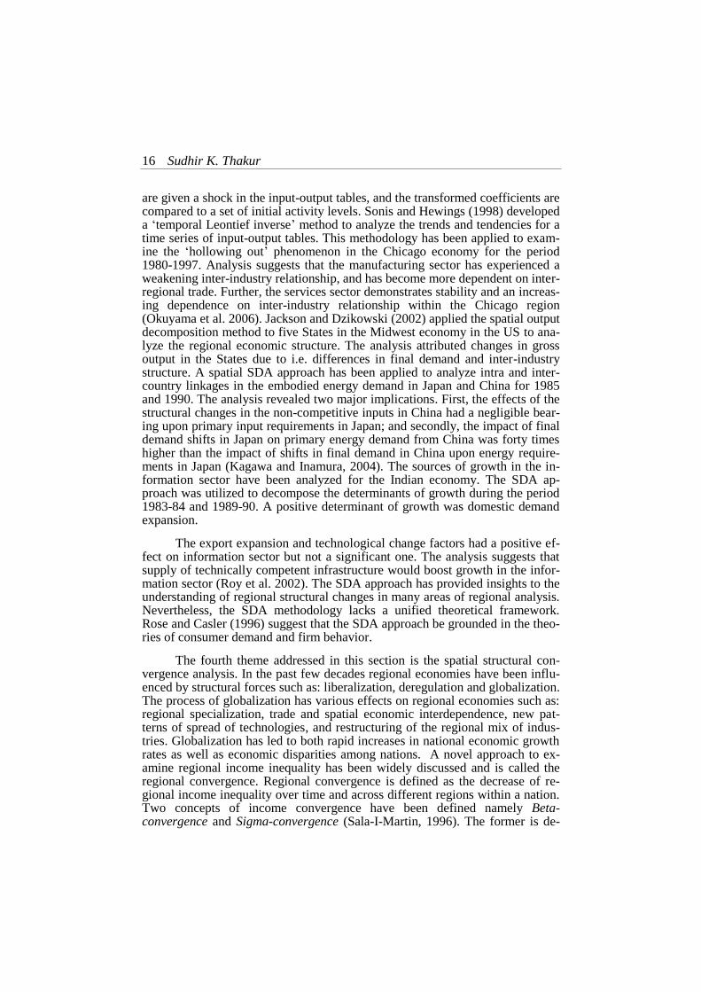
tionship between stages in economic development associated with sector inter-action. They argued that as an economy expands from a primary stage to a more complex stage, the relationship between sector linkages and economic devel-opment becomes intricate. In the initial stage, the regional economy‟s interde-pendence increases gradually and, later, it increases at faster pace, leading to a strong interaction among sectors. Thus, economies will be strongly dependent on the primary sector and as secondary sector activities are introduced, interac-tion propagates among the two sectors. The industrial restructuring process introduces service sectors such as: finance, insurance, high technology and trade sectors which predominate. At a mature stage of development, slowing in, the pace of inter-industry interactions are expected, leading to a maximum with the possibility of a decline in interactions known as the process of „hollowing out‟ (Figure 1). This process has been observed in the Japanese economy where the employment in the manufacturing sector has significantly declined, and in-creased in the service-sector, followed by an increase in the share of foreign direct investment by Japanese firms in foreign locations (Prasad, 1997).

Figure 1: Regional Economic Development Process

Source: Hewings, Jensen and West (1988).

Likewise, the Chicago economy has shown a hollowing out as well with

the implication that intra-metropolitan dependence in economic interaction has declined and dependence on sources of supply and demand on outside the re-gion has increased (Hewings et al. 1988a; Hewings et al. 1998). Also, the Tai-wanese economy has shown a decline in the density of inter-sector linkages since the beginning of the 1980s (West and Brown, 2003). An important aspect of development debate since the early twentieth century has been the identifica-tion of regularities, patterns and common trends in the process of development.

Significant Changes

in Transactions

Few Interactions

Possible Hollowing

Out

Almost Mature

Mature and Most Complex

Complexity

Time

12 Sudhir K. Thakur

A significant element in this endeavor has been to understand the relationship between economic development and structural change in the process of modern-ization.

This paper is organized into five sections: the second section examines selected themes to shed light on the relationships among sector composition, structural change and economic development; the third section discusses the applications of selected methods of structural change followed by the fourth section which outlines the quantitative methodology of the identification of FES; and the last section concludes.

2. ECONOMIC STRUCTURE, STRUCTURAL CHANGE AND DEVELOPMENT

The „structural complexity‟ of an economic system can be understood by decomposing an economy into three elements: „structure‟, „processes‟, and pro-cess explaining „complexity‟ in the economy (Pryor, 1996). Structure is defined as the composition and patterns of components of the macro-economic aggre-gates. Process involves both description and analysis to identify structural change within economies. A glance at the indicators of structural change will portray a snapshot of the patterns of change occurring in an economy at a given point in time and space. The analytic task is that of exploring the mechanism producing change. Thus, „structural changes‟ are modifications in relative im-portance of aggregative indicators of the economy. „Structural economic dy-namics‟ are the processes of time and space dependent changes and the inter-relationship between economic aggregates, such as: consumption, savings, in-vestment, and expenditure. Complexity deals with linking particular aspects of the behavior of the economic system with the structural components of the en-tire economic system (Pryor, 1996).

The process of economic development is explained by the shifting distri-bution of economic activities in a nation over space and time. To understand the distribution of economic activities three sectors are identified: primary, second-ary and tertiary, and a fourth category, quaternary sector can be added (Ke-nessey, 1987; Malecki, 1991). These sectors correspond to the assemblage of economic activities anchored in various production processes like: „extraction‟, „processing‟, „delivery‟ and „information‟ (Kenessey, 1987). Kenessey (1987) argues for a sectoral-structural hypothesis whereby primary, secondary, tertiary and quaternary activities can be broadly in equilibrium at different rates of growth and economic performance levels for the nation as a whole. To under-stand the growth momentum of these sectors an understanding of the linkages among these sectors is indispensable. If we assume an economy with three sec-tors: agriculture, industry and tertiary, there are nine permutations in which three sectors can interact leading to inter-sector interactions. Further, if we ab-stract from the various linkages and just examine the agriculture and industry linkage, then, this linkage can be traced through the role of agriculture as: (1) supplier of wage goods, mainly food grains to the industry sector, (2) provider of raw materials for agro-based industry, (3) generator of agricultural incomes which creates final demand for the output of the industrial sector, and (4) gener-


ator of demand for purchased inputs like fertilizers and pesticides for agricultur-al production. While the first two linkages represent supply side or backward linkages, the last two represent demand or forward linkage.

The early research by Chenery (1960) and Chenery and Taylor (1968) identified a pattern amongst large countries, small primary-oriented and small industry-oriented countries. They identified uniform patterns of change in the structure of production as the income level of nations rose. Chenery (1960) argued for uniform patterns in industrial growth since demand and supply fac-tors were analogous amongst countries and differences in growth would arise only due to differences in factor prices. In particular the role of technological change in the primary production, chemicals and metal products sectors were reinforced both at the cross-sectional and temporal levels. For instance, in the United States, industries in general shifted to larger consumption of services, electric energy, chemicals and synthetics, thus substituting for coal, wood and metals during the period 1958-62 (Carter, 1967). A cross-sectional study of 26 countries at various income levels have shown that intersectoral relationships have an „asymmetric dependence‟ of the service sector upon skill intensive and technologically dependent manufacturing activities (Park and Chan, 1989). In general, development patterns are not invariant over time and especially „tech-nological change‟ has a strong role in influencing structural change patterns across countries (Syrquin and Chenery, 1989).

There has been a great deal of interest in linking the association among

economic structure, development and structural transformation across inter-country and sub-national economies. The central argument is that nations begin as primary producers, then, resources shift to secondary production and, finally, to service production and these stages identify with the stages of development of economies. Several scholars, such as Chenery (1960), Chenery and Taylor (1968), Chenery (1979), Syrquin and Chenery (1989), identified „common or universal patterns of development‟ in their cross-sectional and longitudinal studies across nations and regional economies. The identified development pat-terns represented an expected milieu of change as economies transform from a low income agricultural economy to a high income urban-industrial economy (Pandit, 1991). This theme has also been investigated to identify shifts in labor shares across sectors as economic development takes place.

Clark (1940) and Fisher (1939) posit with rising levels of economic de-velopment, a decline in the share of labor in the agriculture sector is noticed, followed by an initial rise and subsequent decline in the industrial labor share. These two processes are followed by a monotonic increase in the share of labor in the tertiary sector. Pandit (1990a) observed a lacuna in the Fisher (1939), Clark (1940), and Chenery (1975) observations and postulated that the more recent developing countries had a higher share of labor force in the service sec-tor as opposed to the less recently developed countries. A „hump‟ is observed in a cross-sectional study of several countries though on an individual basis a ris-ing share of labor in the tertiary sector is observed. Katouzian (1970) suggested that this was true due to aggregation in the service sector since there was a great

14 Sudhir K. Thakur

deal of heterogeneity in the composition of service sector. The tertiary sector constituted three parts: „new services‟ with high income elasticity of demand, „old services‟ with low income elasticity of demand and „complementary ser-vices‟ those whose growth was linked with manufacturing sector in addition to government activities.

A tertiary sector hypertrophy (Pandit, 1990b) has been observed, though there is considerable spatial variation among world regions in this phenomenon. Several factors explain this trend. First, a surplus of urban labor supply exists in relation to manufacturing demand in many developing economies; second, rapid urbanization has led to an increasing demand of low-cost services; and third, the government has not operated the labor market efficiently. Pandit et al. (1989) and Pandit (1992) observed a „temporal drift‟ in sector-shift models among the developed and developing countries, suggesting a lack of regularity in the labor sector allocation as development occurs. Further, Pandit (1986) noted the im-pact of trading activities upon the labor force transformation among developing economies. In a nutshell, though the Clark-Fisher thesis is theoretically appeal-ing and provides a strong rationale for explaining the allocation of labor force across sectors, but, the notion can be acceptable only by examining its sensitivi-ty to temporal, spatial and contextual validity to shifts of labor force across sec-tors, and the shift of the sectors themselves (Casetti and Pandit, 1987).

3. METHODS OF STUDYING STRUCTURAL CHANGE

Regional analysts have developed several methodologies to measure, in-terpret and understand structural change. This section discusses four selected themes of the approaches utilized in measuring structural change. These meth-odologies manifest an improved understanding of the relationship among sector composition, structural change and economic development. These themes are: „identification of key sectors‟, „sector composition and economic growth‟, „structural decomposition analyses‟, and „spatial structural convergence‟.

The first theme examined is the key sector analysis. These are those sec-

tors within a regional economy that exercises their influence via sale and pur-chase relations, and is expected to have a more than average impact on the economy. Rasmussen (1957) proposed two indices that are widely used as measures for the identification of key sectors and these are: „power of disper-sion‟, and „sensitivity of dispersion‟. The power of dispersion is defined as the ratio of the average direct and indirect coefficient from column j to the average direct and indirect coefficient in the regional table. This implies if the ratio is larger than 1, a unit increase in the final demand for the column industry will translate into a greater than average change in activity in the economy. The sensitivity of dispersion measure is defined as the averages of the direct and indirect coefficients from row i to the average direct and indirect coefficient of the regional table. This implies if the final demand increases by 1 unit, the row will experience a more than an average impact on economic activities (Jackson, 1993). The identification of key sectors can be examined by the application of


alternative methodologies such as field of influence and identification of the minimum product matrix (MPM).

Hewings et al. (1989) in their analysis of the Brazilian economy exam-ined the identification of key sectors using the field of influence approach. They decomposed the inter-industry transaction into a hierarchy of flows and the flows associated with the higher levels of hierarchy were identified as key sec-tors. A new perspective of the identification of key sectors has been proposed by Sonis et al. (2000) based on a minimum information approach. Utilizing the Chinese input-output tables for 1987 and 1990 the regional economic structure has been decomposed into two components. The first component is extracted based upon the row and column multipliers from the Leontief inverse matrix. The second component is compiled from the synergetic interaction among sev-eral sectors of the regional economy. A multiplier product matrix (MPM) is then collated which depicts the economic landscape associated with the regional economic structure. However, these measures of economic structure are not devoid of limitations. The development process proposes multiple objectives to attain higher levels of employment, income, output, exports, and foreign ex-change; the identification of a few key sectors with a concentrated investment in such sectors cannot achieve the stated multiple objectives (Sonis et al. 1995).

The second theme seeks to identify statistically universal relationships between economic growth and change in economic structure using cross-section data or time-series data for national and sub-national economies. Kuznets (1966) in a sample of 24 countries and Chenery (1975) with a sample of 100 national economies showed how nations shared common patterns of structural change in the process of economic growth, and, thus, attempted to provide a general theory of structural change. This theme attempts to provide an under-standing of the process of historical change and experience as economies with similar initial conditions developed in time. Some of the theories used to ex-plain the process of structural change are the dual sector theory, Myint‟s vent for surplus theory (1958), and Todaro‟s rural-urban migration (1969). Also, Syrquin (1988) identifies three stages of structural transformation: first, primary production where the economy is characterized by low to moderate rates of capital accumulation, a fast increase in labor force and very low growth in total factor productivity; second, a shift towards the manufacturing sector contrib-uting more to growth, and third, a decline in the share of labor force in manu-facturing and an increase in export shares of manufactured goods, with an in-crease in the service sector. The shift from agriculture to industry sector can be explained by the decline in labor force and operation of Engel‟s law that leads to the decline of primary sector; a rise in the income elasticity of manufacturing goods; and a subsequent rise of income elasticity in the service sector in the third stage. This stage model is a general model linking sector linkage with eco-nomic development which may show discontinuities in different countries with respect to timing and scale.

The third methodology is the application of structural decomposition analysis (SDA) to understand sources of development and change in regional economies. SDA is a comparative static exercise in which sets of coefficients

16 Sudhir K. Thakur

are given a shock in the input-output tables, and the transformed coefficients are compared to a set of initial activity levels. Sonis and Hewings (1998) developed a „temporal Leontief inverse‟ method to analyze the trends and tendencies for a time series of input-output tables. This methodology has been applied to exam-ine the „hollowing out‟ phenomenon in the Chicago economy for the period 1980-1997. Analysis suggests that the manufacturing sector has experienced a weakening inter-industry relationship, and has become more dependent on inter-regional trade. Further, the services sector demonstrates stability and an increas-ing dependence on inter-industry relationship within the Chicago region (Okuyama et al. 2006). Jackson and Dzikowski (2002) applied the spatial output decomposition method to five States in the Midwest economy in the US to ana-lyze the regional economic structure. The analysis attributed changes in gross output in the States due to i.e. differences in final demand and inter-industry structure. A spatial SDA approach has been applied to analyze intra and inter-country linkages in the embodied energy demand in Japan and China for 1985 and 1990. The analysis revealed two major implications. First, the effects of the structural changes in the non-competitive inputs in China had a negligible bear-ing upon primary input requirements in Japan; and secondly, the impact of final demand shifts in Japan on primary energy demand from China was forty times higher than the impact of shifts in final demand in China upon energy require-ments in Japan (Kagawa and Inamura, 2004). The sources of growth in the in-formation sector have been analyzed for the Indian economy. The SDA ap-proach was utilized to decompose the determinants of growth during the period 1983-84 and 1989-90. A positive determinant of growth was domestic demand expansion.

The export expansion and technological change factors had a positive ef-fect on information sector but not a significant one. The analysis suggests that supply of technically competent infrastructure would boost growth in the infor-mation sector (Roy et al. 2002). The SDA approach has provided insights to the understanding of regional structural changes in many areas of regional analysis. Nevertheless, the SDA methodology lacks a unified theoretical framework. Rose and Casler (1996) suggest that the SDA approach be grounded in the theo-ries of consumer demand and firm behavior.

The fourth theme addressed in this section is the spatial structural con-vergence analysis. In the past few decades regional economies have been influ-enced by structural forces such as: liberalization, deregulation and globalization. The process of globalization has various effects on regional economies such as: regional specialization, trade and spatial economic interdependence, new pat-terns of spread of technologies, and restructuring of the regional mix of indus-tries. Globalization has led to both rapid increases in national economic growth rates as well as economic disparities among nations. A novel approach to ex-amine regional income inequality has been widely discussed and is called the regional convergence. Regional convergence is defined as the decrease of re-gional income inequality over time and across different regions within a nation. Two concepts of income convergence have been defined namely Beta-convergence and Sigma-convergence (Sala-I-Martin, 1996). The former is de-


fined as the negative parametric relationship observed between the growth rate of income per capita and the initial level of income. In other words if lagging regions grew faster than prosperous regions then Beta convergence is said to be observed. Further, if the dispersion of real per capita income across a sample of regional economies within a nation tends to decrease over time then Sigma con-vergence is observed.

A spatial convergence approach has been proposed to examine the evolu-tion of regional income distribution over space and time. This methodological development is a non-parametric approach of studying the dynamics of the spa-tial distribution of income. It incorporates the integration of spatial statistics into the Markov analysis and is called the „spatial Markov approach‟ (Rey, 2001; Le Gallo, 2004). Rey and Montouri (1999) observed that regional income distribution showed a pattern of convergence in the US and this distribution showed co-movements relative to spatial neighbors of individual states in the nation. Rey‟s (2001) study examined the space-time evolution of income distri-bution for individual economies in the US and their neighbors for the period 1929-1994. He developed the spatial Markov framework and showed that it contributed greater insights to the role of regional context in shaping the evolu-tion of spatial income distribution. A policy implication of his study is that na-tional government should divert resources to poor regions surrounded by en-dowed regions rather than poor regions surrounded by other poor regions, alt-hough at the outset the latter would seem to need more attention. Also, Le Gallo (2004) examined the evolution of regional disparities in Europe for the period 1980-1995 using the spatial Markov approach. Her study concluded that region-al disparities persisted in Europe, with a relative absence of regional mobility in income distribution. The location and physical attributes of regions played a role in the European convergence process.

Checherita (2008) tested the hypothesis of conditional Beta-convergence in per capital income for US. The analysis controlled the variables public capital stock and human capital endowment and accounted for differences in techno-logical progress and tax burden across the USA for the period 1960-2005. The analysis observed: economic convergence in the US, variations in speed of con-vergence by decade, and rate of Beta-convergence varied relative to the initial level of income. The impact of structural funds on the regional development process has been examined for the period 1989-1999 in the European Union for a selected set of 145 regions (Dall‟erba and Gallo, 2008). A significant propor-tion of the funds were utilized to finance transportation infrastructure and it was expected that this would induce industrial relocation effects, in turn stimulating regional development, thereby minimizing regional inequality. The analysis suggests lack of any minimization of income inequality or spatial spillover ef-fects. Further Dall‟erba et al. (2008) examined the process of regional growth in Europe over the period 1991-2003 for 244 regions with the recent inclusion of new regions. The methodology set out to detect convergence clubs with the inclusion of spatial effects. The study concluded increased regional disparity and a policy implication for investing potential public investments in the new regions. Also, Aroco et al. (2008) analyzed the regional convergence process in

18 Sudhir K. Thakur

China and found that income distribution has moved away from convergence towards „polarization‟. This is manifested by the fact that income disparities between coastal (core) and inland (periphery) has widened in recent years. Alt-hough there are various methodologies to interpret and understand economic structure there is one such approach called the FES which has not received suf-ficient attention in terms of the refinement of methodology and empirical meas-urement.

4. FUNDAMENTAL ECONOMIC STRUCTURE (FES): A METHODOLOGICAL APPROACH

4.1. Fundamental Economic Structure: Concept and Approaches

Simpson and Tsukui (1965) developed the notion of fundamental struc-ture of production while comparing US and Japanese production structures. This concept was extended and generalized to form the notion of fundamental economic structure (FES). The concept of FES encompasses the structure of regional economies and includes more than just the production accounts, such as households, imports and exports (Jensen et al.1987). Jensen et al. (1988) studied the regional economic structure of Queensland economy and established regularities in the regional structure of sub-national economies within Queens-land. Similarly, Van der Westhuizen (1992), Imansyah (2000), West (2000 and 2001) and Thakur (2008 and 2010) identified FES for the South African, Indo-nesian, Australian and Indian economies respectively. These studies claimed that the underlying hypothesis of the FES concept is that regional economic structures are more similar than different at various levels of aggregation. If the basic or core economic structures are similar, then, this information can be uti-lized to estimate and predict the economic structures of economies at similar levels of development. Traditionally, economic geographers have assumed re-gions to be unique in their economic characteristics, but this hypothesis refutes that assumption. It suggests the belief that spatial and temporal regularities can be identified in economic structure allowing the nomothetic approach as a via-ble approach to identify and examine regularity in FES. Thus, if a series of in-put-output tables for regions within nations or for the nation over time are ex-amined then sets of economic activities represented via cells in regional tables can be identified as fundamental. Although, regional economic structure varies, some economic activities are common to all regions and this common part is called the FES. Thus, FES is conceptualized as those economic activities that are consistently present or inevitably required in national and regional econo-mies at statistically predictable levels. These „core‟ sets of economic activities are represented by transactions in national or regional tables and are a function of the economic size of regional economies measured by aggregate economic indicators of the regions.

It is postulated that economic transactions and the size of the economy

are related and this functional relationship can be estimated using total sectoral gross output, gross domestic product, and population as independent variables and transactions as dependent variables. An important variant and advance in structural change studies is the taxonomic approach to examine national and


regional economic systems. A classification of economic activities can be con-ceptualized: regional and temporal FES and non-FES (Table 1).

Table 1. Typology of Space-Time Fundamental Economic Structure (FES)

Source: Thakur (2008).

The FES cells are the core and remain the same while the non-FES cells vary across regions based on geographic differences in resource endowment. FES cells at the national level will mask and show economic activities at an aggregated level. A regional FES will show the decomposed or disaggregated patterns of FES cells, thereby portraying a more detailed knowledge of the re-gional economic structure.

The temporal non-FES is the unpredictable component of the FES at the national level. The regional non-FES is the unpredictable component at the re-gional level due to geographical differences in natural resource endowments such as: agriculture, tourism, and mining activities. It will be interesting to ex-amine the economic activities that constitute regional and temporal FES as well as regional NFES and temporal NFES. The economic activities within each group of the typology could be similar, overlapping, common or different. The set of economic activities in the various FES-NFES categories will manifest an improved understanding of the spatial-temporal evolution of economic activities in regional economies of different sizes and levels of development over time and across various spatial units.

Three approaches have been developed to examine FES: partitioned, tiered and temporal (Jensen et al. 1988; Jensen et al. 1991; and West, 2000 and 2001). Jensen, West and Hewings (1988) developed the conception of a parti-tioned approach in which each cell in an input-output table could be classified as either fundamental or non-fundamental. This classification was derived from the study of the ten region input-output tables of the Queensland economy rang-ing from less developed rural regions to more developed metropolitan regions. The analysis identified regularities and patterns in cell behavior for the Queens-land economy in Australia. The term cell behavior implies change in values, rather than regularity of value relationships. Further empirical regularities in certain cell values pertain to the relationship of region size and cell values. Thus, an identification of expected cell patterns suggested a predictable FES based on the natural ordering of sector along a continuum from primary to ter-tiary sector classification.

The tiered approach is based on the concept that the input-output tables could be partitioned into two tiers of which one is fundamental and the other non-fundamental (Jensen et al. 1991). The fundamental tier is expected to be predictable in an endogenous sense for regions in any economic system while

Space-Time FES FES Non-FES (NFES)

Regional Regional FES Regional NFES

Temporal Temporal FES Temporal NFES

20 Sudhir K. Thakur

the non-fundamental tier cannot be predicted because it is based on random or exogenous factors that vary across regions. The randomness can be explained by variations in regional resource endowments, such as natural resources, agri-culture, fishing, mining and economic activities that have location-based ad-vantages such as scenic-based recreation and tourism. The FES tier is predicta-ble since it comprises those sets of economic activities that are „similar‟ in all regions or nation over time and is extracted from the common characteristics of the economic system. Jensen et al. (1991) and West (2000, 2001) have devel-oped the regional analytic framework to explore the impact of final demand on the regional economy by decomposing the final demand into two components- fundamental and non-fundamental. Mathematically, this decomposition can be expressed as (West, 2000, 2001; Jensen et al. 1991):

][)( 1

nff FFAIW (1)

where the notations refer to the following descriptions: W = m x 1 vector of industry production levels F = final demand categories A = m x m direct requirement or intermediate coefficient matrix f and nf = fundamental and non-fundamental category of economic activities.

In an input-output table there are several components of final demand and these can be categorized as distinct activities )...,,(

321 kFFFF such as: private

final consumption expenditure, government final consumption expenditure, changes in stocks, capital expenditure and exports. Therefore, equation (1) can be rewritten to incorporate the additional decomposition of final demand into various categories (1...k).

)(...)()()[()(332211

1

nfkfknffnffnffFFFFFFFFAIW

(2)

The equation 2 implies that a level of output W is attributable to any one final demand or a sum of final demand elements. Also, equation (2) can be writ-ten compactly as:

fifi FAIW 1)( (3)

where the FES tier corresponds to the final demand category i )...1( ki

Further summing up across the final demand categories, equation (3) can be written as:

}){( 1fififi FAIdiagAWAT

(4)

where the term W

denotes a diagonal matrix. The analogous non-fundamental tier can be succinctly written as:


}){( 1nfinfinfi FAIdiagAWAT

(5)

The tiered approach assumed that the input-output table consists of fun-damental and non-fundamental components and the economic structure is equivalent to the sum of the two elements. Therefore, summing over the two tiers gives the total FES and NFES tiers and this can be written more parsimo-niously in the following equations (6-7):

k

i

fif TT1

(6)

k

i

nfinf TT1

(7)

Adding the FES components ( TTT nff ), the total transactions table

T is derived, fulfilling the assumption of the tiered approach that the transac-tions matrix in the input-output is composed of the sum of two components, the fundamental and non-fundamental. First, the FES tier has been shown to be satisfactorily estimated in the case of Australia, Indonesia and India (West 2000, 2001; Imansyah, 2000, 2002; Thakur, 2008). The tiered approach is a conceptual improvement in the FES literature (Jensen et al. 1991).

A third category of FES is the temporal FES (West, 2000 and 2001) or the non-spatial FES. This component of an economy is predictable over time. This concept is broader and includes a wider array of economic activities. It is possible that in the course of extracting FES of a nation numerous activities can be predictable which were earlier unpredictable in the spatial FES framework. West (2000, 2001) defines temporal FES consisting of fundamental and non-fundamental components. In sum, as the economy progresses in time, the FES will traverse its own evolutionary trajectory. A temporal FES has been identi-fied for Australia (West, 2000 and 2001) using nine national input-output tables and applying the FES methodology to identify economic structure. West (2000 and 2001) identified an economic structure that is holistically predictable for the Australian economy over time. Thakur (2008) utilized the first five input-output tables for the Indian economy to identify the temporal FES and predict the eco-nomic structure for the sixth period i.e. 1993-94. The FES methodology can be utilized to measure, interpret understand and predict economic structure and structural changes at various geographical scales. This methodology is a chal-lenge to regional analysts to test, modify, refute, and provide alternative hy-potheses and explanations in the study of regional economies.

4.2. Fundamental Economic Structure: Characteristics and Measurement

The FES of an economy has three characteristics: predictability, stability and importance. Predictability is defined as the notion that portions of the FES will be dependent upon aggregate measures of region size such as: gross nation-al product, total sector output, total value added, population, and industrial con-

22 Sudhir K. Thakur

centration by sectors and other measures of economic size. The term stability refers to the conception that parts of the FES will be present across a sizable number of samples of regional economies. Importance is defined as that com-ponent of the FES that influences significantly the rest of the economic system in terms of overall connectivity. In the subsequent sections these characteristic features are discussed in greater detail along with the quantitative formulation.

The methodology of identifying FES involves the following five steps.

First, regression analysis is applied with the cells in the intermediate transac-tions table as the dependent variable and measures of region size as independent variables to identify those cells that are statistically significant. The variable (region size) that identifies the maximum proportion of significant cells is the best predictor. Second, coefficient of variation is calculated for the sample ta-bles to determine stable cells. Third, field of influence method is used to identi-fy those cells that are important. Fourth, predictable, stable and important cells are collated to determine and compile the intermediate transaction matrix of the target regional economy. Fifth, cell sizes of transaction matrix for the target regional economy are estimated using the best predictor, average of cell sizes of regional economies are calculated to determine the cell sizes of unpredictable cells, and regression estimates are utilized to calculate cell size that are im-portant. The marginal totals of the original table for the regional economy are imposed upon the predicted matrix and Richard A. Stone (RAS) technique is employed to balance the original and projected matrix. Further cross-entropy technique is utilized to improve the parameter estimates since sample regional tables are limited (Thakur, 2008 and 2009). The above steps are elaborated in the following sections.

4.2.1. Predictability

Regional development analysts for over sixty years have been interested in identifying common patterns and regularities in the national and regional structure of economies. The identification of such patterns suggests there is a predictable relationship among levels of development and regional economic structure as revealed, via, the cause and effect relationships among the interme-diate transaction component of the input-output tables and measures of region size. A regression analysis has been proposed to identify the common character-istics, cell patterns and a predictable statistical relationship among transaction cell values and region size. Four functional forms commonly utilized in econo-metric analysis have been proposed to estimate the relation between transaction patterns and region size, determine the largest proportion of predictable cells, and the best predictor (equations 8-11):

Linear Equation

)()( rXrYij (8)

Linear Logarithmic Equation

)()( rLogXrij

Y (9)


Logarithmic Linear Equation

)()( rXrLogYij (10)

Double Logarithmic Equation

)()( rLogXrLogYij (11)

The notations are expressed as follows: r = 1.....k region ij = 1…m

)(rYij = cell transactions between sectors i and j in region r, i.e. industry i and

industry j X(r) = the independent variable for the region r denoting independent variables,

such as population, gross national product, total value added and total sector output k = the number of regions m = the degree of aggregation of sectors.

The rationale for selecting a logarithmic regression model was to approx-imate the observed non-linear relationship between cell size that varied in mag-nitude as one progressed from small to large regions and economic size (Jensen et al. 1988). This approach proposed that in the continuum of primary-secondary-tertiary sector activities, the urban based, people-oriented activities were more dominant and constituted the economic core in the distribution of economic activities. This view of urban type and people-oriented activities is contrary to the economic base model, which argues that export activities are the engine of urban and regional growth and are the core of economic activities upon which the non-basic activities are dependent for increments in size. The FES concept lends support to the minimum requirement approach which is based upon the labor force needed to support the internal economic activities of a city (Ullman and Dacey, 1960).

The two approaches taken together strongly support the perception that

people related urban-type activities are the engine of urban and regional growth. Since regional population will change, a concomitant transformation will appear in the economic structure and, thus, will change the composition of the urban activities basket. This basket will vary in composition at different points of time and, thus, calls for a temporal comparison of regional economic structures. In sum, the household as a unit is pivotal as opposed to export markets and extra-regional demand in interpreting and analyzing regional economic structures (Jensen et al., 1988).

However, several caveats have been encountered in the process of im-plementation of this approach. These are: (1) the approach requires a large col-lection of input-output tables to estimate the FES; (2) the interpretation of the regression coefficient in the presence of an outlier may distort the existing regu-larity in economic structure; (3) even though cells show lack of regularity, they might conform to some order not amenable to any theory of regional economic structure (Jensen et al., 1991). Subsequent reviews of the FES approach sug-

24 Sudhir K. Thakur

gested that the partitioned approach required that each cell had to be categorized as either fundamental or non-fundamental. This conceptualization suggested that the partitioned approach could be a special case of a more general notion of FES called the tiered approach.

4.2.2. Stability

A second characteristic of FES is stability. The notion of stability in FES research is defined as transaction cells that are present across a range of input-output tables for a nation over time or across a set of regions (Hewings et al., 1988b). A simple measure of stability is the coefficient of variation:

Coefficient of Variation = Standard Deviation/Mean *100 (12)

Miller (1989) made a distinction among three terms associated with the concept of stability. First, the term „stability‟ refers to the examination of tech-nical coefficients or Leontief inverse over space and time from either a demand driven input-output model or a supply driven input-output model. Second, the term „joint stability‟ refers to the comparison of the various characteristics of the demand and supply driven input-output models. Third, „consistency‟ refers to the general characteristics that tie the two models together. Thus, if samples of regional input-output table are examined, then the variation of coefficients across the regions will be expected to be minimal, and this can be used to ascer-tain the stability or minimal change in the technological coefficients. Typically, stable technical coefficients have represented those intersectoral interactions that represent secondary, trade and tertiary sector economic activities for Aus-tralia (West, 2000) and primary, secondary and tertiary sector activities for In-donesian and Indian regional economies (Imansyah, 2000; and Thakur, 2010).

4.2.3. Importance

The important cells are those elements in the FES that may be regarded as critically significant. These are cells whose change in size would in all probabil-ity create the maximum potential for system-wide changes (Jensen et al., 1987). The important cells are elements within the economic system which has the maximum connectivity with the rest of the system such as the high technology sector or investments in transport infrastructure improvements. Both of these economic activities have a multiplier effect in elevating employment, income and output levels. A region with a large number of important cells signifies that it is highly integrated with the rest of regional system and these activities are spread across the network of intersectoral relationships. Sherman and Morrison (1950) proposed a methodology called the „tolerable limits approach‟ to meas-ure this relationship. This method measures the impact of a change in the im-portant coefficient that generates a 1 percent change in at least one sector. Tarancon et al. (2008) proposed two approaches namely the elasticity and linear programming approaches for measuring a sector‟s importance to the economy. Further, Aroche-Reyes (1996 and 2002) has utilized a qualitative input-output analysis using a graph theoretic approach to identify the important coefficients for Mexico, US, and Canada. The application of this approach allows for the


identification of the structural evolution of economies using the important coef-ficients.

Xu and Madden (1991) made a distinction between the notions of im-portant coefficient and sensitivity. The term important coefficient is defined as the influence of the coefficient change upon a model. The term sensitivity is defined as the mode by which a model responds to the existing state of coeffi-cients. Thus, the coefficients are considered important if they are sensitive, since a minuscule change in these elements leads to a large-scale impact on the whole system. The notion of technological change can be analyzed by measur-ing the extent and magnitude of coefficient change by a method called the „field of influence‟. In a series of research papers: Hewings et al. (1988a), Sonis and Hewings (1989), Hewings et al. (1989), Sonis and Hewings (1992), Sonis et al. (1996) and Okuyama et al. (2002) have developed the mathematical formulation and application of the concept of field of influence. The approach proposes a methodology of measuring the largest field of influence due to a small change in the input-output coefficients. Suppose there is a small change ( or epsilon) in the direct input coefficients, then, the concomitant change in the components of Leontief inverse can be ascertained by the following formulation (Hewings et al., 1988a):

)()1( tataa ijijij (13)

The termij

a is the direct input coefficients and the change in the coefficients can

be represented by the equation (13). The parameter that generates the transfor-mation from )(ta

ijto )1( ta

ij can be expressed as the equation (14):

ijijij ataa )()( (14)

where is the transfer parameter and the value remains between 0 1.

Further the matrix A ( ) = ij

a ( ) and the associated Leontief inverse can be

written as C ( ) = [I-A ( )]1. If = 0 then, the matrix: A (0) = )(ta

ij

this is the matrix of direct input coefficients at time t with Leontief inverse ex-pressed as:

C (0) = [I-A (t)]1

Also, when 1 then, A (t+1) = )1( taij is the matrix of the direct input

coefficients at time (t+1). The associated Leontief Inverse can be expressed as C

(t+1) = [I-A (t+1)]1. If the direct input coefficient is changed by perturbing the

matrix with a small then the field of influence can be measured by the fol-lowing equation:

G (t+1, t) = [C ( ) – C (0)] / (15)

26 Sudhir K. Thakur

The outlined approach can be applied to ascertain the most important cells in the intermediate transactions component of the input-output tables.

4.2.4. Predicting Regional Economic Structure Using Cross-Entropy

Often regional analysts encounter the problem of recovering and pro-cessing information when the given samples are incorrectly known, limited, partial and incomplete. If a limited sample is used to estimate population char-acteristics as if the data were complete, this would lead to a problem in statisti-cal inferences since the estimates will be biased and inefficient. This problem can be addressed by a variety of methods, such as one-sample descriptive statis-tics, two-sample methods, and k-sample methods (Akritas and LaValley, 1997).

In implementing regional analytic approaches, economic geographers en-counter data that are unknown and unobserved and, thus, are not amenable to direct measurement. These unknowns need to be imputed by econometric ap-proaches. The cross-entropy is one such approach that regional analysts have utilized to measure how well a distribution approximates another distribution. The problem is thus to recover from an incomplete set of input-output tables, a new matrix that satisfies a number of linear restrictions (Golan et al., 1996). In this problem since the unknowns outnumber the number of data points it is an ill-posed and undetermined problem. The notion of entropy is defined as a measure of the amount of uncertainty in a probability distribution or a system subject to constraints. In economic geography this concept has been used to assess and compare: settlement, population, employment, income and trip dis-tributions patterns and the contained uniformity in distribution patterns.

Cross-entropy measures the deviation between one distribution and an-other. Two other terms associated with the concept of cross-entropy are: „max-imum entropy‟ and „generalized maximum entropy‟. Maximum entropy is the method of selecting a unique distribution which is closest to uniform from a group of distributions satisfying a particular set of conditions. Generalized max-imum entropy is the formalization of the method as a pure inverse problem of recovering estimates from distributions with limited information (Golan et al., 1996). Maximum entropy econometrics has been formulated using information theory developed by Shannon (1948) and later applied by Janes (1957) to the problem of statistical inference and estimation. Theil (1967) integrated this ap-proach in economics.

The cross-entropy method has been recently explored systematically and advocated by Golan et al. (1996) to provide solutions to the problem of recover-ing and processing information when the underlying sample is incomplete, lim-ited or incorrectly known. In order to cope with the problem of ill-posed data they have suggested a method of maximizing the entropy criterion subject to the limited data that is available. Golan et al. (1994) applied this method to input-output tables with limited and incomplete multi-sector economic data to recover coefficient estimates. The methodology utilized consistency and adding up re-strictions and specified the problem in a nonlinear optimization framework. The addition of constraints which is useful information, consistent with the data will


decrease the entropy value; but, if the additional information is inconsistent the entropy value will not decrease. The cross-entropy method allows supplement-ing a measure of uncertainty with each technical coefficient such that greater emphasis is placed on the importance of the estimated coefficients. This method has been applied to estimate activity-specific input allocations when data on aggregate input usage is available but data on activity-specific inputs are not available.

Monte Carlo experiments were run to test the generalized cross-entropy method. The results provided robust estimates of the activity specific inputs (Lence and Miller, 1998). Also, Robinson et al. (2001) applied the method of cross-entropy to estimate a social accounting matrix for Mozambique‟s econo-my. All the information utilized for compiling and reconciling the social ac-counting matrix were available. A Monte Carlo approach was used to compare the cross-entropy approach with the standard RAS approach and evaluate the gains in accuracy in making use of additional information.

In the subsequent section the basic framework of cross-entropy approach is discussed in terms of recovering estimates from limited multi-sector econom-ic data (Golan et al., 1996, pp. 59-63). Let us assume that there are L sectors in an economy producing a single good and purchasing and selling non-negative amounts from each other to use as inputs to produce final goods. The input-output table consists of one or more rows of payments to primary factors of production and one or more columns of final demand categories. Further, a so-cial accounting matrix (SAM) is a more extended system of accounts that maps the factor payments to final demand of goods and services. Thus, a SAM can be represented in matrix form as in equation (16):

Z (SAM) =

0u

gS (16)

In the above equation the term S is a (L x L) matrix of intermediate sales, g is an L dimensional vector of final demands and u is an L dimensional vector of sector value added. A SAM is a square matrix where the row sum is equiva-lent to the corresponding column sum. Further, it is posited that the intermediate transactions are generated by a fixed coefficient matrix denoted by Z and y de-notes the sales to final consumers. Then, the standard Leontief input-output model can be established as represented in equation (17):

ygZy (17)

Zycgy (18)

Let us assume the formulation denoted in equation (18):

Zyc (19)

28 Sudhir K. Thakur

where c and y are L-dimensional vectors of known data and Z is an unknown (L x L) matrix that must satisfy the following consistency and adding up con-straints as denoted by equations (20 and 21):

i

ijb 1 for all j = 1,2,...L (20)

ij

jijyyb for i= 1,2,...L (21)

in addition to the non-negativity restrictions

0ij

b for i,j = 1,2,...L (22)

The equation (20) implies that coefficients in each column add up to the value of 1, which is true in the case of SAM, but in the case of input-output tables they will add to known numbers less than 1. The problem can be couched in the following terms.

There are L observed data points on c and y and L adding up constraints and so the objective is to retrieve the matrix Z that includes L(L-1) unknown parameters.

Thus, using the entropy principle the elements of Z matrix i.e.ij

b can be

recovered using the Shannon formulation in equation (23):

iji j

ijbbbH ln)( (23)

subject to the following constraints

j

ijij cyb (24)

i

ijb 1 (25)

A Lagrangian function can be written embedding equations (24 and 25) in equation (23) and taking the partial derivatives and write the optimal condi-tions in equations (28-29)

)1()(ln j i

ijjj

i j i j

ijiiijij bybcbbL (26)

with optimal conditions

0ˆˆ1ˆln jjiij

ij

ybb

L

for i, j= 1…L (27)


0ˆ j

j

iji

i

ybcL

j=1...L (28)

0ˆ1 i

ij

j

bL

i=1...L (29)

Solving this system of LL 22 equations and parameters leads to the solution in equation (30):

]ˆexp[1ˆ

ji

j

ijyb

(30)

where the term,

]ˆexp[)ˆ(1

j

L

iiijy

(31)

Further the value of the maximum entropy measure which is a function of the data can be written as equation (32):

i

i

i

j

j cH ̂ˆln (32)

The time series data available on multi-sectoral tables from past periods can be utilized to recover estimates for future periods. The cross-entropy ap-proach can be used to estimate the current or future coefficient estimates based upon past coefficient estimates (Golan et al.,1996). This can be formulated as in equation (33) subject to the consistency and adding up constraints in equations (24 and 25):

i j i j

ijijijiji j

ijijijbbbbbbbbbI )ln()ln()/ln(),(min 000 (33)

The solution to this cross-entropy is:

]~

exp[)

~(

)(ˆ0

ji

ij

ij

ijy

bCEb

(34)

where

]~

exp[)~

(1

0

ji

L

i

ijijyb

(35)

The cross-entropy analysis can be utilized to recover estimates when samples are limited for multi-sector economic data. Thakur (2008) utilized this approach to improve the ordinary least squares (OLS) estimates and FES char-acteristics for the Indian economy. This approach estimated cell sizes in the intermediate transaction component of the input-output table using cross-entropy approach.

30 Sudhir K. Thakur

5. CONCLUSION

The overarching problem addressed in this study is whether there are identifiable patterns of relations between various macro aggregates of regional economies and economic transactions as revealed via input-output tables. Would identification of such patterns allow regional analysts to predict econom-ic change? More specifically, this paper provides a discussion of four questions. The first question deals with understanding the relationship among sector com-position and structural change. The process of regional development and struc-tural change are intertwined and as regional economies develop the direction and importance of intersectoral interactions undergoes a change from primary, to secondary and tertiary sector activities followed by quaternary and quinary activities. The second question addresses the discussion of selected approaches to analyze structural changes in regional economies. Four themes have been discussed to analyze structural change. The key sector approach identifies those activities that have a more than an average impact on the rest of the economy; sector composition and economic growth theme identifies the commonalities among economies across space and time using statistical analysis; structural decomposition approach identifies the sources of development and change in regional economies; and spatial convergence approach is the non-parametric approach of analyzing the dynamics of the regional distribution of income.

A particular approach to study regional economic structure that has gained importance is the FES methodology. The FES is conceptualized as those economic activities that are consistently present or required in regional econo-mies at statistically predictable levels. It is further postulated that region size and economic transactions are functionally related and this relationship can be estimated using macro economic aggregates (total sector output, population, industrial output, and gross regional domestic product) as independent variable and economic transactions as dependent variable. Given a large sample of na-tional or regional input-output tables the economic structure can be decomposed into a fundamental predictable component and non-fundamental unpredictable component at various spatial scales. The FES can identify the engines of re-gional growth both at the temporal and regional scales. Thus, the set of econom-ic activities for the FES and non-FES categories at the temporal and regional scales can provide an improved understanding of the patterns of spatial-temporal evolution of economic activities in regional economies of different sizes and levels of development.

The FES is characterized by three attributes: predictability, stability and importance. Predictability is defined as the notion that portions of the FES will be dependent upon aggregate economic size of the regional economy, such as gross national product, total sector output, total value added, population, indus-trial concentration by sectors and other indicators of economic size. Stability refers to the conception that parts of the FES will be present across a sizable number of samples of regional economies. Importance refers to that part of the FES that influences significantly the rest of the economic system in terms of overall connectivity.


The third question addressed in this paper deals with the discussion of the FES methodology in terms of the quantitative formulation. First, regression analysis is applied with the cells in the intermediate transactions table as the dependent variable and economic size as independent variable to identify those cells that are statistically significant. The variable (economic size) that identifies the maximum proportion of significant cells is the best predictor. Second, coef-ficient of variation is calculated for the sample tables to determine stable cells. Third, field of influence method is used to identify those cells that are im-portant. Fourth, predictable, stable and important cells are collated to determine and compile the intermediate transaction matrix of the target regional economy. Fifth, cell sizes of transaction matrix for the target regional economy is estimat-ed using the best predictor, average of cell sizes of regional economies are cal-culated to ascertain the cell sizes of unpredictable cells, and regression estimates are utilized to calculate cell size that are important. The marginal totals of the original table for the regional economy are imposed upon the predicted matrix and Richard A. Stone (RAS) technique is used to iteratively balance the matrix. Further, cross-entropy technique can be utilized to improve the ordinary least square (OLS) estimates for the target regional economy when sample regional tables are limited in numbers (Thakur, 2008 and 2009). The fourth question deals with the importance of FES in manifesting an improved understanding of economic structure and structural changes of re-gional and national economies. The FES methodology can be utilized to meas-ure, interpret understand and predict economic structure and structural changes at various geographical scales. This methodology is a challenge to regional ana-lysts to test, modify, refute, provide alternative hypotheses and explanations in the study of regional economies and strengthen the notion of a proposed general theory of FES.

Regional analysts have emphasized on the compiling of input-output ta-bles using hybrid and synthetic procedures. There are several directions in which future work can be advanced in the area of FES. The first, direction lies in developing the FES methodology for projecting and compiling input-output tables for national and regional economies when data are limited, not available or ill-posed (ill-posed data refers to lack of information on variables such that desired parameter estimates cannot be recovered using traditional statistical methods) (Golan et al., 1996). Analysts will always be limited by time, money and manpower resources and thus, methodologies other than full survey can be used to compile national and regional tables. A second, direction is to use the FES approach to identify economic structure for inter-country input-output ta-bles for nations and regions at similar levels of development. An interesting dimension to examine will be to identify inter-country FES and use this infor-mation to compile input-output tables for countries for which such tables do not exist (for example Asian FES, European FES, African FES, US FES). A third, direction would be to examine the sensitivity of various measures of dispersion to the inclusion or exclusion of information on economic activities and ascertain if the distribution is normal. A fourth, direction could be to make a holistic comparison of the tables by examining the output, income or employment mul-

32 Sudhir K. Thakur

tipliers. In validating FES methodology and results, actual and expected tables have been compared using measures of error deviations as a first-level compari-son. One could compare system-level multipliers as a second-level comparison of actual and predicted tables for ascertaining holistic accuracy of tables.

REFERENCES

Akritas M.G., and LaValley M.P., 1997, “Statistical Analysis with Incomplete Data: A Selective Review”, in Maddala, G.S. and C.R. Rao (eds.), Handbook of Statistics, V.15, Elsevier Science, Amsterdam, 551-632.

Aroco P.A., Guo D., and Hewings G.J.D., 2008, “Spatial Convergence in Chi-na: 1952-1999”, in Guanghua Wan (ed.) Inequality and Growth in Modern China, Oxford University Press, 125-143.

Carter A.P., 1967, “Changes in the Structure of the American Economy: 1947 to 1958 and 1962”, Review of Economics and Statistics, 49(2): 209-224.

Casetti E., and Pandit K., 1987, “The Non-Linear Dynamics of Sectoral Shifts”, Economic Geography, 63(3): 241-258.

Checherita C.D., 2008, “Variations on Economic Convergence: The Case of the United States”, Papers in Regional Science, 88(2):259-278.

Chenery H.B., 1979, Structural Change and Development Policy, Oxford Uni-versity Press, Oxford.

Chenery H.B., 1975, “The Structuralist Approach to Development Policy”, American Economic Review, 65(2):310-331.

Chenery H.B., 1960, “Patterns of Industrial Growth”, American Economic Re-view, 50(4): 624-654.

Chenery H.B., and Taylor L., 1968, “Development Patterns: Among Countries and Over Time”, Review of Economics and Statistics, 50(4): 391-416.

Clark C., 1940, The Conditions of Economic Progress, Macmillan, London.

Dall‟erba S., and Le Gallo J., 2008, Regional Convergence and the Impact of European Structural Funds over 1989-1999: A Spatial Econometric Analy-sis, Papers in Regional Science, 87(2):219-244.

Dall‟erba S., Percoco M., and Piras G., 2008, “The European Regional Growth Process Revisited”, Spatial Economic Analysis, 3(1):7-25.

Fisher A.G.B., 1939, “Production: Primary, Secondary and Tertiary”, Economic Record, 15:24-38.

Golan A., Judge G. and Douglas M. D., 1996, Maximum Entropy Econometrics: Robust Estimation with Limited Data, John Wiley, New York.

Golan A., Judge G., and Robinson A., 1994, “Recovering Information from Incomplete or Partial Multisectoral Economic Data”, Review of Economics and Statistics, 76:541-549.


Hewings G.J.D., Fonseca M., Guilhoto J., and Sonis M., 1989, “Key Sectors and Structural Change in the Brazilian Economy: A Comparison of Alterna-tive Approaches and their Policy Implications”, Journal of Policy Modeling, 11(1):67-90.

Hewings G.J.D., Sonis M., and Jensen R.C., 1988a, “Fields of Influence of Technological Change in Input-Output Models”, Papers Regional Science Association, 64: 25-36.

Hewings G.J.D., Sonis M., and Jensen R.C., 1988b, “Technical Innovation and Input-Output Analysis”, in Nijkamp P., Orishimo I., and Hewings G.J.D., (eds.), Information Technology: Social and Spatial Perspective, Springler-Verlag, Berlin, 161-193.

Hewings G.J.D., Jensen, R.C., West, G.R., Sonis, M. and Jackson, R.W. 1989, „The Spatial Organization of Production: An Input-Output Perspective‟, So-cio-Economic Planning Sciences, 23(1 and 2):67-86.

Hewings G.J.D., Sonis M., Guo J., Israilevich P.R., and Schindler G.R., 1998, “The Hollowing Out Process in the Chicago Economy: 1975-2011”, Geo-graphical Analysis, 30(3):217-233.

Holland D., and Cooke S.C., 1992, “Sources of Structural Change in the Wash-ington economy”, The Annals of Regional Science, 26:155-170.

Imansyah H., 2002, “The Identification of the Fundamental Economic Structure in Indonesia”, Paper Presented at the Fourth Indonesian Regional Science Association, Bali, Indonesia.

Imansyah H., 2000, The Development of a Horizontal Hybrid Method for Con-structing Input-Output Tables: A Fundamental Economic Structure Ap-proach to Indonesia, Unpublished Doctoral Dissertation, The University of Queensland, Australia.

Jackson R.W., 1993, Input-Output Analysis: Assessing Regional Economic Im-pacts, Department of Geography, The Ohio State University, Columbus.

Jackson R.W., 1989, “Probabilistic Input-Output Analysis: Modeling Direc-tions”, Socio-Economic Planning Sciences, 23(1-2): 87-95.

Jackson R.W., and Dzikowski D.A., 2002, “A Spatial Output Decomposition Method For Assessing Regional Economic Structure”, in G.J.D. Hewings, M. Sonis, and D. Boyce (eds.), Trade, Networks and Hierarchies: Modeling Regional and Interregional Economies, Springer, 315-327.

Jackson R.W., Hewings, G.J.D. and Sonis, M. 1989, “Decomposition Ap-proaches to the Identification of Change in Regional Economies”, Economic Geography, 65(3):216-231.

Jackson R.W., Rogerson P., Plane D., and Huallachain O. B.., 1990, “A Causa-tive Matrix Approach to Interpreting Structural Change”, Economic Systems Research, 2(3):259-269.

34 Sudhir K. Thakur

Jaynes E.T., 1957, “Information Theory and Statistical Mechanics”, Physics Review, 106:620-630.

Jensen R.C., 1990, “Construction and Use of Regional Input-Output Models: Progress and Prospects”, International Regional Science Review, 13: 9-25.

Jensen R.C., Hewings G.J.D., and West G.R., 1987, “On Taxonomy of Econo-mies”, The Australian Journal of Regional Studies, 2: 3-24.

Jensen R.C., Mandeville T., and Karunaratne N.D., 1979, Regional Economic Development: Generation of Regional Input-Output Analysis, Croom, Helm, London.

Jensen R.C., West, G.R., and Hewings, G.J.D., 1988, “The Study of Regional Economic Structure Using Input-Output Tables”, Regional Studies, 22:209-220.

Jensen R.C., Dewhurst J.H., West G.R., and Hewings, G.J.D., 1991, “On the Concept of Fundamental Economic Structure”, in Dewhurst J.H., Jensen R.C., and Hewings G.J.D., (eds.), Regional Input-Output Modeling: New Development and Interpretations, Avebury, Sydney, 228-249.

Kagawa, S., and H. Inamura (2004). A Spatial Structural Decomposition Analy-sis of Chinese and Japanese Energy Demand: 1985-1990, Economic Systems Research, 16(3):279-299.

Katouzian M.A., 1970, “The Development of the Service Sector: A New Ap-proach”, Oxford Economic Papers, 22: 363-382.

Kenessey Z., 1987, “The Primary, Secondary, Tertiary and Quaternary Sectors of the Economy”, Review of Income and Wealth, 33(4):359-385.

Kuznets S., 1966, Modern Economic Growth: Rate, Structure, and Spread, Yale University Press, New Haven.

Le Gallo, J., 2004, “Space-Time Analysis of GDP Disparities Among European Regions: A Markov Chains Approach”, International Regional Science Re-view, 27(2):138-173.

Lence S. H., and Miller D.J., 1998, “Estimation of Multi-Output Production Functions with Incomplete Data: A Generalized Maximum Entropy Ap-proach”, European Review of Agricultural Economics 25(1998):188-209.

Lewis A., 1954, “Economic Development With Unlimited Supplies of Labor”, The Manchester School, 22: 139-191.

Malecki E.J., 1991, Technology and Economic Development: The Dynamics of Local, Regional and National Change, Longman, London.

Miller R.E., 1989, “Stability of Supply Coefficients and Consistency of Supply Driven and Demand Driven Models”, Environment and Planning A, 21:1113-1120.

Myint H., 1958, “The Classical Theory of International Trade and the Underde-veloped Countries”, Economic Journal, 68(270): 317-337.


Okuyama Y., Sonis, M., and Hewings G.J.D., 2006, “Typology of Structural Changes in a Regional Economy: A Temporal Inverse Analysis”, Economic Systems Research, 18(2): 133-153.

Okuyama Y., Hewings, G.J.D., Sonis, M., and Israilevich P., 2002, “Structural Change in the Chicago Economy: A Field of Influence Analysis”, in Hew-ings G.J.D., Sonis M., and Boyce D., (eds.) Trade, Networks and Hierar-chies: Modeling Regional and Interregional Economies, Springer, Berlin, pp. 201-224.

Pandit K., 1992, “An Examination of the Relationship Between Sectoral Labor Shares and Economic Development”, in Jones J.P., and Casetti, E., (eds.), Application of the Expansion Method, Routledge, London and New York.

Pandit K., 1991, “Changes in the Composition of the Service Sector with Eco-nomic Development and the Effect of Urban Size”, Regional Studies, 25(4): 315-325.

Pandit K., 1990a, “Tertiary Sector Hypertrophy During Development: An Ex-amination of Regional Variation”, Environment and Planning A, 22:1389-1406.

Pandit K., 1990b, “Service Labor Allocation During Development: Longitudi-nal Perspectives on Cross Sectional Patterns”, Annals of Regional Science, 24:29-41.

Pandit K., and Casetti, E., 1989, “The Shifting Pattern of Sectoral Labor Allo-cation During Development: Developed versus Developing Countries”, An-nals of the Association of American Geographers, 79(3):329-344.

Pandit K., 1986, “Sectoral Allocation of Labor Force with Development and the Effect of Trade Activity”, Economic Geography, 62(2): 144-154.

Park S. H., and Chan K.S., 1989, “A Cross Country Input-Output Analysis of Intersect oral Relationships Between Manufacturing and Services and their Employment Implications”, World Development, 17(2): 199-212.

Prasad E., 1997, “Sector Shifts and Structural Change in the Japanese Econo-my: Evidence and Interpretation”, Japan and the World Economy, 9:293-213.

Pryor F.L., 1996, Economic Evolution and Structure: The Impact of Complexity on the US Economic System, Cambridge University Press.

Rasmussen P., 1957, Studies in Inter-Sectoral Relations, North-Holland Pub-lishing Company.

Rey, S., 2001, “Spatial Empirics for Economic Growth and Convergence”, Ge-ographical Analysis, 33(3):195-214.

Rey S., and Montouri B.D., 1999, “US Regional Income Convergence; A Spa-tial Econometric Perspective”, Regional Studies, 33(3):143-156.

36 Sudhir K. Thakur

Aroche-Reyes F., 2002, “Structural Transformations and Important Coefficients in the North American Economies”, Economic Systems Research, 14(3):257-273.

Aroche-Reyes F., 1996, “Important Coefficients and Structural Change: A Mul-ti-Layer Approach”, Economic Systems Research, 8(3):235-246.

Robinson S., Cattneo A., and El-Said M., 2001, “Updating and Estimating a Social Accounting Matrix Using Cross Entropy Method”, Economic Systems Research, 13(1): 47-64.

Rose, A., and S. Casler (1996). Input-Output Structural Decomposition Analy-sis: A Critical Appraisal, Economic Systems Research, 8(1): 33-62.

Roy S., Das T., and Chakraborty D., 2002, “A Study of the Indian Information Sector: An Experiment With Input-Output Techniques”, Economic Systems Research, 14(2):107-129.

Sala-i-Martin X., 1996, “Regional Cohesion: Evidence and Theories of Region-al Growth and Convergence”, European Economic Review, 40:1325-1352.

Shannon C.E., 1948, “A Mathematical Theory of Communication”, Bell System of Technical Journal, 27: 379-423.

Sherman J., and Morrison W.J., 1950, “Adjustment of an Inverse Matrix Corre-sponding to a Change in an Element of a Given Matrix”, Annals of Mathe-matical Statistics, 21:124-127.

Shishido S., Nobukuni M., Kawamura K., Akita T., and Furukawa S., 2000, “An International Comparison of Leontief Input-Output Coefficients and its Application to Structural Growth Patterns”, Economic Systems Research, 12(1):45-64.

Silva E.G., and Teixeira A., 2008, “Surveying Structural Change: Seminal Con-tributions and a Bibliometric Account”, Structural Change and Economic Dynamics, 19(3):273-300.

Simpson D., and Tsukui J., 1965, “The Fundamental Structure of Input-Output Tables, An International Comparison”, Review of Economics and Statistics, 47: 434-446.

Smith C.A., and Jensen R.C., 1984, “A System for the generation of small-economy input-output tables”, Papers of the Eighth Meetings of the Austral-ian and New Zealand Section of the Regional Science Association.

Sonis M., and Hewings G.J.D., 1998, “Temporal Leontief Inverse”, Macroeco-nomics Dynamics, 2:89-114.

Sonis M., and Hewings, G.J.D., 1992, “Coefficient Change in Input-Output Models: Theory and Applications”, Economic Systems Research, 4(2):143-157.


Sonis M., and Hewings, G.J.D., 1989, “Error and Sensitivity Input-Output Analysis: A New Approach”, in Miller R.E., Polenske K.R., and Rose A.Z., (eds.), Frontiers in Input-Output Analysis, Oxford University Press, Oxford, 232-244.

Sonis M., Hewings G.J.D., and Guo J., 2000, “A New Image of Classical Key Sector Analysis: Minimum Information Decomposition of the Leontief In-verse”, Economic Systems Research, 12(3):401-423.

Sonis M., Hewings G.J.D., and Guo J., 1996, “Sources of Structural Change in Input-Output Systems: A Field Influence Approach”, Economic Systems Re-search, 8(1):15-32.

Sonis M., Guilhoto J.M., Hewings, G.J.D., and Martins E.B., 1995, “Linkages, Key Sectors, and Structural Change: Some New Perspectives”, The Develop-ing Economies, 33(3):233-270.

Syrquin M., 1988, “Patterns of Structural Change”, in Chenery H., and Sriniva-san T.N., (eds.), Handbook of Development Economics, Vol. 1. North Hol-land, Amsterdam, 203-268.

Syrquin M., and Chenery, H.B., 1989, Patterns of Development, 1950 to 1983, World Bank Discussion Papers, No. 41, World Bank, Washington D.C.

Tarancon M.A., Callejas f., Dietzenbacher E., and Lahr M.L., 2008, “A Revi-sion of the Tolerable Limits Approach: Searching for the Important Coeffi-cients”, Economic Systems Research, 20(1):75-95.

Thakur S.K., 2010, “Identification of Regional Fundamental Economic Struc-ture (FES): An Input-Output and Field of Influence Approach”, in A. U. Santos-Paulino and G. Guanghua Wan (eds.), The Rise of China and India: Impacts, Prospects and Implications, Palgrave-Macmillan, forthcoming.

Thakur S.K., 2009, “Studies in Regional Economic Structure and Structural Changes of India: Towards a New Approach”, Asian Profile, 37(4):359-380.

Thakur S. K., 2008, “Identification of Temporal Fundamental Economic Struc-ture (FES) of India: An Input-Output and Cross-Entropy Analysis”, Struc-tural Change and Economic Dynamics, 19(2): 132–51.

Theil H., 1967, Economics and Information Theory, North-Holland, Amster-dam.

Todaro M.P., 1969, “A Model of Labor Migration and Urban Unemployment in Less Developed Countries”, American Economic Review, 59 (1):138-149.

Ullman E.L., and Dacey M.F., 1960, “The Minimum Requirement Approach to the Urban Economic Base”, Papers and Proceedings of the Regional Science Association, 6:175-194.

Van Der Westhuizen J.M., 1992, Towards Developing a Hybrid Method for Input-Output Table Compilation and Identifying a Fundamental Economic Structure (Regional Economics), Ph.D. Dissertation. University of Pennsyl-vania, Philadelphia.

38 Sudhir K. Thakur

West G.R., 2001, “Structural Change and Fundamental Economic Structure: The Case of Australia”, in Lahr M.L., and Dietzenbacher E. (eds.), Input-Output Analysis: Frontiers and Extensions, Palgrave, London, 318-337.

West G.R., 2000, “Updating Input-Output Tables with the Help of a Temporal Fundamental Economic Structure”, Australian Journal of Regional Studies 6(3): 429-449.

West G.R., and Brown R.P., 2003, “Structural Change, Inter Sectoral Linkages and Hollowing Out in the Taiwanese Economy, 1976-1994”, Unpublished Paper, School of Economics, The University of Queensland, 1-41.

Xu S., and Madden, M., 1991, “The Concept of Important Coefficient in Input-Output Models, in Dewhurst J.H.L., Hewings G.J.D., and Jensen R.C. (eds.), Regional Economic Modeling: New Developments and Interpretation, Ave-bury, Sydney, 66-95.

STRUCTURES ÉCONOMIQUES FONDAMENTALES ET CHANGEMENT

STRUCTUREL EN ÉCONOMIE RÉGIONALE : UNE APPROCHE MÉTHODOLOGIQUE

Résumé - Une structure économique fondamentale (SEF) est définie comme un ensemble de caractéristiques dont l’évolution dépend de la taille écono-mique d’une région. Le changement structurel, qui est associé au concept de développement économique régional, implique des mutations sectorielles et une modification des indicateurs tels que les niveaux de production et de consommation, l’emploi, le volume des échanges, le PIB. Cet article pro-pose de revisiter un ensemble de travaux sur les liens entre évolution des indicateurs macroéconomiques et taille régionale, permettant de mieux sai-sir l'intérêt de l'approche en termes de SEF. Plus particulièrement, quatre questions sont examinées : (1) quelle est la relation entre l’évolution des structures sectorielles et le développement régional ? (2) quelles approches permettent d’analyser les changements structurels ? (3) quelle méthodologie doit-on privilégier pour identifier les SEF ? (4) Est-ce que l'identification des SEF permet une meilleure typologie des économies régionales ?

fundamental economic structure and structural change...

Documents