Fundamental behaviours of production traffic in underground mine haulage ramps1

HAVILAND David

Golder Associates Ltd. 500-4260 Still Creek Drive

Burnaby, BC V5C 6C6 Canada

MARSHALL Joshua2 The Robert M. Buchan Department of Mining

Queen’s University 25 Union Street

Kingston, ON K7L 3N6 Canada

1 Manuscript received May 18, 2013; revised on March 26, 2014. 2 Corresponding author. Tel.: +1 (613) 533-2921. Email address: joshua.marshall@queensu.ca (J. Marshall).

Abstract

Ramps (or declines) are often used in underground mines to transport ore and waste between mining levels or, in some cases, to surface for processing. Under contemporary machine coordination strategies, two-way traffic flow in single-lane underground ramps can be congested, inefficient, and even dangerous. This paper studies mine ramp productivity and presents results from a set of computer simulations designed to model the fundamental behaviour of ramp haulage systems. Simulations show that, under fundamental assumptions and without random disturbances, the haulage system always converges to a periodic behaviour in the steady state. A numerical analysis of these steady state behaviours is presented that reveals the inefficiency of commonly-used lockout-style vehicle coordination strategies, and suggests a possible avenue for improving the productivity of haulage ramps by controlling the system to achieve more productive behaviours.

Keywords

underground mining, fleet management, discrete-time simulation, vehicle dispatching

1. Introduction

This paper demonstrates how underlying periodic patterns in the behaviour of vehicles that operate on underground mine ramps might be used to improve the overall productivity of a ramp-based materials transport system. To the best of our knowledge, such observations have never been reported on before.

All underground mines face the challenge of productively transporting ore to the surface for processing. Shaft hoisting is often the most efficient means of moving the ore, which is normally blasted rock, but in some instances (especially in shallow mines) the high cost of shaft-sinking is not justified [1,2]. In these and other specialized cases, the burden of ore and/or waste rock haulage is passed on to mine trucks, which travel up and down a narrow access ramp (sometimes also called a decline). Figure 1 provides an example configuration where access the mine orebody is by way of levels that connect to a single-lane spiral ramp. An example ramp portal and example haulage machines are shown in Figure 2. When left uncontrolled, traffic flow in mine ramps can be congested, inefficient, and even dangerous. To mitigate these problems, some operations use lockout systems to manage the flow of vehicles. When a vehicle enters a segment of ramp between two levels, for example, all other vehicles are “locked out” of that segment. This can be done with a traffic light or by voice-over-radio. When lights are used they can be automatically or manually activated (e.g., by a pull-rope system). Once the vehicle reaches the next level, the segment is unlocked. While such systems do improve safety, they leave room for improvement in terms of efficiency. An ideal system would minimize delays in the ramp and optimize productivity; e.g., maximize the rate at which material is delivered to the top of the ramp. To this end, a discrete-time simulator was created with MATLAB® R2011b3 and a variety of simulations were run with simple ramp layouts and small vehicle fleets with a common lockout policy as a baseline. The goal was to develop an essential understanding of the dynamics of traffic flow in narrow mine haulage ramps. Based on these output data, this paper describes four fundamental observations about emergent behaviours and the relative mine productivity under different system parameters. Sets of more complex simulations were also run—with larger ramps and more vehicles—in an attempt to extend these hypotheses to situations more like those found in producing mines. The observations made in this study aim to provide the foundation for a new and systematic approach to improving the productivity of underground haulage ramps.

3 Although not necessary, specialized tools such as Arena, GPSS, SimEvents, could also have been used.

Orebody

RampPortal Surface

Ramp

Mine level

Passing bays

Figure 1. Simplified schematic drawing of an underground mine with spiral ramp access for production.

ore:waste ratios and good ground con-ditions, sub-level open stoping, alsoknown as blast hole stoping or long-hole stoping, utilizes a ring pattern ofdrilling. To prepare the ore block formining, sublevels are driven in ore atintervals ranging from 12 to 18 m.From these sublevels, nominal50 mm-diameter blast holes are drilledin a ring pattern to the ore limits.Mining usually starts at one end of thestope from a slot raise, and continuesalong the stope, and from one sublevelto the next, until the stope is complet-ed. Broken ore is drawn from thestope through drawpoints located inthe footwall. Access to the sublevelscan be either from a manway raise,located at the far end of the stope, orfrom a ramp system located in thefootwall of the ore zone.

The advantage of sublevel openstope mining is that it is a highly pro-ductive and relatively low costmethod, with a mining recovery ratethat is usually better than 90%, whiledelivering acceptable dilution rates. Adisadvantage of the method is that itrequires considerable developmentwork and time to prepare the stope forproduction. Fortunately, most of thedevelopment that is required is withinthe ore zone.

Generally, the daily productionfrom each stope ranges from 1,500 t tomore than 5,000 t, depending on thestope width and sublevel interval. Themine is averaging some 46,000 t/week,thanks to excellent mine and resourcemanagement, together with world-

class mining equipment, includingthree Atlas Copco Rocket Boomerdrillrigs, two Simbas, and a fleet ofAtlas Copco Wagner 50 t haulers.

This longterm and productive part-nership has been in place since themine was commissioned.

The two Rocket Boomers 322 andone 352 are working full time on minedevelopment, and the H254 and H357Simbas are used on productiondrilling.

To maintain the drillrigs at maxi-mum availability, Pillara has devel-oped and introduced a pro-activeroutine maintenance programme. Theprogramme has been integrated intothe mine’s overall production pro-gramme to virtually remove any nega-tive impacts on production.

Once a week, each rig is given acomplete service, including a safetycheck and replacement of worn ordamaged parts, on a 24 h turnaround.

Complementing the achievementsof the drillrigs, Pillara’s trucks contin-ue to perform. Credited with a majorrole in the production ramp-up at themine, the fleet of Atlas Copco Wagner50 t trucks has also helped the minestay cash positive in what has been avery depressed market.

The Pillara fleet comprises fourMT5000s which have been upgradedto MT5010 specification, and fourMT5010s.

With a top speed of 12 km/h, evenfully loaded up the decline, the trucksare fast, with excellent cycle times.Similar to the drillrigs, a truck main-

tenance programme has evolved tosuit the changing conditions at themine. Each truck is given a dailyinspection, with a full service every250 operating hours, and is supportedby a planned component changeoutprogramme. This policy is reducingrebuild costs and increasing truck reli-ability.

The management confirms thetrucks are strong, and cope very wellwith the tough conditions underground.

OutlookIn its 2002 Annual Report, WesternMetals reported that the Lennard Shelfholding showed mineral resources21.5 million t grading 7.7% zinc and3.6% lead, and total ore reserves of13.9 million t grading 7.6% zinc and2.8% lead. At Pillara, the mineralresources were 12.4 million t grading7.9% zinc and 2.5% lead, and total orereserves of 10.18 million t grading7.8% zinc and 2.6% lead.

Notwithstanding the recent difficultyears for base metals producers, and ayear that forced some productionchanges on the company, WesternMetals has firm objectives for theLennard Shelf operation.

Zinc and lead metal production inconcentrates is targeted to increase inthe current year. This will be achievedby maximizing milling rates, and con-tinuing to improve productivity. Mostnotably, a secondary crushing circuitwill be installed to provide capacity toprocess at a rate of 3 million t/y.

Through changed blending prac-tices and revised mill operating proce-dures, the problems of treating certainhigh-grade ores at Pillara were over-come. Subsequent mill performancehas been maintained at very highrecoveries and metal grades.

At Kapok, while grades were lowerthan planned, new resources of lowergrade ore were established.

Development progress towards KapokWest is proceeding to schedule. ■

AcknowledgementsThis article has been prepared withthe assistance of Western MetalsLimited Pillara mine personnel.

PILLARA, WESTERN AUSTRALIA

86 UNDERGROUND MINING METHODS

Ramp haulage with Wagner MT5010 mine trucks at Pillara.

UGM1/22 Pillara pages 83-86 29/8/03 3:07 pm Page 86

Figure 2. Portal entrance showing production ramp haulage with mine trucks at Pillara, Western Australia (re-printed with permission from Atlas Copco Rock Drills AB) [3].

1.1. Underground Fleet Management

There is very little in the published literature about underground mine ramp traffic dynamics and, also, about the coordination of machines on such ramps. The most relevant work is perhaps that of [4], who used the GPSS/H programming language to simulate ramp traffic flow at the Greens Creek Mine in Alaska. Their simulations were based on two different traffic management policies. In the first model, only one vehicle was allowed on a given ramp segment at any time (i.e., a lockout system). The second model gave priority to upward-travelling vehicles and allowed more than one vehicle to travel upward in the same segment. Due to the prioritizing, only downward-travelling vehicles utilized the passing bays. In both cases the capacity of any given passing bay was restricted to just one vehicle. The findings from their simulations were used to assist in determining the feasibility of adding an additional decline to the Greens Creek Mine in Alaska to handle return mine traffic.

Although little has been published about ramp productivity, there has been some research into the problem of allocating tasks to production vehicles on mine levels. For example, [5] studied the problem of “dispatching” underground mine vehicles on levels in order to resolve conflicts and to plan collision-free routes. Part of this work involved resolving bi-directional conflicts, which are also present on mine ramps. However, on underground mine ramps there is only one possible route, wide enough for only one vehicle, and so the problem is not one of dispatching but rather of coordination for optimal productivity.

Like [5], others have also tackled the fleet management problem for underground mines. For instance, [6–8] developed approaches to real-time fleet management for underground mines where routing and scheduling of machines on a level are handled simultaneously. Their work also incorporated the presence of traffic [6] and had to account for the so-called “displacement mode”; i.e., whether the vehicle arrives at its destination in the correct orientation, forward or reverse [9].

However, none of these examples have explicitly studied the problem of ramp management. Yet, when ramps are used for haulage, this can be where productivity is either achieved or broken, and the constraints associated with operating on a ramp are different than the more general problem of mine dispatching.

1.2. Other Related Problems

Railway scheduling may be similar to ramp traffic management. Single rail lines are required to handle bi-directional traffic, where passing is only possible at stations along the line. The author of [10] investigated traffic flow on these types of single-line rail systems and introduced a useful graphical tool to show the changing positions of all of the trains over time. Other studies have shown how individual train velocities can be strategically varied to minimize delays and fuel consumption in complex rail systems [11]. Some of the ideas used in rail traffic management could also be applied to traffic management in mine ramps. One important distinction is that railway traffic tends to be precisely scheduled, and is subject to much less variance than the flow of trucks on mine ramps, thus making the rail problem somewhat different from ours.

Path planning for autonomous robots has been studied extensively, but (to our knowledge) never in the specific context of underground mine ramps. The authors of [12]

addressed a similar traffic flow problem, which dealt with path planning for multiple autonomous vehicles in narrow tunnel environments. Their model described tunnel networks (similar to the underground workings on one level of a mine) as a graph made up of nodes and connecting edges. Each vehicle in the system was assigned a “goal node” that represented its intended destination. A multi-step sequential algorithm was then used to plan the trajectories of each vehicle in a way that would avoid collisions and ensure that all goals were met. Their method was shown to always guarantee a solution with relatively low computational cost, but the solutions generated were not necessarily optimal in terms of time required to meet all goals. Their method was shown to be useful for large, complex layouts with many vehicles, which would ordinarily require significant computational power to optimize (if a solution is reached at all). Given the fairly simple linear layouts of mine ramps, an alternative path-planning strategy is desirable.

Another related example is the work of [13,14], where they studied---in the context of an autonomous mobile robot---the problem of repeatedly gathering data at some locations and uploading the data to other locations. In some respects, this problem is analogous to a typical load-haul-dump cycle in underground mining. These authors attempt to minimize the maximum time between data uploads (or dumps, in mining productivity terms). However, their preliminary work deals only with a single robot and the the coordination of multiple robots is future work.

2. Ramp Traffic Simulation

This section introduces the simulation model, its underlying assumptions and the key model parameters and policies, which were studied in our numerical experiments (see Section 3). Although simulation has been widely used in the mining industry as a decision-making tool [15,16], what distinguishes this paper is the use of the simulation results to analyze and understand the patterns of vehicle behaviours, rather than trying to output realistic system performance data for comparison studies (e.g., for equipment selection, mine design, identification of bottlenecks, etc.).

2.1. Model Assumptions

As with any numerical simulator, it is important to recognize that the output results are, at best, approximations of reality. In this case, the simulator was designed with the following set of model limitations and assumptions in mind:

(1) Ramps are used for ore haulage only, so there is no light vehicle traffic; (2) All of the vehicles in the ramp are assumed to be identical; (3) Vehicle speeds are assumed to be fixed and not subject to random variations; (4) Loading and dumping times are assumed to be fixed with no random

variations; (5) Passing bays are allowed to hold more than one vehicle at a time, if necessary; (6) Delays associated with in pulling into/out of passing bays are not simulated;

and, (7) Delays due to acceleration/deceleration of the vehicles are not simulated.

Clearly, as is the case for every model, these assumptions are not perfectly realistic. However, these assumptions were purposefully and prudently chosen. The primary goal of the simulations described in this paper was to allow for the observation of recurring patterns and underlying behaviours displayed by the vehicles, without the effects of random disturbances4. It is important to recognize that strategically simplifying the simulator model in these ways allowed for generalization of the behaviours by removing the veils of complexity and uncertainty that would surely be present in a more detailed model (e.g., with random disturbances and a non-homogeneous fleet).

2.2. Parameterization of the Haulage Ramp

Luckily, the haulage ramps at most mines tend to have similar basic features. The ramp is a spiralling, narrow path that leads from a surface dumpsite to loading point at its base. Along the way are numerous passing bays and level entrances, which allow vehicles to pass one another. These features are consistent from mine to mine, and they lend themselves well to an intuitive parameterizing strategy.

For the purpose of simulation, the three-dimensional ramp was simplified to a linear one-dimensional path consisting of s 2 N segments of ramp that are connected by s+1 “nodes”, where N denotes the set of natural number not including 0. Node 0 is designated as the surface dump, and node s, the loading point. Nodes 1 through s�1 represent the passing bays and level entrances along the length of the ramp. A vector L = (L1,L2, . . . ,Ls) defines the lengths of the ramp segments between each node. L1 is the length of the ramp segment between nodes 0 and 1, L1 is the length of the segment connecting nodes 1 and 2, and so on. These parameters define the geometry of the ramp. Figure 3 illustrates these (and other) ramp parameters for a simple one-truck scenario.

For simplicity it was assumed that haul trucks were the only vehicles operating on the mine ramps. These vehicles originate at the surface and head to the base of the ramp to load. Once loaded, the vehicles return to surface to deliver their load to the dump. This cycle is repeated perpetually for all vehicles in the simulation. In the simulator, a mine’s haul truck fleet consists of n 2 N vehicles. In all of the simulations in this study it was assumed that the vehicles were identical and that they were capable of travelling up the ramp at a constant speed of vup, and down the ramp at a speed of vdown. The simulation algorithm was designed around these few basic input parameters.

4 Work is ongoing to systematically re-introduce such details, but this is beyond the scope of the current paper.

1 2 3 4 (load)0 (dump)

Truck

Node

T = (p;v;d) = (1.72; 10; 0)

Figure 3. Simple five-node, one-truck scenario illustrating ramp simulator parameters.

2.3. Algorithm Indexing

A discrete-time simulation was used to model the flow of traffic on the ramp. This approach required knowledge of the positions, speeds, and directions of travel of all of the vehicles at each time step. A 3⇥n array named T (for trucks) was created to contain this information for a given point in time. T has three rows, such that T = (p;v;d), where p, v, and d are each vectors with n elements. In other words, T describes the state of the simulation at any given time step.

The first row of T describes the positions p of the vehicles. Each element of the vector p corresponds to a particular vehicle. Vehicle positions are described as real numbers which range from 0 to s, inclusively, such that p1, p2, . . . , pn 2 [0,s].

The second row of T contains the speeds v of all of the vehicles at a given time. These elements can take on values v1

,v2

, . . . ,vn 2 {�vup

,vdown

,0}. Vehicles travelling up the ramp are given a negative speed for calculation purposes. As they ascend the ramp, their corresponding values of p decrease gradually to zero. Vehicles travelling down the ramp have increasing p values, in time. Any vehicles that are stopped at nodes have temporarily constant p values.

The third and final row of T describes the direction of travel d of each of the vehicles in the ramp. Vehicles heading up the ramp are assigned a value of 1, while those travelling down the ramp are given a value of 0, such that d1,d2, . . . ,dn 2 {0,1}. The values in d change only when a vehicle reaches a load or dump point. For any vehicles waiting at “interior nodes”, the corresponding values in d describe their intended directions of travel, or the direction that they will take when their path is clear. For haulage ramps, loaded trucks are given a value of 1, and unloaded trucks are given a value of 0.

2.4. Traffic Flow Policies

As already mentioned, lockout systems are commonly used to manage traffic in busy underground ramps. When a vehicle enters a segment of ramp, a switch is activated that “locks” that segment by displaying red lights at both ends. No other vehicles may enter the segment until the original vehicle has passed completely through and unlocked it. This paper focuses on imitating this type common of traffic management policy.

A base time step of 1 s was chosen for the discrete-time simulation. In each time step, the vehicles move according to the most recent values stored in the trucks array. The vehicle positions p are updated according to the vehicles’ speeds v and their directions of travel d. In each time step it is also necessary to check for conditions, which might cause one or more vehicles to alter their speeds or directions of travel. The rules that define these conditions and govern the decision-making processes are laid out by the traffic management policy.

2.4.1. Basic Lockout System Under a lockout policy, a vehicle will only change its speed when it arrives at or leaves a node. It will only change its direction of travel when it reaches the surface dump or the loading point. In this paper, these discrete events are referred to as breakpoints, because they cause the simulator to break away from its base algorithm in order to make traffic management decisions. These breakpoints are further subdivided into predictable and unpredictable break points. This breakpoint classification and handling scheme is based on one used in the field of hybrid systems modelling, described by [17].

Vehicle arrivals at nodes are called predictable breakpoints. The exact times at which each vehicle will next arrive at a node can be calculated easily at any time from the values in the trucks array, in conjunction with the known layout of the ramp. The algorithm creates a vector x 2 Rn that stores the times that each vehicle will next arrive at a node. The minimum value in x always corresponds to next time t at which any of the vehicles will arrive at a node. In other words, t⇤ = minx represents the time at which the next predictable break point will occur.

Vehicle departures from nodes are classified as unpredictable breakpoints. The exact timing of these events is more difficult to calculate in advance because it can depend on the positions and motions of any of the other vehicles in the system (a vehicle cannot leave a node if there is another vehicle in its way). Because of the difficulty in forecasting their occurrences, the simulator checks for these events at every iteration.

With these two event scenarios in mind, the lockout policy algorithm was built around three main steps, which are described next.

Step 1: Check for Predictable Breakpoints. Let t denote the current simulation time. At any time during the simulation, if t < t⇤ = minx < t +1, then it is known that at least one vehicle will arrive at a node in the next time step of the simulation. When this occurs, the algorithm first adjusts the length of the time step so that the next iteration will end precisely when the arrival occurs. For all vehicles arriving at nodes (usually only one), the algorithm then decides if the conditions allow the vehicles to continue on their paths, or if they must stop and wait before proceeding. If a vehicle has arrived at a load or dump point it must always stop, and its direction of travel is reversed. If no vehicles will arrive at nodes in the next time step, then the positions are updated based on the speeds and directions of the vehicles.

Step 2: Check for Unpredictable Break Points. With the updated vehicle positions, the next step for the algorithm is to check if any of the currently stationary vehicles can be released from their nodes. If there are no stationary vehicles, this step is skipped. For all vehicles waiting at nodes, the algorithm checks whether the conditions are met for their release. In the lockout case, there must be no other vehicles travelling in the segment that the waiting vehicle intends to enter. If this condition is met, the corresponding element in v is updated. The vehicle will then leave the node in the next

time step. The decision to release a vehicle waiting at a loading or dumping point follows the same logic, albeit slightly more complex due to queuing delays and the time taken to load or dump.

Step 3: Update x. Frequent updating of x is critical to ensure that no predictable break points are missed. To do so, the distance each truck must travel before it will reach a node is calculated, and then divided by the speed that the truck is travelling.

2.4.2. Priority-Based Policies In a priority-based policy, instead of allowing trucks to enter segments of ramp on a

first-come, first-served basis, priority is given to the vehicles that are travelling up the ramp. This also prevents vehicles from being locked out by other vehicles that are travelling in the same direction up or down the ramp. In order work in a real mine, this type of system requires more precise information about vehicle locations than what is typically available in lockout systems. This information might be supplied, for example, by a system involving RFID tags on the vehicles and strategically placed tag-readers throughout the ramp or by a underground navigation system; e.g., see [18,19]. This paper does not present results about priority-based policies, but our simulation efforts show that priority-based policies can be analyzed in a similar way to the lockout policy.

2.4.3. Delays, Queuing, and Piggybacking Reasonable (constant) delays t

load

and tdump were added to the simulation to account for the time it takes to load and dump trucks, respectively. Queuing behaviour was also incorporated to model to to reflect the fact that a vehicle cannot begin loading or dumping until the vehicle(s) ahead of it have finished.

In theory, the lockout system allows only one truck to travel in a given ramp segment at a time. In actual practice, however, vehicles that are closely following one another tend to “piggyback” by following the lead vehicle into the segment even though they should be locked out. To model this behaviour, the conditions to allow passing through nodes (Step 1), and the conditions for release from nodes (Step 2) were modified.

Basic lockout rules were still applied, but were overruled if the algorithm found a vehicle travelling in the right direction within a certain minimum and maximum distance of the node. The maximum “piggybacking” distance should be defined by the lines of sight in the mine ramp. If a vehicle arrives at a node and is locked out of the next segment, it is allowed to enter if the vehicle ahead of it is within sight and is travelling in the same direction. The minimum following distance is set in order to maintain safe separation between the moving vehicles. No limit was placed on the number of vehicles allowed form to a single piggybacking “train”.

3. Fundamental Results

A very large number of computer simulations were run using the simulator described in Section 2, under the lockout policy described in Section 2.4.1. This section presents several fundamental observations based on relatively short, symmetrical ramps, with evenly spaced passing bays when there are only two or three trucks in the haulage system. These experiments all used the parameters shown in Table 1.

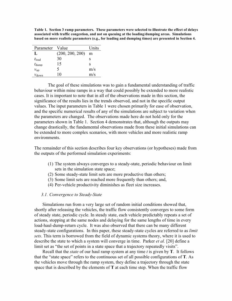
Table 1. Section 3 ramp parameters. These parameters were selected to illustrate the effect of delays associated with traffic congestion, and not on queuing at the loading/dumping areas. Simulations based on more realistic parameters (e.g., for loading and dumping times) are presented in Section 4.

Parameter Value Units L (200, 200, 200) m tload 30 s tdump 15 s vup 5 m/s vdown 10 m/s

The goal of these simulations was to gain a fundamental understanding of traffic behaviour within mine ramps in a way that could possibly be extended to more realistic cases. It is important to note that in all of the observations made in this section, the significance of the results lies in the trends observed, and not in the specific output values. The input parameters in Table 1 were chosen primarily for ease of observation, and the specific numerical results of any of the simulations are subject to variation when the parameters are changed. The observations made here do not hold only for the parameters shown in Table 1. Section 4 demonstrates that, although the outputs may change drastically, the fundamental observations made from these initial simulations can be extended to more complex scenarios, with more vehicles and more realistic ramp environments. The remainder of this section describes four key observations (or hypotheses) made from the outputs of the performed simulation experiments:

(1) The system always converges to a steady-state, periodic behaviour on limit sets in the simulation state space;

(2) Some steady-state limit sets are more productive than others; (3) Some limit sets are reached more frequently than others; and, (4) Per-vehicle productivity diminishes as fleet size increases.

3.1. Convergence to Steady-State

Simulations run from a very large set of random initial conditions showed that, shortly after releasing the vehicles, the traffic flow consistently converges to some form of steady state, periodic cycle. In steady state, each vehicle predictably repeats a set of actions, stopping at the same nodes and delaying for the same lengths of time in every load-haul-dump-return cycle. It was also observed that there can be many different steady-state configurations. In this paper, these steady-state cycles are referred to as limit sets. This term is borrowed from the field of dynamic systems theory, where it is used to describe the state to which a system will converge in time. Parker et al. [20] define a limit set as “the set of points in a state space that a trajectory repeatedly visits”.

Recall that the state of our haul ramp system at any time t is given by T. It follows that the “state space” refers to the continuous set of all possible configurations of T. As the vehicles move through the ramp system, they define a trajectory through the state space that is described by the elements of T at each time step. When the traffic flow

converges to a periodic cycle (i.e., a limit set), this trajectory forms a loop. The set of points (snapshots of T) that make up the loop are what define that particular limit set.

To be completely correct, the definition of the state of a system must also account for the current queuing conditions at the loading and dumping points, because the state of any queues in the ramp cannot be determined by the values in T. It is conceivable that, in some cases, the limit set that a system converges to (after initialization with a given T) could change depending on the queuing conditions at the time of the initialization. This difference would only be of significance in simulations that are initialized with vehicles in the processes of loading, dumping, or queuing, and would not change our fundamental observation.

It is implied by the definition of a limit set that the steady state configuration is determined by the system’s initial condition. In this way, each limit set can be thought of as having a convergence field within the state space, and any initialization state that falls within that field will eventually converge to that limit set. By definition, the convergence fields of any two limit sets in a given system must be mutually exclusive. If the assumption is made that all possible states of initialization will eventually converge to steady state behaviour, then the state space can also be completely defined as the set of convergence fields of all the possible limit sets.

With two and three vehicles, the collective behaviour of the vehicles can be observed by plotting the positions of the vehicles against one another over time in Cartesian coordinates. This type of plot is shown for the two-vehicle case in Figure 4. The loops in Figure 4 are generated by mapping the first row of T (which contains the vehicle position vector, (p1, p2)) over time while the system operates in steady state. Each distinct loop represents a different steady state configuration.

0 0.5 1 1.5 2 2.5 30

0.5

1

1.5

2

2.5

3

p1

p 2

"A"

"B"

Figure 4. A visualization of the limit sets in the two-vehicle case.

In Figure 4, the overall symmetry of the plot about the line p1 = p2 is explained by the reassignment of vehicle numbers within the same type of limit set. Because the vehicles are identical, reassigning the vehicle numbers has no practical consequence other than complicating the task of identifying unique limit sets. The loops labelled as “B” in Figure 4 actually represent the same vehicle behaviours, but with the opposite assignment of numbers. The loop labelled as “A” can also have a mirrored configuration, but it is not visible on the plot because the loop itself is symmetrical about the line of reflection.

With just two vehicles, a given limit set can have two possible vehicle numbering configurations. In the general case with n vehicles, the vehicle numbers can be assigned in n! different ways. These reconfigurations are in fact distinct limit sets, but in this paper they are grouped as one. This assumption is made for simplicity, because the collective vehicle behaviours and productivities achieved are the same.

When a ramp system has converged to a steady state, plotting the positions of the vehicles over time allows for a clear visualization of the individual vehicle behaviours characteristic of the limit set that the system is operating in. This is shown for the two-vehicle case in Figure 5. The upper plot shows the two-vehicle system operating in limit set “A”, and the lower plot shows the same system operating in limit set “B”.

0 100 200 300 400 500 600 700 800 900 10000

0.5

1

1.5

2

2.5

3Limit Set A

Time (s)

Posi

tion

0 100 200 300 400 500 600 700 800 900 10000

0.5

1

1.5

2

2.5

3Limit Set B

Time (s)

Posi

tion

Figure 5. Vehicle motions plotted over time (two-vehicle case).

3.2. Some Limit Sets are More Productive than Others

Let productivity be determined by the average time taken for a vehicle to complete a single load-haul-dump-return cycle while operating in steady state (shorter cycle times indicate greater productivity). Simulations were repeatedly run from random initializations of T. By exhaustive simulation in this way, nearly all of the possible limit sets for the system (in both the two- and three-vehicle cases) could be observed. It was discovered that, in the same ramp with the same number of vehicles, some of the limit sets were more productive than others.

In these tests, all of the vehicles were observed to complete just one load-haul-dump-return cycle in each iteration of a limit set period (in other words, the vehicle cycle times equalled the limit set periods). The discussion in Section 4 will show that this is not always the case, necessitating a clear distinction between the measurements of limit set period lengths and average vehicle cycle times when discussing ramp productivity. With two vehicles operating in the short ramp, the vehicle cycle times in the most productive limit set (“B”) were found to be 4.0 % shorter than those in the least productive limit set (“A”). In the three-vehicle case, the difference was 7.4 %. In mining, due to scale and timeframe of operations, even small improvements, such as this, can result in significant revenue.

3.3. Some Limit Sets are Reached More Frequently than Others

One convenient method of cataloguing limit sets is by their periods. Using the same repeated random initialization technique described in Section 3.2, the periods of all of the possible limit sets in the basic two- and three-vehicle cases were recorded. After many simulations were randomly initialized and run to convergence, observations could be made regarding the relative likelihoods of convergence to limit sets with different periods. Using this technique, it was found that some limit set periods occurred significantly more frequently than others. The results from the basic two- and three-vehicle simulations are presented as histograms in Figure 6.

240 245 250 255 260 265 270 275 280 285 2900

100

200

300

400

500

600

Limit Set Period (seconds)

Num

ber o

f Occ

urre

nces

Two−Vehicle Limit Sets

240 245 250 255 260 265 270 275 280 285 2900

100

200

300

400

500

600

Limit Set Period (seconds)

Num

ber o

f Occ

urre

nces

Three−Vehicle Limit Sets

Figure 6. Histograms showing the limit set periods and their relative frequencies of occurrence for the two- and three-vehicle cases.

If the assumption is made that each bar in the histograms corresponds to one unique limit set (and all of its equivalent labelling permutations), then the result demonstrating the varying likelihoods of convergence implies that the convergence fields of the of the different limit sets are of non-uniform size. With random initializations, the frequency of convergence to a particular limit set must be directly proportional to the size of its convergence field. Unfortunately, the results in Section 4 demonstrate that it is possible (and common) for otherwise unique limit sets to have the same period lengths, which complicates the analysis. In any case, it is still a significant result to note that

certain limit set periods (and vehicle cycle times) appear to occur more frequently than others.

3.4. Productivity per Vehicle Diminishes as Fleet Size Increases

With all other factors left unchanged, the three-vehicle simulations produced limit sets with longer average cycle times than the two-vehicle simulations. Because of the increased delays due to traffic congestion in the three-vehicle case, the individual vehicles were required to stop and wait more frequently, and/or for longer periods of time. As expected, the overall productivity of the ramp (the total haulage rate) was seen to increase with the addition of extra vehicles, but the average productivity per vehicle decreased.

For comparison, the simulation was also run with just one vehicle on the ramp in order to create a benchmark by removing all delays associated with traffic congestion. In that case, the lone vehicle was able to travel up and down the ramp without stopping at any of the passing bays, and it was able to achieve a cycle time of 225 s. This cycle time can be viewed as a benchmark against which the per-vehicle productivities of the two- and three-vehicle cases can be measured (in the same ramp environment). With two vehicles, the average cycle time increased to 244.8 s, which indicated a decrease in per-vehicle productivity of 8.8 %. With a third vehicle added, the average per-vehicle productivity decreased by 22.1 % from the one-vehicle case.

4. Advanced Ramp Scenario

The set of simulations described in this section were run for a larger ramp environment made up of seven 250-m long ramp segments, and the number of vehicles deployed in the ramp was varied from one to nine. The input parameters for the simulations described in this section are shown in Table 2.

Table 2. Section 4 ramp parameters. Although these parameters were selected to approximate reality (based on discussions with mine operators), the objective of the simulations was to draw general conclusions about traffic patterns rather than to model a specific scenario. Relatively small changes to the vehicle speeds (e.g., due to type of machine or ramp grade) do not change the resulting fundamental observations about the existence of limit cycles in ramp traffic.

Parameter Value Units L (250, 250, 250, 250, 250, 250, 250) m tload 90 s tdump 30 s vup 5 m/s vdown 10 m/s

The primary goal of these simulations was to determine if the basic observations

made in Section 3 could be extended to cases involving a larger ramp and more vehicles,

which would be more typical of a real mining operation. This paper presents the results for simulations involving up to five vehicles5.

4.1. One-Vehicle Baseline

With no traffic congestion from other vehicles, a lone vehicle can complete one full cycle in 645 s for the ramp parameterized by Table 2. This represents the minimum possible per-vehicle cycle time, which serves as a baseline for what follows.

4.2. Two and Three Vehicles

Figure 7 shows the possible limit sets for the two-vehicle case. After accounting for symmetry, there are three possible limit sets. Interestingly, despite displaying very distinct behaviours, they all have exactly the same period of 660 s, which demonstrates that analysis of the histogram plots alone (e.g., Figure 6) is not sufficient.

0 200 400 600 800 1000 1200 1400 1600 1800 20000

2

4

6

Posi

tion

Time (s)

Limit Set 1

0 200 400 600 800 1000 1200 1400 1600 1800 20000

2

4

6

Posi

tion

Time (s)

Limit Set 2

0 200 400 600 800 1000 1200 1400 1600 1800 20000

2

4

6

Time (s)

Posi

tion

Limit Set 3

Figure 7. Comparison of the three limit set types exhibited in the two-vehicle case. All three have identical period lengths (660 s).

5 Simulations were run up to nine vehicles. But, for brevity’s sake, the most important findings can be explained with only five vehicles.}.

The three-vehicle case is more interesting. The histogram, shown in Figure 8, exhibits three limit set period lengths that range from 1365 s to 1367 s. As in the two-vehicle case, each bar represents more than one distinct limit set. For example, both limit sets plotted in Figure 9 have periods equal to 1365 s.

1365 1365.2 1365.4 1365.6 1365.8 1366 1366.2 1366.4 1366.6 1366.8 13670

50

100

150

200

250

Period (s)

Freq

uenc

y

Figure 8. Limit set periods for the three-vehicle case.

0 200 400 600 800 1000 1200 1400 1600 1800 20000

1

2

3

4

5

6

7

Time (s)

Posi

tion

Limit Set 1

0 200 400 600 800 1000 1200 1400 1600 1800 20000

1

2

3

4

5

6

7

Time (s)

Posi

tion

Limit Set 2

Figure 9. Sample limit sets from the three-vehicle case (both with 1365 second periods).

What is more, in the three-vehicle case every limit set contains more than one haulage cycle per period. This explains large increase in period length when compared with the two-vehicle case. Thus, it is important to distinguish between the cycle times and the limit set periods. In this case, there are always two haulage cycles per period. Thus, for the limit set with period 1365.8 s, the average haulage time is 682.9 s, which represents an increase of nearly 23 s over the two-vehicle case due to increased congestion.

4.3. Four and Five Vehicles

Comparison of the four- and five-vehicle cases represents the main result of this section. With four vehicles in the same eight-node ramp, all of the limit sets included only one cycle per period. Repeated simulations revealed only two possible limit set periods and an average period length of 735.1 s, which is an increase of 52.2 s over the three-vehicle case. Once again, it is worth noting that although there were only two different possible limit set periods identified, the system was shown to regularly converge to more than two types of limit sets.

With a fifth vehicle added, the simulator produced some very interesting and unexpected results. Approximately 75 % of the randomly generated initial states were observed to converge to limit sets with surprising period lengths of 33,455 s (which allowed every vehicle to complete 46 cycles per period). 20 % of the simulations yielded results more like those observed in the other tests, having periods of 1425 s with two

cycles in each period. More infrequently, the system converged to limit sets with periods that had even greater lengths of 243,300 s, with 322 cycles per period.

Most interestingly, it was found that with five vehicles, a significant majority of the initial states converged to behaviours that yielded average cycle times of just over 727 s. These included all of the cases reported to have converged to limit sets with periods of 33,455 s and 243,300, along with the few non-convergence cases. The cases with shorter limit set periods (1425 s) had notably shorter cycle times of just 712.5 s.

Oddly, these vehicle cycle times were shorter than any of the cycle times achieved in the four-vehicle simulations. The most productive limits set in the five-vehicle case achieved a 3.1 % improvement in per-vehicle production over the most productive four-vehicle configurations. This is counterintuitive result since one would expect that adding vehicles to the system should result in increased congestion and, thus, decreased productivity.

These results make a strong case for the potential of multi-vehicle coordination in mine haulage ramps. At the very least, this anomaly serves as an indication that the basic lockout system is certainly a sub-optimal policy. Ideally, the four-vehicle case should be able to at least duplicate (and likely improve upon) the results achieved in the five-vehicle case. This can be easily demonstrated by considering the addition of a “phantom vehicle” to the same four-vehicle simulation, which would perturb the behaviour and allow the system to achieve the improved cycle times reached in the five-vehicle case.

Figure 10 compares the fastest limit sets in the two scenarios. Qualitatively, one can see that the five-vehicle scenario kept the vehicles fairly evenly spread throughout the ramp, effectively avoiding delays due to queuing. The opposite was true in the four-vehicle case, where some of the vehicles trailed each other closely, resulting in alternating periods of high congestion followed by long intervals devoid of any queuing at the loading and dumping points. A more optimal policy would clearly stabilize and distribute the arrivals of vehicles at the loading and dumping points in order to minimize queuing delays.

0 200 400 600 800 1000 1200 1400 1600 1800 20000

2

4

6

Four vehicles, 735 second cycles

Posi

tion

Time (s)

0 200 400 600 800 1000 1200 1400 1600 1800 20000

2

4

6

Five vehicles, 712.5 second cycles, 1425 second period

Posi

tion

Time (s)

Figure 10. A comparison of the most productive limit sets in the four and five vehicle cases.

5. Conclusions

(1) The research discussed in this paper demonstrates that, at a fundamental level, periodic patterns underlie the behaviours of vehicles that operate in environments designed to resemble underground mine ramps. Understanding these patterns is important because the overall productivity of a simulated ramp depends on the type of steady-state configuration (limit set) to which the system converges.

(2) The simulation results discussed in this paper show that the concepts of limit sets and convergence to steady state traffic flow can be extended beyond the basic cases to include larger ramps with more vehicles.

(3) It was demonstrated that different limit sets could achieve different productivities, even with the same number of vehicles operating in the same ramp layout. It was observed that some of the limit sets resulted in “bunching” of the vehicles together, sometimes causing queuing at the loading or dumping points, while others did a better job of distributing the vehicles throughout the ramp. In practice, there would be advantages to preventing this kind of congestion.

(4) It seems intuitive that the productivity achieved by each vehicle in a ramp should decrease gradually as more and more vehicles are added, as a result of the increasing traffic congestion. In general, this was shown to be the case, but the simulations revealed two surprising exceptions that could be exploited.

(5) The results from the tests described in this paper provide a strong case for the potential of improving upon the non-optimal basic lockout policy, albeit within an idealized ramp environment. The notion of asymptotically stable limit sets may be affected by the inclusion of stochastic variables and other random perturbations, but the existence of fundamental behaviours clearly provides significant insight about the problem of ramp production optimization.

Acknowledgements

Thanks to Ivan Zelina and Dennis Kattowitz (Micromine Pty Ltd., Western Australia) and Jon Peck (Peck Tech Consulting Ltd., Montréal, Canada) for fruitful discussions about the problems and realities of underground ramp management. This work was supported in part by the Natural Sciences and Engineering Research Council of Canada (NSERC) under grant 371452-2009.

References

[1] Elevli B, Demirci A, Dayi O. Underground haulage selection: Shaft or ramp for a small-scale underground mine. J South African Inst Min Metall 2002;102:255–60.

[2] McCarthy PL, Livingstone R. Shaft or decline? An economic comparison. AIG Bull 1993;14:45–56.

[3] Atlas Copco Rock Drills AB. Underground Mining Methods. 1st ed. Ulf Linder; 2003.

[4] Sturgul JR, Jacobsen WL, Tecsa TL. Modeling two-way traffic in an underground one-way decline. Proc. 5th Int. Symp. Mine Plan. Equip. Sel., Sao Paulo, Brazil: A. A. Balkema; 1996, p. 87–90.

[5] Vagenas N. Dispatch control of a fleet of remote-controlled automatic load-haul-dump vehicles in underground mines. Int J Prod Res 1991;29:2347–63.

[6] Beaulieu M, Gamache M. An enumeration algorithm or solving the fleet management problem in underground mines. Comput Oper Res 2006:1606–24.

[7] Gamache M, Cohen P, Grimard R, Bigras L-P. Fleet management system for underground mines. CIM Bull 2004;97:66–70.

[8] Gamache M, Grimard R, Cohen P. A shortest-path algorithm for solving the fleet management problem in underground mines. Eur J Oper Res 2005;166:497–506.

[9] Bigras L-P, Gamache M. Considering displacement modes in the fleet management problem. Int J Prod Res 2005;43:1171–84.

[10] Frank O. Two-way traffic on a single line of railway. Oper Res 1966;14:801–11.

[11] Kray D, Harker PT, Chen B. Optimal pacing of trains in freight railroads: Model formulation and solution. Oper Res 1991;39:82–9.

[12] Peasgood M, Clark CM, McPhee J. A complete and scalable strategy for coordinating multiple robots within roadmaps. IEEE Trans Robot 2008;24:283–92.

[13] Smith SL, Tumová J, Belta C, Rus D. Optimal path planning under temporal logic constraints. Proc. IEEE/RSJ Int. Conf. Intell. Robot. Syst., Taipae, Taiwan: 2010, p. 3288–93.

[14] Smith SL, Tumová J, Belta C, Rus D. Optimal path planning for surveillance with temporal-logic constraints. Int J Rob Res 2011;30:1695–708.

[15] Sturgul JR. Mine Design: Examples Using Simulation. Society for Mining, Metallurgy, and Exploration (SME); 2000.

[16] Vagenas N. Applications of discrete-event simulation in Canadian mining operations in the nineties. Int J Surf Mining, Reclam Environ 1999;13:77–8.

[17] Liu J, Liu X, Koo TJ, Sinopoli B, Sastry S, Lee EA. A hierarchical hybrid system model and its simulation. Proc. 38th IEEE Conf. Decis. Control, Phoenix, AZ: 1999, p. 3508–13.

[18] Artan U, Marshall JA, Lavigne NJ. Robotic mapping of underground mine passageways. Trans IMM (Part A) Min Technol 2011;120:18–24.

[19] Lavigne NJ, Marshall JA. A landmark-bounded method for large-scale underground mine mapping. J F Robot 2012;29:861–79.

[20] Parker TS, Chua LO. Practical Numerical Algorithms for Chaotic Systems. New York: Springer; 1989.