functions of several variables, limits and...

Functions of Several Variables, Limits and Derivatives

Introduction and Goals:

The main goal of this lab is to help you visualize surfaces in three dimensions. We investigate how one can use Maple to evaluate limits of surfaces. We will also look at the Maple syntax for taking partial derivatives of first and higher order. Finally, we will use these derivatives to create a visual image of the relationship between partial derivatives and the slope of the tangent line to the curve formed by the intersection of the surface and a vertical plane. Before You Start:

Make sure that you read and understand the mathematics from the corresponding sections in your textbook. Textbook Correspondence: Stewart 5th Edition: 15.1-15.3. Stewart 5th Edition Early Transcendentals: 14.1-14.3. Thomas’ Calculus 10th Edition Early Transcendentals: 11.1-11.3. Maple Commands and Packages Used: Packages: plots. Commands: plot3d, implicitplot3d. limit, contourplot, spacecurve, seq, diff, D, solve, display. History & Biographies: Maple Commands:

Most of the commands in this lab are stored in the plots package; load it into your worksheet.

> with(plots): Warning, the name changecoords has been redefined

Plotting functions of two variables is done with the plot3d command, if the functions are explicitly defined, and with the implicitplot3d command, if the surface is defined

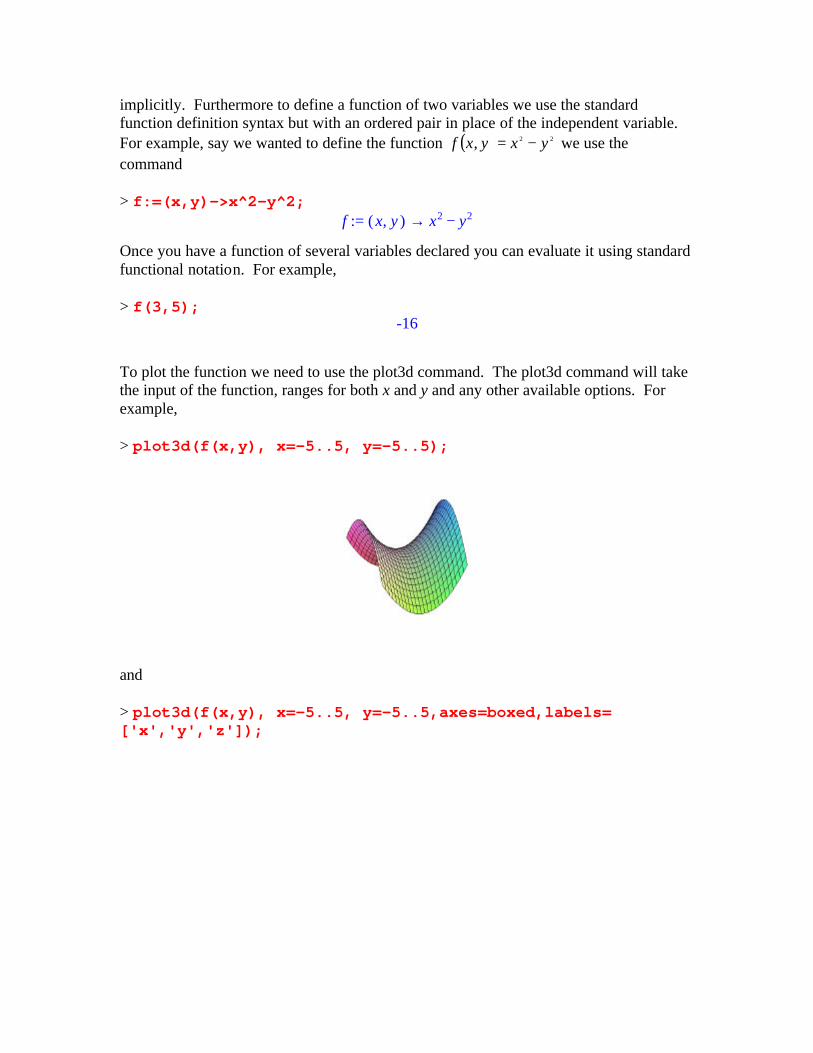
implicitly. Furthermore to define a function of two variables we use the standard function definition syntax but with an ordered pair in place of the independent variable. For example, say we wanted to define the function ( ) 22, yxyxf −= we use the command > f:=(x,y)->x^2-y^2;

:= f → ( ),x y − x2 y2

Once you have a function of several variables declared you can evaluate it using standard functional notation. For example, > f(3,5);

-16

To plot the function we need to use the plot3d command. The plot3d command will take the input of the function, ranges for both x and y and any other available options. For example, > plot3d(f(x,y), x=-5..5, y=-5..5);

and > plot3d(f(x,y), x=-5..5, y=-5..5,axes=boxed,labels= ['x','y','z']);

Surfaces that are implicitly defined, such as 122 −=+− zyxz , need the implicitplot3d command that takes the expression for the surface, ranges for x, y and z and any other available options. For example, > h:=z^2-x^2+z*y=-1;

:= h = − + z2 x2 z y -1

> implicitplot3d(h,x=-3..3,y=-3..3,z=-3..3);

Contour plots are done with the contourplot command. > contourplot(f(x,y),x=-5..5,y=-5..5);

You can superimposed the contour on to the surface using the patchcontour style in the plot3d command. > plot3d(f(x,y), x=-5..5, y=-5..5,axes=boxed,labels= ['x','y','z'],style=PATCHCONTOUR);

Moving the orientation so that you’re looking straight down the z-axis we see the contour clearly on the surface.

Although we cannot create a contour plot of an implicitly defined surface we can use the patchcontour style in the implicitplot3d command to get a rough idea of the contour of the surface. For example, > implicitplot3d(h,x=-3..3,y=-3..3,z=-3..3, style=PATCHCONTOUR);

Limits of functions of two or more variables, as you from your reading, are substantially different from the limits of functions of a single variable primarily because you are no longer coming into the limit point from just two directions but are coming into the limit point from an infinite number of directions. Due to this fact, Maple has a difficult time finding the limits of functions of more than one variable. All we can use Maple for is to get an idea if the limit actually exists or if it does not. If we feel that the limit does not exist we may be able to use Maple to find two different paths into the limit point that do not agree and hence prove that the limit does not exist. We will first consider the

function ( ) 22, yxyxf −= . When looking at limits of functions of several variables in Maple we take two approaches, using the definition to get a graphical verification that the limit exists and using different pathways into the limit point to show that the limit does not exist. First by definition, we see whether or not the function is approaching a single value as we decrease the neighborhood around the limit point. That is we look at smaller and smaller regions around the limit point to see whether or not the surface “flattens out” and becomes well behaved or if becomes not well behaved and has kinks or separations in it. Since this function is continuous everywhere we know that it will have a limit as we approach any point, in particular ( )2,1 . Maple’s limit command will take the limit of a function of two or more variables. Unfortunately, due to the complexity of finding limits of multivariable functions, this command does not always produce the results we want. The limit command takes the function and a point and returns the limit if it can. The limit command may also return undefined if it notices that the limit depends on the pathway chosen to the limit point. For example, > limit(f(x,y),{x=1,y=2});

-3

which is correct. Since, as we will see, the limit command does not always return a value we will also use a graphical approach to this limit. We will begin by graphing the surface close to ( )2,1 and continually decrease the neighborhoods. Notice that as the neighborhood decreases the surface begins to look like a smooth plane, this gives us the intuition that the function does have a limit as we approach the point ( )2,1 . > eps:=0.1;

:= eps 0.1

> plot3d(f(x,y), x=1-eps..1+eps, y=2-eps..2+eps,axes=boxed, labels=['x','y','z']);

> eps:=0.00001;

:= eps 0.00001

> plot3d(f(x,y), x=1-eps..1+eps, y=2-eps..2+eps,axes=boxed, labels=['x','y','z']);

Furthermore, it appears that the limit is –3. Now consider the function ( ) 22

22

,yx

yx

yxg+

+= .

When we graph this surface close to the origin we see that there appears to be four plateaus at two different heights. This alone gives us the intuition that the limit as we approach the origin of this function does not exist. Using the limit command we get the undefined output, which signifies that Maple noticed that the limit depended on the path taken to the origin. > limit(g(x,y),{x=0,y=0});

undefined

Even though Maple said that the limit did not exist, we should still view the surface on smaller and smaller neighborhoods close to the origin to get a better idea of what this function does locally, at the origin. Since the images close to the origin are the same we would believe that this function does not have a limit as we approach the origin. > g:=(x,y)->abs(x^2-y^2)/(x^2-y^2);

:= g → ( ),x y − x2 y2

− x2 y2

> eps:=0.1; := eps 0.1

> plot3d(g(x,y), x=-eps..eps, y=-eps..eps,axes=boxed,labels= ['x','y','z']);

> eps:=0.00001;

:= eps 0.00001

> plot3d(g(x,y), x=-eps..eps, y=-eps..eps,axes=boxed,labels= ['x','y','z']);

Now consider the function ( ) ( )

22

2

,yx

yxyxj+

+= .

> limit(j(x,y),{x=0,y=0});

limit ,

( ) + x y 2

+ x2 y2 { }, = x 0 = y 0

Notice that Maple returned what we gave it, hence Maple could not find the limit nor could it verify that the limit does not exist. We will verify that this limit in fact does not exist. When we graph this surface on a large region we see that at the origin the surface seems to be pinched, giving us the intuition that the limit will not exist as we approach the origin. Zooming in several times we see that the surface close to the origin is still pinched and is not smooth.

> j:=(x,y)->(x+y)^2/(x^2+y^2);

:= j → ( ),x y( ) + x y 2

+ x2 y2

> plot3d(j(x,y), x=-5..5, y=-5..5,axes=boxed,labels= ['x','y','z']);

> eps:=0.1;

:= eps 0.1

> plot3d(j(x,y), x=-eps..eps, y=-eps..eps,axes=boxed,labels= ['x','y','z']);

> eps:=0.000001;

:= eps 0.1 10-5

> plot3d(j(x,y), x=-eps..eps, y=-eps..eps,axes=boxed,labels= ['x','y','z']);

Recall from you reading that to prove that a limit does not exist we simply need to find two pathways into the limit that produced difference numeric values. Here is where Maple comes in handy. Consider this last function ( ) ( )

22

2

,yx

yxyxj+

+= . Notice that there are

two ridges, really a ridge and a valley. If we come into the origin across the top of the ridge we would most likely get a limit of 2. On the other hand, if we come into the origin along the valley we should obtain a limit of 0. All that remains is to figure out the equations of the lines that go across the ridge and the valley. From a bird’s eye view it seems apparent that the line going across the ridge is the line

xy = and the equation of the line going through the valley is xy −=

Substituting xy = and xy −= in for y in the function and taking the limit as x goes to 0 gives us two different limit values. Hence the limit does not exist for this function as we approach the origin.

> limit(j(x,x),x=0); 2

> limit(j(x,-x),x=0); 0

Similarly we could come in on the line 0=y , in other words come along the x-axis. The limit here is 1, giving us yet a third value. > limit(j(x,0),x=0);

1

If we take the function ( ) 22

22

,yx

yx

yxg+

+= that had the four plateaus we see that if we come in

on either the x-axis or the y-axis we should get two different values, most likely 1 and –1. This shows us that the limit does not exist. > limit(g(x,0),x=0);

1

> limit(g(0,y),y=0); -1

Now let’s consider a function that has a singularly at the origin, for example

( ) 221,

yxyxk

+= . Maple’s limit function produces,

> limit(k(x,y),{x=0,y=0});

undefined

Notice if we graph this surface relatively close to the origin there seems to be the spike. Zooming in even further shows that spike is still there, giving us the feeling that the limit does not exist at the origin. > k:=(x,y)->1/(x^2+y^2);

:= k → ( ),x y1

+ x2 y2

> eps:=0.1; := eps 0.1

> plot3d(k(x,y), x=-eps..eps, y=-eps..eps,axes=boxed,labels= ['x','y','z']);

> eps:=0.001;

:= eps 0.001

> plot3d(k(x,y), x=-eps..eps, y=-eps..eps,axes=boxed,labels= ['x','y','z']);

Taking the limit to the origin along the x-axis, we see again that the limit certainly does not exist, not because we go to different values on two different pathways but because the limit on one particular path is non-numeric. > k:=(x,y)->1/(x^2+y^2);

:= k → ( ),x y1

+ x2 y2

> limit(k(x,0),x=0); ∞

As with any computer program one must always take graphic images a grain of salt. Consider the function ( )

1122

22

,−++

+=yx

yxyxh . As above, Maple’s limit command does not

produce an adequate answer. > limit(h(x,y),{x=0,y=0});

limit , + x2 y2

− + + x2 y2 1 1{ }, = x 0 = y 0

By rationalizing the denominator we see that this function does have a limit as we approach the origin, unfortunately looking at this graphical we might come to a different conclusion. As we get closer and closer to the origin part of the graph seems to become very planar but the other part of the graph is extremely jagged. At the origin the function does not exist and hence we get a hole in the graph. Zooming in further we find that part of the graph is still jagged in the other simply disappeared. So although the limit of this function as we approach the origin does exist, our graphical analysis would lead us to believe otherwise. > h:=(x,y)->(x^2+y^2)/(sqrt(x^2+y^2+1)-1);

:= h → ( ),x y + x2 y2

− + + x2 y2 1 1

> eps:=0.1;

:= eps 0.1

> plot3d(h(x,y), x=-eps..eps, y=-eps..eps,axes=boxed,labels= ['x','y','z']);

> eps:=0.01;

:= eps 0.01


> eps:=0.0001;

:= eps 0.0001


> eps:=0.0000001;

:= eps 0.1 10-6


Finding partial derivatives in Maple is as simple as finding derivatives of single variable functions that you did back in Calculus I, we simply use the diff command. The diff command takes two parameters, the first is the function and the second is the variable that we are differentiating with respect to. For example, > diff(j(x,y),x);

− 2 ( ) + x y

+ x2 y2

2 ( ) + x y 2 x

( ) + x2 y22

> diff(j(x,y),y);

− 2 ( ) + x y

+ x2 y2

2 ( ) + x y 2 y

( ) + x2 y22

We can also do higher order derivatives simply by adding variables to the end of the argument list in the diff command. For example, the second partial derivative with respect to x of this function is > diff(j(x,y),x,x);

− + − 2

+ x2 y2

8 ( ) + x y x

( ) + x2 y22

8 ( ) + x y 2 x2

( ) + x2 y23

2 ( ) + x y 2

( ) + x2 y22

The third partial derivative with respect to x is

> diff(j(x,y),x,x,x);

− + − − + 12 x

( ) + x2 y22

48 ( ) + x y x2

( ) + x2 y23

12 ( ) + x y

( ) + x2 y22

48 ( ) + x y 2 x3

( ) + x2 y24

24 ( ) + x y 2 x

( ) + x2 y23

We can also find mixed partial derivatives. > diff(j(x,y),x,y);

− − + 2

+ x2 y2

4 ( ) + x y y

( ) + x2 y22

4 ( ) + x y x

( ) + x2 y22

8 ( ) + x y 2 x y

( ) + x2 y23

> diff(j(x,y),y,x);

− − + 2

+ x2 y2

4 ( ) + x y y

( ) + x2 y22

4 ( ) + x y x

( ) + x2 y22

8 ( ) + x y 2 x y

( ) + x2 y23

> diff(j(x,y),x,y)-diff(j(x,y),y,x); 0

> diff(j(x,y),x,y,y,x); 64 y x

( ) + x2 y23

16 y2

( ) + x2 y23

192 ( ) + x y y2 x

( ) + x2 y24

8

( ) + x2 y22

32 ( ) + x y x

( ) + x2 y23

16 x2

( ) + x2 y23 + − − + +

192 ( ) + x y x2 y

( ) + x2 y24

32 ( ) + x y y

( ) + x2 y23

384 ( ) + x y 2 x2 y2

( ) + x2 y25

48 ( ) + x y 2 y2

( ) + x2 y24 − + + −

48 ( ) + x y 2 x2

( ) + x2 y24

8 ( ) + x y 2

( ) + x2 y23 − +

We can also use the $ command to do higher order derivatives with respect to the same variable. For example, the third and 7th derivatives with respect to x are, > diff(j(x,y),x$3);

− + − − + 12 x

( ) + x2 y22

48 ( ) + x y x2

( ) + x2 y23

12 ( ) + x y

( ) + x2 y22

48 ( ) + x y 2 x3

( ) + x2 y24

24 ( ) + x y 2 x

( ) + x2 y23

> diff(j(x,y),x$7); 403200 ( ) + x y 2 x3

( ) + x2 y26

40320 ( ) + x y 2 x

( ) + x2 y25

241920 ( ) + x y x2

( ) + x2 y25

967680 ( ) + x y 2 x5

( ) + x2 y27− + + +

806400 ( ) + x y x4

( ) + x2 y26

645120 ( ) + x y 2 x7

( ) + x2 y28

10080 ( ) + x y

( ) + x2 y24

645120 ( ) + x y x6

( ) + x2 y27 − − − +

30240 x

( ) + x2 y24

161280 x3

( ) + x2 y25

161280 x5

( ) + x2 y26 − + −

One problem with the diff command is that the result is an expression and not a function. We can turn it into a function by using the unapply command on the result of the diff command. This way we can set the partial derivatives to function names so that we can use their values in other expressions. For example, > fx:=unapply(diff(f(x,y),x),x,y);

:= fx → ( ),x y 2 x

> fx(5,3); 10

> fy:=unapply(diff(f(x,y),y),x,y); := fy → ( ),x y −2 y

> fy(5,3); -6

Another command that can be used for the partial derivative is the D command. This command differs slightly in syntax and output from the diff command. First of all, the partial derivative with respect to the first variable is denoted by [1] and the partial derivative with respect to the second variable is denoted by [2]. Another difference is that the function we are differentiating is input by using only the function name and not the functional notation. The output of the D command is actually a function and can be evaluated directly or assigned to a name. For example, > fx:=D[1](f);

:= fx → ( ),x y 2 x

> fx(5,3); 10

> fy:=D[2](f); := fy → ( ),x y −2 y

> fy(5,3); -6

> D[1](f)(5,3); 10

> D[2](f)(5,3); -6

We can also take higher order partial derivatives simply by using the @@ command. For example, > (D[1]@@3)(j);

→ ( ),x y − + − − + 12 x

( ) + x2 y22

48 ( ) + x y x2

( ) + x2 y23

12 ( ) + x y

( ) + x2 y22

48 ( ) + x y 2 x3

( ) + x2 y24

24 ( ) + x y 2 x

( ) + x2 y23

> jyyy:=(D[2]@@3)(j); jyyy :=

→ ( ),x y − + − − + 12 y

( ) + x2 y22

48 ( ) + x y y2

( ) + x2 y23

12 ( ) + x y

( ) + x2 y22

48 ( ) + x y 2 y3

( ) + x2 y24

24 ( ) + x y 2 y

( ) + x2 y23

> jyyy(5,3); 2415

83521

Maple can also do implicit differentiation in this case your parameter list consists of the expression to be implicitly differentiated and then two variables the first variable is the one being differentiated and the second variable is the one we are differentiating with respect to. Again we can turn the derivative into a function using the unapply command. For example, recall that the surface 122 −=+− zyxz looks like,

The following three commands find the partial of z with respect to x, the partial of z with respect to y, and the partial of y with respect to z. > h:=z^2-x^2+z*y=-1;

:= h = − + z2 x2 z y -1

> implicitdiff(h,z,x);

2 x + 2 z y

> implicitdiff(h,z,y);

−z + 2 z y

> implicitdiff(h,y,z);

− + 2 z yz

There are two points on the surface where x is 5 and y is 4, they can be found through the following command. > solve(subs({x=5,y=4},h));

,− + 2 2 7 − − 2 2 7

To find the partial derivative of z with respect to y of this surface at these two points we first create a function of three variables which represents the partial derivative of z with respect to y then we evaluate the functional values at the two points. > hzy:=unapply(implicitdiff(h,z,y),x,y,z);

:= hzy → ( ), ,x y z −z + 2 z y

> hzy(5,4,-2+2*7^(1/2));

−( )− + 2 2 7 7

28

> hzy(5,4,-2-2*7^(1/2)); ( )− − 2 2 7 7

28

The next series of commands is to help us understand what the partial derivative actually is, at least graphically. Consider the function ( ) ( ) ( )xyyxyxk −−−= 3cos2sin, . We would like to examine what the partial derivative with respect to y at the point ( )1,2 means. > k:=(x,y)->sin(x-2*y)-cos(3*y-x);

:= k → ( ),x y − ( )sin − x 2 y ( )cos − 3 y x

> plot3d(k(x,y), x=0..Pi, y=0..Pi,axes=boxed,labels= ['x','y','z']);

First, since the partial derivative is with respect to y this means that x is being held constant specifically since we’re interested in the point ( )1,2 x is being held constant at 2. So if we put a vertical plane through the surface at 2=x we obtain the following image. > display(plot3d(k(x,y), x=0..Pi, y=0..Pi,axes=boxed,labels= ['x','y','z']),implicitplot3d(x=2,x=0..Pi, y=0..Pi,z=-1..1));

Next we take the partial derivative of our function with respect to y and use the unapply command to assign a name to the derivative. Then we evaluate this function at ( )1,2 giving the following numeric answer. > ky:=unapply(diff(k(x,y),y),x,y);

:= ky → ( ),x y − − 2 ( )cos − x 2 y 3 ( )sin − + 3 y x

> ky(2,1); − + 2 3 ( )sin 1

From your reading you know that this value represents the slope of the tangent line to the curve created from the intersection of the surface and the vertical plane. To graph it we simply use the spacecurve command, fixing x at 2, setting y to t+1 and z to the functional value at ( )1,2 plus the slope of the line times t. Graphing all three of these together gives the following image. > display(plot3d(k(x,y), x=0..Pi, y=0..Pi,axes=boxed,labels= ['x','y','z']),implicitplot3d(x=2,x=0..Pi, y=0..Pi,z=-1..1),spacecurve([2,1+t,ky(2,1)*t+k(2,1)],t=-1..2,color=black,thickness=4));

Finally we can create a command using the seq command along with the display command to create an animation of the tangent line as the y value ranges from 0 to π . > display(seq(display(plot3d(k(x,y), x=0..Pi, y=0..Pi, axes=boxed,labels=['x','y','z']),implicitplot3d(x=2,x=0..Pi, y=0..Pi,z=-1..1),spacecurve([2,Pi*n/20+t,ky(2,Pi*n/20)*t+ k(2,Pi*n/20)],t=-1..1,color=black,thickness=4)),n=0..20), insequence=true);

We will discuss animation bore in later labs but we will at least dissect this command to see how it works. First note that the inside display command is exactly like the command we used above to graph the surface, plane and tangent line, with the exception of

Pi*n/20 used in place of 1. Note that if n is 0 then this value is 0, the starting point for the y range and if the value of n is 20 then this value is π , the ending point for the y range. Thus if we let n range from 0 to 20 we will divide the y range up into 20 equal segments and hence get 21 images all with a slightly different y value. display(plot3d(k(x,y), x=0..Pi, y=0..Pi, axes=boxed,labels=['x','y','z']),implicitplot3d(x=2,x=0..Pi, y=0..Pi,z=-1..1),spacecurve([2,Pi*n/20+t,ky(2,Pi*n/20)*t+ k(2,Pi*n/20)],t=-1..1,color=black,thickness=4)) What creates the 21 images is the seq command seq(display(plot3d(k(x,y), x=0..Pi, y=0..Pi, axes=boxed,labels=['x','y','z']),implicitplot3d(x=2,x=0..Pi, y=0..Pi,z=-1..1),spacecurve([2,Pi*n/20+t,ky(2,Pi*n/20)*t+ k(2,Pi*n/20)],t=-1..1,color=black,thickness=4)),n=0..20) note that the only thing that was done here was to create a sequence of displays as n goes from 0 to 20. Finally, the outside display command with the insequence=true option binds all of the images together into an animation. > display(seq(display(plot3d(k(x,y), x=0..Pi, y=0..Pi, axes=boxed,labels=['x','y','z']),implicitplot3d(x=2,x=0..Pi, y=0..Pi,z=-1..1),spacecurve([2,Pi*n/20+t,ky(2,Pi*n/20)*t+ k(2,Pi*n/20)],t=-1..1,color=black,thickness=4)),n=0..20), insequence=true); Exercises: 1. The following exercises concern the function )sin(),( xyyxf = .

a. Graph this function on the region [ ] [ ]5,55,5 −×− . b. Find the limit of this function as we approach ( )4,3 using the limit command. c. Find the limit of this function as we approach ( )4,3 using graphical analysis. d. What is the limit of this function as we approach ( )4,3 ? What is the justification

for your answer? e. Find the all of the first and second partials of the function. f. Create a display of the surface, vertical plane and tangent line that represents a

visual interpretation of the partial derivative with respect to x at the point ( )4,3 .

g. Create a display of the surface, vertical plane and tangent line that represents a visual interpretation of the partial derivative with respect to y at the point ( )4,3 .

h. If we are standing at the point ( )4,3 which direction, x or y, is increasing at a faster rate.

i. Create an animation like the one in the lab that represents a visual interpretation of the partial derivative with respect to x.

j. Create an animation like the one in the lab that represents a visual interpretation of the partial derivative with respect to y.

2. The following exercises concern the function 22

23

),(yx

yxyxf

+= .


for your answer? Hint: if Maple did not return an acceptable answer and if you graphical analysis suggests a limit you may wish to try the squeeze theorem.

e. Find the all of the first and second partials of the function. f. Create a display of the surface, vertical plane and tangent line that represents a

visual interpretation of the partial derivative with respect to x at the point ( )2,1 . g. Create a display of the surface, vertical plane and tangent line that represents a

visual interpretation of the partial derivative with respect to y at the point ( )2,1 . h. If we are standing at the point ( )2,1 which direction, x or y, is increasing at a

faster rate. i. Create an animation like the one in the lab that represents a visual interpretation

of the partial derivative with respect to x. j. Create an animation like the one in the lab that represents a visual interpretation

of the partial derivative with respect to y.


2

),(yx

yxyxf

+= .


for your answer? e. Find the all of the first and second partials of the function. f. Create a display of the surface, vertical plane and tangent line that represents a



faster rate.

i. Create an animation like the one in the lab that represents a visual interpretation of the partial derivative with respect to x.

j. Create an animation like the one in the lab that represents a visual interpretation of the partial derivative with respect to y.


),(yx

xyyxf

+= .


for your answer? ? Hint: if Maple did not return an acceptable answer and if you graphical analysis suggests a limit you may wish to try the squeeze theorem.

e. Find the all of the first and second partials of the function. f. Create a display of the surface, vertical plane and tangent line that represents a







2),(

22 +−+−

=xyxyxy

yxf .


for your answer? ? e. Find the all of the first and second partials of the function. f. Create a display of the surface, vertical plane and tangent line that represents a






functions of several variables, limits and...

Documents