FUNCTIONAL COEFFICIENT NONSTATIONARY REGRESSION

By

Jiti Gao and Peter C.B. Phillips

September 2013

COWLES FOUNDATION DISCUSSION PAPER NO. 1911

COWLES FOUNDATION FOR RESEARCH IN ECONOMICS YALE UNIVERSITY

Box 208281 New Haven, Connecticut 06520-8281

http://cowles.econ.yale.edu/

Functional Coefficient Nonstationary Regression∗

Jiti Gao† and Peter C. B. Phillips‡

August 3, 2013

Abstract

This paper studies a general class of nonlinear varying coefficient time series mod-

els with possible nonstationarity in both the regressors and the varying coefficient

components. The model accommodates a cointegrating structure and allows for endo-

geneity with contemporaneous correlation among the regressors, the varying coefficient

drivers, and the residuals. This framework allows for a mixture of stationary and non-

stationary data and is well suited to a variety of models that are commonly used in

applied econometric work. Nonparametric and semiparametric estimation methods are

proposed to estimate the varying coefficient functions. The analytical findings reveal

some important differences, including convergence rates, that can arise in the conduct

of semiparametric regression with nonstationary data. The results include some new

asymptotic theory for nonlinear functionals of nonstationary and stationary time se-

ries that are of wider interest and applicability and subsume much earlier research on

such systems. The finite sample properties of the proposed econometric methods are

analyzed in simulations. An empirical illustration examines nonlinear dependencies in

aggregate consumption function behavior in the US over the period 1960 - 2009.

JEL Classifications: C13, C14, C23.

Keywords: Aggregate consumption, Asymptotic theory, cointegration, density, lo-

cal time, nonlinear functional, nonparametric estimation, semiparametric, time series,

varying coefficient model.

∗The authors thank participants at many conferences and seminars for comments on earlier versions of

this work. Gao acknowledges Australian Research Council Discovery Grants Program support under Grant

number: DP1096374. Phillips acknowledges support from the NSF under Grant Nos. SES-0956687 and

SES-1258258.†The University of Adelaide & Monash University.‡Yale University, University of Auckland, University of Southampton, & Singapore Management Univer-

sity.

1

1 Introduction

In recent years, there has been renewed econometric interest in time–varying coefficient

models and their potential applications in economics. These models offer additional flexibil-

ity in practical work and often correspond more closely to underlying theory specifications

than conventional fixed coefficient models. They are usually motivated by the potential in-

stability in economic relations over time, as emphasized in the recent work of Muller and

Petalas (2010). Allowing for time evolution in relationships can be particularly important

when dealing with long time series where the stability of a relationship comes naturally into

question. Examples abound in economics and finance, where institutional and technological

changes may change the effects of fundamentals, the manner in which variables are related,

or possible transitions over time (Phillips and Sul, 2007). Other examples arise in environ-

mental science, resource depletion, and climate change regressions, where trends over long

time frames are evidently endogenous to the sample period selected and considerable flexibil-

ity is needed in the specification of the trend mechanism (see Phillips, 2010). Trending time

series models are also relevant in modeling macroeconomic activity and financial bubbles,

where transition effects can alter cointegrating relations, the form of the nonstationarity,

and introduce shifts in regimes (Phillips and Yu, 2011).

Early work by Robinson (1989) pioneered a nonparametric kernel regression approach to

the estimation of time-varying coefficient models in a deterministic trend framework. Since

then a vast empirical literature has emerged demonstrating that many economic variables

manifest certain types of stochastic trend nonstationarity, primarily of the unit root or near

unit root variety. Such variables include the nominal three month US Treasury bill rate

(e.g., Hamilton 1994; Gao et al 2009a) as well as total consumption and income variables

(e.g., Hall 1978; Campbell and Mankiw 1990; Muellbauer and Lattimore 1999). Some time

series in economics, finance and climatology also show evidence of deterministic drift over

various time periods, including consumer price index series in economics, stock price series in

finance and temperature series in climatology. The nonstationarity in such series may then

involve an unknown deterministic trend function in the systematic component of the model

and there may be further complications arising from the superposition of deterministic and

stochastic trends.

While it may be appealing in principle to address the complications of time varying

coefficient variation and data nonstationarity in a nonparametric regression formulation,

our experience suggests that a completely nonparametric time series approach may not be

workable even for the bivariate case because of poor convergence characteristics arising from

2

multivariate nonstationarity. We are therefore motivated to consider a class of more specific

but still rather general varying coefficient models of the form

Yt = X ′t β(Zt, Ut) + et,

Xt = Xt−1 + µt,

Zt = Zt−1 + νt, (1.1)

where (Ut, µt, νt) is a vector of weakly dependent linear processes generated by a sequence

of independent and identically distributed (iid) variates {ξt}, {et} is a martingale difference

sequence that may be correlated with {ξt}, the functional coefficient β(z, u) is assumed to

be continuous in (z, u) ∈ Rdz+du = (−∞,∞)dz+du , and 1 ≤ t ≤ n with sample size n. Our

specification of (1.1) allows Ut to be multivariate, while Zt is univariate in the case where

the unknown function β(z, u) is estimated by a nonparametric method. The variable Ut may

be endogenously correlated with the innovations (µt, νt), a feature that allows for control

function and augmented regression formulations. A strongly endogenous case of this type

where Ut = (µ′t, ν′t)′ is considered in Example 2.6 below and then in the empirical example

of Section 6. Model (1.1) imposes a unit root structure on Xt and Zt to allow for possible

cointegration in the relationship between Xt and Yt and stochastic trend nonstationarity in

one of the functional coefficient arguments (Zt). As discussed in Remark A.2 of Appendix A,

the discussion of this paper remains valid when Ut is generated by Ut = Λ(ξt−1, · · · , ξt−τ ; ηt),where τ ≥ 1 is a positive integer, Λ(·, · · · , ·) is a measurable function and {ηt} is another

vector of iid random variables and independent of {ξt}. Extensions to near integrated

processes seem also possible under some further conditions and with some modification of

the methods but will not be considered in this paper.

In the parametric case, functional coefficient time series models have already been pro-

posed to deal with various modelling problems involving explanatory variables in the coeffi-

cients of a time series model. For instance, in modelling the dependence between the return

of a share and the market return, a short–term interest rate variable may naturally be in-

volved in determining the betas of a CAPM structure (see, for example, Faff and Brooks

1998), thereby inducing variable dependence in the coefficients. Similar considerations apply

to models of consumption behavior that allow for nonstationarity and varying coefficients

(Hall, 1978). Some research has recently appeared that seeks to address this type of speci-

fication. Following the paper by Cai, Fan and Yao (2000) in the stationary nonparametric

case, Cai, Li and Park (2009) consider a functional coefficient time series model where non-

stationarity is involved in either the parametric regressors or the coefficients, Xiao (2009)

discusses a functional coefficient cointegrating model where nonstationarity is only involved

3

in the parametric regressors, and Sun, Cai and Li (2013) further consider the case where

both the parametric and nonparametric regressors are nonstationary. To cover a wider range

of possible dependencies that may arise in practical work, model (1.1) allows for a varying

coefficient structure in which potentially correlated stationary and nonstationary variables

may both be accommodated within the same model while also permitting endogeneity in

the regressors and covariates that drive the time varying coefficients.

We focus on the leading case where model (1.1) allows for a unit root stochastic trend

in both Xt and Zt. As discussed in Section 2, this model includes many existing nonpara-

metric and semiparametric models. Some useful new models that allow for endogeneity and

incorporate nonstationarity are also covered in this framework. This includes several non-

linear simultaneous equations systems that extend the models used in Newey, Powell and

Vella (1999), Newey and Powell (2003), Su and Ullah (2008), and Florens, Johannes and van

Bellegem (2012) to a nonstationary data setting. In the semiparametric case, (1.1) includes

partially linear models with nonstationary regressors and therefore complements existing

work on semiparametric regression for the stationary regressor case (e.g. Robinson 1988;

Hardle, Liang and Gao 2000; Fan and Yao 2003; Gao 2007; Li and Racine 2007; Terasvirta,

Tjøstheim and Granger 2010).

Other related work for the nonstationary case has covered a variety of more specific

models, including Park and Phillips (1999, 2001) for parameter estimation in parametric

nonlinear regression, Phillips and Park (1998), Karlsen and Tjøstheim (2001) and Karlsen,

Mykelbust and Tjøstheim (2007) for nonparametric nonstationary autoregression, Gao et

al (2009a, 2009b) and Wang and Phillips (2012) for nonparametric specification testing in

a nonstationary environment, Phillips (2009) for nonparametric kernel estimation involv-

ing integrated time series and potentially spurious regression, Wang and Phillips (2009a)

for nonparametric cointegration estimation, Wang and Phillips (2009b) for structural non-

parametric cointegration estimation by kernel resgression, and Gao and Phillips (2010) for

estimation in semiparametric simultaneous systems with time series data.

The present work based on model (1.1) has the following novel features:

(i) The model allows for stochastic trends in both the regressor Xt and the varying coeffi-

cient covariate Zt, while permitting another covariate Ut that is weakly dependent. A

distinctive feature is that (1.1) involves both stationary and nonstationary covariate

drivers in the functional form β(·, ·).

(ii) The system is nonlinear, simultaneous and possibly cointegrating. There is contempo-

raneous correlation among the variates {(Xt, Zt)} and {Ut}, so endogeneity and some

4

heteroskedasticity may be accommodated (the latter by way of martingale difference

sequence innovations and suitable functional limit theory for partial sum processes, as

in Assumption A.1 (iii)-(iv).

(iii) The models and proposed estimation methods provide a natural way of addressing

the endogeneity, cointegration structure, and time varying coefficient behavior that is

inherited from some commonly used modeling frameworks in econometrics and other

disciplines, as discussed in the examples given in Section 2.

(iv) The econometric methods and asymptotic theory involve new results for several non-

parametric and semiparametric regression models in the presence of a mixture of sta-

tionary and integrated regressors. In consequence, both the model (1.1) and the limit

theory considerably extend and complement existing work on asymptotics for nonsta-

tionary and varying coefficient models.

The rest of the paper is organized as follows. Several important examples of model

(1.1) that are suited to econometic implementation are discussed in Section 2. Sections

3 and 4 propose estimation methods and establish asymptotics. The simulations reported

in Section 5 assess the finite sample performance of the proposed estimation methods and

limit theory in three illustrative examples. Section 6 provides an empirical application to

US income, consumption and interest rate data, motivated by theory considerations that

induce a varying coefficient structure (Hall, 1978). The framework of model (1.1) is used

to examine whether more specific existing models, such as those in Campbell and Mankiw

(1990), are empirically supported within this general framework. Section 7 concludes and

discusses future research. Technical assumptions are given in Appendix A together with

some useful preliminary lemmas. Proofs of the main theorems are in Appendix B.

2 Nonparametric and semiparametric cointegration

We discuss several special cases of model (1.1) to illustrate the range of potential application

of our methods and results. Each of these models has its own particular features, which we

consider separately below. Estimation and limit theory for the models along with model

(1.1) are covered in Sections 3 and 4. For convenience, we assume X0 = Z0 = OP (1)

throughout the paper. Extensions that allow for other initializations, including distant

past initializations, may be considered following the lines of Phillips and Magdalinos (2009)

but are not developed here. The dimension of the covariate Zt is dν and when Zt enters

nonparametrically we will assume that dν = 1.

5

Model 2.1 (Multivariate nonparametric model): Let dx = 1 and Xt ≡ 1. Then (1.1) is a

bivariate nonparametric model of the form

Yt = β(Zt, Ut) + et,

Zt = Zt−1 + νt, (2.1)

where both {νt} and {Ut} are linear processes. This system (2.1) allows for the inclusion

of both stationary and nonstationary regressors in the same model. The model may be

interpreted as a nonparametric simultaneous equations model and complements existing

models with only stationary regressors (e.g., Newey, Powell and Vella 1999; Newey and

Powell 2003; Su and Ullah 2008) by permitting nonstationary components.

Model 2.2 (Additive nonparametric regression): Set dx = 2, Xt = (1, 1)′ and β(z, u) =

(β1(z), β2(u))′. In this case, (1.1) is a nonparametric additive model of the form

Yt = β1(Zt) + β2(Ut) + et,

Zt = Zt−1 + νt, (2.2)

where {Ut} is a stationary time series, and both β1(·) and β2(·) are unknown functions.

Model (2.2) includes nonparametric simultaneous equations such as

Yt = m(Zt) + εt,

Zt = Zt−1 + νt,

E [εt|νt, · · · , νt−τ ] = λ(νt, · · · , νt−τ ) (2.3)

for some τ ≥ 0, since system (2.3) can be written in augmented regression (control variate)

form as

Yt = m(Zt) + λ(νt, · · · , νt−τ ) + et,

Zt = Zt−1 + νt, (2.4)

which is a special case of model (2.2) with β1(·) = m(·), β2(·) = λ(·), Ut = (νt, · · · , νt−τ )′

and et = εt − λ(νt, · · · , νt−τ ). We establish an estimation limit theory for model (2.4) in

Corollary 4.2 below.

Model (2.2) complements existing additive models and nonparametric studies (such as

Gao, 2007) where the regressors are all assumed to be stationary. Models (2.1) and (2.2)

have various empirical applications where it is important to allow for nonstationarity, such

as relationships between stock prices, long–term bond yields and the Treasury bill rate.

6

Model 2.3 (Time varying and varying coefficient models): Let Xt = (X1t, 1)′ and β(z, u) =

(β1(z), β2(u))′. In this case, (1.1) is a trending nonparametric model with varying coefficients

of the form

Yt = X ′1tβ2(Ut) + β1(Zt) + et,

X1t = X1t−1 + µt,

Zt = Zt−1 + νt. (2.5)

Model (2.5) can incorporate both stationary and nonstationary regressors in the same addi-

tive system and therefore complements existing studies with restrictive classes of regressors

and covariates (such as, Cai, Li and Park 2009; Xiao 2009). Model (2.5) has various empirical

applications where multiple sources of nonstationarity are involved, such as the dependence

of commodity group consumption expenditures on total consumption and disposable income.

Model 2.4 (Partial linear model A): Let Xt = (X1t, 1)′ and β(u, z) = (β, β1(z))′. In this

case, (1.1) is a partial linear model of the form

Yt = X ′1tβ + β1(Zt) + et,

X1t = X1t−1 + µt,

Zt = Zt−1 + νt, (2.6)

where β is a dx − 1–dimensional vector of unknown parameters and β1(·) is an unknown

univariate function. Model (2.6) allows for the case where both the parametric and non-

parametric regressors are nonstationary and may be generated by correlated linear processes.

In a separate study, Gao and Phillips (2013) consider the case where X1t is generated as

X1t = H(Zt) + ζt, in which H(·) is an unknown function of a trending regressor Zt and ζt is

a stationary time series independent of Zt.

Model 2.5 (Partial linear model B): Consider the case where dx = dz = 1, Xt ≡ 1 and

β(u, z) = zθ + β1(z). Then (1.1) is a further partial linear model of the form

Yt = Ztθ + β1(Zt) + et,

Zt = Zt−1 + νt, (2.7)

where θ is an unknown parameter measuring the linear impact of Zt. When β1 is an integrable

function, the parameter θ and function β1 (·) are separable and identifiable in view of the

stronger signal in the linear component of the model, as discussed in Section 4.2 below.

A stationary counterpart of model (2.7) is Yt = U ′tθ + β2(Ut) + et, for which a similar

identification issue arises and additional conditions are required for identification.

7

Model 2.6 (Partial linear model C ): Let dx = 1, Xt ≡ 1 and β(u, z) = zγ + β2(u). In this

case, model (1.1) takes the partial linear form

Yt = Ztγ + β2(Ut) + et,

Zt = Zt−1 + νt, (2.8)

where γ is an unknown parameter and β2(·) is an integrable function such that E [|β2(Ut)|] <∞. This model (2.8) covers parametric linear specifications of the form

Yt = Ztγ + εt,

Zt = Zt−1 + νt,

E [εt|νt, · · · , νt−τ ] = λ(νt, · · · , νt−τ ), (2.9)

for some integer τ ≥ 0, since (2.9) can be written in the augmented regression form

Yt = Ztγ + λ(νt, · · · , νt−τ ) + et,

Zt = Zt−1 + νt, (2.10)

which is a special case of model (2.8) with β2(·) = λ(·), Ut = (νt, · · · , νt−τ )′ and et =

εt − λ(νt, · · · , νt−τ ). The estimation limit theory for model (2.10) is established in Theorem

4.4 below.

As we discuss in the following section, the estimation methods and the asymptotic theory

are different for the two partial linear models A and B given in equations (2.6) and (2.7).

These models have their own particular empirical applications. For example, (2.6) can be

used to deal with cases where nonstationary stochastic trends are involved in modelling the

relationship among economic variables. On the other hand, (2.7) can be used to model the

behavioral relationship between consumption and income while taking account of a potential

nonlinear covariate impact that involves the short term interest rate, as in Hall (1978). When

the nonlinear function β1 (Zt) in (2.7) is of smaller order than the linear component (for

example when β1 is an integrable function), the model components are effectively orthogonal

asymptotically and treatment of the system is similar to that of a linear time series model,

as we discuss in Section 4.2.

Sections 3 and 4 discuss identification, estimation, and the associated limit theory with a

focus on models (1.1), (2.2), and (2.6)–(2.10), since the treatment of models (2.1) and (2.5)

follows in a similar way to that of model (1.1). For other interesting subcases of model (1.1)

the respective estimation procedures and asymptotics may also be established in related

ways to (1.1) and the details are therefore omitted.

8

3 Nonparametric and coefficient varying cointegration

We start with some general results on kernel density estimation that are not included in

the present literature and involve both nonstationary and stationary data. These results

are needed in the development of nonparametric and semiparametric asymptotics for model

(1.1) and its various special cases considered above. They will be useful in other applications

of kernel methods where stationary and nonstationary data appear.

3.1 Density estimation

Our particular interest, given the nonparametric form of model (1.1), is a multivariate case

of kernel density estimation where the component variables may be stationary and nonsta-

tionary. The limit theory for this case is presently unknown and is needed here for our

regression applications.

We use Ki(·) and hi (i = 1, 2) to denote kernel functions and bandwidth parameters.

Typically K1 is univariate (for the nonstationary component) and K2 is a multivariate kernel

(for the stationary component). Other notation and the assumptions used in the asymptotics

here are laid out in section A.1 of Appendix A. Define the kernel density estimator

f(z, u) =1

√nh1h

du2

n∑t=1

K1

(Zt − zh1

)K2

(Ut − uh2

), (3.1)

where Ut is a du–dimensional stationary time series, and Zt follows a unit root model of the

form Zt = Zt−1+νt. By virtue of Assumption A.1(iv), we have a functional law with limiting

vector Brownian motion (Bµ, Bν , Bu) such that (µn(r), νn(r), un(r))⇒D (Bµ, Bν , Bu), where

µn(r) = 1√n

∑bnrct=1 µt, νn(r) = 1√

n

∑bnrct=1 νt, un(r) = 1√

n

∑bnrct=1 Ut, and bnrc is the integer part

of nr.

Our first result shows convergence of the kernel density estimate (3.1), involving a sta-

tionary and nonstationary pair, to the product of the marginal density of the stationary

component and the local time of the limit of the (standardized) nonstationary component.

Theorem 3.1. Let Assumptions A.1(i)(ii)(iv), A.2(ii)(iii), and A.3 hold. Let Xt ≡ 1 in

(1.1) hold. Then as n→∞

f(z, u) =1

√nh1h

du2

n∑t=1

K1

(Zt − zh1

)K2

(Ut − uh2

)→D p(u) LBν (1, 0), (3.2)

where LBν (t, 0) = limε→012ε

∫ t0I [|Bν(s)| < ε] ds is the local–time process of the Brownian

Bν(t) and p(u) is the marginal density function of Ut.

9

Theorem 3.1 extends existing results on kernel density estimation for the nonstationary

case (see, for example, Theorem 2.1 of Wang and Phillips 2009a) to the case where correlated

nonstationary and stationary regressors are both involved in the same nonparametric form.

Correspondingly, the limit involves both the probability density of Ut and the local time of

the process Bv. The standardization in (3.2) is√nh1h

du2 and this affects the corresponding

rate of convergence, in comparison with the stationary case where the usual standardization

is nh1hdu2 . This change arises because the amount of time spent by the time series Zt around

any particular spatial point (such as the origin) is of order√n rather than n. Importantly,

even though the covariates Zt and Ut are dependent, the limit in (3.2) is the product of the

probability density p(u) and the spatial local time LBν (1, 0), reflecting independence in the

limit.

3.2 Estimation in model (1.1)

For model (1.1) we propose to estimate the varying coefficient function β(z, u) using local

level kernel estimation. Since the first order biases are of order√√

nh1hdu2 (O(h21) +O(h22)),

they are automatically removable under some mild bandwidth conditions which are listed

in Assumption A.2(iii). Hence the use of local linear estimation is not necessary for bias

reduction in this kind of integrated time series case where the amount of time spent by

the nonstationary series around any particular spatial point is of order√n rather than n.

The asymptotic equivalence of local level and local linear kernel estimation in nonstationary

nonparametric regression was recently discovered in Wang and Phillips (2009a, 2009b) and is

being considerably extended in the present multivariate case involving both stationary and

nonstationary regressors.1 In what follows we therefore propose using standard local level

methods to estimate β(z, u) at some fixed pair (z, u).

Accordingly, β(z, u) is estimated by

β(z, u) = arg minβ

n∑t=1

(Yt −X ′tβ)2K1

(Zt − zh1

)K2

(Ut − uh2

), (3.3)

giving the estimation error

β(z, u)− β(z, u) =

(n∑t=1

XtX′tK1

(Zt − zh1

)K2

(Ut − uh2

))−1

×

(n∑t=1

XtetK1

(Zt − zh1

)K2

(Ut − uh2

)), (3.4)

1In very recent work, Chan and Wang (2013) have discovered that local linear kernel estimation offers

some advantages in terms of uniform consistency in nonstationary nonparametric regression.

10

provided the inverse exists. The asymptotic theory of β(z, u) depends on the probabilistic

structure of (Xt, Zt, Ut). Theorem 3.2 gives the relevant asymptotic theory for a self normal-

ized version of β(z, u).

Theorem 3.2. Let Assumptions A.1–A.3 hold. Then as n→∞√n√nh1h

du2 ·√A1n(z, u)

(β(z, u)− β(z, u)

)→D N (0,Σ1) , (3.5)

where Σ1 = Idx · σ2e C22(K1, K2) with C22(K1, K2) =

∫∞−∞

∫∞−∞K

21(x)K2

2(y)dydx, σ2e = E[e21],

Idx the dx–dimensional identity matrix, and

A1n(z, u) =1

n√nh1h

du2

n∑t=1

XtX′tK1

(Zt − zh1

)K2

(Ut − uh2

)→D p(u)

∫ 1

0

Bµ(r)Bµ(r)′ dLBν (r, 0). (3.6)

The rate of convergence of β(z, u) to β(z, u) is proportional to O((n√nh1h

du2

)− 12

)where

the factors (√nh1)

12 and

(nhdu2

) 12 reflect the nonstationary and stationary components of

β(Zt, Ut). The following corollary provides corresponding results for the multivariate non-

parametric model (2.1) which is a special case of (1.1) with Xt = 1.

Corollary 3.1. Let Assumptions A.1(i)–(iv), A.2, A.3 hold. Set dx = 1 and Xt ≡ 1. Then

as n→∞ √√nh1h

du2 ·√A2n(z, u)

(β(z, u)− β(z, u)

)→D N (0,Σ1) , (3.7)

where

A2n(z, u) =1

√nh1h

du2

n∑t=1

K1

(Zt − zh1

)K2

(Ut − uh2

)→D p(u) LBν (1, 0). (3.8)

Remark 3.1. (i) Theorem 3.2 shows that the rate of convergence is governed by the degree

of nonstationarity involved in Xt, which affects the scaling of the moment matrix component∑nt=1XtX

′t in A1n(z, u), and the nonstationarity of Zt, which affects the convergence behavior

of sums involving the kernel weights in (3.4). The rate of convergence differs by a factor of

O (n) from the simpler nonparametric regression case where Xt is stationary or a constant,

as given in Corollary 3.1.

(ii) Corollary 3.1 extends results for univariate examples of nonparametric regression for

integrated time series that have recently been studied in Karlsen and Tjøstheim (2001),

Karlsen, Mykelbust and Tjøstheim (2007), Wang and Phillips (2009a, 2009b), and Gao and

Phillips (2013) as well as standard kernel density results for the case where both Zt and Ut

are stationary (see, for example, Chapter 2 of Gao, 2007).

11

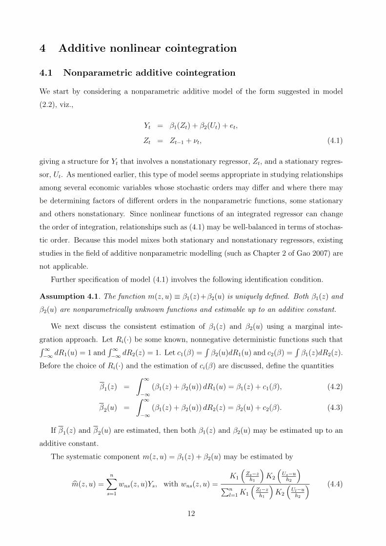
4 Additive nonlinear cointegration

4.1 Nonparametric additive cointegration

We start by considering a nonparametric additive model of the form suggested in model

(2.2), viz.,

Yt = β1(Zt) + β2(Ut) + et,

Zt = Zt−1 + νt, (4.1)

giving a structure for Yt that involves a nonstationary regressor, Zt, and a stationary regres-

sor, Ut. As mentioned earlier, this type of model seems appropriate in studying relationships

among several economic variables whose stochastic orders may differ and where there may

be determining factors of different orders in the nonparametric functions, some stationary

and others nonstationary. Since nonlinear functions of an integrated regressor can change

the order of integration, relationships such as (4.1) may be well-balanced in terms of stochas-

tic order. Because this model mixes both stationary and nonstationary regressors, existing

studies in the field of additive nonparametric modelling (such as Chapter 2 of Gao 2007) are

not applicable.

Further specification of model (4.1) involves the following identification condition.

Assumption 4.1. The function m(z, u) ≡ β1(z)+β2(u) is uniquely defined. Both β1(z) and

β2(u) are nonparametrically unknown functions and estimable up to an additive constant.

We next discuss the consistent estimation of β1(z) and β2(u) using a marginal inte-

gration approach. Let Ri(·) be some known, nonnegative deterministic functions such that∫∞−∞ dR1(u) = 1 and

∫∞−∞ dR2(z) = 1. Let c1(β) =

∫β2(u)dR1(u) and c2(β) =

∫β1(z)dR2(z).

Before the choice of Ri(·) and the estimation of ci(β) are discussed, define the quantities

β1(z) =

∫ ∞−∞

(β1(z) + β2(u)) dR1(u) = β1(z) + c1(β), (4.2)

β2(u) =

∫ ∞−∞

(β1(z) + β2(u)) dR2(z) = β2(u) + c2(β). (4.3)

If β1(z) and β2(u) are estimated, then both β1(z) and β2(u) may be estimated up to an

additive constant.

The systematic component m(z, u) = β1(z) + β2(u) may be estimated by

m(z, u) =n∑s=1

wns(z, u)Ys, with wns(z, u) =K1

(Zs−zh1

)K2

(Us−uh2

)∑n

l=1K1

(Zl−zh1

)K2

(Ul−uh2

) (4.4)

12

in which Ki(·) and hi are as in (3.3). We then estimate β1(z) and β2(u) by

β1(z) =

∫ ∞−∞

m(z, u) dR1(u) and β2(u) =

∫ ∞−∞

m(z, u) dR2(z). (4.5)

The following asymptotic results for the estimation of (4.1) are established for the case

where Ut is a stationary time series.

Theorem 4.1. Let Assumptions 4.1, A.1(i)–(iv), A.2(ii)(iii), A.3 and A.4 hold. Let dx = 2

and Xt ≡ 1 hold in (1.1) and the component functions of the model (4.1) be estimated as in

(4.5).

(i) If, in addition,√n h31 = O(1) and

√n h1h

2du2 = O(1), then as n→∞

B−11n (z)(β1(z)− β1(z)− c1(β)

)→D N(0, σ2

e), (4.6)

where B21n(z) =

∑ns=1B

21ns(z) with B1ns(z) =

∫∞−∞wns(z, u)dR1(u). The asymptotic form of

B21n(z) is given by

B21n(z) =

1√n h1

C1(K)

LB(1, 0)π1 (1 + oD(1)), (4.7)

where C1(K) =∫K2

1(x)dx and π1 =∫ r21(u)

p(u)du is the same as in Assumption A.4(ii).

(ii) If, in addition,√n h3du2 = O(1) and

√n hdu2 h

21 = O(1), then as n→∞

B−12n (u)(β2(u)− β2(u)− c2(β)

)→D N(0, σ2

e), (4.8)

where B22n(u) =

∑ns=1B

22ns(u) with B2ns(u) =

∫∞−∞wns(z, u)dR2(z). The asymptotic form of

B22n(u) is given by

B22n(u) =

1√n hdu2

C2(K)

LB(1, 0)π2 (1 + oP (1)), (4.9)

where C2(K) =∫K2

2(x)dx and π2 =∫r22(z)dz is the same as in Assumption A.4(ii).

Corollary 4.1. (i) Let the conditions of Theorem 4.1(i) hold. If, in addition, c1(β) = 0,

then as n→∞B−11n (z)

(β1(z)− β1(z)

)→D N(0, σ2

e). (4.10)

(ii) Let the conditions of Theorem 4.1(ii) hold. If, in addition, c2(β) = 0, then as n→∞

B−12n (u)(β2(u)− β2(u)

)→D N(0, σ2

e). (4.11)

Model (2.4) takes a special case of (4.1) of the form

Yt = β1(Zt) + β2(Ut) + et,

Zt = Zt−1 + νt with Ut = νt, (4.12)

13

where there is high correlation between the nonstationary regressor Zt and stationary re-

gressors Ut = Zt − Zt−1 that is induced by the specification Ut = νt. Corollary 4.2 below

shows that both functions β1(·) and β2(·) may still be consistently estimated. As discussed

in the proof given in Appendix B, this is due to the fact that the standardized variate 1√tZt

and Ut are asymptotically uncorrelated when t→∞.

Corollary 4.2. Let the conditions of Theorem 4.1 hold. Then the conclusions of Theorem

4.1 remain true for model (4.12).

Remark 4.1. Theorem 4.1 and Corollaries 4.1–4.2 show that the functions β1(·) and β2(·) are

consistently estimable. In addition, Theorem 4.1(ii) shows that the convergence rate of β2(·)

is

(√√nhdu2

)−1, which is slower than the conventional rate

(√nhdu2

)−1for the stationary

case. As discussed following Theorem 3.1, this difference is due to the nonstationarity of Zt

which impacts the convergence rate of the joint nonparametric estimator (4.4) and thereby

that of the estimator of β2(·) even though the associated regressor Ut in this function is itself

stationary.

4.2 Semiparametric additive cointegration

We now focus on models (2.6) and (2.7) and discuss the identifiability and estimability of the

unknown parameters and functions in these semiparametric models. To open discussion and

present the motivating ideas we consider a semiparametric time series model of the partial

linear form

Yt = V ′t β + β1(Zt) + et, (4.13)

where Vt = X1t in model (2.6) and Vt = Zt in model (2.7).

To begin, suppose for the moment that Vt and Zt are both stationary. Accordingly, let

H(z) = E[Vt|Zt = z]. In the case where H(z) is a smooth function and the covariance

matrix Σ = E[(Vt − E [Vt|Zt]) (Vt − E [Vt|Zt])′

]is positive definite, both β and β1(·) can be

semiparametrically estimated as in the existing literature by projecting out the nonparamet-

rically fitted conditional expectations (see, for example, Robinson 1988; Hardle, Liang and

Gao 2000; Gao 2007; Li and Racine 2007; Terasvirta, Tjøstheim and Granger 2010). In the

case where Vt and Zt are highly correlated as they may be in models (2.6) and (2.7) with

nonstationarity present, this conventional semiparametric approach can break down asymp-

totically because of potential singularity in the asymptotic moment matrix. We therefore

examine a direct approach to fitting (4.13) that takes into account the effects of nonstation-

arity on the model components.

14

Suppose we treat β as the parameter of interest in (4.13) and β1(·) as a nuisance parameter

so that the nonparametric term is absorbed into the disturbance as random noise. If Vt

and Zt were both stationary and the model itself were a linear model, then minimizing

E([Yt − V ′t b]

2) leads to the regression coefficient b = (E [V1V′1 ])−1 E [V1Y1] which equals β

under

E [V1β1(Z1)] = 0, and E [V1e1] = 0 (4.14)

the first part of which implies under ergodicity 1n

∑nt=1 Vtβ2(Zt) →P 0. So (4.14) is an

orthogonality condition which ensures that β is identifiable and estimable in the stationary

case. These considerations motivate the use of the orthogonality condition:

1

n

n∑t=1

Vtβ1(Zt) = OP (1) (4.15)

for the identification and estimability of β in the nonstationary case. To derive a more

explicit condition that reduces to (4.15), we consider the explicit case where Xt = Xt−1 +µt

and Zt = Zt−1 + νt. Without loss of generality, we here assume that X1t follows the same

model as Xt. Let dn =√n, xtn = Xt√

nand ztn = Zt√

n. Then, analogous to the proof of Lemma

A.5 in Appendix A, when dz = 1 we have the following limit behaviour as n→∞

1

n

n∑t=1

Xtβ1(Zt) =dnn

n∑t=1

(xtn) β1(dnztn)→D

∫ 1

0

Bµ(r)dLBν (r, 0) ·∫ ∞−∞

β1(z)dz,

1√n

n∑t=1

Ztβ1(Zt) =dnn

n∑t=1

(dnztn) β1(dnztn)→D LBν (1, 0) ·∫ ∞−∞

zβ1(z)dz, (4.16)

where the limits exist under the integrability conditions of Assumption 4.2 below. The

orthogonality conditions now follow directly from (4.16). As n→∞, we have

1

n

n∑t=1

Xtβ1(Zt) =1√n· 1√

n

n∑t=1

Xtβ1(Zt) = OP (1),

1

n

n∑t=1

Ztβ1(Zt) =1√n· 1√

n

n∑t=1

Ztβ1(Zt) = oP (1). (4.17)

Assumption 4.2. (i) Let β1(z) in model (2.6) be continuous in z and both β1(z) and β21(z)

be integrable. In addition,∫β1(z)dz 6= 0.

(ii) Let β1(z) in model (2.7) be continuous in z and both zβ1(z) and z2β21(z) be integrable.

In addition,∫zβ1(z)dz 6= 0.

Under Assumption 4.2, both β in model (2.6) and θ in model (2.7) are uniquely identifi-

able and consistently estimable by

β =

(n∑t=1

X1tX′1t

)−1 n∑t=1

X1tYt and θ =

(n∑t=1

ZtZ′t

)−1 n∑t=1

ZtYt. (4.18)

15

The nonparametric component β1(z) in these two models may respectively be estimated by

β1(z) =n∑t=1

wnt(z)(Yt −X ′1tβ

)for model (2.6),

β1(z) =n∑t=1

wnt(z)(Yt − Z ′tθ

)for model (2.7), (4.19)

where wnt(z) = K1

(Zt−zh1

)/∑n

s=1K1

(Zs−zh1

), in which K1 and h1 are assumed to satisfy the

following conditions.

Assumption 4.3. (i) There exists a real function L(u, v) such that

|β1(v + h1u)− β1(v)| ≤ hL(u, v)

for all u ∈ R = (−∞,∞) and∫K1(u)L(u, v)du <∞ for each given v.

(ii) The probability kernel function K1(u) satisfies∫uK1(u)du = 0,

∫u2K1(u)du <∞ and∫

K21(u)du <∞.

(iii) The bandwidth h1 satisfies h1 → 0,√nh1 →∞ and

√nh31 → 0.

We are now ready to establish the following main results on the limit theory for the

estimates of the parametric and nonparametric components in models (2.6) and (2.7). Proofs

are in Appendix B.

Theorem 4.2. (i) Let Assumptions 4.2(i) and A.1(i)(ii)(iii) hold. Then, as n→∞

n(β − β

)→D

(∫ 1

0

Bµ(r)Bµ(r)′dr

)−1×(∫ 1

0

Bµ(r)dBe(r) +

∫ 1

0

Bµ(r)dLBν (r, 0) ·∫ ∞−∞

β1(z)dz

), (4.20)

where Be(r) is the Brownian motion limit of standardized partial sums (n−1/2∑bnrc

t=1 et) of

et.

(ii) If, in addition, Assumption 4.3 holds, then as n→∞√√√√ n∑t=1

K1

(Zt − zh1

) (β1(z)− β1(z)

)→D N

(0, σ2

1(K1)), (4.21)

where σ21(K1) = σ2

e ·∫K2

1(u)du.

Theorem 4.3. (i) Let Assumptions 4.2(ii) and A.1(i)(ii)(iii) hold. Then, under Xt ≡ 1,

we have as n→∞

n(θ − θ

)→D

(∫ 1

0

Bν(r)Bν(r)′dr

)−1 ∫ 1

0

Bν(r)dBe(r). (4.22)

16

(ii) If, in addition, Assumption 4.3 holds, then we have as n→∞√√√√ n∑t=1

K1

(Zt − zh1

) (β1(z)− β1(z)

)→D N

(0, σ2

1(K1)). (4.23)

Theorem 4.2(i) shows that there is a kind of bias term involved in (4.20) when∫β1(z)dz 6=

0. By contrast, Theorem 4.3(i) shows that such a bias term disappears in the case of Xt = Zt

even when∫zβ1(z)dz 6= 0. This is basically because Xt and Zt involved in the parametric

and nonparametric components are generated by two different integrated time series in model

(2.6), while model (2.7) involves only one integrated time series in both the parametric and

nonparametric components. Note that the bias term involved in (4.20) disappears when∫β1(z)dz = 0. Note also that Theorem 4.3(i) however remains the same when

∫zβ1(z)dz =

0. We omit the discussion for the cases of∫β1(z)dz = 0 and

∫zβ1(z)dz = 0, since the detail

is very similar.

We next consider augmented regression models of the type shown in (2.10) which involve a

parametric nonstationary component combined with a nonparametric function of stationary

variates, written in the form

Yt = Ztγ + β2(Ut) + et,

Zt = Zt−1 + νt. (4.24)

The natural approach to (4.24), given the stationary nonparametric component β2(Ut), is

to estimate γ and β2(·) by semiparametric weighted least squares. However, since Zt is

nonstationary and is correlated with Ut, existing approaches and limit theory (e.g., Robinson

1988; Hardle, Liang and Gao 2000) are not directly applicable.

Let α = E [β2(Ut)] and ηt = β2(Ut)− α + et, so that (4.24) may be written as

Yt = α + Ztγ + ηt,

Zt = Zt−1 + νt. (4.25)

This formulation suggests that in (4.25) the parameter γ can be estimated by least squares,

giving

γ =

(n∑t=1

Z2t

)−1 n∑t=1

ZtYt, (4.26)

where Zt = Zt − n−1∑n

s=1 Zs and Yt = Yt − n−1∑n

s=1 Ys. The unknown function β2(u) is

then estimated by kernel regression on the residuals, leading to

β2(u) =n∑t=1

Wnt(u) (Yt − Ztγ) , (4.27)

17

where Wnt(u) = K2

(Ut−uh2

)/∑n

s=1K2

(Us−uh2

).

The limit theory for the estimates(γ, β2(u)

)obtained in this way is given in Theorem

4.4 below, for which we use the following conditions.

Assumption 4.4. (i) Suppose that β2(u) is twice differentiable and that the second deriva-

tive, β(2)2 (u), is continuous with

∫∞−∞

∣∣∣β(2)2 (u)

∣∣∣ p(u) <∞, where p(u) is the marginal density

of Ut.

(ii) K2(u) is a probability kernel with∫uK2(u)du = 0,

∫u2K2(u)du <∞ and

∫K2

2(u)du <

∞.

(iii) The bandwidth h2 satisfies h2 → 0, nhdu2 →∞ and√nh42 = O(1).

Theorem 4.4. (i) Let Assumptions A.1(i)(ii)(iii) hold. Then, for model (4.25), we have as

n→∞

n (γ − γ)→D

(∫ 1

0

Bν(r)2

)−1 ∫ 1

0

Bν(r)dBη(r), (4.28)

where Bη(r) is defined as the weak limit of Πn(r) = 1√n

∑bnrct=1 ηt ⇒D Bη(r) on the Skorohod

space D[0, 1] and Bν(r) = Bν(r)−∫ 1

0Bν(s)ds.

(ii) If Assumption 4.4 also holds, then as n→∞√nhdu2

(β2(u)− β2(u)

)→D N

(0, σ2

2(K2)), (4.29)

where σ22(K2) = σ2

e ·∫K2

2(u)du.

Remark 4.2. Theorems 4.2 and 4.3 show that the usual order n convergence rate of linear

cointegration is achievable in the semiparametric case as long as the identification condition

in Assumption 4.2 holds and direct least squares regression in (4.25) is used. Other methods,

such as fully modified least squares (Phillips and Hansen, 1990) may be employed in this

model to remove second order bias effects (arising from serial dependence in ηt = β2(Ut) −α+ et and endogeneity in Zt) in the usual way and to conduct pivotal inference on γ. These

methods are standard and do not need to be detailed here. However, as shown in Example

5.3 below, the more conventional semiparametric least squares estimator of γ in (4.24) can

have a much slower rate of convergence than the order n rate in some nonstationary models

when Assumption 4.2(ii) does not hold.

5 Examples of implementation

This section provides three examples of implementation with specific parameter settings.

The first focuses on a varying–coefficient model. The second considers some particular cases

18

of a nonparametric additive model. Some versions of semiparametric cointegrating models

are discussed in the third example.

Example 5.1. Consider a varying–coefficient model of the form

Yt = Xt β(Zt, Ut) + et, t = 1, 2, · · · , n,

Xt = Xt−1 + µt with µt = 0.5µt−1 + εt,

Zt = Zt−1 + νt with νt = −0.5νt−1 + εt,

β(z, u) =z

(1 + z2)32

+ u, (5.1)

where X0 = Z0 = 0, µ0 = ν0 = 0, et = εt+1 and {εt}iid∼ N [0, 1]. We take the following two

cases:

Case A : Ut = νt Case B : Utiid∼ U [0, 1],

where U [0, 1] denotes the uniform distribution on [0, 1].

The function β(·, ·) is estimated by local level regression as

β(z, u;h1, h2) =

(n∑t=1

X2tK1

(Zt − zh1

)K2

(Ut − uh2

))−1

×

(n∑t=1

XtYtK1

(Zt − zh1

)K2

(Ut − uh2

)), (5.2)

for certain bandwidth choices (h1, h2). To select (h1, h2) we first introduce the leave–one–out

estimator of β(z, u) which we write in the form β(−t)(z, u). We then define the leave–one–out

cross–validation (CV) function as

CV(h1, h2) =1

n

n∑t=1

(Yt −Xt β(−t)(Zt, Ut)

)2. (5.3)

An optimal bandwidth value for (h1, h2) is chosen according to the rule

CV(h1, h2) = minh1,h2∈H2n

CV(h1, h2), (5.4)

where H2n is of the form [n−1, n−1+c1 ] × [n−1, n−1+c2 ], in which each 0 < ci < 1 is chosen

such that each of (h1, h2) is achievable and locally unique. With this bandwidth choice, the

function β(·, ·) is estimated by

β(z, u) = β(z, u; h1, h2). (5.5)

We perform a small simulation experiment to evaluate the performance characteristics of

β(z, u) for sample sizes n = 201, 551, 901, and 1501. Finite sample performance is assessed

19

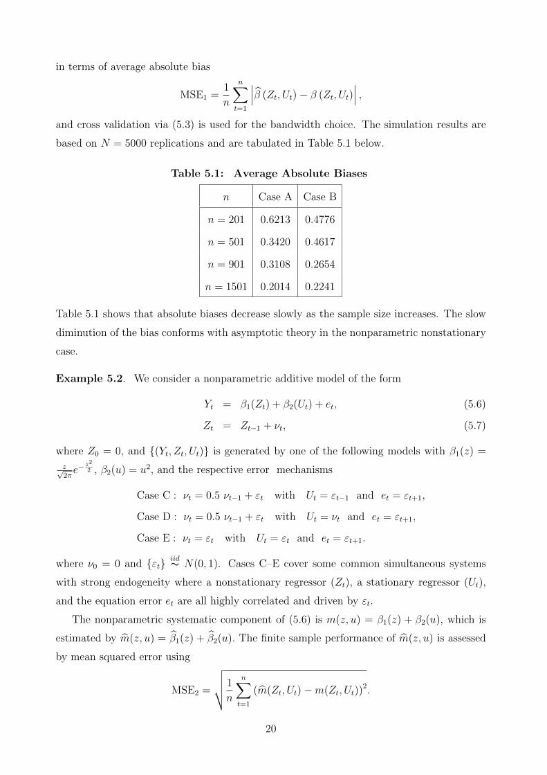
in terms of average absolute bias

MSE1 =1

n

n∑t=1

∣∣∣β (Zt, Ut)− β (Zt, Ut)∣∣∣ ,

and cross validation via (5.3) is used for the bandwidth choice. The simulation results are

based on N = 5000 replications and are tabulated in Table 5.1 below.

Table 5.1: Average Absolute Biases

n Case A Case B

n = 201 0.6213 0.4776

n = 501 0.3420 0.4617

n = 901 0.3108 0.2654

n = 1501 0.2014 0.2241

Table 5.1 shows that absolute biases decrease slowly as the sample size increases. The slow

diminution of the bias conforms with asymptotic theory in the nonparametric nonstationary

case.

Example 5.2. We consider a nonparametric additive model of the form

Yt = β1(Zt) + β2(Ut) + et, (5.6)

Zt = Zt−1 + νt, (5.7)

where Z0 = 0, and {(Yt, Zt, Ut)} is generated by one of the following models with β1(z) =

z√2πe−

z2

2 , β2(u) = u2, and the respective error mechanisms

Case C : νt = 0.5 νt−1 + εt with Ut = εt−1 and et = εt+1,

Case D : νt = 0.5 νt−1 + εt with Ut = νt and et = εt+1,

Case E : νt = εt with Ut = εt and et = εt+1.

where ν0 = 0 and {εt}iid∼ N(0, 1). Cases C–E cover some common simultaneous systems

with strong endogeneity where a nonstationary regressor (Zt), a stationary regressor (Ut),

and the equation error et are all highly correlated and driven by εt.

The nonparametric systematic component of (5.6) is m(z, u) = β1(z) + β2(u), which is

estimated by m(z, u) = β1(z) + β2(u). The finite sample performance of m(z, u) is assessed

by mean squared error using

MSE2 =

√√√√ 1

n

n∑t=1

(m(Zt, Ut)−m(Zt, Ut))2.

20

Bandwidth selection is performed by cross validation as in (5.3) and the simulation results

reported in Table 5.2 below are based on N = 5000 replications.

Table 5.2: Average Mean Squared Error

n Case C Case D Case E

n = 201 0.0175 0.0312 0.0169

n = 501 0.0162 0.0284 0.0148

n = 901 0.0148 0.0275 0.0137

Table 5.2 shows that the proposed estimator performs adequately even in the presence of

strong endogeneity among both stationary and nonstationary variables in this model. Again,

the mean squared error of the nonparametric estimator declines slowly with n.

Example 5.3. We consider a regression model that involves a nonstationary regressor and

takes the partially linear form

Yt = Zt θ + β1(Zt) + et, (5.8)

Zt = Zt−1 + νt, (5.9)

where the initialization Z0 = 0 and various functional forms for β1(·) and probabilistic

structures for {νt} are explored. This type of model might be used as a partially linear

predictive regression model when Zt is adapted to the past. We examine two approaches

to estimating model (5.8). The first involves direct estimation and subsequent elimination

of the linear cointegrating component. The second follows the conventional semiparametric

approach of first eliminating the functional component by nonparametric regression. It will

become apparent that these approaches have very different properties in a model such as

(5.8) and (5.9) where the regressor is nonstationary.

The first approach proceeds on the presumption of a strong signal in the regressor Zt

from the stochastic trend (5.9) and the presence of a nonlinear integrable function β1 ∈ L1

that attenuates the effects of large Zt. The coefficient θ of the linear cointegrating term in

(5.8) may then be estimated directly by least squares as

θ = (Z ′Z)−1Z ′Y, (5.10)

where Z ′ = (Z1, · · · , Zn) and Y ′ = (Y1, · · · , Yn). The unknown function β1 can subsequently

be estimated using nonparametric regression on the parametric residuals to capture any

21

potential nonlinear effects as follows

β1(z, h3) =n∑s=1

Wns(z;h3)(Ys − Zsθn

), (5.11)

where Wns(z;h3) = K1

(Zs−zh3

)/

n∑l=1

K1

(Zl−zh3

). The bandwidth h3 is selected by minimizing

the cross validation criterion

CV(h3) =1

n

n∑t=1

(Yt − θnZt − β1,(−t)(Zt;h3)

)2, (5.12)

with β1,(−t)(Zt, h3) =∑n

s=1, 6=tK1

(Zs−Zth3

)(Ys − Zsθ

)/

n∑k=1,6=t

K1

(Zk−Zth3

)such that

CV(h3) = minh∈H3n

CV(h3), (5.13)

in which H3n has the form [n−1, n−1+c3 ] with each 0 < c3 < 1 chosen so h3 is achievable and

locally unique. This process leads to the following estimate of β1 as

β1(z) = β1(z; h3). (5.14)

The second approach follows conventional semiparametric practice of eliminating the non-

parametric component and then proceeding with a direct regression for the linear component

using the nonparametric residuals. Accordingly, we define the following leave–one–out non-

parametric estimators

Ψt(Zt) =n∑

s=1, 6=t

W (−t)ns (Zt)Ys and Γt(Zt) =

n∑s=1,6=t

W (−t)ns (Zt)Xs, (5.15)

where W(−t)ns (Zt) = K1

(Zs−Zth4

)/

n∑k=1, 6=t

K1

(Zk−Zth4

)and h4 is a bandwidth parameter. Let

the residuals from these regressions be Yt =(Yt − Ψ(Zt)

)and Zt =

(Zt − Γ(Zt)

). We then

consider the following approximate system that is induced after (semiparametric) elimination

of the function β1

Yt = θ Zt + error. (5.16)

The leave–one–out semiparametric least squares (SLS) estimator of θ is obtained by linear

regression on this approximate system leading to

θ(h4) = (Z ′Z)−1Z ′Y , (5.17)

where Z ′ = (Z1, · · · , Zn) and Y ′ = (Y1, · · · , Yn) for some bandwidth h4. Next we define the

leave–one–out cross–validation (CV) function as

CV(h4) =1

n

n∑t=1

(Yt − θZt

)2, (5.18)

22

and an optimal bandwidth value for h4 is chosen such that

CV(h4) = minh∈H4n

CV(h4), (5.19)

where H4n is of the form [n−1, n−1+c4 ], in which each 0 < c4 < 1 is chosen such that each

of h4 is achievable and locally unique. The parameter θ is then estimated by θ ≡ θ(h4).

Estimation of β1 follows by local level regression as

β1(z) =n∑s=1

Wns(z; h4)(Ys − Zs θ

), (5.20)

where Wns(z;h4) = K1

(Zs−zh4

)/

n∑k=1

K1

(Zk−zh4

).

We perform a small simulation exercise to assess the finite–sample performance of θ

and θ. The relevant asymptotics for θ are given in Theorem 4.3, where it is shown that θ is

asymptotically mixed normal with convergence rate n. By contrast, θ appears to have a slow

rate of convergence, as evidenced by the large variances and mean squared errors reported

in the simulations below. A rigorous asymptotic treatment of this case presents substantial

challenges, and only the following heuristic analysis is attempted here.

The intuition is worth describing. In the first approach, the direct linear cointegrating

regression (5.10) preserves the signal strength of the unit root process Zt, thereby producing

an O (n) convergence rate because the effect of the misspecification from ignoring the nonlin-

ear component is negligible when β1 ∈ L1 since n−1n∑k=1

Ztβ1(Zt) = op (1) under very general

assumptions (see Phillips, 2009). In the second approach, the dependent variable Yt and lin-

ear regressor Zt are both effectively ‘detrended’ using nonparametric leave-one-out regression

(5.15), producing residuals Yt and Zt. The effect of this detrending on Zt is analogous to a

nonparametric autoregression of Zt on Zt−1, which is consistent (Wang and Phillips, 2009a)

and, in the present case, fits the trajectory of Zt (as described in Phillips, 2009), and whose

residuals therefore behave more like an I (0) variate than an I (1) variate. The resulting

second stage estimator θ(h4) of θ suffers from this semiparametric adjustment by using a

regressor with a diminished signal, leading to an estimator with a slower convergence rate or

possibly inconsistency. Hence, in the case of nonstationary semiparametric regression, con-

ventional semiparametric estimation performs a preliminary nonparametric regressions on

the dependent variable and regressor which acts as a form of stochastic detrending of those

variables that reduces their signal strength. The secondary regression applies to the residu-

als from this first stage nonparametric regressions and therefore suffers the consequences of

the reduced signal strength, thereby affecting the convergence of the estimates of the linear

component.

23

Tables 5.3 and 5.4 below provide simulation findings that support this distinction between

the two estimators. The simulation uses the following generating mechanisms involving two

different L1 functions β1 :

Case F : νt = 0.5 νt−1 + εt with et = εt+1 and β1(z) =1√2πe−

z2

2 ,

Case G : νt = 0.5 νt−1 + εt with et = εt+1 and β1(z) =1

(1 + z2)32

,

where ν0 = 0 and {εt}iid∼ N [0, 1]. We assess finite sample performance in terms of bias,

standard deviation and mean square error computed as

ABS(µ) =1

N

N∑j=1

|µ(j)− θ| and STD(µ) =

√√√√ 1

N

N∑j=1

(µ(j)− µ

)2,

MSE1(β) =1

n

n∑t=1

∣∣∣β(Zt)− β(Zt)∣∣∣ and MSE2(β) =

√√√√ 1

n

n∑t=1

(β(Zt)− β(Zt)

)2,

where µ = θ or θ, β(·) = β1(·) or β1(·), µ = 1N

∑Nj=1 µ(j), and µ(j) is the estimator at the

j–th replication. The simulation results reported in Tables 5.3 and 5.4 below are based on

N = 5000 replications and provide the mean ABS and MSE outcomes.

Table 5.3: ABS and MSE Outcomes for Case F

Case A n = 201 n = 501 n = 901

ABS(θ) 0.002723 0.001032 0.000587

std(θ) 0.002541 0.000968 0.000521

ABS(θ) 0.029187 0.012981 0.0055897

std(θ) 0.098776 0.074876 0.035657

MSE1(β1) 0.121563 0.093451 0.080748

MSE2(β1) 0.141674 0.103564 0.090414

MSE1(β1) 0.654856 0.638715 0.604646

MSE2(β1) 0.914873 0.870187 0.843102

Tables 5.3 and 5.4 clearly show the superiority of the estimator θ in terms of both bias

and mean square error, at least under Assumption 4.2(ii). The semiparametric weighted

least squares estimator θ has decidedly poor performance by comparison. Similarly, the

nonparametric estimator β1 is superior to β1 in all cases and by both criteria. The usual

semiparametric estimator is therefore seen to be quite unreliable in this class of models

24

with a nonstationary regressor, even though it is commonly used in partially linear model

estimation.

Table 5.4: ABS and MSE Outcomes for Case G

Case B n = 201 n = 501 n = 901

ABS(θ) 0.003576 0.001329 0.000658

std(θ) 0.003109 0.001108 0.000529

ABS(θ) 0.034623 0.017328 0.008946

std(θ) 0.09826 0.07639 0.053879

MSE1(β1) 0.114636 0.095783 0.081793

MSE2(β1) 0.135723 0.10958 0.094764

MSE1(β1) 0.684102 0.668231 0.636728

MSE2(β1) 0.981439 0.947628 0.875682

6 Empirical application to consumption

This section provides an empirical application of the methods to explain aggregate consump-

tion behavior in the US over the period 1960 - 2009. Our primary focus in this application

is the identification and estimation of potential nonlinearities in relationships involving the

nonstationary aggregate consumption data. A secondary focus is to explore the potential

role of other macroeconomic variables like interest rates in influencing the form of the non-

stationary relationships.

We use data from the Bureau of Economic Analysis2 on the following three variables:

ct = log(consumption expenditure), it = log(disposable income), and rt = real interest rate.

Note that ct, it and rt are all real data. The data are quarterly and comprise 199 observations

over the period from the first quarter of 1960 to the last quarter of 2009. The real interest

rate variable is measured by subtracting the ex post inflation rate over the following quarter

from the nominal interest rate. The data are plotted in Fig. 1. The histograms shown on

the axis borders provide crude estimates of the local time spent at various levels by the series

over the period 1960Q1-2009Q4. The strong trend component in ct and it is reflected in the

near uniform local time estimates for these series in comparison with rt (c.f., Phillips, 2001b,

25

1960 1970 1980 1990 20007

8

9

10

1960 1970 1980 1990 20007.5

8

8.5

9

9.5

1960 1970 1980 1990 2000

0

0.05

0.1

7.5 8 8.5 9

4

6

8

10

Yt

7.5 8 8.5 9

4

6

8

10

Xt

0 0.05 0.10

5

10

15

20

Zt

Yt: log(PCE) Xt: log(DPI)

Zt: RIR

Figure 1. The top panel gives the plots of Yt = ct, Xt = it and Zt, respectively, and the

bottom panel gives their corresponding local–time densities.

2005).

Transforming to the notation of the paper we set Yt = ct, Xt = it, and Zt = rt. A

convenient starting point is the prototype fixed parameter consumption function

Yt = α + βXt + et, (6.1)

whose differenced form

Yt − Yt−1 = β (Xt −Xt−1) + et − et−1 ≡ β (Xt −Xt−1) + εt (6.2)

is the basis for many empirical models that are common in the literature (e.g., Campbell

and Mankiw 1990; Campbell, Lo and MacKinlay 1997).

The methods developed in the paper can be used to check whether a fixed parameter

model such as (6.2) is supported empirically against more general functional specifications.

There is a growing literature (see, for example, Gylfason, 1981; Faff and Brooks, 1998;

Hahm and Steigerwald, 1999; Cai, Li and Park, 2009; Xiao, 2009) to support alternative

formulations that treat the propensity to consume parameter β as a function of certain

covariates. Among other possibilities, polynomial functions have often been suggested as

flexible functional forms for variable coefficients such as β(·) – see, for example, Faff and

Brooks (1998). Underlying such formulations is a Hall–type (1978) consumption model with

varying coefficients of the form

Yt = α(Zt−1) + β(Zt−1)Yt−1 + ζt, (6.3)

2The data are available at: http://www.bea.gov.

26

where both α(z) and β(z) are unknown functions of z, and ζt is an error process. This model

may be fitted and analyzed using the methods of the present paper. Specific functional forms

may then be tested against (6.3).

Let K(·) be a probability kernel and h the bandwidth. Functions α(z) and β(z) can be

nonparametrically estimated by minimising

1

n

n∑t=1

(Yt − α(z)− β(z)Yt−1)2K

(Zt−1 − z

h

)(6.4)

over α = α(z) and β = β(z), leading to the nonparametric estimates

β(z) =

∑ns=1

∑nt=1 YsYs−1Kst(z)−

∑ns=1

∑nt=1 YsYt−1Kst(z)∑n

s=1

∑nt=1 Y

2s−1Kst(z)−

∑ns=1

∑nt=1 Ys−1Yt−1Kst(z)

, (6.5)

α(z) =

∑nt=1K

(Zt−1−z

h

)(Yt − β(z)Yt−1

)∑n

t=1K(Zt−1−z

h

) , (6.6)

where Kst(z) = K(Zt−1−z

h

)K(Zs−1−z

h

).

An application of the nonparametric test proposed in Gao et al (2009a) to test the null

hypothesis H0 : α(z) = α0 and β(z) = β0 ≡ 1 produces a p–value of 0.1874. This test

suggests that it may not be unreasonable to assume that Yt follows a unit–root structure of

the form Yt = α0 + Yt−1 + ζt, supporting the original analysis in Hall (1978).

To use the explicit framework of the present paper with potentially nonlinear nonsta-

tionary regressors, we propose a varying–coefficient model of the form

Yt = β(Zt)Xt + et,

Xt = L1(Xt−1) + µt,

Zt = L2(Zt−1) + νt, (6.7)

where β(·) and Li(·) are all unknown functions. Taking this general nonlinear framework as

a starting point, we proceed to evaluate whether the data exhibit any unit root structure by

using the nonparametric test proposed in Gao et al (2009a) for checking empirical support

in the data for the null hypothesis H0 : P (L1(Xt−1) = Xt−1) = P (L2(Zt−1) = Zt−1) = 1.

The respective p–value outcomes of 0.2316 and 0.1092 imply that it is reasonable to assume

that both Xt and Zt follow the unit root structure given in model (1.1). This empirical

simplification along with model (6.7) then suggests the simpler system

Yt = β(Zt)Xt + et,

Xt = Xt−1 + µt,

Zt = Zt−1 + νt,

E[et] = E[µt] = E[νt] = 0, (6.8)

27

To allow for endogeneity between et and (Xt, Zt), we decompose et as et = λ(µt, νt) + εt

so that E[εt|µt, νt] = 0. Let Ut = (µt, νt)′, Xt = (Xt, 1)′ and β(Zt, Ut) = (β(Zt), λ(Ut))

′.

Accordingly, we can rewrite (6.8) in augmented regression format as

Yt = X′tβ(Zt, Ut) + εt = Xtβ(Zt) + λ(Ut) + εt,

Xt = Xt−1 + µt,

Zt = Zt−1 + νt, (6.9)

which falls within the class of varying coefficient models studied in this paper. Accordingly,

using (3.4) we have

β(z, u) =

β(z)

λ(u)

=

(n∑t=1

XtX′tK1

(Zt − zh1

)K2

(Ut − uh2

))−1

×

(n∑t=1

XtYtK1

(Zt − zh1

)K2

(Ut − uh2

))

=

∑nt=1X

2tK1

(Zt−zh1

)K2

(Ut−uh2

) ∑nt=1XtK1

(Zt−zh1

)K2

(Ut−uh2

)∑n

t=1XtK1

(Zt−zh1

)K2

(Ut−uh2

) ∑nt=1K1

(Zt−zh1

)K2

(Ut−uh2

)−1

×

∑nt=1XtYtK1

(Zt−zh1

)K2

(Ut−uh2

)∑n

t=1 YtK1

(Zt−zh1

)K2

(Ut−uh2

) . (6.10)

The asymptotic theory developed in Theorem 3.2 is then applicable to the nonparametric

component estimates(β(z), λ(u)

)of β(Zt, Ut).

The plot of β(z) shown in Fig. 2 over z ∈ (−0.02, 0.1) suggests that the function β (z)

may be reasonably approximated by a second–order polynomial function of the following

form, at least over this part of the sample space,

β2(z) = β0 + β1 z + β2 z2. (6.11)

The parameters β0, β1 and β2 may be estimated through (6.9) when β(z) is replaced by

the specification (6.11). Since E [λ(µt, νt)] = 0, we apply the approach given in (4.24)–

(4.27) to estimate (β0, β1, β2) by (β0, β1, β2) minimizing∑n

t=1 (Yt −Xtβ2(Zt))2. The unknown

complementary function λ(Ut) is then estimated by λ(u) =∑ns=1K2

(Us−uh2

)(Ys−Xsβ2(Zs))∑n

s=1K2

(Us−uh2

) , in

which K2(v) = 1√2πe−

v2

2 and h2 is chosen by semiparametric cross–validation as in Section 5

above.

The fitted parametric model is

β2(z) = β0 + β1z + β2z2, (6.12)

28

where β0 = 0.6233, β1 = −0.4293 and β2 = 1.5725. A t–test confirms that all these

coefficients are significant with p–values close to zero3. An application of the specification

test proposed in Gao, Tjøstheim and Yin (2012) to test this parametric specification against

a general nonparametric alternative produces a p–value of 0.2317. This test outcome suggests

that the quadratic approximation β2(z) of β(z) may be reasonable over this particular region

of the sample space. A simpler linear parametric form produced the fitted function

β1(z) = 0.6165− 1.901z. (6.13)

As in the case of (6.12), a t–test shows that the coefficients are all significant.

The nonparametric estimate β(z) is shown in Figure 2 against plots of the parametric

estimates β1(z) and β2(z). These plots corroborate the empirical test results, indicating that

the functional slope coefficient β(z) in (6.8) can be approximately treated as a second order

polynomial function of Zt rather than as a constant parameter for values of the real interest

rate in the region (−0.02, 0.1). Fixed coefficient models such as (6.2) do not seem to be

supported against general nonlinear varying coefficient alternatives for these data.

-0.02 0 0.02 0.04 0.06 0.08 0.10.58

0.59

0.6

0.61

0.62

0.63

0.64

Zt

-(Zt)

-1(Zt)

-2(Zt)

Figure 2. The curve in blue is the nonparametric estimate; the dot lines in red represent

the second–order polynomial; and the dot lines in black denote the linear line.

This empirical implementation of kernel nonparametrics uses cross validation based

choices of the bandwidths as in (5.3) and (5.4). Since the vector of regressors Ut involved in

3Conventional t–tests are robust to this type of parametric regression under nonstationarity, being equiv-

alent to those from a standardised (weak trend) model of the form Yt = Xd,tβ2(Zd,t) + et, where Xd,t = Xt√n

and Zd,t = Zt√n, and giving the same p–values.

29

the nonparametric kernel estimation (6.9) is stationary, the asymptotic consistency of θ(z)

follows in a similar way to Theorem 4.4, provided the parametric specification is correct.

These asymptotic results therefore justify the use of the nonparametric and semiparametric

methods in the empirical analysis in the presence of nonstationary time series regressors and

varying coefficients.

7 Conclusion and further discussion

This paper has focused on varying coefficient models of the type (1.1) that include a wide

range of related specifications such as multivariate nonparametric models of the form (2.1)

and partial linear models such as those in (2.6) - (2.8). Many of these models are now used in

empirical research with cross section data under independence assumptions. But the models

are also relevant in time series contexts in econometrics where stochastic nonstationarity is

a feature of much economic and financial data. The model constructions we have used here

allow for intrinsically nonstationary specifications in the data generating mechanisms within

a wide class of nonparametric and semiparametric regressions. Asymptotic theory for all

these regressions is developed as well as some new methods of estimation for particular cases

that take advantage of the data nonstationarity. These results will be of use to practitioners

in time series econometrics who want to consider many different alternatives to linear speci-

fications, including varying coefficient models and additive nonlinear nonstationary systems.

Some developments of the methods and results of the paper are possible and desirable.

In an early draft of this paper (Gao and Phillips, 2012), we also considered models such as

(1.1) in cases where Xt = ft+µt and Zt = gt+νt, with ft and gt being unknown deterministic

functions of t. For such specifications and under certain conditions, the estimation theory

corresponds to the case where Xt and Zt are stationary. Rather more generally, the proposed

procedures and limit theory may be extended to deal with models of the type

Yt = X ′t β(Zt, Ut) + et,

Xt = Xt−1 + ft + µt,

Zt = Zt−1 + gt + νt, (7.1)

where ft and gt are unknown deterministic functions of t. In this case, the variables involve

both stochastic trends and deterministic components. In such cases, it is realistic in practical

work to expect that the functional forms of the deterministic components will be unknown.

Then reparameterization, filtering, or linear regression extraction (as in Park and Phillips,

30

1988,1989) is generally not applicable for removing the trends involved in Xt and Zt without

risk of misspecification bias. Nonparametric estimation is needed to address these more

general specifications. Establishment of a limit theory in such cases depends on how the

deterministic trend components behave asymptotically. For instance, in the case where

(ft, gt) are weak trends (i.e., representable in standardized form as(f(tn

), g(tn

))for some

continuous functions (f, g)), Xt has the following asymptotic form upon restandarization

1

nXt =

1

n

t∑s=1

µs +1

n

t∑s=1

f( sn

)=

1√nµt,n +

∫ tn

0

f(r)dr + o(1)

=1√nµt,n + q

(t

n

)+ o(1) = q

(t

n

)+ oP (1), (7.2)

where µt,n = 1√n

∑ts=1 µs = Op (1) and q(r) =

∫ r0f(s)ds is an accumulated trend function.

A different array specification with ft,n = n−1/2f(tn

)and gt,n = n−1/2g

(tn

), leads to an

alternate asymptotic form in which both deterministic and stochastic trends remain relevant,

viz.,

Xt√n

=1√n

t∑s=1

µs +1

n

t∑s=1

f( sn

)=

1√nµt,n +

∫ tn

0

f(r)dr+ o(1) = Bµ

(t

n

)+ q

(t

n

)+ oP (1),

in a suitable probability space where µbnrc,n = Bµ (r) + op (1) . For such a model, some

results corresponding to those given here seem attainable and worthy of future investigation.

Further extensions of our results to cases where the regressor Xt and functional coefficient

argument Zt have a local to unity rather than unit root structure also seem possible, following

on from recent work on nonparametric asymptotics (Wang and Phillips, 2009a).

8 Appendix A: Assumptions and proofs

8.1 Assumptions

This paper considers the case where covariates Xt and Zt are generated as integrated processes

according to

Xt = Xt−1 + µt and Zt = Zt−1 + νt, t = 1, 2, · · · , n, (7.1)

where X0 = Z0 = OP (1). Let dµ, dν = 1 and du be the dimensions of Xt, Zt and Ut, respectively,

duµν = du + dµ + 1 and {ξi : −∞ < i < ∞} be a vector of duµν–dimensional independent and

identically distributed (iid) random variables.

Let Wt = (µ′t, νt, U′t)′. Suppose that there is a real–valued matrix of lag coefficients of the form

Cj = (cj,kl : 1 ≤ k, l ≤ duµν) such that Wt =∑∞

j=0Cjξt−j . As discussed in Remark A.2 in Appendix

A below, the main results of this paper remain true when µt and νt follow linear processes, and

31

Ut is a stationary time series generated by Ut = Λ(ξt−1, · · · , ξt−τ ; ηt), where Λ(·, · · · , ·) is a vector

function and ηt is another vector of independent and identically distributed random variables.

Throughout the paper we use ||·|| for the Euclidean norm, “⇒D” for weak convergence, “→D ”

for convergence in distribution, and “→P ” for convergence in probability.

Assumption A.1 (i) Let {ξi : −∞ < i < ∞} be a sequence of iid continuous random vectors

with E[ξ1] = 0 and positive definite matrix Σξ and finite fourth order cumulants. Let ϕ(u) be the

characteristic function of ξ1 and assume∫∞−∞ |u| |ϕ(u)| du <∞. Let the density, pξ(·), of ξ1 satisfy∫

|pξ(x+ y)− pξ(x)| dx ≤ cξ|y| for each given y and some constant cξ > 0. Let E[||ξ1||2+δ

]< ∞

for some δ > 0 satisfying 2δ2 + 4δ − 5 > 0.

(ii) The coefficients {cj,kl} satisfy∑∞

j=0 cj,klzj 6= 0 for |z| ≤ 1 and cj,kl = O

(j−λ)

as j → ∞,

where λ > 1 is chosen such that λ+ 12 > 2 + δ > 2

λ−1 with δ > 0 as in (i).

(iii) Let Ft = σ(et, · · · , e1; ξt+1, ξt, · · · , ξ−∞) be a σ–field generated {(ei, ξj) : 1 ≤ i ≤ t;−∞ <

j ≤ t + 1} with E[et|Ft−1] = 0 a.s., E[e2t |Ft−1] = σ2e a.s. and E[e4t |Ft−1

]< ∞ a.s. for all t ≥ 2,

where σ2e > 0 is some constant.

(iv) Let En(r) = 1√n

∑bnrct=1 et and Wn(r) = 1√

n

∑bnrct=1 Wt. There is a vector Brownian motion

(Be, Bw) such that (En(r),Wn(r)) =⇒D (Be(r), Bw(r)) on the Skorohod space D[0, 1]duµν+1 as

n→∞, where Bw(r) =(B′µ(r), Bν(r), B′u(r)

)′.

(v) Let {ξt} and {es} be independent for all t ≥ s+ 2.

Assumption A.2. (i) Suppose that β(z, u) is continuously differentiable in (z, u).

(ii) For i = 1, 2, let each Ki(·) be symmetric, continuous, non–negative and bounded probability

densities with∫||u||2Ki(u)du <∞ for i = 1, 2.

(iii) Let limn→∞ h1 = limn→∞ h2 = 0, limn→∞√nh1h

du2 = ∞, limn→∞

√n h51h

du2 = 0 and

limn→∞√n h1h

4+du2 = 0.

Assumption A.3. Let p(u) be the marginal density function of Ut and pτ (u, v) be the joint

density of (Ut, Ut+τ ). Suppose that p(u) is continuous in u and that pτ (u, v) is also continuous in

(u, v) uniformly in τ ≥ 1.

Assumption A.4. (i) β1(z) and β2(u) are both continuously differentiable.

(ii) R1(·) and R2(·) are continuously differentiable. For i = 1, 2, there exist bounds 0 < cimin <

cimax < ∞ such that c1min ≤ π1 ≤ c1max and c2min ≤ π2 ≤ c2max, where π1 =∫ r21(u)

p(u) du with

r1(u) = dR1(u)du and π2 =

∫r22(z)dz with r2(z) = dR2(z)

dz .

(iii) Additionally,∫ ∣∣∣β(1)1 (z)

∣∣∣ r2(z)dz <∞ and∫ ∣∣∣β(1)2 (u)

∣∣∣ r1(u)du <∞.

Since the lag coefficient matrix Cj is not necessarily diagonal, Assumption A.1(i)(ii) allows

for contemporaneous correlation between the regressors and the residuals. This joint dependence

structure allows for the presence of endogeneity and nonstationarity.

32

Remark A.1(i) Assumption A.1(i)(ii) ensures that Wt is stationary and α–mixing (see, for ex-

ample, Corollary 4 of Withers 1981; Theorem 2.1 of Pham and Tran 1985). Assumption A.1(i)(ii)

allows for correlated {Ut} and {µt, νt}, including the special case of strong endogeneity where

Ut = νt. As a result, we can have Zt − Zt−1 = Ut as mentioned in models (2.4) and (2.10) above.

Note also that Assumption A.1(i)(ii) covers the case where {Ut} is independent of {(µt, νt)}. Both

the correlated and uncorrelated cases for {Ut} and {(µt, νt)} are considered in simulations. Instead

of imposing a linear process structure, one may directly assume that Wt is a vector of station-

ary and α–mixing time series with mixing coefficient αw(·) satisfying∑∞

k=1 αδ1

2+δ1w (k) < ∞, where

δ1 > 0 is chosen such that E ||Wt||2+δ1 < ∞. In order to validate the main theorems in this case

(particularly the proof of Theorem 3.2), the extra condition is included in Assumption A.1(iv) that

Bµ(r) and Bν(r) are independent.

(ii) In applications, we may choose Ft = σ (et, · · · , e1; ξt+1, ξt, · · · , ξ−∞) generated by {(ei, ξj) :

1 ≤ i ≤ t;−∞ < j ≤ t}. In this case, Assumption A.1(v) holds if {ξs} and {et} are independent for

all s ≥ t + 1. Assumption A.1(iii)-(iv) also allows for heteroskedastic innovations et. Assumption

A.2(i)(ii) imposes some mild conditions on the kernel functions and β(z, u). Assumption A.2(iii)

imposes some technical conditions on the bandwidth parameters. The last part of Assumption

A.2(iii) links the mixing coefficient αw(·) with the bandwidths - it is verifiable and satisfied when

hi = O(n−λi

)for i = 1, 2, and (λ0, λ1, λ2) is chosen suitably such that λ1 ≥ 1

2 (λ2 − λ0). Assump-

tions A.3 and A.4 are reasonable and may be justified under more primitive conditions.

8.2 Useful lemmas

The following lemmas are needed for us to establish some useful asymptotic properties and are of

independent interest.

Let qt(u|x, z) and qt(u|z) be the conditional density functions of Ut given(Xt√t, Zt√

t

)and of Ut

given Zt√t, respectively. For i = 0, 1, let q

(i)t (u|x, z) and q

(i)t (u|z) be the i–th partial derivative with

respect to t. We then have the following lemma.

Lemma A.1. Let Assumption A.1(i)(ii) hold. As t, s→∞ and st → 0, then

(Xt√t, Zt√

t

),(Xs√s, Zs√

s

),

Ut and Us are mutually independent.

Meanwhile, we have as t→∞

q(i)t (u|x, z)→ p(i)(u) and q

(i)t (u|z)→ p(i)(u) (7.2)

for i = 0, 1, where p(u) denotes the marginal density of Ut.

Proof : Let us introduce some notation. Recall the definitions of µt, νt and Ut as given in As-

sumption A.1. Let D1 and D2 be vectors of real numbers, and D3 be a real number itself. Define

33

ut = Dτ1µt +D3νt and vt = Dτ

2Ut. It follows from Assumption A1(i)(ii) that there are coefficients

{cj : j ≥ 0} and {dj : j ≥ 0} as well as a sequence of independent and identically distributed

random variables {εi : −∞ < i <∞} such that

ut =

∞∑j=0

cjεt−j and vt =

∞∑j=0

djεt−j , (7.3)

where {εi} satisfies the same conditions that are imposed on the components of ξi in Assumption

A.1(i), and {cj : j ≥ 0} and {dj : j ≥ 0} satisfy such conditions that are imposed on {cj,kl} in

Assumption A.1(ii). In order to prove Lemma A.1, it suffices to show that ut√t, us√

s, vt and vs are

mutually independent when t, s→∞ and st → 0.

Before we prove this lemma, we point out that Lemma A.1 implies the mutual independence

between ut√t

and(us√s, vt, vs

)when t, s → ∞ and s

t → 0. As a consequence, it implies the mutual

independence between Zt and (Zs, vt, vs) when t, s→∞ and st → 0.

To simplify the notation, we assume without loss of generality that var(ut) = var(vt) ≡ 1. In

addition, we avoid involving s and t as the indices. For t > s, let Y1 =∑ti=1 ui√t

, Y2 =∑sj=1 uj√s

,

Y3 = vt and Y4 = vs, and ψst(λ1, λ2, λ3, λ4) = ψ(λ1, λ2, λ3, λ4) be the characteristic function of

(Y1, Y2, Y3, Y4). Our aim in the following proof is to show that as t, s→∞ and st → 0,

ψst(λ1, λ2, λ3, λ4)→ exp

(−1

2

(λ21 + λ22 + λ23 + λ24

)). (7.4)

Using the structure of ut, we have

ut = C(1)εt + εt−1 − εt = C(1)εt + ut, (7.5)

where C(1) =∑∞

j=0 cj and ut = εt−1 − εt with εt =∑∞

j=0 cjεt−j , in which cj =∑∞

k=j+1 ck.

Using the fact that maxiE[ε2i]<∞, we have

E

[1√t

t∑i=1

ui

]2=

1

tE [ε0 − εt]2 = O

(1

t

), (7.6)

which implies that 1√t

∑ti=1 ui = OP

(1√t

)as t→∞. This implies that we need only to approximate

ut by C(1)εt in the following derivations. Without loss of generality, we set C(1) ≡ 1 in the rest of

this proof without changing the notation of Y1 and Y2. In other words, we now define Y1t =∑ti=1 εi√t

and Y2s =∑sj=1 εj√s

.

In view of equations (7.3)–(7.6), we have the following decompositions: for t > s

Y1t =1√t

t∑i=1

εi =1√t

s∑i=1

εi +1√t

t∑i=s+1

εi, Y2s =1√s

s∑i=1

εi,

Y3K =∞∑j=0

djεt−j =s∑j=1

dt−jεj +t∑

j=s+1

dt−jεj +∞∑k=K

dt+kε−k,

Y4K =∞∑=0

dlεs−l =s∑l=1

ds−lεl +∞∑l=K

ds+lε−l, (7.7)

34

where K > 1 is some positive integer.

For given (λ1, λ2, λ3, λ4), we have

λ1Y1t + λ2Y2s + λ3Y3K + λ4Y4L =s∑i=1

ast(i)εi +t∑

j=s+1

bst(j)εj +0∑

k=−Kcst(k)εk, (7.8)

where ast(i) = λ1√t

+ λ2√s

+ λ3 dt−i + λ4 ds−i, bst(j) = λ1√t

+ λ3 dt−j and cst(k) = λ3dt−k + λ4ds−k.

Let ψ(·) be the characteristic function of εt. The logarithm of the characteristic function of

(Y1t, Y2s, Y3K , Y4K) is then given by

log (Ψst,K(λ1, λ2, λ3, λ4)) = log

s∏i=1

ψ(ast(i)t∏

j=s+1

ψ(bst(j))0∏

k=−Kψ(cst(k))

=

s∑i=1

log(ψ(ast(i)) +t∑

j=s+1

log(ψ(bst(j)) +0∑

k=−Klog(ψ(cst(k))

=−(1 + o(1))

2

s∑i=1

a2st(i) +

t∑j=s+1

b2st(j) +

0∑k=−K

c2st(k)

=−(1 + o(1))

2

s∑i=1

(λ1√t

+λ2√s

+ λ3 dt−i + λ4 ds−i

)2

+−(1 + o(1))

2

t∑j=s+1

(λ1√t

+ λ3 dt−j

)2

+−(1 + o(1))

2

0∑k=−K

(λ3dt−k + λ4ds−k)2

= −λ21

2

t∑j=s+1

1

t− λ22

2

s∑i=1

1

s− λ23

2

s∑i=1

d2t−i +t∑

j=s+1

d2t−j +0∑

k=−Kd2t−k

− λ24

2

s∑i=1

d2s−i +

t∑j=s+1

d2t−j +

0∑k=−K

d2s−k

+ o(1)

→ −1

2

(λ21 + λ22 + λ23 + λ24

)(7.9)

as t, s→∞, st → 0 and K →∞, where we have used the following facts:

s∑i=1

d2t−i =t−1∑j=t−s

d2j = o(1) and∞∑k=0

d2k = E[v21]

= 1

t, s→∞ and st → 0. This completes equation (7.4) and thus the first part of Lemma A.1.

To prove the second part of Lemma A.1, we let pt(x, z, u) and pt(z, u) be the joint density

functions of (Xt, Zt, Ut) and (Zt, Ut), respectively. We also let pt(x, z) and pt(x, z|u) be the joint

density of (Xt, Zt) and the conditional density of (Xt, Zt, Ut) given Ut. Let qt(x, z, u), qt(z, u),

qt(x, z) and qt(x, z|u) denote the joint and conditional density functions of(Xt√t, Zt√

t, Ut

),(Zt√t, Ut

),(

Xt√t, Zt√

t

)and

(Xt√t, Zt√

t, Ut

)given Ut, respectively. Using the mutual independence between Xt√

t, Zt√

t

and Ut, we then have

qt(u|x, z) =qt(x, z, u)

qt(x, z)=qt(x, z|u)p(u)

qt(x, z)→ p(u),

qt(u|z) =qt(z, u)

qt(z)=qt(z|u)p(u)

qt(z)→ p(u), (7.10)

35

where qt(z) denotes the density function of Zt√t. The proof of the second part is thus completed.

Remark A.2. As may be seen from the derivations in (7.5)–(7.9), Ut can still be correlated

with (Xt, Zt), but it does not need to follow a linear process as assumed in Assumption A.1.

As a matter of fact, Ut and (Xt, Zt) can still be mutually independent when (Xt, Zt) satisfies

Assumption A.1, but {Ut} is a stationary time series generated by a vector function of the form

Ut = Λ(ξt−1, · · · , ξt−τ ; ηt), where Λ(·, · · · , ·) is a measurable function such that E[||Ut||2

]< ∞,

{ηj} is a sequence of independent and identical distributed random variables and independent of

{ξi}, and τ ≥ 1 is a positive integer.

Let us now give some details to show that the conclusions of Lemma A.1 remain true in

the case where {Ut} is generated by the functional form. Recall the notation of ut and de-

fine vt = Dτ2Ut ≡ λ(εt−1, · · · , εt−τ ; ηt), in which λ(·, · · · , ·) is a measurable function such that

E[|λ(εt−1, · · · , εt−τ ; ηt)|2

]<∞. We then introduce the following notation: for t > s+ τ − 1

Y1t =1√t

s−τ−1∑i=1

εi +s−1∑j=s−τ

εj + εs +t−τ−1∑k=s+1

εk +t−1∑l=t−τ

εl + εt

,

Y2s =1√t

s−τ−1∑i=1

εi +s−1∑j=s−τ

εj + εs

,

Y3t = λ(εt−1, · · · , εt−τ ; ηt) and Y4s = λ(εs−1, · · · , εs−τ ; ηs). (7.11)

For given (λ1, λ2, λ3, λ4), we have

λ1Y1t + λ2Y2s + λ3Y3t + λ4Y4s (7.12)

=

(λ1√t

+λ2√s

) s−τ−1∑i=1

εi +

(λ1√t

+λ2√s

) s−1∑j=s−τ

εj + λ4Y4s

+λ1√t(εs + εt) +

λ2√sεs +

λ1√t

t−τ−1∑k=s+1

εk +λ1√t

t−1∑l=t−τ

εl + λ3Y3t

= ast

s−τ−1∑i=1

εi + astεs + bt

t−τ−1∑k=s+1

εk + ast

s−1∑j=s−τ

εj + λ4Y4s + btεt + bt

t−1∑l=t−τ

εl + λ3Y3t,

where ast = λ1√t

+ λ2√s

and bt = λ1√t.

Similarly to the derivations in (7.9), the characteristic function of (Y1t, Y2s, Y3t, Y4s) is given by

Ψst(λ1, λ2, λ3, λ4) = E [exp (i (λ1Y1t + λ2Y2s + λ3Y3t + λ4Y4s))]

=

s−τ−1∏i=1

ψ(ast) ψ(bt) ψ(ast)t−τ−1∏k=s+1

ψ(bt) · ψ1st · ψ2st, (7.13)

where ψ1st = E[exp

(i(ast∑s−1

j=s−τ εj + λ4Y4s

))]and ψ2st = E

[exp

(i(bt∑t−1

l=t−τ εl + λ3Y3t

))].

36

Using the result that ex = 1 + x(1 + x

2! + · · ·)

as x→ 0, we have as t, s→∞

ei ast∑s−1j=s−τ εj = 1+i ast

s−1∑j=s−τ

εj−a2st2

s−1∑j=s−τ

εj

+o(a2st)

= 1+OP

(1√s

)+OP

(1√t

), (7.14)

where we have used E

[(∑s−1j=s−τ εj

)2]≤ C <∞.

Using the dominated convergence theorem, equations (7.13) and (7.14) therefore imply that as

t, s→∞

log (Ψst) = (s− τ − 1) log(ψ(ast)) + log(ψ(ast)) + log(ψ(bt)) + (t− s− τ − 1) log(ψ(bt))

+ log(ψ1st) + log(ψ2st)

= −1

2(s− τ − 1)

(λ1√t

+λ2√s

)2

− 1

2

(λ1√t

)2

− 1

2(t− s− τ − 1)

(λ1√t

)2

− 1

2

(λ1√t

+λ2√s

)2

−(λ232

+λ242

)(1 + o(1)) + o(1)

→ −λ21 + λ22 + λ23 + λ24

2, (7.15)

which shows that Y1t, Y2s, Y3t and Y4s are mutually independent when t, s→∞ and st → 0.

Before proceeding we introduce a definition and some useful formulae.

Definition A.1. (i) The local time process {LS(t, s) : t ≥ 0, s ∈ R1 = (−∞,∞)} of a measurable

stochastic process {S(t), t ≥ 0} is defined as

LS(t, s) = limε→0

1

2ε

∫ t

0I {|S(r)− s| < ε} dr. (7.16)

(ii) For any locally integrable functions G(·) and G(·, ·), the following occupation times formulae

hold ∫ t

0G(S(r))dr =

∫ ∞−∞

G(s)Ls(t, s)ds and∫ t

0G(r, S(r))dr =

∫ ∞−∞

(∫ t

0G(r, s)dLs(r, s)

)ds. (7.17)

See Revuz and Yor (1999) for more detail about the definition (7.16) and the two occupation time

formulae (7.17).

Remark A.3. In order to deal with the case where both stationary and nonstationary regressors

are involved in the unknown function β(z, u), new limit results are established in Lemmas A.3 and

A.4 below. These lemmas introduce some new technology for proving results of this kind. Under

Gaussianity and the weak convergence (En(r),Wn(r))⇒D(Be(r), Bw(r)) on D[0, 1]duµν+1 imposed

in Assumption A.1(iv), existing results such as Theorem 2.1 of Wang and Phillips (2009a) and

37

Theorem 1 of Phillips (2009) are directly applicable in the proofs of other lemmas and theorems in

the rest of Appendix A and the whole part of Appendix B. Meanwhile, the present paper employs

a new central limit argument in Lemma A.6, along with Lemma A.5, to assist in the proof of

Theorem 3.2.

In the rest of Appendix A and the whole part of Appendix B below, we set dz = 1 and let

du = 1 without loss of generality to simplify notation and derivations in the proofs.

Lemma A.2. Let f(x) be a known function defined on (−∞,∞). Suppose that |f(x)| and f2(x)

are integrable with respect to x ∈ (−∞,∞). Let C1(f) =∫∞−∞ f(x)dx 6= 0. Suppose {Wt} satisfies

Assumption A.1(i)(ii)(iv). Then as n→∞

sup0≤r≤1

∣∣∣∣∣∣dnnbnrc∑t=1

f (dnztn)−(∫ ∞−∞

f(x)dx

)LBν (r, 0)

∣∣∣∣∣∣→D 0, (7.18)

where dn is a sequence of positive numbers satisfying dn →∞ and dnn → 0, ztn = Zt

dn, and bac ≤ a

denotes the integer part of a.

Proof : Note that dn =√n or dn =

√nh2

in the rest of our discussion. The proof of Lemma A.2

follows immediately since the conditions of Theorem 2.1 of Wang and Phillips (2009a) are satisfied

trivially.

Recall that p(u) is the marginal density function of {Ut}. Let pt(u|z) be the conditional density

of Ut given Zt = z. We have the following lemma.

Lemma A.3. Let Assumptions A.1(i)(ii), A.2(ii)(iii) and A.3 hold. Then, for i = 1, 2,

1√nh1

n∑t=1

Ki1

(Zt − zh1

)pt(u|z)→D p(u)

∫Ki

1(v)dv · LBν (1, 0), (7.19)

1√nh1

n∑t=1

E[Ki

1

(Zt − zh1

)]= O(1), (7.20)

1

nh21

n∑t=2

t−1∑s=1

E[Ki

1

(Zt − zh1

)Ki

1

(Zs − zh1

)]= O(1), (7.21)

1√nh1h2

n∑t=1

K1

(Zt − zh1

)πt(Ut, Zt)→P 0, (7.22)

where πt(Ut, Zt) = K2

(Ut−uh2

)− E

[K2

(Ut−uh2

)|Zt].

Proof : (i) We first prove (7.19). Let pt(·) be the marginal density function of Zt, qt(·) and qt(·|u)

be the marginal density of Zt√t

and the conditional density of Zt√t

given Ut = u, respectively. Then

pt(z) =1√tqt

(z√t

)and pt(z|u) =

1√tqt

(z√t|u).

38

For each given z, Lemma A.1 then implies as t→∞

pt(u|z) =pt(z|u)p(u)

pt(z)=qt

(z√t|u)

qt

(z√t

) p(u)→ φ(0)

φ(0)p(u) = p(u). (7.23)

Choose large enough m→∞ such that m√nh1→ 0. By (7.18) and (7.23) we have

1√nh1

n∑t=1

Ki1

(Zt − zh1

)pt(u|z) =

1√nh1

n∑t=1

Ki1

(Zt − zh1

)p(u)

+1√nh1

n∑t=1

Ki1

(Zt − zh1

)(pt(u|z)− p(u)) =

p(u)√nh1

n∑t=1

Ki1

(Zt − zh1

)(7.24)

+1√nh1

m∑t=1

Ki1

(Zt − zh1

)(pt(u|z)− p(u)) +

1√nh1

n∑t=m+1

Ki1

(Zt − zh1

)(pt(u|z)− p(u))

=

∫Ki

1(v)dv · LBν (1, 0) · p(u) + oP (1) +

∫Ki

1(v)dv · LBν (1, 0) · oP (1)

→ D

∫Ki

1(v)dv · LBν (1, 0) p(u),

where the first term follows from Lemma A.2 with f(x) = K1(x), the second term follows from the

boundedness of K1(·) as well as pt(u|z) and p(u), and the third term follows from Lemma A.2(i)

with f(x) = K1(x) and (7.18). We therefore complete the proof of (7.19).

(ii) We need only to prove (7.21) with i = 1. The case i = 2 follows similarly. Let pst(·|Zs)

be the conditional density function of Zt − Zs given Zs. Let qst(·|Zs) be the conditional density

function of Zt−Zs√t−s given Zs. Then, we have

pst(z|Zs) =1√t− s

qst

(z√t− s

|Zs). (7.25)

To prove (7.21), we evaluate the order of

n∑t=2

t−1∑s=1

E[K1

(Zt − zh1

)K1

(Zs − zh1

)]=

n∑t=2

t−1∑s=1

E[K1

(Zt − Zsh1

+Zs − zh1

)K1

(Zs − zh1

)]

=

n∑t=2

t−1∑s=1

E[K1

(Zs − zh1

)E(K1

(Zt − Zsh1

+Zs − zh1

)|Zs)]

=

n∑t=2

t−1∑s=1

[∫K1

(zs − zh1

)(∫K1

(zsth1

+zs − zh1

)pst(zst|Zs)dzst

)ps(zs)dzs

]

=

n∑t=2

t−1∑s=1

h21√s

1√t− s

(∫ ∫qst

(h1v√t− s

|Zs)qs

(z + h1u√

s

)·K1(u)K1(u+ v)dudv

)= O

(nh21

)(7.26)

using Lemma A.1. This therefore completes the proof of (7.21) for i = 1. The other case follows

similarly.

39

(iii) We now prove (7.22). To simplify the notational expressions, we introduce the following

notation:

ψ1(Zs) = K1

(Zs − zh1

)and ψ2(Us) = K2

(Us − uh2

).

Recall

πs(Us, Zs) =

(K2

(Us − uh2

)− E

[K2

(Us − uh2

)|Zs])

= ψ2(Us)− E[ψ2(Us)|Zs]. (7.27)

We then have

p(z, u) =1√nh1h2

n∑s=1

ψ1(Zs)ψ2(Us) =1√nh1h2

n∑s=1

ψ1(Zs)E [ψ2(Us)|Zs]

+1√nh1h2

n∑t=1

ψ1(Zs)πs(Us, Zs) ≡1√nh1h2

(J1n + J2n) . (7.28)

Clearly

1

h2E[K2

(Us − uh2

)|Zt = z

]=

∫K2

(y − uh2

)pt(y|z)dy = pt(u|z)(1 + o(1)). (7.29)

Meanwhile, note that E [πs(Us, Zs)|Zs] = 0 and

E[π2s(Us, Zs)|Zs = z

]= E

[K2

2

(Us − uh2

)|Zs = z

]−(E[K2

(Us − uh2

)|Zs = z

])2

= h2 pt(u|z) (1 + o(1))

∫K2

2 (y)dy. (7.30)

In order to deal with J2n of equation (7.28), we consider the following partition such that

m→∞ and mn → 0

|J2n| ≤n∑

t=m+2

t−1∑s=m+1

|E [ψ1(Zt)ψ1(Zs)πt(Zt, Ut)πs(Zs, Us)]|

=n∑

t=m+2

t−1∑s=m+1

|E [ψ1(Zt)ψ1(Zs)E {πt(Zt, Ut)πs(Zs, Us)|(Zt, Zs)}]|

≤n∑

t=m+2

t−1∑s=m+1

E [|ψ1(Zt)ψ1(Zs)| · |E {πt(Zt, Ut)πs(Zs, Us)|(Zt, Zs)}|]

≡n∑

t=m+2

t−1∑s=m+1

E [|ψ1(Zt)ψ1(Zs)| · |ψ2(Zs, Zt)|] , (7.31)

where ψ2(Zs, Zt) = E {πt(Zt, Ut)πs(Zs, Us)|(Zt, Zs)}.

40

Since E [|πt(Ut, Zt)|] ≤ Ch2, we then apply some properties for the α–mixing condition on {Ut}

(see, for example, Lemma A.1 of Gao 2007 with Q = 0) to imply |ψ2(Zs, Zt)| ≤ Ch22 · αu(t− s) for

given (Zt, Zs).

Equation (7.31) implies for n→∞

|J2n| ≤n∑

t=m+2

t−1∑s=m+1

E [|ψ1(Zt)ψ1(Zs)| · |ψ2(Zs, Zt)|]

≤ Ch22

n∑t=m+2

t−1∑s=m+1

αu(t− s) · E [|φ1(Zs)φ1(Zt)|]

≤ Ch22h21

n∑t=m+2

t−1∑s=m+1

αu(t− s) · 1√st≤ C

n∑s=m+1

n∑k=1

αu(k) · 1√s

= o(nh21h22), (7.32)

where we have used E [|ψ1(Zs)ψ1(Zt)|] = O(

h21√s√t

)derived by Assumptions A.1(ii) and A.2(ii)(iii)

as well as Lemma A.1, and we have also used Lemma A.1 and Assumption A.2(iii) in association

with αu(k) = O(k−λ4

)with λ4 = λ0 + 1 = (2+δ)(λ−1)−2

3+δ > 0 (by Corollary 4(a) of Withers 1981

and Assumptions A.1(i) and A.2(ii)).

By Assumption A.3 and Lemma A.1, in view of equations (7.31) and (7.32), we have as n→∞

E

[n∑t=1

ψ1(Zt)πt(Ut, Zt)

]2=

n∑t=1

E[ψ21(Zt)E

(π2t (Ut, Zt)|Zt

)]+ 2

n∑t=2

t−1∑s=1

E [ψ1(Zs)Ψ1(Zt)E (πt(Ut, Zt)πs(Us, Zs)|(Zs, Zt))] (7.33)

≤ 2(1 + o(1))n∑s=1

E[ψ21(Zs)

]· E[ψ22(Us)

]+ 2(1 + o(1))

n∑t=m+2

t−1∑s=m+1

E [|ψ1(Zt)ψ1(Zs)| · |ψ2(Zs, Zt)|]

≤ O(√nh1h2

)+ o

(nh21h

22

)= o

(nh21h

22

), (7.34)

where we have used E[(ψ2(Us)− E [ψ2(Us)|Zs])2

]≤ 2E

[ψ22(Us)

]implied by Assumption A.3 and

Lemma A.1. WE therefore complete the proof of Lemma A.3.

Lemma A.4. Let Assumptions A.1(i)(ii), A.2(ii)(iii) and A.3 hold. We have as n→∞

f(z, u)→D p(u) LBν (1, 0), (7.35)

where f(z, u) = 1√nh1h2

∑ns=1K1

(Zs−zh1

)K2

(Us−uh2

).

Proof : Equation (7.29) implies

1

h2E[K2

(Us − uh2

)|Zt]

=1

h2

∫K2

(y − uh2

)pt(y|Zt)dy = pt(u|Zt)(1 + oP (1)). (7.36)

It then follows from Lemma A.3 that

1√nh1h2

n∑t=1

K1

(Zt − zh1

)K2

(Ut − uh2

)− 1√

nh1

n∑t=1

K1

(Zt − zh1

)pt(u|Zt)→P 0, (7.37)

41

and to complete the proof of (7.35), in view of equation (7.19), it suffices to show that as n→∞

1√nh1

n∑t=1

K1

(Zt − zh1

)(pt(u|Zt)− pt(u|z))→P 0. (7.38)

In a similar fashion to (7.23), we have ∂pt(u|z)∂z →P 0 as t→∞ using

∂pt(u|z)∂z

=∂pt(z|u)

∂z

p(u)

pt(z)− pt(z|u)p(u)

p2t (z)

dpt(z)

dz

=1√tq(1)t

(z√t|u)· p(u)

qt

(z√t

) − 1√tq(1)t

(z√t

)·qt

(z√t|u)p(u)

q2t

(z√t

) , (7.39)

and Lemma A.1. This result, along with equations (7.28) and (7.29), implies as n→∞

1√nh1

n∑t=1

K1

(Zt − zh1

)pt(u|Zt) =

1√nh1

n∑t=1

K1

(Zt − zh1

)pt(u|z)

+1√nh1

n∑t=1

K1

(Zt − zh1

)(pt(u|Zt)− pt(u|z)) =

1√nh1

n∑t=1

K1

(Zt − zh1

)pt(u|z)

+1√nh1

n∑t=1

K1

(Zt − zh1

)∂pt(u|z∗t )

∂z(Zt − z) =

1√nh1

n∑t=1

K1

(Zt − zh1

)pt(u|z)

+ h1(1 + oP (1)) · 1√nh1

n∑t=1

K1

(Zt − zh1

)(Zt − zh1

)∂pt(u|z∗t )

∂z≡ A1n +A2n, (7.40)

where a Taylor expansion has been used in (7.40) with z∗t on the line segment connecting z and Zt,

and

A1n =1√nh1

n∑t=1

K1

(Zt − zh1

)pt(u|z)→D p(u) LBν (1, 0), (7.41)

|A2n| =

∣∣∣∣∣h1(1 + oP (1))1√nh1

n∑t=1

L1

(Zt − zh1

)∂pt(u|z∗t )

∂z

∣∣∣∣∣≤ h1(1 + oP (1))

1√nh1

n∑t=1

∣∣∣∣L1

(Zt − zh1

)∣∣∣∣ · ∣∣∣∣∂pt(u|z∗t )

∂z

∣∣∣∣= O

(h1 LBν (1, 0)

∫|L1(u)| du

)= oP (1), (7.42)

in which Lemma A.2 has been used in (7.41) with K1(u) and in (7.42) with |L1(v)| = |K1(v)v|,

respectively. Note that equation (7.38) has been used in the line above (7.42) for the case where

t→∞, and Assumption A.3(ii) has also been used to deal with the part where t is not large enough

in the same way as in (7.24). The proof of (7.35) then follows from (7.41) and (7.42).

Define xtn = Xt√n

, cn =√nh1

, ztn = Zt√n

and

L(z) =cnn

n∑s=1

xtnxτtnK1

(cn

(ztn −

z√n

)).

42

The following lemma extends an earlier result of Phillips (2009).

Lemma A.5. Let Assumptions A.1(i)(ii) and A.2(ii)(iii) hold. Then, as n→∞

L(z)→D

∫ 1

0Bµ(r)Bµ(r)′dLBz(r, 0). (7.43)

Proof : The proof of (7.43) follows that of the second conclusion of Theorem 1 of Phillips (2009),

since Assumption A.1 ensures that Assumptions 2.2–2.4 of Phillips (2009) are satisfied. Note that

h(y) involved in Assumption 2.3(iii) of Phillips (2009) is proportional to φ(y) = 1√2πe−

y2

2 , by which∫∞−∞ y

4h(y) <∞ holds trivially. This completes the proof of Lemma A.5.

Lemma A.6. Let {εnk}, {ηnk} and {ξnk} be sequences of random variables. Let fn(· · · ) be a real

function of its components and define

uk,n = fn(εn1, · · · , εnk; ηn1, · · · , ηnk; ξn1, · · · , ξnk; · · · ).

Let {Fn,k; 1 ≤ k ≤ n} be a sequence of increasing σ–fields such that {εn,k+1,Fn,k; 1 ≤ k ≤ n} forms

a martingale difference and {uk,n} is adapted to Fn,k for all 1 ≤ k ≤ n and n ≥ 1.

(i) Let {ηn,k+1, εn,k+1,Fn,k; 1 ≤ k ≤ n} form a martingale difference, and {ηnk} and {εnk}

satisfy the following condition as n→∞ and then m→∞

maxm≤k≤n

∣∣E (η2n,k+1|Fn,k)− σ2η

∣∣→ 0 and maxm≤k≤n

∣∣E (ε2n,k+1|Fn,k)− σ2ε

∣∣→ 0 a.s.,

for some σ2η > 0 and σ2ε > 0, and for some δ > 0,

maxm≤k≤n

(E(|ηn,k+1|2+δ |Fn,k

)+ E

(|εn,k+1|2+δ |Fn,k

))<∞, a.s.

(ii) Let {ξnj ; j ≥ 1} be Fn,1–measurable for each n ≥ 1, and there exist a sequence of posi-

tive constants dn → ∞ and a Gaussian process G(r) such that 1dn

∑bnrcs=1 ξns⇒DG(r) on D[0,∞).

In addition, G(r) is assumed to be independent of W (r), which is the weak limit of Wn(r) =

1√n

∑bnrcs=1 ηn,s+1⇒DW (r) on D[0, 1].

(iii) Let max1≤k≤n |uk,n| = oP (1) and 1√n

∑nk=1 |uk,n| |E [ηn,k+1εn,k+1|Fn,k]| = oP (1).

(iv) There exists a random variable T (ξ, η) > 0 such that T 2n =

∑nk=1 u

2kn →D T 2(ξ, η) as

n→∞.

Then, we have SnTn→D N(0, 1) as n→∞, where Sn =

∑nk=1 uknεn,k+1.

Proof : In a non–trivial extension of Theorems 3.2 and 3.4 of Hall and Heyde (1980) and under

certain conditions, Wang (2012) established a new martingale central limit theorem in which the

usual stability condition involving convergence in probability to the limiting conditional variance

may be weakened to convergence in distribution, as in Assumption (iv) above. The proof of Lemma

A.6 then follows from Theorem 2.1 of Wang (2012).

43

9 Appendix B: Proofs of Theorems 3.1–3.2 and 4.1–4.3

9.1 Proof of Theorem 3.1

The proof of Theorem 3.1 follows from Lemma A.4.

9.2 Proof of Theorem 3.2

We assume without loss of generality that the dimension of Ut is du = 1 throughout this proof. Let

Λij(Ut;Zt, Xt) = Ki1

(Zt − zh1

)(Kj

2

(Ut − uh2

)− E

[Kj

2

(Ut − uh2

)| (Zt, Xt)

])= Ki

1

(Zt − zh1

)·∆j(Ut;Zt, Xt). (7.1)

Let pt(·, ·) be the joint density function of (Zt, Xt) and qt(·|·) be the conditional density of Zt√t

given Xt√t

= x√t. Then, in a similar derivation to (7.23) below, we have as t→∞

pt(z|x) =1√tqt

(z√t| x√t

)= O

(1√t

), (7.2)

by Lemma A.1.

Let J =(J1, · · · , Jdµ

)′be any given vector of real numbers satisfying J ′J = 1, and then define

Xt = J ′Xt. Thus, similarly to the derivations in equations (7.24)–(7.34), by (7.2) we have

1

(√nnh1h2)

2

n∑t=1

E(X4tK

2i1

(Zt − zh1

)E[∆2j (Ut;Zt, Xt)

])

= C(1 + o(1))h2

n3h21h22

n∑t=1

E(X4t E[K2i

1

(Zt − zh1

)|Xt

])

= C(1 + o(1))h2

n3h21h22

n∑t=1

E(X4t

∫K2i

1 (w)qt

(z + wh1√

t|Xt√t

)dw

]

= C(1 + o(1))h2

n3h21h22

m∑t=1

E(X4t

∫K2i

1 (w)qt

(z + wh1√

t|Xt√t

)dw

]

+ C(1 + o(1))h2

n3h21h22

n∑t=m+1

E(X4t

∫K2i

1 (w)qt

(z + wh1√

t|Xt√t

)dw

]

≤ C(1 + o(1))h2h1n3h21h

22

n∑t=m+1

t2√t

= O

(1√nh1h2

)= o(1), (7.3)

using√nh1h2 →∞, where m is a large integer chosen such that m

32

n3h1h2→ 0.

Meanwhile, using the same arguments as in the derivations of (7.22), (7.27)–(7.34) and (7.3)

44

above, we have

1

(√nnh1h2)

2

n∑t=2

t−1∑s=1

E[X2s X

2tK

i1

(Zs − zh1

)Ki

1

(Zt − zh1

)× E (∆j(Ut;Zt, Xt)∆j(Us;Zs, Xs)|(Zs, Xs;Zt, Xt))]

= (1 + o(1))1

(√nnh1h2)

2

n∑t=2

t−1∑s=1

E[X2s X

2tK

i1

(Zs − zh1

)Ki

1

(Zt − zh1

)]×(E[Kj

2

(Us − uh2

)Kj

2

(Ut − uh2

)]− E

[Kj

2

(Us − uh2

)]E[Kj

2

(Ut − uh2

)])≤ C p(u)h22

n3h21h22

n∑t=2

t−1∑s=1

E[X2s X

2tK

i1

(Zs − zh1

)Ki

1

(Zt − zh1

)]αu(t− s)

=C p(u)h22n3h21h

22

n∑t=2

t−1∑s=1

E[X2s X

2t E(Ki

1

(Zs − zh1

)Ki

1

(Zt − zh1

)|(Xs, Xt)

)]αu(t− s)

≤ C p(u)h21h22

n3h21h22

n∑t=2

t−1∑s=1

s√s

t√t− s

αu(t− s) = o(1), (7.4)

where we have used Assumptions A.1(i)(ii) and A.2(ii)(iii).

Equations (7.3) and (7.4) imply

1

(√nnh1h2)

2E

[n∑t=1

X2t Λij(Ut;Zt, Xt)

]2=

1

(√nnh1h2)

2

n∑s=1

E[X2sΛij(Ut;Zt, Xt)

]2+ 2

n∑t=2

t−1∑s=1

E[X2s X

2t E (Λij(Us;Zs, Xs)Λij(Ut;Zt, Xt)|(Zs, Xs;Zt, Xt))

]=

1

(√nnh1h2)

2

n∑t=1

E(X4tK

2i1

(Zt − zh1

)E[∆2j (Ut;Zt, Xt)

])

+2

(√nnh1h2)

2

n∑t=2

t−1∑s=1

E[X2s X

2tK

i1

(Zs − zh1

)Ki

1

(Zt − zh1

)× E (∆j(Ut;Zt, Xt)∆j(Us;Zs, Xs)|(Zs, Xs;Zt, Xt))] = o(1). (7.5)

Lemma A.5, along with (7.1)–(7.5), implies that as n→∞

1√nnh1h2

n∑t=1

XtX′tK

21

(Zt − zh1

)K2

2

(Ut − uh2

)→ D p(u)

(∫ ∞−∞

K21 (u)du

)·(∫

K22 (v)dv

)·∫ 1

0Bµ(r)Bµ(r)′dLBz(r, 0), (7.6)

where we have used the fact that 1h2E[K2

2

(Ut−uh2

)|Xt = x, Zt = z

]→ p(u) ·

∫K2

2 (v)dv as t → ∞

in the same way as in the proof of Lemma A.4 above.

Recall that J =(J1, · · · , Jdµ

)′is any vector of real numbers satisfying J ′J = 1, and define

45

Xt = J ′Xt. Equation (7.6) then implies as n→∞

1√nnh1h2

n∑t=1

X2tK

21

(Zt − zh1

)K2

2

(Ut − uh2

)→ D p(u)

(∫ ∞−∞

K21 (u)du

)·(∫

K22 (v)dv

)·∫ 1

0B2µ(r)dLBz(r, 0), (7.7)

where Bµ(r) is defined in the same way as Bµ when µt is replaced by J ′µt. To complete the proof

of Theorem 3.3, using the Cramer-Wold device, it suffices to show that as n→∞(n∑t=1

X2tK1

(Zt − zh1

)K2

(Ut − uh2

))− 12(

n∑t=1

XtK1

(Zt − zh1

)K2

(Ut − uh2

)et

)→ D N(0,Σxz), (7.8)

where Σxz = Id · σ2e∫∞−∞K

21 (u)du ·

∫∞−∞K

22 (v)dv. We can apply Lemma A.6 to derive (7.8). Let

l =(l1, · · · , lduµν

)′be any vector of real numbers satisfying l′l = 1, and assume without loss of

generality that du = 1. We then match the notation of Lemma A.6 in the following correspondence:

ηn,t = l′ξt, ξnt = l′ξ1−t, εn,t+1 = et,

ut,n = fn (e1, · · · , en; ηn1, · · · , ηnn; ξn1, ξn2, · · · )

=1√√nh1h2

Xt√nK1

(Zt − zh1

)K2

(Ut − uh2

), (7.9)

and let Fn,t = σ (et, · · · , e1; ξt, ξt−1, · · · ) be generated by {(ei, ξj) : 1 ≤ i ≤ t,−∞ < j ≤ t}, where

Xt = l′Xt. Assumption A.1 then implies that Assumptions (i) and (ii) of Lemma A.6 are trivially

satisfied. Equation (7.7) shows that Assumption (iv) of Lemma A.6 is also satisfied. Meanwhile,

by the Kolmogorov inequality for any small δu > 0

P

(max1≤t≤n

|ut,n| > δu

)≤ 1√

nh1h2 δ2umax1≤t≤n

E

[X

2t

n·K2

1

(Zt − zh1

)K2

2

(Ut − uh2

)]

≤ C√nh1h2

= o(1), (7.10)

which implies max1≤t≤n |ut,n| = oP (1). This, along with Assumption A.1(iii), implies that As-

sumption (iii) of Lemma A.6 is satisfied. Thus Lemma A.6 can be applied to deduce (7.8). This

completes the proof of Theorem 3.2.

46

9.3 Proof of Theorem 4.1

Recall β1(z) and β2(z) as defined in (4.2) and (4.3). Note that

β1(z)− β1(z) =n∑s=1

(∫wns(z, u)dR1(u)

)es +

n∑s=1

(∫wns(z, u)dR1(u)

)β1(Zs)− β1(z)

+

∫ ( n∑s=1

wns(z, u) (β2(Us)− β2(u))

)dR1(u), (7.11)

β2(u)− β2(u) =n∑s=1

(∫wns(z, u)dR2(z)

)es +

n∑s=1

(∫wns(z, u)dR2(z)

)β2(Us)− β2(u)

+

∫ ( n∑s=1

wns(z, u) (β1(Zs)− β1(z))

)dR2(z). (7.12)

The proof of Theorem 4.1(i) follows in the same manner as that of Theorem 4.1(ii). So we provide

the proof of Theorem 4.1(ii) here.

Observe that

wns(z, u) =

1√nh1h2

K1

(Zs−zh1

)K2

(Us−uh2

)1√

nh1h2

∑nl=1K1

(Zl−zh1

)K2

(Ul−uh2

)=

1√nh1h2

K1

(Zs−zh1

)E[K2

(Us−uh2

)|Zs]

1√nh1h2

∑nl=1K1

(Zl−zh1

)K2

(Ul−uh2

)+

1√nh1h2

K1

(Zs−zh1

)(K2

(Us−uh2

)− E

[K2

(Us−uh2

)|Zs])

1√nh1h2

∑nl=1K1

(Zl−zh1

)K2

(Ul−uh2

) . (7.13)

Similarly to the proofs of Lemmas A.3 and A.4, we have for i, j = 1, 2 and as n→∞

1√nh1h2

n∑s=1

K1

(Zs − zh1

)K2

(Us − uh2

)es

=1√nh1h2

n∑s=1

K1

(Zs − zh1

)E[K2

(Us − uh2

)|Zs]es

+1√nh1h2

n∑s=1

K1

(Zs − zh1

)(K2

(Us − uh2

)− E

[K2

(Us − uh2

)|Zs])

es

=p(u)(1 + oP (1))√

nh1

n∑s=1

K1

(Zs − zh1

)es,

47

and

1√nh1h2

n∑s=1

Ki1

(Zs − zh1

)Kj

2

(Us − uh2

)

=1√nh1h2

n∑s=1

Ki1

(Zs − zh1

)E[Kj

2

(Us − uh2

)|Zs]

+1√nh1h2

n∑s=1

Ki1

(Zs − zh1

)(Kj

2

(Us − uh2

)− E

[Kj

2

(Us − uh2

)|Zs])

=p(u)(1 + oP (1))√

nh1

n∑s=1

Ki1

(Zs − zh1

)·∫ ∞−∞

Kj2(v)dv. (7.14)

In view of (7.13) and (7.14), in order to show Theorem 4.1(ii) with {wns(z, u)}, it suffices to

show the result holds with wns(z) =K1

(Zs−zh1

)∑nl=1K1

(Zl−zh1

) . Let bns =∫∞−∞wns(z)dR2(z), bn =

√∑ns=1 b

2ns

and cns = bnsbn

. Thus,∑n

s=1 c2ns ≡ 1 and, given (7.12)–(7.14), to prove Theorem 4.1(ii) it suffices to

show that as n→∞

b−1n ∆n →D N(0, σ2e), (7.15)

b−1n δin →P 0 for i = 1, 2, (7.16)

where ∆n =∑n

s=1

(∫wns(z)dR2(z)

)es =

∫(∑n

s=1wns(z)es) dR2(z),

δ1n =n∑s=1

(∫wns(z)dR2(z)

)β2(Us)− β2(u) and

δ2n =

∫ ( n∑s=1

wns(z, u) (β1(Zs)− β1(z))

)dR2(z). (7.17)

Since the partial sum involved in ∆n is of the form∑n

s=1K1

(Zs−zh1

)es, under Assumptions

A.1(i)–(iii), A.2 and A.3, the proof of (7.15) then follows similarly to that of (7.8) (with Xt ≡ 1).

To prove (7.16), we first evaluate the order of b2n. Observe that

b2n =n∑s=1

b2ns =n∑s=1

∫ ∫wns(x1)wns(x2)dR2(x1)dR2(x2)

≡∫ ∫

Rn(x1, x2) dR2(x1)dR2(x2), (7.18)

where Rn(x1, x2) =

∑ns=1K1

(Zs−x1h1

)K1

(Zs−x2h1

)nh21p1(x1)p1(x2)

with p1(z) = 1√nh1

∑ns=1K1

(Zs−zh1

).

Let L1(x, y) = K1(x)K1(x + y). By the same reasoning as in the proof of Lemma A.2 with

fy(x) = L1(x, y), we have as n→∞

1√nh1

n∑s=1

K1

(Zs − x1h1

)K1

(Zs − x1h1

+x1 − x2h1

)=

1√nh1

n∑s=1

L1

(Zs − x1h1

,x1 − x2h1

)= (1 + oP (1)) LBν (1, 0)

∫ ∞−∞

L1

(u,x1 − x2h1

)du

= (1 + oP (1)) LBν (1, 0) K3

(x1 − x2h1

), (7.19)

48

where K3(u) =∫K1(u+ v)K1(v)dv. Equation (7.19) implies as n→∞

Rn(x1, x2) =

∑ns=1K1

(Zs−x1h1

)K1

(Zs−x2h1

)nh21p(x1)p(x2)

=1√nh1

1√nh1

∑ns=1K1

(Zs−x1h1

)K1

(Zs−x2h1

)p1(x1)p(x2)

=1√nh1

1√nh1

∑ns=1K1

(Zs−x1h1

)K1

(Zs−x1h1

+ x1−x2h1

)p1(x1)p1(x2)

=1√nh1

(1 + oP (1)) K3

(x1−x2h1

)LBν (1, 0)

. (7.20)

Equations (7.18) and (7.20) imply that

b2n =(1 + oP (1))√

nh1

1

LB(1, 0)

∫ ∫K3

(x1 − x2h1

)r2(x1)r2(x2)dx1dx2

=(1 + oP (1))√

nh1

1

LBν (1, 0)

∫r22(x)dx. (7.21)

Meanwhile, using Lemma A.2 again and applying Taylor expansions, we have

|d2n| =

∣∣∣∣∣∫ ( n∑

s=1

wns(z) (β1(Zs)− β1(z))

)dR2(z)

∣∣∣∣∣≤

∣∣∣∣∣(1 + oP (1))

∫ ( n∑s=1

wns(x)β(1)(z)(Zs − z)

)dR2(z)

∣∣∣∣∣= (1 + oP (1)) · h1

×∫ ∑n

s=1

∣∣∣K1

(Zs−zh1

)(Zs−zh1

)∣∣∣∑nl=1K1

(Zl−zh1

) |β(1)1 (z)|dR2(z)

= (1 + oP (1)) · h1 ·∫ (∫

|uK1(u)| du)|β(1)1 (z)|dR2(z) = oP (h1), (7.22)

where Assumptions A.2(iii) and A.4(iii) have been used. Similarly, under Assumptions A.2(iii) and

A.4(iii) we have d1n = oP (h2). The proof of Theorem 4.1(ii) is therefore completed.

9.4 Proof of Theorem 4.2

(i) By definition

β − β =

(n∑t=1

X1tX′1t

)−1·n∑t=1

X1tet +

(n∑t=1

X1tX′1t

)−1·n∑t=1

X1tβ2(Zt). (7.23)

In the same spirit as the proof of Lemma A.5, we have as n→∞

1

n

n∑t=1

X1tβ1(Zt) =dnn

n∑t=1

(xt1n)β1(dnztn)→D

∫ 1

0Bµ(r)dLBν (r, 0) ·

∫ ∞−∞

β1(z)dz, (7.24)

49

where xt1n = X1t√n

, ztn = Zt√n

and dn =√n.

To complete the proof of Theorem 4.2(i), in view of (7.11), it suffices to show that as n→∞

1

n2

n∑t=1

X1tX′1t =

1

n

n∑t=1

xt1nx′t1n ⇒D

∫ 1

0Bµ(r)Bµ(r)′dr, (7.25)

1

n

n∑t=1

X1tet =1√n

n∑t=1

xt1net ⇒D∫ 1

0Bµ(r)dBe(r), (7.26)

which follow by standard weak convergence arguments. Results (7.23)–(7.26) complete the proof

of Theorem 4.2(i).

(ii) By definition of β1(z) we have

β1(z)− β1(z) =n∑t=1

wnt(z)et +n∑t=1

wnt(z) (β1(Zt)− β1(z))

+

n∑t=1

wnt(z)X′1t

(β − β

). (7.27)

In view of the proof of Theorem 3.1 of Wang and Phillips (2009a), in order to complete the proof

of Theorem 4.3(ii), it suffices to evaluate the last term of (7.27). Similar to the derivation of (7.24),

we have as n→∞

1

nh1

n∑t=1

K1

(Zt − zh1

)X1t =

cnn

n∑t=1

K1

(cn

(ztn −

z√n

))xt1n

→ D

∫ 1

0Bµ(r)dLBν (r, 0), (7.28)

where cn =√nh1

. This result, along with the conclusion of Theorem 4.2(i), leads to

√√nh1

(n∑t=1

wnt(z)X′1t

(β − β

))= OP

(√√nh1√n n−1

)= oP (1), (7.29)

which completes the proof of Theorem 4.2(ii).

9.5 Proof of Theorem 4.3

(i) From the definition of θ

θ − θ =

(n∑t=1

ZtZ′t

)−1·n∑t=1

Zt et +

(n∑t=1

ZtZ′t

)−1·n∑t=1

Zt β1(Zt). (7.30)

50

Standard derivations and limit theory imply the following as n→∞

1

n2

n∑t=1

ZtZ′t =

1

n

n∑t=1

ztnz′tn ⇒D

∫ 1

0Bν(r)Bν(r)′dr, (7.31)

1

n

n∑t=1

Ztet =1√n

n∑t=1

ztnet ⇒D∫ 1

0Bν(r)dBe(r),

1√n

n∑t=1

Ztβ1(Zt) =dnn

n∑t=1

(dnztn)β1(dn ztn)

→D LBν (1, 0) ·∫ ∞−∞

zβ1(z)dz, (7.32)

which in turn imply that as n→∞

1

n

n∑t=1

Ztβ1(Zt) =1√n· 1√

n

n∑t=1

Ztβ1(Zt)→P 0, (7.33)

where ztn = Zt√n

and dn =√n. The proof of Theorem 4.3(i) follows immediately from (7.30) and

(7.31).

(ii) By definition of β1(z) we have the decomposition

β1(z)− β1(z) =n∑t=1

wnt(z)et +n∑t=1

wnt(z) (β1(Zt)− β1(z))

+n∑t=1

wnt(z)Zt

(θ − θ

). (7.34)

Similarly to the proof of Theorem 4.2(ii), in order to complete the proof of Theorem 4.3(ii), it

suffices to deal with the last term of (7.34). In view of the proof of (7.26), we have as n→∞

1√nh1

n∑t=1

K1

(Zt − zh1

)Zt =

h1√nh1

n∑t=1

K1

(Zt − zh1

)(Zt − zh1

)

+z√nh1

n∑t=1

K1

(Zt − zh1

)≡ h1J1n + J2n, (7.35)

where by Lemma A.2 as n→∞

|J1n| =

∣∣∣∣∣ 1√nh1

n∑t=1

K1

(Zt − zh1

)(Zt − zh1

)∣∣∣∣∣ ≤ 1√nh1

n∑t=1

∣∣∣∣K1

(Zt − zh1

)(Zt − zh1

)∣∣∣∣→D

∫|uK1(u)| du · LBν (1, 0), (7.36)

J2n =1√nh1

n∑t=1

K1

(Zt − zh1

)→D LBν (1, 0), (7.37)

which, along with the conclusion of Theorem 4.3(i), leads to√√nh1

(n∑t=1

wnt(z)Zt

(θ − θ

))= OP

(√√nh1 n

−1)

= oP (1), (7.38)

which completes the proof of Theorem 4.3(ii).

51

9.6 Proof of Theorem 4.4

Equations (4.25) and (4.26) imply

γ − γ =

(n∑t=1

Z2t

)−1 n∑t=1

Ztηt, (7.39)

where Zt = Zt − 1n

∑ns=1 Zs and ηt = ηt − 1

n

∑nt=1 ηt.

By standard weak convergence arguments, using Assumption A.1(iv), we have as n→∞

1

n2

n∑t=1

Z2t =

1

n

n∑t=1

(Zt√n− 1

n

n∑s=1

Zs√n

)2

⇒D∫ 1

0

(Bν(r)−

∫ 1

0Bnu(s)ds

)2

dr, (7.40)

1

n

n∑t=1

Ztηt =1√n

n∑t=1

(Zt√n− 1

n

n∑s=1

Zs√n

)(ηt −

1

n

n∑s=1

ηs

)

⇒D∫ 1

0

(Bν(r)−

∫ 1

0Bnu(s)ds

)dBη(r). (7.41)

This completes the proof of Theorem 4.4(i). In consequence, as n→∞

γ − γ = OP(n−1

). (7.42)

The proof of Theorem 4.4(ii) follows from (7.42), Assumption 4.4(ii) and the decomposition

β2(u)− β2(u) =n∑t=1

Wnt(u) (Yt − Ztγ)− β2(u) =n∑t=1

Wnt(u)et

+

n∑t=1

Wnt(u)Zt (γ − γ) +

n∑t=1

Wnt(u) (β2(Ut)− β2(u)) , (7.43)

where we may use the following order arguments:∣∣∣∣∣n∑t=2

K2

(Ut − uh2

)Zt

∣∣∣∣∣ =

√√√√ n∑t=2

K22

(Ut − uh2

)·

√√√√ n∑t=2

Z2t = OP

(√n3h2

),

n∑t=1

Wnt(u) (β2(Ut)− β2(u)) =h22 · β

(2)2 (u)

2(1 + oP (1)), (7.44)

which, along with (7.42), complete the proof of Theorem 4.4(ii).

References

Cai, Z., J. Fan, and Q. Yao (2000): “Functional–Coefficient Regression Models for Nonlinear Time

Series,” Journal of the American Statistical Association, 95, 941–956.

Cai, Z., Q. Li, and J. Park (2009): “Functional–coefficient Models for Nonstationary Time Series Data,”

Journal of Econometrics, 148, 101–113.

52

Campbell, J. Y., A. Lo and A. W. MacKinlay (1997): The Econometrics of Financial Markets.

Princeton University Press, New Jersey.

Campbell, J. Y., and N. G. Mankiw (1990): “Permanent Income, Current Income and Consumption,”

Journal of Business and Economic Statistics, 8, 265–279.

Chan, N., and Q. Wang (2013): “Uniform Convergence for Non-parametric Estimators with Nonsta-

tionary data”, Econometric Theory, (forthcoming)

Faff, R., and R. Brooks (1998): “Time–Varying Beta Risk for Australian Industry Portfolios: an

Exploratory Analysis,” Journal of Business Finance & Accounting, 25, 721–745.

Fan, J., and Q. Yao (2003): Nonlinear Time Series: Nonparametric and Parametric Methods. New

York: Springer.

Florens, J. P., J. Johannes, and S. van Bellegem (2012): “Instrumental Regression in Partially

Linear Models,” Econometrics Journal, 15, 304–324.

Gao, J. (2007): Nonlinear Time Series: Semiparametric and Nonparametric Methods. London: Chapman

& Hall/CRC.

Gao, J., M. L. King, Z. Lu, and D. Tjøstheim (2009a): “Specification Testing in Nonstationary Time

Series Autoregression,” Annals of Statistics, 37, 3893–3928.

Gao, J., M. L. King, Z. Lu, and D. Tjøstheim (2009b): “Nonparametric Specification Testing for

Nonlinear Time Series with Nonstationarity,” Econometric Theory, 25, 1869–1892.

Gao, J., and P. C. B. Phillips (2012): “Trending Time Series Models with Nonparametric and Semi-

parametric Cointegration,” Working paper at http://jitigao.com/working-papers.html.

Gao, J., and P. C. B. Phillips (2013): “Semiparametric Estimation in Triangular Simultaneous Equa-

tions with Nonstationarity,” Journal of Econometrics, 176, 59–79.

Gao, J., Tjøstheim, D., and Yin, J. (2012): “Specification between Parametric and Nonparametric

Cointegration,” Working paper at http://www.buseco.monash.edu.au/ebs/pubs/wpapers/2012/wp18-

12.pdf.

Gylfason, T. (1981): “Interest Rates, Inflation and the Aggregate Consumption Function,” Review of

Economics and Statistics, 63, 233–245.

Hahm, J. and D. G. Steigerwald (1999): “Consumption Adjustment Under Time–Varying Income

Uncertainty,” Review of Economics and Statistics 81, 32–40.

Hall, P. and C. C. Hedye (1980): Martingale Limit Theory and Its Applications. New York: Academic

Press.

Hall, R. E. (1978): “Stochastic Implications of the Life Cycle-permanent Income Hypothesis: Theory

and Evidence,” Journal Political Economy, 86, 971–987.

Hamilton, J. D. (1994): Time Series Analysis. New Jersey: Princeton University.

Karlsen, H. A., and D. Tjøstheim (2001): “Nonparametric Estimation in Null Recurrent Time Series,”

Annals of Statistics, 29, 372-416.

53

Karlsen, H. A., T. Mykelbust, and D. Tjøstheim (2007): “Nonparametric Estimation in a Nonlinear

Cointegration type Model,” Annals of Statistics, 35, 252–299.

Li, Q., and J. Racine (2007): Nonparametric Econometrics: Theory and Practice. Princeton: Princeton

University Press.

Muellbauer, J., and R. Lattimore (1999): “The Consumption Function: a Theoretical and Empirical

Overview,” In Handbook of Applied Econometrics Volume I: Macroeconomics, ed. by M. Hashem

Pesaran and M. R. Wickens. Oxford: Blackwell Publishers Ltd, pp. 221–311.

MUller, U. and P-E Petalas (2010): “Efficient Estimation of the Parameter Path in Unstable Time

Series Models”, Review of Economic Studies, 77, 1508-1539.

Newey, W. K., and J. Powell (2003): “Instrumental Variable Estimation of Nonparametric Models,”

Econometrica, 71, 1565–1578.

Newey, W. K., J. Powell, and F. Vella (1999): “Nonparametric Estimation of Triangular Simulta-

neous Equations Models,” Econometrica, 67, 565–603.

Park, J., and P. C. B. Phillips (1988): “Statistical Inference in Regressions With Integrated Processes:

Part 1,” Econometric Theory, 4, 468–497.

Park, J., and P. C. B. Phillips (1989): “Statistical Inference in Regressions With Integrated Processes:

Part 2,” Econometric Theory, 5, 95-131.

Park, J., and P. C. B. Phillips (1999): “Asymptotics for Nonlinear Transformations of Integrated

Time Series,” Econometric Theory, 15, 269–298.

Park, J., and P. C. B. Phillips (2001): “Nonlinear Regressions with Integrated Time Series,” Econo-

metrica, 69, 117-162.

Pham, T. D., and L. T. Tran (1985): “Some Mixing Properties of Time Series Models,” Stochastic

Processes and Their Applications, 19, 297–303.

Phillips, P. C. B. (2001): “Trending Time Series and Macroeconomic Activity: Some Present and Future

Challengers,” Journal of Econometrics, 100, 21–27.

Phillips, P. C. B. (2009): “Local Limit Theory and Spurious Regressions,” Econometric Theory, 25,

1466–1497.

Phillips, P. C. B. (2010): “The Mysteries of Trend”, Macroeconomic Review, Special Issue C, 82–89.

Phillips, P. C. B. and T. Magdalinos (2009): “Unit Root and Cointegrating Limit Theory when the

Initialization is in the Infinite Past,” Econometric Theory, 25, 1682–1715.

Phillips, P. C. B., and P. Perron (1988): “Testing for a Unit–Root in Time Series Regression,”

Biometrika, 75, 335–346.

Phillips, P. C. B., and D. Sul (2007): “Transition Modeling and Econometric Convergence Tests”,

Econometrica, 75, 1771-1855.

Phillips, P. C. B., and J. Yu (2011): “Dating and Timeline of Financial Bubbles during the Subprime

Crisis”, Quantitative Economics, 2, 455–491.

54

Revuz, D., and M. Yor (1999): Continuous Martingale and Brownian Motion. 3rd Edition. New York:

Springer–Verlag.

Robinson, P. M. (1988): “Root–N–Consistent Semiparametric Regression,” Econometrica, 56, 931–954.

Robinson, P. M. (1989): “Nonparametric Estimation of Time–varying Parameters,” Statistical Analysis

and Forecasting of Economic Structural Change. Hackl, P. (Ed.). Springer, Berlin, pp. 164-253.

Su, L., and A, Ullah (2008): “Local Polynomial Estimation of Nonparametric Simultaneous Equations

Models,” Journal of Econometrics, 144, 193–218.

Sun, Y., Cai, Z., and Li, Q. (2013): “Semiparametric Functional Coefficient Models with Integrated

Covariates,” Econometric Theory, available on CJO2013. doi:10.1017/S0266466612000710.

Terasvirta, T., D. Tjøstheim, and C. W. J. Granger (2010): Modelling Nonlinear Economic Time

Series. Oxford: Oxford University Press.

Wang, Q. Y. (2012): “Martingale Limit Theorems Revisited and Nonlinear Cointegrating Regression,”

Available at http://www.maths.usyd.edu.au/u/pubs/publist/preprints/2011/wang-3.html.

Wang, Q. Y., and P. C. B. Phillips (2009a): “Asymptotic Theory for Local Time Density Estimation

and Nonparametric Cointegrating Regression,” Econometric Theory, 25, 710-738.

Wang, Q. Y., and P. C. B. Phillips (2009b): “Structural Nonparametric Cointegrating Regression,”

Econometrica, 77, 1901–1948.

Wang, Q. Y., and P. C. B. Phillips (2012): “A Specification Test for Nonlinear Nonstationary Models”,

Annals of Statistics, 40, 727-758.

Withers, C. S (1981): “Conditions for Linear Processes to be Strong Mixing,” Z. Wahrscheinlichkeits-

theorie verw. Gebiete, 57, 509–534.

Xiao, Z. (2009): “Functional–coefficient Cointegration Models,” Journal of Econometrics, 152, 81–92.

55