function approximation - ucsc directory of individual web...

Function Approximation

David Florian Hoyle

UCSC

[11/14] November 2014

Objective

Obtain an approximation for f (x) by another function f̂ (x)

Two cases:

f (x) is known in all its domain, but it is very expensive to calculateit.f (x) is known only in a finite set of points: Interpolation.

Outline

1 Approximation theory

1 Weierstrass approximation theorem2 Minimax approximation3 Orthogonal polynomials and least squares4 Near minimax apoproximation

2 Interpolation

1 The interpolation problem2 Different representations for the interpolating polynomial3 The error term4 Minimizing the error term with Chebyshev nodes5 Discrete least squares again6 Piececwise polynomial interpolation: splines

Approximation methods

We want to approximate f (x) : [a, b]→ R by a linear combinationof polynomials

f (x) ≈n

∑j=1

cj ϕj (x)

where

x ∈ [a, b]n : Degree of interpolationcj : Basis coefficientsϕj (x) : Basis functions which are polynomials of degree ≤ n.

Approximation methods: Introduction

When trying to approximate f (x) : C ⊂ R→ R byf (x) ≈ ∑n

j=1 cj ϕj (x)

We need to rely on a concept of distance between f (x) and

∑nj=1 cj ϕj (x) at the points we choose to make the approximation.

We are dealing with normed vector spaces of functions which can befinite or infinite dimensional.

The space of continuos functions in Rn, the space of infinitesequences lp , the space of measurable functions Lp and so on

Approximation methods: Introduction

If we define an inner product in this spaces then we have theinduced norm L2 :

‖f (x)‖L2 =

b∫a

f (x)2 w (x) dx

12

it is usefull for least squares approximation.

Approximation theory, is based on uniform convergence of f (x) to

∑nj=1 cj ϕj (x) . In this case, we use the supreme norm

‖f (x)‖∞ = maxx∈[a,b]

|f (x)|

Approximation methods: Local vs Global

Local approximations are based on the Taylor approximationtheorem.

Global approximations are based on the Weierstrass approximationtheorem.

Approximation methods: Weierstrass approximationtheorem

Theorem

Let f (x) be a continuous function on [a, b] (i.e., f ∈ C [a, b]) , then forall ε > 0,there exists a sequence of polynomials pn (x) of degree ≤ nthat converges uniformly to f (x) on [a, b]. That is, ∀ε > 0, ∃N ∈N

and polynomials pn (x) such that

∀n ≥ N, ∀x ∈ [a, b] then ‖f (x)− pn (x)‖∞ ≤ ε

Where ‖·‖∞ is the sup norm or L∞ norm:

‖f (x)− pn (x)‖∞ = maxx∈[a,b]

|f (x)− pn (x)|

In other words,

limn−→∞

pn (x) = f (x) for all x ∈ [a, b]


Another version

Theorem

if f ∈ C [a, b],then for all ε > 0 there exists a polynomial p (x) such that

‖f (x)− pn (x)‖∞ ≤ ε ∀x ∈ [a, b]

This theorem tell us that any continuous function on a compactinterval can be approximated arbitrarily well by polynomials of anydegree.


A constructive proof of the theorem is based on the Bernsteinpolynomials defined on [0, 1]

pn (x) =n

∑k=0

f

(k

n

) [(n

k

)xk (1− x)n−k

]such that

limn−→∞

pn (x) = f (x) for all x ∈ [0, 1]

uniformly.

Weierstrass theorem is conceptually valuable but it is notpractical. From a computational point perspective it is not efficientto work with Bernstein polynomials.

Bernstein polynomials converge very slowly!

Approximation methods: Minimax approximation

Also called the Best polynomial approximation

We want to find the polynomial pn (x) of degree ≤ n that bestapproximates a function f (x) uniformly with f (x) ∈ C [a, b] :

For this, we are going to look for the infimun of the distancebetween f and all possible degree ≤ n polynomial approximationsRecall that the uniform error term (i.e., using the L∞ norm) is

‖f (x)− pn (x)‖∞ = maxx∈[a,b]

|f (x)− pn (x)|

Define dn (x) as the infimun of the distance between f and allpossible pn (x) approximations of f

dn (f ) = infpn‖f − pn‖∞

= infpn

(max

x∈[a,b]|f (x)− pn (x)|

)


Let p∗n (x) be the polynomial for which the infimum is obtained

dn (f ) = ‖f − p∗n‖∞

It can be shown that p∗n exists, it is unique and it is characterizedby a property called the equioscillation property.

Algorithms to compute p∗n are difficult/complex/not efficients.Example: Remez algorithm.

Standard solution: Chebyshev least squares polynomialapproximation closely approximate the minmax or bestpolynomial.

This strategy is called: Near minmax approximation.


Existence and uniqueness of the minimax polynomial:

Theorem

Let f ∈ C [a, b]. Then for any n ∈N there exists a unique p∗n (x) thatminimizes ‖f − pn‖∞ among all polynomials of degree ≤ n.

Sadly, the proof is not constructive so we have to rely on analgorithm that help us compute p∗n (x) .


But we can characterize the error generated by the minmaxpolynomial, p∗n (x) in terms of its oscillation property:

Theorem

Let f ∈ C [a, b]. The polynomial p∗n (x) is the minimax polynomial ofdegree n that approximates f (x) in [a, b], if and only if, the errorf (x)− p∗n (x) , assumes the values +

− ‖f − p∗n‖∞ with an alternatingchange of sign in at least n + 2 points in [a, b]. That is, ina ≤ x0 < x1 < ... < xn+1 ≤ b we have the following

f (x)− p∗n (x) = (−1)j ‖f − p∗n‖∞ for j = 0, 1, 2, ...n + 1


The theorem give us the desired shape of the error when we wantL∞ approximation (the best approximation).

For example it says that the maximum error of a cubicapproximation should be achieved at least five times and that thesign of the error should alternate between these points.


Example 1: Consider the function f (x) = x2 in the interval [0, 2].Find the minimax linear approximation (n = 1) of f (x) .

Consider the approximating polynomial p1 (x) = ax + b and theerrors

e (x) =∣∣∣x2 − ax − b

∣∣∣Notice that the function e (x) = x2 − ax − b has a maximun when2x − a = 0, that is when x = a

2 .

x = a2 belongs to the interval [0, 2] when 0 ≤ a ≤ 4.

Evaluating e(a2

)=(a2

)2 − a(a2

)− b = a2

4 −a2

2 − b = − a2

4 − b

According to the oscillation property we need two more extremunpoints:

Let’s take x = 0 and x = 2. Thus e (2) = 4− 2a− b ande (0) = −b.


Example 1 (cont.):

According to the oscillation property we must haveh (0) = −h( a2 ) = h (2) which implies that

h (0) = h(2)

−b = 4− 2a− b

a = 2

and

h (0) = −h(a

2

)−b =

a2

4+ b

but we already know that a = 2 thus

b = −1

2


Example 1 (cont.):

Then , the approximating polynomial is

p∗1 (x) = 2x − 1

2

and the maximun error

max[0,2]

∣∣∣∣x2 − 2x − 1

2

∣∣∣∣ = 1

2

If you try to find the quadratic minmax approximation tof (x) = x2, you will notice that things start to get complicated.

There is no general characterization-based algorithm tocompute the minimax polynomial approximation.

The Remez algorithm is based on known optimalapproximation for certain f (x) .


Example 1 (cont.):Oscillating property of the error for a minmaxapproximation e (x) = x2 − 2x − 1

2 for x ∈ [0, 2]

v

Approximation methods: Least squares

Some basic concepts:

Weighting function: w (x) on [a, b] is any function that is positive

and has a finite integral over [a, b],that is

b∫a

w (x) dx < ∞

Inner product relative to w (x): Let f , g ∈ C[a, b] then the innerproduct is

〈f , g〉 =b∫a

f (x) g (x)w (x) dx

The inner product induces a norm given by:

‖f (x)‖L2 =

b∫a

f (x)2 w (x) dx

12


Assume a general family of polynomials{

ϕj (x)}nj=0 that

consititute a basis for C (X ) .

Assume that f (x) is defined on [a, b]. We want to approximate f bya linear combination of polynomials: pn (x) = ∑n

j=0 cj ϕj (x)

Define the error as

E (x) = f (x)− pn (x)

The least squares approximation problem is to find thepolynomial of degree ≤ n that is closest to f (x) in the L2−normamong all the polynomials of degree ≤ n.

minf̂‖E (x)‖L2 = min

f̂

b∫a

E (x)2 w (x) dx

12


Notice that minimizing the L2−distance between f and pn (x)(i.e., ‖E (x)‖L2) is equivalent to minimizing the square of the

L2−distance, given by ‖E (x)‖2L2 :

minf̂‖E (x)‖2L2 = min

f̂

b∫a

E (x)2 w (x) dx

= minf̂

b∫a

(f (x)− pn (x))2 w (x) dx

The above problem is the continuos least square problem


Since pn (x) = ∑nj=0 cj ϕj (x) then solve the following problem

min{cj}nj=0

b∫a

w (x)

(f (x)−

n

∑j=0

cj ϕj (x)

)2

dx

FOC’s w.r.t ck :

2

b∫a

w (x)

(f (x)−

n

∑j=0

cj ϕj (x)

)ϕk (x) dx = 0 ∀k = 0, 1, 2, ...n


The normal equations are given by

n

∑j=0

cj

b∫a

ϕk (x) ϕj (x)w (x) dx =

b∫a

f (x) ϕk (x)w (x) dx ∀k = 0, 1, 2, ...n

Or in terms of inner product

n

∑j=0

cj⟨

ϕk , ϕj

⟩= 〈f , ϕk 〉 ∀k = 0, 1, 2, ...n


More explicitely, the normal equations are a system of n linearequations in n unknowns:

c0 〈ϕ0, ϕ0〉+ c1 〈ϕ0, ϕ1〉+ c2 〈ϕ0, ϕ1〉+ ... + cn 〈ϕ0, ϕn〉 = 〈f , ϕ0〉c0 〈ϕ1, ϕ0〉+ c1 〈ϕ1, ϕ1〉+ c2 〈ϕ1, ϕ2〉+ ... + cn 〈ϕ1, ϕn〉 = 〈f , ϕ1〉

...

c0 〈ϕn, ϕ0〉+ c1 〈ϕn, ϕ1〉+ c2 〈ϕn, ϕ1〉+ ... + cn 〈ϕn, ϕn〉 = 〈f , ϕn〉


In matrix form〈ϕ0, ϕ0〉〈ϕ0, ϕ1〉 ... 〈ϕ0, ϕn〉〈ϕ1, ϕ0〉〈ϕ1, ϕ1〉 ... 〈ϕ1, ϕn〉

... ... ... ...〈ϕn, ϕ0〉〈ϕn, ϕ1〉 ... 〈ϕn, ϕn〉

c0c1...cn

=

〈f , ϕ0〉〈f , ϕ1〉

...〈f , ϕn〉

In more compact form

Hc = b


Candidates for ϕj (x) :Monomials constitute a basis for C (X ) :

1, x , x2, x3, ..., xn

Orthogonal polynomials relative to w (x):

b∫a

ϕk (x) ϕj (x)w (x) dx = 0 for k 6= j


If we use Monomials the approximation for f (x) can be written as

pn (x) =n

∑j=0

cjxj

The least squares problem is

min{cj}nj=0

b∫a

(f (x)−

n

∑j=0

cjxj

)2

dx

The FOC w.r.t ck :

−2

b∫a

f (x) xkdx + 2

b∫a

(n

∑j=0

cjxj

)xkdx = 0 ∀k = 0, 1, 2, ...n


FOC’s are expressed as

b∫a

(n

∑j=0

cjxj+k

)dx =

b∫a

f (x) xkdx ∀k = 0, 1, 2, ...n

Where

b∫a

(∑nj=0 cjx

j+k)

dx = ∑nj=0 cj

b∫a

x j+kdx and

b∫a

x j+kdx =∣∣∣ x j+k+1

j+k+1

∣∣∣ba= bj+k+1−aj+k+1

j+k+1 thus,

n

∑j=0

(bj+k+1 − aj+k+1

j + k + 1

)cj =

b∫a

f (x) xkdx ∀k = 0, 1, 2, ...n


The above is a linear system of equations with n + 1 unknowks({

cj}nj=0) and n + 1 equations.

If we assume that [a, b] = [0, 1] then the system of equations todetermine each of the

{cj}nj=0 becomes

n

∑j=0

(1

j + k + 1

)cj =

1∫0

f (x) xkdx ∀k = 0, 1, 2, ...n


Explicitely the system is given by(1

k + 1

)c0 +

(1

k + 2

)c1 +

(1

k + 3

)c3 + ... +

(1

k + n + 1

)cn

=

1∫0

f (x) xkdx ∀k = 0, 1, 2, ...n


for k = 0

c0 +

(1

2

)c1 +

(1

3

)c3 + ... +

(1

n + 1

)cn =

1∫0

f (x) dx

for k = 1(1

2

)c0 +

(1

3

)c1 +

(1

4

)c3 + ... +

(1

n + 2

)cn =

1∫0

f (x) xdx

for k = 2(1

3

)c0 +

(1

4

)c1 +

(1

5

)c3 + ... +

(1

n + 3

)cn =

1∫0

f (x) x2dx

for k = n(1

n+1

)c0 +

(1

n+2

)c1 +

(1

n+3

)c3 + ... +

(1

n+n+1

)cn =

1∫0

f (x) xndx


In matrix form, the system canbe written as

1 1

213 ... 1

n+112

13

14 ... 1

n+213

14

15 ... 1

n+3... ... ... ... ...1

n+11

n+21

n+3 ... 1n+n+1

c0c1c2...cn

=

1∫0

f (x) dx

1∫0

f (x) xdx

1∫0

f (x) x2dx

...1∫0

f (x) xndx

or

Hc = b

H is a HILBERT MATRIX


Problems with linear systems of equations with Hilbert Matrices:Hc = b

H is an ill-conditioned matrix: Increasing rounding errors as weincrease n.Condition number increases as n increases.


If the polynomial family{

ϕj (x)}nj=0 is orthogonal, that is

〈ϕn, ϕm〉 = 0 for n 6= m then the system becomes〈ϕ0, ϕ0〉 0 0 ... 0

0 〈ϕ1, ϕ1〉 0 ... 0... ... ... ... ...0 0 0 ... 〈ϕn, ϕn〉

c0c1...cn

=

〈f , ϕ0〉〈f , ϕ1〉

...〈f , ϕn〉

In this case, the coefficients are given by

ck =〈f , ϕk 〉〈ϕk , ϕk 〉

∀k = 0, 1, 2, ...n

Thus

pn (x) =n

∑j=0

〈f , ϕk 〉〈ϕk , ϕk 〉

ϕj (x)


Computations for finding the coefficients {ck}nk=0 are easy toperform when using a family of orthogonal polynomials toapproximate a function.

A family of orthogonal polynomials{

ϕj (x)}nj=0 have always a

recursive representation which make computations even faster.

Orthogonal polynomials: Most common families

There are many families of orthogonal polynomials that are basis forfunction spaces:

Chebyshev: For x ∈ [−1, 1]

Tn (x) = cos (n arccos x)

Legendre: For x ∈ [−1, 1]

Pn (x) =(−1)n

2nn!dn

dxn[(

1− x2)n

]

Laguerre: For x ∈ [0, ∞]

Ln (x) =ex

n!dn

dxn(xne−x

)Hermite: For x ∈ [−∞, ∞]

Hn (x) = (−1)n ex2 dn

dxn

(e−x

2)

Most of this polynomials come from the soultion of ”important”difference equations.

Orthogonal polynomials: Most common families

go to inneficient matlab script!

orthogonal families.m

Orthogonal polynomials: Recursive representation

Theorem

Let {ϕn (x)}∞n=0 be an orthogonal family of monic polynomials on [a, b]

relative to an inner product 〈·, ·〉 ,

ϕ0 (x) = 1, ϕ1 (x) = x − 〈xϕ0(x),ϕ0(x)〉〈ϕ0(x),ϕ0(x)〉 . Then {ϕn (x)}∞

n=0 satisfies the

recursive scheme

ϕn+1 (x) = (x − δn) ϕn (x)− γnϕn−1 (x)

where

δn =〈x ϕn, ϕn〉〈ϕn, ϕn〉

and γn =〈ϕn, ϕn〉

〈ϕn−1, ϕn−1〉

The above theorem is the so colled Gram-Schimdt process to find anorthogonal family of monic polynomials.


A Chebyshev polynomial is given by

Ti (x) = cos (i arccos x) for i : 0, 1, 2, ..., n

and it is defined for x ∈ [−1, 1].

Chebyshev polynomials have the follwoing recursiverepresentation:

T0 (x) = 1

T1 (x) = x

Ti+1 (x) = 2xTi (x)− Ti−1 (x) for i = 2, 3, ..., n


Recursive representation of Chebyshev polinomials: Ti (x) canbe wrriten as

Ti (x) = cos (iθ) for i : 1, 2, ..., n

where θ = arccos x .

Using trigonometric identities we have

Ti+1 (x) = cos ((i + 1) θ) = cos (iθ) cos (θ)− sin (iθ) sin (θ)

Ti−1 (x) = cos ((i − 1) θ) = cos (iθ) cos (θ) + sin (iθ) sin (θ)

thus

Ti+1 (x) = cos (iθ) cos (θ)− Ti−1 (x) + cos (iθ) cos (θ)

= 2 (cos (iθ) cos (θ))− Ti−1 (x)

Notice that cos (θ) = cos (arccos x) =⇒ cos (θ) = x and thatcos (iθ) = Ti (x) . Therefore

Ti+1 (x) = 2xTi (x)− Ti−1 (x) for i = 2, 3, ..., n


Recursive representation of Chebyshev polinomials (cont.):

The first five Chebyshev polynomials are

T0 (x) = 1

T1 (x) = x

T2 (x) = 2xT1 (x)− T0 (x) = 2x2 − 1

T3 (x) = 2xT2 (x)− T1 (x) = 2x(

2x2 − 1)− x

= 4x3 − 3x

T4 (x) = 2xT3 (x)− T2 (x) = 2x(

4x3 − 3x)−(

2x2 − 1)

= 8x4 − 8x2 + 1

Chebyshev polynomials are polynomials with leading coefficient of2n−1


Recursive representation of Chebyshev monic polinomials(cont.):

The monic Chebyshev polynomial is defined as

T̃n (x) =cos (n arccos x)

2n−1for n > 1

Using the general recursive formula for orthogonal monic polynomialswe obtain the recursion shceme for the monic Chebyshev polynomial

T̃0 (x) = 0

T̃1 (x) = x

T̃2 (x) = xT̃1 (x)−1

2T̃0 (x)

and

T̃n+1 (x) = xT̃n (x)−1

4T̃n−1 (x) for n ≥ 2


Going from the monic recursive representation to the originalChebyshev representation:

2n

2nT̃n+1 (x) = x

2n−1

2n−1T̃n (x)−

1

4

2n−2

2n−2T̃n−1 (x) for n ≥ 2

1

2nTn+1 (x) = x

1

2n−1Tn (x)−

1

4

1

2n−2Tn−1 (x)

Tn+1 (x) = x2n

2n−1Tn (x)−

1

4

2n

2n−2Tn−1 (x)

= 2xTn (x)−1

422Tn−1 (x)

= 2xTn (x)− Tn−1 (x)

Orthogonal polynomials

The weigthing function for a Chebyshev polynomial must satisfythe orthogonality condition

1∫−1

Ti (x)Tj (x)w (x) dx =

{0 for i 6= jCj for i = j

where Cj is a constant

Integrating by substitution and solving for w (x) yields

w (x) =1√

1− x2

Orthogonal polynomials

Orthogonality property of Chebyshev polynomials:

1∫−1

Ti (x)Tj (x)w (x) dx =

0 for i 6= jπ2 for i = j 6= 0π for i = j = 0

Orthogonal polynomials: Chebyshev least squares

Approximate f ∈ C([−1, 1]) with Chebyshev polinomials.

Coefficients of the continuous least squares are given by

ck =〈f , Tk 〉〈Tk , Tk 〉

∀k = 0, 1, 2, ...n

=

1∫−1

f (x)Tk (x)√1−x2

dx

1∫−1

Tk (x)2

√1−x2

dx

where Tk (x) = cos (k arccos x) or it is given by its recursive version.

Notice that the denominator has two cases: For k = 0 →1∫−1

T0(x)2

√1−x2

dx = π and for k = 1, 2, ..., n →1∫−1

Tk (x)2

√1−x2

dx = π2 .


Therefore

c0 =1

π

1∫−1

f (x)√1− x2

dx

and

ck =2

π

1∫−1

f (x)Tk (x)√1− x2

dx ∀k = 1, 2, ...n

The Chebyshev polynomial approximation is

Tn (x) = c0 +n

∑k=1

ckTk (x)


Near minimax property of Chebyshev least squares:

Theorem

Let p∗n (x) be the minmax polynomial approximation to f ∈ C [−1, 1]. IfT ∗n (x) is the nth degree Chebyshev least square approximation tof ∈ C [−1, 1] then

‖f − p∗n‖∞ ≤ ‖f − T ∗n ‖∞ ≤(

4 +4

π2ln n

)‖f − p∗n‖∞

andlimn→∞

‖f − T ∗n ‖∞ = 0 uniformly

Chebyshev least squares approximation is nearly the same as theminmax polynomial approximation and that as n→ ∞, then T ∗nconverges to f uniformly.


Chebyshev least squares (cont.):EXAMPLE

Approximate f (x) = exp (x) for x ∈ [−1, 1]

First order polynomial approximation of exp (x) is

exp (x) ≈ c0T0 (x) + c1T1 (x)

whereT0 (x) = cos ((0) (arccos x)) = 1

T1 (x) = cos (arccos x) = x

and

c0 =1

π

1∫−1

exp (x)√1− x2

dx = 1.2661

c1 =2

π

1∫−1

exp (x) x√1− x2

dx = 1.1303



Second order polynomial approximation of exp (x) is

exp (x) ≈ c0T0 (x) + c1T1 (x) + c2T2 (x)

where c0, c1, T0 and T1 are the same as before and

T2 (x) = cos (2 arccos x)

andc

c2 =2

π

1∫−1

exp (x)T2 (x)√1− x2

dx = 0.2715




cheby least squares.m

Type CC for each marix of coefficients....

Interpolation: Basics

Usually we don’t have the value of f (x) for all its domain.

We only have the value of f (x) at some finite set of points:

(x0, f (x0)) , (x1, f (x1)) , ..., (xn, f (xn))

Interplation nodes or points: x0, x1, ..., xn

Interpolation problem: Find the degree ≤ n polynomial pn (x)that passes through these points:

f (xi ) = pn (xi ) ∀i : 0, ...n

Interpolation: Basics

Existence and uniqueness of the interpolating polynomial

Theorem

If x0, ..., xn are distinct, then for any f (x0) , ..., f (xn) there existis aunique polynomial pn (xi ) of degree ≤ n such that the interpolationconditions

f (xi ) = pn (xi ) ∀i : 0s, ...n

are satisfied.

Linear interpolation

The simplest case is linear interpolation (i.e., n = 1) with twodata points

(x0, f (x0)) , (x1, f (x1))

The interpolation conditions are:

f (x0) = p1 (x0)

= a0 + a1x0

f (x1) = p1 (x1)

= a0 + a1x1


Solving the above system yields

a0 = f (x0)−(

f (x1)− f (x0)

x1 − x0

)x0

a1 =f (x1)− f (x0)

x1 − x0

Thus, the interpolating polynomial is

p1 (x) =

(f (x0)−

(f (x1)− f (x0)

x1 − x0

)x0

)+

(f (x1)− f (x0)

x1 − x0

)x


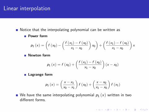
Notice that the interpolating polynomial can be written as

Power form

p1 (x) =

(f (x0)−

(f (x1)− f (x0)

x1 − x0

)x0

)+

(f (x1)− f (x0)

x1 − x0

)x

Newton form

p1 (x) = f (x0) +

(f (x1)− f (x0)

x1 − x0

)(x − x0)

Lagrange form

p1 (x) =

(x − x1x0 − x1

)f (x0) +

(x − x0x1 − x0

)f (x1)

We have the same interpolating polynomial p1 (x) written in twodifferent forms.

Quadratic interpolation

If we assume n = 2 and three data points

(x0, f (x0)) , (x1, f (x1)) , (x2, f (x2))


The interpolation conditions are

f (x0) = p2 (x0) = a0 + a1x0 + a2x20

f (x1) = p2 (x1) = a0 + a1x1 + a2x21

f (x2) = p2 (x2) = a0 + a1x2 + a2x22


In matrix form the interpolation conditions are 1 x0 x201 x1 x211 x2 x22

a0a1a2

=

f (x0)f (x1)f (x2)

or im more compact form

Va = b

Notice that V is a Vandermonde matrix which is ill-conditioned.

The condition number of V is large so it is better to compute the a′sby using another form of writing the interpolating polynomial.


But we can still do it by hand since this is a 3by3 matrix!

Solving the above system yields

a0a1a2

=

x1x2

(x0−x1)(x0−x2)−x0x2

(x0−x1)(x1−x2)x0x1

(x0−x2)(x1−x2)−(x1+x2)

(x0−x1)(x0−x2)x0+x2

(x0−x1)(x1−x2)−(x0+x1)

(x0−x2)(x1−x2)1

(x0−x1)(x0−x2)−1

(x0−x1)(x1−x2)1

(x0−x2)(x1−x2)

f (x0)

f (x1)f (x2)


Or by using the Matlab symbolic toolbox

>> syms a b c

>> A = [1 a a^2; 1 b b^2; 1 c c^2];

>> inv(A)

ans =

[ (b*c)/((a - b)*(a - c)), -(a*c)/((a - b)*(b - c)),

(a*b)/((a - c)*(b - c))]

[ -(b + c)/((a - b)*(a - c)), (a + c)/((a - b)*(b - c)),

-(a + b)/((a - c)*(b - c))]

[ 1/((a - b)*(a - c)), -1/((a - b)*(b - c)), 1/((a - c)*(b

- c))]


Solving the above system yields the coefficients:

a0 =

(x1x2

(x0 − x1) (x0 − x2)

)f (x0) +

(−x0x2

(x0 − x1) (x1 − x2)

)f (x1)

+

(x0x1

(x0 − x2) (x1 − x2)

)f (x2)

a1 =

(− (x1 + x2)

(x0 − x1) (x0 − x2)

)f (x0) +

(x0 + x2

(x0 − x1) (x1 − x2)

)f (x1)

+

(− (x0 + x1)

(x0 − x2) (x1 − x2)

)f (x2)

a2 =

(1

(x0 − x1) (x0 − x2)

)f (x0) +

(−1

(x0 − x1) (x1 − x2)

)f (x1)

+

(1

(x0 − x2) (x1 − x2)

)f (x2)


The approximating second order polynomial in ”power” form is

p2 (x) = a0 + a1x + a2x2

where a0, a1 and a2 are defined above.

Notice that p2 (x) is a linear combination of n + 1 = 3 monomialseach of degree 0, 1, 2.


After ”some” algebra we can write p2 (x) in different forms:

Lagrange form

p2 (x) = f (x0)

((x − x1)

(x0 − x1)

(x − x2)

(x0 − x2)

)+ f (x1)

((x − x0) (x − x2)

(x1 − x0) (x1 − x2)

)+ f (x2)

((x − x0) (x − x1)

(x2 − x0) (x2 − x1)

)The above is a linear combination of n + 1 = 3 polynomials ofdegree n = 2. The coefficients are the interpolated valuesf (x0) , f (x1) and f (x2) .


By doing ”some” algebra we can write p2 (x) in different forms:

Newton form

p2 (x) = f (x0) +

(f (x1)− f (x0)

x1 − x0

)(x − x0)

+

(f (x2)−f (x1)(x2−x1)

)−(f (x1)−f (x0)(x1−x0)

)(x2 − x0)

(x − x0) (x − x1)

The above is a linear combination of n + 1 = 3 polynomials each ofdegree 0, 1, 2. The coefficients are the called divided differences.

Interpolation: The general case

The interpolation conditions when we have n + 1 data points:{(x0, f (x0)) , (x1, f (x1)) , ..., (xn, f (xn))}

f (xi ) = pn (xi ) ∀i : 0, ...n

pn (xi ) written in ”power” form is

pn (xi ) =n

∑j=0

ajxj


The interpolation conditions can be written as

f (xi ) =n

∑j=0

ajxji ∀i : 0, ...n

orf (x0) = a0 + a1x0 + ... + anxn0

f (x1) = a0 + a1x1 + ... + anxn1...

f (xn) = a0 + a1xn + ... + anxnn


In matrix form1 x0 ... xn01 x1 ... xn1... ... ... ...1 xn ... xnn

a0a1...an

=

f (x0)f (x1)

...f (xn)

The matrix to be inverted is a Vandermonde matrix: Also anill-conditioned matrix.


We can also generalize the lagrange form of the interpolatingpolynomial:

pn (x) = f (x0) ln,0 (x) + f (x1) ln,1 (x) + ... + f (xn) ln,n (x)

where{

ln,j (x)}nj=0 are a family of n + 1 polynomials of degree n

given by

ln,j (x) =(x − x0) ...

(x − xj−1

) (x − xj+1

)... (x − xn)(

xj − x0)

...(xj − xj−1

) (xj − xj+1

)...(xj − xn

) ∀0 ≤ j ≤ n

More compactly

pn (x) =n

∑j=0

f(xj)

ln,j (x)


For j = 0

ln,0 (x) =(x − x1) ... (x − xn)

(x0 − x1) ... (x0 − xn)=

n

∏j=0j 6=0

x − xjx0 − xj

For j = 1

ln,1 (x) =(x − x0) (x − x2) ... (x − xn)

(x1 − x0) (x1 − x2) ... (x1 − xn)=

n

∏j=0j 6=1

x − xjx1 − xj

For j = n

ln,n (x) =(x − x0) (x − x2) ... (x − xn−1)

(xn − x0) (xn − x2) ... (xn − xn−1)=

n

∏j=0j 6=2

x − xjx2 − xj


For any ∀0 ≤ j ≤ n

ln,j (x) =n

∏j=0j 6=i

x − xjxi − xj

The lagrange form of the interpolating polynomial is

pn (x) =n

∑j=0

f(xj)

ln,j (x)

with ln,j (x) defined above.

It turns out that computing the lagrange polynomial is more efficientthan solving the vandermonde matrix!


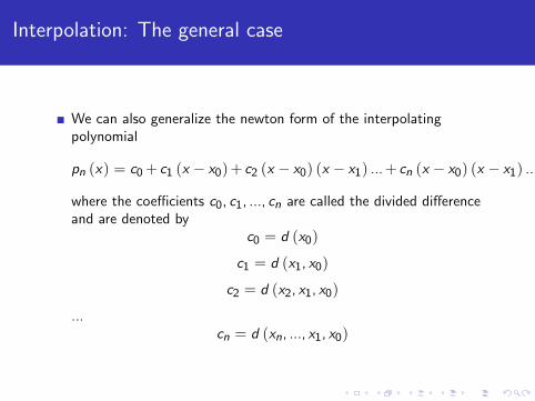
We can also generalize the newton form of the interpolatingpolynomial

pn (x) = c0+ c1 (x − x0)+ c2 (x − x0) (x − x1) ...+ cn (x − x0) (x − x1) ... (x − xn−1)

where the coefficients c0, c1, ..., cn are called the divided differenceand are denoted by

c0 = d (x0)

c1 = d (x1, x0)

c2 = d (x2, x1, x0)

...cn = d (xn, ..., x1, x0)


The divided differences are defined as

d (x0) = f (x0)

d (x1, x0) =f (x1)− f (x0)

x1 − x0

d (x2, x1, x0) =d (x2, x1)− d (x1, x0)

x2 − x0

=

(f (x2)−f (x1)

x2−x1

)−(f (x1)−f (x0)

x1−x2

)x2 − x0


The divided differences are defined as (Cont.)

d (x3, x2, x1, x0) =d (x3, x2, x1)− d (x2, x1, x0)

x3 − x0

=

( (f (x3)−f (x2)

x3−x2

)−(f (x2)−f (x1)

x2−x1

)x3−x2

)−( (

f (x2)−f (x1)x2−x1

)−(f (x1)−f (x0)

x1−x2

)x2−x0

)x3 − x0

d (xn, ..., x1, x0) =d (xn, ..., x1, x0)− d (xn−1, ..., x1, x0)

xn − x0


The generalization of the Newton form of the interpolatingpolynomial is

pn (x) = d (x0) + d (x1, x0) (x − x0) + d (x2, x1, x0) (x − x0) (x − x1) + ...

+ d (xn, ..., x1, x0) (x − x0) (x − x1) ... (x − xn−1)

or

pn (x) = d (x0) +n

∑j=1

d(xj , ..., x1, x0

) j−1

∏k=0

(x − xk )

Interpolation: The interpolation error

Theorem

Let f (x) ∈ Cn+1[a, b]. Let pn (x) a polynomial of degree ≤ n such thatit interpolates f (x) at the n + 1 distinct nodes {x0, x1, ..., xn} . Then∀x ∈ [a, b], there exists a ξn ∈ (a, b) such that

f (x)− pn (x) =1

(n + 1)!f (n+1) (ξn)

n

∏k=0

(x − xk )

Fact

The error term for the nth Taylor approximation around the point x0 is

f (n+1) (ξn)

(n + 1)!(x − x0)

n+1


Notice that applying the supremum norm to the interpolation erroryields

‖f (x)− pn (x)‖∞ ≤1

(n + 1)!

∥∥∥f (n+1) (ξn)∥∥∥

∞

∥∥∥∥∥ n

∏k=0

(x − xk )

∥∥∥∥∥∞

or

maxx∈[a,b]

|f (x)− pn (x)|

≤ 1

(n + 1)!

(max

ξn∈[a,b]

∣∣∣f (n+1) (ξn)∣∣∣)( max

x∈[a,b]

∣∣∣∣∣ n

∏k=0

(x − xk )

∣∣∣∣∣)

The R.H.S is an upper bound for the interpolation error.


We would like to have

limn→∞

{1

(n + 1)!

(max

ξn∈[a,b]

∣∣∣f (n+1) (ξn)∣∣∣)( max

x∈[a,b]

∣∣∣∣∣ n

∏k=0

(x − xk )

∣∣∣∣∣)}

= 0

thuslimn→∞

(f (x)− pn (x)) = 0

But nothing guarantees convergence (neither point or uniformconvergence).


The maximun error depends on the interpolation nodes

{x0, x1, ..., xn} through the term

(maxx∈[a,b]

∣∣∣∣∣ n

∏k=0

(x − xk )

∣∣∣∣∣)

.

Notice that no other term depends on the interpolating nodes oncewe look for the maximum error.

We can choose the nodes in order to minimize the interpolationerror:

min{x0,...,xn}

{max

x∈[a,b]

∣∣∣∣∣ n

∏k=0

(x − xk )

∣∣∣∣∣}

Interpolation: Choosing the nodes

What happens if we work with uniformly spaced nodes?, that is withnodes such that

xi = a +

(i − 1

n− 1

)(b− a) for i : 1, .., n

Recall that:

We want to interpolate a function f (x) : [a, b]→ R

n is the degree of the interpolating polynomial: pn (x)The interpolation conditions are

f (xi ) = pn (xi ) ...for i : 0, .., n

so, if n = 10, we need n+ 1 = 11 data points.


Runge’s example: Let f (x) = 11+x2

defined on the interval [−5, 5].

Find the lagrange polnomial approximation for n = 11.


runge example lagrange interpolation UN.m

Play increasing the degree of interpolation and see that there is noconvergence.

The graph replicates figure 6.6 of Judd’s book.


But we can choose the nodes in order to obtain the smallest value for∥∥∥∥∥ n

∏k=0

(x − xk )

∥∥∥∥∥∞

= maxx∈[a,b]

∣∣∣∣∣ n

∏k=0

(x − xk )

∣∣∣∣∣Chebyshev polynomials one more time: Recall the monicChebyshev polynomial is

T̃j (x) =cos (j arccos x)

2j−1

with x ∈ [−1, 1] and j = 1, 2, ..., n

Then, the zeros of T̃n (x) are given by the soltution to

T̃n (x) = 0

cos (n arccos x) = 0

cos (nθ) = 0

where θ = arccos x . Thus θ ∈ [0, π].


Zeros occur when cos (nθ) = 0, that is

nθ =

(2k − 1

2

)π for k = 1, 2, ..n

Notice that

cos

(2k − 1

2π

)= cos

(kπ − π

2

)= cos (kπ) cos

(π

2

)︸︷︷︸

=0

− sin (kπ)︸︷︷︸=0

sin(π

2

)= 0


The equation T̃n (x) = 0 has n different roots given by

nθ =

(k − 1

2

)π for k = 1, 2, ..n

This means that

For k = 1θ1 =

π

2nFor k = 2

θ2 =

(3

2

)π

n

For k = n

θn =

(2n− 1

2

)π

n


Roots for cos (nθ) where θ ∈ [0, π] :

n = 1 n = 2 n = 3 ... nk = 1 π

2π4

π6

π2n

k = 2 34π 3

6π 32nπ

k = 3 56π 5

2nπ...

k = n(2n−12n

)π


Plooting cos (jθ) for θ ∈ [0, π] and j = 1, 2, ..., n


cheby nodes.m


We want the roots of the monic chebyshev and we have the roots ofthe cosine function:

nθ =

(k − 1

2

)π for k = 1, 2, ..n

but θ = arccos x , thus

arccos x =

(2k − 1

2n

)π for k = 1, 2, ..n

then the roots of the chebyshev polynomials are

xk = cos

((2k − 1

2n

)π

)for k = 1, 2, ..n

Notice that the roots of T̃n (x) are the same as the roots of Tn (x) .


Ploting chebyshev nodes


cheby nodes.m


The following theorem summarizes some characteristics of chebyshevpolynomials

Theorem

The Chebyshev polynomial Tn (x) of degree n ≥ 1 has n zeros in [−1, 1]at

xk = cos

((2k − 1

2n

)π

)for k = 1, 2, ..n

Moreover, Tn (x) assumes its extremum at

x∗k = cos

(kπ

n

)for k = 0, 1, .., n

withTn (x

∗k ) = (−1)k for k = 0, 1, .., n


Corollary

The monic Chebyshev polynomial T̃n (x) has the same zeros andextremum points as Tn (x) but with extremum values given by

T̃n (x∗k ) =

(−1)k

2n−1for k = 0, 1, ..., n


Extrema of Chebyshev polynomials:

Tn (x) = cos (n arccos x)

then

dTn (x)

dx= T ′n (x)

= − sin (n arccos x)

(− n√

1− x2

)=

n sin (n arccos x)√1− x2

Notice that T ′n (x) is a polynomial of degree n− 1 with zeros givenby

T ′n (x) = 0


Excluding the endpoints of the domain, x = −1 or x = 1, then,extremum points occurs when

sin (n arccos x) = 0

or whensin (nθ) = 0

for θ ∈ (0, π). Thus

nθk = kπ for all k = 1, 2, ..., n− 1

Solving for x yields

θ = arccos x =kπ

n

=⇒ x∗k = cos

(kπ

n

)for k = 1, 2, ..., n− 1

Obviusly, extrema also occur at the endpoints of the domain (i.e,x = −1 or x = 1), that is when k = 0 or when k = n.


The extremum values of Tn (x) occurs when

Tn (x∗) = cos (n arccos x∗)

= cos

(n arccos

(cos

(kπ

n

)))= cos

(n

kπ

n

)= cos (kπ)

= (−1)k for k = 0, 1, ..., n

Notice that we are including the endpoints of the domain.

The above result implies

maxx∈[−1,1]

|Tn (x)| = 1


Extrema for monic Chebyshev polynomials are characterized by thesame points since

T̃n (x) =Tn (x)

2n−1

thusT̃ ′n (x

∗k ) = T

′n (x

∗k ) = 0 for k = 0, 1, ..., n

But the extremum values of T̃n (x) are given by

T̃n (x∗k ) =

Tn(x∗k)

2n−1for k = 0, 1, ..., n

=(−1)k

2n−1for k = 0, 1, ..., n

Therefore

maxx∈[−1,1]

∣∣∣T̃n (x)∣∣∣ = 1

2n−1


An important property of monic Chebyshev polynomials is given bythe following theorem

Theorem

If p̃n (x) is a monic polynomial of degree n defined on [−1, 1], then

maxx∈[−1,1]

∣∣∣T̃n (x)∣∣∣ = 1

2n−1≤ max

x∈[−1,1]|p̃n (x)|

for all monic polynomials of degree n.


Recall that we want to choose the interpolation nodes {x0, ..., xn} inorder to solve

min{x0,...,xn}

{max

x∈[a,b]

∣∣∣∣∣ n

∏k=0

(x − xk )

∣∣∣∣∣}

Choosing the interpolation nodes is the same as choosing the zeros

ofn

∏k=0

(x − xk ) .

Notice thatn

∏k=0

(x − xk ) is a monic polynomial of degree n + 1.

Therefore it must be the case that

maxx∈[−1,1]

∣∣∣T̃n+1 (x)∣∣∣ = 1

2n≤ max

x∈[−1,1]

∣∣∣∣∣ n

∏k=0

(x − xk )

∣∣∣∣∣


The smallest value that maxx∈[−1,1]

∣∣∣∣∣ n

∏k=0

(x − xk )

∣∣∣∣∣ can take is 12n .

Therefore

maxx∈[−1,1]

∣∣∣∣∣ n

∏k=0

(x − xk )

∣∣∣∣∣ = 1

2n

= maxx∈[−1,1]

∣∣∣T̃n+1 (x)∣∣∣

which implies thatn

∏k=0

(x − xk ) = T̃n+1 (x)

Therefore the zeros ofn

∏k=0

(x − xk ) must be the zeros of T̃n+1 (x)

which are given by

xk = cos

((2k + 1

2 (n + 1)

)π

)for k = 1, 2, ..n + 1


Since maxx∈[−1,1]

∣∣∣∣∣ n

∏k=0

(x − xk )

∣∣∣∣∣ = 12n then the maximum

interpolation error becomes

maxx∈[a,b]

|f (x)− pn (x)| ≤1

(n + 1)!

(max

ξn∈[a,b]

∣∣∣f (n+1) (ξn)∣∣∣)( max

x∈[a,b]

∣∣∣∣∣ n

∏k=0

(x − xk )

∣∣∣∣∣)

maxx∈[a,b]

|f (x)− pn (x)| ≤1

(n + 1)!

(max

ξn∈[a,b]

∣∣∣f (n+1) (ξn)∣∣∣) ( 1

2n

)Chebyshev nodes eliminate violent oscillations for the error termcompared to uniform spaced nodes.

Interpolation with Chebyshev nodes has better convergenceproperties.

It is possible to show that pn (x)→ f (x) as n→ ∞ uniformly. Thisis not guaranteed under uniform spaced nodes.


Runge’s example with chebyshev nodes

runge example cheby nodes.m


Figure 6.2 of Miranda and Flecker book:

Comparing the interpolation errors of f (x) = exp(−x) defined inx ∈ [−5, 5] with 10-node polynomial approximation

example miranda cheby nodes

Interpolation through regresssion

The interpolation conditions require to have the same number ofdata points (interpolation data) and unknown coefficients in order toproceed.

But we can also have the case, where the data points exceed thenumber of unknow coefficients.

For this case, we can use discrete least squares: Use minterplation points to find n < m coefficients.

The omitted terms are high degree polynomials that may produceundesirable oscillations.The result is a smoother function that approximates the data.


Objective: Construct a degree n polynomial , f̂ (x) , thatapproximates the function f for x ∈ [a, b] using m > n interpolationnodes.

f̂ (x) =n

∑j=0

cjTj (xk )


Algorithm:

Step 1: Compute the m Chebyshev interpolation nodes on[−1, 1]:

zk = cos

((2k − 1

2m

)π

)for k = 1, ..., m

As if we want an m−degree Chebyshev interpolation.

Step 2: Adjust the nodes to the interval [a, b] :

xk = (zk + 1)

(b− a

2

)+ a for k = 1, ..., m

Step 3: Evaluate f at the nodes:

yk = f (xk ) ...for k = 1, ..., m


Algorithm (Cont.):

Step 4: Compute the Chebyshev least squares coefficients

The coefficients that solve the discrete LS problem

minm

∑k=1

[yk −

n

∑j=0

cjTj (zk )

]2are given by

cj =

m

∑k=1

ykTj (zk )

m

∑k=1

(Tj (zk )

)2 for j = 0, 1, ..., n

where zk is the inverse transformation of xk :

zk =2xk − (a+ b)

b− a


Finally, the LS Chebyshev approximating polynomial is given by

f̂ (x) =n

∑j=0

cjTj (z)

where z ∈ [−1, 1] and it is given by

z =2x − (a + b)

b− a

and the cj are estimated using the LS coefficients

cj =

m

∑k=1

ykTj (zk )

m

∑k=1

(Tj (zk )

)2 for j = 0, 1, ..., n

Piecewise linear approximation

If we have interpolation data given by{(x0, f (x0)) , (x1, f (x1)) , ..., (xn, f (xn))}We can divide the interpolation nodes in subintervals of the form

[xi , xi+1] for i = 0, 1, ..., n− 1

Then we can perform linear interpolation in each subinterval:

Interpolation conditions for each subinterval:

f (xi ) = a0 + a1xi

f (xi+1) = a0 + a1xi+1

Piecewise linear approximation

Linear interpolation in each subinterval yields [xi , xi+1]:

The interpolating coefficients:

a0 = f (xi )−(f (xi+1)− f (xi )

xi+1 − xi

)xi

a1 =f (xi+1)− f (xi )

xi+1 − xi

Piecewise linear interpoland:

pi (x) = f (xi ) +

(x − xi

xi+1 − xi

)(f (xi+1)− f (xi ))

Piecewise linear approximationPiecewise polynomialapproximation: Splines

Example: (x0, f (x0)) , (x1, f (x1)) , (x2, f (x2))

Then we have two subintervals

[x0, x1] and .[x1, x2]

The interpolating function is given by:

f̂ (x) =

{f (x0) +(

x−x0x1−x0

)(f (x1)− f (x0)) for x ∈ [x0, x1]

f (x1) +(

x−x1x2−x1

)(f (x2)− f (x1)) for x ∈ [x1, x2]

Piecewise polynomial approximation: Splines

A spline is any smooth function that is piecewise polynomial but alsosmooth where the polynomial pieces connect.

Assume that the interpolation data is given by{(x0, f (x0)) , (x1, f (x1)) , ..., (xm, f (xm))} .

A function s (x) defined on [a, b] is a spline of order n if:

s is Cn−2 on [a, b]s (x) is a polynomial of degree n− 1 on each subinterval [xi , xi+1]for i = 0, 1, ..,m− 1

Notice that an order 2-spline is the piecewise linear interpolantequation.


A cubic spline is a spline of order 4:

s is C2 on [a, b]s (x) is a polynomial of degree n− 1 = 3 on each subinterval[xi , xi+1] for i = 0, 1, ..,m− 1

s (x) = ai + bix + cix2 + dix

3 for x ∈ [xi , xi+1], i = 0, 1, ..,m− 1


Example of cubic spline: Assume that we have the following 3 datapoints: (x0, f (x0)) , (x1, f (x1)) , (x2, f (x2))

There are two subintervals: [x0, x1] and .[x1, x2].

A cubic spline is a function s such that

s is C2 on [a, b]s (x) is a polynomial of degree 3 on each subinterval:

s (x) =

{s0 (x) = a0 + b0x + c0x

2 + d0x3 for x ∈ [x0, x1]

s1 (x) = a1 + b1x + c1x2 + d1x3 for x ∈ [x1, x2]

Notice that in this case we have 8 unknowns:a0, a1, b0, b1, c0, c1, d0, d1


Example (Cont.): We need 8 conditions

Interpolation and continuity at interior nodes conditions

y0 = s0 (x0) = a0 + b0x0 + c0x20 + d0x

30

y1 = s0 (x1) = a0 + b0x1 + c0x21 + d0x

31

y1 = s1 (x1) = a1 + b1x1 + c1x21 + d1x

31

y2 = s1 (x2) = a1 + b1x2 + c1x22 + d1x

32


Example (Cont.): We need 8 conditions

First and second derivatives must agree at the interior nodes

s ′0 (x1) = s ′1 (x1)

b0 + 2c0x1 + 3d0x21 = b1 + 2c1x1 + 3d1x

21

s′′0 (x1) = s

′′1 (x1)

2c0 + 6d0x1 = 2c1 + 6d1x1


Up to know we have 6 conditions, we need two more conditions

3 ways to obtain the additional conditions:

Natural spline: s ′ (x0) = s ′ (x2) = 0Hermite spline: If we have information on the slope of the originalfunction at the end points:

f ′ (x0) = s ′ (x0)

f ′ (x2) = s ′ (x2)

Secant Hermite spline: use the secant to estimate the slope at theend points

s ′ (x0) =s (x1)− s (x0)

x1 − x0

s ′ (x2) =s (x2)− s (x1)

x2 − x1


Generalization of cubic splines:

See Judd’s book!!!

function approximation - ucsc directory of individual web...

Documents