Fully Momentum-Conserving Reduced Deformable Bodies with Collision,Contact, Articulation, and Skinning

Rahul Sheth∗

Stanford UniversityPixar Animation Studios

Wenlong Lu∗

Stanford UniversityYue Yu∗

Stanford UniversityRonald Fedkiw∗

Stanford UniversityIndustrial Light & Magic

Abstract

We propose a novel framework for simulating reduced deformablebodies that fully accounts for linear and angular momentum conser-vation even in the presence of collision, contact, articulation, andother desirable effects. This was motivated by the observation thatthe mere excitation of a single mode in a reduced degree of freedommodel can adversely change the linear and angular momentum. Al-though unexpected changes in linear momentum can be avoidedduring basis construction, adverse changes in angular momentumappear unavoidable, and thus we propose a robust framework thatincludes the ability to compensate for them. Enabled by this abilityto fully account for linear and angular momentum, we introduce animpulse-based formulation that allows us to precisely control thevelocity of any node in spite of the fact that we only have access toa lower-dimensional set of degrees of freedom. This allows us tomodel collision, contact, and articulation in a robust and high visualfidelity manner, especially when compared to penalty-based forcesthat merely aim to coerce local velocities. In addition, we propose anew “deformable bones” framework wherein we leverage standardskinning technology for “bones,” “bone” placement, blending op-erations, etc. even though each of our “deformable bones” is a fullysimulated reduced deformable model.

CR Categories: I.3.7 [Computer Graphics]: Three-DimensionalGraphics and Realism—Animation

Keywords: deformable bodies, elasticity, collisions, skinning,model reduction, subspace

1 Introduction

Simulations of deformable objects are known to be both visuallyinteresting and computationally demanding. One way to lessen thecomputational expense of these simulations is to use a reduced-order (or subspace) model to represent the internal dynamics. Theperformance of such a model depends on the size of the subspace ras well as the basis vectors chosen to represent that space. If n isthe size of the full-order model, optimal performance benefits areachieved when r � n and the simulation takes O (rp) time forsmall values of p.

Basis construction is a difficult problem and many solutionshave been proposed, including modal analysis [Pentland andWilliams 1989], a method to include the derivatives of linearmodes (i.e. modal derivatives) [Idelsohn and Cardona 1985], mass-weighted principal component analysis (PCA) of an existing sim-

∗e-mail: {rbsheth,wenlongl,yuey,fedkiw}@cs.stanford.edu

Figure 1: An articulated reduced deformable body falls down aflight of stairs undergoing collision and self-collision. Even withsimple linear finite elements, the results have high visual fidelitydue to our new “deformable bones” skinning strategy. We stressthat this is a pure simulation of a reduced deformable body, andno misleading techniques such as first simulating a rigid body andthen attaching a deformable skin after the fact were employed.

ulation dataset [Barbic and James 2005], augmentation of the ba-sis with localized displacement vectors [Harmon and Zorin 2013],etc. Regardless of the specific method used, most of the bases con-structed by these methods are linear and can thus be written in a ma-trix form. Our method is compatible with all of the aforementionedapproaches yet does not require mass normalization, but does re-quire full column rank. This keeps the framework as general aspossible and enables an example-based reduced-order scheme thatwe discuss in Section 8.

We use a reduced-order approximation of the displacement ~u =S~q where the columns of S represent particle displacements fromthe rest pose ~x0. Here ~u and ~x0 have dimensions n by 1, S hasn rows and r columns, and the entries of ~u, ~x0 and S are all 3-vectors. Then, particle positions are given by S~q + ~x0, where ~q isa reduced space vector which when set to a basis vector (i.e. ~q ∈{~e1, ~e2, ..., ~er}) results in S~ek + ~x0 reconstructing the kth basisshape. To enable fully unconstrained simulation, we embed thissystem in a rigid frame

~x = R(S~q + ~x0) + ~T (1)

where R is a diagonal matrix of rotations R and ~T is a vector oftranslations ~t. Note that this formulation reduces to a rigid bodywhen there are no internal deformation modes, i.e. when S = 0.This is similar to the method of [Terzopoulos and Witkin 1988]where deformation occurs in a rigid frame.

After assigning each particle a mass (consistent with the require-ment in Section 4), we adjust the rest state ~x0 and each basis shapeS~ek + ~x0 such that their centers of mass are at the origin. This

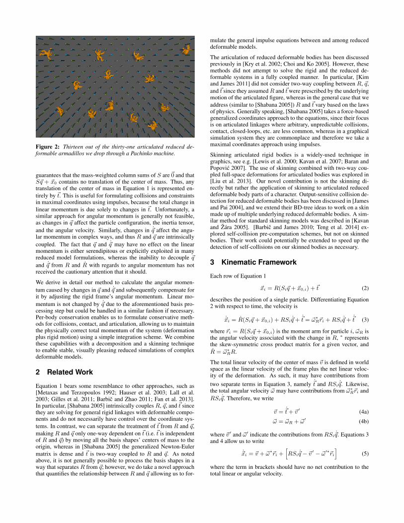
Figure 2: Thirteen out of the thirty-one articulated reduced de-formable armadillos we drop through a Pachinko machine.

guarantees that the mass-weighted column sums of S are~0 and thatS~q + ~x0 contains no translation of the center of mass. Thus, anytranslation of the center of mass in Equation 1 is represented en-tirely by ~t. This is useful for formulating collisions and constraintsin maximal coordinates using impulses, because the total change inlinear momentum is due solely to changes in ~t. Unfortunately, asimilar approach for angular momentum is generally not feasible,as changes in ~q affect the particle configuration, the inertia tensor,and the angular velocity. Similarly, changes in ~q affect the angu-lar momentum in complex ways, and thus R and ~q are intrinsicallycoupled. The fact that ~q and ~q may have no effect on the linearmomentum is either serendipitous or explicitly exploited in manyreduced model formulations, whereas the inability to decouple ~qand ~q from R and R with regards to angular momentum has notreceived the cautionary attention that it should.

We derive in detail our method to calculate the angular momen-tum caused by changes in ~q and ~q and subsequently compensate forit by adjusting the rigid frame’s angular momentum. Linear mo-mentum is not changed by ~q due to the aforementioned basis pro-cessing step but could be handled in a similar fashion if necessary.Per-body conservation enables us to formulate conservative meth-ods for collisions, contact, and articulation, allowing us to maintainthe physically correct total momentum of the system (deformationplus rigid motion) using a simple integration scheme. We combinethese capabilities with a decomposition and a skinning techniqueto enable stable, visually pleasing reduced simulations of complexdeformable models.

2 Related Work

Equation 1 bears some resemblance to other approaches, such as[Metaxas and Terzopoulos 1992; Hauser et al. 2003; Lall et al.2003; Gilles et al. 2011; Barbic and Zhao 2011; Fan et al. 2013].In particular, [Shabana 2005] intrinsically couples R, ~q, and ~t sincethey are solving for general rigid linkages with deformable compo-nents and do not necessarily have control over the coordinate sys-tems. In contrast, we can separate the treatment of ~t from R and ~q,making R and ~q only one-way dependent on ~t (i.e. ~t is independentof R and ~q) by moving all the basis shapes’ centers of mass to theorigin, whereas in [Shabana 2005] the generalized Newton-Eulermatrix is dense and ~t is two-way coupled to R and ~q. As notedabove, it is not generally possible to process the basis shapes in away that separatesR from ~q; however, we do take a novel approachthat quantifies the relationship between R and ~q allowing us to for-

mulate the general impulse equations between and among reduceddeformable models.

The articulation of reduced deformable bodies has been discussedpreviously in [Kry et al. 2002; Choi and Ko 2005]. However, thesemethods did not attempt to solve the rigid and the reduced de-formable systems in a fully coupled manner. In particular, [Kimand James 2011] did not consider two-way coupling between R, ~q,and~t since they assumedR and~twere prescribed by the underlyingmotion of the articulated figure, whereas in the general case that weaddress (similar to [Shabana 2005]) R and ~t vary based on the lawsof physics. Generally speaking, [Shabana 2005] takes a force-basedgeneralized coordinates approach to the equations, since their focusis on articulated linkages where arbitrary, unpredictable collisions,contact, closed-loops, etc. are less common, whereas in a graphicalsimulation system they are commonplace and therefore we take amaximal coordinates approach using impulses.

Skinning articulated rigid bodies is a widely-used technique ingraphics, see e.g. [Lewis et al. 2000; Kavan et al. 2007; Baran andPopovic 2007]. The use of skinning combined with two-way cou-pled full-space deformations for articulated bodies was explored in[Liu et al. 2013]. Our novel contribution is not the skinning di-rectly but rather the application of skinning to articulated reduceddeformable body parts of a character. Output-sensitive collision de-tection for reduced deformable bodies has been discussed in [Jamesand Pai 2004], and we extend their BD-tree ideas to work on a skinmade up of multiple underlying reduced deformable bodies. A sim-ilar method for standard skinning models was described in [Kavanand Zara 2005]. [Barbic and James 2010; Teng et al. 2014] ex-plored self-collision pre-computation schemes, but not on skinnedbodies. Their work could potentially be extended to speed up thedetection of self-collisions on our skinned bodies as necessary.

3 Kinematic Framework

Each row of Equation 1

~xi = R(Si~q + ~x0,i) + ~t (2)

describes the position of a single particle. Differentiating Equation2 with respect to time, the velocity is

~xi = R(Si~q + ~x0,i) +RSi~q + ~t = ~ω∗R~ri +RSi~q + ~t (3)

where ~ri = R(Si~q + ~x0,i) is the moment arm for particle i, ~ωR isthe angular velocity associated with the change in R, ∗ representsthe skew-symmetric cross product matrix for a given vector, andR = ~ω∗RR.

The total linear velocity of the center of mass ~v is defined in worldspace as the linear velocity of the frame plus the net linear veloc-ity of the deformation. As such, it may have contributions fromtwo separate terms in Equation 3, namely ~t and RSi~q. Likewise,the total angular velocity ~ω may have contributions from ~ω∗R~ri andRSi~q. Therefore, we write

~v = ~t+ ~v ′ (4a)

~ω = ~ωR + ~ω′ (4b)

where ~v ′ and ~ω′ indicate the contributions from RSi~q. Equations 3and 4 allow us to write

~xi = ~v + ~ω∗~ri +[RSi~q − ~v ′ − ~ω′∗~ri

](5)

where the term in brackets should have no net contribution to thetotal linear or angular velocity.

Since the term in brackets in Equation 5 should have no net contri-bution to the total linear momentum, i.e. all the linear momentumis contained in ~v, we may write

R

n∑i=1

miSi~q −M~v ′ = ~0 (6)

where M =∑n

i=1mi is the total mass of all n particles of theobject. Since we adjusted our basis so that S would have massweighted column sums of ~0, the first term in Equation 6 is zero andthus ~v ′ = ~0. That is, ~v = ~t and the velocity of the internal modes ~qmakes no contribution to the total linear momentum of the object.

A similar discussion leads ton∑

i=1

mi~r∗i

[RSi~q − ~ω′∗~ri

]= ~0 (7)

which can be re-arranged and solved for ~ω′ to obtain

~ω′ = I−1n∑

i=1

mi~r∗i RSi~q (8)

where I =∑n

i=1mi(~r∗i )T~r ∗i is the inertia tensor. Ideally, one

could remove all internal rotation from the basis so that ~ω′ = 0 and~ω = ~ωR, which is done trivially for rigid bodies. However it is notclear that one can remove this rotation in general, and therefore onemust account for both ~ω′ and ~ωR.

To further elucidate Equation 8, consider the total global angularmomentum of a body

~Lglobal = ~x∗MM~v +

n∑i=1

mi~r∗i ~vi = ~x∗MM~v +

n∑i=1

Ii~ωi (9)

where ~xM is the world space location of the center of mass, ~viis the relative velocity of particle i with respect to the center ofmass velocity ~v, Ii = mi (~r ∗i )T ~r ∗i is particle i’s contribution tothe inertia tensor, and ~ωi = ~r ∗i ~vi/~r

Ti ~ri is the angular velocity of

particle i due to ~vi with respect to the center of mass. The secondequality in Equation 9 is true because ~r ∗i ~vi = ~r ∗i ~ω

∗i ~ri since the

dilational component of ~vi is annihilated by the cross product with~ri leaving only the rotational component. The summation term inEquation 9 is the angular momentum of the body with respect to itscenter of mass, ~Lbody . Thus, one can more rigorously define thetotal angular velocity ~ω for the deforming body as

~ωdef≡ I−1

n∑i=1

Ii~ωi = I−1~Lbody. (10)

Multiplying Equation 4b by I then results in

~Lbody = I~ω = I(~ωR + ~ω′

). (11)

The reduced degrees of freedom ~q make a non-zero contributionto the global angular momentum, which can be accounted for byadding a global rotational velocity ~ω′ that offsets the contributionfrom ~q keeping the total global angular momentum as representedby ~ω constant. We emphasize that the ability to make a correction tothe global angular velocity along the lines of ~ω′ is quite importantfor conserving angular momentum; the fact that our framework inEquation 1 contains the rotation matrixR allows us to readily makethis modification.

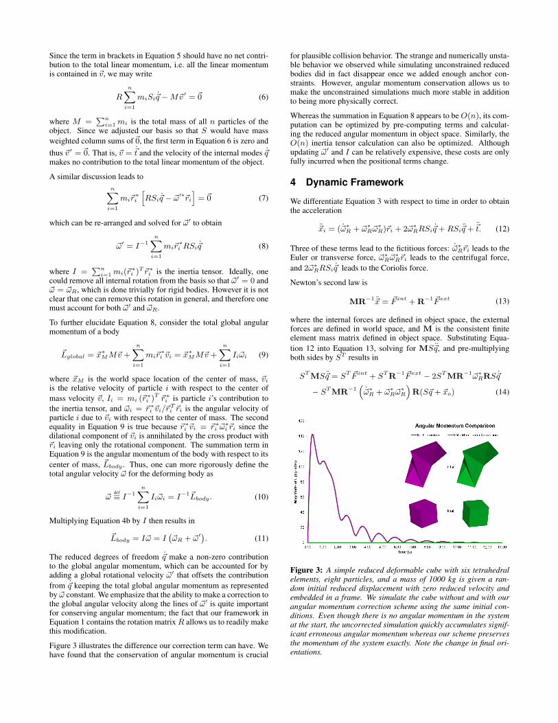
Figure 3 illustrates the difference our correction term can have. Wehave found that the conservation of angular momentum is crucial

for plausible collision behavior. The strange and numerically unsta-ble behavior we observed while simulating unconstrained reducedbodies did in fact disappear once we added enough anchor con-straints. However, angular momentum conservation allows us tomake the unconstrained simulations much more stable in additionto being more physically correct.

Whereas the summation in Equation 8 appears to beO(n), its com-putation can be optimized by pre-computing terms and calculat-ing the reduced angular momentum in object space. Similarly, theO(n) inertia tensor calculation can also be optimized. Althoughupdating ~ω′ and I can be relatively expensive, these costs are onlyfully incurred when the positional terms change.

4 Dynamic Framework

We differentiate Equation 3 with respect to time in order to obtainthe acceleration

~xi = (~ω∗R + ~ω∗R~ω∗R)~ri + 2~ω∗RRSi~q +RSi~q + ~t. (12)

Three of these terms lead to the fictitious forces: ~ω∗R~ri leads to theEuler or transverse force, ~ω∗R~ω

∗R~ri leads to the centrifugal force,

and 2~ω∗RRSi~q leads to the Coriolis force.

Newton’s second law is

MR−1~x = ~F int + R−1 ~F ext (13)

where the internal forces are defined in object space, the externalforces are defined in world space, and M is the consistent finiteelement mass matrix defined in object space. Substituting Equa-tion 12 into Equation 13, solving for MS~q, and pre-multiplyingboth sides by ST results in

STMS~q = ST ~F int + STR−1 ~F ext − 2STMR−1~ω∗RRS~q

− STMR−1(~ω∗R + ~ω∗R~ω

∗R

)R(S~q + ~xo) (14)

Figure 3: A simple reduced deformable cube with six tetrahedralelements, eight particles, and a mass of 1000 kg is given a ran-dom initial reduced displacement with zero reduced velocity andembedded in a frame. We simulate the cube without and with ourangular momentum correction scheme using the same initial con-ditions. Even though there is no angular momentum in the systemat the start, the uncorrected simulation quickly accumulates signif-icant erroneous angular momentum whereas our scheme preservesthe momentum of the system exactly. Note the change in final ori-entations.

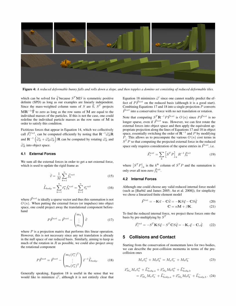
Figure 4: A reduced deformable bunny falls and rolls down a slope, and then topples a domino set consisting of reduced deformable tiles.

which can be solved for ~q because STMS is symmetric positivedefinite (SPD) as long as our examples are linearly independent.Since the mass-weighted column sums of S are ~0, ST projects

MR−1 ~T to zero as long as the row sums of M are equal to theindividual masses of the particles. If this is not the case, one couldredefine the individual particle masses as the row sums of M inorder to satisfy this condition.

Fictitious forces that appear in Equation 14, which we collectivelycall ~F fict

r , can be computed efficiently by noting that R−1~ω∗RR

and R−1(~ω∗R + ~ω∗R~ω

∗R

)R can be computed by rotating ~ω∗R and

~ω∗R into object space.

4.1 External Forces

We sum all the external forces in order to get a net external force,which is used to update the rigid frame as

~v =1

M

n∑k=1

~f extk (15)

~Lbody =

n∑k=1

~r ∗k ~fext

k =

n∑k=1

~τ extk (16)

where ~F ext is ideally a sparse vector and thus this summation is notO (n). When putting the external forces (or impulses) into objectspace, one could project away the translational component before-hand

P ~F ext = ~F ext −

m1

...mn

~v (17)

where P is a projection matrix that performs this linear operation.However, this is not necessary since any net translation is alreadyin the null space of our reduced basis. Similarly, aiming to keep asmuch of the rotation in R as possible, we could also project awaythe rotational component

P ~F ext = ~F ext −

m1(~r ∗1 )T

...mn(~r ∗n)T

I−1 ~Lbody. (18)

Generally speaking, Equation 18 is useful in the sense that wewould like to minimize ~ω′, although it is not entirely clear that

Equation 18 minimizes ~ω′ since one cannot readily predict the ef-fect of P ~F ext on the reduced basis (although it is a good start).Combining Equations 17 and 18 into a single projection P converts~F ext into a conservative force with no net translation or rotation.

Note that computing STR−1P ~F ext is O (n) since P ~F ext is nolonger sparse, even if ~F ext was. However, we can first rotate theexternal forces into object space and then apply the equivalent ap-propriate projection along the lines of Equations 17 and 18 in objectspace, essentially switching the order of R−1 and P by modifyingP . This allows us to precompute the various O (n) cost terms inSTP so that computing the projected external force in the reducedspace only requires consideration of the sparse entries in ~F ext, i.e.

~F extr =

∑k

[STP

]kR−1 ~fext

k (19)

where[STP

]k

is the kth column of STP and the summation isonly over all non-zero ~fext

k .

4.2 Internal Forces

Although one could choose any valid reduced internal force model(such as [Barbic and James 2005; An et al. 2008]), for simplicitywe chose a linearized finite element model

~F int = −K~u−C~u = −KS~q −CS~q (20)C = αM + βK. (21)

To find the reduced internal force, we project these forces onto thebasis by pre-multiplying by ST

~F intr = −STKS~q − STCS~q = −Kr~q −Cr~q. (22)

5 Collisions and Contact

Starting from the conservation of momentum laws for two bodies,we can describe the post-collision momenta in terms of the pre-collision ones

Ma~v+a +Mb~v

+b = Ma~v

−a +Mb~v

−b (23)

~x∗MaMa~v

+a + ~L+

body,a + ~x∗MbMb~v

+b + ~L+

body,b

= ~x∗MaMa~v

−a + ~L−body,a + ~x∗Mb

Mb~v−b + ~L−body,b . (24)

Figure 5: We make the armadillo’s hands and feet static and allowthe rest of the body to deform with articulation constraints. We thenhit the armadillo with various rigid bodies causing deformations inthe armadillo while keeping its hands and feet in place. The handsand feet could also have been moving according to artist-specifiedkinematic paths.

An impulse~jk applied to particle k changes both linear and angularmomentum as follows

Ml~v+l = Ml~v

−l ±~jk (25)

~x∗MlMl~v

+l + ~L+

body,l

= ~x∗MlMl~v

−l + ~L−body,l ± (~xMl + ~rk,l)

∗~jk (26)

for l = a, b. By substituting Equation 25 into Equation 26, we cansimplify Equation 26 to

~L+body,l = ~L−body,l ± ~r

∗k,l~jk. (27)

Using the definition of ~ω in Equation 10, we can rewrite Equa-tion 27 as

~ω+l = ~ω−l ± I

−1l ~r ∗k,l~jk. (28)

Applying only a single impulse via Equation 14 allows us to write(STMS

)∆~q =

[STP

]kR−1~jk with the aid of Equation 19,

which we solve for ∆~q = ~q+ − ~q− to obtain

∆~q =

[(STMS

)−1

STP

]k

R−1~jk = AkR−1~jk (29)

where Ak can be precomputed. Starting from Equation 5 for ~x+k ,

we substitute Equation 25 for ~v+, Equation 28 for ~ω+, and Equa-tion 29 for ~q + to obtain

~x+k = ~v− +~jk/M +

(~ω− + I−1~r ∗k~jk

)∗~rk

+[RSk

(~q − +AkR

−1~jk)−(~ω′− + ∆~ω′

)∗~rk]

(30)

where the unknown change ∆~ω′ equals ~ω′+ − ~ω′−. Rearrangingterms and using Equation 5 to substitute in for ~x−k , we obtain

~x+k = ~x−k +

(1/M − ~r ∗k I−1~r ∗k

)~jk

+RSkAkR−1~jk + ~r ∗k ∆~ω′. (31)

Using the definition of ~ω′ in Equation 8 and the definition of ∆~q inEquation 29 we can write

∆~ω′ = I−1n∑

i=1

mi~r∗i RSiAkR

−1~jk. (32)

Then, we may write

~x+k = ~x−k + (K1 +K2)~jk = ~x−k +K~jk (33a)

K1 = 1/M − ~r ∗k I−1~r ∗k (33b)

K2 = RSkAkR−1 + ~r ∗k I

−1n∑

i=1

mi~r∗i RSiAkR

−1 (33c)

where K1 is the standard rigid body impulse factor and K2 is thenew impulse factor that contains terms for object space deforma-tions. Note that the combined operator is still linear, so we cansolve for impulses quickly just as in the rigid body case. [Hauseret al. 2003] presents an equation similar to Equation 33, althoughtheir equations are incorrect unless ~ω′ = ~0. In our examples, wehave seen that the contribution to angular momentum from ~ω′ isquite significant and cannot be ignored.

5.1 Reduction to Rigid and Deformable Models

We stress that Equation 33 is the most general form of the impulseequation within our framework and is the superset of both the rigidand deformable cases. In the rigid case, S = 0, ~ω′ = ~0, andK2 = 0, leaving only K1 which is the standard impulse factor.In the case of deformable bodies, R is the identity, ~t = ~0, and Sfunctions similar to an identity except that it packs all the scalarcomponents of ~q into a vector of 3-vectors in ~u. In addition, Pis the identity and the net effect of Equation 29 is to divide ~jk bymk. ThenK2 reduces to 1/mk +~r ∗k I

−1~r ∗k . Thus the inertia tensorterms from K1 and K2 cancel, leaving only 1/M + 1/mk. At firstglance, the 1/M seems misplaced, but this is because we have set~t identically zero and have not likewise set ~v ′ = ~v according toEquation 4a. Doing so introduces another term in K2 that cancelsout 1/M leading to the expected result.

5.2 Friction

We model friction after the method in [Guendelman et al. 2003],which first calculates the impulse required to apply static friction,then checks if it is in the friction cone via

∥∥∥~j − (~j · ~n)~n∥∥∥2≤

µ(~j · ~n

)and applies it when within this cone—otherwise apply-

ing kinetic friction. However, we have observed that the globalnature of deformation in reduced deformable models means that~j · ~n can be negative even when ∆~v · ~n = K~j · ~n is posi-tive. This is due to the fact that our angular momentum correc-tion can directly affect the angular velocity of a body in a non-intuitive way and is reminiscent of the Painleve Paradox (see [Kauf-man et al. 2008] for a related discussion on rigid bodies). There-fore, we modified the check from [Guendelman et al. 2003] to be∥∥∥K~j − (K~j · ~n)~n∥∥∥

2≤ µ

(K~j · ~n

). That is, we check the mag-

nitude of the resulting velocity, not the impulse. This situation illus-trates a further problem with penalty forces, where one could applya penalty force to a node in order to make it go in a certain di-rection but the resulting object deformation could instead push thatnode in the opposite direction. Of course, continually applying theforce for a long enough time may eventually coax the entire objectto go in the desired direction, meaning that the penalty force canwork in an unconstrained scenario. However, if the object’s motion

Figure 6: The top figure shows a reduced deformable fish with40 modes, which exhibits well-known linearized rotation artifactsfrom linearized finite elements. The bottom figure shows the fishsegmented into four reduced deformable “bones” (shown in red,yellow, green and blue) with 10 modes each and articulated. Afterskinning the segmented fish along the lines of Figure 7 we obtainthe high visual fidelity shown in Figures 8 and 9.

is constrained in various ways, the penalty force may not properlyinfluence the object to move or deform in any intuitive way what-soever and instead just adds energy to the system.

6 Time Integration

The first step in time integration is to solve Equations 15 and 16in order to update the velocity and total angular momentum of therigid frame. Then, we discretize Equation 14 as

STMS~q n+1 = STMS~q n + ∆t(~F intr + ~F ext

r + ~F fictr

)(34)

where ~F intr and ~F ext

r are defined in Equations 22 and 19 respec-tively. We solve for ~F int

r implicitly and use ~q n+1 = ~q n+∆t~q n+1

to obtain(STMS + ∆tCr + (∆t)2 Kr

)~q n+1

= STMS~q n −∆tKr~qn + ∆t

(~F extr + ~F fict

r

). (35)

Once ~vn+1, ~Ln+1body , and ~q n+1 have been updated, we calculate

~ω′n+1 using Equation 8 and ~ωn+1R using Equation 11. We can then

proceed to update the position terms as normal

~t n+1 = ~t n + ∆t~vn+1 (36)

Qn+1 = Q(∆t~ωn+1

R

)Qn (37)

~q n+1 = ~q n + ∆t~q n+1 (38)

where Q is a quaternion, Equation 37 represents the standardquaternion update rule, and Rn+1 is retrieved from Qn+1. Finally,we update the inertia tensor to In+1 and re-compute both ~ω′n+1

and ~ωn+1R . To handle collisions and contact, we use the scheme

from [Guendelman et al. 2003] in conjunction with our new equa-tions.

7 Articulation

We follow [Weinstein et al. 2006] for articulating reduced de-formable bodies using both pre-stabilization and post-stabilization.For simplicity, we will only consider point joints, but note that thesame ideas can be extended to other types of joints. For the sake

of exposition, assume that we are merely constraining particle i onbody a to particle k on body b, noting that we could constrain arbi-trary points using barycentric weights (similar consideration appliesto collisions in Section 5). Post-stabilization is rather straightfor-ward. We simply apply the impulse that results from equating ~x+

i

and ~x+k using Equation 33a.

During pre-stabilization, the goal is to combat positional drift andmake the positions of the two particles identical using

Ra

(S ai ~qa + ~xa

0,i

)+ ~ta = Rb

(S bk~qb + ~xb

0,k

)+ ~tb (39)

at time n + 1. Since all the terms in Equation 39 are evaluatedat time n + 1, we can substitute the right hand sides of Equa-tions 36, 37, and 38 to obtain

Q(

∆t~ωn+1Ra

)Qn

a

[S ai

(~q na +∆t~q n+1

a

)+~xa

0,i

]+~t n

a +∆t~vn+1a =

Q(

∆t~ωn+1Rb

)Qn

b

[S bk

(~q nb +∆t~q n+1

b

)+~xb

0,k

]+~t n

b +∆t~vn+1b . (40)

We can then define the objective function that we want to make zerovia impulses applied to the time n+ 1 velocities as

~f(~j)

= ~t na + ∆t

(~vn+1a +~j/Ma

)+ Q

(∆t(~ωn+1Ra

+(Ina)−1(

~r ∗~j −∆~ω′na)))

Qna[

S ai

(~q na + ∆t

(~q n+1a +An

a,i (Rna )−1~j

))+ ~xa

0,i

]− ~t n

b −∆t(~vn+1b −~j/Mb

)− Q

(∆t(~ωn+1Rb

+(Inb)−1(

~r ∗~j −∆~ω′nb)))

Qnb[

S bk

(~q nb + ∆t

(~q n+1b −An

b,k (Rnb )−1~j

))+ ~xb

0,k

](41)

where ~r is defined as the world space midpoint between the twotime n positions and ~ω′ is defined using the time n quantities inEquation 32. To solve this equation we use Newton iteration, andthe derivation of ∂ ~f/∂~j needed for the solve follows along the linesof that provided in [Weinstein et al. 2006].

The ability to articulate reduced deformable bodies directly allowsus to segment (or decompose) a simulation mesh into differentpieces and connect them using joints. However, since the bod-ies can deform but cannot deform arbitrarily, there is no guarantee

Figure 7: Naıvely articulating together two reduced deformablerods (top) produces erroneous collision with the ground. Treatingthe two bodies as “bones” of a single deformable body and skin-ning them produces improved results (bottom left). Note that onlythe skin collides, and the simulated bodies do not interact with theenvironment (bottom right).

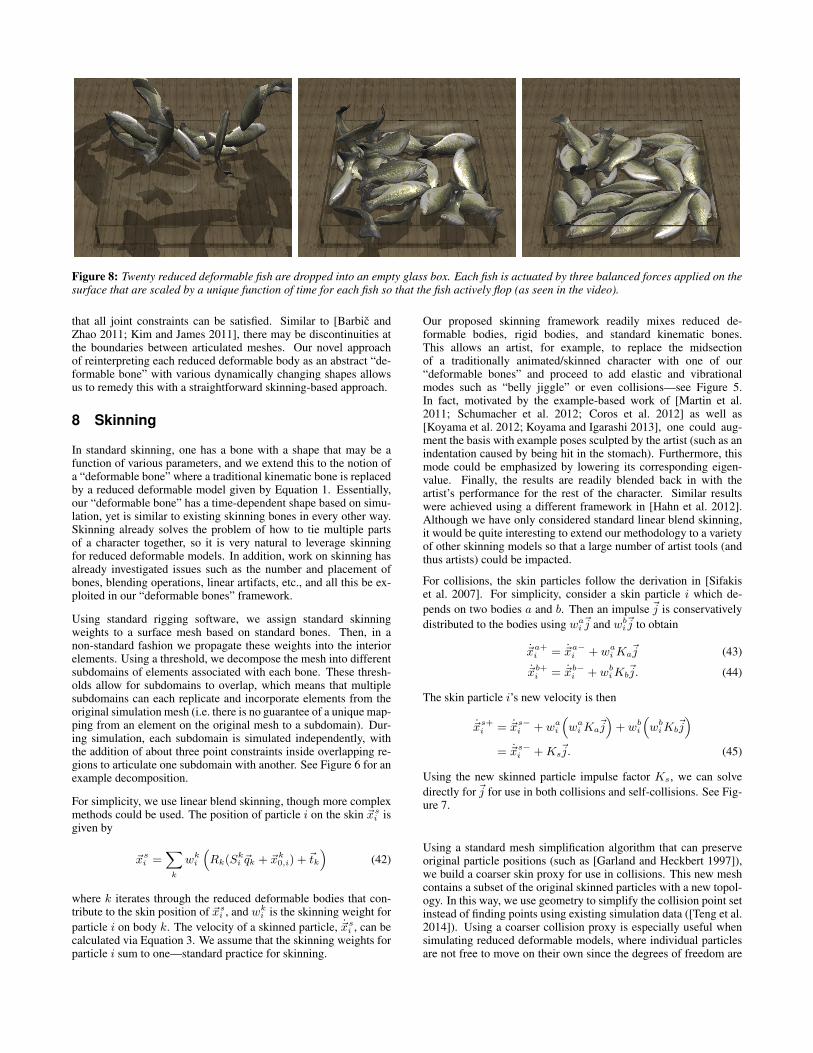
Figure 8: Twenty reduced deformable fish are dropped into an empty glass box. Each fish is actuated by three balanced forces applied on thesurface that are scaled by a unique function of time for each fish so that the fish actively flop (as seen in the video).

that all joint constraints can be satisfied. Similar to [Barbic andZhao 2011; Kim and James 2011], there may be discontinuities atthe boundaries between articulated meshes. Our novel approachof reinterpreting each reduced deformable body as an abstract “de-formable bone” with various dynamically changing shapes allowsus to remedy this with a straightforward skinning-based approach.

8 Skinning

In standard skinning, one has a bone with a shape that may be afunction of various parameters, and we extend this to the notion ofa “deformable bone” where a traditional kinematic bone is replacedby a reduced deformable model given by Equation 1. Essentially,our “deformable bone” has a time-dependent shape based on simu-lation, yet is similar to existing skinning bones in every other way.Skinning already solves the problem of how to tie multiple partsof a character together, so it is very natural to leverage skinningfor reduced deformable models. In addition, work on skinning hasalready investigated issues such as the number and placement ofbones, blending operations, linear artifacts, etc., and all this be ex-ploited in our “deformable bones” framework.

Using standard rigging software, we assign standard skinningweights to a surface mesh based on standard bones. Then, in anon-standard fashion we propagate these weights into the interiorelements. Using a threshold, we decompose the mesh into differentsubdomains of elements associated with each bone. These thresh-olds allow for subdomains to overlap, which means that multiplesubdomains can each replicate and incorporate elements from theoriginal simulation mesh (i.e. there is no guarantee of a unique map-ping from an element on the original mesh to a subdomain). Dur-ing simulation, each subdomain is simulated independently, withthe addition of about three point constraints inside overlapping re-gions to articulate one subdomain with another. See Figure 6 for anexample decomposition.

For simplicity, we use linear blend skinning, though more complexmethods could be used. The position of particle i on the skin ~xs

i isgiven by

~xsi =

∑k

wki

(Rk(Sk

i ~qk + ~xk0,i) + ~tk

)(42)

where k iterates through the reduced deformable bodies that con-tribute to the skin position of ~xs

i , and wki is the skinning weight for

particle i on body k. The velocity of a skinned particle, ~xsi , can be

calculated via Equation 3. We assume that the skinning weights forparticle i sum to one—standard practice for skinning.

Our proposed skinning framework readily mixes reduced de-formable bodies, rigid bodies, and standard kinematic bones.This allows an artist, for example, to replace the midsectionof a traditionally animated/skinned character with one of our“deformable bones” and proceed to add elastic and vibrationalmodes such as “belly jiggle” or even collisions—see Figure 5.In fact, motivated by the example-based work of [Martin et al.2011; Schumacher et al. 2012; Coros et al. 2012] as well as[Koyama et al. 2012; Koyama and Igarashi 2013], one could aug-ment the basis with example poses sculpted by the artist (such as anindentation caused by being hit in the stomach). Furthermore, thismode could be emphasized by lowering its corresponding eigen-value. Finally, the results are readily blended back in with theartist’s performance for the rest of the character. Similar resultswere achieved using a different framework in [Hahn et al. 2012].Although we have only considered standard linear blend skinning,it would be quite interesting to extend our methodology to a varietyof other skinning models so that a large number of artist tools (andthus artists) could be impacted.

For collisions, the skin particles follow the derivation in [Sifakiset al. 2007]. For simplicity, consider a skin particle i which de-pends on two bodies a and b. Then an impulse ~j is conservativelydistributed to the bodies using wa

i~j and wb

i~j to obtain

~xa+i = ~xa−

i + waiKa

~j (43)

~xb+i = ~xb−

i + wbiKb

~j. (44)

The skin particle i’s new velocity is then

~xs+i = ~xs−

i + wai

(wa

iKa~j)

+ wbi

(wb

iKb~j)

= ~xs−i +Ks

~j. (45)

Using the new skinned particle impulse factor Ks, we can solvedirectly for~j for use in both collisions and self-collisions. See Fig-ure 7.

Using a standard mesh simplification algorithm that can preserveoriginal particle positions (such as [Garland and Heckbert 1997]),we build a coarser skin proxy for use in collisions. This new meshcontains a subset of the original skinned particles with a new topol-ogy. In this way, we use geometry to simplify the collision point setinstead of finding points using existing simulation data ([Teng et al.2014]). Using a coarser collision proxy is especially useful whensimulating reduced deformable models, where individual particlesare not free to move on their own since the degrees of freedom are

Figure 9: Twenty-four reduced deformable fish and twelve rigid seashells are dropped onto a slightly slippery floor. After the pile settles,a reduced deformable octopus (skinned from 50 “bones”) drops on top of the fish and seashells, eventually settling with its tentacles beingnudged by the flopping fish tails.

basis shapes. In addition to our collision proxies, we build a BD-tree (see [James and Pai 2004]) on the skin for further accelerations.Although skinned bodies have no intrinsic reduced degrees of free-dom, we would like to express sphere radii in terms of ~qk for each“bone” k for efficiency. Thus our radius bound of each skin sphereis defined as the maximum of its (maximum contained skinningweight-scaled) “bone” radii over all “bones.” This bound is poten-tially looser than that in [James and Pai 2004]. The center updatescan be losslessly accelerated by precomputing for each body k askinning weight average of rows of Sk, ~x0,k, and ~1k correspondingto each sphere’s contained particles.

9 Results and Discussion

We provide several examples to illustrate the power of our method,noting that each example uses linear finite elements (i.e. linearelasticity and linear shape functions) with r ≤ 10 unconstrainedeigenmodes per reduced body unless otherwise specified. Modalanalysis was performed on each reduced body individually; pre-computation times and other mesh-specific details can be found inTable 1. Skeletons were created by first manually placing standardbones in the rest structures of each mesh and obtaining standard lin-ear skinning weights using Pinocchio ([Baran and Popovic 2007]).Segmentation into “deformable bones” was then done by mapping

LinearFEM

BasisGen.

BD-Tree Other # of

Bones# of

ParticlesBunny 0.73 1.93 0.54 0.22 13 7kDomino 0.0081 0.0151 0.0016 0.0035 1 2.7kArmadillo 7.60 45.26 6.20 2.02 21 74kArmadillo(Coarse) 1.14 2.63 1.76 0.39 21 19k

Fish 0.66 1.91 0.47 0.18 4 10kOctopus 21.01 320.99 25.76 6.00 50 244k

Table 1: Pre-computation times (in seconds) and complexity detailsfor all of our example meshes.

the skinning weights from the surface onto the tetrahedral volume,thresholding the weights to create a new tetrahedral volume for eachsegment, and subsequently re-normalizing the weights over the en-tire mesh. Rigid joints were created by automatically laying outthree point joints in a cross section of the overlapping joint region,varying the distance among the three point joints to control rigidityof the connected “deformable bones.”

We focused on the algorithmic portions of our implementation andas such there is much room for optimization to achieve better per-formance, including parallelization. The timing information in Ta-ble 2 hints at the main bottleneck in our simulations, which is the re-duced deformable-reduced deformable collision (and self-collision)step. This aspect of the system could be optimized by implement-ing or designing alternative acceleration structures for our skinnedreduced deformable bodies, perhaps even using a standard kd-treeinstead of a BD-tree. The costs of our inertia tensor update and an-gular momentum correction are negligible compared to the cost ofcollisions, but they could also be optimized similar to how [An et al.2008] reduced the cost of [Barbic and James 2005]. One could alsoattempt less frequent updates of the inertia tensor, ignoring ficti-tious forces, and so on to increase speed at the expense of accuracy,but doing so may introduce instabilities into the system. Our codecurrently allows us to run a skinned armadillo with 30k triangles,19k particles, 21 member “bones,” and 87 point joints with a colli-sion proxy in the Pachinko scenario at the interactive rate of about7fps on a single core of an Intel Xeon X5680 CPU.

Although we have used linear finite elements to simplify our discus-sion, our method can handle non-linear materials as well via [Barbicand James 2005]. Our derivations assume a linear basis (i.e. ~u =S~q), so we would require modal derivatives in the basis to reason-ably handle non-linear materials. One could extend the ideas in thispaper to even more complex subspaces, including those with mul-tiple linear bases. We note that it is straightforward to apply ourskinning framework to standard finite element models as well—forexample one could use a very low degree of freedom linear fullspace finite element model attached to a rigid frame via Equation 1for each ”deformable bone” (or even a very coarse nonlinear finite

# ofFrames

AverageSec/Frame

# ofBones

# of Points ofArticulation

# ofParticles

# of SurfaceParticles

# of CollisionProxy Surface

Particles

Self-Collision

Reduced-ReducedCollision

Bunny and 10 Dominoes 600 35.4 23 64 10k 6k - on onArmadillo and Stairs 400 32.4 21 83 74k 36k - on onArmadillo with Projectiles 500 4.2 21 83 74k 36k - off offArmadillos in a PachinkoMachine (Each Armadillo) 650 0.15 21 87 19k 15k 1536 off off

20 Fish in a Box 480 122.4 80 300 200k 116k 5600 off on20 Fish in a Box 480 13.38 80 300 200k 116k 5600 off off24 Fish and 12 Shells 480 81.6 96 360 240k 139k 6720 off onFish, Shells, and an Octopus 204 344.4 146 591 484k 240k 11762 on on

Table 2: Timing and mesh sizes for all of our examples, which were run using a single core of an Intel Xeon X5680 CPU. For the Pachinkoexample, we set collision, contact, and poststabilization iterations to 1 while setting the iterative articulation tolerance to 0.1. We set collision,contact, and poststabilization iterations to 5 and our iterative articulation tolerance to 1e-7 for all other examples.

element model). A better friction model than the one we chose touse could also be investigated in future work.

10 Conclusion

We have presented a general framework for simulating reduceddeformable bodies (each may specialize to be rigid or fully de-formable) that conserves linear and angular momentum by compen-sating for the often overlooked change in angular momentum due tochanges in the reduced degrees of freedom. Enforcing momentumconservation allows us to achieve plausible and stable simulationsof unconstrained bodies. We have developed a scheme for impulse-based control of individual particle velocities to achieve physicallyaccurate collisions, contact, and point position articulation. Ourskinning of reduced deformable “bones,” when combined with ar-ticulation, achieves domain decomposition and produces detailedand directable local deformations.

11 Acknowledgements

R.S. thanks Tony DeRose, Mark Meyer, and Forrester Cole at PixarAnimation Studios for relevant and insightful discussions. The au-thors also thank Like Gobeawan and Zahid Hossain for their help.R.S. was supported in part by the Department of Energy Office ofScience Graduate Fellowship Program (DOE SCGF), made pos-sible in part by the American Recovery and Reinvestment Act of2009 and administered by ORISE-ORAU under contract no. DE-AC05-06OR23100. Y.Y. was supported by a Stanford GraduateFellowship. This research was supported in part by ONR N00014-13-1-0346, ONR N00014-11-1-0707, ARL AHPCRC W911NF-07-0027, and the Intel Science and Technology Center for VisualComputing. Computing resources were provided in part by ONRN00014-05-1-0479.

References

AN, S. S., KIM, T., AND JAMES, D. L. 2008. Optimizing cuba-ture for efficient integration of subspace deformations. In ACMSIGGRAPH Asia 2008 Papers, ACM, New York, NY, USA, SIG-GRAPH Asia ’08, 165:1–165:10.

BARAN, I., AND POPOVIC, J. 2007. Automatic rigging and ani-mation of 3d characters. ACM Trans. Graph. 26, 3.

BARBIC, J., AND JAMES, D. 2005. Real-time subspace integrationof St. Venant-Kirchhoff deformable models. ACM Trans. Graph.(SIGGRAPH Proc.) 24, 3, 982–990.

BARBIC, J., AND JAMES, D. 2010. Subspace self-collision culling.In Proc. of ACM SIGGRAPH 2010, 81:1–81:9.

BARBIC, J., AND ZHAO, Y. 2011. Real-time large-deformationsubstructuring. ACM Trans. on Graphics (SIGGRAPH 2011) 30,4, 91:1–91:7.

CHOI, M. G., AND KO, H.-S. 2005. Modal warping: Real-time simulation of large rotational deformation and manipula-tion. IEEE Trans. Viz. Comput. Graph. 11, 91–101.

COROS, S., MARTIN, S., THOMASZEWSKI, B., SCHUMACHER,C., SUMNER, R., AND GROSS, M. 2012. Deformable objectsalive! ACM Trans. Graph. 31, 4 (July), 69:1–69:9.

FAN, Y., LITVEN, J., LEVIN, D. I. W., AND PAI, D. K. 2013.Eulerian-on-lagrangian simulation. ACM Trans. Graph. 32, 3(July), 22:1–22:9.

GARLAND, M., AND HECKBERT, P. S. 1997. Surface simpli-fication using quadric error metrics. In Proceedings of the 24thAnnual Conference on Computer Graphics and Interactive Tech-niques, ACM Press/Addison-Wesley Publishing Co., New York,NY, USA, SIGGRAPH ’97, 209–216.

GILLES, B., BOUSQUET, G., FAURE, F., AND PAI, D. K. 2011.Frame-based elastic models. ACM Trans. Graph. 30, 2 (Apr.),15:1–15:12.

GUENDELMAN, E., BRIDSON, R., AND FEDKIW, R. 2003. Non-convex rigid bodies with stacking. ACM Trans. Graph. 22, 3,871–878.

HAHN, F., MARTIN, S., THOMASZEWSKI, B., SUMNER, R.,COROS, S., AND GROSS, M. 2012. Rig-space physics. ACMTrans. Graph. 31, 4 (July), 72:1–72:8.

HARMON, D., AND ZORIN, D. 2013. Subspace integration withlocal deformations. ACM Trans. Graph. 32, 4 (July), 107:1–107:10.

HAUSER, K. K., SHEN, C., AND O’BRIEN, J. F. 2003. Interactivedeformation using modal analysis with constraints. In Graph-ics Interface, A K Peters, CIPS, Canadian Human-ComputerCommnication Society, 247–256. ISBN 1-56881-207-8, ISSN0713-5424.

IDELSOHN, S. R., AND CARDONA, A. 1985. A reduction methodfor nonlinear structural dynamic analysis. Computer Methods inApplied Mechanics and Engineering 49, 3, 253 – 279.

JAMES, D., AND PAI, D. 2004. Bd-tree: Output sensitive collisiondetection for reduced deformable models. ACM Trans. Graph.(SIGGRAPH Proc.) 23, 393–398.

KAUFMAN, D., SUEDA, S., JAMES, D., AND PAI, D. 2008. Stag-gered projections for frictional contact in multibody systems.ACM Transactions on Graphics (SIGGRAPH Asia 2008) 27, 5,164:1–164:11.

KAVAN, L., AND ZARA, J. 2005. Fast collision detection forskeletally deformable models. Computer Graphics Forum 24, 3,363–372.

KAVAN, L., COLLINS, S., ZARA, J., AND O’SULLIVAN, C. 2007.Skinning with dual quaternions. In Proceedings of the 2007Symposium on Interactive 3D Graphics and Games, ACM, NewYork, NY, USA, I3D ’07, 39–46.

KIM, T., AND JAMES, D. L. 2011. Physics-based character skin-ning using multi-domain subspace deformations. In Proceed-ings of the 2011 ACM SIGGRAPH/Eurographics Symposium onComputer Animation, ACM, New York, NY, USA, SCA ’11, 63–72.

KOYAMA, Y., AND IGARASHI, T. 2013. View-dependent controlof elastic rod simulation for 3d character animation. In Sympo-sium on Computer Animation, ACM, J. Chai, Y. Yu, T. Kim, andR. W. Sumner, Eds., 73–78.

KOYAMA, Y., TAKAYAMA, K., UMETANI, N., AND IGARASHI,T. 2012. Real-time example-based elastic deformation. In Pro-ceedings of the ACM SIGGRAPH/Eurographics Symposium onComputer Animation, Eurographics Association, Aire-la-Ville,Switzerland, Switzerland, SCA ’12, 19–24.

KRY, P., JAMES, D., AND PAI, D. 2002. Eigenskin: real time largedeformation character skinning in hardware. In Proc. of the ACMSIGGRAPH Symp. on Comput. Anim., ACM Press, 153–159.

LALL, S., KRYSL, P., AND MARSDEN, J. E. 2003. Structure-preserving model reduction for mechanical systems. Physica D:Nonlinear Phenomena 184, 1, 304–318.

LEWIS, J., CORDNER, M., AND FONG, N. 2000. Pose spacedeformations: A unified approach to shape interpolation a ndskeleton-driven deformation. Comput. Graph. (SIGGRAPHProc.), 165–172.

LIU, L., YIN, K., WANG, B., AND GUO, B. 2013. Simulationand control of skeleton-driven soft body characters. ACM Trans.Graph. 32, 6, 215:1–215:8.

MARTIN, S., THOMASZEWSKI, B., GRINSPUN, E., AND GROSS,M. 2011. Example-based elastic materials. In ACM SIG-GRAPH 2011 papers, ACM, New York, NY, USA, SIGGRAPH’11, 72:1–72:8.

METAXAS, D., AND TERZOPOULOS, D. 1992. Dynamic defor-mation of solid primitives with constraints. In Proceedings ofthe 19th annual conference on Computer graphics and interac-tive techniques, ACM, New York, NY, USA, SIGGRAPH ’92,309–312.

PENTLAND, A., AND WILLIAMS, J. 1989. Good vibrations:modal dynamics for graphics and animation. Comput. Graph.(Proc. SIGGRAPH 89) 23, 3, 215–222.

SCHUMACHER, C., THOMASZEWSKI, B., COROS, S., MARTIN,S., SUMNER, R., AND GROSS, M. 2012. Efficient simulationof example-based materials. In Proceedings of the ACM SIG-GRAPH/Eurographics Symposium on Computer Animation, Eu-

rographics Association, Aire-la-Ville, Switzerland, Switzerland,SCA ’12, 1–8.

SHABANA, A. 2005. Dynamics of Multibody Systems. CambridgeUniversity Press.

SIFAKIS, E., SHINAR, T., IRVING, G., AND FEDKIW, R. 2007.Hybrid simulation of deformable solids. In Proc. of ACM SIG-GRAPH/Eurographics Symp. on Comput. Anim., 81–90.

TENG, Y., OTADUY, M. A., AND KIM, T. 2014. Simulating ar-ticulated subspace self-contact. ACM Trans. Graph. 33, 4 (July),106:1–106:9.

TERZOPOULOS, D., AND WITKIN, A. 1988. Physically basedmodels with rigid and deformable components. In Graph. Inter-face, 146–154.

WEINSTEIN, R., TERAN, J., AND FEDKIW, R. 2006. Dynamicsimulation of articulated rigid bodies with contact and collision.IEEE TVCG 12, 3, 365–374.