Full Waveform Inversion (FWI) ( )with wave-equation migration

(WEM) and well control(WEM) and well controlGary Margravey gRob FergusonChad Hogang

Banff, 3 Dec. 2010

OutlineOutline

The FWI cycleThe FWI cycleThe fundamental theorem of FWI

Understanding the theoremUnderstanding the theoremWhat kind of migration?Calibrating the migrationCalibrating the migration

A numerical experiment with MarmousiConclusionsConclusions

Initial impressions of FWIInitial impressions of FWI

??

Second impression of FWISecond impression of FWI

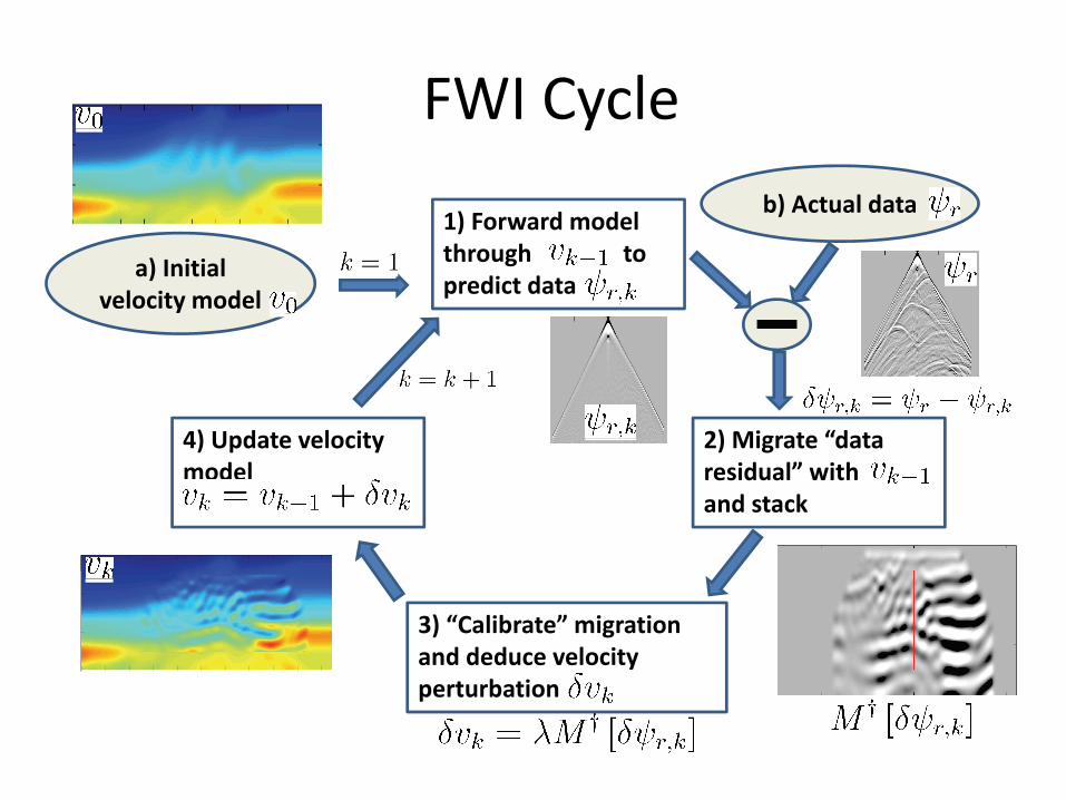
FWI CycleFWI Cycle

1) Forward modelb) Actual data

1) Forward model through to predict data

a) Initial velocity model

2) Migrate “data 4) Update velocity

residual” with and stack

model

3) “Calibrate” migration and deduce velocity perturbationperturbation

Fundamental Theorem of FWIFundamental Theorem of FWITheorem (Tarantola, Lailly): Given real acoustic data and

i t l it d l th li i d l itan approximate velocity model, then a linearized velocity model update, , is given by

A prestack migrationa scalar to be determined (“step length”)

monochromatic, forward propagatedmonochromatic, forward propagated (downward continued), shot model

monochromatic, reverse propagatedmonochromatic, reverse propagated (downward continued), data residual

Understanding the FTFWIUnderstanding the FTFWIInterpretation: A prestack migration of the data residual is

ti l t th d i d d t t th l it d lproportional to the desired update to the velocity model.

This is because the gradient of the data misfit function can be shown to be a type of prestack migration.

A l ti i i diti i t ll dA cross correlation imaging condition arises naturally and there is a frequency squared factor. In the time domain this is a type of reverse –time migration (RTM).

Frequency domain TIme domainFrequency domain TIme domain

Understanding the FTFWIUnderstanding the FTFWIFrequency dependence of :

FTFWI th t th l t i k• FTFWI assumes that the source wavelet is known.• An unknown wavelet is equivalent to a complex-valued (i.e. amplitude and phase), frequency-dependent scalar.

So we write

where the factor has been absorbed into

What kind of migration?What kind of migration?• The direct interpretation of the FTFWI requires a prestackreverse-time migration (RTM) using time-differentiatedreverse time migration (RTM) using time differentiated wavefields.• However, experience suggests that all depth migrations can produce comparable resultscan produce comparable results.•With allowed to be complex and frequency-dependent, there seems no reason that a depth-stepping wave-equation migration (WEM) should not be used.

where is a generalized migration operator and we expect that depends on both the source wavelet and the type of migration.

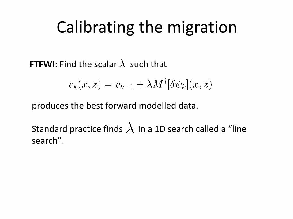
Calibrating the migrationCalibrating the migration

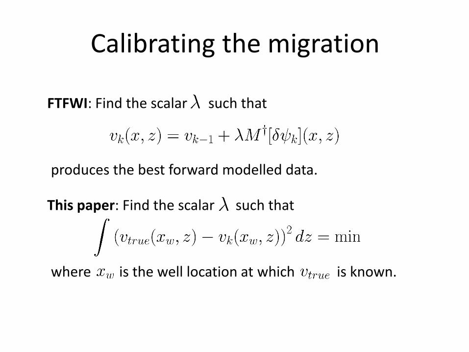
FTFWI Fi d th l h th tFTFWI: Find the scalar such that

produces the best forward modelled data.

Standard practice finds in a 1D search called a “line search”.

Calibrating the migrationCalibrating the migrationThis paper: Find the scalar such that

Defining the velocity residual

where is the well location at which is known.

Defining the velocity residual

So we will match the migrated data residual to the velocity residual at the well. This is a process very similar to standard impedance inversionimpedance inversion.

Calibrating the migrationCalibrating the migrationOur explicit calibration procedure is:

1. Convolve the migrated stack with a Gaussian smoother2. Determine the best (least squares) scalar to match the

smoothed migrated trace at the well to the residualsmoothed migrated trace at the well to the residual velocity at the well.

3. Determine the best (least squares) constant-phase rotation t t h th l d th d i t d t t thto match the scaled, smoothed, migrated trace to the residual velocity at the well.

4. Apply the amplitude scalar and phase rotation to the entire smoothed stack to estimate .

Many other, more sophisticated calibration methods are possible.

Numerical ExperimentNumerical ExperimentUsing data created from the Marmousi model, we implemented the four steps of FWI as:implemented the four steps of FWI as:

1. Modelling using acoustic finite difference tools in l bMatlab.

2. Migration of data residual using PSPI in Matlab.3. Calibration by matching to data residual to velocity y g y

residual at well using least-squares amplitude and constant-phase rotations.

4 Update using addition4. Update using addition.

Marmousi Modelwith shots (red) receivers (white) and well (black)with shots (red), receivers (white), and well (black)

40 h li d f ff 200040 shots, split spread, far offset 2000 m.

ModellingSpectrum of source wavelet

(5 Hz dominant)Spectrum of modelled

datadata

a) b)

Sample ShotsSample Shots0

Shot 1 Shot 20 Shot 40

1.0

Seco

nds

2.0

S

6000 80004000Meters

8000 100006000Meters

4000 60002000Meters Meters MetersMeters

Initial Velocity ModelGaussian smoother 580m width

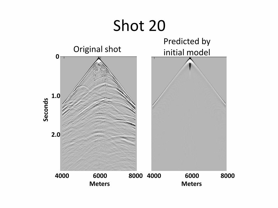
Shot 20Shot 20Original shot

0

Predicted by initial model

1.0

Seco

nds

2.0

S

4000 6000 8000 4000 6000 8000Meters Meters

First Migration (0-5 Hz) with and without modellingn

Migration of full data Migration of data residual

nvol

utio

n g

cond

ition

Deco

nIm

agin

gat

ion

ditio

nro

ss C

orre

lam

agin

g co

ndCr Im

Calibration at the wellFirst iteration 0 5 HzFirst iteration 0-5 Hz.

Migration Before update After update

Extent of well.

Blue is the exact velocity at the well. Red is the migration velocity.

0After 1 Iteration 0-5 Hz

b)

0

1000

met

ers 5000 m/s

4000 m/s

05000 m/s

2000m 3000 m/s

2000 m/s

b)1000

2000met

ers 5000 m/s

4000 m/s

3000 m/s2000 3000 m/s

2000 m/s0

s 5000 m/s

b)1000

2000met

ers

4000 m/s

3000 m/s

2000 4000 6000 8000meters

2000 m/s

Frequency IterationIteration 1, 1-4 Hz Iteration 2, 5-6 Hz Iteration 3, 5-10 Hz

Iteration 5, 10-20 Hz Iteration 11, 25-35 Hz Iteration 22, 55-60 Hz

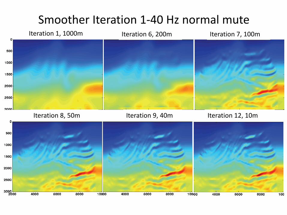
Smoother Iteration 1-40 Hz normal muteIteration 1, 1000m Iteration 6, 200m Iteration 7, 100m

Iteration 8, 50m Iteration 9, 40m Iteration 12, 10m

Data Residual L2 Norms

2 no

rmsid

ual L

2Da

ta re

s

0 5 10 15 20Iteration

Common Image Gather

h3

h1 h2

h3

h1 h2

Smoother Iteration 1-40 Hz wide muteIteration 1, 1000m Iteration 6, 200m Iteration 7, 100m

Iteration 9, 40m Iteration 12, 10mIteration 8, 50m

Smoother Iteration 1-40 Hz harsh muteIteration 1, 1000m Iteration 6, 200m Iteration 7, 100m

Iteration 9, 40m Iteration 12, 10mIteration 8, 50m

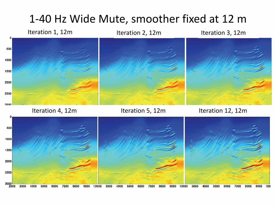
1-40 Hz Wide Mute, smoother fixed at 12 mIteration 1, 12m Iteration 2, 12m Iteration 3, 12m

Iteration 4, 12m Iteration 5, 12m Iteration 12, 12m

Data Residual L2 Norms

2 no

rmsid

ual L

2Da

ta re

s

0 5 10 15 20Iteration

Shot 20Shot 20Original shot

0

Predicted on third iteration

1.0

Seco

nds

2.0

S

4000 6000 8000 4000 6000 8000Meters Meters

Shot 20Shot 20Original shot

0

Predicted by initial model

1.0

Seco

nds

2.0

S

4000 6000 8000 4000 6000 8000Meters Meters

ConclusionsConclusionsThe FTFWI suggests a generalized inversion scheme

with many possible variationswith many possible variations.FWI is an iterative modelling, migration, and

calibration process.pFWI can be done with migration algorithms other

than RTM.Calibration generally involves a wavelet estimation

and scaling, and is reminiscent of impedance inversioninversion.

The process demonstrated here is not claimed to be optimal but is suggestive of many other variantsoptimal, but is suggestive of many other variants.

AcknowledgementsAcknowledgements

W th k i d t f th iWe thank our industry sponsors for their generous support which makes our work possible. We

thank Hussain Hammad for his thesis and discussions.

Calibrating the migrationCalibrating the migration

FTFWI Fi d th l h th tFTFWI: Find the scalar such that

produces the best forward modelled data.

Thi Fi d th l h th tThis paper: Find the scalar such that

where is the well location at which is known.

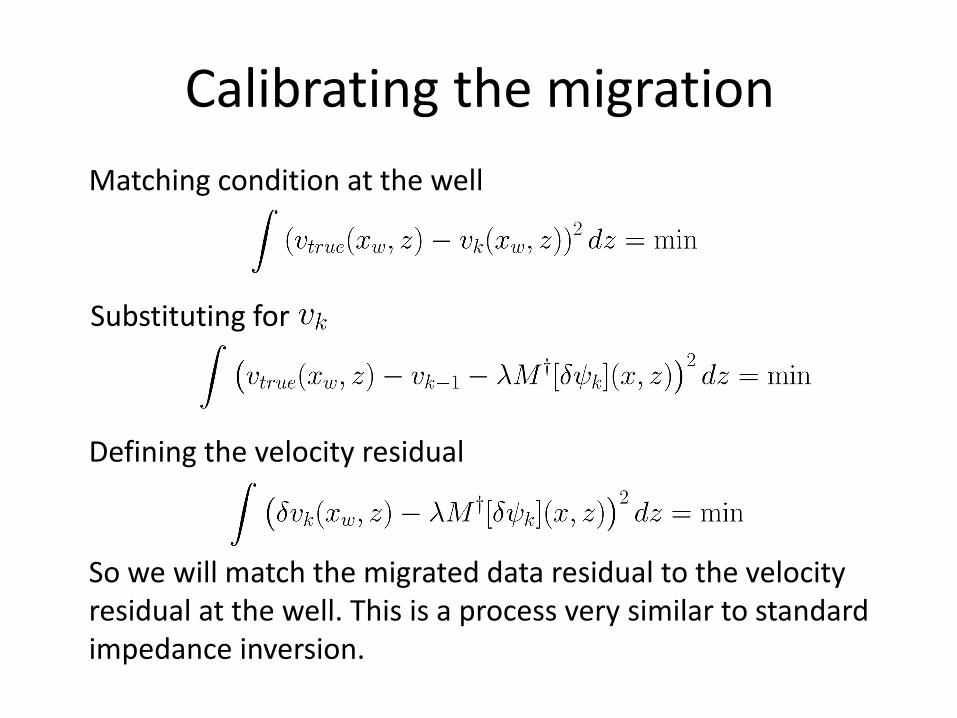
Calibrating the migrationCalibrating the migrationMatching condition at the well

S b tit ti fSubstituting for

Defining the velocity residual

So we will match the migrated data residual to the velocity residual at the well This is a process very similar to standardresidual at the well. This is a process very similar to standard impedance inversion.

WeirdWeird