full field methods and residual stress analysis in orthotropic material. i linear approach

Available online at www.sciencedirect.com

International Journal of Solids and Structures 44 (2007) 8229–8243

www.elsevier.com/locate/ijsolstr

Full field methods and residual stress analysis inorthotropic material. I Linear approach

Antonio Baldi *

Department of Mechanical Engineering, University of Cagliari, Piazza d’Armi, 09123 Cagliari, Italy

Received 26 November 2006; received in revised form 17 March 2007; accepted 14 June 2007Available online 21 June 2007

Abstract

This work analyzes the problem of residual stress determination in an orthotropic material using the hole drilling tech-nique combined with non-contact, full field optical methods. Due to the complex behavior of the material, first a solutionalgorithm for the isotropic case is analyzed, then the procedure is extended to solving the more complex problem. In thefirst part of the work, the simplified Smith–Schajer solution to the through-hole problem for an orthotropic material isanalyzed, showing that the same linear least square approach used in the isotropic case applies to a large set of orthotropicmaterials; based on this analysis a simple residual stress measurement algorithm is developed using either analytical ornumerically estimated calibration coefficients.

In the second part of the work, the general solution is discussed: since in this case the simplified Smith–Schajer solutioncannot be used, the Lekhnitskii’s analysis of the through-hole plate in tension is introduced and extended to handle resid-ual stresses. On this basis a solution algorithm using the nonlinear fit of the theoretical displacement field capable of treat-ing all the orthotropic materials at the cost of a more complex numerical procedure is proposed. The performances of bothalgorithms are tested against numerically generated noisy fields and experimental ones and show a good reliability andaccuracy.� 2007 Elsevier Ltd. All rights reserved.

Keywords: Residual stress; Hole drilling; Orthotropic materials; Smith’s formulation

1. Introduction

Residual stresses usually appear inside mechanical components as a side effect of technological treatment:since they add to stress fields induced by external loads, residual stresses are generally regarded as dangerous.However, this is not always the case: in fact it is common practice to induce opposite sign residual stress fieldsto enhance component strength (e.g. the favourable effect of shot peening on fatigue life).

Whatever the nature of residual stresses inside the component, their detection and measurement is animportant technical issue as engineers need to know the residual (or extra) safety margin resulting from the

0020-7683/$ - see front matter � 2007 Elsevier Ltd. All rights reserved.

doi:10.1016/j.ijsolstr.2007.06.012

* Tel.: +39 070 675 5707; fax: +39 070 675 5717.E-mail address: [email protected]

mailto:[email protected]

8230 A. Baldi / International Journal of Solids and Structures 44 (2007) 8229–8243

stress-inducing treatment. However, since the residual stress field is self-equilibrated, its measurement is noteasy. The researcher either has to rely on some absolute material property (e.g. the inter-crystal distance inX-ray diffraction, or sound speed variation in acoustoelasticity) or disturb the stress balance by removing partof the material. The latter approach is widely used in several forms, from the layer removal technique, to thegroove method, the ring core method or the hole drilling method. The latter is probably the most commonlyused residual stress measuring method (Kandil et al., 2001) and consists essentially of drilling a small hole onthe surface of the component and measuring the strain field induced by material removal, usually by means ofelectrical resistance strain gauges (Rowlands, 1987; Bray, 2001; Lu, 1996).

The hole-drilling strain gauge method is a mature experimental technique (ASTM, 2003) and by using theincremental approach, it also allows measurement of non-uniform stress fields (Schajer, 1988a,b; Zuccarello,1999). Nevertheless, the use of strain gauges is not enforced by this approach and other choices are possible.One attractive alternative is to combine the hole drilling technique with optical non-contact measuring meth-ods. This may provide several advantages: non-contact measurement, no (or reduced) need for preparation ofthe specimen and higher sensitivity.

Following this approach, several optical techniques have been used to measure the strain/displacement fieldaround the hole: from holographic interferometry (Nelson and McCrickerd, 1986; Nelson et al., 1997; Linet al., 1995; Steinzig et al., 2001) to grating interferometry (Nicoletto, 1991; Wu et al., 1998; Wu and Lu,2000; Schwarz et al., 2000; Bulhak et al., 2000) or speckle interferometry (Vikram et al., 1996; Zhang andChong, 1998; Diaz et al., 2000; Albertazzi et al., 2000; Jacquot, 2002; Pechersky and Vikram, 2002; Fochtand Schiffner, 2002; Baldi and Jacquot, 2003; Steinzig and Ponslet, 2003; Viotti et al., 2004).

Although these methods differ largely as to working principle, implementation details and acquired data –holographic interferometry mainly measures out-of-plane displacements, grating interferometry in-plane dis-placements and speckle interferometry one or the other, depending on the optical configuration – they are allnevertheless capable of acquiring full displacement fields so that the optimal use of a huge mass of data toimprove the reliability of the measurement is one of the main topics of these techniques.

Several algorithms to estimate residual stresses from optical data have been proposed in recent years, rang-ing from direct mapping of the standard strain gauge formula (Nelson and McCrickerd, 1986), to the measure-ment of a single displacement component at three points (Nelson et al., 1997; Wu et al., 1998), to themeasurement of the three-dimensional displacement at a single point (Wu and Lu, 2000), the Fourier approx-imation of the X (or Y) component of the displacement on a circle concentric to the hole (Focht and Schiffner,2002) and the least square fitting of the displacement field (Baldi et al., 2003; Steinzig and Ponslet, 2003; Baldi,2005).

However, most of these approaches use only a few data from the displacement field (only Focht and Schiff-ner (2002), Ponslet et al. (2003a), Baldi (2005) and Schajer et al. (2005) explicitly use more than three exper-imental values). Furthermore, their formulation depends heavily on the form of the isotropic displacementfield equations, and consequently most of the methods described above cannot be extended to orthotropic/anisotropic materials.

Recently, a new analysis procedure capable of working with orthotropic material has been proposed (Card-enas-Garcıa et al., 2005). This algorithm is based on the nonlinear least square error minimization between theexperimental data and their analytical representation. The solution algorithm makes full use of all availabledata, but it is unnecessarily complex from a numerical point of view since it was developed in the grating inter-ferometry framework (Cardenas-Garcıa et al., 2006).

This work attempts to use a similar approach by fitting the theoretical displacement field to the experimen-tal data, but without limiting it to the case of grating interferometry. The work is organized in two parts. Inthis first part the simplified Smith–Schajer residual stress formulation is employed, showing that a simple lin-ear least square algorithm can be used for a large class of orthotropic materials, while in the second part ageneral and more complex algorithm is developed.

This first paper is organized as follows: the next section (Section 2) outlines the full-field, least squaremethod for isotropic materials (Steinzig and Ponslet, 2003; Baldi, 2005); an example of modification of theformulation to allow for Albertazzi’s and Kaufmann’s radial sensitivity device (Albertazzi et al., 2000) is alsoshown. In Section 3 the Smith–Schajer solution of the through-hole plate problem for orthotropic materials isanalyzed, showing that when it applies, it can directly replace Kirsch’s solution for isotropic plates (Section 4).

A. Baldi / International Journal of Solids and Structures 44 (2007) 8229–8243 8231

Numerical evaluation (using FEA) of the calibration coefficients is discussed in Section 5, which also revisesthe numerical procedure by taking into account the new formulation. The proposed algorithm is tested in Sec-tion 6 using FEM-generated displacement fields, whereas in Section 7 a simple experimental test to verify theproposed algorithm is shown. A short discussion of the results close the paper (Section 8).

2. Linear least square method for isotropic materials

Consider the data array / acquired using a full field optical method in a residual stress measurement test.Assuming that the ux (uy,uz) displacements can be written as a linear combination of stress components(ux = a11rx + a12ry + a13sxy, uy = a21rx + � � �, where the aij are functions of the material properties, point loca-tion and hole geometry), the least square error between /j, the experimental data at point j, and its interpo-lation can be written as

1 Froj. Usuweight

2 Alldirectidisplac

� ¼XN

j¼1

fwj½kxðjÞuxðjÞ þ kyðjÞuyðjÞ þ kzðjÞuzðjÞ � /j�g2 ð1Þ

where ui(j) is the component i of displacement determined at point j, wj is the measurement reliability at theexperimental point or 1 if unknown,1 and the ki(j) are the components of the sensitivity vector (again atpoint j).2 Writing ux, uy and uz in terms of the stress components, Eq. (1) becomes

� ¼XN

j¼1

fwj½ðkxa11 þ kya21 þ kza31Þrx þ ðkxa12 þ kya22 þ kza32Þry þ ðkxa13 þ kya23 þ kza33Þsxy � /j�g2 ð2Þ

where the explicit dependency on point location of ki and aij has been dropped to simplify the notation.The minimum of the previous expression can easily be determined by differentiating with respect to (w.r.t.)

rx, ry, sxy and setting the derivatives equal to zero. Writing tj = wj(kxa11 + kya21 + kza31), vj = wj(kxa12 +kya22 + kza32) and fj = wj(kxa13 + kya23 + kza33) one finally obtains a linear system

Pj

t2j

Pj

tjvj

Pj

tjfj

Pj

v2j

Pj

vjfj

symm:P

jf2

j

0BBBBB@

1CCCCCA

rx

ry

sxy

8><>:

9>=>;¼

Pj

wjtj/j

Pj

wjvj/j

Pj

wjfj/j

8>>>><>>>>:

9>>>>=>>>>;

ð3Þ

which allows determination of the best fit parameters (the stress components) of the displacement interpolat-ing functions.

Some points should be noted:

• the system (3) interpolates the component of the displacements in the direction of the sensitivity vector(which can also change from point to point). This makes a single acquisition sufficient to determine thestress field;

• the previous formulation is quite general and does not require a specific form of the displacement fields,providing they linearly depend on stress components. For example, if we take into account a pure radialsensitivity speckle interferometry setup (Albertazzi et al., 2000), we have to rewrite the least square errorin terms of radial displacements ur = A(rx + ry) + B[(rx � ry) cos(2h) + 2sxy sin(2h)], obviously droppingthe dependency on ki. By simple algebra it is easy to show that the final system is formally identical to theprevious one (Eq. (3)), but in this case tj = wj[A + B cos(2h)], vj = wj[A � B cos(2h)] and fj = 2B wj sin(2h).

m the statistical point of view, wj should be 1/rj, the inverse of the standard deviation of the measurement at the experimental pointally this datum is not available, but intensity modulation allows estimation of measurement reliability at each point, so that aed summation can be introduced, even though the resulting covariance matrix will not reflect the actual measurement variance.standard optical measuring techniques are capable of acquiring a single component of the displacement (along the sensitivity

on ~k, see Fig. 1), so that obtaining the true displacement requires three separate measurements. However, knowing the completeement field is not necessary, as explained in the following.

2VI2

LaserSource

k2

I1

1V

k1

Z

Y

CCD

ϑr

t

X

Fig. 1. Reference configurations for optical setup. The origin of both cylindrical and orthogonal reference systems is assumed to be on thetop surface, in the centre of the hole. ~k is the sensitivity vector, which in general is not constant since it depends on illumination andviewing angles.


The question now is to verify whether this formulation is general enough to treat orthotropic materials. Tothis aim, first a brief outline of the properties of orthotropic plates will be given, then the least square formu-lation will again be analyzed.

3. Residual stress in through-hole, orthotropic plates (Smith–Schajer solution)

The through-hole plate problem in the general case of anisotropic material was studied by Leknitskii (Lekh-nitskii, 1963, 1968) who adopted Muskhelishvili’s complex variables method (Muskhelishvili, 1934). However,Smith and Schajer (Smith et al., 1944; Schajer and Yang, 1994; Cardenas-Garcıa et al., 2005) showed that asimpler, real-value formulation can be used for a large class of materials; according to these authors, in aorthotropic material the displacement field due to residual stresses release can be written as

ux ¼ Ax½Y 1ð1þ bmÞsxy � X 1ðrx � bmryÞ� þ Bx½Y 2ð1þ amÞsxy � X 2ðrx � amryÞ� ð4Þuy ¼ Ay ½X 1ð1þ bmÞsxy þ Y 1ðrx � bmryÞ� þ By ½X 2ð1þ amÞsxy þ Y 2ðrx � amryÞ� ð5Þ

where the Ax, . . . ,By parameters are (note the use of myx in Ay and By)

Ax ¼ ½ðamÞ2 þ mxy �=½mðb� aÞExxð1� amÞ�Bx ¼ ½ðbmÞ2 þ mxy �=½mða� bÞExxð1� bmÞ�Ay ¼ ½1þ ðamÞ2myx�=½am2ðb� aÞEyyð1� amÞ�By ¼ ½1þ ðbmÞ2myx�=½bm2ða� bÞEyyð1� bmÞ�

whereas the a, b, m and j material parameters are

m ¼ffiffiffiffiffiffiffiffiffiffiffiffiffiffiffiExx=Eyy

4

qj ¼ 1

2

ffiffiffiffiffiffiffiffiffiffiffiffiffiExxEyy

p½1=Gxy � ð2mxyÞ=Exx�

a ¼ffiffiffiffiffiffiffiffiffiffiffiffiffiffiffiffiffiffiffiffiffiffiffiffiffiffijþ

ffiffiffiffiffiffiffiffiffiffiffiffiffij2 � 1pq

b ¼ffiffiffiffiffiffiffiffiffiffiffiffiffiffiffiffiffiffiffiffiffiffiffiffiffiffij�

ffiffiffiffiffiffiffiffiffiffiffiffiffij2 � 1pq

and the ‘‘geometric’’ parameters are

TableChara

Materi

Glass-BoronGraphPlywooPlywooPlywoo

Theo.Theo.

Theo.

The m


X 1 ¼ x� W 1 cos w1 X 2 ¼ x� W 2 cos w2

Y 1 ¼ amy� W 1 sin w1 Y 2 ¼ bmy� W 2 sin w2

W 1 ¼ffiffiffiffiffiffiffiffiffiffiffiffiffiffiffia2

1 þ b21

4

qW 2 ¼

ffiffiffiffiffiffiffiffiffiffiffiffiffiffiffia2

2 þ b22

4

q

a1 ¼ x2 � r2a � ðamÞ2ðy2 � r2

aÞ b1 ¼ 2amxy

a2 ¼ x2 � r2a � ðbmÞ2ðy2 � r2

aÞ b2 ¼ 2bmxy

w1 ¼ 12

arctanðb1=a1Þ w2 ¼ 12

arctanðb2=a2Þ

ra being the radius of the hole.Note that to obtain correct results both w1 and w2 must lie in the same quadrant of arctan(y/x). Moreover

this formulation requires j to be greater than 1 (see the expression of a and b). This means that Eqs. (4) and (5)cannot be used for all orthotropic materials (in fact the j > 1 requirement puts a limitation on the normalizedsize of Gxy, see the definition of j); however, except for composites specifically designed for high shear stiffness,this condition is usually satisfied (see Table 1 for a list of materials).

Figs. 2–4 show how orthotropy modifies the displacement field by comparing one isotropic and two ortho-tropic plates subjected to the same load (rx = �ry = 1, sxy = 0). Note that the first orthotropic material (agraphite/boron composite) is moderately anisotropic (j = 4.65) while the second (a hypothetical, but thermo-dynamically admissible material) is highly anisotropic (j = 9.75).

1cteristic parameters of some materials (Schimke et al., 1968; Savin, 1961)

al E11/E22 m12 G12/E22 j

epoxy 2.99 0.25 0.5 1.58-epoxy 10.0 0.3 0.33 4.65ite-epoxy 40.01 0.25 0.5 6.29d 1 3.86 0.59 0.74 1.02d 2 24.6 0.3 0.75 3.25d 3 1.0 0.77 2.04 �0.53

1 1.5 0.37 0.4 1.222 20.0 1.0 10.0 0.0

3 1.0 0.25 0.05 9.75

aterials in boldface cannot be analysed using Smith’s formulation.

X [mm]

Y [m

m]

-15 -10 -5 0 5 10 15

-15

-10

-5

0

5

10

15

X [mm]

Y [m

m]

-15 -10 -5 0 5 10 15

-15

-10

-5

0

5

10

15

Fig. 2. Displacement field around a hole in an isotropic material. Left ux, right uy. rx = �ry = 1, sxy = 0.

X [mm]

Y [m

m]

-15 -10 -5 0 5 10 15

-15

-10

-5

0

5

10

15

X [mm]

Y [m

m]

-15 -10 -5 0 5 10 15-15

-10

-5

0

5

10

15

Fig. 3. Displacement field around a hole in an orthotropic material. Left ux, right uy (E1/E2 = 10.0, G12/E2 = 0.33, m12 = 0.3, j = 4.65).Loads are the same as in Fig. 2 (rx = �ry = 1, sxy = 0). The principal axes of material are along the X and Y directions.

X [mm]

Y [m

m]

-15 -10 -5 0 5 10 15

-15

-10

-5

0

5

10

15

X [mm]

Y [m

m]

-15 -10 -5 0 5 10 15

-15

-10

-5

0

5

10

15

Fig. 4. Displacement field around a hole in an orthotropic material. Left ux, right uy (E1/E2 = 1, G12/E2 = 0.05, m12 = 0.25, j = 9.75). Notethat these values are not related to a real material, but they are thermodynamically admissible. Loads are the same as in Fig. 2(rx = �ry = 1, sxy = 0). The principal axes of material are along the X and Y directions.


4. Linear least square approach for orthotropic materials

Eqs. (4) and (5) can be rearranged in the following form:

ux ¼ �ðAxX 1 þ BxX 2Þrx þ mðbAxX 1 þ aBxX 2Þry þ ½ð1þ mbÞAxY 1 þ ð1þ maÞBxY 2�sxy

uy ¼ þðAyY 1 þ ByY 2Þrx � mðbAyY 1 þ aByY 2Þry þ ½ð1þ mbÞAyX 1 þ ð1þ maÞByX 2�sxyð6Þ

explicitly showing that the displacement components linearly depend on stress components; this means thatthe requirements of the least square approach of Section 2 are satisfied. Eq. (2) still holds, providing thatthe out-of-plane components are removed

� ¼XN

j¼1

fwj½ðkxa11 þ kya21Þrx þ ðkxa12 þ kya22Þry þ ðkxa13 þ kya23Þsxy � /j�g2 ð7Þ

where the explicit dependencies on point location have been dropped and the aik(j) coefficients can be esti-mated from Eq. (6):


a11 ¼ �ðAxX 1 þ BxX 2Þa12 ¼ mðbAxX 1 þ aBxX 2Þa13 ¼ ð1þ mbÞAxY 1 þ ð1þ maÞBxY 2

a21 ¼ ðAyY 1 þ ByY 2Þa22 ¼ mðbAyY 1 þ aByY 2Þa23 ¼ ð1þ mbÞAyX 1 þ ð1þ maÞByX 2

ð8Þ

The solution system can be obtained by differentiating Eq. (7) w.r.t. the rx, ry and sxy stress components andposing the derivatives equal to zero. Writing

tj ¼ �wj½kxðAxX 1 þ BxX 2Þ � kyðAyY 1 þ ByY 2Þ�vj ¼ mwj½kxðbAxX 1 þ aBxX 2Þ � kyðbAyY 1 þ aByY 2Þ�fj ¼ wjfky ½ð1þ mbÞAyX 1 þ ð1þ maÞByX 2�

þ kx½ð1þ mbÞAxY 1 þ ð1þ maÞBxY 2�g

ð9Þ

the linear solution system (3) still holds.Thus the solution procedure for residual stress identification in orthotropic materials is exactly the same as

for isotropic materials, except that the Kirsch-related terms of Eq. (3) have to be replaced with those ofSmith’s (i.e. Eq. (9)).

However, it must be pointed out that the Smith–Schajer solution takes into account the in-plane compo-nents only. This means that if the sensitivity vector does not lie in the plane, the proposed algorithm cannotbe directly used to analyze the acquired data. Thus either an experimental technique giving pure in-plane dis-placements has to be used or more than one displacement field has to be acquired, thus allowing an estimate(and numerical removal) of the out-of-plane component.

4.1. Singular value decomposition approach

The linear dependency of displacement from stress components allows replacement of the normal equationformulation with the numerically more robust Singular Value Decomposition (SVD) one. In fact, it is wellknown that SVD produces a solution that minimizes the residual r = |Ax � b| in the least square sense inthe case of over-determined systems (Press et al., 1992). To use the SVD approach we have to:

(1) build the A matrix and the known term vector b; each row i of A being theffiffiffiffi�ip

(that is, Ai1 = kxa11(i) +kya21(i), Ai2 = kxa12(i) + kya22(i), Ai3 = kxa13(i) + kya23(i)); A thus results as a N · 3 matrix;

(2) decompose A by SVD, obtaining A = U Æ D Æ V where U is a N · 3 matrix, D is a 3 · 3 diagonal matrix(containing the singular values xj) and V is a 3 · 3 orthonormal matrix;

(3) (if necessary) nullify the vanishing elements of D (to remove null space components);(4) solve the system by back-substitution x = V[diag(1/xj)] Æ (UTb).

Note that the procedure described above is usually implemented as a library function, so that only the errorfunction estimating the terms of A at point i has to be user-implemented; moreover, the derivatives of the errorfunction w.r.t. the fitting parameters need not be evaluated. On the negative part, this approach requires someextra storage and more computing power.

5. Numerical evaluation of calibration coefficients

Since in orthotropic materials residual stresses depend on material properties and location, it may be usefulto evaluate the coefficients of Eq. (6) using a numerical, Finite Element-based (FEM), approach. To this end,it is best to rewrite the displacement components in compact form


ux ¼ a11rx þ a12ry þ a13sxy

uy ¼ a21rx þ a22ry þ a23sxyð10Þ

where a11, . . . ,a23 play the same role as the calibration coefficients A . . .F of the isotropic case and depend onmaterial properties and point location.

Eq. (10) shows that since each FEM calculation estimates both X and Y displacements, at least three runsare required. It is quite easy to identify a set of load combinations that allows evaluation of a11 . . .a23, becauseeach stress component affects one calibration coefficient only; however, aiming at using the same code as in theisotropic case, the following three loading cases appear to be the most appropriate:

(1) a simple hydrostatic loading case (rx = ry = P, sxy = 0); by substituting the stress components in (10)one obtains

uhx ¼ ða11 þ a12ÞP

uhy ¼ ða21 þ a22ÞP

ð11Þ

where the h index points out the loading case.(2) a shear case (rx = �ry = P, sxy = 0); by substituting in (10) the displacement components become

usx ¼ ða11 � a12ÞP

usy ¼ ða21 � a22ÞP

ð12Þ

(3) a second shear case (rx = ry = 0, sxy = P), which allows direct estimation of a13 and a23; in fact, usingthis load configuration, Eq. (10) reduces to ut

x ¼ a13P and uty ¼ a23P .

The a11, a12, a21 and a22 coefficients can be estimated by summing and subtracting Eqs. (11) and (12), thusobtaining

a11 ¼ ðuhx þ us

xÞ=ð2P Þ a12 ¼ ðuhx � us

xÞ=ð2P Þa21 ¼ ðuh

y þ usyÞ=ð2P Þ a22 ¼ ðuh

y � usyÞ=ð2P Þ

Note that the first and second loading configurations are exactly the same as in the isotropic case. On the con-trary, due to the loading conditions, the FE mesh cannot be the ‘‘standard’’ quarter of a circle commonly usedin the isotropic case and a full circular mesh has to be employed. Fig. 5 shows how the FEM solution con-verges to the Smith–Schajer theoretical result in terms of the identified residual stress values (that is, it showsthe percent errors between the estimated and expected result when FEM-generated displacement fields areanalyzed using theoretical estimated calibration coefficients). Since the code used (MSC Marc 2005r2) doesnot include semi-infinite, plane stress elements, two different sets of boundary conditions have been consid-ered: a fully constrained external circle and a tangential only constraint applied to all nodes of the externalboundary. Elements employed were four nodes, plane stress elements and the full circle was divided into 80parts. The expected result was a 45� oriented residual stress field, which seems to be a critical configuration(see Figs. 7 and 8).

As usual (Wu et al., 1998; Ponslet et al., 2003b; Baldi, 2005), residual stress are simulated by applying loadson hole boundaries. Thus the two isotropic-like coefficient pairs can be estimated by applying a radial stressrr = �P on the hole boundary and a radial stress rr = �P cos(2#) coupled with a shear stress sr# = +P sin(2#)on the hole boundary. The latter loading configuration requires application of rr = �P sin(2#) and sr# = �P

cos(2#) on the hole boundary. Contrary to the case of isotropic materials, the calibration coefficients are notradially symmetric; thus they must be evaluated for each measurement point.

Using calibration coefficients combined with the SVD approach, the residual stress estimation procedurebecomes:

(1) Perform FEM simulations using the material parameters of the specimen under investigation and esti-mate calibration coefficients a11 . . .a23 as previously described (alternatively the calibration coefficientscan be estimated using Eq. (8));

0

2

4

6

8

10

12

14

16

18

20

22

10 15 20 25 30 35 40 45

abs(

σ 1te

o - σ

1num

) [%

]

external- to hole-radius ratio

fulltangential

Fig. 5. Convergence of the FEM-evaluated displacement field to the theoretical one in terms of percent error of the estimated residualstress. A fully constrained and a tangential-only constrained external circle were considered. Expected residual stress is r1 = 100 MPa at45�.


(2) Assemble the A matrix and the known terms vector b as described in Section 4.1.(3) Decompose A using SVD, remove vanishing null space components (if required) and perform back-sub-

stitution to obtain the residual stress components.

If the normal equation method is used, steps 2 and 3 have to be replaced by the estimation of the normalequation solution system Eq. (3) and by a standard linear system solution.

6. Numerical experiments

To verify the performance of the proposed algorithm, some tests were performed on numerically generateddisplacement fields (both noisy and noise-free). Although Eqs. (4) and (5) allow easy estimation of the u and v

displacement fields for any loading configuration, their use does not ensure against code mis-implementations,so that we opted for using FEM-generated input data. To this end, a circular mesh was built using four nodes,plane stress elements. The hole- to the external-radius ratio was 20; all nodes on the outer circle were con-strained in the tangential direction while the loads were applied on the hole boundary (thus, looking atFig. 5, errors between 2% and 4% are to be expected on noise-free images). Moreover, to reduce the influenceof boundary constraints, the two external rings of elements were discarded.

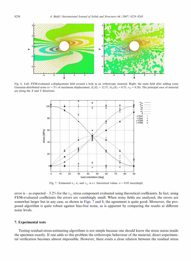
Fig. 6 (left) shows the FEM-evaluated u displacement field near the hole when the applied loads arerx = 75 MPa, ry = 25 MPa, sxy = 43.3 MPa (r1 = 100 MPa, u = 30�, E1 = 93.7 GPa, E2 = 7.45 GPa,m12 = 0.26, G12 = 3.98 GPa), while Fig. 6 (right) shows the same field after inserting some noise (a Gaussiandistributed additive noise was used, with no bias and a standard deviation equal to 5% of the maximumdisplacement).

Several loading conditions were tested (r1 = 100 MPa, r2 = 0, u = 0, 15, 30, . . . , 90�), with increasing noiselevels (0%, 5%, 10% of maximum displacement) and were evaluated using either the u or the v displacementcomponents, with theoretical- or FEM-evaluated coefficients.

Figs. 7 and 8 show the evaluated stress as a function of the load orientation when the standard deviation ofthe noise corresponds respectively to 5% and 10% of maximum displacement. The lines represent the theoret-ical behaviour of the stress components when load orientation changes, while the various symbols report theestimated residual stress components using the four software configurations taken into account (theoretical/FEM-calibrated coefficients, u/v displacements). On examining the noise-free results (not shown) the larger

X

Y

-4 -2 0 2 4

-4

-2

0

2

4

X

Y

-4 -2 0 2 4

-4

-2

0

2

4

Fig. 6. Left: FEM-evaluated u-displacement field around a hole in an orthotropic material. Right: the same field after adding someGaussian-distributed noise (r = 5% of maximum displacement, E1/E2 = 12.57, G12/E2 = 0.53, m12 = 0.26). The principal axes of materialare along the X and Y directions.

0

20

40

60

80

100

0 10 20 30 40 50 60 70 80 90

stre

ss [M

Pa]

load orientation [deg]

σxxσyyτxyσ1σ2

θu theov theou FEMv FEM

Fig. 7. Estimated rx, ry and sxy w.r.t. theoretical values. r = 0.05 max(displ).


error is – as expected – 3.2% for the sxy stress component evaluated using theoretical coefficients. In fact, usingFEM-evaluated coefficients the errors are vanishingly small. When noisy fields are analyzed, the errors aresomewhat larger but in any case, as shown in Figs. 7 and 8, the agreement is quite good. Moreover, the pro-posed algorithm is quite robust against bias-free noise, as is apparent by comparing the results at differentnoise levels.

7. Experimental tests

Testing residual-stress-estimating algorithms is not simple because one should know the stress status insidethe specimen exactly. If one adds to this problem the orthotropic behaviour of the material, direct experimen-tal verification becomes almost impossible. However, there exists a close relation between the residual stress

0

20

40

60

80

100

0 10 20 30 40 50 60 70 80 90

stre

ss [M

Pa]

load orientation [deg]

σxxσyyτxyσ1σ2

θu theov theou FEMv FEM

Fig. 8. Estimated rx, ry and sxy w.r.t. theoretical values. r = 0.10 max(displ).


field around a hole and the corresponding distribution on an infinite plate with a hole under tension: in fact, itis possible to obtain one from the other by summing (subtracting) the displacement field of a plane in tension.Using this observation, a semi-experimental verification can be performed in the following way:

(1) drill the hole in the specimen; in this way the residual stresses, if present, are released;(2) acquire the reference phase modulo 2p field;(3) apply a known load (either by using a load cell or with a strain gauge glued to the specimen far from the

hole) and acquire the new phase field;(4) subtract the two displacement fields and unwrap the result;(5) subtract from the experimental displacement field the solution of an infinite plane in tension (note the myx

in upy ):

upx ¼

rx � mxyry

Exxxþ sxy

2Gxyy

upy ¼

sxy

2Gxyxþ ry � myxrx

Eyyy

(6) use the resulting displacement field as the input data for the residual-stress-estimating algorithm.

Depending on the unwrapping algorithm used, a mask has to be built in step 4 to allow performing phaseunwrapping.

The always present rigid body translations and rotations have to be subtracted from the experimental databefore performing the analysis. Since a rigid body rotation results in a linear component added to the originaldisplacement field, if its subtraction (by least square fitting of a plane in the experimental data) is performedimmediately after data acquisition, the correction of step 5 is no longer required. Note that instead of perform-ing a separate fit, this operation can also be included in the global formulation by adding three auxiliary vari-ables to the system (3), taking into account rigid body motion components. See Ponslet et al. (2003a), Schajeret al. (2005) for details.

A standard in-plane-sensitivity speckle interferometry setup was used to acquire the displacement field(Fig. 9), with a HeNe laser source (k = 632.8 nm) and an illumination angle h = 30� (so that sensitivity s

results 0.6328 lm/fringe). Even though it was not strictly needed, a residual stress-specific sample holder

PZ

T

SP

SH

BS

CCD

LS

BE

BE

M

M

α

Fig. 9. ESPI in-plane sensitivity setup. SP, specimen; SH, sample holder; BE, beam expander; LS, laser source; PZT, piezo translator;CCD, camera; M, mirror; BS, beam splitter.


was used to mimic the real experiment. In fact, in the standard hole drilling technique, the drilling machinemakes it impossible to have a full field of view, thus either the specimen or the drill has to be moved. Followingour previous experience (Baldi and Jacquot, 2003), the first choice was selected and a special isostatic sampleholder was designed and built (see Figs. 10 and 11). This consists of three elements: the real sample holder, afixed support mounted on the optical bench and a reference plate installed in the drilling machine (actually a

Fig. 10. Sample holder. Left: removable plate; right: support used on the optical bench (note the back sphere, the v-groove and thereference hole). The removable plate is mounted in the support using two of the four balls installed on it and the sphere mounted in thefixed support, thus creating an isostatic connection. Using different pairs of balls, two orthogonal sensitivity directions can be acquired.

Fig. 11. Sample holder. Left: fixed plate (to be installed in the milling machine); right: the removable plate mounted on the optical bench.


numerically controlled milling machine equipped with a 3D touch probe). Since the precision requirement forthe optical setup and the drilling machine are different, the sample holder is connected to the plate installed onthe milling machine using screws and pins; on the contrary, to ensure the sub-micrometric repositioning accu-racy required by the optical system, a kinematic system was created using a point-line-plane configuration: thesample holder is equipped with a pair of balls which are inserted in a hole (thus defining a point) and a v-groove (defining a line) in the fixed support on the optical bench. A ball mounted in the support realizes asingle-side constraint on the back of the sample holder thus making the configuration unique. Actually thesample holder is equipped with two pairs of balls, so that it is possible to acquire two displacement fieldsin orthogonal directions.

The sample holder allows application of several type of loads to the specimen. In fact, both the specimenclamps can be moved using a screw system mounted inside the plate (the right one in the horizontal direction,the left one in the vertical direction); a floating element in the centre of the plate allows application of out-of-plane loads (part of this system, located on the back of the sample holder, is not shown in the figures).

Fig. 12 shows the experimental displacement field acquired in a unidirectional graphite/peek laminate(E11 = 133.8 GPa, E22 = 8.9 GPa, m12 = 0.3, G12 = 5.1 GPa, j = 6.61) using the setup described above.Fig. 13 shows the wrapped phase field after rigid body subtraction. Using the proposed least square algorithm,the estimated stress components are rx = 9.16 MPa, ry = 0.08 MPa, sxy = 0.17 MPa, which shows a goodagreement with the expected value (rx = 8.45 MPa, ry = sxy = 0.).

Fig. 12. u displacement field (actually wrapped phase) around a hole in a graphite/peek unidirectional laminate before rigid body removal.The equivalent residual stress is rx = 8.45 MPa.

Fig. 13. u displacement field (actually wrapped phase) around a hole after subtraction of the planar displacement field.


8. Conclusions

Determining residual stress in orthotropic materials is, in the general case, much more difficult than in iso-tropic materials. However, in this paper it has been shown that if one accepts a somewhat more involvedexpression of the calibration coefficient, the ‘‘standard’’ least square approach used for isotropic materialcan be extended to a large class of orthotropic materials (j > 1), thus generating a solution system which isstill linear. The numerical and experimental verification performed shows that the method is capable of pro-viding reliable results even when a significant noise level is present.

Solving the general case requires a more involved procedure and generates a nonlinear solution system.This point will be discussed in depth in the second part of this work.

References

Albertazzi, A.J., Kanda, C., Borges, M.R., Hrebabetzky, F., 2000. A radial in-plane interferometer for espi measurement. In: Kujawinska,M., Pryputniewicz, R.J., Takeda, M. (Eds.), Laser interferometry X. Techniques and Analysis. Vol. 4101 of Proceedings of SPIE,Bellingham, Washington, pp. 77–88.

ASTM, 2003. Standard test method for determining residual stresses by the hole-drilling strain-gage method (e837-01e1). In: Annual Bookof ASTM Standards. Vol. 03-01. ASTM, West Conshohocken, PA.

Baldi, A., 2005. A new analytical approach for hole drilling residual stress analysis by full field method. Journal of Engineering Materialsand Technology 127 (2), 165–169.

Baldi, A., Jacquot, P., 2003. Residual stresses investigations in composite samples by speckle interferometry and specimen repositioning.In: Gastinger, K., Løkberg, O.J., Winther, S. (Eds.), Speckle Metrology 2003. Vol. 4933 of Proceedings of SPIE, Bellingham,Washington, pp. 141–148.

Baldi, A., Bertolino, F., Ginesu, F., 2003. On the residual stress measurement using the hole-drilling method: calculation algorithms forfull-field experimental techniques. In: AIAS 2003, Atti del XXXII Convegno AIAS. AIAS, Fisciano (SA), Italy, in Italian.

Bray, D.E. (Ed.), 2001. Residual Stress Measurement and General Nondestructive Evaluation. Vol. PVP 429. American Society ofMechanical Engineering, Pressure Vessels and Piping Division.

Bulhak, J., Lu, J., Montay, G., Surrel, Y., Vautrin, A., 2000. Grating shearography and its application to residual stress evaluation. In:Jacquot, P., Fournier, J.M. (Eds.), Interferometry in Speckle Light: Theory and Applications. Springer, Berlin, pp. 607–614.

Cardenas-Garcıa, J.F., Ekwaro-Osire, S., Berg, J.M., Wilson, W.H., 2005. Non-linear least-square solution to the moire hole methodproblem in orthotropic materials. Part i: residual stresses. Experimental Mechanics 45 (4), 301–313.

Cardenas-Garcıa, J.F., Preidikman, S., Shabana, Y.M., 2006. Solution of the moire hole drilling method using a finite-element-method-based approach. International Journal of Solids and Structures 46 (22–23), 6751–6766.

Diaz, F.V., Kaufmann, G.H., Galizzi, G.E., 2000. Determination of residual stresses using hole drilling and digital speckle patterninterferometry with automated data analysis. Optics and Lasers in Engineering 33 (1), 39–48.

Focht, G., Schiffner, K., 2002. Numerical processing of measured full-field displacement data around holes for residual stressdetermination. In: Mang, H.A., Rammerstorfer, F.G., Eberhrdsteiner, J. (Eds.), Fifth World Congress on Computational Mechanics,Vienna, Austria.

Jacquot, P., 2002. Pratiques actuelles en analyse de deformation par voie optique: exemple des contraintes residuelles. In: Caracterisationexperimentale des contraintes: techniques avancees et nouveaux materiaux, Troyes cedex, France, pp. 20–30.

Kandil, F.A., Lord, J.D., Fry, A.T., Grant, P.V., 2001. Review of residual stress measurement methods – a guide to technique selection.Tech. Rep. MATC(A)04, National Physical Laboratory, http://www.npl.co.uk/materials/residualstress/npl_publications.html, projectCPM4.5, Measurement of Residual Stress in Components.

Lekhnitskii, S.G., 1963. Theory of Elasticity of an Anistotropic Elastic Body. Holden-day, translation of 1950 Russian ed.Lekhnitskii, S.G., 1968. Anisotropic plates. Gordon and Breach Science Publisher, translation of 1957 Russian ed.Lin, S.T., Hsieh, C.-T., Lee, C.K., 1995. Full field phase-shifting holographic blind-hole techniques for in-plane residual stress detection.

In: Honda, T. (Ed.), International Conference on Applications of Optical Holography. Vol. 2577 of Proceedings of SPIE. Bellingham,Washington, pp. 226–237.

Lu, J., 1996. Handbook of Measurement of Residual Stresses. The Fairmont Press, Inc., Lilburn, GA.Muskhelishvili, N.I., 1934. A new general method of the solution of the fundamental boundary value problems of the plane theory of

elasticity. Dikl. Akad. Nauk SSSR 3 (1), 7–11.Nelson, D.V., McCrickerd, J.T., 1986. Residual-stress determination through combined use of holographic interferometry and blind hole

drilling. Experimental Mechanics 26, 371–378.Nelson, D.V., Makino, A., Fuchs, E.A., 1997. The holographic-hole drilling method for residual stress determination. Optics and Lasers in

Engineering 27, 3–23.Nicoletto, G., 1991. Moire interferometry determination of residual stresses in presence of gradients. Experimental Mechanics 31 (3), 252–

256.Pechersky, M.J., Vikram, C.S., 2002. Enhanced measurement of residual stress by speckle correlation interferometry and local heat

treating for low stress levels. Journal of Pressure Vessel Technology – Transactions of the ASME 124 (3), 371–374.

http://www.npl.co.uk/materials/residualstress/npl_publications.html


Ponslet, E., Steinzig, M., 2003a. Residual stress measurement using the hole drilling method and laser speckle interferometry part ii:analysis technique. Experimental Techniques 27 (4), 17–21.

Ponslet, E., Steinzig, M., 2003b. Residual stress measurement using the hole drilling method and laser speckle interferometry part iii:analysis technique. Experimental Techniques 27 (5), 45–48.

Press, W.H., Teukolsky, S.A., Vetterling, W.T., Flannery, B.P., 1992. Numerical Recipes in C. The Art of Scientific Computing, second ed.Cambridge University Press.

Rowlands, R.E., 1987. Residual stresses. In: Kobayashi, A.S. (Ed.), Handbook on Experimental Mechanics. Prentice-Hall, Inc.,Englewood Cliffs, New Jersey, pp. 768–813, Chapter 18.

Savin, G.N., 1961. Stress Concentration Around Holes. Pergamon Press, translation of 1951 Russian ed.Schajer, G.S., 1988a. Measurement of non-uniform residual stresses using the hole-drilling method. part i – stress calculation procedures.

Journal of Engineering Materials and Technology 110 (4), 338–343.Schajer, G.S., 1988b. Measurement of non-uniform residual stresses using the hole-drilling method. Part ii – practical application of the

integral method. Journal of Engineering Materials and Technology 110 (4), 344–349.Schajer, G.S., Steinzig, M., 2005. Full-field calculation of hole drilling residual stresses from electronic speckle pattern interferometry data.

Experimental Mechanics 45 (6), 526–532.Schajer, G.S., Yang, L., 1994. Residual-stress measurement in orthotropic materials using the hole-drilling method. Experimental

Mechanics 34 (4), 324–333.Schimke, J., Thomas, K., Garrison, J., 1968. Approximate Solution of Plane Orthotropic Elasticity Problems. Management Information

Services, Detroit, Michigan.Schwarz, R.C., Kutt, L.M., Papazian, J.M., 2000. Measurement of residual stress using interferometric moire: a new insight. Experimental

Mechanics 40 (3), 271–281.Smith, C.B., May 1944. Effect of elliptic or circular holes on the stress distribution in plates of wood or plywood considered as orthotropic

materials. Tech. Rep. Mimeo 1510, USDA Forest Products Laboratory, Madison, WI.Steinzig, M., Ponslet, E., 2003. Residual stress measurement using the hole drilling method and laser speckle interferometry: part i.

Experimental Techniques 27 (3), 43–46.Steinzig, M., Hayman, G., Rangaswamy, P., 2001. Data reduction methods for digital holographic residual stress measurement. In:

Proceedings of the 2001 SEM Annual Conference and Exposition on Experimental and Applied Mechanics. Portland, OR.Vikram, C.S., Pechersky, M.J., Feng, C., Engelhaupt, D., 1996. Residual-stress analysis by local laser heating and speckle-correlation

interferometry. Experimental Techniques 20 (6), 27–30.Viotti, M.R., Albertazzi, A.J., Kaufmann, G.H., 2004. Residual stress measurement using a radial in-plane speckle interferometer and

laser annealing: preliminary results. Optics and Lasers in Engineering 42 (1), 71–84.Wu, Z., Lu, J., 2000. Study of surface residual stress by three-dimensional displacement data at a single point in hole drilling method.

Journal of Engineering Materials and Technology 122 (2), 215–220.Wu, Z., Lu, J., Han, B., 1998. Study of residual stress distribution by a combined method of moire interferometry and incremental hole

drilling, part i: theory. Journal of Applied Mechanics 65 (4), 837–843.Zhang, J., Chong, T.C., 1998. Fiber electronic speckle pattern interferometry and its applications in residual stress measurements. Applied

Optics 37 (27), 6707–6715.Zuccarello, B., 1999. Optimal calculation steps for the evaluation of residual stress by the incremental hole drilling method. Experimental

Mechanics 39 (2), 117–124.

full field methods and residual stress analysis in orthotropic material. i linear approach

Documents