Full Block J-Jacobi Method for Hermitian MatricesI

Vjeran Haria,∗, Sanja Singerb, Sasa Singera

aFaculty of Science, Department of Mathematics, University of Zagreb, Bijenicka cesta 30, 10000 Zagreb,Croatia

bFaculty of Mechanical Engineering and Naval Architecture, University of Zagreb, I. Lucica 5, 10000Zagreb, Croatia

Abstract

The paper considers convergence, accuracy and efficiency of a block J-Jacobi method.The method is a proper BLAS 3 generalization of the known method of Veselic forcomputing the hyperbolic singular value decomposition of rectangular matrices. At eachstep, the proposed algorithm diagonalizes the block-pivot submatrix. The convergenceis proved for cyclic strategies which are weakly equivalent to the row-cyclic strategy.The relative accuracy is proved under the standard conditions. Numerical tests showimproved performance with respect to the block-oriented generalization of the originalmethod of Veselic. Combined with the Hermitian indefinite factorization, the proposedmethod becomes accurate and efficient eigensolver for Hermitian indefinite matrices.

Keywords: block J–Jacobi method, convergence, accuracy2000 MSC: 65F15, 65Y20, 46C20

1. Introduction

In this paper we consider a block J-Jacobi method for solving the eigenvalue prob-lem for the pair (A, J), where A is Hermitian positive definite and J is the diagonalmatrix of signs. The method is a proper block generalization of the known methodof Veselic [39], which has been proposed for definite matrix pairs (H, J), H Hermi-tian. The convergence and accuracy properties of that simple method have been studiedin [39, 12, 26] and [34, 35], respectively.

The most natural application of the Veselic method lies in its use in the compoundmethod for accurate computation of the eigenvalues and eigenvectors of an indefinite

IThis work was supported by grants 037–0372783–3042 and 037–1193086–2771 by Ministry of Sci-ence, Education and Sports, Croatia.

∗Corresponding author.Email addresses: hari@math.hr (Vjeran Hari), ssinger@math.hr (Sanja Singer),

singer@math.hr (Sasa Singer)Preprint submitted to Linear Algebra Appl. February 28, 2012

Hermitian (or symmetric) matrix of order n. The first part of the method computes theindefinite factorization of the Hermitian matrix H, by a variant of the Bunch–Parlettfactorization (see [7, 3, 4, 6, 5, 1]), while the second part computes the eigenvalues andeigenvectors of the positive definite pair (A, J), A = G∗G. Here G is the full columnrank m × n matrix obtained from the indefinite factorization H = GJG∗. In [21] wehave explained with more details how G is obtained from H. We believe that the bestway how to solve the obtained generalized eigenproblem is to compute the hyperbolicsingular value decomposition (HSVD) of G (see [2]), by using one-sided version of theJacobi-type algorithm of Veselic [39]. We shall refer to it as J-Jacobi algorithm. Thismethod has been proved to be relatively accurate [35].

If G is any m × n matrix with m ≥ n, the HSVD of G with respect to J, has the form

G = U[

Σ

0

]V∗, Σ = diag(σ1, σ2, . . . , σn), σ1 ≥ σ2 ≥ · · ·σn ≥ 0,

where U is m × m unitary, Σ is the matrix of hyperbolic singular values, and V is n × nJ-unitary matrix, which satisfies V∗JV = J. If G is the factor of the Hermitian indefinitematrix H, H = GJG∗, then using the HSVD, we have

H = GJG∗ = U[

Σ

0

]V∗JV

[Σ 0

]U∗ = U diag(JΣ2, 0)U∗.

Hence, the squares of the hyperbolic singular values of G are, up to the signs in J, thenonzero eigenvalues of H, and U is the corresponding eigenvector matrix. The methodbecomes more efficient if J has the form diag(Iν,−In−ν) where 1 ≤ ν ≤ n − 1. This canbe achieved by the congruence transformation (G∗G, J) 7→ (P∗1G∗GP1, P

∗1JP1) with a

suitable permutation matrix P1.If G is “well-behaved”, i.e., if small relative changes in the elements of G can cause

only small relative changes in the hyperbolic singular values and vectors, then the one-sided algorithm of Veselic will compute them with an appropriate relative accuracy. Inparticular, if the condition number of G∆ is small for some nonsingular diagonal ∆, thenthe eigensystem of H can be accurately computed by the compound method. As hasbeen explained in [21], G can be replaced by RP2 where R is the triangular factor fromthe QR factorization with column pivoting of G and P2 is permutation. In that case RP2(= Q∗G) can be equally well scaled from the right-hand side, but additionally, it can bewell (usually much better) scaled from the left-hand side. Thus, the condition of ∆2RP2will be small for some diagonal matrix ∆2. As we shall see in Section 4, this propertywill ensure the relative accuracy of the method. We note that instead of using QR withcolumn pivoting, one can use a version of the Bunch-Parlett algorithm with completepivoting.

Now, let us concentrate on the iterative part of the compound method for H. Weknow that one-sided Jacobi algorithms can be made more efficient by blocking (see [17,20, 21]). In the presence of two or more layers of memory with different speeds, many

2

blocked algorithms show significant speedups. Even simple matrix multiplication per-formed as block multiplication is several times faster than the element-wise multiplica-tion. A similar reasoning leads us to the construction of the block Jacobi-type algorithms(see [16, 17, 20]). Each block Jacobi-type method is based on some block matrix par-tition. The one-sided methods require block-column (or block-row) partitions, whiletheir two-sided counterparts require the full block matrix partitions with square diagonalblocks.

With each one-sided J-Jacobi method is associated its two-sided counterpart. Theone-sided method acts on G from the right-hand side while the two-sided method actson G∗G from the both sides. They both solve the same eigenvalue problem for (G∗G, J).Usually, the one sided method is faster and more accurate than its two-sided counterpart.However, the convergence of the both versions is defined as convergence of the two-sided method. Typically, for convergence issues one considers the two-sided methodand for accuracy and efficiency issues one considers the one-sided method. These factshold for block and non-block methods.

There are two ways how to design a block J-Jacobi algorithm. One way, which leadsto the block-oriented algorithm, is described in [21]. The block-oriented two-sided algo-rithms only make the block-pivot submatrix more diagonal. The other way leads to theproper or full block J-Jacobi algorithm. Its two-sided counterpart (fully) diagonalizesthe block-pivot submatrix at each step. Each approach has its advantages and shortcom-ings. The advantage of the full block algorithms over their block-oriented counterpartsis their efficiency. They are faster on large matrices because they better exploit the fastcache memory. Their shortcoming has been so far the lack of the convergence and ac-curacy results. The aim of this paper is to provide the global convergence and accuracyresults for the full block methods as well as to present the results of some preliminarynumerical tests.

The paper is organized as follows. In Section 2, we derive the two-sided full J-Jacobimethod and prove some of its basic properties. We describe one block step and showsome important properties of the unitary and J-unitary block transformations. We alsointroduce block-pivot strategies. Section 3 is devoted to the global convergence of themethod. We first show the non-increasing property of the trace of the iteration matrix.Then we prove convergence to diagonal form, under any strategy that is weakly equiva-lent to the row-cyclic one. This class encompasses almost all known pivot strategies thatare used for sequential and parallel computations. We also give some comments on theasymptotic convergence of the method. In Section 4 we show that under standard con-ditions (i.e., those that are used for the non-blocked method), one step of the one-sidedblock J-Jacobi algorithm can cause only tiny changes in the computed hyperbolic sin-gular values. The proof is made for the one-sided block method because our numericaltests show that it is more accurate than its two-sided counterpart.

Section 5 describes fine implementation details and presents the results of numericaltests. The tests include comparison with the block-oriented algorithms. In the final

3

section, we give conclusion and describe some remaining open problems.

2. The two-sided block J-Jacobi method

Here, we describe how to make the iterative part of the compound method, a properBLAS 3 algorithm. Since the global and the asymptotic convergence, as well as thestopping criterion of the one-sided J-Jacobi algorithm are defined by help of their two-sided counterpart, we restrict our attention to the two-sided method.

We start our consideration with the pair (A, J), where A is positive definite andJ = diag(Iν,−In−ν), 1 ≤ ν ≤ n − 1. Here, A = G∗G and typically A = (RP)∗(RP) whereG = QRP and P = P2P1 is permutation. The permutation P2 and the upper-triangular Rcome from the QR factorization with column pivoting of G. The second permutation P1transforms J into J = PT

1 JP1 = diag(Iν,−In−ν) and in addition it makes the diagonal ele-ments of JA nonincreasingly ordered. If we partition the matrix A = (art) in accordancewith the initial partition of J, we can write

A =

[A11 A12A∗12 A22

], J =

[Iν−In−ν

],

a11 ≥ a22 ≥ · · · ≥ aνν,aν+1,ν+1 ≤ · · · ≤ ann,

(2.1)

where A11 is ν× ν. Thus, the diagonal elements of A11 are ordered non-increasingly andthose of A22 non-decreasingly. This assumption is attractive for two reasons: it makesthe theoretical analysis simpler and, as numerical tests indicate, J-Jacobi algorithmsconverge faster if this property is present during the iteration.

Let us explain the first claim. Let C be a J-unitary matrix which diagonalizes A.That is, C∗JC = J, C∗AC = Λ, where Λ is diagonal. Then

JΛ = JC∗AC = JC∗(JJ)AC = (JC∗J)(JA)C = C−1JAC.

If the eigenvalues of JA are ordered nonincreasingly, then the perturbation analysis willbe simpler if the same ordering is assumed for the diagonal elements of JA. And thisaccounts for the assumption in (2.1).

Let Λ = diag(λ1, . . . , λn). Then the eigenvalues of JA (which are exactly thoseof the pair (A, J)) are as follows, λ1 ≥ · · · ≥ λν > −λν+1 ≥ · · · ≥ −λn. In [39],Veselic has shown that the gap between the positive and the negative part of the spectrum,δ0 = λν+λν+1, satisfies the inequality arr +ass ≥ δ0 (with strict inequality when ars , 0),whenever 1 ≤ r ≤ ν < s ≤ n. The Hermitian matrix A−µJ is positive definite if and onlyif µ ∈ 〈−λν+1, λν〉. The classical perturbation theorem for Hermitian matrices impliesthat A − µJ will be positive definite for any µ ∈ 〈−σmin(A), σmin(A)〉. Hence, we musthave 2σmin(A) ≤ δ0. Here, σmin(A) is the smallest singular value of A.

Each block J-Jacobi method is defined by some “block pivot strategy” which selectsthe off-diagonal blocks, one at a time. Therefore, a block matrix partition must be given.

4

We call it the basic (block) partition and denote it in the following way (cf. [21])

A11 =

A11 · · · A1p...

. . ....

A∗1p · · · App

, A12 =

A1,p+1 · · · A1,p+q...

. . ....

Ap,p+1 · · · Ap,p+q

,

A∗12 =

A∗1,p+1 · · · A∗p,p+1...

. . ....

A∗1,p+q · · · A∗p,p+q

, A22 =

Ap+1,p+1 · · · Ap+1,p+q

.... . .

...

A∗p+1,p+q · · · Ap+q,p+q

.(2.2)

Here each diagonal block Aii is of order ni, 1 ≤ i ≤ p + q. The same partition applies toJ, so that J = diag(J11, . . . , Jpp, . . . , Jp+q,p+q). Obviously, n1 + · · · + np = ν.

At each (block-)step, a block J-Jacobi method either annihilates one off-diagonalblock Ai j or reduces its Frobenius norm. So, the block J-Jacobi method for solving theeigenproblem of the pair (A, J) can be described as an iterative process of the form

A(0) = A, A(k+1) = [V(k)]∗A(k)V(k), k ≥ 0, (2.3)

where each V(k) is J-unitary, [V(k)]∗JV(k) = J, and has the form

V(k) =

IV (k)

ii V (k)i j

IV (k)

ji V (k)j j

I

} ni

} n j

. (2.4)

Here, i = i(k), j = j(k), i < j, are the pivot indices and (i, j) is the pivot pair. Sometimeswe shall use the notation V(k)

i j instead of V(k). The matrices of the form (2.4) are called(see [19]) elementary block matrices. Pivot strategy is the way how the pivot pairs areselected. Since i and j are subscripts of the blocks, we can use phrases like: block pivotindices, block pivot pair and block pivot strategy or shorter block strategy.

The (block) pivot submatrix of V(k) is the matrix V(k) (also denoted by V(k)i j ),

V(k) =

V (k)ii V (k)

i j

V (k)ji V (k)

j j

. (2.5)

This matrix is Ji j-unitary, where Ji j = diag(Jii, J j j). In fact, V(k) and hence V(k) areunitary provided that 1 ≤ i < j ≤ p or p + 1 ≤ i < j ≤ p + q.

Let V[k] = V(0)V(1) · · ·V(k−1). Since J-unitary matrices make a multiplicative group,V[k] is J-unitary. Let C be as above, the J-unitary matrix which diagonalizes the pair(A, J). Then, regardless of the pivot strategy, for each k, the J-unitary matrix C[k] =

[V[k]]−1C satisfies

[C[k]]∗A(k)C[k] = C∗[V[k]]−∗[V[k]]∗AV[k][V[k]]−1C = C∗AC = Λ.5

This shows that under any pivot strategy, at every step k, the diagonal elements of A(k)

satisfya(k)

rr + a(k)ss ≥ δ0 ≥ 2σmin(A), 1 ≤ r ≤ ν < s ≤ n, k ≥ 0. (2.6)

2.1. One block step

Next, we consider one step of the block method. For simplicity, we denote thecurrent matrix A(k) by A, the transformed matrix A(k+1) by A′ and the J-unitary trans-formation matrix by V. By A we denote the pivot submatrix of A which is transformedby both, the left-hand and the right-hand transformation. This is in accordance with thenotation of V from (2.5). Note that

JA′ = JV∗AV = JV∗J(JA)V = V−1(JA)V,

hence (JA′)2 = V−1(JA)2V. Therefore, similarly as in [39], we obtain

tr(JA′) = tr(JA), tr((JA′)2) = tr((JA)2),

and since

A′ =

[A′11 A′12

[A′12]∗ A′22

], A =

[A11 A12A∗12 A22

],

we have

tr(A′11) − tr(A′22) = tr(A11) − tr(A22) (2.7)

2‖A′12‖2 − ‖A′11‖

2 − ‖A′22‖2 = 2‖A12‖

2 − ‖A11‖2 − ‖A22‖

2, (2.8)

where generally, tr(X) denotes the trace of X and ‖X‖ =√

tr(X∗X) is the Frobenius normof X. At the level of pivot submatrices level, we have

A′ =

A′ii A′i j[A′i j]

∗ A′j j

=

V∗ii V∗jiV∗i j V∗j j

Aii Ai jA∗i j A j j

Vii Vi jV ji V j j

= V∗AV. (2.9)

In (2.9), we call Ai j and A ji pivot blocks of A. Note that A′ is not the pivot submatrix ofA′, but the transformed pivot submatrix A.

Generally, the purpose of one step is to make A′ more diagonal than A.In [21] we have considered the block-oriented methods which make A′ more diag-

onal than A. Here we consider the proper or full block methods which make the pivotblocks Ai j and A ji zero. Thus, we have to compute the transformation which annihilatesAi j and A ji.

During the iteration, the matrix A will most of the time be almost diagonal. There-fore a natural choice of the method which solves the diagonalization task for the (ni +

n j) × (ni + n j) pivot submatrix is some Jacobi-type method, e.g., the J-Jacobi methodof Veselic. It uses the hyperbolic rotations if 1 ≤ i ≤ p < j ≤ p + q and the standard

6

Jacobi rotations otherwise. Note however, if this method is to annihilate just Ai j andA ji it will be (linearly) slow. Therefore, we shall make a better job if we diagonalize Ainstead of just trying to annihilate Ai j and A ji. Our numerical tests show that annihilatingAi j and A ji alone is not less expensive in CPU time than diagonalizing the whole pivotsubmatrix.

Instead of writing proper or full block step we shall use the term block step or simplythe step of the method. Thus, we assume that at each step the current pivot submatrix isdiagonalized.

Note, if we always diagonalize the pivot submatrices, then after certain number ofsteps all starting submatrices A will have Aii and A j j already diagonal. Therefore, itmakes sense to assure that this property holds from the beginning (cf. [17, 19]). Thisinitial transformation also makes the block method simpler. So, we assume the fol-lowing preprocessing. We apply p + q block steps to diagonalize all diagonal blocks.This corresponds to replacing the assumption A(0) = A with A(0) = Z∗AZ whereZ = diag(Z1,Z2, . . . ,Zp+q) and

A(0)i j =

Z∗i Ai jZ j if i , j,

Λ(0)i = Z∗i AiiZi if i = j, Λ

(0)i diagonal.

The unitary matrices Zi can be obtained by any of the known methods. However, sinceour aim is to construct an accurate method, these diagonalizations have to be computedaccurately. Typically, one can use the Cholesky factorization followed by the one-sidedSVD Jacobi algorithm, or followed by the Kogbetliantz method, or one can just applythe two-sided Hermitian Jacobi method.

Let us return to the kth step. Because of the preprocessing, the relation (2.9) takesthe form [

Λ′iΛ′j

]=

V∗ii V∗jiV∗i j V∗j j

Λi Ai jA∗i j Λ j

Vii Vi jV ji V j j

. (2.10)

We see that diag(A) = diag(Λi,Λ j) is transformed into A′ = diag(Λ′i ,Λ′j). Hence, we

can keep the diagonal of A in a separate vector d and use a trick of Rutishauser [42].It amounts to accumulating all contributions to the diagonal (coming from a certainnumber of steps) in a separate vector z, and then to update d by z. This contributes to theaccuracy of the computed eigenvalues. So, to compute V, only access to the block Ai j

and to the vectors d and z will be needed.Next, we derive some useful relations, quite similar to those in [39]. We consider

two cases:(i) 1 ≤ i < j ≤ p, or p + 1 ≤ i < j ≤ p + q, and

(ii) 1 ≤ i ≤ p < j ≤ p + q.In the case (i) we consider first the choice: 1 ≤ i < j ≤ p. The transformation is unitaryand since the Frobenius norm is unitarily invariant, we obtain from the relation (2.10)

‖Λ′i‖2 + ‖Λ′j‖

2 = ‖Λi‖2 + ‖Λ j‖

2 + 2‖Ai j‖2. (2.11)

7

Since we also have ‖A′11‖2 = ‖A11‖

2, ‖A′12‖2 = ‖A12‖

2, and A′22 = A22, we can concludefrom (2.11), that

Off2(A′11) = Off2(A11) − 2‖Ai j‖2, Off2(A′) = Off2(A) − 2‖Ai j‖

2, (2.12)

holds. Here for any square X,

Off(X) = ‖X − diag(X)‖

is the off-norm (or departure from the diagonal form) of X.A similar analysis for the case p + 1 ≤ i < j ≤ p + q implies the relations (2.11) and

(2.12), provided that A11 and A′11 in (2.12) are replaced by A22 and A′22, respectively.Now, let us consider the case (ii). Then V is J-unitary and V is J unitary. At the level

of pivot submatrices, the relations (2.7) and (2.8) have the following analogues

tr(Λ′i) − tr(Λ′j) = tr(Λi) − tr(Λ j), (2.13)

‖Λ′i‖2 + ‖Λ′j‖

2 = ‖Λi‖2 + ‖Λ j‖

2 − 2‖Ai j‖2. (2.14)

If we add ‖ diag(Λ′1,Λ′2, . . . ,Λ

′p+q)‖2 to the both sides of (2.8) and use (2.14), we obtain

2‖A′12‖2 − Off2(A′11) − Off2(A′22) = 2‖A12‖

2 − Off2(A11) − Off2(A22) − 2‖Ai j‖2.

Thus, the measure

Θ2(A) = 2‖A12‖2 − Off2(A11) − Off2(A22)

is increased (decreased) during unitary (J-unitary) steps by the quantity 2‖Ai j‖2. Hence,

neither Θ(A), nor Off(A) are monotone functions during the whole process.For the non-block J-Jacobi method, the J-unitary steps (and transformations) are for

obvious reasons called hyperbolic steps (transformations). We shall adopt this conven-tion for the block J-Jacobi method. The non-block method (algorithm) will be calledsimple method (algorithm).

2.2. Block pivot strategies

Let N0 = {0, 1, 2, . . . , }. For any integer r ≥ 2, let Pr = {(s, t) : 1 ≤ s < t ≤ r} and letN(r) = r(r − 1)/2 be the cardinality of Pr.

Once n, ν, p and q are given together with the partitions n1, . . . , np and np+1, . . . , np+q

of ν and n − ν, respectively, we can define the block (pivot) strategies as functions fromN0 to Pp+q. For a block strategy I holds I(k) = (i(k), j(k)), k ≥ 0. If I is a periodicfunction, then I is called periodic block strategy. Let I be a periodic block strategy withperiod M. If M > N(p + q) (M = N(p + q)) and {I(k) : k = 0, 1, . . . ,M − 1} = Pp+q,then I is called quasi-cyclic (cyclic) block strategy. All block strategies considered in

8

this paper will be periodic, so the term block strategy actually denotes the periodic blockpivot strategy.

By O(Pp+q) we denote the collection of all finite sequences made of the elementsof Pp+q. If O ∈ O(Pp+q), we assume that each element of Pp+q appears at least once inO. A cyclic or a quasi-cyclic block strategy can be specified in the following way. Forany sequence O = (i0, j0), . . . , (iM−1, jM−1) ∈ O(Pp+q) the cyclic or quasi-cyclic blockstrategy IO generated by O is given by

IO(k) = (i(k), j(k)) = (it, jt), 0 ≤ t ≤ M − 1, k ≥ 0,

provided that k ≡ t (mod M). In other words, we have

IO(0) = (i0, j0), IO(1) = (i1, j1), . . . , IO(M − 1) = (iM−1, jM−1),

IO(M) = (i0, j0), IO(M + 1) = (i1, j1), . . . ,IO(2M − 1) = (iM−1, jM−1),

IO(2M) = (i0, j0), . . .

By OR is denoted the row-wise ordering of Pp+q, that is the sequence

(1, 2), (1, 3), . . . , (1, p + q), (2, 3), . . . , (2, p + q), (3, 4), . . . , (p + q − 1, p + q).

In an obvious way is defined the column-wise ordering of Pp+q, denoted by OC . The row-and column-cyclic block strategies IOR and IOC are also called serial block strategies.

Since in this paper we deal only with block pivot strategies, we shall simply callthem pivot strategies.

Let O = {(ir, jr)}sr=0 ∈ O(Pp+q). An admissible transposition on O is any transposi-tion of two adjacent terms in O,

(ir, jr), (ir+1, jr+1)→ (ir+1, jr+1), (ir, jr),

provided that the sets {ir, jr} and {ir+1, jr+1} are disjoint. The sequences O,O′ ∈ O(Pp+q)are equivalent if one can be obtained from the other by a finite number of admissibletranspositions. In this case we write O ∼ O′.

Let I be a strategy with period M. By OI we mean the sequence {I(k)}M−1k=0 . Now,

let I and I′ be two strategies with the same period M. The strategies I and I′ are:− equivalent, if OI ∼ OI′ . In such a case we write I ∼ I′

− shift equivalent, if I′(k) = I(k + c), k ≥ 0, where 0 ≤ c ≤ M − 1. Note that for−M + 1 ≤ c ≤ −1, I(k + c) = I(k + M + c), k ≥ −c, so we can confine ourselves tononnegative c

− weakly equivalent, if there exist strategies I( j), 1 ≤ j ≤ l, for some l ≥ 1, such thatin the sequence I,I(1), . . . ,I(l),I′ each two adjacent terms are either equivalent orshift-equivalent strategies.

9

The cyclic strategies that are equivalent to the row-cyclic one, are sometimes calledwavefront strategies [30]. They encompass the column-cyclic strategy, the Sameh “par-allel strategy” [29] and most of the cyclic strategies that are used on parallel machines[23, 24].

In this paper we consider even larger class of cyclic strategies, the class which in-cludes those strategies that are weakly equivalent to the row-cyclic strategy. In [30] thestrategies from that class are called weakly wavefront strategies. More on pivot strategiescan be found in [19].

3. The convergence to diagonal form

Here we consider the convergence properties of the method. In the first subsection,we show, by considering one hyperbolic step, that the trace of A(k) is non-increasingwith respect to k. In the second subsection we prove that under the weakly wavefrontstrategies, we have Off(A(k))→ 0 as k increases. We do not consider here the asymptoticconvergence problem, because any proper proof of the quadratic convergence wouldrequire a detailed research on its own. However, in the third subsection, we give ourcomments on that problem.

3.1. The monotonicity of the traceIn [39] it has been shown for the simple J-Jacobi method, that tr(A) is a non-

increasing function of the matrix iterate. In this subsection we show that the same istrue for the block method. Some relations derived here will be used in the second sub-section for proving the convergence of the method to diagonal form.

Since unitary congruence transformations do not change the trace, we consider thecase when 1 ≤ i ≤ p < j ≤ p + q.

The equation (2.10) can be written in the form A′ = V∗AV. By pre-multiplying itwith J, we obtain

JA′ = JV∗AV = JV∗JJAV = [V]−1(JA)V

or, equivalently, V(JA′) = (JA)V. Using the blocks, we have Vii Vi jV ji V j j

[ Λ′i−Λ′j

]=

Λi Ai j−A∗i j −Λ j

Vii Vi jV ji V j j

.This leads to the four relations,

ViiΛ′i = ΛiVii + Ai jV ji, V j jΛ

′j = Λ jV j j + A∗i jVi j, (3.1)

Vi jΛ′j = −ΛiVi j − Ai jV j j, V jiΛ

′i = −Λ jV ji − A∗i jVii. (3.2)

The relation V(JV∗J) = I yields another four relations,

ViiV∗ii = I + Vi jV

∗i j, V jiV

∗ii = V j jV

∗i j, (3.3)

V j jV∗j j = I + V jiV

∗ji, Vi jV

∗j j = ViiV

∗ji. (3.4)

10

We see that Vii and V j j are nonsingular. From the relations (3.1), we have

ViiΛ′iV−1ii = Λi + Ai jV jiV

−1ii , V j jΛ

′jV−1j j = Λ j + A∗i jVi jV

−1j j ,

hencetr(Λ′i) = tr(Λi) + tr(Ai jV jiV

−1ii ), tr(Λ′j) = tr(Λ j) + tr(A∗i jVi jV

−1j j ). (3.5)

The relations (3.5) and (2.13) imply that

xi j ≡ tr(Ai jV jiV−1ii ) = tr(A∗i jVi jV

−1j j ).

In addition (3.5) shows that xi j has to be real. We shall show that xi j < 0 wheneverAi j , 0.

Using the relations (3.3) and (3.2), we obtain

Ai jV jiV−1ii = (Ai jV jiV

∗ii)(V

−∗ii V−1

ii ) = (Ai jV j jV∗i j)(ViiV

∗ii)−1

= (−ΛiVi jV∗i j − Vi jΛ

′jV∗i j)(I + Vi jV

∗i j)−1 (3.6)

Similarly, from the relations (3.4) and (3.2), one obtains

A∗i jVi jV−1j j = (A∗i jVi jV

∗j j)(V

−∗j j V−1

j j ) = (A∗i jViiV∗ji)(V j jV

∗j j)−1

= (−Λ jV jiV∗ji − V jiΛ

′iV∗ji)(I + V jiV

∗ji)−1 (3.7)

Let Vii Vi jV ji V j j

=

[Ui

U j

] Ci S Ti j

S i j C j

[ W∗iW∗j

]. (3.8)

be the CS decomposition [37] of the J-unitary matrix V. Here, Ui, Wi and U j, W j areunitary matrices of order ni and n j, respectively, and

Ci S Ti j

S i j C j

=

Γ 0 Σ

0 I 0

Σ 0 Γ

} n j

} ni − n j,

} n j

ni ≥ n j

Γ Σ 0

Σ Γ 00 0 I

} ni

} n j − ni,

} ni

ni ≤ n j

(3.9)

holds. In (3.9), Γ and Σ are non-negative diagonal matrices of order min{ni, n j}, satisfy-ing Γ2 − Σ2 = I. Note that Σ = 0 if and only if V is unitary.

From the relation (3.8), we obtain

Vi j = UiSTi jW

∗j , Vi jV

∗i j = UiS

Ti jS i jU

∗i , (I + Vi jV

∗i j)−1 = Ui(I + S T

i jS i j)−1U∗i .

11

Now, the relation (3.6) implies

Ai jV jiV−1ii = −Λi · UiS

Ti jS i jU

∗i · Ui(I + S T

i jS i j)−1U∗i

− UiSTi jW

∗j · Λ

′j ·W jS i jU

∗i · Ui(I + S T

i jS i j)−1U∗i

= −ΛiUiSTi jS i j(I + S T

i jS i j)−1U∗i − UiS

Ti jW

∗j Λ′jW jS i j(I + S T

i jS i j)−1U∗i .

Hence,xi j = − tr(ΛiMi j) − tr(Λ′jNi j), (3.10)

where

Mi j = UiSTi jS i j(I + S T

i jS i j)−1U∗i , Ni j = W jS i j(I + S T

i jS i j)−1S T

i jW∗j . (3.11)

are positive semidefinite Hermitian matrices. Using the CS decomposition, it is easy toshow that

Mi j =

Ui

Σ2Γ−2 00 0

U∗i , ni > n j

UiΣ2Γ−2U∗i , ni ≤ n j,

Ni j =

W jΣ

2Γ−2W∗j , ni ≥ n j

W j

Σ2Γ−2 00 0

W∗j , ni < n j.

(3.12)

In a similar way, using the CS decomposition of V and the relation (3.7), one obtains

xi j = − tr(Λ′i Mi j) − tr(Λ jNi j), (3.13)

where

Mi j = WiSTi j(I + S i jS

Ti j)−1S i jW

∗i , Ni j = U jS i jS

Ti j(I + S i jS

Ti j)−1U∗j (3.14)

are positive semidefinite Hermitian matrices. Using the notation from (3.9), one obtains

Mi j =

Wi

Σ2Γ−2 00 0

W∗i , ni > n j

WiΣ2Γ−2W∗i , ni ≤ n j

Ni j =

U jΣ

2Γ−2U∗j , ni ≥ n j

U j

Σ2Γ−2 00 0

U∗j , ni < n j.

(3.15)

Now, we are ready to prove the monotonicity property of the trace.

12

Proposition 3.1. At any step k of the full block J-Jacobi method

tr(A(k+1)) ≤ tr(A(k)).

The inequality is strict if and only if the pivot block A(k)i j is not the null matrix and

1 ≤ i ≤ p < j ≤ p + q.

Proof. Let A, A, A′ and A′ denote the matrices A(k), A(k), A(k+1) and A(k+1), respectively.Note that A′ is the matrix on the left-hand side in the relation (2.10). Since unitarycongruence transformations do not change the trace, in the further analysis, we assumethat 1 ≤ i ≤ p < j ≤ p + q.

We can use either the relation (3.10) or (3.13). Let us use (3.10). Note that Λi ispositive definite. Hence tr(ΛiMi j) > 0 if and only if tr(Mi j) > 0, i.e., if and only ifΣ2Γ−2 = Σ2(I + Σ2)−1 , 0, which means if and only if Σ , 0. Similarly, since Λ′j is

positive definite, one obtains tr(Λ′jNi j) > 0 if and only if tr(Ni j) > 0, that is if and only ifΣ , 0. (In the same way, using (3.13), one obtains tr(Λ jNi j) > 0 if and only if Σ , 0 andtr(Λ′i Mi j) > 0 if and only if Σ , 0.) Thus, xi j < 0 if and only if Σ , 0, i.e., if and only ifVi j , 0.

Let us show that xi j < 0 if and only if Ai j , 0. This is equivalent to claiming thatxi j = 0 if and only if Ai j = 0. Let xi j = 0. Then, as is shown above, Vi j = 0 and thereforethe relation (3.2) implies Ai jV j j = 0. Since V j j is nonsingular, we must have Ai j = 0.On the other hand, Ai j = 0 and the relation (3.2) imply Vi jΛ

′j + ΛiVi j = 0 which yields

[Vi j]rs(arr + a′ss) = 0. Thus, Vi j = 0 since arr + a′ss > 0 for all arr and a′ss from Λi andΛ′j, respectively. Hence xi j = 0.

Note that Vi j = 0 shows that V is block-diagonal and unitary. Since the diagonalparts of A and A′ are diagonal, V acts on diag(Λi,Λ j) as permutation, although in thecase of repeated diagonal entries of diag(Λi,Λ j), it may differ from permutation.

Since the sequence (tr(A(k)), k ≥ 0), obtained by the full block method (2.3), is non-increasing and bounded below by zero, it is convergent. Note that all A(k) = [G(k)]∗G(k)

are positive definite, and thus |λi(A(k))| = λi(A

(k)). Therefore, for all k we have (cf. [21])

‖A(k)‖ =

( n∑r=1

λ2i (A(k))

)1/2≤

n∑r=1

λi(A(k)) = tr(A(k)) ≤ tr(A), (3.16)

‖G(k)‖2 = tr(A(k)) ≤ tr(A(k−1)) = ‖G(k−1)‖2 ≤ tr(A) = ‖G‖2. (3.17)

This implies that the sequence (A(k), k ≥ 0) is contained in the ball of radius tr(A) andthat the sequence (‖G(k)‖, k ≥ 0) is nonincreasing and convergent.

The relations (3.16) and (3.17) imply that hyperbolic two-sided and one-sided trans-formations cannot essentially blow up the elements of A(k) and G(k).

13

3.2. The convergence to diagonal form

Here, we prove that each full block J-Jacobi method, defined by a cyclic strategywhich is weakly equivalent to the row-cyclic one, converges to diagonal form.

From the relations (2.13), (3.5) and Proposition 3.1, we conclude that for each hy-perbolic step holds

tr(A(k+1)) − tr

(A(k)) = 2x(k)

i j , (3.18)

wherex(k)

i j = tr(A(k)

i j V (k)ji [V (k)

ii ]−1) = tr([A(k)

i j ]∗V (k)i j [V (k)

j j ]−1) ≤ 0.

In order that (3.18) holds for all k ≥ 0, for unitary steps we set x(k)i j = 0.

Since the sequence (tr(A(k)), k ≥ 0) is convergent, we have

limk→∞

x(k)i j = 0. (3.19)

From the relations (3.10) and (3.13) we have

x(k)i j = tr

(A(k)

i j V (k)ji [V (k)

ii ]−1) = − tr(Λ

(k)i M(k)

i j)− tr

(Λ

(k+1)j N(k)

i j)

(3.20)

= tr([A(k)

i j ]∗V (k)i j [V (k)

j j ]−1) = − tr(Λ

(k+1)i M(k)

i j)− tr

(Λ

(k)j N(k)

i j), (3.21)

where the positive semidefinite matrices M(k)i j , N(k)

i j and M(k)i j , N(k)

i j are defined as in the

relations (3.11), (3.12) and (3.14), (3.15), respectively. Similarly, Λ(k)i and Λ

(k+1)j stand

for Λi and Λ′j. Since all terms on the right-hand sides of (3.20) and (3.21) are non-positive, the relation (3.19) implies

tr(Λ

(k)i M(k)

i j)→ 0, and tr

(Λ

(k)j N(k)

i j)→ 0, (3.22)

as k → ∞ over the setH ,

H = {k ≥ 0; 1 ≤ i(k) ≤ p < j(k) ≤ p + q}

of hyperbolic steps. In the relation (3.22) it is presumed that i = i(k), j = j(k).Let us show that the relation (3.22) implies

V (k)i j → 0 and V (k)

ji → 0 (3.23)

as k increases over the setH .For each k ∈ H , let min Λ

(k)i (min Λ

(k)j ) denote the minimum diagonal element of

Λ(k)i (Λ(k)

j ). For given k we have two possibilities: either

(a) min Λ(k)j ≤ min Λ

(k)i , or

(b) min Λ(k)i < min Λ

(k)j .

14

Let us first consider the case (a). Let a(k)ss = min Λ

(k)j . Then by the relation (2.6), we

have2σ0 ≤ δ0 ≤ a(k)

rr + a(k)ss , σ0 = σmin(A), (3.24)

for all a(k)rr from Λ

(k)i .

If min Λ(k)j ≥ σ0, then obviously min Λ

(k)i ≥ σ0 since min Λ

(k)i ≥ min Λ

(k)j .

If min Λ(k)j < σ0, then the relation (3.24) implies min Λ

(k)i > σ0. Thus, in any case

we have min Λ(k)i ≥ σ0. Now, using the fact that M(k)

i j is positive semidefinite, and using(3.12), we obtain

tr(Λ

(k)i M(k))

i j)≥ σ0 tr

(M(k)

i j)≥ σ0

∥∥∥M(k)i j

∥∥∥ = σ0∥∥∥[Σ(k)

i j]2[

Γ(k)i j

]−2∥∥∥. (3.25)

Let us consider the case (b). Let a(k)rr = min Λ

(k)i . Then the relation (3.24) cer-

tainly holds for fixed a(k)rr and for all a(k)

ss from Λ(k)j . If min Λ

(k)i ≥ σ0, then obviously

min Λ(k)j > σ0 since min Λ

(k)j > min Λ

(k)i . If min Λ

(k)i < σ0, then the relation (3.24)

implies min Λ(k)j > σ0. So, in any case we have min Λ

(k)j > σ0. Now, using the fact that

N(k)i j is positive semidefinite, and using (3.15), we obtain

tr(Λ

(k)j N(k))

i j)≥ σ0 tr

(N(k)

i j)≥ σ0

∥∥∥N(k)i j

∥∥∥ = σ0∥∥∥[Σ(k)

i j]2[

Γ(k)i j

]−2∥∥∥. (3.26)

Thus, from the relations (3.25) and (3.26) we conclude that relation (3.22) implies[Σ

(k)i j

]2[Γ

(k)i j

]−2=

[Σ

(k)i j

]2(I +[Σ

(k)i j

]2)−1→ 0

as k increases over the set of hyperbolic steps. Hence Σ(k)i j → 0. This together with the

relations (3.8) and (3.9) implies the assertion (3.23).Thus, the sequence of J-unitary block transformation matrices V(k) approaches the

set of unitary matrices as k increases. We recall that in the cases 1 ≤ i(k) < j(k) ≤ p andp + 1 ≤ i(k) < j(k) ≤ p + q the matrix V(k) is unitary.

In particular, the relation (3.23) together with (3.2) implies

A(k)i(k) j(k) → 0 as k → ∞ over the setH , (3.27)

regardless of the pivot strategy.Now, we can invoke [19, Corollary 6.7], which in our situation takes the following

form.

Proposition 3.2. Let A , O be a Hermitian positive definite matrix of order n and letthe sequence A(0) = A,A(1), . . . be generated by the block J-Jacobi process defined bythe relation (2.3). Let the conditions A1–A3 hold:A1: The pivot strategy belongs to the class of weakly wavefront strategies

15

A2: For each elementary block transformation matrix V(k) there exist a unitary elemen-tary block matrix U(k) of the same form, such that

limk→∞

(V(k) − U(k)) = O

A3: For the singular values of the diagonal blocks U(k)i(k)i(k) of U(k) holds

µ = lim inft→∞

µ[t] > 0, µ[t] = min(t−1)M≤k≤tM−1

σmin(U(k)i(k)i(k)), (3.28)

where M = N(p + q).If the sequence (A(k), k ≥ 0) is bounded, then the following two conditions are

equivalent(iii) lim

k→∞Off(A(k+1)

i j ) = 0,

(iv) limk→∞

Off(A(k)) = 0.

Indeed, it is easy to check the conditions A1–A3. The first one we shall assume.The second one is obvious for the unitary transformations, while for the hyperbolic onesit follows from the relation (3.23). The third condition trivially holds if the unitarytransformations V(k) are appropriately modified. Let us explain that.

Consider first the hyperbolic transformations. For k ∈ H we have

σmin(V (k)i(k)i(k)) = σmin(V (k)

j(k) j(k)) > 1

as long as A(k)i j , 0. The closest unitary U(k) to V(k) is obtained by setting Σ = 0 and

Γ = I in the relations (3.8) and (3.9). Because of the relation (3.23), σmin(V (k)i(k)i(k)) → 1

as k increases over the set of hyperbolic steps. This shows that µ from the relation (3.28)would be one if only the hyperbolic transformations were present.

However, the unitary transformations can make µ zero or arbitrary close to zero.Therefore, the unitary transformations have to be modified. A way how to do it is by us-ing the UBC (Uniformly Bounded Cosines) class of unitary matrices introduced in [11].They are obtained straightforwardly: once V(k) is computed, replace it by V(k)P(k), whereP(k) is the permutation matrix obtained from the QR factorization with column pivotingof the matrix [V (k)

ii V (k)i j ]. This modification ensures that

σmin(V (k)i(k)i(k)) ≥ f (ni, n j) ≡ 3(4ni + 6ni − 1)−

12 (n j + 1)−

12 , k ≥ 0

so µ from the relation (3.28) will be positive. In addition each modified transformationV(k)P(k) at step k will diagonalize the pivot submatrix A(k).

Since for the full block method the condition (iii) of Proposition 3.2 trivially holds,it remains to check whether the sequence (A(k), k ≥ 0) is bounded. But, this is seen fromthe relation (3.16).

Thus, we have proved the following theorem.16

Theorem 3.3. The full block J-Jacobi method defined by any cyclic pivot strategy whichis weakly equivalent to the row-cyclic strategy and which uses UBC unitary transforma-tion matrices, converges to diagonal form, i.e.,

limk→∞

Off(A(k)) = 0

holds.

The convergence of the diagonal elements requires a further research with clear as-sumptions on the transformation matrices. For the block-oriented J-Jacobi methods anappropriate proof can be found in [21, Theorem 3.7].

Actually, the convergence of the diagonal elements is of less importance, becauseonce the algorithm has fulfilled the stopping criterion, the computed eigenpairs shouldbe close to their exact counterparts. This is warranted by the known perturbation results[36] together with an appropriate stopping criterion.

3.3. Asymptotic convergence

Here we address the behavior of Off(A(rM)) when Off(A((r−1)M)) becomes smallenough (say, smaller than δ, the minimum gap in the spectrum of JA). If Off(A(rM))becomes quadratically (cubically) small with respect to Off(A((r−1)M)) we speak of thequadratic (cubic) asymptotic convergence. The scope of this paper allows us just to saywhat is known and what can be expected to hold. The existing asymptotic convergenceresults for the simple serial J-Jacobi methods include the quadratic convergence of ordi-nary iterates [12] and also of scaled iterates [26] per sweep.

For any cyclic strategy, we expect quadratic convergence of the block J-Jacobimethod provided that the initial matrix has simple eigenvalues. The proof can followthe ideas from [41] and [12]. Here, better bounds can be expected for the serial strate-gies than for a general cyclic strategy.

The case of multiple eigenvalues is more complicated. Obviously, we have to ensurethat both, the basic partition (n1, . . . , np+q) and the natural partition (n1, . . . , nω) aresub-partitions of the initial partition (cf. [18]). Here n1, . . . , nω are the multiplicities ofthe eigenvalues of JA. The general proof seems to be difficult to make, because of theinterplay between the basic and the natural partition. In other words, for each specialrelation between these two partitions, a separate proof might be needed.

If we allow quasi-cyclic strategies, we expect that cubic convergence per quasi-sweep could be proved (in a similar way as in [28]) for the block J-Jacobi method underthe Mascarenhas strategy [25].

4. Accuracy

Using the argument from [17] (see also [22, Sect. 4.1], [8, 13]), we show that forwell-behaved G, the one-sided full block J-Jacobi method for computing the hyperbolic

17

SVD is relatively accurate. We consider one step of the method and show that it causesonly tiny relative changes in the hyperbolic singular values. A complete proof withall details, which covers the general case of a rectangular matrix G and includes theestimates for the errors in the left and right singular vectors, requires its own research.To keep the exposition simple, we omit indices.

As has been pointed earlier, we assume that the starting matrix has been preprocessedby the QR factorization with column pivoting, G = QRP. We assume that so obtainedR is regular with small κ2(Rc) and more importantly, small κ2(Rr). Here, R = Rc∆c

(R = ∆rRr), where the regular diagonal matrix ∆c (∆r) is so chosen that Rc (Rr) has unitcolumns (rows), while κ2(X) = ‖X‖2‖X−1‖2 stands for the spectral condition number ofX. By the known result of van der Sluis [38] the measures κ2(Rr) and κ2(Rc) are appro-priate since they are not larger than

√n minD κ2(DR) and

√n minD κ2(RD), respectively,

where the minimum is taken over the set of nonsingular diagonal matrices D of ordern. Note that GPT ∆−1

c P = QRcP, hence κ2(G(PT ∆cP)−1) = κ2(Rc). So, well-behaved Gyields well-behaved R and vice versa. In addition, one can show that κ2(|Rr |) ≤ n κ2(|Rc|),so κ2(Rr) is never much larger than κ2(Rc). Usually, κ2(Rr) is much smaller than κ2(Rc).

Since the iterative part of the method starts with RP, where P is permutation, wenote that R and RP can be equally well scaled from any side. In conclusion, we assumethat all iterates are square and additionally that they all can be well scaled from the left.

One step of the method applies a J-unitary transformation V to the current iterate G.In floating point arithmetic, the computed V will be close to some J-unitary matrix. So,let V = V(I + EV ) denote the computed matrix which post-multiplies the floating pointiteration matrix G. In the following analysis we shall assume that

‖EV‖2 ≤ f (nV )κ2(V)ε ≤ f (n)κ2(V)ε, n = maxl<m

(nl + nm), (4.1)

where nV is the dimension of V, κ2(V) is the spectral condition of V, f is a slowlygrowing function and ε is the unit round-off. Obviously, κ2(V) = κ2(V). The relation(4.1) is proved in [33] for unitary V (i.e., with κ2(V) = 1). For a J-unitary transformationV a similar proof yields a bound with χ2(V) = ‖V−1‖2 maxk ‖V1 · · ·Vk‖2 instead ofκ2(V), where Vk are J-unitary (trigonometric or hyperbolic) rotations generated by themethod which computes V. As numerical tests indicate, usually χ2(V) ' κ2(V) and itis an open problem to see under what pivot strategies and/or restrictions on angles (see[39, 34]) one can prove χ2(V) ≤ cκ2(V) with a modest constant c.

The outcome in floating point will be the matrix

G′ = GV + F.

As earlier, we denote the hyperbolic singular values of G and G′ by

σ1 ≥ · · · ≥ σm, σm+1 ≤ · · · ≤ σn,

σ′1 ≥ · · · ≥ σ′m, σ′m+1 ≤ · · · ≤ σ

′n,

18

respectively. We want to show that each quotient |σi − σ′i |/σi is bounded by a small

quantity. To this end we shall use a result which follows from [40] and [36, Theorem 5].

Proposition 4.1. Let G = ∆ B be nonsingular, ∆ diagonal, δG = ∆ δB, G′ = G + δG andlet β = ‖B−1δB‖2. If 2β + β2 < 1, then for the hyperbolic singular values of G and G′

holds

1 − γ ≤√

1 − γ ≤σ′iσi≤

√1 + γ ≤ 1 +

12γ, γ = β(2 + β) κ2(V),

provided that β(2 + β) κ2(V) ≤ 1, where V is J-unitary, from the hyperbolic SVD of G.

For the current iterate G, let G = GV. Then G and G have the same hyperbolicsingular values and we can apply Proposition 4.1 to G and G′. To this end, let ∆ be therow scaling matrix of G, G = ∆C, which yields the smallest κ2(C), and let F = ∆E.Now β = ‖C−1E‖2 and Proposition 4.1 implies

max1≤i≤n

|σi − σ′i |

σi≤ α ‖C−1E‖2, α =

(2 + β) κ2(V)

1 +√

1 − γ≤ 2 κ2(V) +

12. (4.2)

Note, if β κ2 (V) is small, than α is close to κ2 (V). By the rounding error analysis, weknow a bound for the ith row of F. If we put the backward errors in the columns of V,we have

eTi F = eT

i GVEV + eTi G(V ◦ Ξi) + Θi

= eTi G[EV + V−1(V(I + EV ) ◦ Ξi)] + Θi = eT

i G[EV + V−1(V ◦ Ξi)] + Θi,

Θi = Θi + eTi G(VEV ◦ Ξi),

where ‖Θi‖ = O(ε2), ‖Θi‖ = O(ε2) and ◦ stands for the Hadamard product. Each Ξi hasthe form (2.4), that is like V except for the pivot submatrix Ξi which can be singular. Thestandard error analysis of the scalar product of two vectors implies that Ξi has in the firsttwo rows the elements that are bounded by nVε + O(ε2), in the third row the elementsthat are bounded by (nV − 1)ε+O(ε2) etc. Therefore, using 1- and∞-norm, and the factthat n > 2, we can obtain

‖Ξi‖22 ≤ ‖Ξi‖∞ ‖Ξi‖1 ≤ [n2

Vε + O(ε2)]

n2V

+ 3nV − 2

2ε + O(ε2)

≤ n4ε2.

Since G = ∆C with diagonal ∆, we have (up to the quantities of order ε2)

eTi F = eT

i ∆C[EV + V−1(V ◦ Ξi)] = (∆)iieTi C[EV + V−1(V ◦ Ξi)].

Note that F = ∆E implies eTi E = (∆)−1

ii eTi F. Hence

eTi E = (∆)−1

ii eTi F = (∆)−1

ii (∆)iieTi C[EV + V−1(V ◦ Ξi)]

= eTi C[EV + V−1(V ◦ Ξi)]. (4.3)

19

Let υ = maxl,m |(V)lm|. Then υ ≤ ‖V‖2 and similarly as above, we obtain∥∥∥∥∥1υ

(V ◦ Ξi)∥∥∥∥∥2

2=

∥∥∥∥∥(1υ

V)◦ Ξi

∥∥∥∥∥2

2≤

∥∥∥∥∥(1υ

V)◦ Ξi

∥∥∥∥∥∞

∥∥∥∥∥(1υ

V)◦ Ξi

∥∥∥∥∥1≤ ‖Ξi‖∞ ‖Ξi‖1 = n4ε2.

Therefore we have

‖V−1(V ◦ Ξi)‖2 ≤ ‖V−1‖2 ‖V ◦ Ξi‖2 ≤ ‖V−1‖2υn2ε ≤ κ2(V)n2ε. (4.4)

Using the relation (4.3), we have

C−1E =∑

i

C−1eieTi E =

∑i

C−1eieTi C[EV + V−1(V ◦ Ξi)]

=∑

i

C−1eieTi CEV +

∑i

C−1eieTi CV−1(V ◦ Ξi)

= C−1CEV +∑

i

C−1eieTi X = EV + C−1X, (4.5)

where the auxiliary matrix X is defined by rows in the following way:

eTi X = eT

i CV−1(V ◦ Ξi), 1 ≤ i ≤ nV .

By using the relation (4.4), we have

‖X‖ =

[∑i

‖eTi X‖2

]1/2=

[∑i

‖eTi CV−1(V ◦ Ξi)‖2

]1/2

≤

[∑i

‖V−1(V ◦ Ξi)‖22‖eTi C‖2

]1/2≤ κ2(V)n2ε ‖C‖. (4.6)

Thus, combining the relations (4.5), (4.6), (4.1) and (4.4), we obtain

‖C−1E‖2 ≤ ‖EV‖2 + ‖C−1X‖2 ≤ ‖EV‖2 + ‖C−1‖2 ‖X‖2

≤ ‖EV‖2 + ‖C−1‖2 ‖X‖ ≤(

f (n) + ‖C−1‖2 ‖C‖n2)κ2(V)ε. (4.7)

Using the relation (4.7) in (4.2) yields the error bound for the singular values of G′ =

GV + F,

max1≤i≤n

|σi − σ′i |

σi≤ α

(f (n) + κ(C)n2

)κ2(V)ε + O(ε2),

where κ(C) = ‖C−1‖2‖C‖ can be replaced by κ(C) or√

n κ2(C). From the estimatesabove, we see that for larger n, (typically, 16 ≤ n ≤ 128) the term κ(C)n2 can be replacedby a constant close to κ(C)n2/

√2.

We see that the bound does not depend on κ2(G), but on κ(C) which is by assumptionsmall.

20

The factor κ2(V), which appears because non-unitary transformations are applied,suggests that full diagonalization of each pivot submatrix might at the beginning (notethe relations (3.23) and (3.27)) lead to larger errors. In the context of one-sided block J-Jacobi methods, this suggests that in the implementation of the method, we can considerthe option to relax the requirement for the annihilation of the block Ai j. This parallels tobounding the hyperbolic tangent as suggested in [39], and amounts to trading betweenaccuracy and efficiency. However, because of the relation (3.17), the Frobenius norm of[Gi,G j] cannot increase, so such bounding of J-unitary transformations should be a rareevent. In the case of unitary transformation this factor disappears since κ2(V) = 1 and inthe case of non-unitary transformations κ2(V) converges fast to one.

The factor α seems to be characteristic for the HSVD problem. As the processadvances, because of the convergence, α tends to one.

Actually, numerical tests yield better accuracy of the computed hyperbolic singularvalues than our estimates warrant. Perhaps, this partly comes from the relations (3.23)and (3.27). Namely, ‖A(k)

i(k) j(k)‖ converges much faster to zero than Off(A(k)). Hence,κ2(V) might become tiny much sooner than the measure Off(A(k)) indicates. Also, thebound from the relation (4.4) might be a severe overestimate.

5. Computational approach to the one-sided block J-Jacobi algorithm

Here we consider implementation details and present the results of numerical tests.Since each pivot submatrix has to be diagonalized we can choose from several algorithmswhich can perform that task. In comparison with the block-oriented algorithm from [21],here we are in the situation to propose three different possibilities how to compute V(k)

in (2.5), that is how to accumulate unitary and hyperbolic rotations in V(k). Also, thepreprocessing step which diagonalizes the diagonal blocks of A11 and A22 in (2.2) isessential for the speedup. This makes the special zero structure in each pivot submatrix(see (2.10)) and enables efficient use of the Cholesky factorization.

5.1. Implementation details

The block matrix partition (2.2) induces the same partition of J and also the blockcolumn-partition of G,

G = [G1, . . . ,Gp,Gp+1, . . . ,Gp+q], J = diag(In1 , . . . , Inp ,−Inp+1 , . . . ,−Inp+q).

Here each Gi has ni columns, i = 1, . . . , p + q. Typically, G = RP, where R is upper-triangular and P is permutation. Note that diagonalization of the diagonal blocks of A inthe preprocessing step amounts to the orthogonalization of the columns of each block-column Gi. This preprocessing has the form G(0) = GZ, where A(0) = [G(0)]∗G(0), andZ is both unitary and J-unitary.

21

At step k, the one-sided full block Jacobi algorithm computes the Ji j-unitary matrixV(k) (see the relation (2.5)) which orthogonalizes the columns of [G(k)

i ,G(k)j ]. Hence, the

one-sided method has the form

G(k+1) = G(k)V(k), k ≥ 0.

Note that A(k) = [G(k)]∗G(k) holds for all k ≥ 0. After the completion of all iterations,the final matrix G(K) has numerically orthogonal columns, i.e., G(K) · (

∏K−1k=0 V(k)) ≈ UΣ

holds. Approximately, the squares of the Euclidean norms of the columns are, up tosigns, the eigenvalues of JA and of H, while the normalized columns are the eigenvectorsof the initial matrix H.

The core part of the full block algorithm is diagonalization of the matrix (see (2.10))

A(k) =

Λ(k)i A(k)

i j

[A(ki j )]∗ Λ

(k)j

, (5.1)

by some J-unitary matrix. Actually, at each step, A(k) has to be computed from thematrix [G(k)

i ,G(k)j ]. This can be done by a single call of the BLAS 3 routine xGEMM to

compute the off-diagonal block A(k)i j = [G(k)

i ]∗G(k)j in (5.1). To avoid additional calls of

xGEMM, the diagonal elements of the whole A(k) (and thus those of A(k)) will be stored ina separate vector d. To maintain the accuracy, the elements of d are recalculated fromcolumns of G(k) after each full sweep.

As in the block-oriented algorithm, the matrix A(k) will be sufficiently small to residein the cache memory. The most appropriate method to diagonalize it seems to be thesimple one-sided J-Jacobi algorithm, preceded by the Cholesky factorization, A(k) =

[R(k)]∗R(k) (see [21] for details). This amounts to computing the HSVD of the uppertriangular matrix R(k) with respect to Ji j,

R(k)V(k) = U(k)Σ(k). (5.2)

Note that (5.2) is equivalent to R(k)Ji j = [U(k)Ji j]Σ(k)[V(k)]∗. The relation (5.2) implies

[V(k)]∗A(k)V(k) = [V(k)]∗[R(k)]∗R(k)V(k) = [Σ(k)]2.

So, diag(Λ′i ,Λ′j) = [Σ(k)]2, where Λ′i and Λ′j are the updated diagonal blocks from (2.10).

We see, all what we seek for in (5.2) is the Ji j-unitary matrix V(k) which should beapplied from the right to [G(k)

i ,G(k)j ] i.e., to the pivot block-columns of G(k).

Contrary to the case of the block-oriented algorithm, here we have several possibili-ties how to compute V(k).(V1) We can set V(k) = I, and then accumulate all used (trigonometric and hyperbolic)

rotations.

22

(V2) A closer look at (5.2) reveals that we do not have to accumulate V(k). If we haveat disposal R(k) and the product U(k)Σ(k), we can solve the linear system (5.2) forV(k).

(V3) We can obtain V(k) by matrix multiplication. Since V(k) is Ji j-unitary, we obtainfrom (5.2)

V(k) = Ji j[V(k)]−∗Ji j = Ji j[R(k)]∗U(k)[Σ(k)]−1Ji j

= [R(k)Ji j]∗(U(k)[Σ(k)]−1Ji j),

i.e., V(k) can be obtained by two “scalings” with Ji j and one matrix multiplicationwith triangular matrix.

Somewhat surprising, the tests show that (V1), i.e., accumulating the rotations is the bestoption, regarding the speed and the accuracy. A careful analysis shows that during thefirst few sweeps of the block method, the accumulation of trigonometric and hyperbolicrotations in each V(k) is slower. But in the last few sweeps, we have much less rotationsto apply, so the accumulation becomes faster and faster. Quite opposite to that, time forreassembling V(k) in the other two approaches does not depend on the number of rota-tions. It is almost constant for every sweep. Approach (V3) delivers well Ji j-orthogonalV(k), but this V(k) does not sufficiently diagonalize A(k). As a consequence, the final U,from the HSVD of G is not sufficiently orthogonal. The remedy lies in applying onefinal sweep of simple one-sided J-Jacobi method to the current matrix.

The next phase is postmultiplying of the pivot block-columns [G(k)i ,G(k)

j ] by V(k).This is done by four calls of the BLAS 3 routine xGEMM.

Finally, note that before the iteration has started, we have made the columns of eachGi orthogonal to each other. This preprocessing step with the matrix Z makes the di-agonal blocks of A diagonal. The computation of Z uses algorithm quite similar to thealready described one for the matrix A(k). The only difference comes from the fact thatthe current block is smaller (of order ni instead ni+n j) and instead of the Cholesky factor-ization which respects the structure of A(k) one uses the standard Cholesky factorizationfor full matrices.

5.2. Numerical examples

To make the results for the full block algorithm comparable to those for the block-oriented algorithm from [21], we have made our tests under the same circumstances andconditions. We have mainly used the Pentium 4 computer running under Windows XPProfessional x64 edition. We have used Intel FORTRAN compiler version 9.1.028, andBLAS and LAPACK routines contained in Intel Math Kernel Library 8.1.

We have tested the block algorithms on real matrices in double precision. The ele-ments of the upper triangle of the test symmetric matrices have been randomly generated,using the LAPACK routine DLARND (uniform distribution with elements in [−5, 5]). We

23

have tested matrices of order from 500 to 4000 in steps of 500. We have tested al-gorithms with equally-sized block-columns Gi (except for the last block-column) eachconsisting of 8–128 columns.

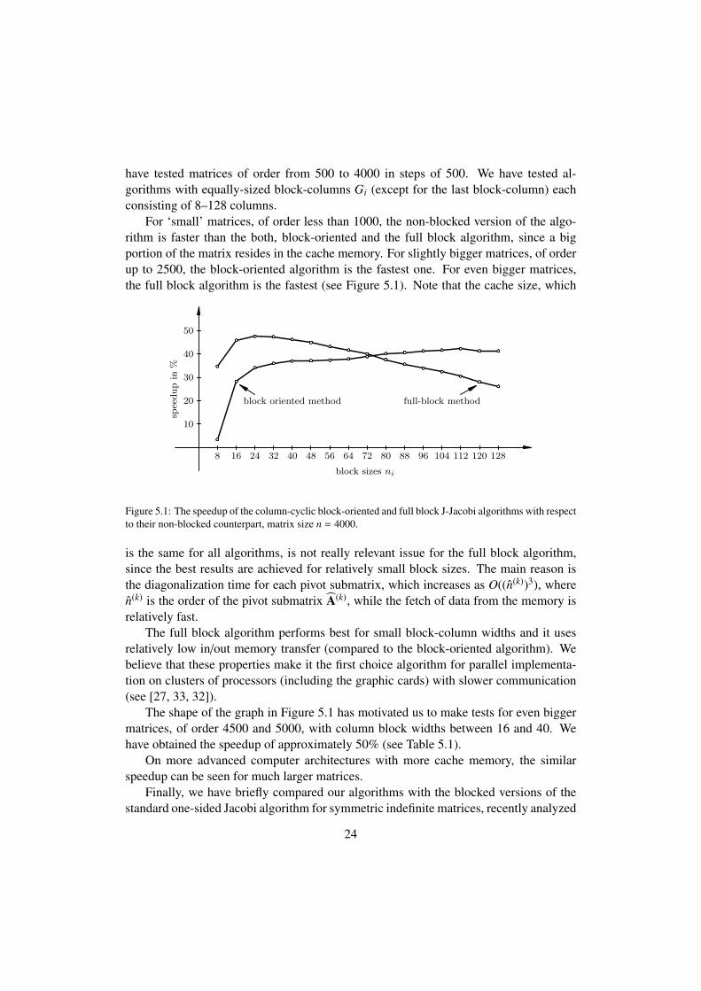
For ‘small’ matrices, of order less than 1000, the non-blocked version of the algo-rithm is faster than the both, block-oriented and the full block algorithm, since a bigportion of the matrix resides in the cache memory. For slightly bigger matrices, of orderup to 2500, the block-oriented algorithm is the fastest one. For even bigger matrices,the full block algorithm is the fastest (see Figure 5.1). Note that the cache size, which

8 16 24 32 40 48 56 64 72 80 88 96 104 112 120 128

10

20

30

40

50

block sizes ni

speedupin

%

block oriented method full-block method

Figure 5.1: The speedup of the column-cyclic block-oriented and full block J-Jacobi algorithms with respectto their non-blocked counterpart, matrix size n = 4000.

is the same for all algorithms, is not really relevant issue for the full block algorithm,since the best results are achieved for relatively small block sizes. The main reason isthe diagonalization time for each pivot submatrix, which increases as O((n(k))3), wheren(k) is the order of the pivot submatrix A(k), while the fetch of data from the memory isrelatively fast.

The full block algorithm performs best for small block-column widths and it usesrelatively low in/out memory transfer (compared to the block-oriented algorithm). Webelieve that these properties make it the first choice algorithm for parallel implementa-tion on clusters of processors (including the graphic cards) with slower communication(see [27, 33, 32]).

The shape of the graph in Figure 5.1 has motivated us to make tests for even biggermatrices, of order 4500 and 5000, with column block widths between 16 and 40. Wehave obtained the speedup of approximately 50% (see Table 5.1).

On more advanced computer architectures with more cache memory, the similarspeedup can be seen for much larger matrices.

Finally, we have briefly compared our algorithms with the blocked versions of thestandard one-sided Jacobi algorithm for symmetric indefinite matrices, recently analyzed

24

Table 5.1: Speedup of the full block algorithm achieved in comparison of the non-block version.

Order n n = 4500 n = 5000Block size ni 16 24 32 40 16 24 32 40Gain (%) 46.16 48.07 47.53 46.88 47.90 50.07 50.52 50.21

in [9]. For computing the complete eigensystem, the J-Jacobi algorithms are signif-icantly faster than the corresponding orthogonal counterparts because they do not useexplicit accumulation of the eingenvector matrix U.

6. Conclusion and future work

In this paper we have considered how to accelerate the accurate eigensolver of Ve-selic [39] for indefinite Hermitian matrices, by modifying it to become the full BLAS 3algorithm. We have considered the most important classes of cyclic pivot strategies, thewavefront and weakly wavefront strategies. We have proved that the full block J-Jacobimethod converges to diagonal form under any weakly wavefront strategy. In addition, wehave shown that under usual assumptions, the full block methods have to be relativelyaccurate. Numerical tests show that for larger matrices, the block algorithms can beeven 50% faster than the non-blocked algorithms. The tests also show that the full blockalgorithms with optimal block sizes are faster than their block-oriented counterparts.

All these results should encourage further research in several directions. There areseveral possibilities how to further accelerate the full block algorithms. In the prepro-cessing part one can try to devise a BLAS 3 modification of the Bunch-Parlett algo-rithm [7] or of the indefinite QR factorization [31]. The modification should try to detecta possible small gap δ0 between the positive and negative part of the spectrum. In theiterative part, one can use ideas from [17, 16] to apply a variant of the fast scaled blocktransformations. The quest for the best pivot strategy is always open. Say, the Mas-carenhas class of cubically convergent quasi-cyclic strategies fits nicely into the initialand basic partitions of A, but should be preceded by faster, probably cyclic strategiesat the beginning of the iteration. Finally, one can try to adapt some of the many tricksadvocated in [14, 15]. The asymptotic quadratic convergence for the block methods stillhas to be proved.

If accuracy is a predominant issue, it is important to devise a criterion, perhaps aftercomputing G (or R), whether to apply the block J-Jacobi method to G or to return to Hand proceed with an orthogonal method, [10] or [9].

25

Acknowledgement

The authors are thankful to Vedran Novakovic for running tests of the algorithms ondifferent machines.

References

[1] C. Ashcraft, R. G. Grimes, J. G. Lewis, Accurate symmetric indefinite linear equation solvers, SIAMJ. Matrix Anal. Appl. 20 (2) (1999) 513–561.

[2] A. W. Bojanczyk, R. Onn, A. O. Steinhardt, Existence of the hyperbolic singular value decomposition,Linear Algebra Appl. 185 (1993) 21–30.

[3] J. R. Bunch, Analysis of the diagonal pivoting method, SIAM J. Numer. Anal. 8 (4) (1971) 656–680.[4] J. R. Bunch, Partial pivoting strategies for symmetric matrices, SIAM J. Numer. Anal. 11 (3) (1974)

521–528.[5] J. R. Bunch, L. C. Kaufman, Some stable methods for calculating inertia and solving symmetric linear

systems, Math. Comp. 31 (137) (1977) 163–179.[6] J. R. Bunch, L. C. Kaufman, B. N. Parlett, Decomposition of a symmetric matrix, Numer. Math. 27 (1)

(1976) 95–109.[7] J. R. Bunch, B. N. Parlett, Direct methods for solving symmetric indefinite systems of linear equations,

SIAM J. Numer. Anal. 8 (4) (1971) 639–655.[8] J. Demmel, K. Veselic, Jacobi’s method is more accurate than QR, SIAM J. Matrix Anal. Appl. 13 (4)

(1992) 1204–1245.[9] F. M. Dopico, P. Koev, J. M. Molera, Implicit standard Jacobi gives high relative accuracy, Numer.

Math. 113 (4) (2009) 519–553.[10] F. M. Dopico, J. M. Molera, J. Moro, An orthogonal high relative accuracy algorithm for the symmet-

ric eigenproblem, SIAM J. Matrix Anal. Appl. 25 (2) (2003) 301–351.[11] Z. Drmac, A global convergence proof of cyclic Jacobi methods with block rotations, SIAM J. Matrix

Anal. Appl. 31 (3) (2009) 1329–1350.[12] Z. Drmac, V. Hari, On quadratic convergence bounds for the J–symmetric Jacobi method, Numer.

Math. 64 (1) (1993) 147–180.[13] Z. Drmac, V. Hari, I. Slapnicar, Advances in Jacobi methods, in: Z. Drmac, V. Hari, L. Sopta, Z. Tutek,

K. Veselic (eds.), Applied Mathematics and Scientific Computing. Proceedings of the 2nd conference,Dubrovnik, Croatia, June 4–9, 2001., Kluwer Academic/Plenum Publishers, New York, 2003, pp. 63–90.

[14] Z. Drmac, K. Veselic, New fast and accurate Jacobi SVD algorithm. I, SIAM J. Matrix Anal. Appl.29 (4) (2008) 1322–1342.

[15] Z. Drmac, K. Veselic, New fast and accurate Jacobi SVD algorithm. II, SIAM J. Matrix Anal. Appl.29 (4) (2008) 1343–1362.

[16] V. Hari, On some new applications of the CS decomposition, in: T. E. Simos, C. Tsitouras (eds.),ICNAAM 2004, International Conference on Numerical Analysis and Applied Mathematics 2004,Chalkis, Greece, September 10–14, 2004, Wiley-VCH, Weinheim, 2004, pp. 161–163.

[17] V. Hari, Accelerating the SVD block–Jacobi method, Computing 75 (2005) 27–53.[18] V. Hari, Quadratic convergence of a special quasi-cyclic Jacobi method, Ann. Univ. Ferrara Sez. VII

Sci. Mat. 53 (2) (2007) 255–269.[19] V. Hari, Convergence to zero of off-diagonal part in block Jacobi-type methods, Preprint, University

of Zagreb, submitted for publication in Numer. Math. (2010).[20] V. Hari, S. Singer, S. Singer, Efficient eigenvalue computation by block modification of the indefinite

one-sided Jacobi algorithm, in: G. P. T. E. Simos, C. Tsitouras (eds.), ICNAAM 2005, InternationalConference on Numerical Analysis and Applied Mathematics 2005, Rhodes, Greece, September 16–20, 2005, Wiley-VCH, Weinheim, 2005, pp. 230–233.

26

[21] V. Hari, S. Singer, S. Singer, Block-oriented J-Jacobi methods for Hermitian matrices, Linear AlgebraAppl. 433 (2010) 1491–1512.

[22] I. C. F. Ipsen, Relative perturbation results for matrix eigenvalues and singular values, in: Acta Nu-merica 1998, Cambridge University Press, Cambridge, 1998, pp. 151–201.

[23] F. T. Luk, H. Park, On parallel Jacobi orderings, SIAM J. Sci. Statist. Comput. 10 (1) (1989) 18–26.[24] F. T. Luk, H. Park, A proof of convergence for two parallel Jacobi SVD algorithms, IEEE Trans.

Comput. C–38 (6) (1989) 806–811.[25] W. F. Mascarenhas, On the convergence of the Jacobi method for arbitrary orderings, SIAM J. Matrix

Anal. Appl. 16 (4) (1995) 1197–1209.[26] J. Matejas, V. Hari, Quadratic convergence estimate of scaled iterates by J-symmetric Jacobi method,

Linear Algebra Appl. 417 (2006) 434–465.[27] V. Novakovic, S. Singer, A GPU-based hyperbolic SVD algorithm, BIT, accepted for publication 51

(2011) 1009–1030.[28] N. H. Rhee, V. Hari, On the global and cubic convergence of a quasi–cyclic Jacobi method, Numer.

Math. 66 (1) (1993) 97–122.[29] A. H. Sameh, On Jacobi and Jacobi–like algorithms for a parallel computer, Math. Comp. 25 (118)

(1971) 579–590.[30] G. Shroff, R. S. Schreiber, On the convergence of the cyclic Jacobi method for parallel block orderings,

SIAM J. Matrix Anal. Appl. 10 (3) (1989) 326–346.[31] S. Singer, Indefinite QR factorization, BIT 46 (1) (2006) 141–161.[32] S. Singer, S. Singer, V. Novakovic, D. Davidovic, K. Bokulic, A. Uscumlic, Three-level parallel J-

Jacobi algorithms for Hermitian matrices, Appl. Math. Comput. 218 (2012) 5704–5725.[33] S. Singer, S. Singer, V. Novakovic, A. Uscumlic, V. Dunjko, Novel modifications of parallel Jacobi

algorithms, Numer. Alg. 59 (2012) 1–27.[34] I. Slapnicar, Accurate symmetric eigenreduction by a Jacobi method, Ph.D. thesis, FernUniversitat–

Gesamthochschule, Hagen (1992).[35] I. Slapnicar, Highly accurate symmetric eigenvalue decomposition and hyperbolic SVD, Linear Al-

gebra Appl. 358 (2003) 387–424.[36] I. Slapnicar, N. Truhar, Relative perturbation theory for hyperbolic singular value problem, Linear

Algebra Appl. 358 (2003) 367–386.[37] N. Truhar, Relative perturbation theory for matrix spectral decompositions, Ph.D. thesis, University

of Zagreb, Zagreb (2000).URL http://www.mathos.hr/~ntruhar/Index/drradnja.ps

[38] A. van der Sluis, Condition numbers and equilibration of matrices, Numer. Math. 14 (1) (1969) 14–23.[39] K. Veselic, A Jacobi eigenreduction algorithm for definite matrix pairs, Numer. Math. 64 (1) (1993)

241–269.[40] K. Veselic, Perturbation theory for the eigenvalues of factorised symmetric matrices, Linear Algebra

Appl. 309 (2000) 85–102.[41] J. H. Wilkinson, Note of the quadratic convergence of the cyclic Jacobi process, Numer. Math. 4 (1)

(1962) 296–300.[42] J. H. Wilkinson, C. Reinsch, Handbook of Automatic Computation II, Linear Algebra, Springer Ver-

lag, Berlin, Heidelberg, New York, 1971.

27