fukaya-seidel categories of hilbert …fukaya-seidel categories of hilbert schemes and parabolic...
TRANSCRIPT

FUKAYA-SEIDEL CATEGORIES OF HILBERT SCHEMES
AND PARABOLIC CATEGORY O
CHEUK YU MAK AND IVAN SMITH
Abstract. We realise Stroppel’s extended arc algebra [51, 13] in the Fukaya-Seidel category of anatural Lefschetz fibration on the generic fiber of the adjoint quotient map on a type A nilpotentslice with two Jordan blocks, and hence obtain a symplectic interpretation of certain parabolic two-block versions of Bernstein-Gelfan’d-Gelfan’d category O. As an application, we give a new geometricconstruction of the spectral sequence from annular to ordinary Khovanov homology. The heart of thepaper is the development of a cylindrical model to compute Fukaya categories of (affine open subsetsof) Hilbert schemes of quasi-projective surfaces, which may be of independent interest.
Contents
1. Introduction 12. The cylindrical Fukaya-Seidel category 53. Properties of the cylindrical Fukaya-Seidel category 254. Comparing Fukaya-Seidel categories 285. Type A geometry 346. The extended symplectic arc algebra 417. More algebra isomorphisms 508. An nc-vector field 559. Formality 6110. Dictionary between Lagrangians and modules 6811. Symplectic annular Khovanov homology 7012. From annular to ordinary Khovanov homology 76Appendix A. Non-formality of standard modules/thimbles 85References 86
1. Introduction
1.1. Summary. This paper has three parts:
• We give a ‘cylindrical’ formulation of the Fukaya category of (an affine open subset of) theHilbert scheme of an affine algebraic surface; (Sections 2-4)• We compute the Fukaya-Seidel category of a natural Lefschetz fibration on the generic fiber
of the adjoint quotient map on the nilpotent / Slodowy slice of Jordan type (n,m− n) arisingfrom its inclusion in the n-th Hilbert scheme of the Milnor fibre of the Am−1-surface singularity,establishing a Morita equivalence to the principal block On,m of BGG parabolic category Oassociated to the partition m = n+ (m− n); (Sections 5-9)• We exploit this equivalence to describe a new semiorthogonal decomposition of perf-On,2n, from
which we derive a geometric construction of the spectral sequence from annular to ordinaryKhovanov homology; (Sections 10-12).
Date: March 12, 2020.Both authors are supported by EPSRC Fellowship EP/N01815X/1.
1
arX
iv:1
907.
0762
4v3
[m
ath.
SG]
10
Mar
202
0

2 CHEUK YU MAK AND IVAN SMITH
1.2. Context. Fix a semisimple complex Lie algebra g. The Bernstein-Gelfan’d-Gelfan’d categoryO is an abelian (Noetherian and Artinian) category of finitely generated g-modules, which plays acentral role in many parts of representation theory. It contains all the highest-weight modules, isclosed under the operations of taking submodules, quotient modules and under tensoring with finite-dimensional modules, and is “minimal” with respect to those properties. Concretely for slm, fixingthe Cartan subalgebra h ⊂ slm of diagonal matrices with respect to a choice of basis, it comprisesthe finitely generated U(slm)-modules which are h-semisimple and which are locally finite for thenilpotent subalgebra n ⊂ slm given by the upper triangular matrices. Given a parabolic subalgebrap ⊂ g containing the Borel n⊕h, there is a parabolic subcategory Op of O consisting of those moduleson which p acts locally finitely. Again for slm, a partition m = m1 + · · ·+mk determines a parabolicp; the extreme cases m = 1 + · · · + 1 and m = m respectively define Op = O and Op = Ofd, thesemisimple category of finite-dimensional slm-modules, so the parabolic subcategories can be viewed asintepolating between these. The central characters decompose Op into blocks and the block containingthe trivial modules is called the principal block Op
0.It is known that for any p ⊂ g, the category Op
0 is equivalent to the category of modules over a finite-dimensional associative algebra; there are algorithmic descriptions of these algebras via quivers withrelations [53], but nonetheless working with them concretely is often rather non-trivial. For parabolicsp ⊂ slm associated to two-block partitions m = n + (m − n), the corresponding category Op
0 = On,mhas several other descriptions: it is Morita equivalent to the category of perverse sheaves on the Grass-mannian Gr(n,m) constructible with respect to the Schubert stratification [10], and the underlying
associative algebra1 Kalgn,m has a diagrammatic description due to Stroppel [51] and Brundan-Stroppel
[13, 12], in which context it is known as the ‘extended arc algebra’. This paper gives a new interpre-tation of these algebras in terms of Fukaya-Seidel categories associated to natural Lefschetz fibrationson the generic fiber of the adjoint quotient map of the nilpotent (Jacobson-Morozov type) slices asso-ciated to nilpotent matrices with two Jordan blocks, and hence a symplectic-geometric construction ofthese particular principal blocks of parabolic category O. This fits into the general dictionary betweensymplectic geometry and aspects of representation theory related to categorification, cf. [26, 11], andsimultaneously extends the symplectic viewpoint on Khovanov homology [47, 1, 2] to a correspondingviewpoint on annular Khovanov homology, complementing recent work of [21, 8].
1.3. Main result. Let π : Am−1 → C be the standard Lefschetz fibration on the Milnor fibre ofthe Am−1-surface singularity, so π is an affine conic fibration with m Lefschetz critical points; thesymplectic topology of this fibration has been extensively studied, see for instance [26, 33]. TheHilbert scheme Hilbn(Am−1) of zero dimensional length n subschemes has a distinguished divisor Dr
of subschemes whose projection under π has length < n, the complement of which is an affine varietyYn,m. (When 2n ≤ m, this space is isomorphic to the generic fibre of the restriction of the adjointquotient map slm → h/W to a transverse slice meeting the nilpotent cone at a matrix with Jordanblocks of size n,m − n, as studied in classical Springer theory [50].) The map π induces a mapπn,m : Yn,m → C which is a Lefschetz fibration in the weak sense that its only critical points areof Lefschetz type (it may, however, have critical points at infinity when n > 1). Nonetheless, thereis a well-defined Fukaya-Seidel A∞-category FS(πn,m), governing the Floer theory of the Lefschetzthimbles associated to any collection of vanishing paths. We write Dπ(C) for the derived category ofC (split-closure of twisted complexes), working over a field K.
Theorem 1.1. If n ≤ m and K has characteristic zero, DπFS(πn,m) is quasi-equivalent to the dg-
category of perfect modules perf-Kalgn,m over Kalg
n,m, hence Morita equivalent to parabolic category On,m.
Remark 1.2. For the extreme case n = m, we have DπFS(πn,m) = Db(K) (see Remark 5.18) and
Kalgn,m := K. When n > m, the map πn,m has no critical point and FS(πn,m) is an empty category;
1 Our Kalgn,m is Km−n
n in [13]. The superscript alg (for algebraic) distinguishes it from a symplectic sibling which is
introduced later in the paper.
FUKAYA-SEIDEL CATEGORIES OF HILBERT SCHEMES AND PARABOLIC CATEGORY O 3
while Kalgn,m is not well-defined. When n = 0, our convention is FS(πn,m) := K and Kalg
n,m := K. Underthis convention, Theorem 1.1 is true for all non-negative integers n,m.
Remark 1.3. The hypothesis on the ground field arises in two places. The first one is a formalitytheorem for the A∞-structure on the symplectic side, which we prove, following [1], via methods of non-commutative algebra which rely on inverting all primes. The second one comes from the constructionof an auxiliary A∞-category FScyl, which is a cylindrical model of the Fukaya-Seidel category, forwhich the definition of the A∞-operations involves dividing out by symmetry groups arising from re-ordering marked points on domains. We work over a characteristic zero field unless stated otherwise.All Lagrangians in the paper are assumed to be orientable and to admit (and be equipped with) spinstructures.
Remark 1.4. It is reasonable to expect that symplectic models for the categories Op, for parabolics pcorresponding to partitions with more parts (or indeed in other simple g), can also be obtained fromthe symplectic geometry of nilpotent slices. In general, however, such slices are not known to be re-interpretable in terms of Hilbert schemes of surfaces, so different techniques would be needed to analysethem. Note that the map πn,m : Yn,m → C is itself obtained from the embedding of Yn,m into a Hilbertscheme; it would be interesting to characterise πn,m intrinsically Lie-theoretically.
There is a well-known ‘tautological correspondence’ between a holomorphic disc in the symmetricproduct of a complex manifold X and a map of a branched cover of the disc to X itself, cf. [17,16, 29, 5] amongst others. Following [29] such correspondences are referred to as ‘cylindrical models’for computing Floer cohomology. Theorem 1.1 uses the embedding Yn,m → Hilbn(Am−1) [31], andthe development of a cylindrical model for computing Fukaya-Seidel categories of Hilbert schemes.Whilst the tautological correspondence has been widely exploited before, the proof nonetheless requiresnumerous technical innovations: we require a model for the whole Fukaya category, our Lagrangiansubmanifolds are not compact and not cylindrical at infinity, and the Hilbert scheme is related to thesymmetric product by a non-trivial crepant resolution. A brief summary of the relevant issues is givenin Section 2.1 (our treatment requires only classical transversality theory, but an appeal to virtualperturbation theory would not bypass many of the difficulties).
1.4. Consequences. As commented previously, Kalgn,m is Morita equivalent to a category of perverse
sheaves on the Grassmannian Gr(m,n). From the (Schubert-compatible) isomorphism Gr(n,m) =Gr(m− n,m), one obtains a geometrically non-trivial:
Corollary 1.5. DπFS(πn,m) is quasi-equivalent to DπFS(πm−n,m).
Note that the categories appearing in Corollary 1.5 are associated to Hilbert schemes of n re-spectively m − n points, so take place in symplectic manifolds of different dimension. For another
non-trivial symmetry, the identity Kalgn,m∼= (Kalg
n,m)op of the arc algebra with its opposite – which hasan easy diagrammatic proof – is non-trivial on the geometric side, because of the non-trivial boundaryconditions and ‘wrapping’ involved in setting up a Fukaya-Seidel category (cf. Section 9.2).
The Fukaya-Seidel category of any Lefschetz fibration has a full exceptional collection. Additivityof Hochschild homology under semi-orthogonal decomposition [28] immediately yields:
Corollary 1.6. The Hochschild homology of the extended arc algebra HH∗(Kalgn,m) vanishes in degree
∗ 6= 0, and in degree zero is free of rank(mn
).
The Corollary was previously established by Beliakova et al [8] by an ingenious and involved alge-braic argument involving a ‘quantum deformation’ of the Hochschild complex.
Underlying and extending Theorem 1.1, and the previous Corollaries, there is a rich dictionarybetween objects in the representation theory and in the symplectic geometry, which is useful in bothdirections. The blocks of parabolic category O are renowned instances of highest-weight categories, i.e.ones with a full exceptional collection where the exceptional objects generate rather than just split-generate. A key point in the proof of Theorem 1.1 is that the endomorphism algebra of the collection

4 CHEUK YU MAK AND IVAN SMITH
of Lagrangian submanifolds associated to projective modules is formal. Crucially, the ‘projective’Lagrangians are predicted by the diagrammatic combinatorics on the algebra side; away from Milnorfibres of surface singularities, they have no obvious counterpart for Hilbert schemes of general Lefschetzfibrations on quasi-projective surfaces.
Remark 1.7. In contrast to a number of recent formality results which hold (for instance) for degreereasons, the formality of the symplectic extended arc algebra holds for non-trivial geometric reasons,and is established, following [1], by building a non-commutative vector field b ∈ HH1(FS(πn,m))counting certain holomorphic curves with prescribed behaviour at infinity. The endomorphism algebraof the Lefschetz thimbles is in general not formal (cf. Appendix A), and it seems hard to prove Theorem1.1 by directly comparing the A∞-algebras associated to distinguished bases of exceptional objects.
In the other direction, the geometry gives rise rather directly to the following:
Theorem 1.8 (see Theorem 11.9). There is a semi-orthogonal decomposition perf-Kalgn,m = 〈An, . . . , A0〉
where Aj is quasi-equivalent to perf-(Kalgj,n ⊗K
algn−j,m−n) for all j = 0, . . . , n.
The equivalence of Theorem 1.8 does not send tensor products of projectives to projectives, whichmay make it less transparent from the viewpoint of the extended arc algebras themselves.
1.5. Invariants of braids. The braid group Brm acts by symplectomorphisms on Yn,m; a braid β
defines a symplectomorphism φ(n)β and a corresponding bimodule P
(n)β over the Fukaya-Seidel category
DπFS(πn,m). The Hochschild homology HH∗(P(n)β ) is an algebraic analogue of the natural symplectic
invariant HF ∗(φ(n)β ) given by taking fixed-point Floer cohomology2. We define the symplectic annular
Khovanov homology of β ∈ Brm by
AKhsymp(β) := ⊕mj=0HH∗(P(j)β ).
This is by definition an invariant of the braid. Recall from [47] that there is a distinguished closedexact Lagrangian submanifold L℘ ⊂ Yn,2n with the property that
Khsymp(κ(β)) := HF ∗(L℘, φ(n)β (L℘))
is an invariant of the link closure κ(β) of β ∈ Brn, known as ‘symplectic Khovanov cohomology’. Thiswas introduced in [47] as a singly graded sibling to combinatorial Khovanov homology; working overa characteristic zero field K, the isomorphism Kh(κ(β)) ∼= Khsymp(κ(β)) of Z-graded3 vector spaceswas established in [1, 2].
Theorem 1.9. There is a spectral sequence AKhsymp(β)⇒ Khsymp(κ(β)) from the symplectic annularKhovanov homology of β to the symplectic Khovanov cohomology of the link closure κ(β) of β.
Annular Khovanov homology was introduced by Asaeda, Przytycki and Sikora in [4], via a di-agrammatic calculus for links in a solid torus. Roberts [39] showed there is a spectral sequenceAKh(β) ⇒ Kh(κ(β)), but the fact that AKh(β) splits into summands which can be identified withHochschild homology groups is non-trivial; this was conjectured by Auroux, Grigsby and Wehrli [6]and proven very recently by Beliakova, Putyra and Wehrli [8]. By contrast, if one had defined the an-nular Khovanov invariant as such a direct sum of Hochschild homologies, the existence of the spectral
sequence would seem rather mysterious: the bimodules P(j)β over the categories FS(πj,m) do not in
themselves have enough information to determine the differentials in the spectral sequence (which donot preserve the decomposition by j). Theorem 1.9 gives a geometric explanation for the existence of a
2There are numerous results relating fixed-point Floer cohomology and Hochshild homology, see e.g. [43], which forinstance show that the two invariants co-incide when n = 1. When n > 1, since πn,m has critical points at infinity, theestablished results do not apply in our case; for simplicity we take our basic invariant of a braid to be the bimodule.
3In this paper we will not discuss the grading; the methods of [1] give rise to a second grading by elements of K, whichis conjecturally integral, Markov-invariant and lifts the Z-graded equivalence to a bigraded equivalence.

FUKAYA-SEIDEL CATEGORIES OF HILBERT SCHEMES AND PARABOLIC CATEGORY O 5
spectral sequence from a direct sum of Hochschild homologies to (symplectic) Khovanov cohomology;the crucial input is the semi-orthogonal decomposition from Theorem 1.8. We remark that there is ananalogous spectral sequence from knot Floer homology, viewed as Hochschild homology of a suitablebimodule via [30], to Heegaard Floer homology; it would be interesting to see if that can be derivedfollowing the methods of this paper.
1.6. Outline of the paper. Let πE : E → C be a Lefschetz fibration on a quasi-projective surface.
The map πE defines a map π[n]E : Hilbn(E) → C, by taking the map induced from the sum of copies
of πE on the product En. The map π[n]E is a Lefschetz fibration when restricted to the affine open
subvariety of the Hilbert scheme Hilbn(E) comprising subschemes whose projection to C has lengthn. Section 2 develops a cylindrical model FScyl for the Fukaya(-Seidel) category of this associatedLefschetz fibration; section 3 establishes some basic properties of FScyl analogous to the usual Fukaya(-Seidel) category; section 4 relates the cylindrical model to the usual model FS, yielding in general anembedding FS → FScyl; and section 5 applies this framework to type A Milnor fibres. Sections 6-7construct a symplectic version of the extended arc algebra, which is a priori an A∞-algebra, and provethat its cohomology agrees with its combinatorial sibling; sections 8-9 then prove the A∞-structureis actually formal in characteristic zero. Section 10 illustrates the dictionary between natural objectsin the representation theory of the extended arc algebras and their geometric counterparts. Sections11 and 12 introduce symplectic annular Khovanov homology, and relate this to ordinary Khovanovhomology via a particular semiorthogonal decomposition of the Fukaya-Seidel category associated tothe (n, 2n)-nilpotent slice (associated to a nilpotent with Jordan blocks of size (n, n)). The Appendixshows that the A∞-endomorphism algebra of the thimbles in the Fukaya-Seidel category is in generalnot formal; this underscores the important contribution of the relationship to representation theory,which picks out a different set of generators for the category (as studied in sections 5-9) which do haveformal endomorphism algebra.
Acknowledgements. The authors are grateful to Mohammed Abouzaid, Robert Lipshitz, JacobRasmussen, Catharina Stroppel and Filip Zivanovic for many helpful conversations. We thank theanonymous referee for their numerous helpful comments and corrections.
2. The cylindrical Fukaya-Seidel category
2.1. Overview. The aim of this section is to define, given a Lefschetz fibration πE on a complexsurface E equipped with an exact symplectic structure (that satisfies some mild additional hypothesis,see Section 2.2.4) and a positive integer n, an A∞ category FScyl,n(πE), which we call the n-foldcylindrical Fukaya-Seidel category. Objects in this category are, roughly speaking, unordered n-tuplesof pairwise disjoint exact Lagrangians L = L1, . . . , Ln, with Li ⊂ E. The product of the Li definesa Lagrangian (which descends to one) in Symn(E), which can be lifted to a Lagrangian Sym(L) inHilbn(E).
Let π[n]E : Hilbn(E)→ C be the map induced from the sum of n copies of πE . There is a divisor Dr
of Hilbn(E) such that YE := Hilbn(E) \Dr admits an exact symplectic structure, and such that
πYE := π[n]E |YE : YE → C(2.1)
is a Lefschetz fibration in the weak sense that all the critical points of πYE are of Lefschetz type4.Every Lefschetz thimble of πYE is given by Sym(L) for some L. If E is the Am−1-Milnor fiber and πE isthe conic fibration with m critical points, then YE and πYE coincide with Yn,m and πn,m, respectively.
The A∞ structure of FScyl,n(πE) is carefully defined so that it has the property that the categoryof Lefschetz thimbles of πYE embeds into FScyl,n(πE) as a full subcategory, where on the object level,it is given by Sym(L) 7→ L. This reduces calculations in the Fukaya-Seidel category of πYE to more
accessible calculations in FScyl,n(πE), which involve holomorphic curve counts in E itself.
4There may be critical points at infinity, so this is not a symplectic Lefschetz fibration in the usual sense.

6 CHEUK YU MAK AND IVAN SMITH
Ideally, we would like to have a choice of perturbation scheme such that there is a bijective corre-spondence between (perturbed)-holomorphic polygons u : S → YE contributing to the A∞ structureof FS(πYE ) and pairs (πΣ, v) such that πΣ : Σ → S is an n-fold branched covering and v : Σ → Eis a solution to a (perturbed)-holomorphic equation. In this case, if we define the A∞ structure ofFScyl,n(πE) as a signed rigid count of the pairs (πΣ, v), then it would be tautological that the A∞categories FS(πYE ) and FScyl,n(πE) would be equivalent. Problems arise when one implements thisidea in practice:
• The domain-dependent almost complex structure on E has to be complex (and hence inducean almost complex structure on Hilbn(E)) to have any hope of a bijective correspondencebetween u and (πΣ, v), which puts some restrictions on the perturbation scheme;• Hamiltonian perturbations in Hilbn(E) that are simultaneously induced from Hamiltonian
perturbations in E and which preserve Dr are not general enough to achieve transversality;strictly speaking, there is no perturbation scheme that can allow us to define the A∞ structureof FScyl,n(πE) by merely counting (πΣ, v);• We need to include some L for which Sym(L) is not cylindrical in YE (e.g. to obtain formal A∞
Floer cochain algebras in the setting of Theorem 1.1), so compactness of the moduli involvedhas to be carefully addressed.
Our main contribution to the construction of FScyl,n(πE) is to overcome the above difficulties,roughly as follows:
• Instead of using moduli of polygons Rd+1, we use moduli of polygons with ordered interiormarked points Rd+1,h to define the A∞ structure. The interior marked points keep track ofthe branch points of πΣ : Σ→ S, and the domain-dependent almost complex structure is onlyrequired to be integrable near the interior marked points. This gives us more flexibility forthe perturbation scheme and at the same time partially recovers the bijective correspondencebetween u and (πΣ, v).• Whilst the A∞ structure of FScyl,n(πE) is defined by counting certain solutions u mapping
to Hilbn(E) \ Dr, rather than pairs (πΣ, v), our set up is sufficiently flexible that the Floerdifferential and product can be computed by counting solutions (πΣ, v).• To achieve compactness, we need to avoid that solutions in Hilbn(E)\Dr escape to the vertical
boundary, horizontal boundary or Dr. No escape along the vertical boundary is achieved bymodifying Seidel’s ingenious set-up in [46]; one takes the base of the Lefschetz fibration tobe the upper half-plane, and uses hyperbolic isometries to gauge back perturbed holomorphiccurves to actual holomorphic curves. No escape along the horizontal boundary and into Dr
are each achieved by positivity of intersection, which relies on a delicate choice of Hamiltonianperturbation scheme and some particular geometric features of Dr. Familiarity with [46] maybe helpful.
2.2. Definitions and the setup.
2.2.1. Domain moduli. Let Rd+1,h be the moduli space of discs with d+ 1 punctures on the boundaryand h ordered and pairwise distinct interior marked points. Let Sd+1,h be the universal family ofRd+1,h. We fix a distinguished puncture ξ0 for the elements in Rd+1,h consistently, and order theremaining punctures ξ1, . . . , ξd counter-clockwise along the boundary. For S ∈ Rd+1,h, we denote theordered interior marked points by ξ1
+, . . . ξh+ and we use ∂jS to denote the boundary component of S
between ξj and ξj+1 for j = 0, . . . , d (ξd+1 is understood as ξ0). We use mk(S) to denote the set ofinterior marked points of S.
The moduli space Rd+1,h can be compactified to the moduli of stable discs Rd+1,h. The latter
moduli is used to define bulk deformation in [20], [48], to which readers are referred for the details of
its construction. We denote the universal family over Rd+1,hby Sd+1,h
.

FUKAYA-SEIDEL CATEGORIES OF HILBERT SCHEMES AND PARABOLIC CATEGORY O 7
2.2.2. Strip-like ends and marked-points neighborhoods. For each Rd+1,h, we make a choice of strip-like ends ε = ε0, . . . , εd for elements in Rd+1,h such that ξ0 is an output and ξj is an input forj = 1, . . . , d. Thus, for each S ∈ Rd+1,h, we have holomorphic embeddings varying smoothly respectto S
ε0 : R≤0 × [0, 1]→ Sε1, . . . εd : R≥0 × [0, 1]→ Slims→±∞ ε
j(s, ·) = ξj
(εj)−1(∂S) = (s, t) : t = 0, 1.
We denote ∪S∈Rd+1,hIm(εj) in Sd+1,h by Nd+1,hεj .
Furthermore, we choose a ‘marked-points neighborhood’ ν(mk(S)) for each S ∈ Rd+1,h, which is a(possibly disconnected) open subset of S containing mk(S), such that
Nd+1,hmk := ∪S∈Rd+1,hν(mk(S))(2.2)
is a smooth submanifold (with boundary) in Sd+1,h. We require that Nd+1,hmk ∩Nd+1,h
εj = ∅ for all j.
We fix a choice of cylindrical ends for the interior marked points of S ∈ Rd+1,h, and for the interiormarked points for the elements in the moduli of spheres with ordered marked points. Given that
choice, one obtains a smooth structure on Rd+1,h(see [48, Section 4], [40, Section (9g)]).
A choice of strip-like ends for all elements of Rd+1,h, for all d and h, is called consistent if it extends
to a choice of strip-like ends (smooth up to the boundary) for all elements in Rd+1,h. A choice of
marked-points neighborhoods for all elements of Rd+1,h, for all d and h, is called consistent if the
closure of their union, denoted by Nd+1,hmk , is a smooth submanifold with boundary and corners in
Sd+1,h. We fix such a consistent choice of strip-like ends and marked-points neighborhoods.
Remark 2.1. Note that mk(S) ⊂ ν(mk(S)) for all S ∈ Rd+1,h implies that if S ∈ Rd+1,hhas a stable
sphere component Q, then Q ⊂ ν(mk(S)).
2.2.3. An isometry group. Let Gaff be the group of orientation preserving affine transformations ofthe real line and gaff be its Lie algebra. Let H be the closed upper half-plane, whose interior H is
equipped with the hyperbolic area form ωH = dre(w)∧dim(w)im(w)2 and primitive θH = −dc(log(im(w))). We
write ∂∞H := H \H.The Gaff -action on the real line extends to H and we have Lie algebra homomorphism
gaff → C∞(H, TH)(2.3)
which sends γ ∈ gaff to a Hamiltonian vector field Xγ . We define
(2.4) Hγ := θH(Xγ)
which is a Hamiltonian on H generating Xγ .
2.2.4. Target space. Our setup is modified from [46]. Let (Ee, JEe) be a complex surface with boundaryand let
πEe : Ee :→ H(2.5)
be a proper Lefschetz fibration such that ∂Ee = π−1Ee
(∂H). Let ωE be a symplectic form on E :=
Ee \ ∂Ee which tames JE := JEe |E and makes
πE := πEe |E → H(2.6)
into a symplectic Lefschetz fibration.Let DE be a smooth and reduced (but possibly disconnected) divisor of Ee. Let E := E \ DE ,
JE := JEe |E , ωE := ωE |E and πE := πE |E . We assume that there is a primitive θE for ωE on E (so,in particular, it implies that πEe |DE is surjective).

8 CHEUK YU MAK AND IVAN SMITH
We assume that there is a contractible compact subset CH ⊂ H such that πE |π−1
E(H\CH) is sym-
plectically locally trivial. It means that for all x ∈ π−1E
(H \ CH)
(1) x is a regular point of πE , and
(2) the horizontal distribution T hxE := (T vxE)⊥ω
E is integrable in a neighborhood of x, and(3) ωE |ThxE = (πE)∗ωH |ThxE
We also require that for x ∈ DE ∩ π−1E
(H \ CH), we have T hxE = TxDE .
If we pick a point ∗ ∈ H \ CH and define (F, ωF , θF ) := (π−1E (∗), ωE |π−1
E (∗), θE |π−1E (∗)), then the
conditions above imply that for every z ∈ H \ CH, there is an open neighborhood U of z, anda symplectomorphism (π−1
E (U), ωE) → (U × F, ωH |U + ωF ) compatible with the projection to U .
Therefore, there is a natural way to extend the symplectic form ωE to ωEe on Ee.Let J (E) be the space of ωE-tamed almost complex structures J on E such that
J = JE outside a compact subset in E(2.7)
πE is (J, jH)-holomorphic.(2.8)
Condition (2.7) implies that every J ∈ J (E) can be smoothly extended to an ωEe-tamed almost
complex structure Je on Ee, and we assume that
every Je-holomorphic map CP1 → Ee has positive algebraic intersection number with DE .(2.9)
We also assume that c1(E) = 0 and a trivialization of the canonical bundle is chosen.For γ ∈ gaff , let
Hγ(H) :=H ∈ C∞(H,R)|H is a constant in a neighborhood of CH,(2.10)
and H = Hγ outside a compact subset of HHγ(E) :=H ∈ C∞(E,R)|H = π∗EH
′ for some H ′ ∈ Hγ(H)(2.11)
Then for H ∈ Hγ(H), we have
XH |CH = 0 and XH = XHγ outside a compact set.(2.12)
Since πE is symplectically locally trivial outside π−1E (CH), for H ∈ Hγ(E), XH is uniquely determined
by the property that
(πE)∗(XH |x) = XH′ |πE(x)(2.13)
for all x ∈ E. If we extend XH to a smooth vector field on E, we also have
XH |x ∈ TxDE for all x ∈ DE(2.14)
Next, we consider the class L of properly embedded, oriented and spin Lagrangian submanifoldsL ⊂ E such that
πE |L is proper and ∂L = ∅(2.15)
there is a compact subset CL ⊂ H such that πE(L) \ CL is either empty or is a properly(2.16)
embedded arc γL in H, and if πE(L) \ CL 6= ∅ then we denote the point γL \ γL by λL ∈ R,
where γL is the closure of γL in HL is exact with respect to θE .(2.17)
Note that, if A = atdt ∈ Ω1([0, 1], gaff)H = (Ht)t∈[0,1] such that Ht ∈ Hat(E)
(2.18)

FUKAYA-SEIDEL CATEGORIES OF HILBERT SCHEMES AND PARABOLIC CATEGORY O 9
and φH is the associated Hamiltonian diffeomorphism (which is well-defined everywhere becauseφH |π−1
E (CH) is the identity), then φ−1H (L) ∈ L and λφ−1
H (L) = g−1A λL, where gA ∈ Gaff is the paral-
lel transport from 0 to 1 with respect to A (see Figure 2.1).
x x x x
λL
π
φ
E
-1H
(L))(
(L)λ
πEφ-1
H(L)
Figure 2.1. An example of πE(L) (black) and πE(φ−1H (L)) (red); crosses are critical values.
Finally, we consider the set Lcyl,n of (unordered) n-tuples of Lagrangians L = L1, . . . , Ln suchthat
Lk ∈ L for k = 1, . . . , n(2.19)
there are pairwise disjoint contractible open sets ULk in H such that(2.20)
πE(Lk) ⊂ ULk and ULk ∩ ∂H is either empty or contractible
In particular, (2.20) implies that the Lk are pairwise disjoint. We define
Sym(L) := qSn(L1 × · · · × Ln) ⊂ Confn(E) ⊂ Symn(E)(2.21)
Sym(UL) := qSn,H(UL1 × . . . ULn) ⊂ Symn(H)(2.22)
λL := [minkλLk,max
kλLk] ⊂ R(2.23)
where qSn : En → Symn(E) and qSn,H : (H)n → Symn(H) are the quotient maps by the symmetricgroup. When λL = ∅ (i.e. when πE(Lk) is compact for all k = 1, . . . , n), we define λL := 0 so λL is
a non-empty closed interval for all L ∈ Lcyl,n.
2.2.5. Hilbert scheme of points. Let Hilbn(E) be the Hilbert scheme of zero dimensional length nsubschemes on E, defined with respect to the complex structure JE on E. We denote the Hilbert-Chow divisor by DHC and the relative Hilbert scheme with respect to πE by Dr, i.e. this is thedivisor of subschemes whose projection under πE has length < n. (We will sometimes write YEfor the complement Hilbn(E)\Dr when the particular value of n is implicit or plays no role.) LetπHC : Hilbn(E) → Symn(E) be the contraction of DHC and Symn(πE) : Symn(E) → Symn(H) bethe natural map induced by πE . Let ∆H ⊂ Symn(H) be the big diagonal (i.e. all unordered tuplesq1, . . . , qn of points in H such that qi = qj for some i 6= j).
Lemma 2.2. (Symn(πE) πHC)−1(∆H) = DHC ∪Dr.
Proof. It is clear that Symn(πE) πHC(DHC ∪ Dr) ⊂ ∆H . For the converse, if the support ofz ∈ Hilbn(E)∩ (Symn(πE) πHC)−1(∆H) is a union of distinct n points, then z ∈ Dr. If the supportconsists of k < n points instead, then z ∈ DHC .
Note that Hilbn(E) \ DHC = Confn(E), and we have a trivialization of the canonical bundle ofConfn(E) induced by that of E.
Lemma 2.3. The trivialization of the canonical bundle of Confn(E) extends smoothly to a trivializa-tion of the canonical bundle of Hilbn(E).
Proof. It follows from the fact that πHC is a crepant resolution of Symn(E).
We equip Confn(E) with the product symplectic form ωConfn(E) from (E,ωE). This is smooth, butcannot be smoothly extended to a 2-form on Hilbn(E).

10 CHEUK YU MAK AND IVAN SMITH
Lemma 2.4. For every open neighborhood U ⊂ Hilbn(E) of DHC , there is a symplectic form onHilbn(E) which tames the complex structure, and coincides with ωConfn(E) outside U .
Proof. This follows essentially from [52], see also [36, 37] in the Kahler case. Let DeHC be the Hilbert-
Chow divisor of Hilbn(Ee). Let U, V ⊂ Hilbn(Ee) be an open neighborhoods of DeHC such that
U contains the closure of V . In [52], Voisin constructed two smooth closed two-forms χ and Ψ
on Hilbn(Ee) such that for some λ0 > 0 and for all λ ∈ (0, λ0), χ + λΨ is a symplectic form on
Hilbn(Ee) that tames the complex structure. Moreover, χ|Hilbn(Ee)\V = ωConfn(Ee)|Confn(Ee)\V and
Ψ|Hilbn(Ee)\DeHC
= dΘ for some Θ ∈ Ω1(Hilbn(Ee) \DeHC).
Let ρ : Hilbn(Ee) → [0, 1] be a cut off function such that ρ|V = 1 and ρ = 0 outside U . Then(χ+ λd(ρΘ))|Hilbn(Ee)\U = ωConfn(Ee)|Confn(Ee)\U and (χ+ λd(ρΘ))|V = (χ+ λΨ)|V .
Since χ is non-degenerate and tames the complex structure outside V , and being non-degnerateand taming are both open conditions, for sufficiently small λ > 0, we know that χ + λd(ρΘ) is asymplectic form which tames the complex structure outside V . Moreover, this is also true inside Vbecause χ+ λd(ρΘ) = χ+ λΨ inside V . Therefore, we can restrict this symplectic form to Hilbn(E)to get the result.
Lemma 2.5. If C is the image of a non-constant rational curve in Hilbn(E), then [C] · [Dr] > 0.
Proof. From Lemma 2.4, one sees that the symplectic form on Hilbn(E) is Poincare dual to the relativecycle −ε[DHC ] for some ε > 0 (recall that ωE is exact). It is proved in [1, Lemma 5.4] that [Dr] is apositive multiple of −[DHC ] so [C] · [Dr] > 0 follows from positivity of the symplectic area of C.
Let Dr = Dr ∩ Confn(E). For J ∈ J (E), we define J [n] to be the almost complex structure on
Confn(E) decended from the product almost complex structure Jn on En. Note that J [n] is ωConfn(E)-
tamed and when J = JE , J [n] extends smoothly to Hilbn(E). We define the following space of almostcomplex structures on Confn(E):
J n(E) :=J |J = (J ′)[n] for some J ′ ∈ J (E)(2.24)
For H ∈ C∞(E,R), we define H [n] ∈ C∞(Confn(E),R) to be
H [n](z) :=n∑i=1
H(zi)(2.25)
for z = z1, . . . , zn ∈ Confn(E). For γ ∈ gaff , let
Hn,preγ (E) :=H ∈ C∞(Confn(E),R)|H = (H ′)[n] for some H ′ ∈ Hγ(E)(2.26)
Hnγ (E) :=H ∈ C∞(Confn(E),R)|H = H ′ outside a compact subset of(2.27)
Confn(E) \Dr , for some H ′ ∈ Hn,preγ (E)Note that, if
A = atdt ∈ Ω1([0, 1], gaff)
H = (Ht)t∈[0,1] such that Ht = (H ′t)[n] ∈ Hn,preat (E) for H ′t ∈ Hat(E)
(2.28)
then φH is a well-defined Hamiltonian diffeomorphism of Confn(E) and the Hamiltonian vector fieldXHt satisfies
XHt |p ∈ TpDr(2.29)
for all p ∈ Dr and for all t ∈ [0, 1]. It implies that φH(Dr) = Dr . Moreover, we have φ−1H (Sym(L)) =
Sym(φ−1H′ (L)) ∈ Symn(L) and
λφ−1H′ (L) = g−1
A λL.(2.30)
FUKAYA-SEIDEL CATEGORIES OF HILBERT SCHEMES AND PARABOLIC CATEGORY O 11
As a result, if H = (Ht)t∈[0,1] and Ht ∈ Hnat(E) for all t, the associated Hamiltonian vector fieldsatisfies (2.29) and φH is also a well-defined Hamiltonian diffeomorphism of Confn(E). Moreover,φ−1H (Sym(L)) = Sym(L′) outside a compact set of Confn(E) \Dr for some L′ ∈ Lcyl,n. Therefore, we
can define λφ−1H (Sym(L)) = λL′ .
Remark 2.6. We introduce both Hn,preγ (E) and Hnγ (E) because, on the one hand, Hnγ (E) gives us
more freedom to achieve transversality, but on the other, working with Hn,preγ (E) simplifies explicitcomputations for cases that transversality can be achieved within that more restricted class.
2.2.6. Floer cochains. Let Gaff([0, 1]) := C∞([0, 1], Gaff) which is weakly contractible. Let Iaff be theset of non-empty closed intervals in R. Let
Caff([0, 1]) := (λ0, λ1) ∈ I2aff |λ0 > λ1(2.31)
where the strict inequality means minλ0 > maxλ1. For each Φ ∈ Gaff([0, 1]) and (λ0, λ1) ∈ I2aff , we
define
Φ∗(λ0, λ1) := (Φ∗(0aff),Φ0(λ0),Φ1(λ1)) ∈ Ω1([0, 1], gaff)× I2aff(2.32)
where 0aff is the trivial connection, Φ∗(0aff) is the gauge transformation by Φ and Φi := Φ(i) fori = 0, 1. We define
Paff([0, 1]) := Φ∗(λ0, λ1)|(λ0, λ1) ∈ Caff([0, 1]).(2.33)
Note that, if (A, λ0, λ1) ∈ Paff([0, 1]), then by (2.31) and (2.32), we have
g−1A λ1 < λ0.(2.34)
Lemma 2.7 (cf. Section (2a) of [46]). Paff([0, 1]) is non-empty and weakly contractible. The projection
Paff([0, 1])→ I2aff(2.35)
is a surjective weak fibration. Therefore, the fibers of (2.35) are also weakly contractible.
Proof. Since Φ∗(λ0, λ1) = Φ′∗(λ′0, λ′1) if and only if Φ (Φ′)−1 is a constant and λj = Φ (Φ′)−1(λj) for
j = 0, 1, Paff([0, 1]) can be identified with Gaff([0, 1]) ×GaffCaff([0, 1]). That implies that Paff([0, 1]) is
non-empty and weakly contractible.On the other hand, given λ0, λ1 ∈ Iaff , there exists g ∈ Gaff such that g−1λ1 < λ0. Moreover, there
exists Φ ∈ Gaff([0, 1]) such that for A := Φ∗(0aff), we have gA = g. It follows that (2.35) is surjective.We leave to readers to check that (2.35) is a weak fibration (cf. [46, Section (2a)]).
We denote the fiber of (2.35) at (λ0, λ1) by Aaff([0, 1], λ0, λ1).
Definition 2.8. For L0 = L0,knk=1 and L1 = L1,knk=1 in Lcyl,n, a perturbation pair is a pair(AL0,L1
, HL0,L1) such that
AL0,L1= aL0,L1,tdt ∈ Aaff([0, 1], λL0
, λL1)
HL0,L1= (HL0,L1,t)t∈[0,1], HL0,L1,t ∈ H
naL0,L1,t
(E)(2.36)
and
φ−1HL0,L1
(Sym(L1)) t Sym(L0).(2.37)
Lemma 2.9. For any L0, L1 ∈ Lcyl,n, the set of perturbation pairs is non-empty.
Proof. For any choice of (AL0,L1, HL0,L1
) satisfying (2.36), by (2.30) and (2.34), we have
λφ−1HL0,L1
(Sym(L1)) < λL0(2.38)
so the transversality condition (2.37) is satisfied outside a compact subset. By definition (2.27), weare free to perturb HL0,L1
inside a compact subset, so the result follows (cf. Remark 2.6).

12 CHEUK YU MAK AND IVAN SMITH
Let X (HL0,L1, L0, L1) = φ−1
HL0,L1(Sym(L1)) t Sym(L0) which is identified with the set of XHL0,L1
-
chords from Sym(L0) to Sym(L1). By (2.29) and the fact that Sym(L) ⊂ Confn(E) \ Dr for everyL ∈ Lcyl,n, we know that
the XHL0,L1-chords from Sym(L0) to Sym(L1) are disjoint from Dr .(2.39)
Example 2.10. If (2.37) can be achieved by HL0,L1,t = (H ′L0,L1,t)[n] ∈ Hn,preaL0,L1,t
(E), then the set
X (HL0,L1, L0, L1) can be identified with the set of unordered n-tuples x = (x1, . . . , xn) such that xk ∈
φ−1H′L0,L1
(L1,bk) t L0,ak , where ak : k = 1, . . . , n = bk : k = 1, . . . , n = 1, . . . , n (see Figure 2.2).
x x x x
Figure 2.2. Lagrangian tuples πE(L0) (black) and πE(φ−1H′L0,L1
(L1)) (red) for H ′L0,L1∈
Hγ(E)
Given L0, L1 ∈ Lcyl,n, a perturbation pair (AL0,L1, HL0,L1
) and a smooth family J = (Jt)t∈[0,1], Jt ∈J n(E), we define the Floer cochains (as a vector space over a chosen coefficient field of characteristiczero5) by
CF (L0, L1) := ⊕x∈X (HL0,L1,L0,L1)ox(2.40)
where ox is the orientation line at x. In this case, we call (AL0,L1, HL0,L1
, J) a Floer cochain datum
for L0, L1 ∈ Lcyl,n.For a fixed choice of grading functions η0,k on L0,k and η1,k on L1,k, for k = 1, . . . , n, Lemma 2.3
implies that the product∏k ηi,k descends to a grading function on Sym(Li), and we use that to grade
X (HL0,L1, L0, L1).
Example 2.11. In the situation of Example 2.10, the grading of x = (x1, . . . , xn) is
|x| =n∑j=1
|xj |(2.41)
where |xj | is the Floer grading of xj in E.
2.2.7. Floer data. We define the following group of gauge transformations:
Gaff(Sd+1,h) := Φ ∈ C∞(Sd+1,h
, Gaff) :Φ|Nd+1,hmk
= idGaffand Φ(εj(s, t)) is independent of(2.42)
both s and S ∈ Rd+1,h.
where Nd+1,hmk is defined in Section 2.2.2.
Lemma 2.12. Gaff(Sd+1,h) is weakly contractible.
Proof. Recalling that Gaff is contractible and Nd+1,hmk is a codimension 0 smooth submanifold of Sd+1,h
with boundary and corner. The result follows from the weak fibration
Gaff(Sd+1,h)→ C∞(Sd+1,h
, Gaff)→ C∞(Nd+1,hmk , Gaff)×
d∏j=0
C∞(εj(0, [0, 1]), Gaff)(2.43)
5Recall that to work in characteristic zero requires that we fix spin structures on the Lagrangians; in the main examplesstudied later in the paper, the Lagrangians are products (S2)j × (R2)k for j, k ≥ 0 and admit unique spin structures.

FUKAYA-SEIDEL CATEGORIES OF HILBERT SCHEMES AND PARABOLIC CATEGORY O 13
Similarly to (2.31), we define
Caff(Sd+1,h) := (λ0, . . . , λd) ∈ Id+1
aff |λ0 > λ1 > · · · > λd.(2.44)
Consider a trivial Gaff -bundle over Sd+1,hwith fiber R and equip it with the trivial connection 0aff .
For Φ ∈ Gaff(Sd+1,h) and λ ∈ C∞(∂Sd+1,h
, Iaff), we define
Φ∗λ :=(Φ∗0aff ,Φ λ) ∈ Ω1(Sd+1,h, gaff)× C∞(∂Sd+1,h
, Iaff)(2.45)
Paff(Sd+1,h) :=Φ∗λ|λ is locally constant and (λ|
∂0Sd+1,h , . . . , λ|
∂dSd+1,h) ∈ Caff(Sd+1,h
)(2.46)
where ∂jSd+1,h
:= ∪S∈Rd+1,h∂jS for all j. We have the identification
Paff(Sd+1,h) ' Gaff(Sd+1,h
)×GaffCaff(Sd+1,h
)(2.47)
so Paff(Sd+1,h) is weakly contractible. By (2.42), if (A, λ) ∈ Paff(Sd+1,h
), then A|εj(s,t) and λ|εj(s,k) (for
k = 0, 1) are independent of s and S ∈ Rd+1,h. Therefore, over strip-like ends, we have a well-defined
projection
Paff(Sd+1,h)→
d∏j=0
Paff([0, 1])(2.48)
which is surjective and is a weak fibration (because Gaff is contractible so one can extend Φj ∈Gaff([0, 1]) over strip-like ends smoothly to a Φ ∈ Gaff(Sd+1,h
) consistently). For a choice of (Aj , λj,0, λj,1) ∈Paff([0, 1]) for each j = 0, . . . , d, we denote the fiber by
Paff(Sd+1,h, (Aj , λj,0, λj,1)j)(2.49)
which is also weakly contractible. Note also that, if (A, λ) ∈ Paff(Sd+1,h), then by (2.42),
A is flat everywhere and vanishes in Nd+1,hmk .(2.50)
Now, for S ∈ Rd+1,h, we define Paff(S, (Aj , λj,0, λj,1)j) by
(AS , λ) : (AS , λ) = (A, λ′)|S for some (A, λ′) ∈ Paff(Sd+1,h, (Aj , λj,0, λj,1)j)(2.51)
A cylindrical Lagrangian label is a choice of an element Lj ∈ Lcyl,n associated to ∂jS for all j. Wechoose a cylindrical Lagrangian label and Floer cochain data (A0, H0, J0) and (Aj , Hj , Jj) for (L0, Ld)and (Lj−1, Lj) for j = 1, . . . , d, respectively.
FixAS ∈ Paff(S, (Aj , λLj−1, λLj )
dj=0), where for j = 0, it should be understood as (Aj , λLj−1
, λLj ) :=
(A0, λL0, λLd). Recall that we have chosen Jj = (Jj,t)t∈[0,1], Jj,t ∈ J (E) for j = 0, . . . , d. We have also
chosen strip-like ends ε0(s, t) : (−∞, 0] × [0, 1] → S and εj(s, t) : [0,∞) × [0, 1] → S for j = 1, . . . , d.We equip S with the following additional data
a smooth family J = (Jz)z∈S , Jz ∈ J n(E) such that Jz = J[n]E in ν(mk(S))(2.52)
and Jεj(s,t) = Jj,t for all j
K ∈ Ω1(S,C∞(Confn(E),R)) such that for each w ∈ TS, K(w) ∈ HnAS(w)(E), and(2.53)
for each j and r > 0, there is some cj > 0 for which ‖(ε∗jK −Hjdt)ecj |s|‖Cr
converges to 0 as s goes to ±∞. Moreover, we require K to vanish in ν(mk(S)).
Let XK ∈ Ω1(S,C∞(Confn(E), TE)) be the associated one-form with values in Hamiltonian vectorfields.
14 CHEUK YU MAK AND IVAN SMITH
Remark 2.13. We require ε∗jK to converge to Hjdt exponentially fast, instead of co-inciding withit, because it makes it easier to achieve regularity of the moduli whilst maintaining compatibility withgluing (see [46, Remark 4.7]).
Remark 2.14. Note that J can be extended smoothly to a family of tamed almost complex structuresin Confn(Ee) and K can be extended smoothly to an element in Ω1(S,C∞(Confn(Ee),R)).
We choose a smooth family of (AS , J,K) for S varying in Rd+1,h. Given x0 ∈ X (H0, L0, Ld) andxj ∈ X (Hj , Lj−1, Lj) for j = 1, . . . , d, we define Rd+1,h(x0;xd, . . . , x1)pre to be the moduli of all mapsu : S → Hilbn(E) such that
u−1(DHC) ⊂ ν(mk(S))(Du|z −XK |u(z))
0,1 = 0 with respect to (Jz)u(z) for z ∈ Su(z) ∈ Sym(Lj) for z ∈ ∂jSlims→±∞ u(εj(s, ·)) = xj(·) uniformly
(2.54)
Note that the conditions: XK vanishes in ν(mk(S)), J = J[n]E in ν(mk(S)), and u−1(DHC) ⊂
ν(mk(S)) guarantee that (Du|z−XK |u(z))0,1 = 0 is a well-defined equation for all z ∈ S, by identifying
Confn(E) as a subset of Hilbn(E).Subsequently, we defineRd+1,h(x0;xd, . . . , x1) to be the subset ofRd+1,h(x0;xd, . . . , x1)pre consisting
of all u such that
u(ξi+) ∈ DHC for all i = 1, . . . , h.(2.55)
Lemma 2.15. For generic (J,K) such that (2.52) and (2.53) are satisfied, every solution u ∈Rd+1,h(x0;xd, . . . , x1)pre is regular.
Proof. For the ease of exposition, we discuss the case when S ∈ Rd+1,h is fixed. We refer readers to[40, Section (9k)] for the discussion when S is allowed to vary in Rd+1,h, and to [45, Section 9] for therole of Remark 2.13 in achieving regularity compatibly with gluing.
Let B be the space of smooth maps u : S → Hilbn(E) such that u−1(DHC) ⊂ ν(mk(S)). Note thatB is an open subset of C∞(S,Hilbn(E)). Let V 1 ⊃ V 2 ⊃ . . . be a sequence of neighborhoods of DHC
such that ∩kV k = DHC . Let Bk = u ∈ B|Im(u|S\ν(mk(S)))∩V k = ∅. Note that B = ∪kBk. We want
to run the Fredholm theory for appropriate Sobolev completions of Bk for each k.For each k, using Lemma 2.4, we pick a symplectic form ωk on Hilbn(E) which agrees with ωConfn(E)
outside V k and tames the complex structure on Hilbn(E). This induces a family of Riemannian metricsgk = (gk,z)z∈S on Hilbn(E) which agree with the metric induced from ωConfn(E) and Jz outside V k.
We use gk to form an appropriate Sobolev completion of Bk (or the corresponding function space ofthe graphs of the maps).
The boundary conditions ensure that every solution u of (2.54) has non-empty intersection witha compact subset of Confn(E) \ Dr outside mk(S). For u ∈ Bk, Gromov’s graph trick applies,because on the one hand, XK |S\ν(mk(S)) is the Hamiltonian field with respect to ωk, and on the other,XK |ν(mk(S)) = 0, so it is tautologically the Hamiltonian field with respect to ωk. Hence regularityof u can be achieved by choosing K generically amongst functions satisfying (2.53), i.e. although werequire that K|ν(mk(S)) = 0, the freedom of K outside ν(mk(S)) is sufficient to achieve regularity.
The outcome is a sequence of residual sets Sk in the space of all K satisfying (2.53) such that forevery K ∈ Sk, every u ∈ Bk satisfying (2.54) is regular. Therefore, we can take S := ∩kSk, which isstill dense and every u ∈ B satisfying (2.54) is regular for every K ∈ S.
More precisely, it means that for every K ∈ S, and for every u ∈ B satisfying (2.54), there existsN > 0 such that for all k > N , the Fredholm operator Du at u, with domain a Sobolev completionof Bk and codomain a Sobolev completion of Ω0,1(S, u∗T Hilbn(E)) with respect to the metric gk, issurjective. This gives a manifold structure on Rd+1,h(x0;xd, . . . , x1)pre.
Lemma 2.16. For generic (J,K) such that (2.52) and (2.53) are satisfied, every solution u ∈Rd+1,h(x0;xd, . . . , x1) is regular.

FUKAYA-SEIDEL CATEGORIES OF HILBERT SCHEMES AND PARABOLIC CATEGORY O 15
Proof. It suffices to show that for generic (J,K), the evaluation map
Rd+1,h(x0;xd, . . . , x1)pre 3 u 7→ (u(ξ1+), . . . , u(ξh+)) ∈ (Hilbn(E))h(2.56)
is transversal to (DHC)h (i.e. the algebraic intersection, which is well-defined as u is holomorphic nearmk(S), is 1 at all the intersection points; note this implies that each such intersection point belongsto the smooth locus of DHC). This can be achieved by combining the argument in Lemma 2.15 withstandard transversality results for evaluation maps (see [34, Sections 6 & 7] and note that DHC is theimage of a smooth pseudocycle).
There is a correspondence of maps as follows (see [35, Lemma 3.6] or [29, Section 13]). An n-foldbranched covering πΣ : Σ → S and a continuous map v : Σ → E together uniquely determine acontinuous map u : S → Symn(E), given by u(z) = v(π−1
Σ (z)), counted with multiplicity. Conversely,if u : S → Symn(E) is complex analytic near the big diagonal ∆E and Im(u) is not contained in ∆E ,then we can form the fiber product
Σ En
S Symn(E).
v
πΣ
qSn
u
and the map v is Sn-equivariant. Let π1 : En → E be the projection to the first factor. Consider
the subgroup Sn−1 of Sn which fixes the first element. The map π1 v : Σ → E factors through
Σ := Σ/Sn−1 → E and we denote the latter map by v. The map πΣ
also induces a map πΣ : Σ→ S.
One can check that πΣ is an n-fold branched covering such that u(z) = v(π−1Σ (z)). Moreover,
z ∈ S is a critical value of πΣ only if u(z) ∈ ∆E .(2.57)
We call this the ‘tautological correspondence’.
Remark 2.17. If the algebraic intersection number between u and ∆E at z is 1, then u(z) lies inthe top stratum of ∆E and there is exactly 1 critical point p of πE such that z is its critical value.Moreover, p is Morse.
Lemma 2.18 (Tautological correspondence). Every solution u of (2.54) determines uniquely an n-fold branched covering (Σ, πΣ) of S and a map v : Σ→ E such that πHC u(z) = v(π−1
Σ (z)) ∈ Symn(E)for all z ∈ S.
Proof. Every solution u of (2.54) is complex analytic near DHC and Im(u) is not contained in DHC .Therefore, by the tautological correspondence, we get an n-fold branched covering πΣ : Σ→ S and acontinuous map v : Σ→ E such that πHC u(z) = v(π−1
Σ (z)).
Remark 2.19. Suppose that we are in the situation of Example 2.10 for all the pairs (L0, Ld) and
(Lj−1, Lj). Suppose also that Jz = (J ′z)[n] ∈ J n(E) and K(w) = (K ′(w))[n] ∈ Hn,preAS(v)(E) in (2.52)
and (2.53), respectively. Then (2.54) and (2.55) imply that the maps v : Σ → E and πΣ : Σ → Ssatisfy
(Dv|z −Xπ∗ΣK′ |v(z))
0,1 = 0 with respect to (J ′πΣ(z))v(z) for all z ∈ Σ(2.58)
and the critical values of πΣ are contained in mk(S).
2.2.8. Homotopy classes of maps. Let B(S) be the real blow-up of S at the boundary punctures.In other words, we replace the punctures of S by closed intervals, which can be identified withεj(±∞, t)|t ∈ [0, 1]. For u ∈ Rd+1,h(x0;xd, . . . , x1), we define G(u) := (Symn(πE) πHC u, idS) :S → Symn(H)× S, which can be extended continuously to
G(u) : B(S)→ Symn(H)×B(S)(2.59)
16 CHEUK YU MAK AND IVAN SMITH
by sending εj(±∞, t) to (Symn(πE) πHC xj(t), εj(±∞, t)) for all j. Note that, G(u)(∂B(S)) liesinside
∂x0;xd,...,x1:= (∪j Sym(ULj )× ∂jS) ∪ (∪j(Symn(πE) πHC xj(t), εj(±∞, t))|t ∈ [0, 1])(2.60)
⊂ Symn(H)×B(S)(2.61)
In particular, G(u) descends to a class in the space Map(x0;xd, . . . , x1) of homotopy class of continuousmaps from (B(S), ∂B(S)) to (Symn(H)×B(S), ∂x0;xd,...,x1
). In other words,
G(u) ∈ Map(x0;xd, . . . , x1) := [(B(S), ∂B(S)), (Symn(H)×B(S), ∂x0;xd,...,x1))](2.62)
By (2.20), (2.39) and Lemma 2.2, (∆H ×B(S))∩ ∂x0;xd,...,x1= ∅ so we have an intersection pairing
(with respect to the obvious orientations)
·[(∆H ×B(S))] : Map(x0;xd, . . . , x1)→ Z.(2.63)
Lemma 2.20. Given x0, . . . , xd, there is Ix0;xd,...,x1∈ Z such that for every u ∈ Rd+1,h(x0;xd, . . . , x1),
we have
(2.64) [G(u)] · [(∆H ×B(S))] = Ix0;xd,...,x1
Moreover, Ix0;xd,...,x1is independent of h.
Proof. Since Sym(ULj ) is a contractible open set, we have Map(x0;xd, . . . , x1) = π2(Cn+1, S1) =
π1(S1) = Z. In this case, the intersection pairing is a multiple of the winding number along theboundary and the winding number of [G(u)] is 1, by definition.
Lemma 2.21 (Positivity of intersection). If u ∈ Rd+1,h(x0;xd, . . . , x1), then
(2.65) [G(u)] · [(∆H ×B(S))] ≥ hand equality holds if and only if the image of u is disjoint from Dr, u
−1(DHC) = mk(S) and themultiplicity of intersection between u and DHC is 1 for all z ∈ mk(S).
Proof. Let u := Symn(πE) πHC u : S → Symn(H). There are two kinds of intersections betweenu and ∆H , namely, at or away from mk(S). If z ∈ mk(S), then (2.52), (2.53), (2.54) and (2.55)imply that u is (jSymn(H), jS)-holomorphic near z. It implies that the contribution of the algebraicintersection at z is at least 1 and z is the only intersection with ∆H in a small neighborhood of z.Summing over all z ∈ mk(S), the contribution to the algebraic intersection is at least h.
We need to show that the contribution from other intersections with ∆H is positive. Let z0 ∈S \mk(S) be such that u(z0) ∈ ∆H . Let B(z0) ⊂ S be a small disc centred at z0. By Lemma 2.2, wemust have u(z0) ∈ DHC∪Dr. To show that the contribution at u(z0) is positive, it suffices to show thatthe algebraic intersection number between u(B(z0)) and DHC∪Dr at u(z0) is positive. If u(z0) ∈ DHC ,this follows from u−1(DHC) ⊂ ν(mk(S)) and u|ν(mk(S)) is complex analytic. If u(z0) ∈ Dr, then it canbe achieved by Gromov’s graph trick, and the fact that our choice of XK is tangential to Dr at u(z0).
We give a detailed explanation of the last sentence. By the definitions (2.24) and (2.27), near Dr,
we have Jz0 = (J ′)[n] and K(w) = (π∗EHw)[n] for some Hw ∈ HAS(w)(H) for w ∈ TB(z0). It means
that, by (2.8) and by shrinking B(z0) if necessary, we have
(2.66) (XK(η))τ ∈ TτDr
for all η ∈ TB(z0) and τ ∈ Dr, where TτDr is understood to be the tangent space of the smalleststrata of Dr that contains τ .
We consider the graph trick. Let F = (u, id) : B(z0) → Confn(E) × B(z0). Let JF be the almostcomplex structure of Confn(E)×B(z0) characterised by
JF |Confn(E)×z = JzdπB(z0) JF = jS dπB(z0)
JF (∂s +XK(∂s)) = ∂t +XK(∂t)(2.67)

FUKAYA-SEIDEL CATEGORIES OF HILBERT SCHEMES AND PARABOLIC CATEGORY O 17
where πB(z0) : Confn(E)×B(z0)→ B(z0) is the projection. In holomorphic coordinates (s, t), we have
(DF + JF DF jS)(∂s)(2.68)
=Du(∂s) + ∂s + JF (Du(∂t)−XK(∂t)) + JF (∂t +XK(∂t))(2.69)
=Du(∂s) + ∂s − (Du(∂s)−XK(∂s))− (∂s +XK(∂s)) = 0(2.70)
where the last line uses (Du−XK)0,1 = 0. Similarly, we also have (DF + JF DF jS)(∂t) = 0 andhence (DF )0,1 = 0 and F is (JF , jS)-holomorphic.
Notice that all strata of Dr ×B(z0) are JF -holomorphic due to (2.66), (2.67) and the fact that ∆H
is a Jz-holomorphic subvariety. As a result, the intersection F (z0) between F (B(z0)) and Dr ×B(z0)is positive. This completes the proof.
Corollary 2.22. If u ∈ Rd+1,h(x0;xd, . . . , x1) and Ix0;xd,...,x1= h, then Im(u)∩Dr = ∅, u−1(DHC) =
mk(S) and the multiplicity of intersection between u and DHC is 1 for all z ∈ mk(S).
Corollary 2.23. If Ix = 0, then R0+1,h(x) = ∅ for all h ≥ 1.
Lemma 2.24. For every L ∈ Lcyl,n, there is a perturbation pair (AL, HL) for (L,L) such that Ix = 0for all x ∈ X (HL, L, L).
Proof. Let A = atdt ∈ Aaff([0, 1], λL, λL). Since g−1A λL < λL, we can find H ′ = (H ′t)t∈[0,1], H
′t ∈
Hat(E) and an ordering of the Lagrangians in L such that Li ∩φH′(Lj) 6= ∅ only if i ≥ j. In this case,the (possibly non-transversal) X(H′)[n]-chords x(t) from Sym(L) to Sym(L) are given by unordered
tuples of XH′-chords from Li to Li for i = 1, . . . , n (see Example 2.10). Moreover, by choosing H ′
appropriately, we can assume that Symn(πE)(πHC(x(t))) ∈ Sym(UL) for all X(H′)[n]-chords x(t).
We can pick H to be a compactly supported perturbation of (H ′)[n] such that every XH -chord x(t)from Sym(L) to Sym(L) is transversal and Symn(πE)(πHC(x(t))) ∈ Sym(UL) for all t. By taking(AL, HL) to be (A,H), the result follows, because the boundary conditions also project to Sym(UL),which is contractible.
2.2.9. Energy. The product symplectic form on Confn(E) cannot be smoothly extended to Hilbn(E),and nor can the induced metric. Therefore, we will define energy and discuss compactness with thehelp of the corresponding maps v : Σ→ E obtained from Lemma 2.18.
By (2.52) and (2.53), there exists a compact subset C of Confn(E) \Dr and
a smooth family J ′ = (J ′z)z∈S , J′z ∈ J (E), and(2.71)
K ′ ∈ Ω1(S,C∞(E)),K ′(w) ∈ HAS(w)(E) for all w ∈ TS(2.72)
such that outside C, we have (cf. Remark 2.19)
(J ′z)[n] = Jz for all z ∈ S, and(2.73)
K ′(w)[n] = K(w) for all w ∈ TS(2.74)
Let u be a solution of (2.54) and (2.55) and v be the map obtained by Lemma 2.18. Let U ⊂Confn(E) be a relatively compact open neighborhood of C, and define
Sin := u−1(U) Sout := u−1(Hilbn(E) \ U)(2.75)
where U is the closure of U . By adjusting U , we assume that u(S) is transversal to ∂U so thatu−1(∂U) ⊂ S is a smooth manifold with boundary. Note that, by definition, mk(S) ⊂ Sout and Sin
contains small neighborhoods of the punctures. We also define Σin = π−1Σ (Sin) and Σout = π−1
Σ (Sout).
Definition 2.25 (Energy). The energy of u is defined to be
E(u) :=1
2
∫Sin‖Du−XK‖2gdvol +
1
2
∫Σout‖Dv −Xπ∗ΣK
′‖2g′dvol(2.76)
where g is the metric induced by J and ωConfn(E) and g′ is the metric induced by J ′ and ωE.
18 CHEUK YU MAK AND IVAN SMITH
The energy is defined this way, instead of as 12
∫S ‖Du−XK‖2gdvol, because u∗XK is not defined at
u−1(DHC) ⊂ mk(S), so it is not a priori clear that the latter expression is related to the action of theasymptotes of u. However, we show the following (see also (2.79)).
Lemma 2.26. The energy E(u) is independent of the choice of U .
Proof. It suffices to show that for every open subset G ⊂ S \mk(S) such that u(G) ∩C = ∅, we have∫G‖Du−XK‖2gdvol =
∫π−1
Σ (G)‖Dv −Xπ∗ΣK
′‖2g′dvol(2.77)
This is in turn clear because by (2.73) and (2.74), both J and XK split as products. Since ωConfn(E)
is also a product, the metric g is the product metric.More precisely, let G ⊂ S \ mk(S) be a small open set such that u(G) ∩ C = ∅ and π−1
Σ (G) is a
disjoint union of open sets G1, . . . , Gn ⊂ Σ. For z ∈ G and zj := Gj ∩π−1Σ (z) for j = 1, . . . , n, we have
canonical identifications
TzG ' TzjGj Tu(z) Confn(E) ' ⊕nj=1Tv(zj)E(2.78)
By (2.73) and (2.74), both Jz and XK (and ωConfn(E)) respect this product decomposition and everysummand is given by J ′z and XπΣ
∗K′ , respectively. Therefore, (2.77) is true for G. Now, the resultfollows by summing over these small open subsets G ⊂ S \mk(S).
By taking a sequence of larger and larger U and applying Lemma 2.26, we have
E(u) =1
2
∫S\mk(S)
‖Du−XK‖2gdvol.(2.79)
Our next task is to derive a uniform upper bound for E(u) that depends only on (AS , J,K) andthe Lagrangian boundary condition.
Consider again the graph construction. Let v := (v, id) : Σ → E × Σ and define on E × Σ thefollowing 2-forms:
ωgeomπ∗ΣK′ :=ωE + ωE(Xπ∗ΣK
′(∂s), ·) ∧ ds+ ωE(Xπ∗ΣK′(∂t), ·) ∧ dt(2.80)
− ωE(Xπ∗ΣK′(∂s), Xπ∗ΣK
′(∂t))ds ∧ dt
ωtopπ∗ΣK′:=ωE − d(π∗ΣK
′(∂s)ds)− d(π∗ΣK′(∂t)dt) = ωgeomπ∗ΣK
′ +Rπ∗ΣK′(2.81)
where Rπ∗ΣK′ is the curvature defined by
Rπ∗ΣK′ := (∂tπ∗ΣK′(∂s)− ∂sπ∗ΣK ′(∂t) + π∗ΣK ′(∂s), π∗ΣK ′(∂t))ds ∧ dt ∈ Ω2(Σ, C∞(E))(2.82)
It is clear that (cf. Remark 2.19)
(Dv|Σout −Xπ∗ΣK′ |Σout)0,1 = 0(2.83)
so, by tameness of J ′, we have
1
2
∫Σout‖Dv −Xπ∗ΣK
′‖2g′dvol =
∫Σout
v∗ωgeomπ∗ΣK′(2.84)
Lemma 2.27. There is a constant T > 0 such that for any choice of solution u of (2.54) and (2.55)(and hence the corresponding v) and U , we have |
∫Σout v
∗Rπ∗ΣK′ | < T .
Proof. By (2.11), there exists K ′′ ∈ Ω1(S,C∞(H)) such that K ′ = π∗EK′′ and K ′′(w) ∈ HAS(w)(H)
for all w ∈ TS. Recall also that K ′′ = 0 near mk(S). It implies that
Rπ∗ΣK′′ = π∗ΣRK′′ and Rπ∗ΣK′ = π∗ERπ∗ΣK′′(2.85)
where R− is the corresponding curvature defined by − using (2.82).Note that by (2.36) and (2.53), K ′′ converges exponentially fast in any Cr topology with respect
to s over strip-like ends of S, so there is a constant T ′ > 0 such that for every j and any section

FUKAYA-SEIDEL CATEGORIES OF HILBERT SCHEMES AND PARABOLIC CATEGORY O 19
f : S → H×S, we have |∫Im(εj)
f∗RK′′ | < T ′. Moreover, (2.10), (2.36) and the flatness of AS implies
that RK′′ takes values in functions of H that are supported in a compact subset of H. Therefore, by(2.85), Rπ∗ΣK′ takes values in functions of E that are uniformly bounded (the bound only depends on
K ′′ but not u), and there is a constant T ′′ > 0 such that for every j and any section f : Σ→ E × Σ,we have |
∫πΣ−1 (Im(εj))
f∗Rπ∗ΣK′ | < T ′′.
Let Σe ⊂ Σ be the closure of the complement of the strip-like ends. The discussion in the previousparagraph implies that |
∫Σout v
∗Rπ∗ΣK′ | is bounded above by (d+ 1)T ′′ plus the integral of a bounded
function over Σe, where the bound on that function depends only on K ′′. The result follows.
Similarly, Let u := (u, id) : S → Confn(E)× S and define on Confn(E)× S the following 2-forms
ωgeomK :=ωConfn(E) + ωConfn(E)(XK(∂s), ·) ∧ ds+ ωConfn(E)(XK(∂t), ·) ∧ dt(2.86)
− ωConfn(E)(XK(∂s), XK(∂t))ds ∧ dtin
ωtopK :=ωConfn(E) − d(K(∂s)ds)− d(K(∂t)dt) = ωgeomK +RK(2.87)
where RK ∈ Ω2(S,C∞(Confn(E))) is the curvature of K. We have
1
2
∫Sin‖Du−XK‖2gdvol =
∫Sin
u∗ωgeomK(2.88)
We have the parallel lemma.
Lemma 2.28. There is a constant T > 0 such that for any choice of solution u of (2.54) and (2.55),and any choice of U , we have |
∫Sin u
∗RK | < T .
Proof. As before, there exists T ′ > 0 such that for every section S → Confn(E) × S and every j, wehave |
∫Im(εj)
f∗RK | < T ′. Ouside U , RK takes values in bounded functions on Hilbn(E) \ U with
bound determined by K ′. Since U is relatively compact, there is also a bound for the function-valuesof RK inside U that is independent of u. Over all, if we let Se be the closure of the complement ofstrip-like ends in S, then |
∫Sin u
∗RK | is bounded above by (d+ 1)T ′ plus an integration of a boundedfunction over Se, so the result follows.
The primitive one form θE for ωE induces a primitive one form θConfn(E) for ωConfn(E). It is clearthat
θtopπ∗ΣK′:= θE − π∗ΣK ′ and θtopK := θConfn(E) −K(2.89)
are primitives of ωtopπ∗ΣK′and ωtopK , respectively.
Lemma 2.29. We have ∫Σout
v∗ωtopπ∗ΣK′+
∫Sin
u∗ωtopK =
∫∂Su∗θtopK(2.90)
so there is a constant T > 0 such that for all u satisfying (2.54) and (2.55), we have E(u) < T .
Proof. Apply Stokes theorem to the terms on the left hand side of (2.90). Note that,∫π−1
Σ (u−1(∂U))v∗θtopπ∗ΣK′
+
∫u−1(∂U)
u∗θtopK = 0(2.91)
because the Floer data splits into a product outside U and the orientation of the curves in the twosummands are opposite to one another. Similarly,∫
π−1Σ (∂Sout\u−1(∂U))
v∗θtopπ∗ΣK′=
∫∂Sout\u−1(∂U)
u∗θtopK .(2.92)
Therefore, we get (2.90).
20 CHEUK YU MAK AND IVAN SMITH
Moreover, there is a constant T ′ > 0 (independent of u) such that∫∂S u
∗θtopK < T ′ (see [46, Lemma4.8]) so the result follows from Lemma 2.27 and 2.28, and the equalities (2.81), (2.84), (2.87), (2.88)and (2.90).
Finally, we address the L2-norm of v when the domain is not restricted to Σout.
Lemma 2.30. For every relatively compact open subset CΣ ⊂ Σ, there is a constant TCΣ> 0 such
that for all v arising from applying Lemma 2.18 to u satisfying (2.54) and (2.55), we have
1
2
∫CΣ
‖Dv −Xπ∗ΣK′‖2g′dvol < TCΣ
.(2.93)
Proof. Let G ⊂ S be a relatively compact open subset such that CΣ ⊂ π−1Σ (G). Since Jz = (J ′z)
[n] andXK = X(K′)[n] outside a compact subset of Confn(E) \Dr , there is a constant TG > 0 (independent
of u) such that ∫π−1
Σ (G)‖Dv −Xπ∗ΣK
′‖2g′dvol < TG
∫G‖Du−XK‖gdvol.(2.94)
The right hand sided is in turn bounded above by a constant independent of u, by Lemma 2.29.
Remark 2.31. The term 12
∫Σ ‖Dv−Xπ∗ΣK
′‖2g′dvol may be infinite, because XK 6= X(K′)[n] everywhere,
so the symmetric product of the asymptotes of v corresponding to a fixed puncture of S is not necessarilya XK-Hamiltonian chord. This implies that the integral over the strip-like ends might diverge.
2.2.10. Compactness. Let x0, . . . , xd be as before. We next discuss compactness of the solution spacesRd+1,h(x0;xd, . . . , x1).
Lemma 2.32. Fix S ∈ Rd+1,h. Let uk : Sk → Hilbn(E) be a sequence in Rd+1,h(x0;xd, . . . , x1) suchthat Sk converges to S ∈ Rd+1,h. If there exists zk ∈ Sk \ ν(mk(Sk)) such that ‖Duk(zk)−XK(zk)‖gdiverges to infinity, then for any compact subset CS in the universal family over Rd+1,h and N > 0,there exists k > N such that zk /∈ CS.
Proof. For simplicity, we assume Sk = S for all k; the reasoning below adapts directly to the generalcase. Suppose the lemma were false, then there is a subsequence of zk which converges to z∞ ∈ S.
First assume that z∞ is an interior point of S. Let B ⊂ S be a small ball centered at z∞ andconformally identify B with a 3ε-ball in C centered at the origin. Under this identification, we canassume that for all k, zk lies in the ε-ball centered at z∞. By assumption and the uniform bound ofXK near z∞, ‖Duk(zk)‖g diverges to infinity.
We apply a rescaling trick to the ε-ball Bk centered at zk in the following sense (see [34, Section 4.2]).Let rk = supz∈Bk ‖Duk(z)‖g and rkBk be the εrk-ball centered at the origin. Let φk : rkBk → Bk beφk(z) = zk + z
rk. The sequence of maps uk φk : rkBk → Confn(E) satisfies suprkBk ‖D(uk φk)‖ < 2
for all k. Since π−1Σ (B) is a disjoint union of n discs in Σ, the uk φk induce corresponding maps
Vk,j : rkBk → E for j = 1, . . . , n as in Lemma 2.18. By the same reasoning in Lemma 2.30, we knowthat there exists T > 0 such that suprkBk ‖DVk,j‖g′ < T for all k.
Since the metric on E extends to a metric on Ee and Vk,j ∈ W 1,p (for p > 2) with uniformlybounded W 1,p-norm, by applying compactness of W 1,p in C0 to Vk,j for each j in turn, we get a
subsequence which converges uniformly on compact subsets to continuous functions V∞,j : C→ Ee forall j = 1, . . . , n. Moreover, V∞,j satisfies the (jC, J
′z∞)-holomorphic equation for all j, because of the
stipulation that Jz = (J ′z)[n] for all z. Elliptic bootstrapping shows that V∞,j is smooth. Moreover,
since ‖Duk(zk)−XK(zk)‖g diverges to infinity, at least one of V∞,j is not a constant map. By Lemma2.30, DV∞,j has finite L2-norm so we can apply removal of singularities to conclude that every V∞,jextends to a J ′z∞-holomorphic map CP1 → Ee (and at least one of them is not a constant).
By assumption (2.9), every non-constant J ′z∞-holomorphic map CP1 → Ee has strictly positivealgebraic intersection with DE , which in turn implies that this is true for vk for large k (because all
FUKAYA-SEIDEL CATEGORIES OF HILBERT SCHEMES AND PARABOLIC CATEGORY O 21
other sphere bubbles, if any, also contribute positively to the algebraic intersection). However, Im(vk)is contained in E, giving a contradiction.
Now, if instead z∞ ∈ ∂S, then we can apply the same rescaling trick and the outcome is a J ′z∞-holomorphic disc with appropriate Lagrangian boundary for each j, and at least one of them is non-constant. By exactness of the Lagrangian boundary, the J ′z∞-holomorphic disc has strictly positivealgebraic intersection with DE , which in turn implies that that is true for vk for large k, yielding thesame contradiction.
Next, we consider the case that we have a uniform bound on supSk\ν(mk(Sk)) ‖Duk(zk)−XK(zk)‖g.
Proposition 2.33. Fix S ∈ Rd+1,h. Let uk : Sk → Hilbn(E) be a sequence in Rd+1,h(x0;xd, . . . , x1)such that Sk converges to S ∈ Rd+1,h. We assume that h = Ix0;xd,...,x1
. If there exists T > 0 such that
supSk\ν(mk(Sk))
‖Duk(zk)−XK(zk)‖g < T(2.95)
for all k, then there exists u∞ ∈ Rd+1,h(x0;xd, . . . , x1) such that a subsequence of uk converges (uni-formly on compact subsets) to u∞.
Proof. Without loss of generality, assume Sk = S for all k. Let vk : Σk → E be the correspondingmaps. Br Corollary 2.22, (2.57) and Remark 2.17, πΣk : Σk → S is an n-fold branched covering suchthat its critical values are precisely mk(S) and all of its critical points are Morse. Since there areonly finitely many such n-fold branched coverings of S, by passing to a subsequence, we can assumeΣk = Σ for all k.
First, Lemma 2.30 and (2.105) imply that there is no energy concentration outside π−1Σ (ν(mk(S))).
Since vk|π−1Σ (ν(mk(S))) is (J ′πΣ(z))z∈π−1
Σ (ν(mk(S)))-holomorphic, energy concentration inside π−1Σ (ν(mk(S)))
would result in a non-constant map CP1 → Ee, which is impossible. Therefore, there exists T > 0such that
supΣ‖Dvk(zk)−Xπ∗ΣK
(zk)‖g′ < T(2.96)
for all k.In particular, for every relatively compact open subset G of S, we have vk|π−1
Σ (G) ∈W1,p for p > 2.
Therefore, vk|π−1Σ (G) converges uniformly to a continuous function v∞ : π−1
Σ (G)→ Ee.
There exists a compact set CE of E such that outside CE , vk|π−1Σ (G) satisfies (2.83) (cf. Remark
2.19). Therefore, so does v∞, and elliptic bootstrapping implies that v∞ is smooth outside CE and
satisfies (2.83). Let u′∞ : G→ Symn(Ee) be the corresponding continuous map induced from v∞. Wecan apply elliptic bootstrapping away from ∆Ee so u′∞ is actually smooth away from ∆Ee , so v∞ issmooth everywhere.
We will prove that
Im(v∞) ∩DE = ∅(2.97)
Im(v∞) ∩ π−1E (∂H) = ∅(2.98)
(u′∞)−1(∆Ee) = G ∩ ν(mk(S)).(2.99)
Given these, u′∞ uniquely lifts to a map u∞ : G → Hilbn(E) such that u−1∞ (DHC) ⊂ G ∩ ν(mk(S)).
Note that this will be true for for every relatively compact open subset G of S.On the other hand, we will also prove that, by possibly passing to a subsequence,
there is a compact subset C of Confn(E) such that uk(Im(εj)) ⊂ C for all k and j(2.100)
so we can apply compactness of uk over strip-like ends inside C. Combining all this information,and by a diagonal subsequence argument, we obtain u∞ ∈ Rd+1,h(x0;xd, . . . , x1) such that uk has asubsequence that is uniformly converging to u∞ over S \ ν(mk(S)). Note that we cannot guaranteethe convergence is also uniform over ν(mk(S)), because u∞ is lifted from u′∞.

22 CHEUK YU MAK AND IVAN SMITH
However, we can argue as follows. If there is a subsequence of uk which converges uniformly overν(mk(S)), then it converges pointwise to u∞ over ν(mk(S)) \mk(S). By continuity, the limit must beu∞ and we are done. If there is no such subsequence, then for all T > 0 and N > 0, there exists k > Nsuch that supν(mk(S)) ‖Duk‖g′′ > T , where g′′ is the induced metric from a choice of a symplectic form
on Hilbn(E) that tames J[n]E . In this case, bubbling occurs and results in a J
[n]E -holomorphic sphere
mapping to Hilbn(E). However, every J[n]E -holomorphic sphere intersects Dr strictly positively (see
Lemma 2.5) so Im(uk) ∩Dr 6= ∅ for large k. This contradicts our assumption that h = Ix0;xd,...,x1, by
Corollary 2.22.
Now, we need to justify the claims in the previous proof.
Lemma 2.34. (2.97) is true.
Proof. Suppose not, then there exists z0 ∈ π−1Σ (G) such that v∞(z0) ∈ DE .
First, if πEe v∞(z0) ∈ CH, then v∞ is J ′-holomorphic near z0 so it has strictly positive algebraicintersection with DE . Contradiction.
If πEe v∞(z0) /∈ CH, then (2.83) implies that v∞ satisfies a perturbed pseudo-holomorphic equationnear z0 with perturbation term having values in Hamiltonian vector fields tangent to DE (see (2.14)).It means that the intersection also contributes strictly positively to the algebraic intersection by thegraph trick (cf. the proof of Lemma 2.21). Contradiction.
The following is a modification of the corresponding result of Seidel in [46, Lemma 4.9].
Proposition 2.35. (2.98) is true.
Proof. We can make (2.83) more akin to the situation in [46], namely, if we define AΣ = π∗ΣAS ,KΣ = π∗ΣK
′ and (JΣ)z = J ′πΣ(z) for z ∈ Σ, then outside a compact set of E, (2.83) becomes
(2.101) (Dvk −XKΣ)0,1 = 0 with respect to ((JΣ)z)u(z).
Note also that our choice of Floer data (AS ,K, J) (see (2.23) and (2.34)) and the induced Floer data(AΣ,KΣ, JΣ) guarantee that over each strip-like end, we have
g−1AΣ
(λLj,bi ) = g−1Aj
(λLj,bi ) < λLj−1,ai(2.102)
for all ai and bi and all j = 1, . . . , d. For j = 0, we have
g−1AΣ
(λLd,bi ) = g−1A0
(λLd,bi ) < λL0,ai(2.103)
for all ai and bi,In [46, Lemma 4.9], Seidel shows that if Im(v∞)∩ π−1
E (∂H) 6= ∅, then v∞ lies entirely in π−1E (∂H) .
In that case it will satisfy ∂s(πE v∞ ε0) = 0∂t(πE v∞ ε0) = XaL0,Ld,t
πE v∞ ε0(s, 0) ∈ λL0
πE v∞ ε0(s, 1) ∈ λLd .
(2.104)
These conditions imply g−1A0
(λLd) ∩ λL06= ∅, violating (2.103). Therefore Im(v∞) ∩ π−1
E (∂H) = ∅.
Lemma 2.36. (2.99) is true.
Proof. Suppose not. Then there is a point z0 ∈ G \ mk(S) such that u′∞(z0) ∈ ∆E (here, we haveapplied Lemma 2.34 and Proposition 2.35 to replace ∆Ee by ∆E).
Then, by the same reasoning as in Lemma 2.21, Symn(πE) u′∞(G) and ∆H intersect positively atz0. That would violate the assumption that h = Ix0;xd,...,x1
.
Lemma 2.37. (2.100) is true.

FUKAYA-SEIDEL CATEGORIES OF HILBERT SCHEMES AND PARABOLIC CATEGORY O 23
Proof. Suppose not, then there exists j ∈ 0, . . . , d and a sequence zk = εj(sk, tk) such that uk(zk)goes to the infinite end of Confn(E). Moreover, we know that tk has a subsequence converging tosome t∞ ∈ [0, 1] and sk goes to infinity. Pick a small neighborhood D ⊂ C of it∞ and consider themaps uk : D → Confn(E) given by uk(s, t) = uk(εj(s+ sk, t)). Let vk,a : D → E be the correspondingmaps for a = 1, . . . , n.
Since there is no energy concentration, there is a subsequence of k such that for each a = 1, . . . , n,vk,a converges uniformly to a continuous map v∞,a : D → Ee; these in turn induce a continuous map
u′∞ : D → Symn(Ee). By applying Lemma 2.34, 2.36 and Proposition 2.35, we get the correspondingresults (2.97), (2.98) and (2.99) for v∞,a and u′∞. This contradicts the assumption that uk(zk) goesto infinity in Confn(E).
We now assume that (AS , J,K) is chosen to vary smoothly in Rd+1,h. That implies that J = J
[n]E
and K = 0 on the sphere components of S ∈ Rd+1,h(see Remark 2.1). We call the (interior/boundary)
special points of S which connect different irreducible components of S (interior/boundary) nodes. Foran interior node z on a disc component, we define the multiplicity mult(z) of z to be the total numberof marked points (not including nodes) on the tree of sphere components to which z is connected.
Lemma 2.32 can be directly generalized by replacing Rd+1,h with Rd+1,h. The generalization of
Proposition 2.33 is as follows.
Proposition 2.38. Fix S ∈ Rd+1,h. Let uk : Sk → Hilbn(E) be a sequence in Rd+1,h(x0;xd, . . . , x1)
such that Sk converges to S ∈ Rd+1,h. We assume that h = Ix0;xd,...,x1
. If there exists T > 0 such that
supSk\ν(mk(Sk))
‖Duk(zk)−XK(zk)‖g < T(2.105)
for all k, then there exists a subsequence of uk which converges (uniformly on compact subsets) to astable map u∞ : S → Hilbn(E) such that u|Q is a constant map for every sphere component Q of S.Moreover, interior nodes on disc components of S are mapped to DHC under u∞ and the algebraicintersection number between u∞ and DHC at an interior node z is given by mult(z).
Proof. For ease of exposition, we only consider the case S = Sα ∪ Sβ, where Sα is a disc componentand Sβ is a sphere component. Let zαβ ∈ Sα and zβα ∈ Sβ be the nodes. There exists an open subsetSα,k of Sk such that Sα,k converges to Sα \zαβ. The proof of Proposition 2.33 can be applied to uk|Sα,kto conclude that there is a subsequence which converges (uniformly on compact subsets) to a mapuα∞ : Sα \ zαβ → Hilbn(E) which satisfies (2.54). By removal of singularities, we can extend this to amap uα∞ : Sα → Hilbn(E).
On the other hand, there exists an open subset Sβ,k of Sk such that Sβ,k converges to Sβ \ zβα.Gromov compactness can be applied to uk|Sβ,k and after removal of singularities, we obtain a stable
J[n]E -holomorphic map uβ∞ from a tree of spheres to Hilbn(E).
We know that every non-constant J[n]E -holomorphic sphere intersects Dr strictly positively, by
Lemma 2.5, so if uβ∞ is not a constant map, then we have Im(uk) ∩ Dr 6= ∅ for large k (cf. the
last paragraph in the proof of Proposition 2.33). This is a contradiction, so uβ∞ is a constant map toa point in DHC . That implies that uα∞(zαβ) ∈ DHC , and furthermore that the algebraic intersectionnumber with DHC at this point is precisely mult(zαβ).
Corollary 2.39. Suppose Rd+1,h(x0;xd, . . . , x1) has virtual dimension 1 and h = Ix0;xd,...,x1. For
generic (J,K) satisfying (2.52) and (2.53), the moduli Rd+1,h(x0;xd, . . . , x1) can be compactified by
adding stable maps u : S → Hilbn(E) for S ∈ Rd+1,hfor which S has no sphere components.
Proof. By Lemma 2.32 and Proposition 2.38, Rd+1,h(x0;xd, . . . , x1) can be compactified by stablemaps u : S → Hilbn(E) such that every sphere component of u is mapped to a constant. If S hasa sphere component, then some disc component would have algebraic intersection number > 1 with

24 CHEUK YU MAK AND IVAN SMITH
DHC at an interior node. However, this is a phenomenon of codimension at least 2, so it has virtualdimension at most −1 and hence can be avoided for generic (J,K).
More precisely, just as Rd+1,h(x0;xd, . . . , x1) is the fiber product between (a smooth pseudocycle re-placement for) the inclusion Dh
HC → (Hilbn(E))h and the evaluation map Rd+1,h(x0;xd, . . . , x1)pre →(Hilbn(E))h, we can define a subset of Rd+1,h(x0;xd, . . . , x1)pre consisting of those u for which theinterior marked points have prescribed algebraic intersection numbers with DHC . In this case, somefactors of the target of the evaluation map should be taken to be the appropriate jet bundles ofHilbn(E) (cf. [15, Section 6]). The regularity argument in Lemma 2.15, 2.16 applies to this case toconclude that, whenever there is an interior node on a disc component that is required to be mappedto DHC with algebraic intersection number > 1, the restriction of u to the disc component does notexist for generic (J,K). Therefore, Rd+1,h(x0;xd, . . . , x1) can be compactified by stable maps withoutsphere components.
2.2.11. The definition. An object of FScyl,n(πE) is an element L ∈ Lcyl,n. Given two objects L0 =L0,knk=1 and L1 = L1,knk=1, we choose a Floer chain datum (AL0,L1
, HL0,L1, JL0,L1
) under theadditional assumption that if L0 = L1, the perturbation pair chosen is given by Lemma 2.24. Thecorresponding morphism space is
hom(L0, L1) := CF (L0, L1) = ⊕x∈X (HL0,L1,L0,L1)ox(2.106)
Recall that we have chosen strip-like ends, cylindrical ends and marked-points neighborhoods in
Sd+1,hthat are smooth up to the boundary and corners. Following [40, Section (9i)], see also [45,
Section 9], we call a choice of Floer data smooth and consistent if for any Lagrangian labels L0, . . . , Ld,
the Floer data depends smoothly onRd+1,hup to the boundary and corner. Note that smoothness near
the boundary and corner strata is defined with respect to a collar neighborhood obtained from gluingthe lower dimensional strata. Therefore, a smooth and consistent choice of Floer data is obtained froman inductive procedure from the lower dimensional strata. In our case, we proceed as follows:
(1) We equip the unique element S ∈ R1+1,0 with the (s-invariant) data (AL0,L1, JL0,L1
, HL0,L1).
(2) For every element ofRd+1,0 with Lagrangian labels being L0, . . . , Ld, we equip with it (AS , J,K)satisfying (2.50), (2.52) and (2.53) such that (AS , J,K) varies smoothly and consistently withrespect to gluing (this is done inductively in d);
(3) Equip any sphere with any number of interior marked points with (AS , J,K) = (0, J[n]E , 0).
(4) Equip the element of R0+1,1 with Lagrangian label being L0 or L1 with (AS , J,K) satisfying(2.50), (2.52) and (2.53);
(5) For every element ofRd+1,1 with Lagrangian labels being L0, . . . , Ld, we equip it with (AS , J,K)satisfying (2.50), (2.52) and (2.53) such that (AS , J,K) varies smoothly and consistently withrespect to gluing;
(6) repeat the procedure with increasing h.
For a generic consistent choice of Floer data, all elements in Rd+1,h(x0;xd, . . . , x1) are regular (here,the genericity is with respect to the Floer’s C∞ε -topology, see [40, Remark 9.9]).
The A∞ structure is now defined by
µd(xd, . . . , x1) =∑
x0∈X (HL0,Ld,L0,Ld)
1
Ix0;xd,...,x1!(#Rd+1,Ix0;xd,...,x1 (x0;xd, . . . , x1))x0(2.107)
where, when h = 0 and d = 1, #Rd+1,h(x0;xd, . . . , x1) is understood as the signed count after dividingout by the R-symmetry (and where we suppress the discussion of signs).
Lemma 2.40. The collection of maps µd satisfies the A∞ relation.
Proof. By Corollary 2.39, the relevant 1-dimensional moduli spaces can be compactified by stablebroken maps without sphere components. By Lemma 2.24 and exactness of the individual Lagrangians,every component of such a stable broken map has at least two boundary punctures. The rest follows
FUKAYA-SEIDEL CATEGORIES OF HILBERT SCHEMES AND PARABOLIC CATEGORY O 25
from a well-established argument (see e.g. [48, Section 4.1.8]) together with the additivity property ofIx0;xd,...,x1
under gluing of maps.
3. Properties of the cylindrical Fukaya-Seidel category
At this point, given a four-dimensional exact Lefschetz fibration πE : E → H, we have constructedfor each n ≥ 1 an A∞ category FScyl,n(πE) which captures certain Floer-theoretic computations in theHilbert scheme of E, or rather its affine subset YE . Unsurprisingly, the resulting A∞ category satisfiestypical properties of Fukaya-type categories, with proofs which are minor modifications of those whichpertain in more familiar settings. This short section briefly elaborates upon some of these; to keep theexposition of manageable length, the proofs are only sketched.
3.1. Unitality and Hamiltonian invariance.
Lemma 3.1 (Cohomological unit). FScyl,n(πE) is cohomologically unital.
Sketch of proof. To give a cochain representative of the cohomological unit of HF (L,L), we need toconsider S ∈ R0+1,0. We put the Floer cochain datum (AL,L, HL,L, JL,L) on the outgoing strip-likeend and stabilize the disc S by picking (AS ,K, J) satisfying (2.50), (2.52) and (2.53). The Lagrangianboundary condition is a moving one from φHL,L(Sym(L)) to Sym(L).
We then form the moduli space of maps u : S → Hilbn(E) \ (Dr ∪DHC) such that u is asymptoticto x0 ∈ X (HL,L, L, L) near the strip-like end. The signed rigid count of this moduli gives a cochainlevel representative of the cohomological unit.
Note that we only need to consider R0+1,h for h = 0 because, by Lemma 2.24, the correspondingmoduli space for h > 0 is necessarily empty.
Lemma 3.2. For any L ∈ FScyl,n(πE), there is a choice of Floer cochain datum such that CF ∗(L,L)is non-negatively graded and CF 0(L,L) is rank one. As a result, the Hamiltonian chord generatingCF 0(L,L) gives a chain level representative of the cohomological unit.
Proof. As in the proof of Lemma 2.24, we can choose A and H ′ such that the (possibly non-transversal)X(H′)[n]-chord from Sym(L) to itself is given by the unordered tuple of XH′-chords x(t) from Li to
itself for i = 1, . . . , n. Recall that H ′ is chosen such that πE(x(t)) ∈ ULi for all x(t). For each i, wepick H ′i to be a perturbation of H ′ that is supported in a compact subset of π−1
E (ULi) and such thatthe XH′i
-chords from Li to itself satisfy: (i) they are transversal, (ii) they are non-negatively graded,
and (iii) there exists exactly one such chord of grading 0.Recall the definition of qSn in (2.21). Note that there is a compact subset K of qSn(π−1
E (UL1)×· · ·×π−1E (ULn)) which contains all the X(H′)[n]-chords from Sym(L) to itself. Since qSn(π−1
E (UL1) × · · · ×π−1E (ULn)) is symplectomorphic to the product symplectic manifold π−1
E (UL1)×· · ·×π−1E (ULn), we can
find a perturbation H = (Ht)t∈[0,1] of (H ′)[n] such that Ht ∈ Hnat(E) for all t and H is the product type
Hamiltonian H(z) = H ′1(z1) + · · ·+H ′n(zn) locally near K, where z ∈ qSn(π−1E (UL1)× · · ·×π−1
E (ULn))
is identified with (z1, . . . , zn) ∈ π−1E (UL1)× · · · × π−1
E (ULn).In particular, it means that the XH Hamiltonian chords from Sym(L) to itself are precisely given
by unordered tuples of XH′i-chord from Li to itself for i = 1, . . . , n. Therefore, the XH -chords are
non-negatively graded and precisely one of them is in grading zero.
Lemma 3.3 (Hamiltonian invariance). If L0, L1 ∈ Lcyl,n can be connected by a smooth family ofelements (Lt)t∈[0,1] in Lcyl,n, then L0 is quasi-isomorphic to L1 in FScyl,n(πE).
Sketch of proof. Without loss of generality, we can assume that L1 is C1-close to L0. In particular,we can assume that πE(L0,i) ∩ πE(L1,j) = ∅ if j 6= i.
Pick a Floer cochain datum (AL0,L1, HL0,L1
, JL0,L1) for (L0, L1). For each integer h ≥ 0 and
S ∈ R0+1,h, we equip S with the moving Lagrangian boundary label Lt on ∂S. Then, we pick(AS ,K, J) such that (2.50), (2.52) and (2.53) are satisfied and compatible with gluing with elements

26 CHEUK YU MAK AND IVAN SMITH
in R1+1,k for all k. The rigid count of the corresponding solutions of (2.54) and (2.55) give us anelement α in CF 0(L0, L1).
We claim that α is a cocycle. Indeed, by the same argument as in Lemma 2.24, when the Floercochain datum is carefully chosen, the rigid count of solutions for h > 0 vanishes. In this case, α is asum of continuation elements αi ∈ CF 0(L0,i, L1,i).
Similarly, we can construct a cocycle β in CF 0(L1, L0). By gluing, one checks that µ2(α, β) andµ2(β, α) are cohomological units (for suitable choices of Floer cochain data as above, these cohomo-logical units agree with the classical units).
3.2. Canonical embeddings. Let W be a contractible (hence connected) open subset of H such that
W ∩ ∂H equals (R,∞) or (−∞, R) for some R ∈ R(3.1)
Let W := W ∩H. We can define an A∞ full subcategory FScyl,nW (πE) of FScyl,n(πE) with objectsgiven by L = L1, . . . , Ln such that πE(Lj) ⊂W for all j.
The conditions that W is contractible and satisfies (3.1) imply that W c := Int(H \ W ) is alsocontractible and satifies (3.1), where Int(−) stands for the interior.
Let K be an object of FScyl,kW c (πE). Each object L of FScyl,nW (πE) determine a object L t K in
FScyl,n+k(πE) given by adding to L the Lagrangians in K.
Lemma 3.4. There is a cohomologically faithful A∞ functor tK : FScyl,nW (πE) → FScyl,n+k(πE),which on objects is given by sending L to L tK.
Proof. By (3.1), W contains a neighborhood of [R,∞) or (−∞, R]. Therefore, we can choose theHamiltonian term in the Floer data such that each element in X (L0 t K,L1 t K) is a tuple givenby adjoining an element in X (L0, L1) with another element in X (K,K). It establishes a bijectivecorrespondence between the generators in CF (L0 t K,L1 t K) and CF (L0, L1) ⊗ CF (K,K). By
Lemma 3.2, we can arrange the Floer data such that CF 0(K,K) is rank one and generated by a chainlevel representative e of the cohomological unit.
The A∞ functor tK has first order term sending x ∈ CF (L0, L1) to the generator in CF (L0 tK,L1 tK) corresponding to x⊗ e, and has no higher order terms an an A∞ functor. To check thattK is indeed an A∞ functor, it suffices to show that there is a bijective correspondence between the
moduli governing the A∞ structures in FScyl,nW (πE) and the moduli governing the A∞ structures in
FScyl,n+k(πE) with all inputs and output being of the form x⊗ e.Let u : S → Hilbn(E) be a solution contributing to the A∞ structure of FScyl,nW (πE). Let v : Σ→ E
be the map which tautologically corresponds to u. By projecting to H via πE and appealing to theopen mapping theorem, we know that the image of v lies inside W .
The proof of Lemma 3.2 shows that e is given by the unordered tuple of grading zero XH′iHamil-
tonian chords ei from Ki to itself, for i = 1, . . . , k. Moreover, we can assume that ei is a constantchord (i.e. XH′i
(ei(t)) = 0 for all t).
We now separate the discussion into two cases, namely, the stable case (d, h) 6= (1, 0) and thesemi-stable case (d, h) = (1, 0). We start with (d, h) 6= (1, 0).
In this case, for each S ∈ Rd+1,h, the constant map vi from S to ei satisfies(Dvi −XH′j
)0,1 = 0
vi(∂S) ⊂ L′ilims→±∞ vi(εj(s, ·)) = ei uniformly for all j = 0, . . . , d.
(3.2)
The moduli of solutions to (3.2) has virtual dimension 0 (because the conformal structure of S isfixed). Moreover, vi is a regular solution to (3.2). Note also that πE vi /∈W for all i.
Now we define Σ = Σ t (tki=1S), and we define πΣ
: Σ → S to be πΣ
= πΣ t (tki=1IdS), where
IdS : S → S is the identity map. Let v = v t (tki=1vi) and u : S → Hilbn+k(E) be the maptautologically corresponding to v. Notice that Im(v) and Im(vi) are pairwise disjoint. This meansthat the Fredholm operator associated to u splits into the direct sum of those associated to u and vi.

FUKAYA-SEIDEL CATEGORIES OF HILBERT SCHEMES AND PARABOLIC CATEGORY O 27
Therefore, u is a regular solution contributing to the A∞ structure of FScyl,n+k(πE) with all inputsand output being of the form x ⊗ e. Conversely, by the Lagrangian boundary conditions, every such
solution is of the form u for some u contributing to the A∞ structure of FScyl,nW (πE).Next, we consider the case (d, h) = (1, 0). In this case, Σ = tni=1S and πΣ = tni=1IdS . Since u is
rigid, it means that the moduli containing u is 1 dimensional before dividing out by the R-translation-
symmetry. We define Σ, πΣ
, v and u as above. The moduli containing u still has virtual dimension 1before dividing by the R-symmetry, because the constant maps have virtual dimension 0. Moreover,u is regular because one can split the Fredholm operator of u to those of u and the constant maps,which are all regular. Conversely, rigid solutions contributing to the A∞ structure of FScyl,n+k(πE)with (d, h) = (1, 0) and both input and output being of the form x ⊗ e are necessarily of the form ufor some u.
This finishes the proof.
Corollary 3.5. If L0, L1, L2 form an exact triangle in FScyl,nW (πE), then L0tK,L1tK,L2tK form
one in FScyl,n+k(πE).
Using Corollary 3.5, we can inductively construct a plethora of exact triangles. For example, we willprove in Section 5.1 that our setup applies to the standard Lefschetz fibration πE on the Am−1-Milnorfiber E. In that case, there are well-known exact triangles [40, Lemma 18.20] relating matching spheresand thimbles in FScyl,1(πE) = FS(πE). We can obtain exact triangles in FScyl,n(πE) by adjoiningmatching spheres/thimbles to the exact triangles in FScyl,1(πE) (see Figure 3.1).
x x x x x x x x x
→ → x x x
→ [1]
x x x x x x x x x
→ → x x x
→ [1]
Figure 3.1. The top row represents an exact triangle in FS(πE) when E is the A2-Milnor fiber. The bottom row is exact in FScyl,2(πE) by Corollary 3.5.
3.3. Serre functor. An important observation due to Kontsevich and Seidel is that the globalmonodromy τ should induce the Serre functor on the Fukaya-Seidel cayegory up to degree shift[42, 41, 44, 22]. In our context, the global monodromy of πE induces an auto-equivalence of FScyl,n(E)for each n. By formally the same argument, we:
Claim 3.6. The global monodromy of πE induces the Serre functor on FScyl,n(E) up to a degree shiftby −2n.
Even for Lefschetz fibrations, a complete proof that the auto-equivalence induced by global mon-odromy agrees with the Serre functor (up to shift) does not seem to appear in the literature6. Anyargument is likely to apply to our case. For the reader’s convenience, we outline the essential geometricinput underlying the Claim.
Sketch of proof. As a graded symplectomorphism, we require that τ acts as the identity on the trivi-alization of the bicanonical bundle in a compact region containing the critical points. It means thatfor each compact exact graded Lagrangian L in E, τ(L) = L as graded objects. On the chain level,there is a canonical isomorphism (see the left of Figure 3.2)
CF i(L0, L1) ' (CF−i(L1, τ(L0)[−2]))∨ = (CF−i(τ−1(L1)[2], L0))∨(3.3)
6Forthcoming work of Abouzaid and Ganatra lays the general foundations for the treatment of Serre functors in thecontext of Fukaya categories for Landau-Ginzburg models, which generalise Fukaya-Seidel categories.

28 CHEUK YU MAK AND IVAN SMITH
x x x
L Lτ(L )0 01 +
x x x
L L
τ (L )2
01L2
-1 +
Figure 3.2
given by sending an intersection of L+0 ∩L1 to the corresponding intersection point of τ(L0)∩L+
1 butviewing the latter as a generator in the dual group CF (L1, τ(L0)). Here, for two Lagrangians L,K, weuse L+ ∩K (or K ∩L+) to mean that we pick a Hamiltonian diffeomorphism φ such that λK < λφ(L),
φ(L) t K and we use L+ ∩K to denote φ(L) t K.In particular, when L0 is compact, a generator x of CF i(L0, L1) is mapped to the linear dual of
the corresponding generator x∨ ∈ CF 2−i(L1, L0) = CF−i(L1, L0[−2]) = CF−i(L1, τ(L0)[−2]). Thecanonical isomorphism (3.3) lifts to the canonical isomorphism for Lagrangian tuples
CF i(L0, L1) ' (CF−i(L1, τ(L0)[−2n]))∨ = (CF−i(τ−1(L1)[2n], L0))∨(3.4)
A key claim is that, under the canonical isomorphism (3.4), one can arrange to have a bijectivecorrespondence between the moduli computing higher A∞ operations:
CF (Ld−1, Ld)× CF (Ld−2, Ld−1)× · · · × CF (L0, L1)→ CF (L0, Ld), and(3.5)
CF (τ−1(Ld)[2n], Ld−1)∨ × CF (Ld−2, Ld−1)× · · · × CF (L0, L1)→ CF (τ−1(Ld)[2n], L0)∨(3.6)
where (3.6) is obtained by dualizing CF (τ−1(Ld)[2n], Ld−1) and CF (τ−1(Ld)[2n], L0) in the structuralmap
CF (Ld−2, Ld−1)× · · · × CF (L0, L1)× CF (τ−1(Ld)[2n], L0)→ CF (τ−1(Ld)[2n], Ld−1)(3.7)
The right side of Figure 3.2 gives a schematic indication of why such a bijection exists, in a simple casein which the Lagrangians are pairwise distinct (and the A∞-products are governed by the same set ofholomorphic curves projecting to the unique triangle in the base). Together, these claims imply thatCF (τ−1(L)[2n],−)∨ is isomorphic as an A∞ right module to CF (−, L). In other words, on the objectlevel, the global monodromy τ [−2n] sends L to τ(L)[−2n], whose Yoneda image is in turn isomorphicto CF (L,−)∨. This is the first piece of geometric information that enters into Seidel’s argument.
Remark 3.7. There is an embedding from an appropriate Fukaya-Seidel category to the cylindricalversion FScyl,n (see Proposition 4.12). Claim 3.6 is only used to prove that this embedding is essentiallysurjective for type A-Milnor fiber (see Proposition 5.16), and to compare certain Lagrangian tuples withcertain modules over the extended arc algebra in Section 10. It is not needed to derive any of the resultsmentioned in Section 1.
4. Comparing Fukaya-Seidel categories
In this section, we discuss the relation between FScyl,n(πE) and the Fukaya-Seidel category of theLefschetz fibration on Hilbn(E) \Dr induced by πE (we recall that this is a ‘weak’ Lefschetz fibration,in the sense that it may have critical points at infinity, but it still has a Fukaya-Seidel category ofLagrangians proper over the base, as constructed in [40]). This allows us to translate our subsequentstudy of FScyl,n(πE) back to the usual Fukaya-Seidel category.
4.1. A directed subcategory. Let c1, . . . , cm be the set of critical values of πE . By applying adiffeomorphism of E covering a compactly supported diffeomorphism of H and using push forwardJEe , ωEe , etc, we assume that ck := k +
√−1 ∈ H for k = 1, . . . ,m. For simplicity, we assume that
there is exactly one critical point lying above a critical value. We also assume that the symplectic

FUKAYA-SEIDEL CATEGORIES OF HILBERT SCHEMES AND PARABOLIC CATEGORY O 29
parallel transport is well-defined everywhere. This holds for type A-Milnor fiber (see [26] or thesubsequent discussion in Section 5). In fact we only apply parallel transport to Lagrangians that areproper over H and one can avoid this hypothesis at the cost of having more notations.
A matching path γ : [0, 1] → H of πE : E → H is a smooth path from ca to cb, for somea, b ∈ 1, . . . ,m with a 6= b, such that γ(t) is not a critical value of πE for all t 6= 0, 1, and such thatthe vanishing cycles from the critical points lying above ca to cb match up under symplectic paralleltransport along γ to give a Lagrangian matching sphere Lγ in E. A thimble path γ : [0, 1] → H ofπE : E → H is a smooth path from ca, for some a ∈ 1, . . . ,m, to a point on the real line such thatγ(t) ∈ H \ cb|b = 1, . . . ,m for t 6= 0, 1, and the symplectic parallel transport of the vanishing cyclefrom ca gives a Lagrangian disc (thimble) Lγ in E.
Definition 4.1. For an n-tuple Γ = γ1, . . . , γn of pairwise disjoint embedded curves in H such thateach curve is either a matching path or a thimble path of πE : E → H, we can define the correspondingn-tuple of Lagrangians
LΓ := Lγ1 , . . . , Lγn ∈ Lcyl,n(4.1)
In this case, we call Γ an admissible tuple.
For r ∈ R and k ∈ 1, . . . ,m, let lr,k be the straight line joining r and ck. Every lr,k is a thimblepath.
x x x x
Figure 4.1. The case when s = 4 and n = 2
Let I be the set of cardinality n subsets of 1, . . . ,m. We define a partial ordering on I, calledthe Bruhat order, as follows: For I0, I1 ∈ I, I0 ≤ I1 if and only if there is a bijection f : I0 → I1 suchthat x ≤ f(x) for all x ∈ I0. Strict inequality I0 < I1 is defined by I0 ≤ I1 and I0 6= I1.
Let f : I → Iaff (see Section 2.2.6) be a function such that
f(I0) ∩ f(I1) = ∅ for all I0 6= I1 ∈ I(4.2)
f(I0) > f(I1) if I0 < I1(4.3)
length(f(I)) = m(4.4)
where length([a, b]) := b− a.Given f and I = i1 < · · · < in ∈ I, we define
γI,k := lmin(f(I))+ik,ik(4.5)
so ΓI := γI,k|k = 1, . . . , n is a collection of parallel lines in H. For generic f , no three pairwisedistinct lines in ∪I∈IΓI intersect at the same point in z ∈ H|im(z) < 1 (see Figure 4.1).
Let T I := LΓI ∈ Lcyl,n. For a generic perturbation of ωE inside a compact subset, which changesthe symplectic connection but keeps the symplectic Lefschetz fibration structure, we have
LγI,k t LγI′,k′ for all (I, k) 6= (I ′, k′).(4.6)
Moreover, by applying a diffeomorphism of E covering a compactly supported diffeomorphism of Hagain (and using the push-forward JEe , ωEe , etc), we can assume that there exists 0 < η < 1 such
that πE is symplectically locally trivial in π−1E (z ∈ H|im(z) < 1− η) and for any γI,k 6= γI
′,k′ ∈ Γ,
we have γI,k ∩ γI′,k′ ⊂ z ∈ H|im(z) < 1− η or im(z) = 1. We are interested in the subcategory ofFScyl,n(πE) that is (split-)generated by T I |I ∈ I.

30 CHEUK YU MAK AND IVAN SMITH
Lemma 4.2. Let I0, I1 ∈ I. Then HF (T I0 , T I1) 6= 0 only if I0 < I1. Moreover, if I0 = I1, thenHF (T I0 , T I1) is generated by the identity element.
Proof. For the first statement, it suffices to note that if I0 ≮ I1 then we can find an isotopy of thimblesT I0t ∈ Lcyl,n such that T I00 = T I0 , λ
TI01> λT I1 and Sym(T I01 ) ∩ Sym(T I1) = ∅ (see Figure 4.2). It
implies that CF (T I01 , TI1) = HF (T I01 , T
I1) = 0, but by Lemma 3.3, T I01 is quasi-isomorphic to T I0 as
objects in FScyl,n(πE), so the first statement follows.For the second one, when I0 = I1 = I, we can find an isotopy of thimbles T It ∈ Lcyl,n such that
T I0 = T I , λT I1> λT I and Sym(T I1) ∩ Sym(T I) is a singleton. By Lemma 3.3 again, it implies that
HF (T I , T I) has rank one, so is generated by the cohomological unit.
x x x x
Figure 4.2. Sym(T I01 ) ∩ Sym(T I1) = ∅
Lemma 4.3. Let I0 < I1 < · · · < Id. For the pairs (T I0 , T Id), and (T Ij−1 , T Ij ) for j = 1, . . . , d, wecan choose Floer cochain data (A,H, J) such that A = 0 and H ≡ 0. Moreover, for x0 ∈ X (T I0 , T Id)and xj ∈ X (T Ij−1 , T Ij ) for j = 1, . . . , d, we can also choose the Floer data (AS ,K, J) such that AS = 0
and K ≡ 0. In consequence, when Rd+1,h(x0;xd, . . . , x1) has virtual dimension zero, its regularity canbe achieved by generic J .
Proof. First note that, if i < j < k and x = x1, . . . , xn ∈ Sym(T Ii) ∩ Sym(T Ij ) ∩ Sym(T Ik), thensince there is no triple intersection in z ∈ H|im(z) < 1, it is necessary that for all t = 1, . . . , n,πE(xt) = clt for some lt ∈ 1, . . . ,m. This in turn implies that i = j = k, which is a contradiction.Therefore, if i < j < k then Sym(T Ii) ∩ Sym(T Ij ) ∩ Sym(T Ik) = ∅.
We first discuss how to achieve regularity of elements in Rd+1,h(x0;xd, . . . , x1)pre. Let u : S →Hilbn(E) be an element in this space. Let v : Σ → E be the map associated to u by the tautologicalcorrespondence. Let Σ1,Σ2, . . . ,Σm be the connected components of Σ and vj = v|Σj . By reorderingΣ1, . . . ,Σm if necessary, we can assume that there is 0 ≤ a ≤ m such that πE vi is a constant fori ≤ a, and is a non-constant map otherwise.
By the boundary conditions, πΣ|Σi must have degree 1 for i ≤ a, so Σi = S is a disc with d + 1boundary punctures. We want to discuss the Fredholm operator associated to vi : S → E for i ≤ a. Letassume a 6= 0 and consider v1. We denote the Lagrangian boundary label on ∂Σ1 by L0, . . . , Ld so thatLj ∈ T Ij for j = 0, . . . , d. The map πEv1 is either a constant map to a point in z ∈ H|im(z) < 1−ηor to a point ck for some k.
We first suppose that πE v1 is a constant map to a point in z ∈ H|im(z) < 1 − η. Thenwe must have d = 1 because no three pairwise distinct lines in Γ intersect at the same point inz ∈ H|im(z) < 1. If we view πE v1 as a holomorphic map with boundary on πE(Lj) and bothasymptotic conditions are given by uniform convergence to the intersection point, then πE v1 is aregular rigid solution because the input and output are the same (so have the same gradings). Thecokernel of the Fredholm operator Dv1 of v1 sits inside a short exact sequence
coker(Dfiber)→ coker(Dv1)→ coker(DπEv1)→ 0(4.7)
where DπEv1 is the Fredholm operator for πE v1 and Dfiber is the Fredholm operator of v1 viewed asa map to the fiber. By regularity of πE v1, we have coker(DπEv1) = 0. On the other hand, depending

FUKAYA-SEIDEL CATEGORIES OF HILBERT SCHEMES AND PARABOLIC CATEGORY O 31
on the virtual dimension of v1, either coker(Dfiber) can also be made 0 by a generic choice of J , or v1
does not exist for generic J . In the former case, Dv1 is surjective.Next, we consider the case that πE v1 is a constant map to a point ck for some k. In this case, d
is not necessarily 1 but, by (4.3), we have
λL0 > · · · > λLd .(4.8)
We can assume that Li ∩ Lj = p for all i, j, where p is the critical point lying above ck. Let Bp be aDarboux ball centered at p. We can assume that J is integrable near p so that Bp can be identifiedwith a ball in C2. Moreover, by (4.8), we can assume that TpLi ∩ TpBp are pairwise transversallyintersecting Lagrangian planes in TpBp with strictly decreasing Kahler angles. More explicitly, a localmodel is given by
πE |Bp(z1, z2) = z1z2, z1, z2 ∈ C(4.9)
Li ∩Bp = (z1, z2) = (reiθi+t, reiθi−t) ∈ Bp|r ≥ 0, t ∈ [0, 2π] for some θi ∈ [0, 2π)(4.10)
and (4.8) translates to θ0 > · · · > θd. As a result, there are choices of grading functions on Lidi=0such that for all i, the point p as a generator of CF (Li−1, Li) has grading 0 (when i = 0, CF (Li−1, Li)should be understood as CF (L0, Ld)). Therefore, for a fixed S ∈ Rd+1, the moduli of solutions to theequation
w : S → E(Dw)0,1 = 0w(∂jS) ⊂ Lj for all jlims→±∞w(εj(s, ·)) = p uniformly for all j
(4.11)
has virtual dimension 0. Moreover, the constant map from S to p is regular and rigid. On the otherhand, v1 must be the constant map from S to p so v1 is regular.
We can now address the regularity of u. Recall that the key point is to show that, if η is an elementin an appropriate Sobolev completion of Ω0,1(S, u∗T Hilbn(E)) which annihilates the image of theFredholm operator associated to u, then η vanishes identically. Since η lies inside the kernel of theadjoint operator, η satisfies the unique continuation property, so it suffices to show that η vanishes onan open subset G of S.
Let z ∈ S \ ν(mk(S)) such that u(z) ∈ Confn(E). Let G be an open neighborhood of z suchthat π−1
Σ (G) consists of n disjoint open sets G1, . . . , Gn. There is a neighborhood U of u(z) that issymplectomorphic to a product U1 × · · · × Un, for open sets Ui ⊂ E satisfying Ui ∩ Uj = ∅ if i 6= j.Moreover, we can assume the image of v|Gi lies inside Ui, so we have u|G(z) = (v|G1(z), . . . , v|Gn(z))under the identifications between U and U1 × · · · × Un, and between G and Gi. Having this producttype local model for u|G, we can write η|G as (η1, . . . , ηn), where ηi ∈ Ω0,1(Gi, v|∗GiTUi). If η 6= 0, thenat least one ηi 6= 0; relabel so η1 6= 0.
If πE v|G1 is not a constant map, then there is an infinitesimal deformation Y of J in the spaceof almost complex structures satisfying (2.52) (which only deforms in the first factor of the productU1 × · · · × Un) such that∫
G〈η, Y (du−XK) jS〉 =
∫G1
〈η1, Y (dv1 −Xπ∗ΣK) jS〉 6= 0(4.12)
where jS is the complex structure on S. That contradicts the assumption that η annihilates the imageof the Fredholm operator associated to u.
If πE v|G1 is a constant, then we must have G1 ⊂ Σi for some i ≤ a. Without loss of generality, weassume G1 ⊂ Σ1 and v|G1 = v1|G1 . From the discussion of the surjectivity of the Fredholm operatorassociated to v1 above, we know that there exists an infinitesimal deformation Y of J supported inG1, and an element ξ in an appropriate Sobolev completion of C∞(S, v∗1TE) supported in G1 such
32 CHEUK YU MAK AND IVAN SMITH
that ∫G1
〈η1, Dv1ξ +1
2Y (dv1 −Xπ∗ΣK
) jS〉 6= 0.(4.13)
Therefore, if we identify G1 with G and think of v1|∗G1TE = v1|∗G1
TU1 as a component of u|∗GTU , thenwe have ∫
G〈η,Duξ +
1
2Y (du−XK) jS〉 6= 0.(4.14)
Therefore, we have η = 0 and hence the regularity of u can be achieved by generic J .This proves the regularity of elements in Rd+1,h(x0;xd, . . . , x1)pre. The transversality between the
evaluation map Rd+1,h(x0;xd, . . . , x1)pre → (Hilbn(E))h and a pseudocycle representing the inclusion
(DHC)h → (Hilbn(E))h can be addressed by the same reasoning. This finishes the proof.
By Lemma 4.3, we can define the A∞ operations
CF (T Id−1 , T Id)× · · · × CF (T I0 , T I1)→ CF (T I0 , T Id)(4.15)
without introducing a Hamiltonian term K, whenever I0 < I1 < · · · < Id. In a standard way, we canextend the A∞ operations by adding idempotents.
Corollary 4.4. Let R = ⊕I∈IKeI and e2I = eI . We have a strictly unital A∞ algebra
R⊕ (⊕I0<I1CF (T I0 , T I1))(4.16)
with unit∑
I∈I eI .
Proof. See [42, Section 7] for how the A∞ structure is defined after adjoining the strict units eI of theidempotents.
Corollary 4.5. The A∞ algebra (4.16) is quasi-isomorphic to EndFScyl,n(⊕I∈IT I).
Proof. This follows from Lemmas 4.2 and 4.3, Corollary 4.4 and homological perturbation.
4.2. Fukaya-Seidel embeds into cylindrical Fukaya-Seidel. In this section, we show that
πYE := π[n]E |YE : YE := Hilbn(E) \Dr → C(4.17)
is a Lefschetz fibration, and identify the subcategory of the associated Fukaya-Seidel categoryDπFS(πYE )generated by thimbles with the category of perfect modules over the A∞-algebra (4.16).
Lemma 4.6. If f : C2 → C is a holomorphic map without critical points, then so is the induced mapf [n] : Hilbn(C2)→ C.
Proof. Without loss of generality, it suffices to show that f [n] is regular at a 0-dimensional length nsubscheme z supported at 0. We can also assume that f(x, y) = x.
Let zt be a family of 0-dimensional length n subschemes such that z0 = z and zt is a length nsubscheme supported at (t, 0). Then f [n](zt) = nt so f [n] is regular at 0.
Corollary 4.7. Every critical point of π[n]E : Hilbn(E) → H has support lying inside the union of
critical points of πE.
Proof. If the support of z ∈ Hilbn(E) contains a point p that is not a critical point of πE , then we can
apply Lemma 4.6 locally near p to show that z is not a critical point of π[n]E .
If z is a critical point of π[n]E , consider whether the support is a disjoint union of n points or not. We
consider the former case first. For I ∈ I, we use zI ∈ Confn(E) ⊂ Hilbn(E) to denote the subschemewith support being the union of the critical points lying above ci|i ∈ I.
Lemma 4.8 (Proposition 2.1 and Lemma 2.2 of [5]). For each I ∈ I, the point zI is a Lefschetz
critical point of π[n]E and Sym(T I) is a Lefschetz thimble.

FUKAYA-SEIDEL CATEGORIES OF HILBERT SCHEMES AND PARABOLIC CATEGORY O 33
Proof. Since zI consists of pairwise distinct points, near zI , π[n]E is locally given by (u1, v1, . . . , un, vn) 7→
u21 + v2
1 + . . . u2n + v2
n. Therefore, it admits a Lefschetz critical point at zI .
Since πE(T I,k)nk=1 are parallel lines, π[n]E (Sym(T I)) is also a straight line so it is a Lefschetz
thimble.
For the other case, we have a local lemma.
Lemma 4.9. Let π : C2 → C be π(u, v) = u2 + v2. For n ≥ 2 and z ∈ Hilbn(C2) supported at theorigin of C2, the length of the projection of z by π is strictly less than n.
Proof. Let C = Spec(C[w]) and f : C[w]→ C[u, v] be the algebra homomorphism sending w to u2 +v2.Let I be a length n ideal of C[u, v] supported at the origin, which corresponds to the point z in thestatement. We want to show that the ideal f−1(I) in C[w] has length strictly less than n.
Since dimC(C[u, v]/I) = n, we know that uavb ∈ I if a, b,≥ 0 and a+ b ≥ n. It means that when n
is even (resp. odd), we have (u2 + v2)n2 ∈ I (resp. (u2 + v2)
n+12 ∈ I). Therefore, z
n2 ∈ f−1(I) when n
is even (resp. zn+1
2 ∈ f−1(I) when n is odd) which in turn implies that f−1(I) has length no greaterthan n+1
2 .
Corollary 4.10. The critical points of (4.17) are precisely zII∈I and they are Lefschetz.
Proof. By Lemma 4.9, if the support of z has multiplicity 2 at some critical point of πE , then z ∈ Dr
which is not in YE = Hilbn(E) \Dr. The result then follows from Corollary 4.7 and Lemma 4.8.
Remark 4.11. Even though (4.17) has only Lefschetz critical points, it is in general not symplectically
locally trivial near the horizontal boundary, because there are critical points of π[n]E : Hilbn(E) → C
lying in Dr (when n > 1 so Dr 6= ∅).
In light of Remark 4.11, we should clarify what we mean by FS(πY). Objects of the Fukaya-Seidelcategory FS(πY) are restricted to be Lefschetz thimbles Sym(T I) for I ∈ I. As in Corollary (4.5) (see[42, Section 7]), the endomorphism A∞ algebra of the direct sum of the objects is defined to be
R⊕ (⊕I0<I1CF (Sym(T I0), Sym(T I1)))(4.18)
where the Floer cochains are taken in Hilbn(E) \Dr and no Hamiltonian perturbation is put on theFloer equations defining the A∞ structure. As in [42], this definition is quasi-isomorphic to the directedsubcategory of the vanishing cycles in the distinguished fiber.
Proposition 4.12. There is a quasi-isomorphism between (4.16) and (4.18). As a result, there is acohomologically full and faithful embedding DπFS(πY)→ DπFScyl,n(πE).
Proof. There is an obvious bijective correspondence of objects and generators between (4.16) and(4.18). Note that all pseudo-holomorphic maps involved in defining the µd operations in (4.16) arecontained in Hilbn(E) \Dr.
For the definition of the µd operations in (4.18), we can use moduli of pseudo-holomorphic mapswith no Hamiltonian perturbation term as in (4.16) (see Lemma 4.3) but we need to use the domain
moduli Rd+1 instead of Rd+1,h. It means that we equip ∪dRd+1
with a consistent choice of domain-
dependent almost complex structures that are equal to J[n]E outside a compact subset of Hilbn(E)\Dr
and generic inside the compact subset, and we count the corresponding moduli of maps to define theµd operations in (4.18).
Given the difference of domain moduli for (4.18) and in (4.16), we cannot directly compare the µd
operations. The standard method to circumvent this is to use the ‘total Fukaya category’ trick from[40, Section 10a].
Briefly, one can show that µd operations in (4.16) yield a category quasi-isomorphic to another
one in which the operations µd are defined by the domain moduli ∪d,hRd+1,h
but with the domain

34 CHEUK YU MAK AND IVAN SMITH
dependent J chosen independent of the interior marked points, equal to J[n]E outside a compact subset
of Hilbn(E) \ (DHC ∪ Dr) and generic inside a compact subset. Moreover, for generic J , we canassume the the universal evaluation map to (Hilbn(E))h is transversal to Dh
HC . With these data, µd
is defined by counting the corresponding moduli of maps u such that u(z) ∈ DHC for z ∈ mk(S). Inthis modification, the interior marked points are merely decorative, and one can canonically identifythe moduli spaces with the ones defining the µd operations in (4.18).
It is natural to ask when the thimbles T II∈I split-generate DπFScyl,n(πE). We next show thatthis holds when πE is the standard Lefschetz fibration on the type-A Milnor fibre.
5. Type A geometry
In this section, we apply the results in Sections 2–4 to the case in which E = Am−1 is a typeA Milnor fiber. When 2n ≤ m, the corresponding YE = Hilbn(E) \ Dr is the generic fiber of theadjoint quotient map restricted to a nilpotent (or Slodowy) slice associated to a nilpotent with twoJordan blocks, as studied in [47, 32] in the context of symplectic Khovanov cohomology. At the endof this section, we show that if Claim 3.6 holds, then the embedding in Proposition 4.12 is essentiallysurjective in this case.
5.1. Am−1 Milnor fibers. We recall the symplectic geometry of type A Milnor fibers, with an em-phasis on verifying the assumptions made in the setup in Section 2. The following model is a slightmodification of the one in [19, Section 7]. Let m > 1 be an integer. Let
X := C× CP1 ×m∏i=1
CP1i(5.1)
with coordinates (x, [Y0 : Y1], [a1, b1], . . . , [am, bm]). Let M be the subvariety given by the equations
aiY0 = biY1(x− i) for i = 1, . . . ,m(5.2)
Let πM : M → C be the projection to the x coordinate. For x 6= 1, . . . ,m, the fiber at x is given by
Px := π−1E (x) = (x, [Y0 : Y1], [Y1(x− 1) : Y0], . . . , [Y1(x−m) : Y0])(5.3)
which is a smooth rational curve. For x = i ∈ 1, . . . ,m,
Pi := π−1E (i) =(i, [Y0 : Y1], [Y1(i− 1) : Y0], . . . , [Y1(i−m) : Y0])|Y0 6= 0(5.4)
∪ (i, [0 : 1], [1 : 0], . . . , [ai : bi], . . . , [1 : 0])|[ai : bi] ∈ CP1i (5.5)
is a union of two irreducible smooth rational curves. One can check that πM is a Lefschetz fibration.Consider the following sections
D∞ :=(x, [1 : 0], [0 : 1], . . . , [0 : 1])|x ∈ C(5.6)
D0 :=(x, [0 : 1], [1 : 0], . . . , [1 : 0])|x ∈ C(5.7)
and define D := D0 ∪D∞.
Lemma 5.1 (cf. Lemma 7.1 of [19]). M \D is biholomorphic to a2 + b2 + (c− 1) . . . (c−m) = 0.
Proof. For a dense subset, the identification is given by
(a, b, c) 7→ (c, [a+√−1b : 1], [c− 1 : a+
√−1b], . . . , [c−m : a+
√−1b])(5.8)
We leave the rest to the reader.
We call a smooth affine variety of the form a2 + b2 +(c− c1) . . . (c− cm) = 0 with pairwise distinctc1, . . . , cm ∈ C an Am−1 Milnor fiber. In particular, M \D is an Am−1 Milnor fiber by Lemma 5.1.

FUKAYA-SEIDEL CATEGORIES OF HILBERT SCHEMES AND PARABOLIC CATEGORY O 35
Remark 5.2. By projecting to the c co-ordinate, a2 + b2 + (c− c1) . . . (c− cm) = 0 ⊂ C3 is the totalspace of a Lefschetz fibration with general fibre C∗ and with m nodal fibers (over the ci). Since we areprimarily interested in the symplectic geometry and not complex geometry of M\D, we will also referto any such Lefschetz fibration as an Am−1-Milnor fiber; in particular, the restriction of this Lefschetzfibration of M\D to a disc in the c-plane containing all the critical values is a Milnor fiber.
Lemma 5.3 (cf. Lemma 7.2 of [19]). Let ωX be a product symplectic form on X that tames thecomplex structure. Then ωM := ωX |M is a symplectic form and Px is ωM -orthogonal to D for all x.
Proof. Both assertions are clear. For the second one, observe that TD and TPx lie in the first andsecond factor of TC⊕ (T (CP1)m+1) = TX, respectively.
Let ωX be the standard symplectic form on X and define ωM := ωX |M . For R > 0, let BR ⊂ Cbe the open disc of radius R and MR = π−1
M (BR). Let πMR: 1RπM |MR
: MR → B1 which is still aholomorphic Lefschetz fibration, and a symplectic Lefschetz fibration with respect to ωMR
:= ωM |MR.
We equip the base unit disc B1 with the hyperbolic area form ωhyp.
Lemma 5.4. Let R > m. There exists a symplectic form ωR on MR and a compact subset CB ⊂ B1
such that
ωR tames the complex structure(5.9)
ωR is symplectically locally trivial in π−1MR
(B1 \ CB)(5.10)
D ∩MR is ωR-symplectic-orthogonal to π−1MR
(x) for all x ∈ B1 \ CB(5.11)
Proof. For ε > 0 small, we have a holomorphic embedding
Φ : (B1 \B1−ε)× CP1 →MR(5.12)
(x, [Y0 : Y1]) 7→ (Rx, [Y0 : Y1], [Y1(x− 1) : Y0], . . . , [Y1(x−m) : Y0])
which is compatible with the projection to B1 \B1−ε.Let g : (1− ε, 1]→ (1− ε, 1] be an increasing function such that there exists δ > 0 so that g(r) = r
for r near 1− ε, g is strictly increasing when r ∈ (1− ε, 1− δ), and g(r) = 1 for r ≥ 1− δ. It inducesa smooth map φg : MR →MR such that
φg(z) := z for z /∈ Im(Φ)(5.13)
φg(Φ(re√−1θ, y)) := Φ(g(r)e
√−1θ, y), where (x, [Y0 : Y1]) = (re
√−1θ, y)(5.14)
Then φ∗gωMRis a closed 2-form, non-degenerate in π−1
MR(B1−ε) and fiberwise symplectic.
A direct calculation shows that there is A > 0 such that for all a > A, 1aφ∗gωMR
+ π∗MRωhyp is a
symplectic form that satisfies all the conditions (5.9), (5.10) and (5.11) for CB := B1−δ.
Now, we give a dictionary to the setup in Section 2.2.4. Let f : B1 → H be a hyperbolic isometry.Let
Ee := MR πEe := f 1
RπM |MR
DE := D ∩MR(5.15)
E := MR πE := f πMRωE := ωR CH := f(CB)
It is straight forward to check that the assumptions made in Section 2.2.4 are satisfied. Most notably,ωE tames the complex structure, πE |π−1
E(H\CH) is symplectically locally trivial and every holomorphic
map CP1 → Ee has positive algebraic intersection number with DE .
Remark 5.5. There is an additional feature in this setting that is not assumed in Section 2.2.4,namely, for all x ∈ πE |π−1
E(H\CH), the complex structure at x respects the symplectic decomposition
TxE = T vxE ⊕ T hxE.

36 CHEUK YU MAK AND IVAN SMITH
5.2. Nilpotent slices. Let m,n ∈ N such that 2n ≤ m. Let G = GLm(C) and g be its Lie algebra.The adjoint quotient map χ : g → h/W = Symm(C) take an element A ∈ g to the coefficients ofits characteristic polynomial, i.e. the symmetric functions of the eigenvalues (with multiplicities) ofA. The set of regular values is given by Confm(C) ⊂ Symm(C) = Cm. Let Sn,m ⊂ g be the affinesubspace consisting of matrices
A =
a1 1 b1a2 0 1 b2. . . . . . . . .an−1 1 bn−1
an 0 bn0 d1 1. . . d2 0 10 . . . . . .c1 . . . . . .. . . dm−n−1 1cn dm−n 0
such that ai, bi, ci, di ∈ C for all i. Note that, for the first column of A to be well-defined, we used2n ≤ m. The affine subspace Sn,m is a nilpotent (Slodowy) slice of the nilpotent element of Jordantype (n,m − n). The restriction χ|Sn,m : Sn,m → Symm(C) admits a simultaneous resolution by
Grothendieck (see [50], [14]), and χ|−1Sn,m
(Confm(C))→ Confm(C) is a differentiable fiber bundle. For
τ ∈ Confm(C), we define
Yn,τ := χ|−1Sn,m
(τ)(5.16)
Example 5.6. When n = 1,
Y1,τ = (b, c, z) ∈ C3|bc+ Pτ (z) = 0(5.17)
where Pτ (t) is the degree m monic polynomial with roots given by elements in τ . Note that, if τ =1, . . . ,m, then Y1,τ is biholomorphic to a2 + b2 + (c− 1) . . . (c−m) = 0 (cf. Lemma 5.1).
We denote the projection to the z co-ordinate by π1,τ : Y1,τ → C.
Lemma 5.7 ([31]). When 2n ≤ m, there is a holomorphic open embedding j : Yn,τ → Hilbn(Y1,τ ).The complement of the image is the relative Hilbert scheme of the projection π1,τ , i.e. the subschemeswhose projection to Cz does not have length n.
Proof. Although Manolescu [31] only considers the case m even, the same proof goes through ingeneral. More precisely, for A ∈ Sn,m, it is easy to check that
det(tI −A) = A(t)D(t)−B(t)C(t)(5.18)
where
A(t) = tn − a1tn−1 + · · ·+ (−1)nan,
B(t) = b1tn−1 − b2tn−2 + · · ·+ (−1)n−1bn,
C(t) = c1tn−1 − c2t
n−2 + · · ·+ (−1)n−1cn,
D(t) = tm−n − d1tm−n−1 + · · ·+ (−1)m−ndm−n
Points in Yn,τ are identified with 4-tuples of polynomials (A(t), B(t), C(t), D(t)) in C[t] such thatA(t)D(t)−B(t)C(t) = Pτ (t). Points in Hilbn(Y1,τ ) are identified with ideals I in O := C[b, c, z]/(bc+Pτ (z)) such that dimO/I = n. The holomorphic embedding j : Yn,τ → Hilbn(Y1,τ ) is given by
j(A(t), B(t), C(t), D(t)) = Q(b, c, z) | A(t) divides Q(B(t), C(t), t)(5.19)

FUKAYA-SEIDEL CATEGORIES OF HILBERT SCHEMES AND PARABOLIC CATEGORY O 37
Let τ = 1, . . . ,m and identify Y1,τ and π1,τ with M and πM from Section 5.1, respectively. For
Ee = MR as in the dictionary (5.15), we know that, by Lemma 5.7, Yn,m := Hilbn(E) \Dr is an opensubset of Yn,τ when 2n ≤ m. Moreover, Yn,m exhausts Yn,τ as R goes to infinity.
Lemma 5.8. When 2n ≤ m, the map π[n]1,τ |j(Yn,τ ) is given by sending a matrix A ∈ Yn,τ to the top left
entry a1.
Proof. By [31, Remark 2.8], the composition
Yn,τ → Hilbn(Y1,τ )πHC−−−→ Symn(Y1,τ )
Symn(πE)−−−−−−→ Symn(C)(5.20)
is given by the roots of A(t) (in the notation of the proof of Lemma 5.7). Therefore the map π[n]1,τ j :
Yn,τ → C is the sum of the roots of A(t), which is a1.
5.3. Sliding invariance. If L0 and L1 are not connected by a path Lt ∈ Lcyl,n, then the quasi-isomorphism types of L0 and L1 in FScyl,n(πE) are in general different. However, we present threespecial cases where the quasi-isomorphism type is unchanged by a move not arising from an isotopythrough admissible tuples (recall Definition 4.1).
The first case is the analogue of [47, Lemma 49].
Lemma 5.9. Let Γ := γ1, . . . , γn be an admissible tuple. Suppose γi and γj are matching pathsand i 6= j. Let γ′ be the matching path obtained by sliding γi across γj. If Γ′ is the admissible tupleobtained by replacing γi by γ′, then LΓ is quasi-isomorphic to LΓ′.
Proof. First consider the case that n = 2, i = 1, j = 2 and m ≥ 2n. In this case, it is proved in [47,Lemma 49] that Sym(LΓ) and Sym(LΓ′) are Hamiltonian isotopic in Yn,m (they treat the case m = 2nbut the proof works for all m ≥ 2n). In particular, we can find a ∈ HF (Sym(LΓ),Sym(LΓ′)) andb ∈ HF (Sym(LΓ′), Sym(LΓ)) such that
µ2(b, a) = 1HF (Sym(LΓ),Sym(LΓ)) and µ2(a, b) = 1HF (Sym(LΓ′ ),Sym(LΓ′ ))(5.21)
As in the proof of Proposition 4.12, when we turn off the Hamiltonian perturbation, there is abijective correspondence between the J-holomorphic curves in Yn,m and the corresponding curves inE. In particular, we can find a′ ∈ HF (LΓ, LΓ′) and b′ ∈ HF (LΓ′ , LΓ) such that
µ2(b′, a′) = 1HF (LΓ,LΓ) and µ2(a′, b′) = 1HF (LΓ′ ,LΓ′ )(5.22)
which implies that LΓ and LΓ′ are quasi-isomorphic objects in FScyl,n(E). Moreover, by the openmapping theorem, the projection to H of the curves contributing to µ2 in (5.22) is contained in thedisc bounded by γ1 and γ′ (see Figure 5.1).
Now, we consider the general n with 2n ≤ m. Without loss of generality, we continue to assumei = 1 and j = 2. If Γ has no thimble path, then we do not need to impose Hamiltonian perturbationsin the Floer equation when we compute the differential and product. In this case, the Floer solutionscontributing to µ2 in (5.22) persist because they lie above the disc bounded by γ1 and γ′, which is notaltered when adding the other Lagrangian components. Together with the constant triangles on theother Lagrangian components representing µ2(e, e) = e, we conclude that there exists a′ ∈ HF (LΓ, LΓ′)and b′ ∈ HF (LΓ′ , LΓ) such that (5.22) holds, and hence LΓ is quasi-isomorphic to LΓ′ (see Figure 5.1).
If Γ contains some thimble paths, then Hamiltonian perturbation terms in the Floer equation arenecessary. However, the Hamiltonian terms can be taken to be zero over the disc bound by γ1 andγ′ and hence the Floer solutions contributing to µ2 in (5.22) persist. Again, together with the Floertriangles on the other Lagrangian components representing µ2(e, e) = e (all of which are constant foran appropriate choice of Hamiltonian perturbation, cf. the proof of Lemma 3.2), we conclude that LΓ
is quasi-isomorphic to LΓ′ .Finally, we explain the remaining case where 2n > m. To deal with this case, we want to compare
Yn,m and Yn,2n. Let E be as above so that Yn,m = Hilbn(E) \ Dr. We denote the corresponding E

38 CHEUK YU MAK AND IVAN SMITH
for Yn,2n by E+ (i.e. Yn,2n = Hilbn(E+) \Dr). Similarly, we denote the Lefschetz fibration E+ → Hby πE+ . Let W ⊂ H be Re(z) > 2n − m + 1
2 so W contains exactly m of the 2n critical valuesof πE+ . Pick a diffeomorphism from W to H which sends 2n −m + 1, . . . , 2n to 1, . . . ,m. Thepre-images of Γ and Γ′ under this diffeomorphism define two admissible tuples, denoted by Γ+ and Γ′+,
respectively. From the discussion above, we know that LΓ+is quasi-isomorphic to LΓ′+
in FScyl,nW (πE+)
because we can find a′, b′ such that the corresponding (5.22) holds for LΓ+and LΓ′+
. The pairs LΓ,
LΓ′ in E and LΓ+, LΓ′+
in π−1E+
(W ) are isotopic through a family of Lagrangians associated to a family
of admissible tuples in Lefschetz fibrations over the disc with varying symplectic form and almostcomplex structure, and where the isotopy does not create or cancel intersection points. There is nobifurcation in the moduli spaces of constant holomorphic triangles in such a deformation, so one canfind the corresponding a′, b′ for LΓ and LΓ′ such that (5.22) holds. Therefore, the result follows.
x x x x x x
1
2
Figure 5.1. Floer cochain CF (LΓ′ , LΓ), where LΓ′ is in red and LΓ is in black
Lemma 5.10. Let Γ := γ1, . . . , γn be an admissible tuple. Suppose γi is a thimble path and γj is amatching path. Let γ′ be the thimble path obtained by sliding γi across γj. If Γ′ is the admissible tupleobtained by replacing γi with γ′, then LΓ is quasi-isomorphic to LΓ′.
Proof. We first consider the case that n = 2. Let γ1 be the thimble path and γ2 be the matching path.We can assume that the thimble path γ′ only intersects γ1 at the starting point, which we denote byc. Along with γ′, we consider two more auxiliary thimble paths γ1,w and γ′w, which are obtained bypositively wrapping γ1 and γ′ along the real line, respectively. Without loss of generality (by possiblyswitching the role of γ1 and γ′), we can assume that γ1,w intersects γ′ at two points c and c′, and anyother pair of thimble paths amongst γ1, γ
′, γ1,w, γ′w intersect only at c (see Figure 5.2).
x x x
1
2
1,w
wc
c'
Figure 5.2
Let Γw := γ1,w, γ2 and Γ′w := γ′w, γ2. It is clear that LΓ is quasi-isomorphic to LΓw andLΓ′ is quasi-isomorphic to LΓ′w
. To show that LΓ is quasi-isomorphic to LΓ′ , it suffices to find a ∈HF (LΓ′ , LΓ), b ∈ HF (LΓw , LΓ′), and a′ ∈ HF (LΓ′w
, LΓw) such that
µ2(a, b) = 1HF (LΓw,LΓ) and µ2(b, a′) = 1HF (LΓ′w
,LΓ′ )(5.23)
and such that a is identified with a′ under the continuation map (with respect to positive wrappingalong the real line). In the given positions of the Lagrangians, we do not need to use Hamiltonianterms on the Floer multiplication maps
HF (LΓ′ , LΓ)×HF (LΓw , LΓ′)→ HF (LΓw , LΓ)(5.24)
HF (LΓw , LΓ′)×HF (LΓ′w, LΓw)→ HF (LΓ′w
, LΓ′)(5.25)

FUKAYA-SEIDEL CATEGORIES OF HILBERT SCHEMES AND PARABOLIC CATEGORY O 39
To compute these maps and hence verify (5.23), we rely on (5.22) and a restriction argument as follows.We add a critial value c and extend the thimble paths γ1, γ
′, γ1,w, γ′w to run into c. The thimble paths
become matching paths γ1, γ′, γ1,w, γ
′w and we define Γ := γ1, γ2, Γ′ := γ′, γ2, Γ1,w = γ1,w, γ2
and Γ′w := γ′w, γ2 (see Figure 5.3). By Lemma 5.9, LΓ , LΓ′ , LΓ1,wand LΓ′w
are all quasi-isomorphic
objects. Therefore, there are a ∈ HF (LΓ′ , LΓ), b ∈ HF (LΓw, LΓ′), and a′ ∈ HF (LΓ′w
, LΓw) such that
µ2(a, b) = 1HF (LΓw,LΓ) and µ2(b, a′) = 1HF (LΓ′w
,LΓ′ ).(5.26)
The degree 0 generator for each of the Floer cochain groups above is given by an intersection pointlying above either c or c′, tensored with the degree 0 generator of CF (Lγ2 , Lγ2). For example, thecochain complex CF (Lγ1,w , Lγ′) is generated by one degree 0 and one degree 1 generator lying over
c′ (arising from Morsifying the clean S1-intersection locus [38]), and transverse degree 2 intersection
points lying over each of c and c. Since each of the CF 0 groups involved has rank one, a, b and a′ are
x x x
1
2
1,w
wc
c'
c
Figure 5.3
the unique degree 0 generators (up to sign). The curves contributing to (5.26) cannot hit the generatorlying above c, so all the curves lie away from the fiber above c. By the open mapping theorem, theprojection of these curves are contained in the disc bounded by γ′ and γ1,w, which shows that (5.23)holds before adding the critical value c. This verifies the case in which n = 2.
Since the previous computation is local, the general case where n > 2 can be treated as in the proofof Lemma 5.9.
The last case involves sliding a thimble path across another thimble path. The proof is again anadaption of Lemma 5.9, extending the thimble paths in order to apply the same kind of restrictionargument as in the proof of Lemma 5.10, so we omit it.
Lemma 5.11. Let Γ := γ1, . . . , γn be an admissible tuple. Suppose γi and γj are thimble paths andi 6= j. Let γ′ be the thimble path obtained by sliding γi across γj. If Γ′ is the admissible tuple obtainedby replacing γi with γ′, then LΓ is quasi-isomorphic to LΓ′.
5.4. Generation. We now show that when E is the Am−1-Milnor fiber, the embedding in Proposition4.12 is essentially surjective. In other words, we want to show that the split-closure A of the thimblesT I is the entire DπFScyl,n(πE). We first recall some general facts for A∞/triangulated categories.
Lemma 5.12. The full subcategory generated by an exceptional collection is admissible (i.e. admitsright and left adjoints). In particular, A is an admissible subcategory of DπFScyl,n(πE).
Proof. Recall that a category admitting a full exceptional collection is already split-closed [40, Remark5.14]. The result then follows from e.g. [23, Lemma 1.58].
For a subcategoryA of a triangulated category C, the right orthogonalA⊥ ofA is the full subcategoryof objects X ∈ C |HomC(A,X) = 0 ∀A ∈ A. The left orthogonal is defined similarly.
Lemma 5.13. Let S be the Serre functor of DπFScyl,n(πE). If S(X),S−1(X) ∈ A for all X ∈ A,then DπFScyl,n(πE) = A⊕A⊥.

40 CHEUK YU MAK AND IVAN SMITH
Proof. If Y ∈ DπFScyl,n(πE) satisfies Hom(Y,X) = 0 for all X ∈ A, then Hom(X,S(Y ))∨ = 0 forall X ∈ A. It means that Hom(S−1(X), Y ) = 0 for all X ∈ A. By assumption, this is equivalent toHom(X,Y ) = 0 for all X ∈ A. Similarly, Hom(X,Y ) = 0 for all X ∈ A implies that Hom(Y,X) = 0 forall X ∈ A. As a result, the left-orthogonal of A coincides with its right-orthogonal, so DπFScyl,n(πE)splits as a direct sum A⊕A⊥.
Lemma 5.14. Suppose T = T1, . . . , Tn ∈ Lcyl,n is a Lagrangian tuple such that each Ti is a thimbleof πE. Then T is generated by T II∈I .
Proof. First note that the braid group acts transitively (up to isotopy) on all the T = T1, . . . , Tnsuch that Ti is a thimble for each i. Therefore, it suffices to show that for each simple braid σ and theassociated symplectomorphism φσ, the images φσ(T I) and φ−1
σ (T I) are generated by T II∈I .Let σ be the positive half twist swapping cj and cj+1. There are 4 cases of T I to consider, namely,
whether j and/or j+1 is contained in I or not (recall that I is a cardinality n subset of 1, . . . ,m andci = i +
√−1 for all i = 1, . . . ,m). For each of these 4 cases, one can apply the exact triangles from
Corollary 3.5 and the sliding invariance property in Lemma 5.11 to show that for all I ∈ I, φσ(T I)and φ−1
σ (T I) are generated by T II∈I .More precisely, if j, j + 1 /∈ I, then φσ(T I) = φ−1
σ (T I) = T I . If j + 1 ∈ I and j /∈ I, then
φ−1σ (T I) = T I
′, where I ′ = (I \ j + 1) ∪ j. On the other hand, φσ(T I) can be obtained from
applying iterated exact triangles to T I and T I′
(see the first row of Figure 5.4 where n = 4, j = 2 andφσ(T I) corresponds to the third term in the exact triangle). If j ∈ I and j + 1 /∈ I, it is similar tothe previous case. The last case is j, j + 1 ∈ I. In this cae, both φσ(T I) and φ−1
σ (T I) can be obtainedfrom applying sliding invariance property to T I (see the second row of Fgure 5.4).
x x x x x x x x x x x x
→ →
x x x x→ [1]
x x x x x x x x-~
Figure 5.4. The top row is an exact triangle so the third term is generated by the firstand second terms, which are in turn generated by T II∈I . The second row representstwo quasi-isomorphic objects.
Corollary 5.15. Assume that Claim 3.6 holds. Then the assumption in Lemma 5.13 holds, i.e.S(X),S−1(X) ∈ A for all X ∈ A.
Proof. By Claim 3.6, the Serre functor of DπFScyl,n(πE) is given by the global monodromy τ up tograding shift. Therefore, it suffices to prove that for each thimble T I , the images τ(T I) and τ−1(T I)are split-generated by the collection of thimbles T II∈I . This is the content of Lemma 5.14.
Proposition 5.16. If Claim 3.6 holds, then A⊥ = 0, so DπFScyl,n(πE) = A.
Proof. It suffices to show that for each L ∈ Lcyl,n, there is an object T in A such that Hom(T , L) 6= 0.By definition, we have L = L1, . . . , Ln and πE(Li) ⊂ Ui for some contractible Ui. We can assumethat Ui ∩ ∂H is connected and non-empty so that H \ Ui is also contractible.
For each i, there is a thimble Ti of πE such that πE(Ti) ⊂ Ui and HF (Ti, Li) 6= 0. This follows
from the fact that thimbles generate FScyl,1Ui(πE) = FS(πE |π−1
E (Ui)), the usual Fukaya-Seidel category

FUKAYA-SEIDEL CATEGORIES OF HILBERT SCHEMES AND PARABOLIC CATEGORY O 41
of the Milnor fibre, see [40] (note that when n = 1 there are no critical points at infinity). LetT = T1, . . . , Tn. It is clear that there is a cochain isomorphism
CF (T , L) ' ⊗ni=1CF (Ti, Li)(5.27)
which implies that HF (T , L) 6= 0. By Lemma 5.14, we have T ∈ A, concluding the proof.
Corollary 5.17. Given Claim 3.6, when n = m we have A = K so DπFScyl,n(πE) = Db(K).
Proof. When n = m, there is only one cardinality n subset in 1, . . . ,m so there is only one objectin A up to quasi-isomorphism (recall that A is defined to be the full subcategory of FScyl,n(πE)with objects T I). Moreover, this object is an exceptional object. Therefore, the result follows fromProposition 5.16.
This special case is not very important at this point but we will come back to it in Section 11 whenwe define the symplectic annular Khovanov homology and compare it to the algebraically definedannular Khovanov homology.
Remark 5.18. Even though Corollary 5.17 depends on Claim 3.6, the fact that DπFS(πY) = Db(K)when n = m follows from the definitions.
6. The extended symplectic arc algebra
In this section, we will introduce a particular collection of admissible tuples, and hence the corre-sponding collection of objects in Lcyl,n; these objects are motivated by the diagrammatics in [51, 13].We will prove that the cohomological Floer endomorphism algebra of these objects recovers the alge-braic extended arc algebra as a graded vector space, cf. Lemma 6.5. The A∞ endomorphism algebra ofthis collection of objects will be the ‘extended symplectic arc algebra’, and will contain the symplecticarc algebra from [1] as a subalgebra. The corresponding Lagrangian products in Hilbn(Am−1)\Dr
would not be cones over Legendrian submanifolds at infinity, which is why it is important to be ableto study these Lagrangians in the cylindrical model. The later parts of the section begin the study ofthe algebra structure on, and formality of, the extended symplectic arc algebra; these studies continuein Sections 7 and 8 respectively.
6.1. Weights and projective Lagrangians. To introduce the collection of admissible tuples, westart with some terminology. Without loss of generality, we assume that the critical values are ck :=k +√−1 for k = 1, . . . ,m. A weight of type (n,m) is a function λ : 1, . . . ,m → ∧,∨ such that
|λ−1(∨)| = n. Let Λn,m be the set of all weights of type (n,m). For λ ∈ Λn,m, let cλ,1 < · · · < cλ,n bethe integers such that λ(cλ,j) = ∨. For each cλ,j , if there exists c′ ∈ λ−1(∧) with c′ > cλ,j and suchthat
|c ∈ 1, . . . ,m|λ(c) = ∨, cλ,j < c < c′| = |c ∈ 1, . . . ,m|λ(c) = ∧, cλ,j < c < c′|(6.1)
then we call cλ,j a good point of λ; the minimum of all c′ satisfying (6.1) is denoted by c∧λ,j . If cλ,j is
not a good point of λ, then we call it a bad point (see Figure 6.1 for an example).For λ ∈ Λn,m, we choose n pairwise disjoint embedded curves γ
λ,1, . . . , γ
λ,nin z ∈ H|im(z) ≤
1, re(z) < 2m such that
if cλ,j is a good point, then γλ,j
is a matching path joining cλ,j +√−1 and c∧λ,j +
√−1(6.2)
if cλ,j is a bad point, then γλ,j
is a thimble path from cλ,j +√−1 to cλ,j(6.3)
We define λ := γλ,1, . . . , γ
λ,n and
Lλ := Lγλ,1, . . . , Lγ
λ,n ∈ Lcyl,n(6.4)
The quasi-isomorphism type of Lλ is independent of the choice of λ (i.e. of the particular choice of
paths) by Lemma 3.3.

42 CHEUK YU MAK AND IVAN SMITH
∧ ∧ v v ∧ v ∧ ∧ v v ∧ v ∧ ∧ v v ∧ vc c c cλ,1 λ,2 λ,3λ,2
∧
Figure 6.1. The left figure represents a weight λ ∈ Λ3,6 with a good point cλ,2 and
two bad points cλ,1, cλ,3. The middle figure is λ and the right figure is λ.
Similarly, for λ ∈ Λn,m, we choose n pairwise disjoint embedded curves γλ,1, . . . , γλ,n in z ∈H|im(z) ≥ 1 or re(z) > 2m such that
if cλ,j is a good point, then γλ,j is a matching path joining cλ,j +√−1 and c∧λ,j +
√−1(6.5)
if cλ,j is a bad point, then γλ,j is a thimble path from cλ,j +√−1 to 6m− cλ,j(6.6)
We define λ := γλ,1, . . . , γλ,n and
Lλ := Lγλ,1 , . . . , Lγλ,n ∈ Lcyl,n(6.7)
The quasi-isomorphism type of Lλ is again independent of the choices of paths made in defining λ, byLemma 3.3.
L
L
0
1
20
L0
L1
L0
L1
L0
L1
L0
L1
1 110
Figure 6.2. The integer near an intersection point labels its degree as an element ofCF (L0, L1).
We want to choose a grading function on each Lγ,j and Lγ,k to induce a grading on Lλ and Lλ.
These grading functions are chosen so that (see Figure 6.2)
x ∈ CF (Lγ,k, Lγ,j) has degree a if x is the right end point of a ∈ N matching spheres;(6.8)
in particular, deg(x) ∈ 0, 1, 2 for all x ∈ CF (Lγ,k, Lγ,j).
By iteratively applying Lemmas 5.9, 5.10 and 5.11, we obtain the following (see Figures 6.3, 6.4,6.5):
Proposition 6.1. Lλ is quasi-isomorphic to Lλ in FScyl,n.
When only the quasi-isomorphism type is important, we denote either of Lλ or Lλ by Lλ.
x x x x x x x x x x x x
Figure 6.3. Quasi-isomorphic compact objects
Definition 6.2. The extended symplectic arc algebra is the A∞-algebra
Ksympn,m := ⊕λ,λ′∈Λn,mCF (Lλ, Lλ′),(6.9)
which is well-defined up to quasi-isomorphism.

FUKAYA-SEIDEL CATEGORIES OF HILBERT SCHEMES AND PARABOLIC CATEGORY O 43
x x x x x x x x x x x x x x x x x x
Figure 6.4. Quasi-isomorphic ‘mixed’ objects
x x x x x x x x x x x x x x x x x x x x x x x x
Figure 6.5. Quasi-isomorphic thimble objects
We want to choose a basis for the cohomology of Ksympn,m as follows. Let λ∪λ′ be the union of all the
paths in λ and λ′. By definition, λ∪ λ′ is a union of embedded circles and arcs; some circles might benested inside one another. It will be helpful to consider alternative admissible tuples which avoid suchnesting (but for which the quasi-isomorphism type of the associated Lagrangian tuple is unchanged).
Lemma 6.3 (cf. Lemma 5.15 of [1]). There is an admissible tuple λ′ such that
• if γ ∈ λ′ is not contained in a circle of λ ∪ λ′ (for example, when γ is a thimble path), then
γ ∈ λ′;• if γ ∈ λ′ is contained in a circle C of λ ∪ λ′, then there is a matching path γ ∈ λ′ with the
same end points as γ such that γ is enclosed in C;• λ ∪ λ′ is a union of embedded circles and arcs such that none are nested.
Proof. The proof is analogous to the proof of Lemma 5.15 of [1]. The only difference for our case isthat we could have some thimble paths in admissible tuples.
More precisely, if γ is contained in a circle C, then each critical value enclosed in C is an end point ofa matching path of λ′ (and also a matching path of λ), directly from the definitions (6.2), (6.3) (resp.
(6.5), (6.6)). Thus, a suitable λ′ can be obtained by iteratively applying Lemma 5.9 to λ′, ensuringthat Lλ′ is quasi-isomorphic to Lλ′ (see Figure 6.6). Note that thimble paths are never contained ina circle, so don’t need to be changed.
Note that the definition of λ′ depends on the pair (λ, λ′), and not just on λ′.
x x x x x x x x x x x x
Figure 6.6. Here λ is red, λ′ is grey, and λ′ is black.
Lemma 6.4. The cohomology of Ksympn,m , denoted by Ksymp
n,m , is given by
Ksympn,m = ⊕λ,λ′∈Λn,mHF (Lλ, Lλ′) = ⊕λ,λ′∈Λn,mCF (Lλ, Lλ′)(6.10)
as a graded vector space.
Proof. With the grading conventions of Figure 6.2, the pure degree elements in CF (Lλ, Lλ′) areconcentrated either in odd or even degree, so the Floer differential vanishes (compare to [1, Proposition5.12]).

44 CHEUK YU MAK AND IVAN SMITH
We call a basis Bsymp for Ksympn,m ‘geometric’ if each basis element in Bsymp is concentrated at a single
intersection point in Lλ ∩ Lλ′ under the isomorphism (6.10). Once a λ′ has been chosen for each pair(λ, λ′), two different geometric bases can differ only by signs.
6.2. Extended arc algebra. We briefly recall the diagrammatic extended arc algebra Kalgn,m. Details
can be found in [13, 51], to which we defer for many details. For each weight λ ∈ Λn,m, there is an
associated cup diagram λalg and a cap diagram λalg
as follows. The cup diagram λalg can be obtainedby adding a thimble path to λ from a +
√−1 to a, for each a ∈ 1, . . . ,m, such that a +
√−1 is
not contained in any of the paths in λ (see Figure 6.7). For the cap diagram λalg
, we need to replacethe thimble paths from c+
√−1 to 6m− c in λ by vertical rays from c+
√−1 to c+
√−1∞, and in
addition, for each a ∈ 1, . . . ,m such that a +√−1 is not contained in any of the paths in λ, add
a thimble path from a +√−1 to a +
√−1∞ (see Figure 6.7). In this paper, the only cup and cap
diagrams we will encounter are given by λalg or λalg
for some λ ∈ Λn,m.
∧ ∧ v v ∧ v ∧ ∧ v v ∧ v ∧ ∧ v v ∧ vc c c cλ,1 λ,2 λ,3λ,2
∧
Figure 6.7. From left to right: a weight λ, the cup diagram λalg and the cap diagram λalg
.
If β is a cup diagram and λ is a weight, then we say that βλ is an oriented cup diagram if
the λ-values of the two ends of every matching path in β are different(6.11)
if γa and γb are thimble paths in β containing a+√−1 and b+
√−1, respectively,(6.12)
such that a < b and λ(a) = ∨, then λ(b) = ∨.
A cap diagram is defined to be the reflection βr of a cup diagram β along the line im(z) = 1. If α isa cap diagram and λ is a weight, then we say that λα is an oriented cap diagram if αrλ is an orientedcup diagram.
The union of a cup diagram β and a cap diagram α is denoted by β ∪ α and is called a circlediagram. This is a union of embedded circles and arcs in the upper half-plane. An orientation of acircle diagram β ∪ α is a weight λ such that λα and βλ is an oriented cap diagram and oriented cupdiagram, respectively. Given such a λ, we denote the resulting oriented circle diagram by βλα.
A clockwise cap (resp. cup) of an oriented cap (resp. cup) diagram λα (resp. αλ) is a matchingpath γ ∈ α such that the λ-value of the left end point is ∧, and hence the λ-value of the right endpoint is ∨. The degree (or grading) of an oriented cap/cup/circle diagram is defined to be the numberof clockwise cups in it. As a result, we have
deg(βλα) = deg(λα) + deg(βλ).(6.13)
As a graded vector space, Kalgn,m is generated by oriented circle diagrams of the form λalg
b λλalga , for
λ, λa, λb ∈ Λn,m, and the grading of an oriented circle diagram is given by its degree.
Lemma 6.5. There is a graded vector space isomorphism Φ : Ksympn,m → Kalg
n,m of the cohomologicalsymplectic extended arc algebra with its algebraic counterpart.
Proof. Let λ0, λ1 ∈ Λn,m. On the symplectic side, we consider the Floer cochains CF (Lλ0, Lλ1
). On
the diagrammatic side, we consider the graded vector space S(λ0, λ1) generated by the orientations
of the circle diagram λalg1 ∪ λ
alg0 . By (6.10), Ksymp
n,m = ⊕λ0,λ1∈Λn,mCF (Lλ0, Lλ1
) so it suffices to find a
graded vector space isomorphism between CF (Lλ0, Lλ1
) and S(λ0, λ1) for all λ0, λ1.

FUKAYA-SEIDEL CATEGORIES OF HILBERT SCHEMES AND PARABOLIC CATEGORY O 45
Each generator x = x1, . . . , xn of CF (Lλ0, Lλ1
) projects to an n-tuple of pairwise distinct points
πE(x) in 1, . . . ,m +√−1, such that each Lagrangian component in λ0 and λ1 contains exactly
one πE(xi). Conversely, every n-tuple of pairwise distinct points in 1, . . . ,m+√−1 satisfying this
property uniquely determines a generator of CF (Lλ0, Lλ1
). Let λx be the weight given by λx(a) = ∨if and only if a +
√−1 ∈ πE(x). We claim that the linear map Φλ0,λ1 : CF (Lλ0
, Lλ1) → S(λ0, λ1)
given by
x = x1, . . . , xn 7→ λx(6.14)
is a graded vector space isomorphism.To see that Φλ0,λ1 is well-defined, we observe that all the thimble paths contained in λalg but not
in λ are on the left of the thimble paths (if any) in λ, and the same is true for λalg
and λ. Therefore,λx satisfies (6.12). On the other hand, since each Lagrangian component contains exactly one of thexi, it means that λx also satisfies (6.11).
It is routine to check that Φλ0,λ1 is bijective and preserves the grading, using (6.8) and (6.13).
The algebra structure on Kalgn,m is defined by applying an appropriate diagrammatic TQFT. We
briefly recall one possible definition of this algebra, and some crucial properties that we will use later,in Section 6.4 below, and refer the readers to [13, Sections 3 & 4] for a detailed exposition.
6.3. Compact subalgebra. We call a weight λ ∈ Λn,m a compact weight if λ (and hence λ) consistsonly of matching paths. Let Λcn,m ⊂ Λn,m be the subset of compact weights. We define
Hsympn,m := ⊕λ,λ′∈Λcn,mCF (Lλ, Lλ′)(6.15)
which is well-defined up to quasi-isomorphism. As in (6.10), its cohomology is given by
Hsympn,m = ⊕λ,λ′∈Λcn,mHF (Lλ, Lλ′) = ⊕λ,λ′∈Λcn,mCF (Lλ, Lλ′).(6.16)
A basis of Hsympn,m is called geometric if it is given by the geometric intersection points in CF (Lλ, Lλ′)
under the isomorphism (6.16) (again such bases are well-defined up to sign).
On the diagrammatic side, we can define the corresponding subalgebra Halgn,m of Kalg
n,m, which isgenerated by oriented circle diagrams such that the underlying cap and cup diagrams are given by
λalg
and λ′alg for some λ, λ′ ∈ Λcn,m. It is clear that the graded vector space isomorphism in Lemma
6.5 induces a graded vector space isomorphism between Hsympn,m and Halg
n,m.
Previous study has focussed on the case m = 2n. In this case, Halgn,2n is generated by oriented
circle diagrams whose underlying diagram only contains circles (and the corresponding Lagrangiansubmanifolds of Hilbn(A2n−1) are compact, being products of spheres rather than products of spheres
and thimbles). The algebra Halgn,2n is also known as Khovanov’s arc algebra.
Theorem 6.6 ([1, 2]). The A∞ algebra Hsympn,2n is formal. Moreover, there is an isomorphism between
Halgn,2n and Hsymp
n,2n , sending the oriented circle diagram basis of Halgn,2n to a geometric basis of Hsymp
n,2n .
Sketch of proof. Formality of Hsympn,2n is the main result of [1], whilst a basis-preserving algebra isomor-
phism between Halgn,2n and Hsymp
n,2n is one of the main results of [2]. We now recall the basis for Hsympn,2n
chosen in [2], and explain why it is a geometric basis in our sense. The essential point [2, Corollary5.5] is the compatibility of the basis with various Kunneth-type functors and decompositions (of thecohomology of products of spheres and thimbles with the cohomologies of the constituent factors).
The natural action of the braid group Br2n on A2n−1 and on Yn,2n factors through an action of thesymmetric group Sym2n on cohomology. Furthermore, there are inclusions
A2n−1 = Y1,2n ⊂ Yn,2n ⊂ (P1)2n

46 CHEUK YU MAK AND IVAN SMITH
which induce Sym2n-equivariant cohomology isomorphisms
H2(A2n−1) = H2(Y1,2n) ' H2(Yn,2n) ' Z〈e1, . . . , e2n〉/〈∑
ei〉 ← Z〈e1, . . . , e2n〉 = H2((P1)2n)
(6.17)
In particular, the image of ei|1 ≤ i ≤ 2n − 1 in H2(Yn,2n) forms a basis. The restriction mapH2(Yn,2n) → H2(Sym(Lλ)) is surjective for each λ ∈ Λcn,2n, and by identifying the range with the
cohomology of suitable multi-diagonals in (P1)2n, it is proved in [2] that the chosen basis has theproperty that it induces a well-defined basis for H2(Sym(Lλ)), i.e. there is a basis of the latter suchthat each ei maps to a basis element or to zero.
Now, we translate the basis of H2(Yn,2n) to a basis of H2(A2n−1). Denote by s1, . . . , s2n−1 thehomology classes of the 2n − 1 standard matching spheres in A2n−1, i.e. the ones that lie aboveim(z) = 1; here they are labelled from left to right, and the spheres are oriented as the complexcurves in the resolution of the A2n−1-surface singularity. We denote the image of ei under (6.17) byvi ∈ H2(A2n−1) for 1 ≤ i ≤ 2n− 1. They satisfy
v1 = s∗1 and vj = (−1)j(s∗j−1 − s∗j ) for 1 < j ≤ 2n− 1(6.18)
where ∗ stands for linear dual. The set vj2n−1j=1 is the corresponding basis for H2(A2n−1). It induces
a well-defined basis for HF 2(Lλ, Lλ) via restriction
H2(A2n−1)→ H2(Lλ) = HF 2(Lλ, Lλ)(6.19)
where the first map is defined by regarding Lλ as the disjoint union of the matching spheres it contains,and hence as a submanifold of A2n−1. This basis for H2(Lλ) naturally corresponds to the basis ofH2(Sym(Lλ)). Monomial products of the resulting elements give a basis for HF ∗(Lλ, Lλ).
When HF (Lλ, Lλ′) 6= 0, it has rank one in minimal degree. Let amin be a minimal degreegenerator of HF (Lλ, Lλ′) over the integers Z. Then HF (Lλ, Lλ′) is generated by amin as a moduleover each of HF (Lλ, Lλ) and HF (Lλ′ , Lλ′). A basis in HF (Lλ, Lλ′) can therefore be defined by takingproducts of amin with the bases for either of HF (Lλ, Lλ) or HF (Lλ′ , Lλ′); these act via the action ofH∗(Yn,2n), which acts centrally, so there is no ambiguity (aside from a choice of sign of amin). Thisfinishes recalling the basis for Hsymp
n,2n , which we call a ‘convenient’ basis.We claim this convenient basis is geometric. Let Sλ,1, . . . , Sλ,n be the matching spheres that Lλ
contains. The first observation is that vj(Sλ,k) ∈ 0,±1 for each j, and furthermore, for each jthere is exactly one k for which vj(Sλ,k) 6= 0. This means that the convenient basis of H2(Sym(Lλ))induced from H2(Yn,2n) coincides with the product basis of the cohomology of Sym(Lλ) as a productof matching spheres. The geometric basis in CF (Lλ, Lλ) also coincides with the product basis, because
λ is a Hamiltonian push-off of λ, and λ ∪ λ consists of n embedded pairwise non-nested circles. Thatsuffices to show that the convenient basis on HF (Lλ, Lλ) is geometric.
On the other hand, the minimal degree generator of HF (Lλ, Lλ′) is forced to be geometric, because
the minimal degree subspace has rank 1. Since λ ∪ λ′ is a union of embedded and non-nested circles,the product map
HF (Lλ, Lλ′)⊗HF (Lλ, Lλ)→ HF (Lλ, Lλ′)(6.20)
decomposes into pieces, one for each circle C in λ ∪ λ′. More precisely, we have isomorphisms
HF (Lλ, Lλ′) = ⊗CH∗(S2)(6.21)
HF (Lλ, Lλ) = ⊗C(H∗(S2))⊗mC(6.22)
where the tensor product is over all circles C in λ ∪ λ′, and mC is the number of paths of λ that liein C. The product map (6.20) decomposes into the tensor product over all circles C of maps
H∗(S2)⊗ (H∗(S2))⊗mC → H∗(S2)(6.23)
for which a typical local model is given by Figure 6.8. The product of the degree 0 geometric generatorin H∗(S2) and a degree 2 geometric generator in (H∗(S2))⊗mC is, up to sign, the degree 2 geometric

FUKAYA-SEIDEL CATEGORIES OF HILBERT SCHEMES AND PARABOLIC CATEGORY O 47
generator in H∗(S2), because H2(S2) has rank 1, the product is (by definition) a basis element ofthe convenient basis, and [2, Section 5] proves that the convenient basis is a basis for the cohomologygroups over Z. We conclude that the convenient basis is geometric.
x x x x
Figure 6.8. A circle C in λ ∪ λ′ with mC = 2 (see Figure 6.6)
Corollary 6.7. After possibly changing Φ by sign on certain basis elements, the resulting graded vector
space isomorphism Φ|Hsympn,2n
is an algebra isomorphism between Hsympn,2n and Halg
n,2n.
From now on, we assume Φ|Hsympn,2n
has been chosen to be an algebra isomorphism.
6.4. From the compact arc algebra to the extended arc algebra. In this section, we summarise
the multiplication rule for Kalgn,m and Halg
n,m from [13, Sections 3 & 4]. Our approach is dictated bytwo considerations. First, the easiest (though not the original) description of the algebra structure
on Kalgn,m is to realise Kalg
n,m as a quotient algebra of Halgm,2m. Second, in the next section, we precisely
compute Ksympn,m by realising it as a quotient of Hsymp
m,2m by an ideal which, under the isomorphism
Halgm,2m = Hsymp
m,2m (Theorem 6.6), we identify with the corresponding ideal on the algebraic side. The
main purpose of this section is therefore to recall this quotient description of Kalgn,m.
For completeness, we briefly recall the multiplication rule for Halgm,2m from [13, Section 3, multipli-
cation]. Let dλc and bµa be two oriented circle diagrams with a, b, c, d ∈ Λcn,m. If b 6= c, then theproduct is defined to be zero. If b = c, then we put the diagram bµa above the diagram dλc and applythe TQFT surgery procedure – based on the Frobenius algebra underlying H∗(S2;Z), and describede.g. in [13, Section 3, the surgery procedure] iteratively to convert it into a disjoint union of diagramseach of which has no cups/caps in the ‘middle section’. After this, the middle sections are unions ofline segments; we shrink each such line segment to a point to obtain a disjoint union of some neworiented circle diagrams. The product (dλc)(bµa) is then defined to be the sum of the corresponding
basis vectors of Halgm,2m.
One distinguished feature of this TQFT surgery procedure is that the output circle (resp. disjointunion of two circles) is (resp. are) oriented according to the following rules, where 1⇔ anti-clockwiseorientation, and x⇔ clockwise orientation:
1⊗ 1 7→ 1, 1⊗ x 7→ x, x⊗ 1 7→ x, x⊗ x 7→ 0(6.24)
1 7→ 1⊗ x+ x⊗ 1 x 7→ x⊗ x.(6.25)
Each TQFT operation yields a disjoint union of zero, one or two new oriented diagrams replacingthe old diagram (the iterative application may yield larger linear combinations of diagrams). This
completes our resume of Halgm,2m as an algebra.
We now recall how to realise Kalgn,m as a quotient algebra of Halg
m,2m; for an independent definition of
Kalgn,m, see [13]. For λ ∈ Λn,m, we define its closure cl(λ) ∈ Λcm,2m by
cl(λ) =
∨ if a ≤ m− nλ(a− (m− n)) if m− n < a ≤ 2m− n∧ if a > 2m− n.
(6.26)
Intuitively, cl(λ) can be regarded as putting m−n many ∨’s and n many ∧’s to the left and right of λ,
respectively, to make cl(λ) a compact weight. For any oriented circle diagram bλa ∈ Kalgn,m, we define
cl(bλa) := cl(b) cl(λ)cl(a)(6.27)

48 CHEUK YU MAK AND IVAN SMITH
which is an oriented circle diagram of Halgm,2m.
Lemma 6.8. [13, Lemma 4.2] The map bλa 7→ cl(bλa) is a degree preserving bijection between the
set of oriented circle diagrams in Kalgn,m with underlying weight λ ∈ Λn,m and the set of oriented circle
diagrams in Halgm,2m with underlying weight cl(λ).
Let IΛn,m be the subspace of Halgm,2m spanned by the vectors
bλa ∈ Halgm,2m| oriented circle diagram bλa withλ ∈ Λm,2m \ cl(Λn,m)(6.28)
which is a two-sided ideal. The condition λ ∈ Λm,2m \ cl(Λn,m) is equivalent to
1, . . . ,m− n * λ−1(∨) or 2m− n+ 1, . . . , 2m * λ−1(∧)(6.29)
In view of Lemma 6.8, the vectors
cl(bλa) + IΛn,m | oriented circle diagrams bλa with λ ∈ Λn,m(6.30)
give a basis for the quotient algebra Halgm,2m/IΛn,m . We deduce that the map
cl : Kalgn,m → Halg
m,2m/IΛn,m bλa 7→ cl(bλa) + IΛn,m(6.31)
is an isomorphism of graded vector spaces. We use this to transport the algebra structure on
Halgm,2m/IΛn,m to that on Kalg
n,m.
We want to extract from (6.31) two algebra isomorphisms
Halgn,m = Halg
m−n,2(m−n)/I for 2n ≤ m(6.32)
Kalgn,m = Halg
n,m+n/J for all n ≤ m(6.33)
where I and J are certain ideals to be specified. Note that (6.32) is an empty statement when 2n > m
because, in this case, Halgn,m = 0, so one can simply take I to be Halg
m−n,2(m−n).
By definition, an oriented circle diagram bλa ∈ Kalgn,m lies in Halg
n,m if and only if a and b have theproperty that all the ca,j and cb,j are good points (see (6.1)). That is equivalent to asking
c∧cl(a),k = c∧cl(b),k = 2m+ 1− k for all k = 1, . . . , n.(6.34)
It means that for bλa ∈ Halgn,m, cl(bλa) has n counterclockwise circles enclosing an oriented circle di-
agram, which we call c(bλa), and which defines an element in Halgm−n,2(m−n). Let f : Halg
m−n,2(m−n) →Halgm,2m be the algebra embedding given by adding to an oriented circle diagram in Halg
m−n,2(m−n) pre-
cisely n counterclockwise circles enclosing it, so we have f c = cl.
Lemma 6.9. We have a commutative diagram of algebra maps
Halgn,m Halg
m,2m/IΛn,m
Halgm−n,2(m−n)/f
−1(IΛn,m)
c
cl
f
Proof. The diagram is commutative by construction, and we know that f and cl are algebra maps. Itremains to check is that c is also an algebra map, which follows from the injectivity of f and the factthat f and cl are algebra maps.
By (6.28), (6.29) and the description of f , one checks the ideal I := f−1(IΛn,m) is the subspace of
Halgm−n,2(m−n) spanned by
bλa ∈ Halgm−n,2(m−n)| oriented circle diagrams bλa such that 1, . . . ,m− 2n * λ−1(∨)(6.35)

FUKAYA-SEIDEL CATEGORIES OF HILBERT SCHEMES AND PARABOLIC CATEGORY O 49
From (6.35), it is obvious that c is an isomorphism (of vector spaces, and hence algebras)
c : Halgn,m ' H
algm−n,2(m−n)/I.(6.36)
We given an equivalent reformulation of (6.36). For 2n ≤ m, define c : Λn,m → Λm−n,2(m−n) by
c(λ)(a) :=
∨ if a ≤ m− 2nλ(a− (m− 2n)) if a > m− 2n.
(6.37)
This has the property that c(Λcn,m) ⊂ Λcm−n,2(m−n). For bλa ∈ Halgn,m, we define
c(bλa) = c(b)c(λ)c(a) ∈ Halgm−n,2(m−n).(6.38)
Let I be as in (6.35). Then
c : Halgn,m → Halg
m−n,2(m−n)/I bλa 7→ c(bλa) + I(6.39)
is an algebra isomorphism.
Now we explain the definition of the ideal J appearing in (6.33). Let I(1)n,m and I
(2)n,m be the ideals of
Halgm,2m spanned by
bλa ∈ Halgm,2m|1, . . . ,m− n * λ−1(∨)) and(6.40)
bλa ∈ Halgm,2m|2m− n+ 1, . . . , 2m * λ−1(∧)(6.41)
respectively (see Figure 6.9). In view of (6.28), (6.29), we have In,m = I(1)n,m + I
(2)n,m. This implies that
v v v v
Figure 6.9. When m = 4 and n = 2, the oriented circle diagram above represents an
element in I(1)n,m but not in I
(2)n,m.
Kalgn,m = Halg
m,2m/IΛn,m = (Halgm,2m/I
(1)n,m)/(I(1)
n,m + I(2)n,m/I
(1)n,m)(6.42)
From (6.39), we have Halgm,2m/I
(1)n,m = Halg
n,m+n so (6.42) becomes
Kalgn,m = Halg
n,m+n/J(6.43)
where J is spanned by
bλa ∈ Halgn,m+n|bλa is an oriented circle diagram and m+ 1, . . . ,m+ n * λ−1(∧)(6.44)
We give an equivalent reformulation of (6.43). Let e : Λn,m → Λcn,m+n be the inclusion
e(λ)(a) :=
λ(a) if a ≤ m∧ if a > m
(6.45)
For bλa ∈ Kalgn,m, we define
e(bλa) = e(b)e(λ)e(a) ∈ Halgn,m+n(6.46)
Let J be as in (6.44). Then
e : Kalgn,m → Halg
n,m+n/J bλa 7→ e(bλa) + J(6.47)
is an algebra isomorphism.

50 CHEUK YU MAK AND IVAN SMITH
7. More algebra isomorphisms
We will next identify Ksympn,m and Kalg
n,m as algebras for every n,m. The proof of Theorem 6.6 in [2]relied in an essential way on the fact that the Floer product for a triple of Lagrangians meeting pairwisecleanly can be understood, via ‘plumbing models’, as a possibly sign-twisted convolution product, andthat for every triple of Lagrangians associated to compact weights, one could find non-vanishing Floerproducts which factored through products associated to triples with plumbing models. By contrast,for the extended algebra, there are triples of weights and corresponding Lagrangians for which theproduct of minimal degree generators cannot be written as a product of minimal degree generatorsbetween interpolating Lagrangians with plumbing models. Instead of mimicking the strategy of [2] in
proving Hsympn,2n = Halg
n,2n, we will instead reduce the isomorphism of extended arc algebras (in stages)to Theorem 6.6 by restriction-type arguments similar to those appearing in the proof of Lemma 5.10.The crucial point, as explained in Section 6.4, is that all the extended arc algebras can be understood
as sub-quotients of the algebras Halgn,2n.
7.1. The compact cases. We first explain how to compute the algebra structure on Hsympn,m for all
n,m. We assume 2n ≤ m because Hsympn,m = 0 otherwise. Let c : Λcn,m → Λcm−n,2(m−n) be the injection
given by (6.37). Let
Hcn,m := ⊕λ0,λ1∈Λcn,mHF (Lc(λ0), Lc(λ1))(7.1)
which is a subalgebra of Hsympm−n,2(m−n) = Halg
m−n,2(m−n), so in particular, Hcn,m is formal. We want to
compare Hsympn,m with Hc
n,m. Note that the Lagrangians underlying Hsympn,m are diffeomorphic to (S2)n,
whilst those relevant to Hcn,m are (S2)m−n, where m− n ≥ n.
For each ordered pair (λ0, λ1) such that λ0, λ1 ∈ Λcn,m, we choose upper matchings c(λ0) and c(λ1)such that
for a = 1, . . . ,m− 2n, the slope at a+√−1 of the matching path in c(λ0) starting(7.2)
from a+√−1 is larger than that of the corresponding path in c(λ1)
Remark 7.1. Condition 7.2 is used to eliminate the existence of certain pseudo-holomorphic maps.For example, let l0, l1, l2 be upper matching paths from 1 +
√−1 to 2 +
√−1 such that the slopes at
1 +√−1 are in decreasing order (Figure 7.1). Let Li be the corresponding matching spheres. Let u be
a solution contributing to the multiplication map
CF (L1, L2)× CF (L0, L1)→ CF (L0, L2)(7.3)
such that πE v is holomorphic. We claim that if the output of u maps to 1 +√−1 under πE, so do
all the inputs of v. This is because if πE v restricted to the boundary labelled by L0 is not a constant,then the image of v must have non-empty intersection with the unbounded region of H \ (l0 ∪ l1 ∪ l2)by the holomorphicity of πE v. This in turn implies that πE v is not relatively compact by the openmapping theorem, a contradiction. As a result, one can show that πE v restricted to the boundarylabelled by L0 is a constant. Inductively applying this argument, one can show that the restriction ofπE v to the whole boundary is constant, and hence u itself is a constant map.
x xl
l
l
2
1
0
Figure 7.1

FUKAYA-SEIDEL CATEGORIES OF HILBERT SCHEMES AND PARABOLIC CATEGORY O 51
The choices of matchings depend on the ordered pair we start with, cf. the discussion around Figure
6.6; to emphasise this dependence, we denote the matchings by c(λ0)λ0,λ1
and c(λ1)λ0,λ1
respectively.Let Iλ0,λ1 be the subspace of CF (L
c(λ0)λ0,λ1 , Lc(λ1)
λ0,λ1 ) generated by
Bλ0,λ1 := x ∈ X (Lc(λ0)
λ0,λ1 , Lc(λ1)λ0,λ1 )|1, . . . ,m− 2n+
√−1 * πE(x)(7.4)
Let Gλ0,λ1 := X (Lc(λ0)
λ0,λ1 , Lc(λ1)λ0,λ1 )\Bλ0,λ1 . We define I = ⊕Iλ0,λ1 , B := ⊕Bλ0,λ1 and G = ⊕Gλ0,λ1 .
We use the symbol I because, as we will see in Lemma 7.6, I is actually an ideal.
Lemma 7.2. µ1(Iλ0,λ1) ⊂ Iλ0,λ1 so Iλ0,λ1 descends to a vector subspace of Hcn,m, which we denote by
Iλ0,λ1.
Proof. It suffices to show that if the x0-coefficient of µ1(x1) is non-zero for some x0 ∈ G, then x1 ∈ G.By definition, x0 ∈ G implies that 1, . . . ,m − 2n +
√−1 ⊂ πE(x0). Let v : Σ → E be a J-
holomorphic map contributing to the x0-coefficient of µ1(x1) such that near an output puncture ξ0,v is asymptotic to the output lying above 1 +
√−1. We project v to H by πE and apply the open
mapping theorem. The condition (7.2) when a = 1 forces at least one of the boundary components ofΣ adjacent to ξ0 to be mapped constantly to 1 +
√−1 by πE v. Let the two boundary components
of Σ adjacent to ξ0 be ∂iΣ and ∂jΣ, respectively, and suppose πE v|∂jΣ = 1 +√−1. As a result,
the other puncture ξ′ that is adjacent to ∂jΣ is also mapped to 1 +√−1 by πE v. Let the other
boundary component of Σ that is adjacent to ξ′ be ∂j′Σ.
By the Lagrangian boundary conditions, v(∂iΣ) and v(∂j′Σ) are both contained in the Lagrangian
components of Lc(λ0)
λ0,λ1 (or Lc(λ1)
λ0,λ1 ). However, each of Lc(λ0)
λ0,λ1 and Lc(λ1)
λ0,λ1 has only one
component whose projection to H contains 1 +√−1. Therefore ∂iΣ = ∂j
′Σ, and the two punctures
adjacent to ∂iΣ are both mapped to 1+√−1 under πE v. By the open mapping theorem, we conclude
that the restriction of πE v to the connected component of Σ that contains ξ0 is a constant map andthat connected component of Σ is a bigon.
The matching paths starting from 1 +√−1 and the Lagrangian matching spheres lying above
those paths are not Lagrangian boundary conditions of the restriction of v to the other connectedcomponents of Σ. We can therefore apply the previous reasoning inductively to a = 1, 2, . . . ,m− 2n.The conclusion is that any v : Σ → E contributing to x0-coefficient of µ1(x1) contains m − 2n bigoncomponents, each of which maps by a constant map to a+
√−1 under πE v, for a = 1, . . . ,m− 2n,
respectively. This implies that 1, . . . ,m− 2n+√−1 ⊂ πE(x1), and hence x1 ∈ G.
Corollary 7.3. HF (Lc(λ0)
, Lc(λ1)
)/Iλ0,λ1 = HF (Lλ0, Lλ1
) as a graded vector space.
Proof. For j = 0, 1, by removing the matching paths of c(λj)λ0,λ1
that contain a +√−1 for some
a = 1, . . . ,m − 2n and translating the remaining matching paths by −(m − 2n), we get an uppermatching λj of λj . Therefore, there is an obvious bijective correspondence
Gλ0,λ1 ' X (Lλ0, Lλ1
)(7.5)
given by forgeting the elements in a tuple that lie above 1, . . . ,m− 2n+√−1, and then translating
the rest by −(m− 2n).By the last paragraph of the proof of Lemma 7.2, there is a canonical isomorphism between the
chain complexes
CF (Lc(λ0)
λ0,λ1 , Lc(λ1)λ0,λ1 )/Iλ0,λ1
∼= CF (Lλ0, Lλ1
)(7.6)
which on generators is given by (7.5), and on differentials is given by incorporating or removing them− 2n constant bigon components from the proof of Lemma 7.2.
Lemma 7.4. The subspace Iλ0,λ1 is independent of the choices of c(λ0)λ0,λ1
and c(λ1)λ0,λ1
, provided(7.2) is satisfied.

52 CHEUK YU MAK AND IVAN SMITH
Proof. Let c(λ0)a and c(λ0)b be two different choices of c(λ0)λ0,λ1
such that (7.2) is satisfied for the
pairs (c(λ0)a, c(λ1)λ0,λ1
) and (c(λ0)b, c(λ1)λ0,λ1
).
By interpolating slopes, there exists another choice c(λ0)c of c(λ0)λ0,λ1
such that (7.2) is satisfiedfor the pairs (c(λ0)c, c(λ0)a) and (c(λ0)c, c(λ0)b). Let θ be a continuation element (i.e the image ofthe identity element under a continuation map) of HF (Lc(λ0)c , Lc(λ0)a).
Let Ia and Ic be the respective Iλ0,λ1 for HF (Lc(λ0)a , Lc(λ1)λ0,λ1 ) and HF (Lc(λ0)c , Lc(λ1)
λ0,λ1 ). We
need to show that the isomorphism
µ2(−, θ) : HF (Lc(λ0)a , Lc(λ1)λ0,λ1 )→ HF (Lc(λ0)c , Lc(λ1)
λ0,λ1 )(7.7)
sends Ia to Ic. By Corollary 7.3 and for dimension reasons, it suffices to show that the image of Ia
under µ2(−, θ) is contained in Ic. The same will then be true when we replace c(λ0)a by c(λ0)b, sothe result will follow.
The proof that µ2(Ia, θ) ⊂ Ic is similar to the proof of Lemma 7.2. Let Ga and Gc be the respectiveGλ0,λ1 for CF (Lc(λ0)a , Lc(λ1)
λ0,λ1 ) and CF (Lc(λ0)c , Lc(λ1)λ0,λ1 ). By slight abuse of notation, we denote
a chain level lift of θ to CF (Lc(λ0)c , Lc(λ0)a) by θ. It suffices to show that if the x0-coefficient of
µ2(x1, θ) is non-zero for some x0 ∈ Gc, then x1 ∈ Ga.By definition, x0 ∈ Gc implies that 1, . . . ,m − 2n +
√−1 ⊂ πE(x0). Let v : Σ → E be a J-
holomorphic map contributing to the x0-coefficient of µ2(x1, θ) such that near an output puncture ξ0,v is asymptotic to the output lying above 1 +
√−1. We project v to H by πE and apply the open
mapping theorem. Note that both (c(λ0)a, c(λ1)λ0,λ1
) and (c(λ0)c, c(λ0)a) satisfying condition (7.2)
implies that (c(λ0)c, c(λ1)λ0,λ1
) also satisfies condition (7.2). This forces at least one of the boundarycomponents of Σ adjacent to ξ0 to be mapped constantly to 1 +
√−1 by πE v. Let the two boundary
component of Σ adjacent to ξ0 be ∂iΣ and ∂jΣ, respectively, and suppose πE v|∂jΣ = 1 +√−1. As
before, the other puncture ξ′ that is adjacent to ∂jΣ is also mapped to 1 +√−1 by πE v. Let the
other boundary component of Σ that is adjacent to ξ′ be ∂j′Σ.
By examining the slopes of the matching paths at 1 +√−1 again, either ∂iΣ or ∂j
′Σ is mapped
to the constant value 1 +√−1 by πE v. Say ∂j
′Σ is mapped this way; then the next boundary
components of Σ and ∂iΣ are mapped to components of the same Lagrangian tuple (i.e. Lc(λ0)c ,
Lc(λ0)a or Lc(λ1)
λ0,λ1 ) under v. As a result, these two boundary components co-incide, πE v restricted
to the component of Σ containing ξ0 is a constant map, and this component is a triangle.Applying this argument to all a+
√−1 for a = 1, . . . ,m− 2n, we conclude that 1, . . . ,m− 2n+√
−1 ⊂ πE(x1) and hence x1 ∈ Ga.
Remark 7.5. Lemma 7.4 also proves that the continuation element θ lies in the vector subspacespanned by the corresponding G ⊂ CF (Lc(λ0)c , Lc(λ0)a).
Lemma 7.6. I ⊂ Hcn,m is an ideal. Moreover, there is an algebra isomorphism Hc
n,m/I ' Hsympn,m .
Proof. By Lemma 7.4, for λ0, λ1, λ2 ∈ Λcn,m, we can choose the upper matchings c(λj) such that
condition (7.2) is satisfied for both the pairs (c(λ0), c(λ1)) and (c(λ1), c(λ2)).In this case, the exact same argument as in the proof of Lemma 7.4 shows that if the x0-coefficient
of µ2(x2, x1) is non-zero for some x0 ∈ G0,2, then x1 ∈ G0,1 and x2 ∈ G1,2, where Gi,j is the respective Gfor CF (L
c(λi), L
c(λj)). We define Bi,j similarly. It implies that if x1 ∈ B0,1, x2 ∈ B1,2 ∪ G1,2 (i.e. x2 is
a basis element in CF (Lc(λ1)
, Lc(λ2)
)), x0 ∈ B0,2 ∪G0,2 and the x0-coefficient of µ2(x2, x1) is non-zero,
then x0 ∈ B0,2. Similarly, if x1 ∈ B0,1 ∪ G0,1, x2 ∈ B1,2, x0 ∈ B0,2 ∪ G0,2 and the x0-coefficient ofµ2(x2, x1) is non-zero, then x0 ∈ B0,2. This precisely says that I is an ideal in Hc
n,m. (We are working
in the cohomological algebra, so only need to check closure under µ2.)Moreover, we also know that any u contributing to the x0-coefficient of µ2(x2, x1) has m − 2n
components of constant triangles. Therefore, under the identification of generators (7.5) in Corollary

FUKAYA-SEIDEL CATEGORIES OF HILBERT SCHEMES AND PARABOLIC CATEGORY O 53
7.3, the moduli spaces of holomorphic triangles defining the products µ2 on the two sides are alsocanonically identified. The result follows.
Next, we want to understand the ideal I in terms of the geometric basis of Hcn,m. Consider the
cochain model (cf. 6.16, (7.1)).
Hcn,m = ⊕λ0,λ1∈Λcn,mHF (L
c(λ0), L
c(λ1)) = ⊕λ0,λ1∈Λcn,mCF (L
c(λ0), L
c(λ1)).(7.8)
Define Iarcλ0,λ1to be the vector subspace of CF (L
c(λ0), L
c(λ1)) generated by
Barcλ0,λ1:= x ∈ X (L
c(λ0), L
c(λ1))|1, . . . ,m− 2n+
√−1 * πE(x)(7.9)
Let Garcλ0,λ1:= X (L
c(λ0), L
c(λ1)) \ Barcλ0,λ1
and define Iarc, Barc and Garc accordingly.
Lemma 7.7. There is an algebra isomorphism from ⊕HF (Lc(λ0)
λ0,λ1 , Lc(λ1)λ0,λ1 ) to ⊕CF (L
c(λ0), L
c(λ1))
sending I to Iarc.
Proof. Let θλ0,λ1 ∈ HF 0(Lc(λ1)
λ0,λ1 , Lc(λ1)) be a generator over Z. Then, for a sign-consistent choice
of θλ0,λ1 , the direct sum of
µ2(θλ0,λ1 ,−) : HF (Lc(λ0)
λ0,λ1 , Lc(λ1)λ0,λ1 )→ HF (L
c(λ0)λ0,λ1 , Lc(λ1)
)(7.10)
over all (λ0, λ1) is an algebra isomorphism.
Without loss of generality, we can assume that c(λ0)λ0,λ1
= c(λ0). Note that we can choose c(λ1)
such that the pair (c(λ1)λ0,λ1
, c(λ1)) also satisfies (7.2). By the same reasoning as in Lemmas 7.4and 7.6, the image of I under (7.10) is contained in Iarc. Since µ2(θλ0,λ1 ,−) is an isomorphism oncohomology and the dimensions spanned by I and Iarc in cohomology are the same, the image of I isprecisely Iarc.
From Lemmas 7.6 and 7.7, we have an algebra isomorphism ⊕CF (Lc(λ0)
, Lc(λ1)
)/Iarc ' Hsympn,m . We
want to show that this isomorphism respects the geometric basis.For λ0, λ1 ∈ Λcn,m, we consider the composition of quasi-isomorphisms
CF (Lλ0, Lλ1
)→ CF (Lλ0, Lλ1
)→ CF (Lc(λ0)
, Lc(λ1)
)/Iλ0,λ1 → CF (Lc(λ0)
, Lc(λ1)
)/Ialgλ0,λ1
(7.11)
The first arrow is given by µ2(θ,−) for a continuation element θ ∈ CF (Lλ1, Lλ1
). The second arrow
is the inverse of the chain isomorphism (7.6). The last arrow is (7.10), which is given by µ2(θ′,−) fora continuation element θ′ ∈ CF 0(L
c(λ1), L
c(λ1)).
We can assume that λ0, λ1 and λ1 are obtained, respectively, by removing the leftmost m − 2n
matching paths of c(λ0) ,c(λ1) and c(λ1), and translating by −(m−2n). Let θ−1 be a quasi-inverse of θ.We can choose θ′ to be image of θ−1 under the canonical inclusion CF (Lλ1
, Lλ1)→ CF (L
c(λ1), L
c(λ1))
In this case, the composition (7.11) coincides with the canonical cochain isomorphism
CF (Lλ0, Lλ1
)→ CF (Lc(λ0)
, Lc(λ1)
)/Ialgλ0,λ1
(7.12)
x 7→ y
characterised by πE(y) = 1, . . . ,m − 2n ∪ (πE(x) + m − 2n) (i.e. essentially the same map as in
(7.5), (7.6)). As a consequence, there is an algebra isomorphism from Hsympn,m to Hc
n,m/I respecting thegeometric basis.
For the combinatorial arc algebra, we have exactly the same quotient description for Halgn,m (see
(6.39)). To conclude, we have
Proposition 7.8. The isomorphism Φ of Lemma 6.5 restricts to an algebra isomorphism from Hsympn,m
to Halgn,m.
54 CHEUK YU MAK AND IVAN SMITH
7.2. All cases. We show that Φ is an algebra isomorphism from Ksympn,m to Kalg
n,m for all n,m in thissection. The strategy is similar to the previous section.
Let e : Λn,m → Λcn,m+n be the inclusion given by (6.45). Let
Hen,m := ⊕λ0,λ1∈Λn,mHF (Le(λ0), Le(λ1))(7.13)
which is a subalgebra of Hsympn,m+n = Halg
n,m+n so in particular, Hen,m is formal. We want to compare
Ksympn,m with He
n,m.
For each ordered pair (λ0, λ1) such that λ0, λ1 ∈ Λn,m, we choose upper matchings e(λ0) and e(λ1)such that
for a = 1, . . . , n, the slope at m+ a+√−1 of the matching paths in e(λ0) that ends(7.14)
at m+ a+√−1 is more negative than that of e(λ1)
Since the choices of matching depend on the ordered pair of weights, we denote the matchings by
e(λ0)λ0,λ1
and e(λ1)λ0,λ1
respectively. Let Jλ0,λ1 be the subspace of CF (Le(λ0)
λ0,λ1 , Le(λ1)λ0,λ1 ) gen-
erated by
Bλ0,λ1 := x ∈ X (Le(λ0)
λ0,λ1 , Le(λ1)λ0,λ1 )|m+ a+
√−1 ∈ πE(x) for some a = 1 . . . , n(7.15)
Let Gλ0,λ1 := X (Le(λ0)
λ0,λ1 , Le(λ1)λ0,λ1 )\Bλ0,λ1 and define J = ⊕Jλ0,λ1 , B := ⊕Bλ0,λ1 and G = ⊕Gλ0,λ1 .
Lemma 7.9. µ1(Jλ0,λ1) ⊂ Jλ0,λ1 so Jλ0,λ1 descends to a vector subspace of Hen,m, which we denote
by Jλ0,λ1.
Proof. Let x1 ∈ B. We want to show that if the x0-coefficient of µ1(x1) is non-zero then x0 ∈ B.By definition, x1 ∈ G implies that m+ a+
√−1 ⊂ πE(x1) for some a = 1, . . . , n. Let v : Σ→ E be
a J-holomorphic map contributing to the x0-coefficient of µ1(x1) such that near an input puncture ξ,v is asymptotic to the element of x1 lying above m+ a+
√−1. We project v to H by πE and apply
the open mapping theorem. The condition (7.14) at m+ a+√−1 forces at least one of the boundary
components of Σ adjacent to ξ to be mapped constantly to m + a +√−1 by πE v. It immediately
implies that m+ a+√−1 ∈ πE(x0).
Corollary 7.10. HF (Le(λ0), Le(λ1))/Jλ0,λ1 = HF (Lλ0, Lλ1
) as a graded vector space.
Proof. For j = 0, 1, by forgetting the points 1, . . . , n+m+√−1 and ‘extending’ the matching paths
of e(λj)λ0,λ1 that contain m + a +
√−1 for some a = 1, . . . , n to thimble paths, we get an upper
matching λj of λj . There is then an obvious bijective correspondence
Gλ0,λ1 ' X (Lλ0, Lλ1
)(7.16)
Moreover, there is a canonical isomorphism between the chain complexes
CF (Le(λ0)
λ0,λ1 , Le(λ1)λ0,λ1 )/Jλ0,λ1
∼= CF (Lλ0, Lλ1
)(7.17)
which on generators is given by (7.16); the differentials on the left and right agree by the proof ofLemma 7.9.
Lemma 7.11. The subspace Jλ0,λ1 is independent of the choices of e(λ0)λ0,λ1
and e(λ1)λ0,λ1
, provided(7.14) is satisfied.
Proof. Let e(λ0)a and e(λ0)b be two different choices of e(λ0)λ0,λ1
such that (7.14) is satisfied for the
pairs (e(λ0)a, e(λ1)λ0,λ1
) and (e(λ0)b, e(λ1)λ0,λ1
).
There exists another choice e(λ0)c of e(λ0)λ0,λ1
such that (7.2) is satisfied for the pairs (e(λ0)c, e(λ0)a)and (e(λ0)c, e(λ0)b). Let θ be a continuation element of HF (Le(λ0)c , Le(λ0)a).

FUKAYA-SEIDEL CATEGORIES OF HILBERT SCHEMES AND PARABOLIC CATEGORY O 55
Let Ja and Jc be the respective Jλ0,λ1 for HF (Le(λ0)a , Le(λ1)λ0,λ1 ) and HF (Le(λ0)c , Le(λ1)
λ0,λ1 ). We
need to show that the isomorphism
µ2(−, θ) : HF (Le(λ0)a , Le(λ1)λ0,λ1 )→ HF (Le(λ0)c , Le(λ1)
λ0,λ1 )(7.18)
sends Ja to Jc. By Corollary 7.10 and a dimension count, it suffices to show that the image of Ja
under µ2(−, θ) is contained in Jc.The proof that µ2(Ja, θ) ⊂ Jc is similar to the proof of Lemma 7.9. Let Ba and Bc be the respective
Bλ0,λ1 for CF (Le(λ0)a , Le(λ1)λ0,λ1 ) and CF (Le(λ0)c , Le(λ1)
λ0,λ1 ). By slight abuse of notation, we denote
a chain level lift of θ to CF (Le(λ0)c , Le(λ0)a) by θ. It suffices to show that if x1 ∈ Ba and the x0-
coefficient of µ2(x1, θ) is non-zero, then x0 ∈ Bc.Let v : Σ→ E be a J-holomorphic map contributing to the x0-coefficient of µ2(x1, θ) such that near
an input puncture ξ, v is asymptotic to the element of x1 lying above m+ a+√−1. We project v to
H by πE and apply the open mapping theorem. Since (e(λ0)a, e(λ1)λ0,λ1
) satisfies (7.14), it forces atleast one of the boundary components of Σ adjacent to ξ to be mapped constantly to m + a +
√−1
by πE v. Let the two boundary components of Σ adjacent to ξ be ∂iΣ and ∂jΣ, with Lagrangianlabels Le(λ0)a and L
e(λ1)λ0,λ1 , respectively.
If πE v|∂jΣ = m+ a+√−1, then we are done because we must have m+ a+
√−1 ∈ πE(x0).
If πE v|∂iΣ = m+ a+√−1, then we denote the next boundary component of Σ adjacent to ∂iΣ
by ∂i′Σ, which is equipped with the Lagrangian label Le(λ0)c . Using the fact that (e(λ0)c, e(λ1)
λ0,λ1)
satisfies (7.14), we conclude that either ∂jΣ or ∂i′Σ is mapped to m+a+
√−1 under πE v. In either
case, we have m+ a+√−1 ∈ π(x0).
By very similar arguments, the analogues of Lemma 7.6 and 7.7 hold. In particular, we obtainalgebra isomorphisms
Ksympn,m ' He
n,m/J ' ⊕CF (Le(λ0)
, Le(λ1)
)/J arc(7.19)
where J arc is generated by (7.15). There is also exactly the same quotient description for Kalgn,m (see
(6.47)). As a result, the analog of Proposition 7.8 is also true.
Proposition 7.12. The map Φ of Lemma 6.5 gives an algebra isomorphism from Ksympn,m to Kalg
n,m.
8. An nc-vector field
The algebra Ksympn,m in principle carries a non-trivial A∞-structure. Seidel gave a necessary and
sufficient criterion for formality of an A∞-algebra: it should admit a degree one Hochschild cohomologyclass which acts by the Euler field, see Theorem 8.8 (a proof is given in [1]). Following the languageof non-commutative geometry, we call a degree one Hochschild cocycle a non-commutative vector fieldor nc-vector field: the motivating example is a global vector field V ∈ H0(TZ) ⊂ HH1(Db(Coh(Z))on an algebraic variety Z. In this section, we apply the method from [1] to construct an nc-vectorfield by counting holomorphic discs with prescribed conormal-type conditions at infinity. This will bewell-defined even if L has some non-compact Lagrangian components (see Remark 8.2).
8.1. Moduli spaces of maps revisited. We first explain how to modify the moduli spaces of maps
used in [1] to construct an nc-vector field in our setting. Let Rd+1,h(0,1) be the moduli space of unit
discs S with d + 1 boundary punctures ξidi=0, h ordered interior marked points mk(S) and 2 moredistinguished ordered interior marked points s0, s1 such that s1 lies on the hyperbolic geodesic arc
between s0 and ξ0 (but s1 6= s0 and s1 6= ξ0). We have dim(Rd+1,h(0,1) ) = dim(Rd+1,h) + 3. We call the h
ordered interior marked points type-1 interior marked points, and the 2 distinguished ordered interiormarked points type-2 interior marked points. We denote mk(S) ∪ s0, s1 by mk(S)+.

56 CHEUK YU MAK AND IVAN SMITH
We can compactify Rd+1,h(0,1) to Rd+1,h
(0,1) as in [1, Section 3.6] (which treats the case h = 0). Informally,
the compactification includes stable broken configurations as considered in [1, Section 3.6], with anextra condition that nodal sphere components arise when some of interior marked points collide. In
particular, the codimension one boundary facets of Rd+1,h(0,1) are given by (in all the moduli below, the
subset P ⊂ 1, . . . , h remembers the type-1 ordered marked points that go to the same component)
(1) (ξi+1, . . . , ξi+j move together) A nodal domain in which a collection of input boundary punc-tures bubble off: ∐
1≤j≤d,0≤i≤d−j,h1+h2=h,P⊂1,...,h,|P |=h1
Rd−j+1,h1
(0,1) ×Rj+1,h2(8.1)
When j = 1, we need h2 > 0 so that the domain is stable.(2) (s1 → s0) A domain with a sphere bubble carrying the two type-2 interior marked points and
some type-1 interior marked points attached to a disc carrying the remaining type-1 interiormarked points and the d + 1 boundary punctures. Letting Mh
0,3 denote the moduli space ofspheres with 1 interior node, 2 type-2 marked points and h unordered type-1 interior marked
points, and Rd+1,h1 denote the moduli space of unit discs with 1 interior node, d+ 1 boundary
punctures and h type-1 interior marked points, this component is∐h1+h2=h,P⊂1,...,h,|P |=h1
Rd+1,h11 ×Mh2
0,3(8.2)
The attaching point is understood to be the node on the disc and on the sphere respectively.(3) (ξd−l+1, . . . , ξd, ξ1, . . . , ξi → ξ0) A nodal domain with two discs, one carrying both type-
2 interior marked points, some type-1 interior marked points and the boundary puncturesξi+1, . . . , ξd−l, the other carrying the remaining type-1 interior marked points and boundarypunctures ∐
0≤i+l≤d,h1+h2=h,P⊂1,...,h,|P |=h1
Ri+l+1,h1 ×Rd−i−l+1,h2
(0,1)(8.3)
When i+ l = 0, we need h1 > 0 so that the domain is stable.(4) (s1 ∪ ξ1, . . . , ξi, ξd−l+1, . . . , ξd → ξ0) A nodal domain with two discs, one carrying d− i− l
input boundary punctures, one type-2 interior marked point and some type-1 interior markedpoints, the bubble carrying the second type-2 interior marked point, and the remaining type-1interior marked points and boundary punctures:∐
0≤i+l≤d,h1+h2=h,P⊂1,...,h,|P |=h1
R(i+l+1)+1,h1
1 ×Rd−i−l+1,h21(8.4)
We pick a consistent choice of strip-like ends and marked-points neighborhoods for elements in
Rd+1,h(0,1) as in Section 2.2.2. This time, we require each marked-points neighborhood to contain s0
and s1, and denote it by ν(mk(S)+). For each S ∈ Rd+1,h(0,1) , we can define Gaff(S) by (2.42) but with
ν(mk(S)) being replaced by ν(mk(S)+). For a cylindrical Lagrangian label associating ∂jS to Lj for
j = 0, . . . , d and a choice AS ∈ Paff(S, (Aj , λLj−1, λLj )
dj=0), we equip S with the additional data
(J,K) as in (2.52) and (2.53), again with ν(mk(S)) replaced by ν(mk(S)+).Let D0 ⊂ Hilbn(E) is the divisor of ideals whose support meets DE . We now assume that
D0 is moveable, and the base locus of its linear system contains no rational curve, and(8.5)
there is a holomorphic volume form with simple poles on D0 (so c1(Hilbn(E)) = PD(D0))(8.6)
Let D′0 be a divisor in Hilbn(E) linearly equivalent to, but sharing no common irreducible componentwith, D0. Let B0 = D0 ∩D′0 be the base locus of the corresponding pencil; we assume that it containsno rational curve. Note that these conditions will hold in the case of type A Milnor fibres (see [1,

FUKAYA-SEIDEL CATEGORIES OF HILBERT SCHEMES AND PARABOLIC CATEGORY O 57
Section 6]), and more generally (8.5) holds when DE ⊂ E is moveable and (8.6) holds when there isa holomorphic volume form on E with simple poles on DE (see [1, Lemma 6.3]).
Given x0 ∈ X (H0, L0, Ld) and xj ∈ X (Hj , Lj−1, Lj) for j = 1, . . . , d, we define
Rd+1,h(0,1) (x0;xd, . . . , x1)(8.7)
to be the moduli of all maps u : S → Hilbn(E) such that[u] · [Dr] = 0 and [u] · [D0] = 1u(mk(S)) ⊂ DHC , u(s0) ∈ D0, u(s1) ∈ D′0(Du|z −XK |z)0,1 = 0 with respect to (Jz)u(z) for z ∈ Su(z) ∈ Sym(Lj) for z ∈ ∂jSlims→±∞ u(εj(s, ·)) = xj(·) uniformly
(8.8)
where J,K should be understood as their extension to Confn(E) (see Remark 2.14).
Note that Lemma 2.20 and 2.21 remain true for u ∈ Rd+1,h(0,1) (x0;xd, . . . , x1) so when h = Ix0;xd,...,x1
,
(8.8) implies that Im(u)∩Dr = ∅ and u intersect DHC transversally. On the other hand, since J = J[n]E
near s0, s1, [u] · [D0] = 1 implies that the intersection multiplicity of u with D0 at s0 and with D′0 ats1 are both 1. (We will see later, in the proof of Lemma 8.7, that every intersection between u andD0 contributes positively to their intersection number.)
We want to discuss the regularity and compactification of Rd+1,h(0,1) (x0;xd, . . . , x1) following Section
2.2.7, 2.2.9, 2.2.10 and [1].
First, we pick a consistent choice of (AS , J,K) for all elements in Rd+1,h(0,1) and all possible cylindrical
Lagrangian labels and in/outputs. In particular, this implies that if S ∈ Rd+1,h(0,1) has a sphere compo-
nent, then over that component K ≡ 0 and the complex structure is J[n]
E. We can then introduce the
following moduli spaces of maps that are relevant for the compactification of Rd+1,h(0,1) (x0;xd, . . . , x1):
Rd+1,h1 (Hilbn(E), (d0, dr)|x0;xd, . . . , x1)(8.9)
Mh(Hilbn(E) \Dr|1)(8.10)
The moduli (8.9) consists of maps u : S → Hilbn(E) such that S ∈ Rd+1,h1 , and
[u] · [D0] = d0, [u] · [Dr] = dru(mk(S)) ⊂ DHC
(Du|z −XK |z)0,1 = 0 with respect to (Jz)u(z) for z ∈ Su(z) ∈ Sym(Lj) for z ∈ ∂jSlims→±∞ u(εj(s, ·)) = xj(·) uniformly.
(8.11)
It has an evaluation map using the node to Hilbn(E). The virtual dimension of (8.9) is
d+ 2d0 + |x0| −d∑j=1
|xj |(8.12)
where 2d0 comes from c1(Hilbn(E)) = PD(D0) and d comes from dim(Rd+11 ),
For S ∈ Mh0,3, we can rigidify the domain and assume the type-2 marked points are 0, 1 and the
node is ∞. The moduli (8.10) consists of maps u : S → Hilbn(E) \Dr such that S ∈Mh0,3,
[u] · [D0] = 1u(mk(S)) ⊂ DHC , u(0) ∈ D0, u(1) ∈ D′0,u is J
[n]E -holomorphic
(8.13)

58 CHEUK YU MAK AND IVAN SMITH
It also has an evaluation map to Hilbn(E) by evaluating at ∞. The virtual dimension of (8.10) is
4n+ 2c1([u]) + 2h− (4 + 2h) = 4n− 2(8.14)
where 4n is the dimension of Hilbn(E), c1([u]) = [u] · [D0] = 1, 2h is the dimension of Mh0,3 and 4 + 2h
comes from the incidence conditions.
Proposition 8.1 (cf. Lemma 3.18, 3.19 of [1]). Let h = Ix0;xd,...,x1. For generic consistent choice
of J,K satisfying (2.52) and (2.53), every u ∈ Rd+1,h(0,1) (x0;xd, . . . , x1) is regular. Moreover, when
Rd+1,h(0,1) (x0;xd, . . . , x1) is 0 dimensional, it is compact. When Rd+1,h
(0,1) (x0;xd, . . . , x1) is 1 dimensional,
it can be compactified by adding the following boundary strata, which are themselves regular.
(1) (corresponding to (8.1), (8.3))
∐x,h1+h2=h,P⊂1,...,h,|P |=h1
Rd−j+1,h1
(0,1) (x0;xd, . . . , xi+j+1, x, xi, . . . , x1)×Rj+1,h2(x;xi+j , . . . , xi+1)
(8.15)
∐x,h1+h2=h,P⊂1,...,h,|P |=h1
Ri+l+1,h1(x0;xd, . . . , xd−l+1, x, xi, . . . , x1)×Rd−i−l+1,h2
(0,1) (x;xd−j , . . . , xi+1)
(8.16)
(2) (corresponding to (8.2))
Rd+1,h1 (Hilbn(E), (0, 0)|x0;xd, . . . , x1)×Hilbn(E) M
0(Hilbn(E) \Dr|1)(8.17)
Rd+1,h1 (Hilbn(E), (1, 0)|x0;xd, . . . , x1)×Hilbn(E) B0(8.18)
where in (8.17) and (8.18) the fiber products are taken with respect to the evaluation maps, which aretransversal.
We will see that Mh(Hilbn(E)\Dr|1) is empty when h > 0 (see Lemma 8.3 and Corollary 8.4) whichexplains why it does not appear in (8.17). In the rest of this section, we establish some regularity andcompactness statements and prove Proposition 8.1.
Remark 8.2. We will establish the compactness result below following the method in Section 2.2.10.The reason one should expect compactness to hold is because we are counting discs with interior markedpoints going to D0 which corresponds to the vertical infinity of E, while non-compact Lagrangiancomponents in L are only non-compact with respect to the horizontal infinity of E, so the method inSection 2.2.10 applies without substantial changes.
8.1.1. Moduli of Chern one spheres. We first discuss Mh(Hilbn(E) \Dr|1). Let C be a Chern number1 rational curve in E and q2, . . . , qn ∈ E be n − 1 pairwise distinct points such that at most oneof q2, . . . , qn lies in C. The product determines a Chern number 1 rational curve in Symn(E) whichmeets ∆E at at most one point. Therefore, it uniquely lifts to an irreducible Chern number 1 rational
curve C in Hilbn(E). We call C a Chern number 1 rational curve of product type. In fact, these areessentially all the irreducible Chern number 1 rational curves in Hilbn(E).
Lemma 8.3 (Lemma 6.4 of [1]). Let C be an irreducible rational curve in Hilbn(E) with Chern number1 and not contained in DHC . Then C is of product type.
Proof. By assumption, πHC(C) is an irreducible Chern number 1 rational curve in Symn(E). By thetautological correspondence, we get a (possibly disconnected) closed complex curve C ′ in E of Chernnumber 1. It means that C ′ lies inside a finite union of fibers of πE . Having Chern number 1 means
that [C ′] · [DE ] = 1 so C ′ is a union of a Chern number 1 rational curve C ′′ and n− 1 points in E. Bythe assumption that C is not contained in DHC (or equivalently πHC(C) is not contained in ∆E), weknow that the points are pairwise disjoint and at most one of them lies inside C ′′.

FUKAYA-SEIDEL CATEGORIES OF HILBERT SCHEMES AND PARABOLIC CATEGORY O 59
Corollary 8.4 (Lemma 6.4 of [1]). The moduli Mh(Hilbn(E)\Dr|1) is regular and the evaluation mapMh(Hilbn(E) \Dr|1) → Hilbn(E) defines a pseudocycle. In other words, the image of the evaluationmap can be compactified by adding a real codimension two (with respect to the image) subset.
Proof. When h > 0, by Lemma 8.3, Mh(Hilbn(E) \ Dr|1) is actually empty so there is nothing toprove.
When h = 0, the regularity of Mh(Hilbn(E) \Dr|1) follows from the explicit description of Lemma8.3 and the fact that every direct summand of the normal bundle of a product-type Chern one rationalcurve in Hilbn(E) \Dr has Chern number ≥ −1. Therefore, automatic regularity for these somewhereinjective curves applies.
To define a pseudocycle, the codimension 2 subset to be added is the union of the image of stableChern number 1 rational curves in Hilbn(E) that meet Dr non-trivially, which is denoted by Br in[1]. It is of codimension 2 because every such stable Chern number 1 rational curve maps to a pointin Symn(H) that lies inside ∆H ∩D′ where D′ is the divisor in Symn(H) consisting of subschemesof H whose support meets critical values of πE .
We denote the pseudocycle by GW1.
8.1.2. Moduli of discs. The following regularity statement follows as in Lemma 2.15.
Lemma 8.5 (Regularity). For generic consistent choice of (J,K) satisfying (2.52), (2.53), everyelement in the moduli spaces (8.7) and (8.9) is regular.
For an element u in the moduli space (8.7) or (8.9), we can define E(u) by (2.76). Even though E is
not exact, we can still define ωgeomK and ωtopK on Confn(E)×S. They differ by RK which, by the same
reasoning as in Lemma 2.28, is uniformly bounded independent of u. Moreover, the integration of ωtopKover the graph of u is bounded a priori by the Lagrangian boundary conditions and the intersectionnumbers with D0, Dr, because Hilbn(E) \ (D0 ∪Dr) is exact. To conclude, we have
Lemma 8.6 (Energy). For a fixed choice of xjdj=1 and a moduli of maps (8.7) or (8.9), there exists
T > 0 such that for all elements u in the moduli, we have E(u) < T .
We also have the corresponding statement for positivity of intersections.
Lemma 8.7 (Positivity of intersection). Let u be an element in (8.7) or (8.9). If u(z) ∈ D0 (resp.u(z) ∈ Dr), then the intersection u(z) between Im(u) and D0 (resp. Dr) contribute positively to thealgebraic intersection number.
Proof. For both cases (D0 and Dr), it follows from the fact that the Hamiltonian vector field in theperturbation term is tangent to (every stratum of) the divisor. For D0, this is exactly Lemma 2.34.For Dr, the argument is similar to that of Lemma 2.21 and 2.36.
Proof of Proposition 8.1. Let uk : Sk → Hilbn(E) be a sequence of maps in (8.7). First consider the
case that there is a subsequence of Sk converging to S ∈ Rd+1,h(0,1) . Without loss of generality, we can
assume Sk = S for all k.The analog of Lemma 2.32 holds. More precisely, if there is energy concentration at a point in S
but outside ν(mk(S)+), then it will produce a sphere bubble or a disc bubble in Ee which intersectsDE . By Lemma 8.7, this will imply that for large k, the algebraic intersection number between ukand D0 is greater than 1. Contradiction.
Energy concentration cannot happen at a point outside mk(S)+. If energy concentration happensat mk(S)+, then it is either at s0, s1 or not. If not, the resulting sphere bubble (tree) has Chernnumber 0 so it is contained in Hilbn(E) (recall that c1(Hilbn(E)) = PD(D0)). Therefore, it intersectsDr positively by Lemma 2.5 and gives a contradiction. If energy concentration happens at s0 or s1, says0, then the bubble tree has either Chern number zero or Chern number one. We get a contradictionin the former case as above. For the latter case, the Chern number 1 bubble intersects D′0. Note thats1 is another point in the stable domain that is mapped to D′0. Since D0 and D′0 are homologous,

60 CHEUK YU MAK AND IVAN SMITH
that implies that the algebraic intersection number between u and D0 is at least 2 in total. This againgives a contradiction.
Energy concentration at strip like ends give parts of (8.15) and (8.16). This finishes the bubbling
analysis when Sk has a subsequence converging to S ∈ Rd+1,h(0,1) .
Now, if Sk has a subsequence converging to the boundary strata (8.1), (8.3), we get the remainingterms in (8.15) and (8.16).
If Sk has a subsequence converging to the boundary strata (8.4), then for k large, u has algebraicintersection at least 2 with D0 because each disc component in the limit contributes at least one.
Next, we consider the case that Sk has a subsequence converging to the boundary strata (8.2).Without loss of generality, we can assume Sk = S lies in the boundary strata (8.2) for all k. Theanalog of Lemma 2.32 still holds. That is, there is no energy concentration at a point in S\ν(mk(S)+),and hence no energy concentration at a point in S\mk(S)+. If energy concentration happens at mk(S),we get a Chern 0 bubble and the usual contradiction. If energy concentration happens at s0 or s1,say s0, then at least one of the spheres (including the original one in the domain) has vanishingChern number, so meets Dr. Therefore, the tree of spheres define a stable Chern number 1 rationalcurve in Hilbn(E) which lies in a real codimension 4 subset of Hilbn(E) (see Corollary 8.4). As aresult, for a generic choice of data, there is no such stable Chern number 1 rational curve in the
codimension 1 boundary strata of Rd+1,h(0,1) (x0;xd, . . . , x1) when Rd+1,h
(0,1) (x0;xd, . . . , x1) is 1 dimensional.
Energy concentration of solutions in (8.2) at strip-like ends is a higher codimension phenomenon.When there is no energy concentration, the boundary strata (8.2) correspond precisely to (8.17)
and (8.18).Finally, when Sk converges to some element in higher codimension strata, regularity reasoning as
in Corollary 2.39 shows that it cannot exist for generic (J,K). This completes the proof.
8.2. Pure Lagrangians. An nc-vector field of an A∞ category A is a cocycle b ∈ CC1(A,A). Givenan nc-vector field b, a b-equivariant object is a pair (L, cL) such that L ∈ Ob(A), cL ∈ hom0
A(L,L) andb0|L = µ1(cL). In this case, (L, cL) is called a b-equivariant lift of L. Given two b-equivariant objects(L, cL) and (L′, cL′), the map
a 7→ b1(a)− µ2(cL′ , a) + µ2(a, cL)(8.19)
is a chain map from homA(L,L′) to itself. An nc-vector field is called pure if every object L ∈Ob(A) admits a b-equivariant lift (L, cL) and for every pair (L, cL), (L′, cL′) of b-equivariant lifts, theendomorphism on H(homA(L,L′)) induced by (8.19) is given by
a 7→ |a|a(8.20)
for all pure degree elements a ∈ H(homA(L,L′)), where | · | denotes degree. In other words, purityasserts that (8.19) agrees with the Euler vector field.
Theorem 8.8 (Seidel). If an A∞ category A over a field of characteristic 0 admits a pure nc-vectorfield, then A is formal.
A proof is given in [1].
8.2.1. Construction. By Proposition 8.1, we can define a Hochschild cochain
b ∈ CC∗(FScyl,n(πE),FScyl,n(πE))(8.21)
by counting rigid elements in Rd+1,h(0,1) (x0;xd, . . . , x1) and then divide it by h!. The cochain b is not
closed due to the existence of the boundary strata (8.17) and (8.18).To compensate for these strata, we consider the closed-open maps
CO : C∗(Hilbn(E) \Dr)→ CC∗(FScyl,n(πE),FScyl,n(πE))(8.22)
co : C lf2n−2−j(D0, (D0 ∩Dr) ∪Dsing0 )→ CCj(FScyl,n(πE),FScyl,n(πE)) for j ≤ 3(8.23)
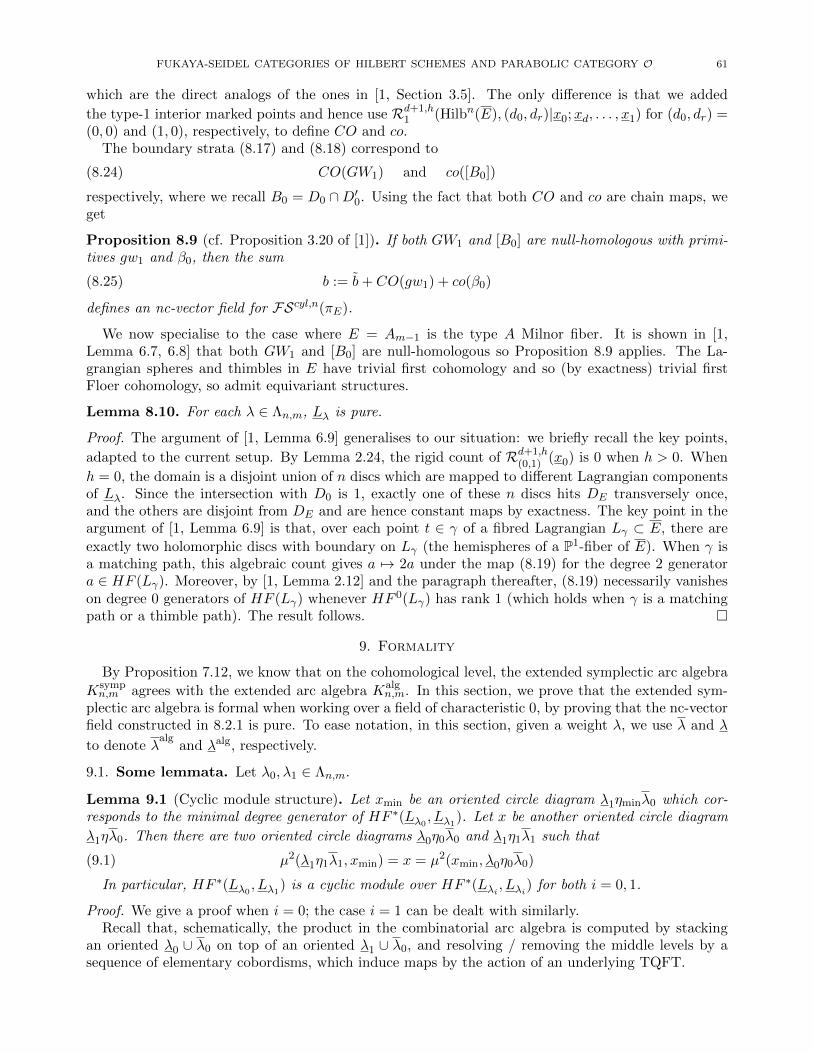
FUKAYA-SEIDEL CATEGORIES OF HILBERT SCHEMES AND PARABOLIC CATEGORY O 61
which are the direct analogs of the ones in [1, Section 3.5]. The only difference is that we added
the type-1 interior marked points and hence use Rd+1,h1 (Hilbn(E), (d0, dr)|x0;xd, . . . , x1) for (d0, dr) =
(0, 0) and (1, 0), respectively, to define CO and co.The boundary strata (8.17) and (8.18) correspond to
CO(GW1) and co([B0])(8.24)
respectively, where we recall B0 = D0 ∩D′0. Using the fact that both CO and co are chain maps, weget
Proposition 8.9 (cf. Proposition 3.20 of [1]). If both GW1 and [B0] are null-homologous with primi-tives gw1 and β0, then the sum
b := b+ CO(gw1) + co(β0)(8.25)
defines an nc-vector field for FScyl,n(πE).
We now specialise to the case where E = Am−1 is the type A Milnor fiber. It is shown in [1,Lemma 6.7, 6.8] that both GW1 and [B0] are null-homologous so Proposition 8.9 applies. The La-grangian spheres and thimbles in E have trivial first cohomology and so (by exactness) trivial firstFloer cohomology, so admit equivariant structures.
Lemma 8.10. For each λ ∈ Λn,m, Lλ is pure.
Proof. The argument of [1, Lemma 6.9] generalises to our situation: we briefly recall the key points,
adapted to the current setup. By Lemma 2.24, the rigid count of Rd+1,h(0,1) (x0) is 0 when h > 0. When
h = 0, the domain is a disjoint union of n discs which are mapped to different Lagrangian componentsof Lλ. Since the intersection with D0 is 1, exactly one of these n discs hits DE transversely once,and the others are disjoint from DE and are hence constant maps by exactness. The key point in theargument of [1, Lemma 6.9] is that, over each point t ∈ γ of a fibred Lagrangian Lγ ⊂ E, there are
exactly two holomorphic discs with boundary on Lγ (the hemispheres of a P1-fiber of E). When γ isa matching path, this algebraic count gives a 7→ 2a under the map (8.19) for the degree 2 generatora ∈ HF (Lγ). Moreover, by [1, Lemma 2.12] and the paragraph thereafter, (8.19) necessarily vanisheson degree 0 generators of HF (Lγ) whenever HF 0(Lγ) has rank 1 (which holds when γ is a matchingpath or a thimble path). The result follows.
9. Formality
By Proposition 7.12, we know that on the cohomological level, the extended symplectic arc algebra
Ksympn,m agrees with the extended arc algebra Kalg
n,m. In this section, we prove that the extended sym-plectic arc algebra is formal when working over a field of characteristic 0, by proving that the nc-vectorfield constructed in 8.2.1 is pure. To ease notation, in this section, given a weight λ, we use λ and λ
to denote λalg
and λalg, respectively.
9.1. Some lemmata. Let λ0, λ1 ∈ Λn,m.
Lemma 9.1 (Cyclic module structure). Let xmin be an oriented circle diagram λ1ηminλ0 which cor-responds to the minimal degree generator of HF ∗(Lλ0
, Lλ1). Let x be another oriented circle diagram
λ1ηλ0. Then there are two oriented circle diagrams λ0η0λ0 and λ1η1λ1 such that
µ2(λ1η1λ1, xmin) = x = µ2(xmin, λ0η0λ0)(9.1)
In particular, HF ∗(Lλ0, Lλ1
) is a cyclic module over HF ∗(Lλi , Lλi) for both i = 0, 1.
Proof. We give a proof when i = 0; the case i = 1 can be dealt with similarly.Recall that, schematically, the product in the combinatorial arc algebra is computed by stacking
an oriented λ0 ∪ λ0 on top of an oriented λ1 ∪ λ0, and resolving / removing the middle levels by asequence of elementary cobordisms, which induce maps by the action of an underlying TQFT.

62 CHEUK YU MAK AND IVAN SMITH
The diagram λ1 ∪ λ0 consists of circles and lines. Let C1, . . . , Ck be the circles, and define forj = 1, . . . , k
Γo,j := γ ∈ λ0|γ is contained in the circle Cj.(9.2)
It is clear that Γo,j 6= ∅ for all j. Let Γo := ∪jΓo,j and Γl := λ0 \ Γo. In particular, if γ ∈ λ0 is a line,then γ ∈ Γl.
The minimal degree generator xmin corresponds to orienting all the circles in λ1∪λ0 counterclockwise(note that the orientations of the arcs in λ1 ∪ λ0 are uniquely determined by the rule (6.12), namely,the remaining ∨ must occupy the rightmost available positions). On the other hand, let Cs1 , . . . , Cstbe the circles in λ1 ∪ λ0 that are oriented clockwise by x. For each j ∈ s1, . . . , st, we pick a singleγj ∈ Γo,j . Now we give λ0 ∪ λ0 the orientation y that is uniquely determined by the property that a
circle C in λ0 ∪ λ0 is oriented clockwise if and only if C contains γj for some j ∈ s1, . . . , st.One feature of the Khovanov TQFT ([24], [25], which is recalled in (6.24) and (6.25)) is that a
counterclockwise circle times a counterclockwise (resp. clockwise) circle is a counterclockwise (resp.clockwise) circle. The analog is true for the Khovanov-type TQFT from [13, 51]. One can check, byapplying the rules underlying the Khovanov-type TQFT from [13, 51], that our prescription ensuresthat we have µ2(xmin, y) = x (see Figure 9.1 for an example).
v
v vvv v v
v v v
v vvv v v
v v v
v vvv
v vv v v v v
v v v vvvvvv vvvv v
Figure 9.1. From left to right: y (top) and xmin (bottom) before taking product; suc-cessively applying two TQFT operations to the first picture; the product x. Clockwiseorientations on circles are indicated by H. We choose γj to be the outermost upperarcs in the 2 circle components of x; this forces the indicated Hs on y.
Lemma 9.2. Let λa be an oriented cap diagram and bλ be an oriented cup diagram. Then we have
µ2(bλλ, λλa) = bλa(9.3)
In particular, the product map
HF (Lλ, Lb)×HF (La, Lλ)→ HF (La, Lb)(9.4)
is nonzero.
Proof. Note that λλa, bλλ and bλa are oriented circle diagrams so the LHS and RHS of (9.3) arewell-defined.
Now we need to justify (9.3). If γ ∈ λ is a half-circle and the component in λλa containing γis a circle C, then by the definition of λ, we know that C is oriented counterclockwise. Similarly,if γ∗ ∈ λ is a half-circle and the component in bλλ containing γ∗ is a circle C ′, then C ′ is orientedcounterclockwise. In this case, when we do the resolution between γ and γ∗ involved in the product,the outcome is also oriented counterclockwise. In other words, the resolution cobordism move doesnot change the orientation (see Figure 9.2)
On the other hand, if the component of λλa containing γ is a line, then we need to first completeit to a circle before computing the product. Moreover, the circle to which it is completed is orientedcounterclockwise (see Figure 9.3). The same holds for bλλ.
Therefore, each type of resolution, and hence the product obtained from a composition of such,does not change the orientations. It implies µ2(bλλ, λλa) = bλa.
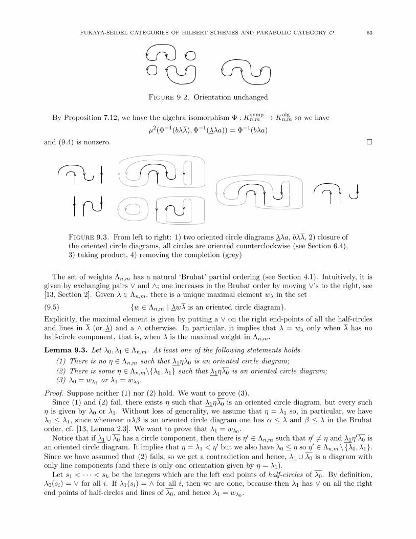
FUKAYA-SEIDEL CATEGORIES OF HILBERT SCHEMES AND PARABOLIC CATEGORY O 63
v vv v v v
v vv
Figure 9.2. Orientation unchanged
By Proposition 7.12, we have the algebra isomorphism Φ : Ksympn,m → Kalg
n,m so we have
µ2(Φ−1(bλλ),Φ−1(λλa)) = Φ−1(bλa)
and (9.4) is nonzero.
v
v v v
v vv
v v v
v vv v
v v
v v vv v v v v
Figure 9.3. From left to right: 1) two oriented circle diagrams λλa, bλλ, 2) closure ofthe oriented circle diagrams, all circles are oriented counterclockwise (see Section 6.4),3) taking product, 4) removing the completion (grey)
The set of weights Λn,m has a natural ‘Bruhat’ partial ordering (see Section 4.1). Intuitively, it isgiven by exchanging pairs ∨ and ∧; one increases in the Bruhat order by moving ∨’s to the right, see[13, Section 2]. Given λ ∈ Λn,m, there is a unique maximal element wλ in the set
w ∈ Λn,m | λwλ is an oriented circle diagram.(9.5)
Explicitly, the maximal element is given by putting a ∨ on the right end-points of all the half-circlesand lines in λ (or λ) and a ∧ otherwise. In particular, it implies that λ = wλ only when λ has nohalf-circle component, that is, when λ is the maximal weight in Λn,m.
Lemma 9.3. Let λ0, λ1 ∈ Λn,m. At least one of the following statements holds.
(1) There is no η ∈ Λn,m such that λ1ηλ0 is an oriented circle diagram;
(2) There is some η ∈ Λn,m\λ0, λ1 such that λ1ηλ0 is an oriented circle diagram;(3) λ0 = wλ1 or λ1 = wλ0.
Proof. Suppose neither (1) nor (2) hold. We want to prove (3).Since (1) and (2) fail, there exists η such that λ1ηλ0 is an oriented circle diagram, but every such
η is given by λ0 or λ1. Without loss of generality, we assume that η = λ1 so, in particular, we haveλ0 ≤ λ1, since whenever αλβ is an oriented circle diagram one has α ≤ λ and β ≤ λ in the Bruhatorder, cf. [13, Lemma 2.3]. We want to prove that λ1 = wλ0 .
Notice that if λ1 ∪λ0 has a circle component, then there is η′ ∈ Λn,m such that η′ 6= η and λ1η′λ0 is
an oriented circle diagram. It implies that η = λ1 < η′ but we also have λ0 ≤ η so η′ ∈ Λn,m \λ0, λ1.Since we have assumed that (2) fails, so we get a contradiction and hence, λ1 ∪ λ0 is a diagram withonly line components (and there is only one orientation given by η = λ1).
Let s1 < · · · < sk be the integers which are the left end points of half-circles of λ0. By definition,λ0(si) = ∨ for all i. If λ1(si) = ∧ for all i, then we are done, because then λ1 has ∨ on all the rightend points of half-circles and lines of λ0, and hence λ1 = wλ0 .

64 CHEUK YU MAK AND IVAN SMITH
If this is not the case, then let sj be the largest among s1, . . . sk such that λ1(sj) = ∨. Let sj + t be
the right end point of the half-circle of λ0 with left end point sj . By definition of λ0, exactly half ofsj + 1, . . . , sj + t − 1 are labelled by ∧ and half by ∨ with respect to λ0. Moreover, all of them lie
in a half-circle of λ0.By the definition of sj , for l = 1, . . . , t− 1, if λ0(sj + l) = ∨, then sj + j ∈ sj+1, . . . , sk so we have
λ1(sj + l) = ∧. Moreover, for λ1ηλ0 to have at least one orientation, we need that λ1(sj + t) = ∧ andfor l = 1, . . . , t − 1, if λ0(sj + l) = ∧, then λ1(sj + l) = ∨ (see Figure 9.4). Now, by the definition of
λ1, we see that λ1ηλ0 has a circle passing through sj and sj + t. This contradicts the fact that λ1ηλ0
does not have circle components.
v v v vvv v v
Figure 9.4. The weight and the cap diagram on top are λ0 and λ0; the weight andthe cup diagram on the bottom are λ1 and λ1.
9.2. Consistent choice of equivariant structures. Let b be the nc vector field constructed inProposition 8.9.
Proposition 9.4. There is a choice of b-equivariant structures on Lλλ∈Λn,m such that b is pure.
Proof. By Lemma 8.10, Lλ is pure for each λ ∈ Λn,m.Any partial order admits a total order refinement. We choose a total ordering (≤T ) on Λn,m that
is compatible with the Bruhat partial ordering ≤. We make choices of b-equivariant structure on theLλ with decreasing order of λ.
Let η ∈ Λn,m and suppose that a b-equivariant structure on Lλ is chosen for all λ >T η, such thatb is pure. We want to choose a b-equivariant structure on Lη such that b is pure on Lλλ≥T η.
We choose a b-equivariant structure on Lη such that the minimal degree element of HF (Lη, Lwη)
has weight equal to the degree. By Lemma 9.1, HF (Lη, Lwη) is cyclic as a module over HF (Lwη , Lwη)
so the weight equals the degree for all pure degree elements in HF (Lη, Lwη).By Lemma 9.2, we have
µ2(ηwηwη, wηwηη) = ηwηη(9.6)
This implies that x := ηwηwη in HF (Lwη , Lη) has weight equal to its degree.
Let xmin be the minimal degree generator of HF (Lwη , Lη). By Lemma 9.1, we know that x =
µ2(xmin, y) for some y ∈ HF (Lwη , Lwη). It means that xmin also has weight equal to its degree, and
hence all elements of HF (Lwη , Lη) have weight equal to their degrees.
Now, suppose that λ >T η but λ 6= wη, and purity holds for all of HF (Lλ′ , Lη), HF (Lη, Lλ′)such that λ′ >T λ. By Lemma 9.3, λ, η satisfies either (1) or (2) of Lemma 9.3. If (1) holds, thenHF (Lλ, Lη) = HF (Lη, Lλ) = 0 so purity is automatic. If (2) holds, let λ′ > λ, η and λ′ 6= λ, η suchthat ηλ′λ is an oriented circle diagram.
By Lemma 9.2, we have
µ2(λλ′λ′, λ′λ′η) = λλ′η(9.7)
This means that λλ′η in HF (Lη, Lλ) has weight equal to its degree. By Lemma 9.1 again, we knowthe minimal degree elements in HF (Lη, Lλ) have weight equal to degree, hence so do all elements in

FUKAYA-SEIDEL CATEGORIES OF HILBERT SCHEMES AND PARABOLIC CATEGORY O 65
HF (Lη, Lλ). The same is true for HF (Lλ, Lη) because Lemma 9.2 also implies that
µ2(ηλ′λ′, λ′λ′λ) = ηλ′λ(9.8)
By induction over the total order, the result follows.
Corollary 9.5. Over a field of characteristic 0, the A∞-endomorphism algebra of the direct sum ofobjects in the collection Lλλ∈Λn,m is formal.
Proof. This follows from Theorem 8.8 and Proposition 9.4.
Proof of Theorem 1.1. Recall the notation for the tuple of Lagrangian thimbles T I from Section 4.
One can argue inductively to show that T (λ)−1(∨) can be generated by Lλ|λ ∈ Λn,m using the exact
triangles constructed in Section 3.2 (compare with Proposition 10.1).We now give the details. When n = 1, Lλ|λ ∈ Λn,m consists of one Lefschetz thimble at the right
most critical point, and all the matching spheres over matching paths whose end points are consecutive
critical values. This collection clearly generates T (λ)−1(∨), by applying Dehn twists in the matchingspheres to the Lefschetz thimble. We now argue inductively. Let k ∈ N+. We assume that for all
n < k, for all m ≥ n and for all λ0 ∈ Λn,m, the Lagrangian tuple T (λ0)−1(∨) can be generated by thecollection Lλ|λ ∈ Λn,m. Now we consider the case n = k, m ≥ n and let λ ∈ Λn,m.
When λ−1(∨) = m− n+ 1, . . . ,m, λ is the maximal weight and we have Lλ = T λ−1(∨).
If λ is not the maximal weight, then there is k ∈ 1, . . . ,m such that λ(k) = ∨ and λ(k + 1) = ∧.Let λ′′ be the weight given by ‘swapping positions k and k + 1’. That is
λ′′(i) =
λ(i) if i 6= k, k + 1∧ if i = k∨ if i = k + 1
(9.9)
Let λ′ ∈ Λn−1,m−2 be the weight given by forgetting the positions k, k + 1.That is
λ′(i) =
λ(i) if i < k
λ(i+ 2) if i ≥ k(9.10)
We define ∪k,k+1λ′ to be the admissible tuple in im(z) ≤ 1 consisting of 1 matching path connecting
k+√−1 and k+ 1 +
√−1 and n− 1 thimble paths from i+
√−1 to i for each i ∈ λ−1(∨) \ k. The
notation suggests that it is obtained from applying a ‘cup functor’ to λ′ in position k, k + 1 in thesense of [2].
By Corollary 3.5, we have the following exact triangle
T (λ′′)−1(∨)[−1]→ L∪k,k+1λ′→ T (λ)−1(∨) → T (λ′′)−1(∨)(9.11)
Note that the second term L∪k,k+1λ′can be generated by Lλ|λ ∈ Λn,m by applying the ‘cup functor’
∪k,k+1 to the induction hypothesis. More precisely, by induction hypothesis, the collection
Lλ|λ ∈ Λn−1,m−2
is sufficient to generate LΓ for all admissible tuple Γ = γ1, . . . , γn such that for all i, γi is a thimblepath from qi +
√−1 to qi for some qi ∈ 1, . . . ,m. Together with Corollary 3.5 (which implies that
the ‘cup functor’ takes exact triangles to exact triangles), we know that the collection
Lλ|λ ∈ Λn,m, λ(k) = ∨, λ(k + 1) = ∧
is sufficient to generate LΓ for all admissible tuple Γ = γ1, . . . , γn such that (see Figure 9.5)
(1) γi ⊂ im(z) ≤ 1 for all i(2) γ1 is a matching path joining k +
√−1 and k + 1 +
√−1
(3) for i > 1, γi is a thimble path from qi +√−1 to qi for some qi ∈ 1, . . . ,m.

66 CHEUK YU MAK AND IVAN SMITH
x x x x x x x x x x x x
x x x x x x
x x x x
x x[1]
[1]
Figure 9.5. The first row represents an exact triangle in the induction hypothesis.The second row is the exact triangle after applying the ‘cup functor’ ∪2,3 to it.
On the other hand, the first and third term of (9.11) has the property that λ′′ > λ. Since Lλ =
T λ−1(∨) when λ is maximal, by (9.11) and a second induction with respect to the Bruhat ordering
starting from the maximal weight, we know that T (λ)−1(∨) can be generated by Lλ|λ ∈ Λn,m.Conversely, Lλ can be generated by T (λ)−1(∨)|λ ∈ Λn,m, either again by directly applying the exact
triangles, or by appeal to Proposition 5.16. Therefore, by Proposition 4.5, we have quasi-equivalences
DπFS(πn,m) ' perf-(End(⊕T (λ)−1(∨))) ' perf-(Ksympn,m ) = perf-(Kalg
n,m)(9.12)
Remark 9.6. Theorem 1.1 and Claim 3.6 together give a new proof of a result of [7], namely that theSerre functor of the constructible derived category of the Grassmannian is given by the action of thecentre of the braid group.
There is an algebra isomorphism Kalgn,m ' (Kalg
n,m)op, given on basis elements by sending an orientedcircle diagram βλα to its reflection αrλβr (see [13, Equation (3.9)]). Together with Theorem 1.1, thisimplies that
Corollary 9.7. For all λ, λ′ ∈ Λn,m, we have
HF (Lλ, Lλ′) = HF (Lλ′ , Lλ)(9.13)
as graded vector spaces.
This is already non-trivial, because Lλ, Lλ′ are not compact Lagrangians, so it is not a priori clearwhy they should satisfy this Poincare duality type of equality (because of the non-trivial wrapping inconstructing the category, the underlying cochain groups are typically not equal).
The algebra isomorphism Kalgn,m ' (Kalg
n,m)op can be understood geometrically: we give a sketch of theargument. By a hyperbolic isometry between the upper half plane and the unit disc, we can assumethe target of πE is the unit disc B. We also assume that the critical values lie on the real line, and thatinfinity in the upper half plane is mapped to
√−1 ∈ ∂B. For example, it can be achieved by applying
the inverse of the hyperbolic isometry f : B1 → H in (5.15). Let ιB : B → B be the reflection along thereal line, which is an anti-symplectic involution of B. We recall that for the construction of (E,ωE) inSection 5.1, ωM is restricted from a product symplectic form ωX . Therefore, by appropriately choosingωR in Lemma 5.4, we can assume that there is an anti-symplectic involution ιE : E → E covering ιB.
Let u : S → YE be a solution that contributes to the A∞ structure of FScyl,n(πE). Let ιS : S → Sbe reflection in the real diameter of the disc, and S the image of S (equipped with the push-forwarddata by ιS). Let ιYE : YE → YE be the anti-symplectic involution induced by ιE . In this case,
ιYE u ιS : S → YE is tautologically a solution to the push-forward equation, which is itself aperturbed pseudo-holomorphic equation. Note, however, that the ordering of the Lagrangian boundaryconditions is reversed on ∂S.
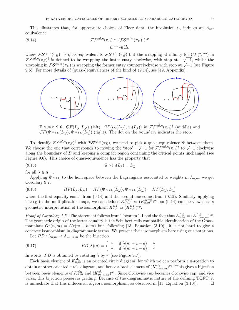
FUKAYA-SEIDEL CATEGORIES OF HILBERT SCHEMES AND PARABOLIC CATEGORY O 67
This illustrates that, for appropriate choices of Floer data, the involution ιE induces an A∞-equivalence
FScyl,n(πE) ' (FScyl,n(πE)†)op(9.14)
L 7→ ιE(L)
where FScyl,n(πE)† is quasi-equivalent to FScyl,n(πE) but the wrapping at infinity for CF (?, ??) inFScyl,n(πE)† is defined to be wrapping the latter entry clockwise, with stop at −
√−1, whilst the
wrapping in FScyl,n(πE) is wrapping the former entry counterclockwise with stop at√−1 (see Figure
9.6). For more details of (quasi-)equivalences of the kind of (9.14), see [49, Appendix].
x x x x x x x x x x x x x x x x x x
Figure 9.6. CF (Lλ, Lλ′) (left), CF (ιE(Lλ′), ιE(Lλ)) in FScyl,n(πE)† (middle) andCF (Ψ ιE(Lλ′),Ψ ιE(Lλ)) (right). The dot on the boundary indicates the stop.
To identify FScyl,n(πE)† with FScyl,n(πE), we need to pick a quasi-equivalence Ψ between them.We choose the one that corresponds to moving the ‘stop’ −
√−1 for FScyl,n(πE)† to
√−1 clockwise
along the boundary of B and keeping a compact region containing the critical points unchanged (seeFigure 9.6). This choice of quasi-equivalence has the property that
Ψ ιE(Lλ) = Lλ(9.15)
for all λ ∈ Λn,m.Applying Ψ ιE to the hom space between the Lagrangians associated to weights in Λn,m, we get
Corollary 9.7:
HF (Lλ, Lλ′) = HF (Ψ ιE(Lλ′),Ψ ιE(Lλ)) = HF (Lλ′ , Lλ)(9.16)
where the first equality comes from (9.14) and the second one comes from (9.15). Similarly, applyingΨ ιE to the multiplication maps, we can deduce Ksymp
n,m ' (Ksympn,m )op, so (9.14) can be viewed as a
geometric interpretation of the isomorphism Kalgn,m ' (Kalg
n,m)op.
Proof of Corollary 1.5. The statement follows from Theorem 1.1 and the fact thatKalgn,m = (Kalg
m−n,m)op.The geometric origin of the latter equality is the Schubert-cells compatible identification of the Grass-mannians Gr(n,m) = Gr(m − n,m) but, following [13, Equation (3.10)], it is not hard to give aconcrete isomorphism in diagrammatic terms. We present their isomorphism here using our notations.
Let PD : Λn,m → Λm−n,m be the bijection
PD(λ)(a) =
∧ if λ(m+ 1− a) = ∨∨ if λ(m+ 1− a) = ∧(9.17)
In words, PD is obtained by rotating λ by π (see Figure 9.7).
Each basis element of Kalgn,m is an oriented circle diagram, for which we can perform a π-rotation to
obtain another oriented circle diagram, and hence a basis element of (Kalgm−n,m)op. This gives a bijection
between basis elements of Kalgn,m and (Kalg
m−n,m)op. Since clockwise cup becomes clockwise cap, and viceversa, this bijection preserves grading. Because of the diagrammatic nature of the defining TQFT, itis immediate that this induces an algebra isomorphism, as observed in [13, Equation (3.10)].

68 CHEUK YU MAK AND IVAN SMITH
∧ ∧ v v ∧ v ∧ v ∧ ∧ v v=
Figure 9.7. Left: a weight λ, Right: the weight PD(λ)
10. Dictionary between Lagrangians and modules
In this section, we summarise the dictionary between certain objects in FScyl,n(Am−1) (or their
Yoneda images as modules over Ksympn,m ) and modules over Kalg
n,m. None of our results rely on thisdictionary: it is simply meant to help orient the interested reader. Given that, we make free use ofClaim 3.6 in this section.
Modules in this section are right modules, which differs from the convention used in [13]. However,
as remarked previously, there is a canonical algebra isomorphism Kalgn,m ' (Kalg
n,m)op, which identifies
the right Kalgn,m-modules used below with the left Kalg
n,m-modules used in [13].For an A∞ or dg category/algebra C, we use perf-C and C-perf to denote the dg category of perfect
right, and respectively left, C modules. We use [C,D] denote the dg category of C-D bimodules. Since
Kalgn,m is homologically smooth, every proper (cohomologically finite) module or bimodule is perfect.
10.1. Indecomposable projectives. For each λ ∈ Λn,m, we define P (λ) to be the submodule of
Kalgn,m generated by the oriented circle diagrams of the form
P (λ) := ⊕Kλalgµα(10.1)
The collection of all P (λ) (together with their grading shifts) is the set of all indecomposable projective
modules of Kalgn,m. Under the isomorphism Ksymp
n,m ' Kalgn,m, P (λ) is the same as the Yoneda embedding
of Lλ as a right Ksympn,m module. Thus, the indecomposable projectives are the Lagrangians associated
to weights.
By [13, Theorem 5.3], the set of all indecomposable injective modules of Kalgn,m is given by
P (λ)∗ := Hom(P (λ),K)(10.2)
where the right module structure is given by fa(m) := f(ma∗) for a ∈ Kalgn,m, m ∈ P (λ) and f ∈ P (λ)∗.
In other words, P (λ)∗ is obtained by pulling back the left module Hom(P (λ),K) via the algebra
isomorphism Kalgn,m = (Kalg
n,m)op. On the symplectic side, up to a grading shift, Hom(P (λ),K) is given bythe Yoneda embedding of τ−1(Lλ) as a left Ksymp
n,m module, where τ is the global monodromy (see Claim
3.6), so P (λ)∗ corresponds to the pull-back of τ−1(Lλ) via the algebra isomorphismKsympn,m = (Ksymp
n,m )op.
In view of the geometric explanation of the equivalence Ksympn,m = (Ksymp
n,m )op given in (9.14), P (λ)∗
is given by the right Yoneda embedding of Ψ ιE τ−1(Lλ).
10.2. Standard modules. For each λ ∈ Λn,m, there is a standard module V (λ) defined in [13,Equation (5.11)]. As a graded vector space, V (λ) is generated by oriented cap diagrams of the form
λα. The collection of all V (λ) gives a full exceptional collection for the dg category of right Kalgn,m
modules and Exti(V (λ0), V (λ1)) 6= 0 for some i only if λ0 < λ1, where < is with respect to the Bruhatpartial ordering.
An inductive construction of a projective resolution of V (λ) is described in [12, Theorem 5.3]. Byidentifying P (λ) with the Yoneda image of Lλ and imitating that inductive construction, we have
Proposition 10.1. The standard module V (λ), as an A∞ module over Kalgn,m = Ksymp
n,m , is quasi-
isomorphic to the Yoneda image of T λ−1(∨) up to grading shift.
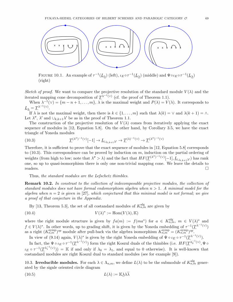
FUKAYA-SEIDEL CATEGORIES OF HILBERT SCHEMES AND PARABOLIC CATEGORY O 69
x x x x x x
x x x x x x x x x x x x
Figure 10.1. An example of τ−1(Lλ) (left), ιE τ−1(Lλ) (middle) and ΨιE τ−1(Lλ)
(right)
Sketch of proof. We want to compare the projective resolution of the standard module V (λ) and the
iterated mapping cone decomposition of T λ−1(∨) (cf. the proof of Theorem 1.1).
When λ−1(∨) = m− n+ 1, . . . ,m, λ is the maximal weight and P (λ) = V (λ). It corresponds to
Lλ = T λ−1(∨).
If λ is not the maximal weight, then there is k ∈ 1, . . . ,m such that λ(k) = ∨ and λ(k + 1) = ∧.Let λ′′, λ′ and ∪k,k+1λ
′ be as in the proof of Theorem 1.1.The construction of the projective resolution of V (λ) comes from iteratively applying the exact
sequence of modules in [12, Equation 5.8]. On the other hand, by Corollary 3.5, we have the exacttriangle of Yoneda modules
T (λ′′)−1(∨)[−1]→ L∪k,k+1λ′→ T (λ)−1(∨) → T (λ′′)−1(∨)(10.3)
Therefore, it is sufficient to prove that the exact sequence of modules in [12, Equation 5.8] correspondsto (10.3). This correspondence can be proved by induction on m, induction on the partial ordering of
weights (from high to low; note that λ′′ > λ) and the fact that HF (T (λ′′)−1(∨)[−1], L∪k,k+1λ′) has rank
one, so up to quasi-isomorphism there is only one non-trivial mapping cone. We leave the details toreaders.
Thus, the standard modules are the Lefschetz thimbles.
Remark 10.2. In constrast to the collection of indecomposable projective modules, the collection ofstandard modules does not have formal endomorphism algebra when n > 1. A minimal model for thealgebra when n = 2 is given in [27], which conjectured that this minimal model is not formal; we givea proof of that conjecture in the Appendix.
By [13, Theorem 5.3], the set of all costandard modules of Kalgn,m are given by
V (λ)∗ := Hom(V (λ),K)(10.4)
where the right module structure is given by fa(m) := f(ma∗) for a ∈ Kalgn,m, m ∈ V (λ)∗ and
f ∈ V (λ)∗. In other words, up to grading shift, it is given by the Yoneda embedding of τ−1(T λ−1(∨))
as a right (Ksympn,m )op module after pull-back via the algebra isomorphism Ksymp
n,m = (Ksympn,m )op.
In view of (9.14) again, V (λ)∗ is given by the right Yoneda embedding of Ψ ιE τ−1(T λ−1(∨)).
In fact, the Ψ ιE τ−1(T λ−1(∨)) form the right Koszul duals of the thimbles (i.e. HF (T λ
−10 (∨),Ψ
ιE τ−1(T λ−11 (∨))) = K if and only if λ0 = λ1, and equal to 0 otherwise). It is well-known that
costandard modules are right Koszul dual to standard modules (see for example [9]).
10.3. Irreducible modules. For each λ ∈ Λn,m, we define L(λ) to be the submodule of Kalgn,m gener-
ated by the signle oriented circle diagram
L(λ) := Kλλλ(10.5)

70 CHEUK YU MAK AND IVAN SMITH
x x x x x x
x x x x x x x x x x x x
Figure 10.2. An example of τ−1(T λ−1(∨)) (left), ιE τ−1(T λ
−1(∨)) (middle) and Ψ ιE τ−1(T λ
−1(∨)) (right)
The collection of all L(λ) is the set of all irreducible modules of Kalgn,m.
It is not immediately clear in our context which Lagrangians correspond to the irreducible modules.In view of the work of [18], and the ‘topological model’ for the compact core of the space Yn,m arisingfrom its description as a quiver variety (see e.g. [2]), it is reasonable to believe that one can enlargethe category FScyl,n(E) to allow Lagrangian discs that intersect exactly one of the Lλλ once andare disjoint from the others. These would be the analogues of ‘cocore discs’ over the components ofthe skeleton of a plumbing of cotangent bundles, and the Yoneda images of these Lagrangian discs arenatural candidates for the irreducible modules.
11. Symplectic annular Khovanov homology
This section gives an application of our main results to link homology theories in the sense ofKhovanov. Suppose m = 2n. A braid β ∈ Brn in the n-string braid group defines bimodules
P(j)β over each of the extended arc algebras Kalg
j,n with 0 ≤ j ≤ n. One can combine a theorem of
Roberts [39] with deep recent work of Beliakova, Putyra and Wehrli [8] to infer that there is a spectral
sequence ⊕jHH∗(P (j)β ) ⇒ Kh(κ(β)), where κ(β) is the link closure of β, and where Kh(κ) is the
Khovanov homology [24] of the link κ ⊂ S3, constructed as a categorification of the Jones polynomial.It is by now classical that Khovanov homology can be understood as a certain morphism group
Extperf-Halg
n,2n(P, (β × id)(P )) in the derived category of modules over the compact arc algebra Halg
n,2n,
see [25], where β × id ∈ Br2n belongs to the 2n-string braid group and P is a particular projective.From the viewpoint of the (extended) arc algebras, the existence of such a spectral sequence is rathermysterious. The purpose of this section is to give a transparent account of why it should exist, starting
from a new semi-orthogonal decomposition of perf -Kalgn,2n which we shall derive from the geometric
viewpoint afforded by Theorem 1.1.We assume m = 2n in Sections 11 and 12 unless stated otherwise.
11.1. The annular symplectic theory. Let hs ∈ Λn,m be the weight such that hs−1(∨) = 1, . . . , n.The corresponding tuple Lhs is called the ‘horseshoe’ Lagrangian tuple and the Lagrangian Sym(Lhs) ⊂Yn,m is the horseshoe Lagrangian from [47, 1]. Let Brn be the braid group on n strands. The paper
[47] associates to each element β ∈ Brn a symplectomorphism φ(n)β : Yn,m → Yn,m, and defines the
symplectic Khovanov cohomology of the braid closure κ = κ(β) of β to be
Khsymp(κ(β)) := HF (Sym(Lhs), φ(n)β (Sym(Lhs)))(11.1)
The main result of [47] is that Khsymp(κ(β)) is a link invariant, i.e. it is independent of the represen-tation of κ as a braid closure.
One can give an equivalent definition of symplectic Khovanov cohomology using Lhs instead ofits product Sym(Lhs). Let E := Am−1 denote the Milnor fiber. To each simple braid element σi

FUKAYA-SEIDEL CATEGORIES OF HILBERT SCHEMES AND PARABOLIC CATEGORY O 71
we associate the symplectomorphism φσi : E → E given by the Dehn twist along the ith matchingsphere (lying above the line joining i+
√−1 and i+ 1 +
√−1). This defines a representation Brm →
π0Sympct(E). Let Brn → Brm be the embedding of the left n strands. We have the restrictedrepresentation Brn → π0Sympct(E) so each braid β ∈ Brn determines a symplectomorphism φβ of Ethat acts as the identity on the ‘right half’.
Then [31]
Khsymp(κ(β)) = HF (Lhs, φβ(Lhs)).(11.2)
Let E1/2 be the An−1-Milnor fiber with its standard Lefschetz fibration πE1/2. We can define the
symplectomorphism φβ of E1/2 for β ∈ Brn accordingly. Then φβ induces an A∞ endofunctor of
FScyl,j(πE1/2), and hence an A∞-bimodule P
(j)β over FScyl,j(πE1/2
).
Definition 11.1. The symplectic annular Khovanov homology of the braid β ∈ Brn is the direct sumof Hochschild homology groups
AKhsymp(β) := ⊕nj=0HH∗(FScyl,j(πE1/2), P
(j)β )(11.3)
where, by convention, FScyl,j(πE1/2) = K and P
(j)β = K is the diagonal bimodule when j = 0 (cf.
Remark 1.2).
Symplectic annular Khovanov homology is clearly a braid invariant. It is not an invariant of thelink closure of the braid. Its definition is motivated by the fact that combinatorial annular Khovanovhomology, originally defined by a diagrammatic calculus for links in a solid torus [4], is itself isomorphicto a direct sum of Hochschild homologies of braid bimodules over the extended arc algebras, a recenttheorem of [8] establishing a conjecture due to [6]. Indeed, Theorem 1.1 and the same formalityarguments for bimodules as in [2] would prove that
Proposition 11.2. AKhsymp(β) is isomorphic to annular Khovanov homology when K has charac-teristic 0.
We will prove Theorem 1.9 by constructing a spectral sequence AKhsymp(β)⇒ Khsymp(κ(β)).
Remark 11.3. One could also define a braid invariant as the direct sum of fixed point Floer homologiesof φβ on Yj,n over j ∈ 0, . . . , n (where ‘partial wrapping’ would remove fixed points at infinity). Itseems likely that this geometric definition would recover that of Definition 11.1, but establishing suchan isomorphism is beyond the scope of this paper. See [43] for closely related results.
Remark 11.4. There is an sl2 action on AKhsymp(β), by combining [21] and Proposition 11.2, whichimplies a rank inequality
rank(HH∗(FScyl,j(πE1/2), P
(j)β )) ≤ rank(HH∗(FScyl,j+1(πE1/2
), P(j+1)β ))
for all j < n/2. Coupled with Remark 11.3, this predicts a non-trivial existence result for periodicpoints of the symplectomorphisms of Yj,n associated to braids. It would be interesting to construct thesl2 action symplectic-geometrically.
11.2. Embedding of algebras. Let E := Am−1 and πE be the standard Lefschetz fibration. Let
W1 := re(z) < n + 12 and W2 := re(z) > n + 1
2. Note that FScyl,jW1(πE) = FScyl,j(πE1/2
). As
explained in Section 3.2, there is a faithful A∞ functor tK : FScyl,jW1(πE) → FScyl,n(πE) for each
object K of FScyl,n−jW2(πE).
By essentially the same argument, we can prove that
HF (L0 tK0, L1 tK1) = HF (L0, L1)⊗HF (K0,K1)(11.4)
for Li ∈ FScyl,jW1
(πE) and Ki ∈ FScyl,jW2
(πE). Varying either the Li or Ki, Floer multiplication amongstthe corresponding groups also respects the tensor product structure. Let 0 ≤ j ≤ n be an integer.
For each λ ∈ Λj,n, one can define an object Lλ in FScyl,jW1(πE) by forgetting the right n critical values
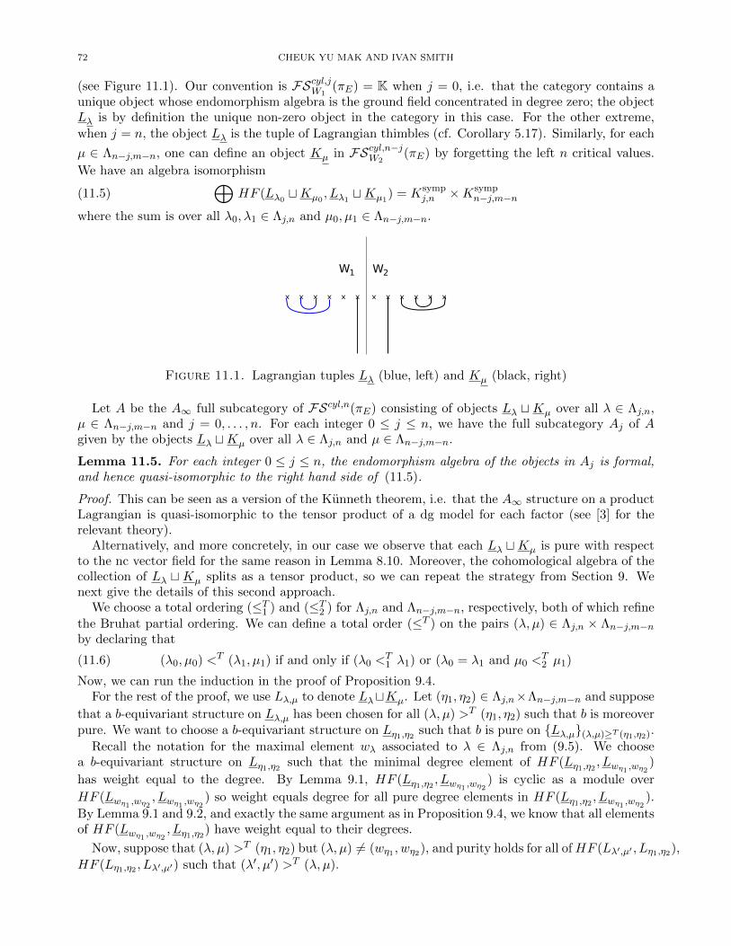
72 CHEUK YU MAK AND IVAN SMITH
(see Figure 11.1). Our convention is FScyl,jW1(πE) = K when j = 0, i.e. that the category contains a
unique object whose endomorphism algebra is the ground field concentrated in degree zero; the objectLλ is by definition the unique non-zero object in the category in this case. For the other extreme,
when j = n, the object Lλ is the tuple of Lagrangian thimbles (cf. Corollary 5.17). Similarly, for each
µ ∈ Λn−j,m−n, one can define an object Kµ in FScyl,n−jW2(πE) by forgetting the left n critical values.
We have an algebra isomorphism⊕HF (Lλ0
tKµ0, Lλ1
tKµ1) = Ksymp
j,n ×Ksympn−j,m−n(11.5)
where the sum is over all λ0, λ1 ∈ Λj,n and µ0, µ1 ∈ Λn−j,m−n.
x x x x x x x x x x x x
W2W1
Figure 11.1. Lagrangian tuples Lλ (blue, left) and Kµ (black, right)
Let A be the A∞ full subcategory of FScyl,n(πE) consisting of objects Lλ tKµ over all λ ∈ Λj,n,µ ∈ Λn−j,m−n and j = 0, . . . , n. For each integer 0 ≤ j ≤ n, we have the full subcategory Aj of Agiven by the objects Lλ tKµ over all λ ∈ Λj,n and µ ∈ Λn−j,m−n.
Lemma 11.5. For each integer 0 ≤ j ≤ n, the endomorphism algebra of the objects in Aj is formal,and hence quasi-isomorphic to the right hand side of (11.5).
Proof. This can be seen as a version of the Kunneth theorem, i.e. that the A∞ structure on a productLagrangian is quasi-isomorphic to the tensor product of a dg model for each factor (see [3] for therelevant theory).
Alternatively, and more concretely, in our case we observe that each Lλ tKµ is pure with respectto the nc vector field for the same reason in Lemma 8.10. Moreover, the cohomological algebra of thecollection of Lλ t Kµ splits as a tensor product, so we can repeat the strategy from Section 9. Wenext give the details of this second approach.
We choose a total ordering (≤T1 ) and (≤T2 ) for Λj,n and Λn−j,m−n, respectively, both of which refinethe Bruhat partial ordering. We can define a total order (≤T ) on the pairs (λ, µ) ∈ Λj,n × Λn−j,m−nby declaring that
(λ0, µ0) <T (λ1, µ1) if and only if (λ0 <T1 λ1) or (λ0 = λ1 and µ0 <
T2 µ1)(11.6)
Now, we can run the induction in the proof of Proposition 9.4.For the rest of the proof, we use Lλ,µ to denote LλtKµ. Let (η1, η2) ∈ Λj,n×Λn−j,m−n and suppose
that a b-equivariant structure on Lλ,µ has been chosen for all (λ, µ) >T (η1, η2) such that b is moreoverpure. We want to choose a b-equivariant structure on Lη1,η2
such that b is pure on Lλ,µ(λ,µ)≥T (η1,η2).
Recall the notation for the maximal element wλ associated to λ ∈ Λj,n from (9.5). We choosea b-equivariant structure on Lη1,η2
such that the minimal degree element of HF (Lη1,η2, Lwη1 ,wη2
)
has weight equal to the degree. By Lemma 9.1, HF (Lη1,η2, Lwη1 ,wη2
) is cyclic as a module over
HF (Lwη1 ,wη2, Lwη1 ,wη2
) so weight equals degree for all pure degree elements in HF (Lη1,η2, Lwη1 ,wη2
).
By Lemma 9.1 and 9.2, and exactly the same argument as in Proposition 9.4, we know that all elementsof HF (Lwη1 ,wη2
, Lη1,η2) have weight equal to their degrees.
Now, suppose that (λ, µ) >T (η1, η2) but (λ, µ) 6= (wη1 , wη2), and purity holds for all ofHF (Lλ′,µ′ , Lη1,η2),
HF (Lη1,η2 , Lλ′,µ′) such that (λ′, µ′) >T (λ, µ).

FUKAYA-SEIDEL CATEGORIES OF HILBERT SCHEMES AND PARABOLIC CATEGORY O 73
Claim 11.6. If HF (Lλ,µ, Lη1,η2) 6= 0, then there exists (λ′, µ′) >T (λ, µ) such that both λλ′η1 andµµ′η2 are oriented circle diagrams.
Assuming Claim 11.6, one can show that purity holds also for HF (Lλ,µ, Lη1,η2), HF (Lη1,η2 , Lλ,µ)exactly as in the last two paragraphs of the proof of Proposition 9.4. Therefore, the result follows byinduction.
Proof of Claim 11.6. By assumption, we have
(wη1 , wη2) >T (λ, µ) >T (η1, η2)(11.7)
By the definition of >T , we have λ = η1 or λ >T1 η1.If λ = η1, then µ >T2 η2. If µ 6= wη2 , then by (2) of Lemma 9.3, there exists µ′ >T2 µ, η2 such that
µµ′η2 is an oriented circle diagram. We can take λ′ = η1 so that we have (λ′, µ′) >T (λ, µ) and both
λλ′η1 and µµ′η2 are oriented circle diagrams.If λ = η1 and µ = wη2 , then by (11.7), we have η1 6= wη1 (in fact, ν = wν only when ν is the
maximal weight, see (9.5)). In this case, we can take (λ′, µ′) = (wη1 , wη2).If λ >T1 η1, then either λ = wη1 or λ 6= wη1 . If λ 6= wη1 , then by (2) of Lemma 9.3, there exists
λ′ >T1 λ, η1 such that λλ′η1 is an oriented circle diagram. By HF (Lλ,µ, Lη1,η2) 6= 0, there exists µ′
such that µµ′η2 is an oriented circle diagram. We can pick any such µ′ because (λ′, µ′) >T (λ, µ) no
matter which µ′ we pick.If λ >T1 η1 but λ = wη1 , then we pick λ′ = λ = wη1 . Since (wη1 , wη2) >T (λ, µ), we have µ <T2 wη2 .
If η2 6= wµ, then by (2) of Lemma 9.3, there exists µ′ >T2 µ, η2 such that µµ′η2 is an oriented circle
diagram so we have done. If η2 = wµ, then µ <T2 η2 so we can take µ′ = η2 becasue it implies that(λ′, µ′) = (wη1 , η2) >T (wη1 , µ) = (λ, µ) and both λλ′η1 and µµ′η2 are oriented circle diagrams.
This completes the proof.
It is not clear whether the endomorphism algebra of the direct sum of all the objects in A is formalor not. However, the dg category of perfect modules perf-A is formal in the following weaker sense.
Lemma 11.7. perf-A is quasi-equivalent to perf-Kalgn,m.
Proof. By iteratively applying exact triangles, we see that the objects in Aj can generate thimbles
T = T1, . . . , Tn in FScyl,n(πE) such that j of the Ti’s are contained in π−1E (W1), and the remaining
n− j are contained in π−1E (W2). Therefore, every thimble of FScyl,n(πE) can be generated by objects
in A, so the result follows.
Lemma 11.8. Let X0 ∈ Aj0 and X1 ∈ Aj1. If HF (X0, X1) 6= 0, then j0 ≥ j1. As a result,〈An, . . . , A0〉 is a semi-orthogonal decomposition of A.
Proof. It is clear that CF (X0, X1) = 0 if j0 < j1, because of the definition of Floer cochains viapositive isotopies along R = ∂H.
Theorem 11.9. perf-Kalgn,m admits a semi-orthogonal decomposition 〈perf-An, . . . , perf-A0〉, where for
each j, perf-Aj is quasi-equivalent to perf-(Kalgj,n ×K
algn−j,m−n).
Proof. This immediately follows from Lemmas 11.5, 11.7 and 11.8.
Theorem 11.9 categorifies the identity(mn
)=∑n
j=0
(nj
)(m−nn−j
)for ranks of Grothendieck groups.
Remark 11.10. Even though we are primarily interested in the case m = 2n in this section, Theorem11.9 holds for all n < m. This algebraic result seems to be new and may be of independent interest.
We need another full subcategory of FScyl,n(πE) that is analogous to A. Let
W !2 := n+
1
2< re(z) < m+
1
2and im(z) < 2 ∪ re(z) < m+
1
2and im(z) <
1
2(11.8)
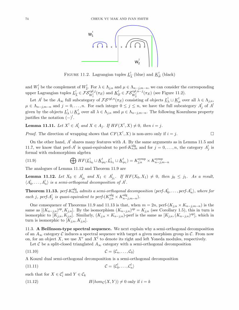
74 CHEUK YU MAK AND IVAN SMITH
x x x x x x x x x x x x
W2!
W1!
Figure 11.2. Lagrangian tuples L!λ
(blue) and K !µ (black)
and W !1 be the complement of W !
2. For λ ∈ Λj,n and µ ∈ Λn−j,m−n, we can consider the corresponding
upper Lagrangian tuples L!λ∈ FScyl,j
W !1
(πE) and K !µ ∈ FS
cyl,n−jW !
2(πE) (see Figure 11.2).
Let A! be the A∞ full subcategory of FScyl,n(πE) consisting of objects L!λ tK !
µ over all λ ∈ Λj,n,
µ ∈ Λn−j,m−n and j = 0, . . . , n. For each integer 0 ≤ j ≤ n, we have the full subcategory A!j of A!
given by the objects L!λ tK !
µ over all λ ∈ Λj,n and µ ∈ Λn−j,m−n. The following Koszulness property
justifies the notation (−)!.
Lemma 11.11. Let X ! ∈ A!i and X ∈ Aj. If HF (X !, X) 6= 0, then i = j.
Proof. The direction of wrapping shows that CF (X !, X) is non-zero only if i = j.
On the other hand, A! shares many features with A. By the same arguments as in Lemma 11.5 and
11.7, we know that perf-A! is quasi-equivalent to perf-Kalgn,m and for j = 0, . . . , n, the category A!
j isformal with endomorphism algebra⊕
HF (L!λ0tK !
µ0, L!
λ1tK !
µ1) = Ksymp
j,n ×Ksympn−j,m−n(11.9)
The analogues of Lemma 11.12 and Theorem 11.9 are
Lemma 11.12. Let X0 ∈ A!j0
and X1 ∈ A!j1
. If HF (X0, X1) 6= 0, then j0 ≤ j1. As a result,
〈A!0, . . . , A
!n〉 is a semi-orthogonal decomposition of A!.
Theorem 11.13. perf-Kalgn,m admits a semi-orthogonal decomposition 〈perf-A!
0, . . . , perf-A!n〉, where for
each j, perf-A!j is quasi-equivalent to perf-(Kalg
j,n ×Kalgn−j,m−n).
One consequence of Theorems 11.9 and 11.13 is that, when m = 2n, perf-(Kj,n ×Kn−j,m−n) is thesame as [(Kn−j,n)op,Kj,n]. By the isomorphism (Kn−j,n)op = Kj,n (see Corollary 1.5), this in turn isisomorphic to [Kj,n,Kj,n]. Similarly, (Kj,n ×Kn−j,n)-perf is the same as [Kj,n, (Kn−j,n)op], which inturn is isomorphic to [Kj,n,Kj,n].
11.3. A Beilinson-type spectral sequence. We next explain why a semi-orthogonal decompositionof an A∞ category C induces a spectral sequence with target a given morphism group in C. From nowon, for an object X, we use Xr and X l to denote its right and left Yoneda modules, respectively.
Let C be a split-closed trianglated A∞ category with a semi-orthogonal decomposition
C = 〈Cn, . . . , C0〉(11.10)
A Koszul dual semi-orthogonal decomposition is a semi-orthogonal decomposition
C = 〈C!0, . . . , C!
n〉(11.11)
such that for X ∈ C!i and Y ∈ Ck
H(homC(X,Y )) 6= 0 only if i = k(11.12)
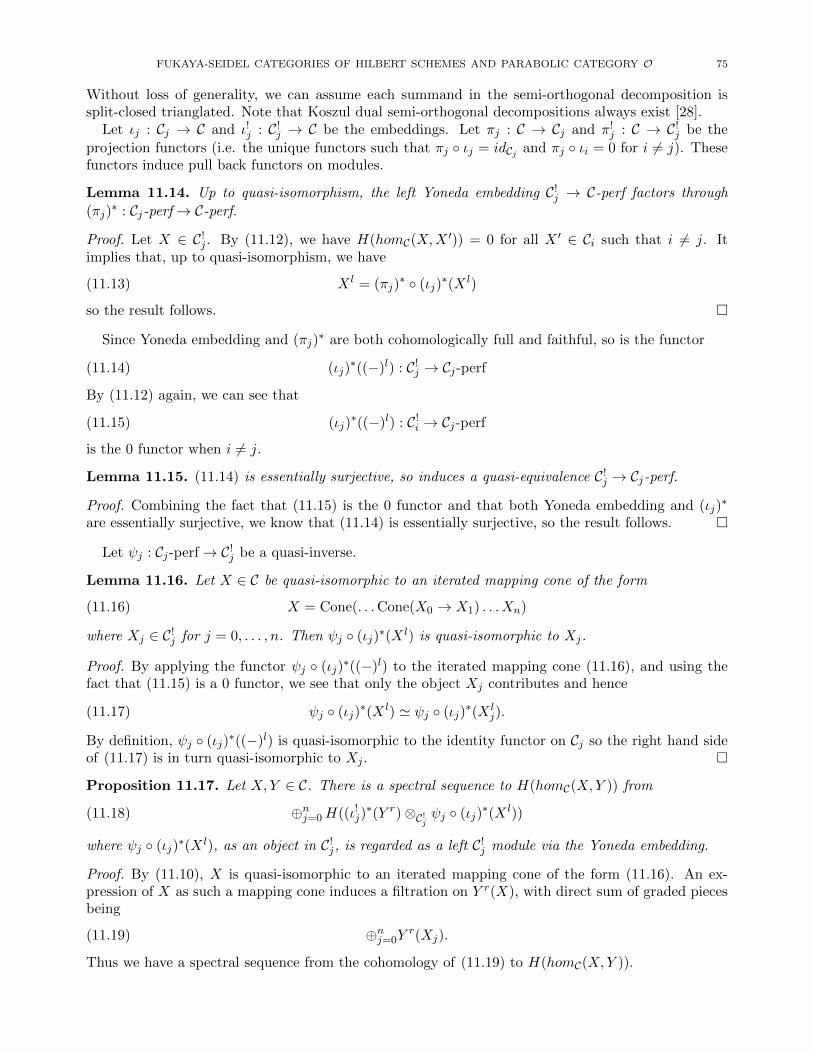
FUKAYA-SEIDEL CATEGORIES OF HILBERT SCHEMES AND PARABOLIC CATEGORY O 75
Without loss of generality, we can assume each summand in the semi-orthogonal decomposition issplit-closed trianglated. Note that Koszul dual semi-orthogonal decompositions always exist [28].
Let ιj : Cj → C and ι!j : C!j → C be the embeddings. Let πj : C → Cj and π!
j : C → C!j be the
projection functors (i.e. the unique functors such that πj ιj = idCj and πj ιi = 0 for i 6= j). Thesefunctors induce pull back functors on modules.
Lemma 11.14. Up to quasi-isomorphism, the left Yoneda embedding C!j → C-perf factors through
(πj)∗ : Cj-perf→ C-perf.
Proof. Let X ∈ C!j . By (11.12), we have H(homC(X,X
′)) = 0 for all X ′ ∈ Ci such that i 6= j. Itimplies that, up to quasi-isomorphism, we have
X l = (πj)∗ (ιj)
∗(X l)(11.13)
so the result follows.
Since Yoneda embedding and (πj)∗ are both cohomologically full and faithful, so is the functor
(ιj)∗((−)l) : C!
j → Cj-perf(11.14)
By (11.12) again, we can see that
(ιj)∗((−)l) : C!
i → Cj-perf(11.15)
is the 0 functor when i 6= j.
Lemma 11.15. (11.14) is essentially surjective, so induces a quasi-equivalence C!j → Cj-perf.
Proof. Combining the fact that (11.15) is the 0 functor and that both Yoneda embedding and (ιj)∗
are essentially surjective, we know that (11.14) is essentially surjective, so the result follows.
Let ψj : Cj-perf→ C!j be a quasi-inverse.
Lemma 11.16. Let X ∈ C be quasi-isomorphic to an iterated mapping cone of the form
X = Cone(. . .Cone(X0 → X1) . . . Xn)(11.16)
where Xj ∈ C!j for j = 0, . . . , n. Then ψj (ιj)
∗(X l) is quasi-isomorphic to Xj.
Proof. By applying the functor ψj (ιj)∗((−)l) to the iterated mapping cone (11.16), and using the
fact that (11.15) is a 0 functor, we see that only the object Xj contributes and hence
ψj (ιj)∗(X l) ' ψj (ιj)
∗(X lj).(11.17)
By definition, ψj (ιj)∗((−)l) is quasi-isomorphic to the identity functor on Cj so the right hand side
of (11.17) is in turn quasi-isomorphic to Xj .
Proposition 11.17. Let X,Y ∈ C. There is a spectral sequence to H(homC(X,Y )) from
⊕nj=0H((ι!j)∗(Y r)⊗C!
jψj (ιj)
∗(X l))(11.18)
where ψj (ιj)∗(X l), as an object in C!
j, is regarded as a left C!j module via the Yoneda embedding.
Proof. By (11.10), X is quasi-isomorphic to an iterated mapping cone of the form (11.16). An ex-pression of X as such a mapping cone induces a filtration on Y r(X), with direct sum of graded piecesbeing
⊕nj=0Yr(Xj).(11.19)
Thus we have a spectral sequence from the cohomology of (11.19) to H(homC(X,Y )).

76 CHEUK YU MAK AND IVAN SMITH
On the other hand, we have quasi-isomorphisms of cochain complexes
Y r(Xj) = (ι!j)∗(Y r)(Xj)(11.20)
= (ι!j)∗(Y r)(ψj (ιj)
∗(X l))(11.21)
= (ι!j)∗(Y r)⊗C!
jψj (ιj)
∗(X l)(11.22)
where the second quasi-isomorphism comes from Lemma 11.16, and the other quasi-isomorphismscome from the definitions of the objects involved.
Remark 11.18. In the extreme case where each Cj (and C!j) is an exceptional object, the semi-
orthogonal decomposition is a full exceptional collection and Proposition 11.17 reduces to the well-known Beilison type spectral sequence (cf. [40, Section (5l)]).
12. From annular to ordinary Khovanov homology
In this section, we explain how to apply Proposition 11.17 to the semi-orthogonal decompositionsin Theorem 11.9, 11.13 to obtain a spectral sequence from annular to ordinary (symplectic) Khovanovhomology.
Recall that for an A∞ or dg category/algebra C, the Hochschild homology of a C-C bimodule P isdefined to be
HH∗(C, P ) := H(∆C ⊗C-C P )(12.1)
where ∆C is the diagonal bimodule and ⊗C-C is the derived tensor product over [C, C]. Equivalently,∆C defines a right C ⊗ Cop module and P defines a left C ⊗ Cop module, and we have
HH∗(C, P ) := H(∆C ⊗C⊗Cop P )(12.2)
The fact that Hochschild homology groups appear in the first page of a spectral sequence to sym-plectic Khovanov cohomology arises from a relation between the horseshoe Lagrangian and the di-agonal bimodule, that we explain next. More precisely, in section 12.1, we compute (ιj)
∗(Llhs) and
(ι!j)∗(φβ(Lhs)
r) for the embeddings ιj : Aj → FScyl,n(πE) and ι!j : A!j → FScyl,n(πE). Then, we
describe the quasi-inverse ψj and complete the proof of Theorem 1.9 in Section 12.2.
12.1. Horseshoe Lagrangian tuple and diagonal bimodule. Recall that we have the pull-backfunctor
(ιj)∗ : FScyl,n(πE)-perf→ Aj-perf ' [Kj,n,Kj,n](12.3)
The following is the key technical result.
Proposition 12.1. Up to grading shift, (ιj)∗(Llhs) is quasi-isomorphic to the diagonal Kj,n-bimodule.
We are going to divide the proof into two steps. First, we will show that (ιj)∗(Llhs) coincides with
the diagonal bimodule (up to grading shift) on the cohomological level. Then, we will explain how toadapt the strategy in Section 9 to prove that this bimodule is formal. For all the Lagrangian tuples inthe proof, we continue to use our grading convention (6.8) and the cost is that we will see eventuallythat (ιj)
∗(Llhs) corresponds to the diagonal bimodule shifted by n−j instead of the diagonal bimodule.
This arises from the fact that there are n− j matching paths of (ιj)∗(Llhs) being oriented clockwise in
the sense of the algebraic extended arc algebra (see Remark 12.5).Let µ ∈ Λn−j,n and define 1 ≤ cµ,1 < · · · < cµ,n−j ≤ n as in the beginning of Section 6.1. Let
cµ,i1 < · · · < cµ,is be all the good points. Let
T := n+ 1− cµ,il |l = 1, . . . , s(12.4)
S := 1, . . . , n ∪ (T +1
3) ∪ (T +
2
3)(12.5)

FUKAYA-SEIDEL CATEGORIES OF HILBERT SCHEMES AND PARABOLIC CATEGORY O 77
We define (µ+)′, (µ−)′ : S → ∨,∧ by
(µ+)′(a) =
PD(µ)(a) if a ∈ 1, . . . , n \ T∨ if a ∈ T∧ if a ∈ (T + 1
3) ∪ (T + 23)
(12.6)
and
(µ−)′(a) =
∨ if a ∈ T + 1
3∧ otherwise
(12.7)
There is a unique order preserving bijective map (the order induced as a subset of R) f : 1, . . . , n+2s → S. Let µ+ := (µ+)′ f ∈ Λj+s,n+2s and µ− := (µ−)′ f ∈ Λs,n+2s. For λ ∈ Λj,n, we define(λ t µ−)′ : S → ∨,∧ by
(λ t µ−)′(a) =
λ(a) if a ∈ 1, . . . , n
(µ−)′(a) if a ∈ (T + 13) ∪ (T + 2
3)(12.8)
and let λ t µ− := (λ t µ−)′ f ∈ Λj+s,n+2s. Note that both µ+ and λ t µ− lie in Λj+s,n+2s.
Lemma 12.2. For λ ∈ Λj,n and µ ∈ Λn−j,n, we have vector space isomorphisms
HF k+n−j−s(Lhs, ιj(Lλ,Kµ)) = HF k(Lµ+ , Lλtµ−)(12.9)
for all k. (Here n− j − s is the number of thimble paths in Kµ.)
The importance of Lemma 12.2 is that the right hand side of (12.9) is part of the symplecticextended arc algebra. We will see later how to use (12.9), and the identification of the symplectic andalgebraic extended arc algebras (Proposition 7.12), to compute the bimodule multiplication map of(ιj)∗(Llhs).
Proof of Lemma 12.2. We use an upper matching to represent Lhs and a lower matching to representKµ (see the first picture of Figure 12.1). Now, we apply a symplectomorphism to ‘move the right halfto the top’ and make all the matching paths of Lhs be straight line segments (see the second pictureof Figure 12.1). For each matching path of Kµ, we apply a further symplectomorphism to ‘bend it to
the right’ and make the two end points become n+ 1− cµ,il + 13 +√−1 and n+ 1− cµ,il + 2
3 +√−1
(see the third picture of Figure 12.1). Then, we remove all critical values contained in the thimblepaths of Kµ and all the paths that contain these critical values (see the fourth picture of Figure 12.1).Finally, for those matching paths of Lhs that do not intersect with a matching path of Kµ, we bendthem to the right and turn them into thimble paths (see the fifth picture of Figure 12.1).
x x x x x x ∧ v v v ∧ ∧ x x x x x x x x x x x x
x x x x x x x x x x x x
Figure 12.1. Turning Lhs (red) and Kµ (black) to Lµ+ (red) and Lµ− (black), respectively

78 CHEUK YU MAK AND IVAN SMITH
After this procedure, the set of critical values (the crosses and black dots in Figure 12.1) is exactlyS, and we identify it with 1, . . . , n+ 2s by f . The Lagrangian tuples Lhs and Kµ become Lµ+ andLµ− respectively.
If we now add in a lower matching of Lλ that does not intersect with Lµ− , then together withLµ− we obtain a representative of Lλtµ− (see the second picture of Figure 12.2). Moreover, fordegree reasons (either all generators have odd degree, or all have even degree), both the cochainmodel CF (Lhs, ιj(Lλ,Kµ)) and CF (Lµ+ , Lλtµ−) have vanishing differentials. Furthermore, there isa identification of the generators by sending a generator x of CF (Lµ+ , Lλtµ−) to the generator y ofCF (Lhs, ιj(Lλ,Kµ)) such that πE(y) is the union of πE(x) and the end points of the thimble paths ofKµ (Figure 12.2). This identification increases the grading by the number of points added, which isn− j − s. It completes the proof.
x x x x x x ∧ ∧ v v ∧ v ∧ v ∧ ∧ v vx x x x x x ∧ ∧ v v ∧ v
Figure 12.2. CF (Lhs, ιj(Lλ,Kµ)) (left) and CF (Lµ+ , Lλtµ−) (right)
To prove Lemma 12.2, it suffices to consider a lower matching of Lλ to give a representative ofLλtµ− . However, for this representative, there may be nested circles in the union of matching andthimble paths of Lµ+ and Lλtµ− , which will be inconvenient later on. By possibly sliding the lowermatching of Lλ cross some matchings of Lµ− (and Lλ itself), we can choose a representative L
λtµ−of Lλtµ− with no nested circles (see the second picture of Figure 12.3). This corresponds to choosinganother representative L
λtµ of ιj(Lλ,Kµ), by sliding across some matching paths of Kµ (see the
first picture of Figure 12.3). For these representatives, we still have the (grading shifting) cochainisomorphism with 0 differential
CF ∗+n−j−s(Lhs, Lλtµ) = CF ∗(Lµ+ , Lλtµ−
)(12.10)
which is again given by sending a generator x of CF (Lµ+ , Lλtµ−
) to the generator y of CF (Lhs, Lλtµ)
such that πE(y) is the union of πE(x) and the end points of the thimble paths of Kµ. The geo-
metric generators on the right hand side of (12.10) are geometric basis elements of Ksympj+s,n+2s, which
are identified with the corresponding diagrammatic basis elements of Kalgj+s,n+2s under the map Φ of
Proposition 7.12.
x x x x x x ∧ v v v ∧ ∧ x x x x x x
Figure 12.3. CF (Lhs, Lλtµ) (left) and CF (Lµ+ , Lλtµ−
) (right)
Next, we want to compare the multiplication map
CF (Lλ0tµ
, Lλ1tµ
)× CF (Lhs, Lλ0tµ)→ CF (Lhs, Lλ1tµ
)(12.11)

FUKAYA-SEIDEL CATEGORIES OF HILBERT SCHEMES AND PARABOLIC CATEGORY O 79
and
CF (Lλ0tµ−
, Lλ1tµ−
)× CF (Lµ+ , Lλ0tµ−
)→ CF (Lµ+ , Lλ1tµ−
)(12.12)
The second and third terms of (12.11) and (12.12) are identified via (12.10), and the identification ofthe first terms is defined similarly (i.e. adding to a generator x of CF (L
λ0tµ−, L
λ1tµ−) the intersection
points of CF (Kµ,Kµ) that lie above those critical values that are contained in the thimble paths ofKµ, see Figure 12.4, note that this identification is degree-preserving, because the points being addednow have degree 0).
x x x x x x ∧ v v v ∧ ∧ x x x x x x
Figure 12.4. CF (Lλ0tµ
, Lλ1tµ
) (left) and CF (Lλ0tµ−
, Lλ1tµ−
) (right)
By the open mapping theorem, all solutions u contributing to the map (12.11) must include n−j−sconstant triangles which, under πE , map to the n − j − s critical values that are contained in thethimble paths of Kµ. Removing these constant triangles (and removing the thimble paths of Kµ), wecan identify the moduli spaces defining the maps (12.11) and (12.12), so the maps (12.11) and (12.12)agree under the identification above.
Let CF (L†λ0tµ− , L
†λ1tµ−) be a cochain model for the pair (Lλ0tµ− , Lλ1tµ−) which contains the
matching paths of µ− used above, and such that the union of matching and thimble paths has nonested circles (see the first picture of Figure 12.5). In particular, as the matching paths in µ− are notnested, the Floer cochain complex canonically splits
CF (L†λ0tµ− , L
†λ1tµ−) = CF (L†λ0
, L†λ1)⊗ CF (Lµ− , Lµ−)(12.13)
where, for j = 0, 1, L†λj is obtained by removing the matchings corresponding to µ− (see the second
picture of Figure 12.5). Moreover, as there is no nesting, the geometric generators are geometric basiselements of Ksymp
j,n ⊗Ksymps,2s . By Proposition 7.12, these geometric generators can in turn be identified
with diagrammatic basis elements in Kalgj,n ⊗K
algs,2s. Let
κ : CF (L†λ0tµ− , L
†λ1tµ−)→ CF (L
λ0tµ−, L
λ1tµ−)(12.14)
be a continuation map (the induced map on cohomology is independent of choices). By Proposition7.12, we can completely describe
µ2(κ(−),−) : CF (L†λ0tµ− , L
†λ1tµ−)× CF (Lµ+ , L
λ0tµ−)→ CF (Lµ+ , L
λ1tµ−)(12.15)
using the algebraic extended arc algebra. In particular, by applying (12.13) to the first term of (12.15),we completely understand the map
µ2(κ(−⊗ eµ−),−) : CF (L†λ0, L†λ1
)× CF (Lµ+ , Lλ0tµ−
)→ CF (Lµ+ , Lλ1tµ−
)(12.16)
where eµ− ∈ CF (Lµ− , Lµ−) is the unit (cf. Lemma 3.2).On the other hand, we now consider
CF (Lλ0, L
λ1)× CF (L
PD(µ), L
λ0)→ CF (L
PD(µ), L
λ1)(12.17)

80 CHEUK YU MAK AND IVAN SMITH
x x x x x x x x x x x x
Figure 12.5. CF (L†λ0tµ− , L
†λ1tµ−) (left) and CF (L†λ0
, L†λ1) (right)
where, for j = 0, 1, Lλj
is defined by removing the matching paths (and their end points) of Lλjtµ−
that correspond to µ−, and LPD(µ)
is an upper matching such that there are no nested circles in the
union of the matching paths of LPD(µ)
and Lλj
(see Figure 12.6).
x x x x x x x x x x x x
Figure 12.6. CF (Lµ+ , Lλtµ−
) (left) and CF (LPD(µ)
, Lλ0
) (right)
Analogously, we have a continuation map
κ′ : CF (L†λ0, L†λ1
)→ CF (Lλ0, L
λ1)(12.18)
and hence we can define
µ2(κ′(−),−) : CF (L†λ0, L†λ1
)× CF (LPD(µ)
, Lλ0
)→ CF (LPD(µ)
, Lλ1
)(12.19)
which we also know completely because the geometric generators are all geometric basis elements andwe can apply Proposition 7.12.
For j = 0, 1, we have a (grading shifting) cochain isomorphism (both sides have 0 differential asusual)
CF ∗+s(Lµ+ , Lλjtµ−
)→ CF ∗(LPD(µ)
, Lλj
)(12.20)
giving by forgetting the points of a generator x that lie above (T + 13 +√−1) ∪ (T + 2
3 +√−1). The
grading shift arises from removing the grading contribution of the points lying above (T + 13 +√−1)∪
(T + 23 +√−1). There are two cases. If a point lying above (T + 1
3 +√−1) is removed, then its grading
contribution, which is 1, is removed and the rest of the gradings are unchanged. If a point lying above(T + 2
3 +√−1) is removed, then its grading contribution, which is 2, is removed but there is grading
change from 1 to 2 for the point lying above T +√−1. Indeed, since there is a matching path from
T +√−1 to (T + 1
3 +√−1) and another matching path from (T + 1
3 +√−1) to (T + 2
3 +√−1), a
generator has a point lying above (T + 23 +√−1) if and only if it has a point lying above T +
√−1.
Therefore, in both cases, each point removal results in a decrease of overall grading by 1.The outcome of this discussion is the following:
Lemma 12.3. Under the cochain identifications (12.20), the maps (12.16) and (12.19) are identified.
Proof. After applying Proposition 7.12 to the geometric basis elements for all the Floer cochain groupsinvolved, the maps (12.16) and (12.19) can be computed by the algebraic extended arc algebra in
Kalgj+s,n+2s and in Kalg
j,n , respectively.
The upshot is that, for (12.16), elements of the form −⊗ eµ− correspond to orienting the s circles
in λ1 t µ−alg ∪ λ0 t µ−alg
associated to µ− counterclockwise. Applying TQFT type multiplication tothese circles does nothing [13, Equation (3.4)], and the rest of the diagrammatic calculus operations(for 12.16 and (12.19)) are obviously identified.

FUKAYA-SEIDEL CATEGORIES OF HILBERT SCHEMES AND PARABOLIC CATEGORY O 81
As a consequence of Lemma 12.2, the identification between (12.11) and (12.12), and Lemma 12.3,we get:
Corollary 12.4. We have canonical vector space isomorphisms
HF ∗+n−j(Lhs, ιj(Lλ,Kµ)) = HF ∗(LPD(µ), Lλ)(12.21)
and under these isomorphisms, the multiplication maps
µ2(−⊗ eK ,−) : HF (Lλ0, Lλ1
)×HF (Lhs, ιj(Lλ0,Kµ))→ HF (Lhs, ιj(Lλ1
,Kµ))(12.22)
and
µ2(−,−) : HF (Lλ0, Lλ1
)×HF (LPD(µ), Lλ0)→ HF (LPD(µ), Lλ1
)(12.23)
are identified. Here, for (12.22),
−⊗ eK : HF (Lλ0, Lλ1
)→ HF (Lλ0, Lλ1
)⊗HF (Kµ,Kµ) ' HF (ιj(Lλ0,Kµ), ιj(Lλ1
,Kµ))(12.24)
is the obvious map where eK is the cohomological unit of HF (Kµ,Kµ).
Remark 12.5. Another way to interpret the grading shift is as follows. We have seen from Lemma 6.5(or Proposition 7.12) that the map from the symplectic extended arc algebra to the algebraic extendedarc algebra is given by putting a ∨ to the points πE(x), where x is a geometric basis element. Eachgenerator x of CF (Lhs, Lλtµ) (see the first picture of Figure 12.3) must have j points lying above
1, . . . , n and n−j points lying above n+1, . . . , 2n. That corresponds to making j counterclockwisecaps and n− j clockwise caps for the oriented cap diagram associated to Lhs. This is where the extran− j in the grading comes from.
By completely analogous reasoning,
Corollary 12.6. We have canonical vector space isomorphisms
HF ∗+n−j(Lhs, ιj(Lλ,Kµ)) = HF ∗(LPD(λ),Kµ)(12.25)
and under these isomorphisms, the multiplication maps
µ2(eL ⊗−,−) : HF (Kµ0,Kµ1
)×HF (Lhs, ιj(Lλ,Kµ0))→ HF (Lhs, ιj(Lλ,Kµ1
))(12.26)
and
µ2(−,−) : HF (Kµ0,Kµ1
)×HF (LPD(λ),Kµ0)→ HF (LPD(λ),Kµ1
)(12.27)
are identified. Here, for (12.26),
eL ⊗− : HF (Kµ0,Kµ1
)→ HF (Lλ, Lλ)⊗HF (Kµ0,Kµ1
) ' HF (ιj(Lλ,Kµ0), ιj(Lλ,Kµ1
))(12.28)
is the obvious map where eL is the cohomological unit of HF (Lλ, Lλ).
Note that, after applying PD (which is grading preserving), (12.27) would become
µ2(−,−) : HF (LPD(µ0), Lλ)×HF (LPD(µ1), LPD(µ0))→ HF (LPD(µ1), Lλ)(12.29)
By Corollary 12.4 and 12.6, and the fact that every basis element of HF (ιj(Lλ0,Kµ0
), ιj(Lλ1,Kµ1
))can be written as the product of
x⊗ eK ∈ HF (ιj(Lλ0,Kµ0
), ιj(Lλ1,Kµ0
)) and(12.30)
eL ⊗ y ∈ HF (ιj(Lλ1,Kµ0
), ιj(Lλ1,Kµ1
))(12.31)
for some x, y, we now know that the multiplication map
HF (ιj(Lλ0,Kµ0
), ιj(Lλ1,Kµ1
))×HF (Lhs, ιj(Lλ0,Kµ0
))→ HF (Lhs, ιj(Lλ1,Kµ1
))(12.32)
can be identified with the left and right multiplication maps
µ2(−, µ2(−,−)) : HF (Lλ0, Lλ1
)×HF (LPD(µ0), Lλ0)×HF (LPD(µ1), LPD(µ0))→ HF (LPD(µ1), Lλ1
)
(12.33)

82 CHEUK YU MAK AND IVAN SMITH
In other words, we have now shown that (ιj)∗(Llhs) coincides with the diagonal bimodule (shifted by
n− j) on the cohomological level. Having this, we can now finish the proof of Proposition 12.1
Completion of the proof of Proposition 12.1. In the previous paragraph, we have shown that (ιj)∗(Llhs)
coincides with the diagonal Ksympj,n -Ksymp
j,n bimodule on the cohomological level. It remains to show
that (ιj)∗(Llhs) is formal as a bimodule over Ksymp
j,n , or formal as a left module over Aj .As in the proof of formality in Section 9, it suffices to show that we can choose a consistent choice
of b-equivariant structures for the collection of Lagrangians in Aj together with the single additionalLagrangian Lhs. As explained in Lemma 11.5, the existence of a consistent choice of b-equivariantstructures for the collection of Lagrangians in Aj follows from Section 9 so we now only need to arguethe consistency for the pairs (Lhs, ιj(Lλ,Kµ)).
The strategy is as before. First observe that, by the identification between (12.32) and (12.33) andLemma 9.1, we know that HF (Lhs, ιj(Lλ,Kµ)) is a cyclic module over HF (ιj(Lλ,Kµ), ιj(Lλ,Kµ)).
Then, we can run the proof of Proposition 9.4. We choose a b-equivariant structure on Lhs suchthat the rank 1 vector space HF (Lhs, ιj(Lλmax ,Kµmax)) is pure, where λmax and µmax are the uniquemaximal weight in Λj,n and Λn−j,n, respectively. Fixing Kµmax , we want to inductively argue thatHF (Lhs, ιj(Lλ,Kµmax)) is pure for all λ. Let λ be such that the purity of HF (Lhs, ιj(Lλ′ ,Kµmax))
has been verified for all λ′ >T λ, where >T is the total ordering of weights in Proposition 9.4; thenwe need to verify purity for HF (Lhs, ιj(Lλ,Kµmax)). By Lemma 9.2, and the identification between
(12.32) and (12.33), there exists a weight λ′ >T λ such that we have a non-trivial product (this is theanalog of (9.7))
HF (ιj(Lλ′ ,Kµmax), ιj(Lλ,Kµmax))×HF (Lhs, ιj(Lλ′ ,Kµmax))→ HF (Lhs, ιj(Lλ,Kµmax))(12.34)
Together with cyclicity, it implies that HF (Lhs, ιj(Lλ,Kµmax)) is pure. Thus HF (Lhs, ιj(Lλ,Kµmax))is pure for all λ.
Similarly, we can fix Lλ and apply the inductive argument to HF (Lhs, ιj(Lλ,Kµ)) with varying µ.
All together, we conclude that HF (Lhs, ιj(Lλ,Kµ)) is pure for all λ, µ and hence (ιj)∗(Llhs) is formal
as a left module over Aj .
Lemma 12.7. Up to grading shift, (ιj)∗(φβ(Lhs)
l) is quasi-isomorphic to P(j)β .
Proof. We can apply the same method as in the proof of Proposition 12.1 to (φβ)∗(ιj)∗(φβ(Lhs))
l,where (φβ)∗ : perf-Aj → perf-Aj is the pull-back functor under φβ. This is because, geometrically,CF (φβ(Lhs), φβ(L) t K) can be canonically identified with CF (Lhs, L t K), as can all holomorphicpolygons contributing to the A∞ structure amongst tuples of such Floer groups. It may be worthemphasising that at this point in the argument we use the fact that, working with pullback data forHamiltonians, almost complex structures, etc, the symplectomorphism φβ gives a canonical identifi-cation of moduli spaces of polygons; the corresponding isomorphism, from the algebraic viewpoint, ismuch less transparent.
In consequence, (φβ)∗(ιj)∗(φβ(Lhs))
l is also quasi-isomorphic to the diagonal bimodule, and hence
(ιj)∗(φβ(Lhs))
l is quasi-isomorphic to (φ−1β )∗∆ = P
(j)β .
We have the analogous results for the embedding ι!j : A!j → FScyl,n(πE) and the induced pull back
(ι!j)∗ : perf-FScyl,n(πE)→ perf-A!
j ' [Kj,n,Kj,n](12.35)
Proposition 12.8. Up to grading shift, (ι!j)∗(Lrhs) is quasi-isomorphic to the diagonal bimodule.
Sketch of proof. A completely parallel argument applies (see Figure 12.7 and 12.8 for illustration).
If one keeps track of the grading and follows our grading convention, then (ι!j)∗(Lrhs) is quasi-
isomorphic to the diagonal bimodule shifted by n− j (cf. Remark 12.5).
Lemma 12.9. Up to grading shift, (ιj)∗(φβ(Lhs)
r) is quasi-isomorphic to P(j)β .
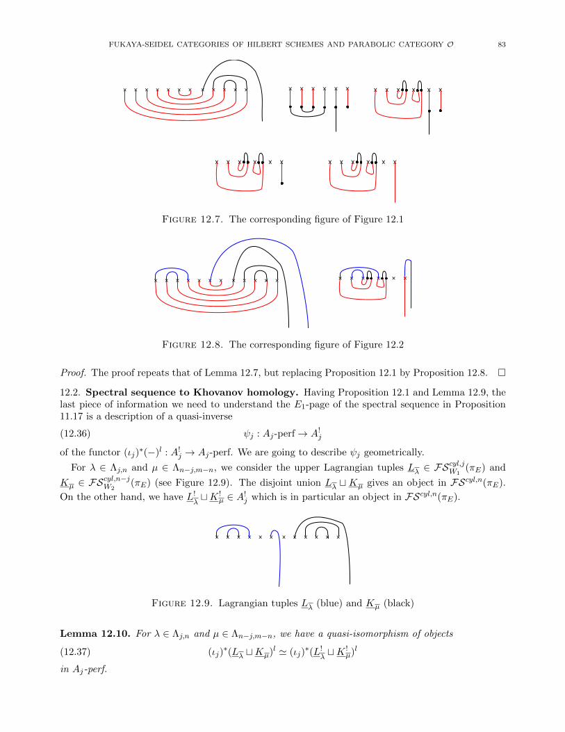
FUKAYA-SEIDEL CATEGORIES OF HILBERT SCHEMES AND PARABOLIC CATEGORY O 83
x x x x x x x x x x x x x x x x x x x x x x x x
x x x x x x x x x x x x
Figure 12.7. The corresponding figure of Figure 12.1
x x x x x x x x x x x x x x x x x x
Figure 12.8. The corresponding figure of Figure 12.2
Proof. The proof repeats that of Lemma 12.7, but replacing Proposition 12.1 by Proposition 12.8.
12.2. Spectral sequence to Khovanov homology. Having Proposition 12.1 and Lemma 12.9, thelast piece of information we need to understand the E1-page of the spectral sequence in Proposition11.17 is a description of a quasi-inverse
ψj : Aj-perf→ A!j(12.36)
of the functor (ιj)∗(−)l : A!
j → Aj-perf. We are going to describe ψj geometrically.
For λ ∈ Λj,n and µ ∈ Λn−j,m−n, we consider the upper Lagrangian tuples Lλ ∈ FScyl,jW1
(πE) and
Kµ ∈ FScyl,n−jW2
(πE) (see Figure 12.9). The disjoint union Lλ t Kµ gives an object in FScyl,n(πE).
On the other hand, we have L!λtK !
µ ∈ A!j which is in particular an object in FScyl,n(πE).
x x x x x x x x x x x x
Figure 12.9. Lagrangian tuples Lλ (blue) and Kµ (black)
Lemma 12.10. For λ ∈ Λj,n and µ ∈ Λn−j,m−n, we have a quasi-isomorphism of objects
(ιj)∗(Lλ tKµ)l ' (ιj)
∗(L!λtK !
µ)l(12.37)
in Aj-perf.

84 CHEUK YU MAK AND IVAN SMITH
Proof. For any object Lλ′ tKµ′ ∈ Aj , there is an obvious isomorphism (see Figure 12.10)
CF (Lλ tKµ, Lλ′ tKµ′) = CF (Lλ, Lλ′)⊗ CF (Kµ,Kµ′)
= CF (L!λ, Lλ′)⊗ CF (K !
µ,Kµ′)
= CF (L!λtK !
µ, Lλ′ tKµ′)
Moreover, when X0, . . . , Xd ∈ Aj , for a careful choice of Floer data, one can actually make the A∞structural maps
CF (Xd−1, Xd)× . . . CF (X0, X1)× CF (Lλ tKµ, X0)→ CF (Lλ tKµ, Xd)(12.38)
CF (Xd−1, Xd)× . . . CF (X0, X1)× CF (L!λtK !
µ, X0)→ CF (Lλ tKµ, Xd)(12.39)
completely coincide. It implies the result.
x x x x x x x x x x x x x x x x x x x x x x x x
Figure 12.10. Floer cochain CF (L!λtK !
µ, Lλ′ tKµ′) (left) and CF (Lλ tKµ, Lλ′ tKµ′) (right). The intersection between the positive wrapping of Lλ and Kµ′ cannot
contribute generator to CF (Lλ tKµ, Lλ′ tKµ′) so the Floer cochain splits.
Remark 12.11. By taking morphisms with an appropriate object in Ai for i 6= j, one can see that(Lλ tKµ)l is not quasi-isomorphic to (L!
λtK !
µ)l.
By Lemma 12.10, we know that the quasi-inverse ψj is given, on the object level, by
ψj : (ιj)∗(Lλ tKµ)l 7→ L!
λtK !
µ(12.40)
A further inspection of the proof of Lemma 12.10 shows that the quasi-isomorphism (12.37) is functorialwhen we vary λ ∈ Λj,n and µ ∈ Λn−j,m−n. Together with the fact that Lλ tKµ is quasi-isomorphic to
Lλ tKµ in FScyl,n(πE) (so the former can be regarded as an object in Aj), we have a commutative
diagram
Aj Kj,n ×Kn−j,n A!j
Aj-perf
'
(−)l
'
(ιj)∗(−)l
where the horizontal isomorphisms are the ones in (11.5), (11.9), which in particular send LλtKµ ∈ Ajto L!
λ tK !µ ∈ A!
j . This implies that ψj sits inside the commutative diagram
Aj Kj,n ×Kn−j,n A!j
Aj-perf
'
(−)l
'
ψj

FUKAYA-SEIDEL CATEGORIES OF HILBERT SCHEMES AND PARABOLIC CATEGORY O 85
Proof of Theorem 1.9. By Proposition 11.17, we have a spectral sequence to Kh(κ(β)) from
⊕nj=0H((ι!j)∗(φβ(Lhs)
r)⊗A!jψj (ιj)
∗(Llhs))(12.41)
By Proposition 12.1, Lemma 12.9 and the commutative diagram above, we have, up to grading shift,
H((ι!j)∗(φβ(Lhs)
r)⊗A!jψj (ιj)
∗(Llhs)) = H(P(j)β ⊗Kj,n−Kj,n ∆Kj,n)(12.42)
= HH∗(Kj,n, P(j)β )(12.43)
which is what we want.
Appendix A. Non-formality of standard modules/thimbles
Here we explain that the endomorphism algebra of the Lefschetz thimbles in FS(πn,m) may benon-formal when n > 1. The non-formality follows rather directly from the minimal model computedin the thesis of Klamt [27]. Since this is not required for our main results, our treatment is somewhatbrief.
When (n,m) = (1,m) the algebra is known to be formal; by duality, the same holds when n = m−1.On the other hand, if n > 1 and (n,m) 6= (m− 1,m), the algebra associated to (n,m) = (2, 4) occursas an A∞-subalgebra of the algebra associated to (n,m). It therefore suffices to consider the case(n,m) = (2, 4). In that case, there are six Lefschetz thimbles (up to grading shift). We denote them
by P (4|3), P (4|2), P (4|1), P (3|2), P (3|1) and P (2|1), where P (n|m) corresponds to T 1,2,3,4\n,m.The cohomological algebra is given by the following quiver with relations, by Proposition 10.1 and
[27, Section 5.2.8, 5.2.9].
P (4|3)
P (4|2) P (3|2)
P (4|1) P (3|1) P (2|1)
F(4|3)(4|2)
Id(4|3)(4|2)
K(4|3)(2|1)
G(4|3)(2|1)
F(4|2)(4|1)
Id(4|2)(4|1)
F(4|2)(3|2)
Id(4|2)(3|2)
F(3|2)(3|1)
Id(3|2)(3|1)
F(4|1)(3|1)
Id(4|1)(3|1)
F(3|1)(2|1)
Id(3|1)(2|1)
The subscript and superscript of the name of the arrow indicate the target and the source of the
arrow, respectively. The definition of Id(k|l)(a|b), F
(k|l)(a|b) , F
(k|l)(a|b) , G
(k|l)(a|b), K
(k|l)(a|b) for various k, l, a, b can be
found in Theorem 5.16, 5.17, 5.18 and 5.19 in [27]. The complete list of relations of the product
structure can be found in [27, Table 5.25]. For example, F(4|1)(2|1) = Id
(3|1)(2|1)F
(4|1)(3|1) and F
(4|2)(4|1)F
(4|3)(4|2) = 0.
We remark that J(k|l)(a|b) in the table is defined in Theorem 5.26 and J
(4|2)(3|1) equals to F
(3|2)(3|1) F
(4|2)(3|2) and
F(4|1)(3|1)F
(4|2)(4|1) up to sign. Moreover, the dimension of Ext(P (k|l), P (a|b)) can be found in [27, Section
5.2.6].For the A∞ structure, Klamt computed a minimal model with µ3 6= 0 but µd = 0 for d > 3. The
list of non-zero µ3 is given in [27, Table 8.4].
Lemma A.1. When (n,m) = (2, 4), the endomorphism algebra of Lefschetz thimbles is not formal.
Proof. Let B be the A∞ endomorphism algebra of Lefschetz thimbles and B := H(B) be the underlyingcohomological algebra. If B were formal, then the µ3 of the minimal model Klamt found would definethe zero class in HH3(B,B[−1]). It means that µ3 = dCCτ for some τ ∈ CC2(B,B[−1]), where dCCis the Hochschild differential.
From [27, Table 8.4], we have
µ3(F(4|1)(2|1) , F
(4|2)(4|1) , F
(4|3)(4|2) ) = ±K(4|3)
(2|1)(A.1)

86 CHEUK YU MAK AND IVAN SMITH
On the other hand, up to sign,
dCCτ(F(4|1)(2|1) , F
(4|2)(4|1) , F
(4|3)(4|2) )
=F(4|1)(2|1) τ(F
(4|2)(4|1) , F
(4|3)(4|2) ) + τ(F
(4|1)(2|1) , F
(4|2)(4|1) )F
(4|3)(4|2) + τ(F
(4|1)(2|1)F
(4|2)(4|1) , F
(4|3)(4|2) ) + τ(F
(4|1)(2|1) , F
(4|2)(4|1)F
(4|3)(4|2) )(A.2)
By [27, Table 5.25], we have F(4|1)(2|1)F
(4|2)(4|1) = F
(4|2)(4|1)F
(4|3)(4|2) = 0 so the last two terms of (A.2) vanish.
One can check from [27, Section 5.2.6] that the dimension of Ext(P (2|1), P (4|3)) is 4 and it is
generated by Id(4|3)(2|1), F
(4|3)(2|1) = F
(4|3)(2|1) , G
(4|3)(2|1) and K
(4|3)(2|1) . On the other hand, one can check from [27,
Table 5.25] that for any a ∈ Ext(P (4|1), P (4|3)) and b ∈ Ext(P (2|1), P (4|2)), the sum F(4|1)(2|1) a+bF
(4|3)(4|2)
lie in the subspace spanned by F(4|3)(2|1) . Therefore, K
(4|3)(2|1) cannot be written as the sum of the first
two terms of (A.2) so it does not equal to dCCτ(F(4|1)(2|1) , F
(4|2)(4|1) , F
(4|3)(4|2) ) for any τ in CC2(B,B[−1]).
Contradiction and the result follows.
Remark A.2. Lemma A.1 shows that the strategy from Section 9 cannot be used to prove that thecollection of thimbles is formal. In other words, the cohomological algebra of the thimbles is notcompatible with the existence of such a consistent choice of equivariant structure. It seems hard topinpoint why one would expect the collection of Lagrangians Lλλ∈Λn,m to be better in this respect.
References
[1] Mohammed Abouzaid and Ivan Smith. The symplectic arc algebra is formal. Duke Math. J., 165(6):985–1060, 2016.[2] Mohammed Abouzaid and Ivan Smith. Khovanov homology from Floer cohomology. J. Amer. Math. Soc., 32(1):1–79,
2019.[3] Lino Amorim. Tensor product of filtered A∞-algebras. J. Pure. Appl. Algebra, 220:3984–4016, 2016.[4] Marta M. Asaeda, Jozef H. Przytycki, and Adam S. Sikora. Categorification of the Kauffman bracket skein module
of I-bundles over surfaces. Algebr. Geom. Topol., 4:1177–1210, 2004.[5] Denis Auroux. Fukaya categories of symmetric products and bordered Heegaard-Floer homology. J. Gokova Geom.
Topol. GGT, 4:1–54, 2010.[6] Denis Auroux, J. Elisenda Grigsby, and Stephan M. Wehrli. Sutured Khovanov homology, Hochschild homology, and
the Ozsvath-Szabo spectral sequence. Trans. Amer. Math. Soc., 367(10):7103–7131, 2015.[7] A. Beilinson, R. Bezrukavnikov, and I. Mirkovic. Tilting exercises. Mosc. Math. J., 4(3):547–557, 782, 2004.[8] Anna Beliakova, Krzysztof K. Putyra, and Stephan M. Wehrli. Quantum link homology via trace functor I. Invent.
Math., 215(2):383–492, 2019.[9] Agnieszka Bodzenta and Julian Kulshammer. Ringel duality as an instance of Koszul duality. J. Algebra, 506:129–187,
2018.[10] Tom Braden. Perverse sheaves on Grassmannians. Canad. J. Math., 54(3):493–532, 2002.[11] Tom Braden, Anthony Licata, Nicholas Proudfoot, and Ben Webster. Quantizations of conical symplectic resolutions
II: category O and symplectic duality. Asterisque, (384):75–179, 2016. with an appendix by I. Losev.[12] Jonathan Brundan and Catharina Stroppel. Highest weight categories arising from Khovanov’s diagram algebra. II.
Koszulity. Transform. Groups, 15(1):1–45, 2010.[13] Jonathan Brundan and Catharina Stroppel. Highest weight categories arising from Khovanov’s diagram algebra I:
cellularity. Mosc. Math. J., 11(4):685–722, 821–822, 2011.[14] Neil Chriss and Victor Ginzburg. Representation theory and complex geometry. Birkhauser, 1997.[15] Kai Cieliebak and Klaus Mohnke. Symplectic hypersurfaces and transversality in Gromov-Witten theory. J. Sym-
plectic Geom., 5(3):281–356, 2007.[16] Kevin Costello. Higher genus Gromov-Witten invariants as genus zero invariants of symmetric products. Ann. of
Math. (2), 164(2):561–601, 2006.[17] Simon Donaldson and Ivan Smith. Lefschetz pencils and the canonical class for symplectic four-manifolds. Topology,
42(4):743–785, 2003.[18] Tolga Etgu and YankıLekili. Koszul duality patterns in Floer theory. Geom. Topol., 21(6):3313–3389, 2017.[19] Jonathan David Evans. Symplectic mapping class groups of some Stein and rational surfaces. J. Symplectic Geom.,
9(1):45–82, 2011.[20] Kenji Fukaya, Yong-Geun Oh, Hiroshi Ohta, Hiroshi and Kaoru Ono. Lagrangian intersection Floer theory: anom-
aly and obstruction. Part II. AMS/IP Studies in Advanced Mathematics, 46.2. American Mathematical Society,Providence, RI; International Press, Somerville, MA, 2009.

FUKAYA-SEIDEL CATEGORIES OF HILBERT SCHEMES AND PARABOLIC CATEGORY O 87
[21] J. Elisenda Grigsby, Anthony M. Licata, and Stephan M. Wehrli. Annular Khovanov homology and knotted Schur-Weyl representations. Compos. Math., 154(3):459–502, 2018.
[22] Andrew Hanlon. Monodromy of monomially admissible Fukaya-Seidel categories mirror to toric varieties.arXiv:1809.06001, 2018.
[23] D. Huybrechts. Fourier-Mukai transforms in algebraic geometry. Oxford Mathematical Monographs. The ClarendonPress, Oxford University Press, Oxford, 2006.
[24] Mikhail Khovanov. A categorification of the Jones polynomial. Duke Math. J., 101(3):359–426, 2000.[25] Mikhail Khovanov. A functor-valued invariant of tangles. Algebr. Geom. Topol., 2:665–741, 2002.[26] Mikhail Khovanov and Paul Seidel. Quivers, Floer cohomology, and braid group actions. J. Amer. Math. Soc.,
15(1):203–271, 2002.[27] Angela Klamt. A∞-structures on the algebra of extensions of Verma modules in the parabolic category O.
arXiv:1104.0102, 2011.[28] Alexander Kuznetsov. Hochschild homology and semiorthogonal decompositions. arXiv:0904.4330, 2009.[29] Robert Lipshitz. A cylindrical reformulation of Heegaard Floer homology. Geom. Topol., 10:955–1096, 2006.[30] Robert Lipshitz, Peter S. Ozsvath, and Dylan P. Thurston. Bimodules in bordered Heegaard Floer homology. Geom.
Topol., 19(2):525–724, 2015.[31] Ciprian Manolescu. Nilpotent slices, Hilbert schemes, and the Jones polynomial. Duke Math. J., 132(2):311–369,
2006.[32] Ciprian Manolescu. Link homology theories from symplectic geometry. Adv. Math., 211(1):363–416, 2007.[33] Maksim Maydanskiy and Paul Seidel. Lefschetz fibrations and exotic symplectic structures on cotangent bundles of
spheres. J. Topol., 3(1):157–180, 2010.[34] Dusa McDuff and Dietmar Salamon. J-holomorphic curves and symplectic topology. American Mathematical Society
Colloquium Publications. American Mathematical Society, Providence, RI, 2004.[35] Peter Ozsvath and Zoltan Szabo. Holomorphic disks and topological invariants for closed three-manifolds. Ann. of
Math. (2), 159(3):1027–1158, 2004.[36] Tim Perutz. Lagrangian matching invariants for fibred four-manifolds. I. Geom. Topol., 11:759–828, 2007.[37] Tim Perutz. Lagrangian matching invariants for fibred four-manifolds. II. Geom. Topol., 12(3):1461–1542, 2008.[38] Marcin Pozniak Floer homology, Novikov rings and clean intersections. Northern California Symplectic Geometry
Seminar, Amer. Math. Soc. Transl. Ser. 2, Amer. Math. Soc., Providence, RI, vol. 196, 119–181, 1999.[39] Lawrence P. Roberts. On knot Floer homology in double branched covers. Geom. Topol., 17(1):413–467, 2013.[40] Paul Seidel. Fukaya categories and Picard-Lefschetz theory. Zurich Lectures in Advanced Mathematics. European
Mathematical Society (EMS), Zurich, 2008.[41] Paul Seidel. Symplectic homology as Hochschild homology. In Algebraic geometry—Seattle 2005. Part 1, volume 80
of Proc. Sympos. Pure Math., pages 415–434. Amer. Math. Soc., Providence, RI, 2009.[42] Paul Seidel. Fukaya A∞-structures associated to Lefschetz fibrations. I. J. Symplectic Geom., 10(3):325–388, 2012.[43] Paul Seidel. Fukaya A∞-structures associated to Lefschetz fibrations. II 1/2. Adv. Theor. Math. Phys., 20(4):883–944,
2016.[44] Paul Seidel. Fukaya A∞-structures associated to Lefschetz fibrations. II. In Algebra, geometry, and physics in the
21st century, volume 324 of Progr. Math., pages 295–364. Birkhauser/Springer, Cham, 2017.[45] Paul Seidel. Fukaya A∞-structures associated to Lefschetz fibrations. IV. arXiv:1709.06018, 2017.[46] Paul Seidel. Fukaya A∞-structures associated to Lefschetz fibrations. IV 1/2. arXiv:1802.09461, 2018.[47] Paul Seidel and Ivan Smith. A link invariant from the symplectic geometry of nilpotent slices. Duke Math. J.,
134(3):453–514, 2006.[48] Kyler Siegel Squared Dehn twists and deformed symplectic invariants. arXiv:1609.08545, 2016.[49] Nick Sheridan. On the homological mirror symmetry conjecture for pairs of pants. J. Differential Geom., 89(2):271–
367, 2011.[50] Peter Slodowy. Simple singularities and simple algebraic groups, volume 815 of Lecture Notes in Mathematics.
Springer, Berlin, 1980.[51] Catharina Stroppel. Parabolic category O, perverse sheaves on Grassmannians, Springer fibres and Khovanov ho-
mology. Compos. Math., 145(4):954–992, 2009.[52] Claire Voisin. On the punctual Hilbert scheme of a symplectic fourfold. In Symposium in Honor of C. H. Clemens
(Salt Lake City, UT, 2000), volume 312 of Contemp. Math., pages 265–289. Amer. Math. Soc., Providence, RI, 2002.[53] Maxim Vybornov. Perverse sheaves, Koszul IC-modules, and the quiver for the category O. Invent. Math., 167(1):19–
46, 2007.
Centre for Mathematical Sciences, University of Cambridge, CB3 0WB, UK
E-mail address: [email protected]
Centre for Mathematical Sciences, University of Cambridge, CB3 0WB, UK
E-mail address: [email protected]