ftir spectroscopic prediction of klason and acid soluble ... · with the klason lignin (gravimetric...

351

www.metla.fi/silvafennica · ISSN 0037-5330The Finnish Society of Forest Science · The Finnish Forest Research Institute

FTIR Spectroscopic Prediction of Klason and Acid Soluble Lignin Variation in Norway Spruce Cutting Clones

Sanni Raiskila, Minna Pulkkinen, Tapio Laakso, Kurt Fagerstedt, Mia Löija, Riitta Mahlberg, Leena Paajanen, Anne-Christine Ritschkoff and Pekka Saranpää

Raiskila, S., Pulkkinen, M., Laakso, T., Fagerstedt, K., Löija, M., Mahlberg, R., Paajanen, L., Ritschkoff, A.-C. & Saranpää, P. 2007. FTIR spectroscopic prediction of Klason and acid soluble lignin variation in Norway spruce cutting clones. Silva Fennica 41(2): 351–371.

Our purpose was to develop a FTIR spectroscopic method to be used to determine the lignin content in a large number of samples and to apply this method studying variation in sapwood and heartwood lignin content between three fast-growing cutting clones grown in three sites. Models were estimated with 18 samples and tested with 6 samples for which the Klason lignin + acid soluble lignin content had been determined. Altogether 272 candidate models were built with all-subset regressions from the principal components estimated from differ-ently treated transmission spectra of the samples; the spectra were recorded on KBr pellets of sieved and unsieved unextracted wood powder and subjected to four different preprocessings and two different wavenumber selection schemes. The final model showed an adequate fit in the estimation data (R2 = 0.74) as well as a good prediction performance in the test data (R2

P = 0.90). This model was based on the wavenumber range of 1850–500 cm–1 of the line-subtraction-normalised spectra recorded from sieved samples. The model was used to predict lignin content in 64 samples of the same material. One of the clones had a slightly lower sapwood lignin content than the two other clones. The fertile growing site with fast growing trees showed slightly higher sapwood lignin content compared with the other two sites. The model was also used to predict the lignin content in the earlywood of 45 individual annual rings. Variation between individual stems and between annual rings was found to be large. No correlation was found between the lignin content and density of earlywood.

Keywords FTIR, lignin, Norway spruce, PCR, principal component regressionAuthors’ addresses Saranpää, Raiskila and Laakso, Finnish Forest Research Institute, Vantaa Research Unit, P.O. Box 18, FI-01301 Vantaa, Finland; Pulkkinen, Department of Forest Ecology, P.O. Box 27, FI-00014 University of Helsinki, Finland; Fagerstedt, Department of Biological and Environmental Sciences, Plant Biology, P.O. Box 65, FI-00014 University of Helsinki, Finland; Ritschkoff, Löija, Mahlberg and Paajanen, VTT Building and Transport, P.O. Box 1806, FI-02044 VTT, Finland E-mail [email protected] 26 July 2006 Revised 22 January 2007 Accepted 13 March 2007Available at http://www.metla.fi/silvafennica/full/sf41/sf412351.pdf

Silva Fennica 41(2) research articles

352

Silva Fennica 41(2), 2007 research articles

1 IntroductionThe conifer cell wall consists of 40–50% cellu-lose, 20–35% hemicellulose and 15–35% lignin (Panshin and deZeeuw 1980, Sjöström 1993, Walker 1993). In the stem wood of Norway spruce the mean lignin content (gravimetric lignin + acid soluble lignin) has been reported to be 28.9% with standard deviation of 0.8% (Anttonen et al. 2002, Anttonen, personal communication). The variation of lignin content in wood raw mate-rial causes problems to wood-utilizing industry, which endeavours to assure a uniform quality of the end products. On the other hand, the natural genetic variation in trees provides an opportunity to select individuals with desirable lignin contents for breeding. So far, however, the genetic varia-tion in lignin content or composition in trees has been studied very little.

The lignin content has traditionally been deter-mined by wet chemical methods e.g. with the acetyl bromide method (spectrophotometric method) suitable for a small amount of sample (Iiyama and Wallis 1988, Hatfield et al. 1999, Fukushima and Hatfield 2001, Hatfield and Fukushima 2005) and with the Klason lignin (gravimetric method) and acid soluble lignin (spectrophotometric method) measurement (Dence 1992) suitable for a large amount of sample. In the first method the ground extracted wood is dissolved in acetyl bromide in acetic acid containing perchloric acid and in the latter methods degraded with sulphuric acid (Iiyama and Wallis 1988). The extraction is often, e.g. with the Soxhlet method, slow and consumes a large amount of organic solvent. Hence, it is unfeasible for large sets of samples. A rapid and reproducible method for screening of lignin con-tent, as well as other cell wall properties, would thus be welcome to practical wood use and tree breeding purposes.

Transmission or diffuse reflectance spectra in the mid infrared or near infrared regions (NIR) are fast and relatively easy to measure and have been shown to provide reliable information on the chemical properties of biological materials. The KBr transmission technique is the most common tool for the quantitative estimation of lignin and suitable for routine work (Faix 1992). The diffuse reflectance infrared Fourier transform (DRIFT) method is suitable for a wood surface investiga-

tion and the lignin evaluation in wood, though its reproducibility is considered to be poor (Faix 1992). Absorption bands of spectrum represent vibration frequencies, which are characteristic of covalent bonds or functional groups and a whole molecule. The problem from the lignin model-ling point of view is that many of the chemical components in wood contribute to the intensities at all or a large part of the wavenumbers, and that few wavenumber regions or bands, if any, thus reflect purely lignin (Ferraz et al. 2000, Costa e Silva et al. 1999); specifically, the aromatic signal intensities are low in comparison with the more polar polysaccharides. Consequently, it would seem prudent to base lignin content modelling on the intensity information on the whole spectrum. This is likely to result in a dimensionality prob-lem, as a spectrum typically consists of intensities at some thousands of wavenumbers but not more than some dozens or hundreds wood samples can realistically be expected to be available for modelling.

In earlier studies, the relation between lignin content of a wood sample and a Fourier transform infrared (FTIR) spectra measured on it has been quite successfully modelled using linear regres-sion in Eucalyptus globulus (Rodrigues et al. 1998), principal component regression (PCR) in Picea sitchensis and biodegraded Pinus radiata (Costa e Silva et al. 1999, Ferraz et al. 2000), par-tial least squares (PLS-1) in Pinus radiata (Meder et al. 1999), and projection to latent structures (PLS-2; lignin modelled simultaneously with glucan and polyoses) in biodegraded Eucalyp-tus globulus and Pinus radiata (Ferraz et al. 2000). The models have been built with a collec-tion of individual wavenumbers or wavenumber regions or the whole spectrum as the input; the dimension reduction has then been tackled with a theoretically or empirically motivated selection of individual wavenumbers, or with principal component analysis (PCA), or, as in PLS-1 and PLS-2 methods, with a method resembling PCA where the components are formed by maximis-ing not their variances but their covariances with the lignin content. The work by Gierlinger et al. (2002), although not dealing with lignin and FTIR but modelling heartwood extractives in Larix sp. with PLS models based on FTNIR spectra, sets a good example in coping with the various aspects

353

Raiskila et al. FTIR Spectroscopic Prediction of Klason and Acid Soluble Lignin Variation in Norway Spruce Cutting Clones

of sample preparation, spectrum preprocessing, wavenumber selection as well as model valida-tion and evaluation that one is likely to encounter is this kind of modelling work. However, as far as we know, no such work has been done on Norway spruce. Also, although many articles have been written on the building of the statistical models, very few if any report the actual use of the obtained models for the purposes (e.g. screening) to which they were intended.

The purpose of our work was to develop a method based on FTIR spectra to determine the relative total lignin content of clonal Norway spruce samples and to use the method to study lignin variation in a large number of samples of similar kind. The aim was to replace the combina-tion of three wet chemical methods (extraction, Klason lignin and acid soluble lignin determina-tion) with one FTIR spectroscopic method, where the total lignin content is predicted in the small amount of powdered unextracted wood sample. This paper describes the building of an empirical lignin content model by using all-subset princi-pal component regression; with the model, the percentage of dry mass of total lignin in a wood sample may be predicted by the FTIR spectrum measured on it. The key feature of the model building was that the selection of the final model was based equally on its fit in the estimation data and on its prediction performance in the test data. The paper also reports the application of the model to predict the lignin content variation in a large number of samples taken from the same three Norway spruce cutting clones planted on the same three sites of different fertility and climate from which the model was built.

2 Material and Methods

2.1 Material

Disks of wood were sawn at breast height (1.3 m) from the stems of 44 trees representing three dif-ferent Norway spruce (Picea abies [L.] Karst.) cutting clones (A, B, C) growing at three different sites in Finland: Loppi (60°37Ń 24°26É), Imatra (61°08Ń 28°48É) and Kangasniemi (61°57Ń 26°41É). The trees were 26, 28 and 24 years old

at the time of felling. Samples (about 5 g) were taken from annual rings 3–6 in the heartwood and from three annual rings (rings between 13 and 22) in the middle of sapwood area. The distribution of the samples in different site-clone combinations is shown in Table 1. In addition, samples were taken from earlywood of 45 individual annual rings from 9 trees (5 samples per tree, 3 trees per each of the three clones) grown in one site (Loppi). Trees with the highest, average and slow-est growth rate were chosen from each of the three clones. Annual rings with high and low peaks of weight density were further chosen in order to maximise density variation. The samples were taken avoiding knots and compression wood. The Norway spruce clones and their growth rate, weight density, mechanical strength properties and lignin modification experiments are described in Raiskila et al. 2006a, 2006b.

2.2 Klason Lignin and Acid Soluble Lignin Measurement

For model estimation and model testing, the relative total lignin (Klason lignin + acid solu-ble lignin) content was measured in duplicate for the sapwood and heartwood samples of 12 stems (24 samples) representing the three dif-ferent clones growing in the three different sites (Table 1). Wood samples were ground frozen with a blade-mill (Polymix PX-A10). The dry solids content of the milled wood samples was determined at 103 °C. The samples of air-dried wood powders (3 g) were extracted with acetone, ethanol and water using a Soxhlet apparatus for 6 hours with each solvent separately (modified KCL 1982). After evaporation of the solvents the residues were dried at 103 °C, allowed to cool in a desiccator and then weighed. The amount of acid insoluble lignin was determined by the Klason method (KCL 1982, Dence 1992). The samples of the extracted wood powders (300 mg) were treated with 3 cm3 of 72% sulfuric acid in an ultrasonic bath for 1 hour. The mixtures were diluted with about 82 cm3 portions of water and autoclaved at 125 °C for 1 hour. The precipitates were collected with sintered glasses (4G) by suc-tion filtration and washed with water. The sinters with the acid insoluble lignin (Klason lignin)

354


were dried at 103 °C, cooled in the desiccator and weighed. In order to determine the amount of acid soluble lignin the filtrates were diluted with water to 250 cm3. Absorption of the acid solutions with the dissolved lignin was measured at 203 nm using sulfuric acid of the same concentration as a blank (KCL 1982). The absorbance readings were obtained with a Shimadzu UV-2401 PC UV-VIS Recording spectrophotometer. The relative total lignin (Klason lignin + acid soluble lignin) con-tent was calculated from the unextracted wood as follows: Klason lignin % = p × (100 – u) / m, in which p = precipitate [g], u = extractives [%] and

m = calculated dry weight of extracted sample [g]. The acid soluble lignin content was calculated using a lignin absorptivity of 128 l g–1 cm–1 and corrected because of the absorption of carbohy-drates according to a procedure of KCL (1982). The relative total lignin content of each sample was determined as the mean of the duplicate measurements; this is referred to as the measured lignin content of the sample. The variation of the measured lignin contents in the model estima-tion and model testing data sets is summarised in Table 2.

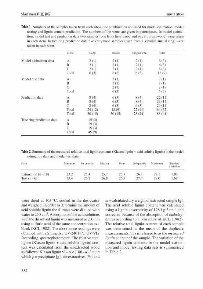
Table 1. Numbers of the samples taken from each site-clone combination and used for model estimation, model testing and lignin content prediction. The numbers of the stems are given in parentheses. In model estima-tion, model test and prediction data two samples (one from heartwood and one from sapwood) were taken in each stem. In tree ring prediction data five earlywood samples (each from a separate annual ring) were taken in each stem.

Clone Loppi Imatra Kangasniemi Total

Model estimation data A 2 (1) 2 (1) 2 (1) 6 (3) B 2 (1) 2 (1) 2 (1) 6 (3) C 2 (1) 2 (1) 2 (1) 6 (3) Total 6 (3) 6 (3) 6 (3) 18 (9)

Model test data A 2 (1) 2 (1) B 2 (1) 2 (1) C 2 (1) 2 (1) Total 6 (3) 6 (3)

Prediction data A 8 (4) 6 (3) 8 (4) 22 (11) B 8 (4) 6 (3) 8 (4) 22 (11) C 8 (4) 6 (3) 6 (3) 20 (11) Total 24 (12) 18 (9) 22 (11) 64 (32) Total 30 (15) 30 (15) 28 (24) 88 (44)

Tree ring prediction data A 15 (3) B 15 (3) C 15 (3) Total 45 (9)

Table 2. Summary of the measured relative total lignin contents (Klason lignin + acid soluble lignin) in the model estimation data and model test data.

Data Minimum 1st quartile Median Mean 3rd quartile Maximum Standard deviation

Estimation (n = 18) 23.2 25.4 25.7 25.7 26.1 28.1 1.03 Test (n = 6) 23.4 26.2 26.8 26.5 27.7 28.0 1.68

355


2.3 FTIR Analysis

For model estimation and model testing, FTIR analysis was performed in triplicate on the same 24 samples of 12 stems for which the relative total lignin (Klason lignin + acid soluble lignin) content was measured with the wet chemical methods. For lignin content prediction, single spectra were recorded on the heartwood and sap-wood samples of the rest 32 stems (64 samples; Table 1) and in addition to this double spectra on the earlywood samples of annual rings (45 samples) from the 9 stems collected from one site (Loppi). Wood samples were ground frozen with a blade-mill (Polymix PX-A10), and half of the unextracted finely ground wood was passed through a sieve with hole size of 0.125 mm (see Faix and Böttcher 1992). Subsamples of 3.00–3.04 mg of sieved and unsieved wood powder were added to 300.0–301.0 mg of dry KBr in test tubes. The samples were dried at 60 °C for 2 hours, then cooled in a desiccator and mixed with a test tube mixer. The mixtures were pressed (112 bar / 2 min) into discs with a diameter of 13 mm using a hydraulic press (Perkin Elmer, Hydraulische Presse) equipped with a vacuum pump. FTIR spectra were then recorded from the KBr tablets of the sieved and unsieved samples (3 tablets per sample for model estimation and test-ing, 1 tablet per sample or 2 tablets per earlywood samples for lignin content prediction) on a Perkin Elmer System 2000 FT-IR spectrometer (software version 4.0) equipped with a MIRTGS detector with a resolution of 4 cm–1 using the transmission technique. Altogether 16 scans were accumulated from each sample. Data were acquired in the wav-enumber range of 4000–500 cm–1 (wavelength range of 2500–20 000 nm).

2.4 Principal Component Regression Modelling

Principal component regression (PCR), instead of the also commonly used partial least squares (PLS), was chosen as the modelling approach because it straightforwardly follows the standard statistical theory of linear models (as to estima-tion, testing and prediction; see e.g. Jolliffe 2002) and because it, unlike PLS, is easy to carry out

with any general statistical or matrix computation software. In general, PCR and PLS have been found in practice to give comparable results (Næs et al. 2002).

As already mentioned, the 24 samples from the12 trees for building lignin content models were divided into two sets: model estimation data consisted of 18 samples from 9 trees, each tree representing one of the three clones growing in one of the three sites (Table 1), whereas model test data comprised 6 samples from 3 trees, each tree representing one of the three clones growing in one site (Imatra; Table 1).

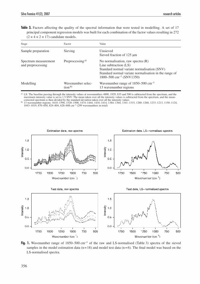
Three different preprocessing methods (nor-malisations) were applied to the spectra recorded on the sieved and unsieved samples (Table 3). The normalisations were performed on each of the three repeated spectrum measurements of a sample, and the final normalised spectrum was then the pointwise average of these nor-malised replicates. Of the whole wavenumber range (4000–500 cm–1), only the subrange of 1850–500 cm–1 known to encompass lignin-related information (Hergert 1971) was eventu-ally employed in the modelling. Alternatively, to diminish the effect of lignin-unrelated variation in intensity values, the modelling was performed on 13 subjectively selected wavenumber regions con-taining 299 wavenumbers (Table 3), the choice of which was based on chemical knowledge (Hergert 1971) and previous empirical work (e.g. Rod-rigues et al. 1998, Costa e Silva et al. 1999). In Fig. 1, the wavenumber range of 1850–500 cm–1 of the raw and LS-normalised spectra of the sieved samples in the model estimation data and model test data are shown.

PCR was carried out separately for each com-bination of the sieving, normalisation and wav-enumber selection factor values (Table 3). There were altogether 16 factor value combinations resulting from two sieving methods, four nor-malisations (raw spectra included) and two wav-enumber selection schemes. The first stage of PCR, the principal component analysis (PCA) for dimension reduction, was performed on the sample covariance matrix of the intensity vari-ables (intensities at wavenumbers 1850–500 cm–1 or at the 299 wavenumbers of the 13 wavenum-ber regions). The matrix was estimated from the samples in the estimation data set. The use of

356


Table 3. Factors affecting the quality of the spectral information that were tested in modelling. A set of 17 principal component regression models was built for each combination of the factor values resulting in 272 (2 × 4 × 2 × 17) candidate models.

Stage Factor Value

Sample preparation Sieving UnsievedSieved fraction of 125 µm

Spectrum measurementand preprocessing

Preprocessing a) No normalisation, raw spectra (R)Line subtraction (LS)Standard normal variate normalisation (SNV) Standard normal variate normalisation in the range of 1800–500 cm–1 (SNV1350)

Modelling Wavenumber selec-tion b)

Wavenumber range of 1850–500 cm–1

13 wavenumber regions

a) LS: The baseline passing through the intensity values at wavenumbers 4000, 1929, 835 and 500 is subtracted from the spectrum, and the maximum intensity value is set to 1.5 SNV: The mean taken over all the intensity values is subtracted from the spectrum, and the mean-corrected spectrum is then divided by the standard deviation taken over all the intensity values

b) 13 wavenumber regions: 1610–1590, 1520–1500, 1474–1444, 1434–1414, 1384–1364, 1341–1315, 1280–1260, 1233–1213, 1150–1124, 1043–1019, 870–850, 824–804, 628–608 cm–1 (299 wavenumbers in total)

Fig. 1. Wavenumber range of 1850–500 cm–1 of the raw and LS-normalised (Table 3) spectra of the sieved samples in the model estimation data (n = 18) and model test data (n = 6). The final model was based on the LS-normalised spectra.

357


the covariance matrix was justified by the fact that the observed intensities in different samples were more or less at the same measurement scale. Thus, their variances were of similar magnitude, especially after the within-spectrum normalisa-tion. Of the resulting principal components (PCs; uncorrelated linear combinations of the intensity variables), the 17 first ones accounting for a non-zero portion of the total variance of the intensity variables were retained in the analysis.

The retained PCs constituted the set of pos-sible explanatory variables in an ordinary linear model with the measured relative total lignin content as the response variable and with the usual assumptions on the additive random error term, i.e. the error terms of different observations are independent and identically normally distributed with expectation 0 and constant variance. The parameters of the all-subset regressions were esti-mated with the ordinary least squares method (OLS) in the estimation data, i.e. all the possible combinations of the 17 retained PCs were tried as explanatory variables. In each model size class p = 1, 2, …, 17, (i.e., among the models with p PCs as the explanatory variables), the model with the largest adjusted coefficient of determi-nation (R2

adj), or equivalently, with the smallest root mean square error (RMSE) was taken as a candidate model for the final model selection (for the definition of the concepts, see e.g. Weisberg 1985 and Table 4).

Note that in the parameter estimation the model assumption of mutually independent observations (samples) was clearly violated by the within-tree and within-plot dependencies of the estimation data. Such a flaw is not unusual in these kind of studies (see e.g. Meder et al. 1999), but it is usually passed without a mention. The vio-lation causes the parameter estimate variances to become underestimated and, accordingly, the related significance tests to become too optimis-tic, whereas the parameter estimates themselves are still unbiased (Weisberg 1985). This can be regarded as acceptable for a prediction model.

As we were aspiring after a model for predic-tion, the selection among the 17 × 16 = 272 candi-date models (17 models in each of the 16 factor value combinations) was based not only on the fit in the estimation data but also on the perform-ance in the leave-one-out cross-validation in the

estimation data and, most importantly, on the prediction capability in the test data. Therefore, the root mean square error of lignin content in the estimation data (RMSE), the leave-one-out cross-validation estimate of root mean square prediction error in the estimation data (RMSPECV), and the root mean square prediction error in the test data (RMSPE) were computed for each candidate model and used as the model selection criteria (for the definition of the concepts, see e.g. Weis-berg 1985 and Table 4). The criteria were plotted against the model size, and the most parsimonious models – to avoid over-fitting – with satisfying criteria values were chosen for further study. This involved 1) checking the model assump-tions (normality of residuals with Q-Q plots, vari-ance homoscedasticity of residuals with residual plots), 2) testing the significance of the parameter estimates (F-test for overall model significance, t-tests for individual parameters), 3) diagnosing the model fit (by means of plots of raw residuals, standardised residuals and studentised residu-als) and 4) studying the influence of individual observations (leverages, and changes in regres-sion coefficients, predicted values and RMSE that result from the deletion of each observation) in the customary manner (see e.g. Belsley et al.1980, Weisberg 1985). The model with the best “overall performance” was chosen as the final model to be used for lignin content prediction in this study. Modelling computations were performed with S-Plus 3.4 and R 1.9.1 software (Venables and Ripley 1997, http://www.r-project.org/).

2.5 Lignin Content Prediction

With the final model, the relative total lignin con-tent was predicted in 64 samples from 32 trees, 12 trees being taken from Loppi (4 trees per each of the three clones), 9 trees from Imatra (3 trees per each of the three clones), and 11 trees from Kangasniemi (4 trees per clones A and B, 3 trees per clone C; Table 1). To avoid extrapolation in the explanatory variables, the similarity of the normalised spectrum of each sample to the nor-malised spectra in the model estimation data was controlled with the Hotelling T2 test based on the Mahalanobis distance between the sample and the estimation data centroid in the relevant PC-

358


space (Mardia et al. 1979). All the samples with the observed p-value larger than 0.05 were taken into the prediction (i.e., the samples accepting the null hypothesis that the sample point equals the estimation data centroid in the PC-space given the normality of distribution and the common covari-ance matrix estimated with the sample covariance matrix). In addition, the relative total lignin con-tent was predicted in 45 earlywood samples (5 samples per tree) from 9 trees (3 trees per each of the three clones) from Loppi (Table 1).

A point prediction of the lignin content of a sample was obtained as the fixed part of the final model with the estimated parameter values. As usual, the PC scores used as the explanatory variable values were computed from the centered spectrum of the new sample; centering was done with the mean spectrum of the estimation data. The variance of the point prediction, the variance of the prediction error, and the 95% prediction interval based on the normality assumption were estimated in the usual manner (Weisberg 1985) using the RMSE and the inverse of the moment matrix of the model in the estimation data as well as the vector of the PC scores computed from the new sample spectrum as the input.

A Matlab macro was constructed to facilitate the use of the model for prediction. With a LS-normalised spectrum as the input, the macro out-puts the point prediction, the estimated variance of the point prediction, the estimated variance of the prediction error, and the 95% prediction interval.

2.6 Statistical Analysis of Measured and Predicted Lignin Contents

The relative total lignin content measurements (24 samples from 12 trees) obtained with the wet chemical methods and predictions (64 samples from 32 trees) obtained with the final model were pooled into one data set. Differences in the amount of lignin in these data were analysed with the one-way analysis of variance (ANOVA) using a mixed model in the SPSS for Windows program version 12.0.1. The effect of clone (A, B, C) and growth site (Loppi, Imatra, Kangasniemi) on the heartwood and sapwood lignin content was tested pairwise at p ≤ 0.05 level with a one-way

Tukey HSDa,b,c test based on the normal distri-bution. The stem was used as a random factor. Differences in the predicted relative total lignin content of earlywood (45 samples from 9 trees) obtained with the final model were analysed with the one-way ANOVA and the effect of year on the earlywood lignin content was tested pairwise at p ≤ 0.05 level with the Tukey HSD test. The results were considered at significance levels p ≤ 0.05, p ≤ 0.01 and p ≤ 0.001.

3 Results

3.1 Principal Component Regression Modelling

In Fig. 2, the model selection criteria (RMSE, RMSPECV, RMSPE) are plotted as a function of model size (the number of PCs involved) for 213 of all the 272 candidate models considered; each point represents the model with the smallest RMSE in the particular size class and factor value combination, and models of larger size and with larger RMSE than the one with the minimum RMSE in the particular factor value combination are omitted. The figure very concretely exposes the trade-off between a good fit and a decent prediction capability: large models with many PCs tended to follow the estimation data too closely and thus predicted poorly in the slightly different test data. Especially the models based on unsieved samples seemed to be prone to this over-fitting. Irrespective of the preprocessing method applied, the models based on sieved samples and continuous wavenumber range 1850–500 cm–1 showed the most balanced behaviour in terms of all the three model selection criteria, and there-fore the attention was focused on this class of 54 models.

Due to the risk of over-fitting, models with more than 7–8 PCs in the chosen model class were considered unfeasible for prediction, even though they were performing quite well also in the test data (producing RMSPEs around 1.0%; Fig. 2). The set of possible candidates was hence reduced into 32 models with less than 9 PCs in them. The statistical quality of these models was examined, and many of the models proved to be

359


decent (with adequate normality and homoscedas-ticity of residuals, signifi cant parameter estimates, “clean” residual plots etc.). The aim being a model for prediction, the role of the test data was emphasised in the fi nal selection among the statistically adequate models: the model with the clearly smallest RMSPE in the test data (Fig. 2) was chosen as the fi nal model. This decision meant dismissing several adequate models fi tting better to the estimation data but predicting worse in the test data. The Hotelling T2 test showed (p = 0.0747) that the test data, although collected from only one site (Imatra), does not signifi cantly (at 0.05 risk level) deviate from the estimation data in the 4-dimensional PC-space associated to the model (given the normality assumption and

the common estimated covariance matrix); thus the prediction error in the test data is a reasonable selection criterion when the model is intended to be applied to similar kind of data.

The fi nal model is summarised in Table 4. Note that the fi rst PC accounting for 86% of the total variance of the intensity variables in the estimation data was not included in the model, which indicates that most of the spectral varia-tion between the samples was due to chemical properties unrelated with the lignin content. The coeffi cients of the intensity variables in the 4 PCs included in the model are presented in Fig. 3. The model fi t in the estimation data and the predic-tion performance in the test data are illustrated in Fig. 4; following the common statistical terminol-

Fig. 2. Model selection criteria (RMSE, RMSPECV, RMSPE) with respect to model size (number of principal components included as the explanatory variables) in 213 of the 272 candidate models obtained with different wood powder sieving procedures, spectrum preprocessings and wavenumber selections (Table 3). RMSE is the root mean square error of lignin content in the estimation data (n = 18), RMSPECV is the leave-one-out cross-validation estimate of root mean square prediction error in the estimation data, and RMSPE is the root mean square prediction error in the test data (n = 6). Each point represents the model with the smallest RMSE in that size class. The model selected for use in prediction in this study (Table 4) is marked with a black square.

360


ogy, the lignin content obtained with the model is termed estimated lignin content for the samples in the model estimation data and predicted lignin content for the samples in the independent model test data.

The residual plots of the model (Fig. 5) reveal one deviating sample in the estimation data with a negative residual larger than 1% in absolute value and with standardised and studentised residu-als below –2. However, this heartwood sample from the clone A growing in Loppi could not be categorised as an outlier: its spectrum did not significantly differ from the centroid of the other model estimation data in the 4-dimensional PC-space, nor was its measured lignin content (25.07%) extreme. Fortunately, the leverage of the observation was low (0.146), and its removal

did not markedly influence the model parameter estimates, RMSE or the predicted lignin value.

3.2 Lignin Content Prediction

All the 64 samples from the 32 trees in the predic-tion data were accepted for the prediction, as their Mahalanobis distances from the model estimation data centroid were small enough not to result in similarity hypothesis rejection in Hotelling T2 test at 0.05 risk level. The different sites did not considerably differ from each other in terms of the distribution of the Mahalanobis distances.

As is evident from the formulae of the variance of the point prediction (which incorporates the effect of the error in the parameter estimates of

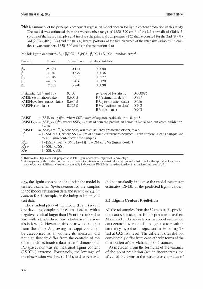
Table 4. Summary of the principal component regression model chosen for lignin content prediction in this study. The model was estimated from the wavenumber range of 1850–500 cm–1 of the LS-normalised (Table 3) spectra of the sieved samples and involves the principal components (PC) that accounted for the 2nd (8.9%), 3rd (2.0%), 4th (1.3%) and 6th (0.3%) largest portions of the total variance of the intensity variables (intensi-ties at wavenumbers 1850–500 cm–1) in the estimation data.

Model: lignin content a) = β0 + β1PC2 + β2PC3 + β3PC4 + β4PC6 + random error b)

Parameter Estimate Standard error p-value of t-statistic

β0 25.681 0.143 0.0000 β1 2.046 0.575 0.0036 β2 –3.049 1.231 0.0277 β3 –4.367 1.496 0.0120 β4 9.802 3.240 0.0098

F-statistic (df 4 and 13) 9.100 p-value of F-statistic 0.000986RMSE (estimation data) 0.606% R2 (estimation data) 0.737RMSPECV (estimation data) 0.686% R2

adj (estimation data) 0.656RMSPE (test data) 0.525% R2

CV (estimation data) 0.702 R2

P (test data) 0.903

RMSE = [SSE / (n – p)]1/2, where SSE = sum of squared residuals, n = 18, p = 5RMSPECV = [SSECV / n]1/2, where SSECV = sum of squared prediction errors in leave-one-out cross-validation,

n = 18RMSPE = [SSEP / m]1/2, where SSEP = sum of squared prediction errors, m = 6R2 = 1 – SSE / SST, where SST = sum of squared differences between lignin content in each sample and

mean lignin content over the samplesR2

adj = 1 – [SSE / (n–p)] / [SST / (n – 1)] = 1 – RMSE2 / Var(lignin content)R2

CV = 1 – SSECV / SSTR2

P = 1 – SSEP / SST

a) Relative total lignin content: proportion of total lignin of dry mass, expressed in percentageb) Assumptions on the random error needed in parameter estimation and statistical testing: normally distributed with expectation 0 and vari-

ance σ2, errors of different observations mutually independent. RMSE2 in the estimation data is an unbiased estimate of σ2.

361


Fig. 4. Relative total lignin contents estimated/predicted with the final model (Table 4) versus the measured (Klason lignin + acid soluble lignin measurement) values in the model estimation data (n = 18) and model test data (n = 6).

Fig. 3. Coefficients of the intensity variables (intensities at wavenumbers 1850–500 cm–1) in the four principal components (PC) included in the final model (Table 4); the PCs were estimated from the wavenumber range of 1850–500 cm–1 of the LS-normalised spectra of the sieved samples in the model estimation data (n = 18) (Fig. 1, Table 3).

362


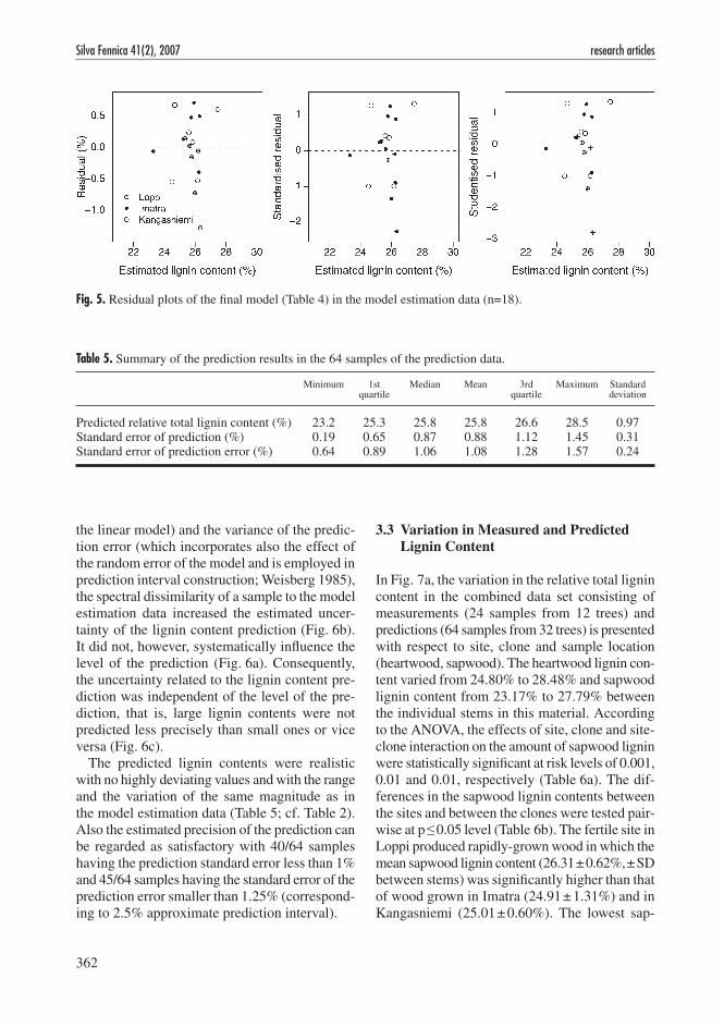
Fig. 5. Residual plots of the final model (Table 4) in the model estimation data (n=18).

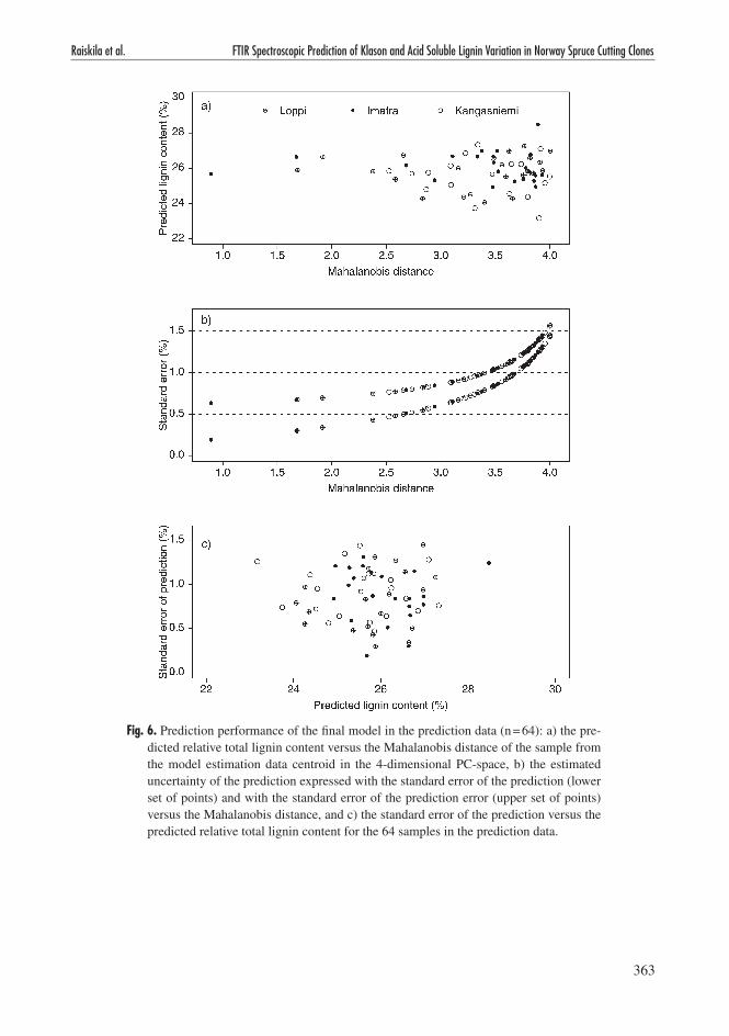
the linear model) and the variance of the predic-tion error (which incorporates also the effect of the random error of the model and is employed in prediction interval construction; Weisberg 1985), the spectral dissimilarity of a sample to the model estimation data increased the estimated uncer-tainty of the lignin content prediction (Fig. 6b). It did not, however, systematically influence the level of the prediction (Fig. 6a). Consequently, the uncertainty related to the lignin content pre-diction was independent of the level of the pre-diction, that is, large lignin contents were not predicted less precisely than small ones or vice versa (Fig. 6c).

The predicted lignin contents were realistic with no highly deviating values and with the range and the variation of the same magnitude as in the model estimation data (Table 5; cf. Table 2). Also the estimated precision of the prediction can be regarded as satisfactory with 40/64 samples having the prediction standard error less than 1% and 45/64 samples having the standard error of the prediction error smaller than 1.25% (correspond-ing to 2.5% approximate prediction interval).

3.3 Variation in Measured and Predicted Lignin Content

In Fig. 7a, the variation in the relative total lignin content in the combined data set consisting of measurements (24 samples from 12 trees) and predictions (64 samples from 32 trees) is presented with respect to site, clone and sample location (heartwood, sapwood). The heartwood lignin con-tent varied from 24.80% to 28.48% and sapwood lignin content from 23.17% to 27.79% between the individual stems in this material. According to the ANOVA, the effects of site, clone and site-clone interaction on the amount of sapwood lignin were statistically significant at risk levels of 0.001, 0.01 and 0.01, respectively (Table 6a). The dif-ferences in the sapwood lignin contents between the sites and between the clones were tested pair-wise at p ≤ 0.05 level (Table 6b). The fertile site in Loppi produced rapidly-grown wood in which the mean sapwood lignin content (26.31 ± 0.62%, ± SD between stems) was significantly higher than that of wood grown in Imatra (24.91 ± 1.31%) and in Kangasniemi (25.01 ± 0.60%). The lowest sap-

Table 5. Summary of the prediction results in the 64 samples of the prediction data.

Minimum 1st Median Mean 3rd Maximum Standard quartile quartile deviation

Predicted relative total lignin content (%) 23.2 25.3 25.8 25.8 26.6 28.5 0.97 Standard error of prediction (%) 0.19 0.65 0.87 0.88 1.12 1.45 0.31 Standard error of prediction error (%) 0.64 0.89 1.06 1.08 1.28 1.57 0.24

363


Fig. 6. Prediction performance of the final model in the prediction data (n = 64): a) the pre-dicted relative total lignin content versus the Mahalanobis distance of the sample from the model estimation data centroid in the 4-dimensional PC-space, b) the estimated uncertainty of the prediction expressed with the standard error of the prediction (lower set of points) and with the standard error of the prediction error (upper set of points) versus the Mahalanobis distance, and c) the standard error of the prediction versus the predicted relative total lignin content for the 64 samples in the prediction data.

364


Fig. 7

. a) C

ombi

ned

mea

sure

d an

d pr

edic

ted

rela

tive

tota

l lig

nin

cont

ents

(± S

D) i

n th

e sa

pwoo

d (g

rey

colu

mn)

and

hea

rtw

ood

(whi

te c

olum

n) o

f clo

nes

A, B

and

C f

rom

Lop

pi, I

mat

ra a

nd K

anga

snie

mi.

b) P

redi

cted

rel

ativ

e to

tal l

igni

n co

nten

t (±

SE

) in

the

earl

ywoo

d of

clo

nes

A (

o), B

(®

) an

d C

(x

) ve

rsus

the

year

in L

oppi

. c)

Pred

icte

d re

lativ

e to

tal l

igni

n co

nten

t of

earl

ywoo

d ve

rsus

the

wei

ght d

ensi

ty in

Lop

pi.

365


wood lignin content (24.86 ± 1.37%) was found in the clone B but depending on the site the clone B showed more variation than the clones A and C the sapwood lignin contents of which were 25.84 ± 0.68% and 25.56 ± 0.97%, respectively. The mean lignin content was slightly higher in the heartwood (26.23 ± 0.80%) than in the sapwood (25.42 ± 1.10%) but there were not statistically sig-nificant differences in the heartwood lignin content between the sites and between the clones. The random factor had significant (p ≤ 0.001) influ-ence on both the heartwood and sapwood lignin because of the large variation between the indi-vidual stems.

Variation in the predicted relative total lignin content of earlywood (45 samples from 9 trees) in one site (Loppi) is presented with respect to clone and year in Fig. 7b. The earlywood lignin

content varied from 24.64% to 28.77% between the selected annual rings. The average earlywood lignin content was 26.26 ± 0.93% (± SD between rings). The annual variation in the amount of earlywood lignin was significant at the risk level of 0.01 (Table 6a). The differences in the early-wood lignin contents between the annual rings were tested pairwise at p ≤ 0.05 level (Table 6b). The mean earlywood lignin content of annual ring 5 (27.14 ± 0.93%) in the heartwood was sig-nificantly higher than that of the rings 1, 3 and 4 (26.06 ± 0.49%, 25.95 ± 0.98%, 25.67 ± 0.78%) in the inner and outer sapwood. The earlywood density of annual rings studied varied between 0.294–0.463 g cm–3 and the annual ring width between 1.3–5.4 mm (Raiskila et al. 2006b). No correlation was found between the lignin content and density of earlywood. (Fig. 7c).

Table 6. Statistical analysis of the combined data of measured and predicted relative total lignin contents in the clones (A, B, C) growing in Loppi, Imatra and Kangasniemi and the predicted relative total lignin contents of earlywood in trees grown in Loppi. a) Analysis of variance and b) pairwise comparison. The statistically significant differences (p ≤ 0.05) between the clones, between the sites and between the annual rings have been marked with a and b. Ring 1 = year 1999, 2 = 1995, 3 = 1994, 4 = 1992 and 5 = 1987.

6a) F values

Heartwood lignin Sapwood lignin Earlywood lignin

Intercept 45680.722 *** 56311.189 *** Site 0.031 17.845 *** Clone 0.928 7.517 ** Site-clone 1.115 4.578 ** Year 4.536 **

p ≤ 0.05 *, p ≤ 0.01 ** and p ≤ 0.001 ***

6b) Lignin % (SD)

Heartwood Sapwood Earlywood

Clone A 26.17 (0.53) a 25.84 (0.68) b Ring 1 26.06 (0.49) bClone B 26.08 (0.98) a 24.86 (1.37) a Ring 2 26.47 (0.76) abClone C 26.45 (0.82) a 25.56 (0.97) b Ring 3 25.95 (0.98) bLoppi 26.19 (0.89) a 26.31 (0.62) a Ring 4 25.67 (0.78) bImatra 26.27 (0.82) a 24.91 (1.31) b Ring 5 27.14 (0.93) aKangasniemi 26.21 (0.73) a 25.01 (0.60) b Mean 26.23 (0.80) 25.42 (1.10) Mean 26.26 (0.93)Min. 24.80 23.17 Min. 24.64Max. 28.48 27.79 Max. 28.77Median 26.01 25.53 Median 26.20

366


4 Discussion4.1 Modelling

Type of spectrum (transmission vs. diffuse reflect-ance) together with sample preparation is known to influence the reproducibility of the spectral measurements and the discernibility of the lignin-related variation in the spectra (see e.g. Faix and Böttcher 1992, Martens and Næs 1989). In this study, transmission spectra were used because of their better quality in this setting; also dif-fuse reflectance spectra were tried on both solid and KBr-mixed milled samples, but their quality was found too variable. In order to avoid extrac-tion, which is the most laborious part of the wet chemical methods, spectra were recorded on unextracted samples; on the other hand, the amount of extractives in spruce wood is known to be fairly low (Saranpää 2002). Normalisation of spectra is in spectroscopy considered neces-sary for quantitative analysis and may markedly affect the results of the analysis (see e.g. Gier-linger et al. 2002). The methods may be divided into within-spectrum normalisations that utilise only the information in the spectrum itself and between-spectra normalisation that endeavour to harmonise a set of spectra from different samples; in both categories, the normalisations may be based on some reference bands or on the whole spectrum. Of the many of methods available, two such simple within-spectrum normalisations were chosen that can be applied entirely automatedly (they do not, for example, require a possibly com-plicated and therefore often manually performed recognition of intensity differences between local minima and maxima (“peak heights” ) as the nor-malisation used by Rodrigues et al. 1998).

Although using combinations of intensity values at only a few individual wavenumbers (bands) has sometimes been found to produce well-fitting lignin content models (Costa e Silva et al. 1999, Rodrigues et al. 1998), we considered it safer to employ large, often connected, parts of spectra (following e.g. Ferraz et al. 2000 and Meder et al. 1999) as they contain not only “pure” lignin-related information but also that masked by other major wood constituents. In our study, restricting the range of 1350 wavenumbers (1850–500 cm–1) to the supposedly more lignin-related 13 regions

containing 299 wavenumbers (Table 3) did not improve the fit but made the prediction perform-ance with respect to model size more variable and more dependent of the preprocessing method (Fig. 2). Automated methods for wavenumber range selection have been proposed (Westad and Martens 2000), but they are somewhat heuristic and apparently still need to be complemented with some manual selection (e.g. Gierlinger et al. 2002) and were not therefore considered in this study.

In PLS, where the uncorrelated principal com-ponents are formed by maximising the covariance between the lignin content and the linear combi-nations of the intensity variables, model selection means just deciding the number of components to be included in the model. In PCR, model selection is more complicated: if the components are straightforwardly taken in the order of their accounted variance of the intensity variables, then also components with little explanatory power on the lignin content risk being included (this was probably the case in the PCR models of Ferraz et al. 2000). Therefore all-subset regression was carried out in this study and only models with all the parameters deviating statistically significantly from zero were taken into consideration. Charac-teristically, the first PC accounting for most vari-ance was not included in the final model. Model selection for prediction is a compromise between fit in estimation data and prediction capability in (independent) test data, which unknown future data are assumed to closely resemble. We chose to emphasise the role of the test data in the model selection, and as a result several candidate models fitted far better to the estimation data but none predicted in the test data as well as the one that was finally selected (Fig. 2).

Comparison of the results to those of some previous studies (Costa e Silva et al. 1999, Ferraz et al. 2000, Meder et al. 1999 and Rodrigues et al. 1998) was somewhat complicated by methodolog-ical problems: Model structure (number of com-ponents) in PLS models was sometimes allowed to change in cross-validation (Ferraz et al. 2000) or in test set with measured lignin content values (Gierlinger et al. 2002). It is evident that such exercises provide hardly any information on the validity of the original models; it is also unclear what structure would then be used in prediction

367


when no measured lignin contents are available. For no obvious reason, PCR models were also sometimes estimated without the intercept term, which resulted in non-zero means of residuals referred to as “average prediction error” (in Costa e Silva et al. 1999 this was 0.89% and in Ferraz et al. 2000 0.3%). If the intercept is included, as in the models of this study, the residuals always sum to zero. Treating replicate spectral measure-ments as independent observations (Ferraz et al. 2000), and using the magnitude of F-test statistic (or the corresponding p-value) as support to the acceptance of a H0 hypothesis (Ferraz et al. 2000), although the distribution of the statistic is defined on the condition that H0 is true, are some further examples of methodological problems.

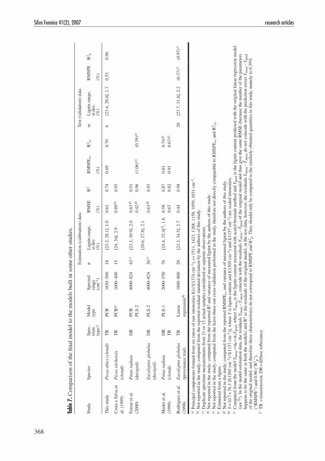
Comparable results from the models of the previous studies mentioned above are collated in Table 7. Differences in material naturally set limit to comparisons: none of the studies dealt with Norway spruce, and one of them was based on biodegraded material. In terms of RMSE, the fit of our model in the estimation data appeared fairly similar to those in the other studies; proportioned to the lignin content variation in the estimation data, however, the random error variation was seen to be of a larger magnitude in our model than in the other studies, which was reflected in the lower R2 value. (Note that 60 of our 272 candidate models had R2 larger than 0.95 in the estimation data, but their prediction performance in terms of especially RMSPE was judged far poorer than that of the final model). Only Meder et al. (1999) performed leave-one-out cross-vali-dation; they reported results rather similar to ours, although their models fitted slightly better to their estimation data. Rodrigues et al. (1998) were the only ones to use independent test data: although superior in the fit, their model appeared to equal our model in the prediction performance. Only Costa e Silva et al. (1999) applied their model to the independent prediction data of 83 samples with no lignin content measurements; they reported remarkably uniform standard errors of prediction between 0.86–0.97% (mean 0.89%, standard deviation 0.030 %), the uniformity prob-ably stemming partly from the replicate nature of the data and partly from the small number of intensity variables (6) involved in the model; on average, our model predicted with similar mag-

nitude of estimated uncertainty (Table 4), but the variation on standard errors of prediction was far larger, apparently due to the far larger amount of spectral information incorporated in the model.

The model estimation and test data sets of this study were rather small, although not out of line with most of the other similar studies (Table 7). This naturally limits the range of usage of this kind of empirical model, which is not, however, a serious defect from our point of view: we did not pursue large variation in lignin content or in other chemical properties of the samples, because we only wanted to build a model for prediction in a limited kind of clonal data, that is, the model was intended to be applied only to samples that can be regarded very similar to those in the estimation data. The empirical modelling procedure pre-sented here is, however, applicable to all kind of wood material, and a similar model could easily be built for e.g. natural or biodegraded samples.

4.2 Variation in Lignin Content

In this study Norway spruce trees from Loppi showed a higher sapwood lignin content than trees from Imatra or Kangasniemi. This may be due to the higher growth rate in Loppi (Raiskila et al. 2006b). The clone B the sapwood lignin content of which was the lowest had the slowest growth rate. The lignin content (23.17–27.79%) is slightly less than reported values for Norway spruce (27.5–28.9%) (Brolin et al. 1995, Anttonen et al. 2002). The lignin content has been found to be affected by the growth rate of trees e.g. in a fertilisation test (Anttonen et al. 2002). The lignin content is influenced by the growth rate possibly because of the changes in the relative amounts of cellulose rich secondary layers of cell wall and highly lignified middle lamella and by the relative amounts of earlywood and cellulose rich latewood (Anttonen et al. 2002). The purpose of cloning in the 1970’s was to increase the growth rate of trees. The three cutting clones (A, B, C) chosen for study were genetically uniform mate-rial and have grown in the different environments. The growth sites Loppi and Imatra were nutrient rich old agricultural lands and Kangasniemi was a medium fertile Myrtillus-type forest (Cajander 1926). The growth rate and wood properties of the

368


Tabl

e 7.

Com

pari

son

of th

e fin

al m

odel

to th

e m

odel

s bu

ilt in

som

e ot

her

stud

ies.

Est

imat

ion

(cal

ibra

tion)

dat

aTe

st (

valid

atio

n) d

ata

Stud

ySp

ecie

sSp

ec-

trum

ty

pe j)

Mod

el

type

Spec

tral

ra

nge

(cm

–1)

nL

igni

n ra

nge,

st

.dev

. (%

)

RM

SE

(%)

R2

RM

SPE

cv

(%)

R2 cv

mL

igni

n ra

nge,

st

.dev

. (%

)

RM

SPE

(%)

R2 p

Thi

s st

udy

Pic

ea a

bies

(cl

onal

)T

RPC

R18

50–5

0018

[23.

2, 2

8.1]

, 1.0

0.61

0.74

0.69

0.70

6[2

3.4,

28.

0], 1

.70.

530.

90

Cos

ta e

Silv

a et

al

. (19

99)

Pic

ea s

itch

ensi

s (c

lona

l)T

RPC

Ra)

1600

–400

15[2

4, 3

4], 2

.90.

89 b)

0.93

Ferr

az e

t al.

(200

0)P

inus

rad

iata

(d

ecay

ed)

Euc

alyp

tus

glob

ulus

(d

ecay

ed)

DR

DR

PCR

PLS-

2

PLS-

2

4000

–824

4000

–824

42 c)

26 c)

[23.

3, 3

0.9]

, 2.0

[20.

6, 2

7.8]

, 2.1

0.63

d)

0.42

d)

0.63

d)

0.91

0.96

0.93

(1.0

6) e)

(0.3

9) e)

Med

er e

t al.

(199

9)P

inus

rad

iata

(c

lona

l)D

RT

RPL

S-1

2000

–550

76[2

4.4,

32.

4] f)

, 1.6

0.58

0.67

0.87

0.82

0.81

0.91

0.74

g)

0.67

g)

Rod

rigu

es e

t al.

(199

8)E

ucal

yptu

s gl

obul

us

(pro

vena

nce

tria

l)T

RL

inea

r re

gres

sion

h)18

00–8

0020

[23.

3, 3

4.5]

, 2.7

0.44

0.98

20[2

3.7,

31.

8], 2

.2(0

.37)

i)(0

.97)

i)

a) Pr

inci

pal c

ompo

nent

s fo

rmed

fro

m s

ix r

atio

s of

raw

inte

nsiti

es I

(i) /

I(13

74 c

m–1

), i

= 1

511,

142

3, 1

268,

115

8, 1

059,

103

1 cm

–1.

b) N

ot r

epor

ted

in th

e st

udy;

com

pute

d fr

om th

e re

port

ed r

esid

ual s

tand

ard

devi

atio

n by

the

auth

ors

of th

is s

tudy

.c)

D

uplic

ate

spec

trum

mea

sure

men

ts f

rom

21

or 1

3 ac

tual

sam

ples

con

side

red

as s

epar

ete

obse

rvat

ions

.d)

Not

rep

orte

d in

the

stud

y; c

ompu

ted

from

the

repo

rted

R2

and

vari

ance

of

mea

sure

d lig

nin

by th

e au

thor

s of

this

stu

dy.

e) N

ot r

epor

ted

in th

e st

udy;

com

pute

d fr

om th

e le

ave-

thre

e-ou

t cro

ss-v

alid

atio

n pe

rfor

med

in th

e st

udy,

ther

efor

e no

t dir

ectly

com

para

ble

to R

MSP

Ecv

and

R2 cv

.f)

E

stim

ated

fro

m a

figu

re.

g) N

ot r

epor

ted

in th

e st

udy;

com

pute

d fr

om th

e re

port

ed R

MSP

Ecv

and

var

ianc

e of

mea

sure

d lig

nin

by th

e au

thor

s of

this

stu

dy.

h) Y

= 1

0.7

+ 7

6.3

[I(1

505

cm–1

) / I(

1157

cm

–1)]

, whe

re Y

is li

gnin

con

tent

and

I(1

505

cm–1

) an

d I(

1157

cm

–1)

are

scal

ed in

tens

ities

.i)

C

ompu

ted

from

the

mod

el Y

mea

s = a

0 + a

1Ypr

ed, w

here

Ym

eas i

s th

e lig

nin

cont

ent m

easu

red

with

ace

tyl b

rom

ide

met

hod

and

Ypr

ed is

the

ligni

n co

nten

t pre

dict

ed w

ith th

e or

igin

al li

near

reg

ress

ion

mod

el

(see

h)).

In

the

mod

el e

stim

atio

n da

ta, t

he r

esid

uals

Ym

eas –

Ym

eas c

oinc

ide

with

the

resi

dual

s Y

mea

s – Y

pred

of

the

orig

inal

mod

el a

nd th

us g

ive

the

sam

e R

MSE

(be

caus

e th

e nu

mbe

r of

the

para

met

ers

happ

ens

to b

e th

e sa

me

in b

oth

the

mod

els)

and

R2

as th

e re

sidu

als

of th

e or

igin

al m

odel

; in

the

test

dat

a, h

owev

er, t

he r

esid

uals

Ym

eas –

Ym

eas d

o no

t coi

ncid

e w

ith th

e pr

edic

tion

erro

rs Y

mea

s – Y

pred

of

the

orig

inal

mod

el, a

nd th

eref

ore

thes

e ch

arac

teri

stic

s do

not

cor

resp

ond

to R

MSP

E a

nd R

2 p. T

hey

shou

ld o

nly

be c

ompa

red

to th

e si

mila

rly

obta

ined

qua

ntiti

es in

this

stu

dy, n

amel

y to

0.3

9%

(“R

MSP

E”)

and

0.9

6 (“

R2 p”

).j)

T

R =

tran

smis

sion

, DR

= d

iffu

se r

eflec

tanc

e.

369


clones are described in Raiskila et al. 2006b. In this study the effects of site, clone and site-

clone interaction on the amount of sapwood lignin were significant but not on the amount of heart-wood lignin. The variation in the heartwood and sapwood lignin between individual stems was high. Several biotic and abiotic factors affect the growth of trees and thus, even the trees belong-ing to the same clone showed a large variation in lignin content. The mean lignin content of heartwood (26.23%) was slightly higher than that of sapwood (25.42%) and our results are in accordance with earlier results. The lignin con-tent has been reported to decrease significantly in the radial direction from heartwood (28.3%) to sapwood (27.7%) and to be the lowest in the transition zone (27.3%) (Bertaud and Holmbom 2004). In earlier studies with 1-year-old plants and 9-year-old trees the lignin content did not vary significantly within and between full-sib families but was higher in trees than in plants and a standard error for the trees was lower than for the plants (Wadenbäck et al. 2004). The amount of lignin is also affected by the reaction wood formation (Barnett and Jeronimidis 2003) and the ‘pseudo lignification’ during heartwood forma-tion (Magel 2000).

The annual variation in the amount of early-wood lignin was significant. The lignin content (24.64–28.77%) is slightly higher than reported values for earlywood (23–24%) (Gindl and Grab-ner 2000). In the earlier studies with Norway spruce the earlywood lignin content (32.2%) has been found to be significantly higher than the latewood lignin content (29.8%) but no clear dif-ferences between the annual rings were observed, however they studied only one stem (Bertaud and Holmbom 2004). One reason for the high variation between rings could be the selection of annual rings with very high and low weight density and variable ring width. However the earlywood lignin content did not correlate with the earlywood density. Also the annual variation in the growth and the weight density has been found to be significant and the growth increments did not correlate linearly with the weight density in this rapidly-growing clone material (Raiskila et al. 2006b).

5 ConclusionsA PCR-based method for predicting the relative amount of total lignin in clonal Norway spruce wood from FTIR transmission spectra was devel-oped. Using some modelling practices (all-subset regression; model selection based on combination of RMSE and RMSPECV in the estimation data and RMSPE in the test data) that, despite being standard in statistics, have not been frequently applied in FTIR or NIR modelling studies, a model with no over-fitting in the estimation data and good prediction performance in the test data was obtained. For a set of samples representing the same three clones growing in the same three sites as the samples in the modelling data, the model was seen to produce realistic lignin content predictions with satisfactory estimated precision.

By the analysis of the model estimation and test data pooled with the prediction data, site, clone and site-clone interaction were found to have a significant effect on sapwood lignin content. The model was also used to predict the lignin content in the earlywood of 45 individual annual rings; by the analysis of these predictions, the annual variation in the amount of earlywood lignin was significant and the variation between individual stems was large.

The method requires only a simple sample prepara-tion, and once the spectra have been recorded, it is fast and simple to use. A similar model, easily built by following the presented modelling procedure, could prove very advantageous when the natural genetic variation in lignin contents or variation caused by growth rate is determined e.g. in the extensive native stands of Norway spruce.

Acknowledgements

The Academy of Finland is gratefully acknowl-edged for the financial support of a programme on Sustainable Use of Forest Resources (Grant no: 52773). The authors thank Ph.D. Matti Sarén for his help with Matlab macro construction and Ph.D. Riikka Piispanen for her help with the sta-tistical analysis. We thank Ms. Irmeli Luovula, Mr. Tapio Nevalainen and Mr. Tapio Järvinen for skilful technical help.

370


ReferencesAnttonen, S., Manninen, A.-M., Saranpää, P., Kainulai-

nen, P., Linder, S. & Vapaavuori, E. 2002. Effects of long-term nutrient optimisation on stem wood chemistry in Picea abies. Trees 16: 386–394.

Barnett, J.R. & Jeronimidis, G. 2003. Reaction wood. In: Barnett, J.R & Jeronimidis, G. (eds.). Wood quality and its biological basis. Blackwell Publish-ing Ltd., Oxford. p. 118–136.

Belsley, D.A., Kuh, E. & Welsch, R.E. 1980. Regres-sion diagnostics: identifying influential data and sources of collinearity, John Wiley & Sons, New York. 292 p.

Bertaud, F. & Holmbom, B. 2004. Chemical composi-tion of earlywood and latewood in Norway spruce heartwood, sapwood and transition zone wood. Wood Science and Technology 38: 245–256.

Brolin, A., Norén, A. & Ståhl, E.G. 1995. Wood and pulp characteristics of juvenile Norway spruce: a comparison between a forest and an agricultural stand. Tappi J 78(2): 203–214.

Cajander, A.K. 1926. The theory of forest types. Acta Forestalia Fennica 29(3). 108 p.

Costa e Silva, J., Nielsen, B.H., Rodrigues, J., Pereira, H. & Wellendorf, H. 1999. Rapid determination of the lignin content in Sitka spruce (Picea sitchensis (Bong.) Carr.) wood by Fourier transform infrared spectrometry. Holzforschung 53: 597–602.

Dence, C.W. 1992. The determination of lignin. In: Lin, S.Y. & Dence, C.W. (eds.). Methods in lignin che-mistry. Springer-Verlag, Heidelberg. p. 33–61.

Faix, O. 1992 Fourier transform infrared spectroscopy. In: Lin, S.Y. & Dence, C.W. (eds.). Methods in lignin chemistry. Springer-Verlag, Heidelberg, p. 83–109.

— & Böttcher, J.H. 1992. The influence of particle size and concentration in transmission and diffuse reflectance spectroscopy of wood. Holz als Roh- und Werkstoff 50: 221–226.

Ferraz, A., Baeza, J., Rodriguez, J. & Freer, J. 2000. Estimating the chemical composition of biode-graded pine and eucalyptus wood by DRIFT spec-troscopy and multivariate analysis. Bioresource Technology 74: 201–212.

Fukushima, R.S. & Hatfield, R.D. 2001. Extraction and isolation of lignin for utilization as a standard to determine lignin concentration using the acetyl bromide spectrophotometric method. Journal of Agricultural and Food Chemistry 49: 3133–3139.

Gierlinger, N., Schwanninger, M., Hinterstoisser, B. & Wimmer, R. 2002. Rapid determination of heart-wood extractives in Larix sp. by means of Fourier transform near infrared spectroscopy. Journal of Near Infrared Spectroscopy 10: 203–214.

Gindl, W. & Grabner, M. 2000. Characteristics of spruce [Picea abies (L.) Karst.] latewood formed under abnormally low temperatures. Holzforschung 54: 9–11.

Hatfield, R. & Fukushima, R.S. 2005. Can lignin be accurately measured? Crop Science 45: 832–839.

— , Grabber, J., Ralph, J. & Brei, K. 1999. Using the acetyl bromide assay to determine lignin concentra-tions in herbaceous plants: some cautionary notes. Journal of Agricultural and Food Chemistry 47: 628–632.

Hergert, H.L. 1971. Infrared spectra. In: Sarkanen, K.V. & Ludwig, C.H. (eds.). Lignins; occurrence, forma-tion, structure and reactions. Wiley-Interscience, New York. p. 267–297.

Iiyama, K. & Wallis, A.F.A. 1988. An improved acetyl bromide procedure for determining lignin in woods and wood pulps. Wood Science and Technology 22: 271–280.

Jolliffe, I.T. 2002. Principal component analysis. 2nd ed. Springer-Verlag, New York. 487 p.

KCL. 1982. Massan ja puun kokonaisligniinipitoisuus [Total lignin content of wood and pulp]. KCL, Espoo, Finland, 115b. 3 p. (In Finnish).

Magel, E.A. 2000. Biochemistry and physiology of heartwood formation. In: Savidge R.A., Barnett, J.R. & Napier, R. (eds.). Cell and molecular biology of wood formation. BIOS Scientific Publishers Ltd, Oxford. p. 363–376.

Mardia, K.V., Kent, J.T. & Bibby, J.M. 1979. Multivari-ate analysis. Academic Press, London. 521 p.

Martens, H. & Næs, T. 1989. Multivariate calibration. John Wiley & Sons, Chichester. 419 p.

Meder, R., Gallagher, S., Mackie, K.L., Böhler, H. & Meglen, R.R. 1999. Rapid determination of the chemical composition and density of Pinus radiata by PLS modelling of transmission and dif-fuse reflectance FTIR spectra. Holzforschung 53: 261–266.

Næs, T., Isaksson, T., Fearn, T. & Davies, T. 2002. A user-friendly guide to multivariate calibration and classification. NIR publications, Chichester. 344 p.

Panshin, A.J. & de Zeeuw, C. 1980. Textbook of wood technology. Structure, identification, properties,

371


and uses of the commercial woods of the United States and Canada. 4th ed. McGraw-Hill, New York. 722 p.

Raiskila, S., Fagerstedt, K., Laakso, T., Saranpää, P., Löija, M., Paajanen, L., Mahlberg, R. & Ritschkoff, A.-C. 2006a. Polymerisation of added coniferyl alcohol by inherent xylem peroxidases and its effect on fungal decay resistance of Norway spruce. Wood Science and Technology 40(8): 697–707.

— , Saranpää, P., Fagerstedt, K., Laakso, T., Löija, M., Mahlberg, R., Paajanen, L. & Ritschkoff, A.-C. 2006b. Growth rate and wood properties of Norway spruce cutting clones on different sites. Silva Fen-nica 40(2): 247–256.

Rodrigues, J., Faix, O. & Pereira, H. 1998. Determi-nation of lignin content of Eucalyptus globulus wood using FTIR spectroscopy. Holzforschung 52: 46–50.

Saranpää, P. 2002. Ensiharvennuskuusen raaka-aineominaisuudet. In: Saranpää, P. & Verkasalo, E. (eds.). Kuusen laatu ja arvo. Finnish Forest Research Institute, Research Papers 822. p. 61–70. (In Finnish).

Sjöström, E. 1993. Wood chemistry – fundamentals and applications. Academic Press, Inc., USA. 293 p.

Venables, W.N. & Ripley, B.D. 1997. Modern applied statistics with S-PLUS. 2nd ed. Springer-Verlag, New York. 548 p.

Wadenbäck, J., Clapham, D., Gellerstedt, G. & von Arnold, S. 2004. Variation in content and compo-sition of lignin in young wood of Norway spruce. Holzforschung 58: 107–115.

Walker, J.C.F. 1993. Primary wood processing, prin-ciples and practice. Chapman & Hall, London. 595 p.

Weisberg, S. 1985. Applied linear regression. John Wiley & Sons, New York. 324 p.

Westad, F. & Martens, H. 2000. Variable selection in near infrared spectroscopy based on significance testing in partial least squares regression. Journal of Near Infrared Spectroscopy 8(2): 117–124.

Total of 36 references

ftir spectroscopic prediction of klason and acid soluble ... · with the klason lignin (gravimetric...

Documents