SOLAR ASTRONOMY: THE LITTLE ICE AGE

W

published in A&G, Astronomy and Geophysics, April 2017

Lockwood, M., M.J. Owens, E. Hawkins, G.S. Jones and I.G. Usoskin (2017) Frost fairs, sunspots and the Little Ice Age ,

Astron. & Geophys., 58 (2), 2.17-2.23, doi: 10.1093/astrogeo/atx057

Frost fairs, sunspots and the Little Ice Age Mike Lockwood, Mat Owens, Ed Hawkins, Gareth S. Jones and Ilya Usoskin examine the links

between the solar Maunder minimum,

the Little Ice Age and the freezing of

the River Thames.

here spin doctors, politicians and newspaper editors understand well that a name alters how

something is perceived, scientists know that a name does not change the reality one iota. By virtue of the name awarded to it, the “Little Ice Age” has been associated with full ice ages. The name Little Ice Age has also become almost synonymous with the Maunder minimum

in solar activity in the minds of many people. Hence it has even become possible to build semantic arguments that imply there is some sort of link between solar activity and ice ages – and evidence for major control of climate by solar activity is often offered in the form of the occurrence of frost fairs on the Thames in London. This paper discusses the true relationships, or lack of them, between these different events.

Ice Ages

Before discussing the “Little Ice Age” we should be clear what a proper ice age is. Global temperatures can be inferred from polar ice cores using the isotopic composition of the water molecules. In particular, the amounts of deuterium (

2H)

and of the 18

O isotope present in the ice

are lower if temperatures at lower latitudes at the time of their deposition were depressed. This is because it takes more energy to evaporate the water molecules containing these heavier isotopes from the surface of the ocean and, in addition, as the moist air containing the evaporated water is transported polewards and cools, the water molecules containing the heavier isotopes are more easily lost by precipitation. Both processes mean that less deuterium and

18O reaches the polar

regions if global temperatures are lower. This “fractionation” effect can be calibrated and so a record of temperatures back to the distant past can be generated from measurements of the abundance of 2H and/or

18O in deep cores into ancient

polar ice sheets. Figure 2 shows

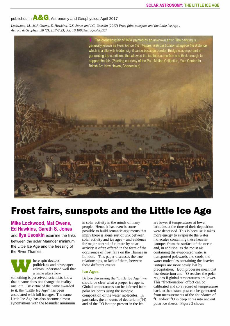
1. The great frost fair of 1684 painted by an unknown artist. The painting is

generally known as Frost fair on the Thames, with old London Bridge in the distance

which is a title with hidden significance because London Bridge was important in

generating the conditions that allowed the ice to become firm and thick enough to

support the fair. (Painting courtesy of the Paul Mellon Collection, Yale Center for

British Art, New Haven, Connecticut).

SOLAR ASTRONOMY: THE LITTLE ICE AGE

temperatures deduced from ice cores taken at the Vostok station in Antarctica that are deep enough to allow us to see the variation over the past 420,000 years (from Petit et al., 1999). The temperature is shown as the difference relative to present day values (in other words as a temperature “anomaly”, T ). The ice cores reveal that global temperature is characterised by rapid rises, followed by gradual declines. These cycles are known to be driven by the Milankovitch cycles in Earth’s orbital characteristics but are still not fully understood.

The feature to note here is the extremely large difference between the relatively short, warm “interglacials” (T around or exceeding zero, coloured red) and the cold “glaciations” (usually known as “ice ages” and here coloured blue), in which average temperatures are lower than during the present interglacial, (the “Holocene”) by up to 8C. The effects of such low global temperatures in the ice ages are very profound, with polar ice sheets expanding to cover temperate latitudes and fundamental changes to the patterns of precipitation and temperature. During the last glacial maximum, ice sheets spread down to cover Scotland, Wales and northern England (Bowen et al., 2002) and insect studies reveal temp-eratures in southern England averaged about 8C with minimum and maximum seasonal values of 30C and +8C (Atkinson et al., 1987). Under such conditions the UK, like most of northern Europe (to which the UK was joined by the Doggerland land bridge), was abandoned by humans and the archaeological record shows that it was permanently recolonised only after the ice age started to come to an end (Barton et al., 2003).

The Little Ice Age

Compared to the changes in the proper ice ages, the so-called “little ice age” (LIA) is a very short-lived and very puny climate and social perturbation. The term was introduced into the scientific literature by François E. Matthes in 1939 in relation to glacier advances in the Sierra Nevada, California. However it is somewhat misleading and is open to misuse as it implies much greater similarities to a full ice age than really exist: hence some climate scientists argue the name should be abandoned (see discussion by Matthews and Briffa, 2005).

The black line in figure 3(b) shows the best estimate of the variation in the average air surface temperature in the

northern hemisphere since 850 AD. This is a combination by Masson-Delmotte et al. (2013) of 18 separate reconstructions and was presented in the 5

th assessment

report (AR5) of the International Panel on Climate Change (IPCC). Each of these reconstructions employs multiple temperature proxies, including data from boreholes, corals and sclerosponges, ice cores, insect numbers, instrumental data, pollens, lake levels, loess (wind-blown silt), glacier extents, plant macrofossils, diatoms, molluscs, foraminifera, dinoflagellates, ostracods, heavy minerals, grain-size, trace elements in speleothems, dendrochronology and historical records (recorded freeze/thaw dates, harvest yields and dates, etc.) (see review of techniques by Jones and Mann, 2004). The colours give the probability density function (pdf) in each year, that allow for both the computed uncertainties in each reconstruction and the differences between the reconstructions. The larger the peak pdf, the narrower is the distribution and so the closer the agreement between the various reconstructions. Temperatures in figure 3 are presented as the anomaly with respect to the average for 1961-1990, TNH. It should be recognised that figure 3(b) represents a truly outstanding scientific achievement; it is arrived at though a huge variety of paleoclimate techniques and a colossal number of measurements from all over the northern hemisphere.

The LIA can be seen in figure 3 as the dip in temperatures reaching minimum values around 1700. The first thing to note is that

the best estimate of the amplitude of the dip is, at most, 0.5C: this should be compared to the decreases in ice ages of about 8C shown in figure (2). Note also that the LIA persists for 500 years at most, compared to the 20,000 years of the last ice age. Several causes of the LIA have been proposed, including lows in solar radiation, heightened volcanic activity, changes in the ocean circulation, the inherent internal variability in global climate and increased human populations at high latitudes through the deforestation they brought about. The start and end dates of the LIA depend strongly on the temperature proxy used to derive them and on geographic region. Evidence from mountain glaciers suggest increased glaciation in a number of widely-spread regions around the 12

th century AD: these

include Alaska, New Zealand, America and Patagonia. However, the timing of maximum glacial advances in these regions differs considerably, suggesting that they may represent largely independent regional climate changes, not a globally-synchronous increased glaciation. Individual studies agree with the view of the LIA given in figure 3(b): for example, based on about 150 samples of plant material collected from beneath ice caps on Baffin Island and in Iceland, Miller et al. (2012) find that cold summers and ice growth began abruptly between 1275 and 1300, followed by "a substantial intensification" from 1430 to 1455. Figure 3(c) shows the volcanic

2. The variation of global temperatures over the past 0.42 million years deduced from

ice cores taken at Vostok station, Antarctica (from Petit et al., 1999).

SOLAR ASTRONOMY: THE LITTLE ICE AGE

aerosol optical depth (AOD) inferred from sulphate abundances found in Greenland and Antarctic ice cores (Crowley and Unterman, 2013). The largest spike is associated with the major volcanic eruption in 1257 of the Samalas volcano, next to Mount Rinjani on the island of Lombok, Indonesia. This as one of the largest eruptions during the Holocene and figure 3 shows it probably caused a temporary drop in TNH, but perhaps not as great as the sulphate yield suggests it should. (For example, the eruption of Tambora in 1815, seen in figure 3(c) as a smaller spike in AOD, is associated with a drop in TNH of similar magnitude). The Samalas eruption has been postulated as the driver of glacial advances and the growth in the Atlantic ice pack that mark the start of the LIA, as

defined from the cryosphere. The intensification noted by Miller et al. (2012) after 1430 is associated with a steep drop in TNH which has been linked to a burst of volcanic activity (reflected in the AOD). This can also be considered as the start date of the LIA, as defined from TNH. The lowest temperatures in the LIA, between about 1570 and 1730, are during a period of almost continuous, but smaller, volcanic activity.

The problem with the name Little Ice Age is that it implies a period of unremitting cold when even summer temperatures barely get above zero, as was seen at middle latitudes during the ice ages proper. This idea is frequently bolstered using paintings from the time, such as Pieter Bruegel the Elder’s Hunters in the

Snow, painted in 1565 (see figure 4). What is rarely mentioned in this context is that this painting is thought to be one of a series of 12 that Bruegel produced that year, one for each month (Hunters in the Snow being for January) and that none of the 4 others that survive show a landscape in the grip of deep cold: indeed both Haymaking (July) and The Harvesters (August, also shown in figure 4) depict warm summer days with workers gathering a plentiful harvest. Even The Return of the Herd (thought to be the painting for November) and The Gloomy Day (known to be for February) show a landscape free of snow. The Twelve Months paintings depict a Europe that is very far from the uninhabitable state of an ice age. Hunters in the Snow was clearly influenced by the scenery Bruegel saw when crossing the Alps on a trip to Italy in 1551/2, but he also painted other snow-bound scenes of the low countries in 1565 (and even the later wintry paintings by his son, Pieter Brueghel the Younger, were based on sketches that his father had made in 1565). We also know that it was in the December of that winter that the Thames in London froze sufficiently for Elizabeth I to walk on it, suggesting it may have been an unusually harsh winter throughout Europe. Combining all the available chronicles there are 6 reported severe winters in England in the 50 years prior to 1565 and 6 in the 50 years after. This is a much higher occurrence rate than we experience today, but it is not an ice age, little or otherwise. Many aspects of the paintings of Bruegel-the-Elder make them brilliant and innovative artworks rather than records of climate: they were revolutionary in depicting winter at all, it previously having been seen as a dull, dreary, even frightening, season and avoided by artists. Hence it is possible that his winter scenes are primarily testament to his artistic inventiveness and boldness and it is even possible that he painted them, not because they were typical but because they were unusual.

The Maunder Minimum

The husband and wife astronomers, Walter and Annie Maunder studied the occurrence of sunspots. In 1890, Walter presented a paper on the work of Gustav Spörer to the Royal Astronomical Society and in 1894 published a paper entitled "A prolonged sunspot minimum". The interval when the Sun was almost free of sunspots (c.1645-1715) had been noted by Spörer and the Maunders’ work to

3. The Variations around the “Little Ice Age”. (a) Sunspot number estimates: (mauve line) 11-

year running means the extended sunspot number sequence of Lockwood et al. (2014), <RC>;

(green line) smoothed sunspot numbers derived from dendrochronology data (14C abundance

measurements), R14C (Usoskin et al., 2014). The grey area gives the computed uncertainty in

R14C. (b) A combination of 18 paleoclimate reconstructions of the Northern hemisphere mean air

surface temperature anomaly TNH by Masson-Delmotte (2013). The colour contours give the

probability distribution function (pdf) obtained by combining the 18 different reconstructions and

allowing for the uncertainty in each. The peaks (mode values) of the annual pdfs are joined by

the black line. The blue dots show 10-year running means of TNH from the HadCRUT4

observational record (Morice et al., 2012). For both datasets, the anomaly is computed relative

to a reference interval of 1961-1990. (c) The volcanic aerosol optical depth (AOD) at 550 nm

derived from sulphate abundances measured in Greenland and Antarctic ice sheet cores (from

Crowley and Unterman, 2013).

SOLAR ASTRONOMY: THE LITTLE ICE AGE

confirm its existence resulted in it now being termed the “Maunder minimum”. A prior period of minimal solar activity (c.1420-1550), identified from

14C

abundances in tree rings, is now named after Spörer. The top panel of figure 3 shows the sunspot number (decadal means of observations and inferred from 14

C) and demonstrates both the Spörer and Maunder minima.

There is no straightforward connection in figure 3 between the sunspot variations and the variations in TNH. One can identify times when the two appear to vary together but for some of these TNH follows sunspot number R but for others it is the other way round. Of particular note are the most recent data, in which the opposite sense of trend in TNH and R that Lockwood and Fröhlich (2007) noted as beginning in 1985, has continued to the present day. It is, however noticeable that the lowest TNH of the LIA did occur during the MM. For this reason, it has become increasingly common to associate the LIA with the MM, indeed in some instances the two terms have even been used interchangeably.

Frost Fairs on the Thames in London

The frost fairs held on the frozen river Thames in London are often invoked as evidence for an effect of the MM on climate. Such evidence is “anecdotal” in

nature and, as pointed out by Jones and Mann (2004) and Jones (2008), can be misleading for a host of different reasons. The first such fair is often said to be in 1608, and indeed this appears to be the first time that the name “frost fair” was used. However, there is a dependence on the definition of what constitutes a “frost fair” to consider. Eyewitness reports from as early as 250 AD talk of social gatherings on the river which in that year was frozen solid for six weeks. (Note that there is always the potential for confusion between “old” (Julian) and “new” (Gregorian) dates in these reports as the correction can be omitted, applied in error or even applied multiple times). The chronicler Thomas Tegg reports that the Thames froze for over six weeks in 695 and that booths to sell goods were erected on it (Tegg, 1835). Fires were lit and sports organised on the frozen river in 1309. It is probable that frost fairs became fashionable through the influence of Flemish immigrants from the Low Countries, where such events had been common for some time, and how much this contributed to their increased occurrence, as opposed to an increased occurrence in the required meteorological conditions, is not known. Another problem with attaching significance to the frost fair dates is that it is certainly not true that a frost fair was held during every winter in which the river was sufficiently frozen. In the winter of 923, the river

carried loaded horse carts for 13 weeks and in both 1150 and 1410 the same was true for 14 weeks, but no frost fair is mentioned in the records. There are potential social, political, economic, health and, possibly, supply shortage reasons for this. Frost fairs were often bawdy and unruly events and so were sometimes discouraged by puritanical authorities. It is noticeable that between the frost fairs of 1763 and 1789 there were 5 winters in which the Thames was reported as freezing yet there is no known record of a frost fair being held. The winter of 1776 was particularly cold with heavy snow and the river was known to be frozen. However, that winter London was also hit by an influenza epidemic, one that is estimated to have killed 40,000 people in England. The year 1740 may point to other problems. The Thames was frozen solid for about eight weeks, but before then ice floes, fog and damage to riverside wharfs disrupted shipping and there were great shortages of fuel, food and drink supplies in the city. Attempts to unload cargoes upstream and bring them by road were hampered by heavy snow. Andrews (1887) quotes a source as saying “the watermen and fishermen … and the carpenters, bricklayers … walked through the streets in large bodies, imploring relief for their own and families' necessities; and, to the honour of the British character, this was liberally bestowed. Subscriptions were also made

(a) (b)

4. Two paintings by the Dutch painter Pieter Bruegel the Elder (c.1525 –1569) that are part of the series known as the Twelve Months,

commissioned by a wealthy patron in Antwerp, Niclaes Jonghelinck and painted in 1565, during the Little Ice Age. On the left is the January

painting, Hunters in the Snow (also known as The Return of the Hunters) which is often used to re-inforce the idea of unremittingly cold conditions

in the Little Ice Age. Almost never shown in that context is the painting for August, the Harvesters (on the right) which depicts workers gathering

crops on a warm summer’s day. The other surviving pictures in the series are The Gloomy Day (February), Haymaking (July), and The Return of

the Herd (probably November) – none of which give any indication of unusually cold conditions. If Bruegel did paint all 12 months then, sadly, 7

have been lost. (Paintings courtesy of Kunsthistorisches Museum in Vienna and the Metropolitan Museum of Art, New York)

SOLAR ASTRONOMY: THE LITTLE ICE AGE

in the different parishes, and great benefactions bestowed by the opulent, through which the calamities of the season were much mitigated”. (This is true to an extent, for example Sir Robert

Walpole, the philanthropist and, effectively Britain’s first prime minister, donated £1000 – almost £0.1m at today’s prices). In 1740 a frost fair was held despite the crisis, but in other years such

circumstances may have made it impossible. Records indicate that harsh winters on their own did not generate food shortages in London, but harsh winters at times of economic depression did and how devastating they were for the population depended greatly on the readiness of welfare provision (Post, 1985). Incidentally, in 1740 temperatures were exceptionally low on some days: the Reverend Derham in nearby Upminster, Essex (a regular and careful observer of meteorological and auroral phenomena and Fellow of the Royal Society), recorded the frost of this winter as the most severe on record and that the temperature on 3rd January fell to 24C. This was after the end of the Maunder minimum - indeed Derham himself had noted the return of aurora over Upminster in 1707, 1726, and 1728 (Lockwood and Barnard, 2015). The monthly mean Central England Temperatures (see next section) were 2.8C in January and 1.6C February that year.

Because of these multiple reasons why the conditions favourable for frost fairs were not always exploited, we here look at the dates of both frost fairs and of reports that the Thames was frozen sufficiently for people to walk on it (and that the tidal variations did not break up the ice). However, this record is not homogeneous and the number of reports of such a freezing Thames increases with time over the years 1400-1600 as the number of surviving diaries and chronicles increases. It is notable that two of the three reports in 50 years of the mid-16

th century exist

because of royalty: in 1537 Henry VIII, with his then queen (Jane Seymour) rode in sleigh on the ice-bound river from Whitehall to Greenwich and at Christmas 1564 Queen Elizabeth I is said to have walked and, in some accounts practised archery, on the frozen Thames. That it took royal involvement to generate an account, may indicate an under-reporting of the phenomenon in other years at this time and many of the chronicles describe some deep and prolonged frosts in England during winters for which we have no reports of the Thames freezing .

There are several books published on the frost Fairs but perhaps the most interesting is that by Davies (1814). The title is entertainingly long and often shortened to “Frostiana”. An interesting aspect is that the author (and printer) claims that the first page was printed by a press installed on the river ice at the 1814 (and last) frost fair. In figure 5, the dates of known frost fairs are marked by

5. Sunspot number estimates: (grey area) the extended sunspot number sequence of

Lockwood et al. (2014), RC; (mauve line) 11-year running means of RC <RC>; (green line)

smoothed sunspot numbers derived from dendrochronology 14C abundance measurements,

R14C (Usoskin et al., 2014). (b) The mode of the distribution of the reconstructions of the

Northern hemisphere mean air surface temperature anomaly by Masson-Delmotte (2013)

extended to after 1997 using the HadCRUT4 observations record (Morice et al., 2012), TNH.

The black line is 0.7<Tann> where Tann is the annual mean of the Central England Temperature

(CET) and the averaging is done over 10 years. (c) The anomaly in the lowest monthly mean

CET in each winter, Tmin. The mean of Tmin over the reference period (1961-1990) is 2.6C and

so the horizontal line drawn at Tmin = 2.6C corresponds to Tmin = 0C. (d) The anomaly in

December, January, February means in CET, TDJF. The mean of TDJF over the reference period

(1961-1990) is 4.0C and so the horizontal line drawn at TDJF = 4.0C corresponds to TDJF =

0C. (e) The anomaly in June, July, August means in CET, TJJA. The mean of TJJA over the

reference period (1961-1990) is 15.3C. (f). The volcanic aerosol optical depth (AOD) at 550 nm

derived from sulphate abundances in ice sheet cores by Crowley and Unterman (2013). All

anomalies are with respect to the mean for the reference interval 1961-1990. Vertical mauve

lines are the dates of frost fairs, of orange lines are reports of the Thames frozen solid. The

vertical dashed lines are the demolition of the old London bridge in 1825 and the completion of

the embankments with the opening of the Victoria embankment in 1870.

SOLAR ASTRONOMY: THE LITTLE ICE AGE

6. A cyclist, David Joel, rides on the

frozen River Thames at Windsor in 1963.

vertical mauve lines, whereas the dates in which the Thames was known to be frozen solid, sufficient for people to walk on it (yet there is no known record of a frost fair), are shown by orange vertical lines. These have been identified by surveying original diaries and chronicles (e.g., Davis, 1814; Tegg, 1835; Lowe, 1870; Andrews, 1887) and the newspapers of the day and the list agrees well that compiled by others (e.g., Lamb, 1977).

Central England Temperature records

The Central England temperature (CET) data set is the world’s longest instrumental record of temperature (Manley, 1953; 1974; Parker et al., 1992). It starts in 1659, near the start of the Maunder minimum, and continues to the present day. The CET covers a spatial scale of order 300 km which makes it a ‘small regional’ climate indicator, and to some extent it will reflect changes on both regional European (∼3000 km) and hemispheric scales but, without the averaging over the larger areas, will show considerably greater inter-annual variability. The measurements were (and still are) made in a triangular region between London, Bristol and Lancaster and always in rural locations: this means the data sequence is not influenced by the “urban heat island” effect and the growth of cities. In winter, the North Atlantic Oscillation (NAO), and associated changes in thermal advection, contribute a large fraction of the observed variability of CET. The CET does show a marked long-term warming trend (Karoly and Stott, 2006). Monthly means of CET are available for January 1659 onwards but the daily record begins 1

st January 1772 in

continues to the present day. The uncertainty in monthly means from November 1722 onwards and for 1699 -1706 inclusive (the latter period being largely based on Derham’s observations made in Upminster) is estimated to be 0.1 °C. For the other years between 1659 to October 1722, the best error estimate for the monthly means is 0.5°C.

Parts (c) – (e) of figure 5 show various sequences taken from the monthly CET data sequence. All are presented as a temperature anomaly T with respect to their mean value for 1961-1990 with red shaded areas for positive anomalies and blue for negative. In (c), the anomaly in the lowest monthly mean in each winter is shown, Tmin. It can be seen that there is an excellent agreement between the winters of large negative Tmin values and the dates of frost fairs and solid river

freezing. This agreement exists from the start of the CET data until 1825. If there is uncertainty when the first Thames frost fair took place, there is none about when the last was: it being almost the last time that the Thames ice was thick and firm enough to support one. That was in 1814. This frost fair lasted just 5 days (1-5 February) the river having frozen solid on the last day of January. An elephant was led across the river at Blackfriars and various booths and printing presses established on the ice. However the fair ended badly with a sudden thaw and many booths were lost and at least two young men lost their lives (such tragedies were quite common at the end of frost fairs). This may explain why 6 years later, when the river froze solid for the last time in London, no frost fair was held. After 1825, the Tmin values often fell to levels that had given frost fairs in previous years, but there are no reports of the river freezing to the same degree as before (although a woodcut from February 1855 shows people walking on the ice in central London, it also shows that the ice was not a complete covering). The mean of Tmin over the reference period (1961-1990) is 2.6C and so the horizontal line drawn at Tmin = 2.6C in figure 5(c) corresponds to Tmin = 0C, the freezing point of pure, static water. Although the freezing point of the brackish tidal water at London would be lower than 0C, freezing conditions for a whole month would not be necessary to build up a great enough thickness of ice (of order 10 cm) sufficient to support groups of people. Hence Tmin below 2.6C in monthly means would probably have been sufficient to enough to freeze the Thames solid. The reason why freezing increasingly failed to happen, even though monthly Tmin values repeatedly fell

below 2.6C, is almost certainly that in 1825 (marked by the first vertical black dashed) the old London Bridge was demolished. This bridge had many small arches and elements of a weir, which slowed the flow, allowing ice to form and thicken. The river flow was further increased by the building of the embankments, a programme completed with the opening of the Victoria embankment in 1870 (the second vertical dashed line). Andrews (1887) notes of the very cold winter of 1881 “it was expected by many that a Frost Fair would once more be held on the Thames” but does not explain why there was none. In 1883 and 1896 ice floes formed on the river but it did not freeze solid. Hence the end of the frost fairs and London Thames freezing was caused by the riverine developments rather than climate change. Jones (2008) notes that the low Tmin of 1963 did cause the Thames to freeze upstream of London at Windsor, sufficient for football matches and other activities to be pursued on the ice: by this time the size, banks and flow rate of the river at Windsor were all similar to those prevailing in London 200 years earlier, although the river at Windsor is not tidal.

Part (d) of figure 5 shows the winter (December, January and February) mean CET anomalies, TDJF. Agreement with the occurrence of Thames freeze dates is good, but not as consistent as for Tmin. This is not surprising because the cold snap required to freeze the river would depress the temperature in one month and so reduce Tmin but the three-month average need not be so greatly depressed if temperatures before and after the cold snap were not as low. Note the great inter-annual variability in the CET winter temperatures: the coldest winter (lowest TDJF) in the series is 1684 (the year of the most famous frost fair shown in figure 1) yet the 5

th warmest winter in the whole

series to date is just 2 years later. Hence even at the peak of the LIA there were exceptionally mild winters in England. Part (e) looks at the summer CET anomalies (means for June, July and August) and shows the agreement of cold summers and Thames freeze dates is even poorer. Indeed, several of the frost-fair years had relatively hot summers (bear in mind the anomalies are with respect to the CET JJA mean for 1961-1990 which is TJJA = +15.3C. Thus the CET data, like Bruegel’s paintings dispel the impression that the LIA was a period of unremitting cold – this is not the case as the cold winters were often interspersed with very mild winters and/or with hot summers.

SOLAR ASTRONOMY: THE LITTLE ICE AGE

Figure 5(b) shows the anomaly (again with respect to 1961-1990) in the mode of the pdf of the northern temperature, TNH, from the paleoclimate reconstructions used in figure 3(b). Clearly the averaging over a whole hemisphere has smoothed out the inter-annual variability in the seasonal CET data. Note the smaller range of the scale for this panel. The black line shows the annual mean CET anomaly that has been passed through a 20-year running mean filter to smooth out this inter-annual variability. It has also been divided by 1.4 for comparison. It can be seen that the CET shows a similar, long-term trend to the reconstructed northern hemisphere temperature since 1900 (but one that is larger by a factor of 1.4). Before 1900, we do see considerably more variability in the CET trend, but this is not unexpected because CET is small-regional climate measure and not a hemispheric or global one.

Potential causes of Thames freezing events

Panels (a) and (f) of figure 5 give indicators of the solar and volcanic aerosol variations. Panel (f) shows the

volcanic aerosol optical depth, AOD (at 550nm). It is apparent that many of the dates of reported Thames freezing events are soon after volcanic eruptions, even if in some cases the associated rise in AOD is relatively minor. This not always true, for example, the major rise in AOD thought to be caused by eruption of Kuwae (or potentially Tofua) in 1452/3 is not followed by a known report of the Thames freezing, the same is true for the peak AOD associated with a number of erupting volcanoes in 1441/2 and that associated with the eruption of Huaynaputina in 1600. The putative Kuwae/Tofua eruption is one of those that has been linked with the second pulse of the LIA. Thames freeze winters that could be associated with significant AOD rises (to within the estimated 1 year uncertainty in the ice sheet core dating) are 1595, 1640, 1677, 1695, 1811 and 1814. The largest peak in the AOD in the period covered by figure 5 is the major eruption of Tambora in July 1815. The effect of this can be seen in TNH, and in all the CET anomalies - including for summer (TJJA), the negative values of which in 1816 mark the so-called “year

without summer”. Eye-witness accounts tell us that the Tambora eruption certainly occurred after the 1814 frost fair, which might be related to the major unknown eruption inferred from the ice core data to have taken place 2 or 3 years earlier at tropical latitudes and followed soon after by 4 known eruptions. Hence it is probable that volcanic eruptions contributed to generating conditions that led to the Thames freezing over, but the lack of a clear one-to-one relationship indicates that they are not the only factor involved.

The grey area in Figure 5(a) gives the annual mean sunspot number composite of Lockwood et al. (2014a), RC. It should be noted that there is discussion about the most accurate sunspot number reconstruction (e.g. Lockwood et al., 2016), but there are greater problems that have been identified with the only other reconstructions that reach back to before the Maunder minimum. However, the differences between the reconstructions are not important here: we simply require a sequence that identifies both the Maunder and Dalton minima (c.1650-1710 and 1790-1825, respectively). The mauve line shows 11-year running means of R C. The green line is the sunspot number derived from

14C abundances

measured in tree rings which are used to extend the sunspot data to before the first observations. In the period of overlap with the sunspot observations there is good agreement between R14C and <RC> (the mauve line), where the averaging of RC is done over the sunspot cycle length of 11 years. The

14C data define the

Spörer minimum (c.1420-1550). Lockwood et al. (2010) noted that the coldest years in the CET winter temperatures (lowest TDJF), were at low solar activity but that low solar activity did not always lead to such cold winters. The most likely explanation of this potential solar influence on the occurrence frequency of cold European winters is being confirmed by numerical modelling which extends up into the stratosphere and allows for upper-end estimates of the long-term variability of the UV solar flux with solar activity, via its action on the stratospheric temperature gradient in the winter hemisphere (Ineson et al., 2015; Maycock et al., 2015). Hence low solar activity may well also have played a role in generating cold winters in the UK.

Figure 7 analyses the occurrence of Thames freezing events with solar activity and the northern hemispheric air surface temperature reconstructions. Panel (b)

7. The (a). 10-year means of sunspot numbers derived from 14C abundances R14C. (b) The

occurrence frequency fFT of winters in which the Thames is reported to have frozen solid

(computed for intervals 20 years long and 10 year apart). (c) the pdf (grey scale) of combined

reconstructions of the northern hemisphere temperature anomaly, TNH, and the optimum

(mode) value of the distribution (yellow line). The horizontal green and blue dot-dash lines are

at 0.22C and 0.44C (TNH anomalies with respect to the means for 1961-1990). In all

three panels the vertical green lines mark the Little Ice Age defined by the mode anomaly

TNH below the 0.22C threshold (termed LIA1 which covers 1437-1922); the vertical blue

lines mark the Little Ice Age defined by the mode TNH below the 0.44C threshold (termed

LIA2 which covers 1570-1726); the vertical red lines mark the Maunder Minimum set by the

decadal means of R14C below 15 (labelled MM and covering 1650-1717).

SOLAR ASTRONOMY: THE LITTLE ICE AGE

shows fFT, the occurrence frequency of winters in which the Thames was reported to freeze solid (computed in 20-year intervals with start times that are 10 years apart, so intervals overlap by 50%). Part (a) shows the decadal means of the sunspot number calculated from

14C

abundance found in tree rings, R14C. It can be seen that fTF and R14C show no clear relationship. The horizontal green and blue dot-dash lines in the bottom panel mark TNH anomaly levels (with respect to the mean for 1961-1990) of 0.22C and 0.44C. The mode value of the reconstructed TNH falls below these thresholds during the years 1437-1922 (here termed LIA1 and delineated in figure 7 by the vertical green lines) and 1570-1726 (here termed LIA2 and shown between the two vertical blue lines. The vertical red lines mark the Maunder Minimum set by the decadal means of R14C being below 15 (labelled MM and covering 1650-1717).

It can be seen that there was a rise in fFT that coincides with the Little Ice Age

defined by the lower threshold of TNH

(LIA2). However, there is a bigger peak in fFT at 1780-1800 that is after the end of LIA2 (but still within LIA1) when average northern hemisphere temperatures have risen again. This peak is also after the MM ended and when mean sunspot numbers R14C and <RC> exceed 50.

We conclude that winters in which the Thames froze, although well correlated with the lowest temperatures in the local observational record, the CET, are not at all good indicators of the hemispheric or global mean temperatures. The often-quoted result that they were enhanced during the solar Maunder minimum is false, Thames freeze years being slightly more frequent before the Maunder minimum began and also considerably more common 65 years after it ended. The association of the solar Maunder minimum and the Little Ice Age is also not supported by proper inspection and ignores the role of other factors such as volcanoes that mean that although the

LIA covers both the Spörer and Maunder solar minima, it also persisted, indeed deepened, during the active solar period between these two minima. The latest science indicates that low solar activity could indeed act to increase the frequency of cold winters in Europe, but that it is a phenomenon that is restricted to winter and is just one of a complex mix of factors. It is vital to avoid semantic arguments based on the name “the little ice age”: ice ages proper are a lot more than a period in which the frequency of somewhat colder winters is somewhat elevated. Lastly, if we must use the name “little ice age” we should know it for what it really was and our best insight into that comes not from anecdotal reports influenced by a great many factors, nor from speculating about the inspiration for a few artists 450 years ago, but from the truly colossal number of objective datapoints, derived by many scientists using a huge variety of sources and techniques, that have gone into the construction of figure 3(b).

AUTHORS Mike Lockwood, Mat Owens, Ed Hawkins (University of Reading, Reading), Gareth S. Jones (Met Office Hadley Centre) and Ilya Usoskin (Oulu University, Finland)

ACKNOWLEDGEMENTS The authors are grateful to the Yale Center for British Art, Connecticut, the Kunsthistorisches Museum in Vienna and the Metropolitan Museum of Art, New York for reproductions of the artworks. The authors also thank The World Data Centre PANGAEA, NOAA’s National Centers for Environmental Information, the Met Office Hadley Centre, and the Climate Research Unit of the University of East Anglia for provision of the datasets used. The work of ML and MJO is supported by STFC consolidated grant number ST/M000885/1, of EJH by the NERC fellowship Grant NE/I020792/1, of GSJ by the Joint BEIS/Defra Met Office Hadley Centre, the Climate Programme (GA01101) and of IGU under the framework of the ReSoLVE Center of Excellence (Academy of Finland, project 272157).

REFERENCES Andrews, W. (1887) Famous frosts and frost fairs in Great Britain, George Redway, York Street, Covent Garden, London.

https://archive.org/details/famousfrostsand00andrgoog Atkinson T.C., K.R. Briffa & G.R. Coope (1987) Seasonal temperatures in Britain during the past 22,000 years, reconstructed using

beetle remains, Nature, 325, 587 – 592, doi:10.1038/325587a0 Barton, R.N.E., R.M. Jacobi, D. Stapert, and M.J. Street (2003) The Late-glacial reoccupation of the British Isles and the Creswellian,

J. Quaternary Sci., 18, 631–643. doi:10.1002/jqs.772 Bowen, D.Q., F.M. Phillips, A.M. McCabe, P.C. Knutz, and G.A. Sykes (2002) New data for the Last Glacial Maximum in Great

Britain and Ireland, Quaternary Science Reviews 21, 89–101, doi: 10.1016/S0277-3791(01)00102-0 Crowley, T.J., and M.B. Unterman (2013) Technical details concerning development of a 1200 yr proxy index for global volcanism,

Earth System Science Data, 5(1), 187-197. doi: 10.5194/essd-5-187-2013 Davis, G. (1814) Frostiana - or a History of the River Thames in a frozen state, with an account of the late severe frost and the

wonderful effects of frost, snow, ice and cold in England and in different parts of the world; interspersed with various amusing anecdotes; to which is added, the art of skating, Sherwood, Neely, and Jones, Paternoster Row, London http://docs.lib.noaa.gov/rescue/rarebooks_1600.../GB13985G7F761814.pdf

Ineson, S., A.C. Maycock, L. J. Gray, A.A. Scaife, N.J. Dunstone, J.W. Harder, J.R. Knight, M. Lockwood, J.C. Manners and R.A. Wood (2015) Regional Climate Impacts of a Possible Future Grand Solar Minimum, Nature Communications, 6, Article number 7535, doi: 10.1038/ncomms8535

Jones, P. (2008), Historical climatology - a state of the art review, Weather, 63: 181–186. doi:10.1002/wea.245 Jones, P. D., and M. E. Mann (2004), Climate over past millennia, Rev. Geophys., 42, RG2002, doi:10.1029/2003RG000143. Karoly D. J. and P.A. Stott (2006) Anthropogenic warming of central England temperature Atmos. Sci. Lett., 7 81–85, doi:

10.1002/asl.136 Lamb, H.H. (1977) Climate: Present, past and future. Volume 2. Climatic history and the future, Methuen (London) or Barnes and

Noble (New York). Lockwood, M., and L. Barnard (2015) An arch in the UK: a new catalogue of auroral observations made in the British Isles and

Ireland, Astron. and Geophys., 56 (4), 4.25-4.30, doi: 10.1093/astrogeo/atv132

SOLAR ASTRONOMY: THE LITTLE ICE AGE

Lockwood, M. and C. Fröhlich (2007) Recent oppositely directed trends in solar climate forcings and the global mean surface air temperature, Proc. Roy. Soc. A, 463 , 2447-2460, doi:10.1098/rspa.2007.1880

Lockwood, M., R.G. Harrison, T. Woollings, and S.K. Solanki (2010) Are cold winters in Europe associated with low solar activity?, Environ. Res. Lett., 5, 024001, doi:10.1088/1748-9326/5/2/024001

Lockwood, M., M.J. Owens, and L. Barnard (2014) Centennial variations in sunspot number, open solar flux and streamer belt width: 1. Correction of the sunspot number record since 1874, J. Geophys. Res. Space Physics, 119 (7), 5172–5182, doi: 10.1002/2014JA019970

Lockwood, M., M.J. Owens, E. L.A. Barnard, and I.G. Usoskin (2016) An assessment of sunspot number data composites over 1845-2014, Astrophys. J., 824, 54 (17pp), doi: 10.3847/0004-637X/824/1/54

Lowe, E.J. (1870) Natural phenomena and chronology of the seasons, Part I; Being an account of remarkable frosts, droughts, thunderstorms, gales, floods, earthquakes, etc., also diseases, cattle plagues, mins etc., which have occurred in the British Isles since AD220, chronologically arranged, Bell and Daldy, York Street, Covent Garden, London. https://archive.org/details/naturalphenomen00lowegoog

Manley, G. (1953) The mean temperature of Central England, 1698 to 1952, Q.J.R. Meteorol. Soc., 79, 242-261, doi: 10.1002/qj.49707934006

Manley G. (1974) Central England Temperatures: monthly means 1659 to 1973, Q. J. R. Meteorol. Soc., 100, 389–405, doi: 10.1002/qj.49710042511

Matthews, J.A. and K.R. Briffa (2005) The ‘Little Ice Age’: re-evaluation of an evolving concept, Geogr. Ann., 87 A (1): 17–36. Masson-Delmotte, V., M. Schulz, A. Abe-Ouchi, J. Beer, A. Ganopolski, J.F. González Rouco, E. Jansen, K. Lambeck, J.

Luterbacher, T. Naish, T. Osborn, B. Otto-Bliesner, T. Quinn, R. Ramesh, M. Rojas, X. Shao and A. Timmermann, 2013: Information from Paleoclimate Archives. In: Climate Change 2013: The Physical Science Basis. Contribution of Working Group I to the Fifth Assessment Report of the Intergovernmental Panel on Climate Change [Stocker, T.F., D. Qin, G.-K. Plattner, M. Tignor, S.K. Allen, J. Boschung, A. Nauels, Y. Xia, V. Bex and P.M. Midgley (eds.)]. Cambridge University Press, Cambridge, United Kingdom and New York, NY, USA. doi:10.1594/PANGAEA.828636. https://doi.pangaea.de/10.1594/PANGAEA.828636?format=html#download

Maycock, A.C., S. Ineson, L. J. Gray, A. A. Scaife, J. A. Anstey, M. Lockwood, N. Butchart, S. C. Hardiman, D. M. Mitchell, and S. M. Osprey (2015) Possible impacts of a future Grand Solar Minimum on climate: Stratospheric and global circulation changes, J. Geophys. Res. (Atmos.), 120, doi: 10.1002/2014JD022022

Matthews, J. A. and K.R. Briffa (2005), The ‘little ice age’: re-evaluation of an evolving concept. Geografiska Annaler: Series A, Physical Geography, 87: 17–36. doi:10.1111/j.0435-3676.2005.00242.x

Miller, G.H., Á. Geirsdóttir, Y. Zhong, D.J. Larsen, B. L. Otto-Bliesner, M.M. Holland, D.A. Bailey, K.A. Refsnider, S.J. Lehman, J.R. Southon, C. Anderson, H. Björnsson, and T. Thordarson (2012), Abrupt onset of the Little Ice Age triggered by volcanism and sustained by sea-ice/ocean feedbacks, Geophys. Res. Lett., 39, L02708, doi:10.1029/2011GL050168.

Morice, C. P., J. J. Kennedy, N. A. Rayner, and P. D. Jones (2012), Quantifying uncertainties in global and regional temperature change using an ensemble of observational estimates: The HadCRUT4 dataset, J. Geophys. Res., 117, D08101, doi:10.1029/2011JD017187.

Parker D.E., T.P. Legg and C.K. Folland (1992) A new daily Central England Temperature Series, 1772–1991, Int. J. Climatol., 12, 317–342, doi: 10.1002/joc.3370120402

Petit, J.R., J. Jouzel, D. Raynaud, N.I. Barkov, J.-M. Barnola, I. Basile, M. Bender, J. Chappellaz, M. Davis, G. Delaygue, M. Delmotte, V. M. Kotlyakov, M. Legrand, V.Y. Lipenkov, C. Lorius, L. Pépin, C. Ritz, E. Saltzman and M. Stievenard (1999) Climate and atmospheric history of the past 420,000 years from the Vostok ice core, Antarctica. Nature, 399, 429-43, doi: 10.1038/20859

Post, J.D. (1985) Food shortage, climatic variability, and epidemic disease in preindustrial Europe: the mortality peak in the early 1740s, Cornell University Press, ISBN 0801417732, 9780801417733

Tegg T. (1835), A dictionary of chronology or The historian’s companion being an authentic register of events, from the earliest period to the present time, https://babel.hathitrust.org/cgi/pt?id=mdp.39015063013695

Usoskin, I.G., G. Hulot, Y. Gallet, R. Roth, A. Licht, F. Joos, G. A. Kovaltsov, E. Thébault, and A. Khokhlov (2014) Evidence for distinct modes of solar activity, Astron. & Astrophys., 562, L10 (4pp), doi: 10.1051/0004-6361/201423391