frontier exploration using a towed streamer em system ... · frontier exploration using a towed...

CSEM data from Barents Sea

Frontier Exploration using a Towed Streamer EM system – Barents Sea Examples

Anwar Bhuiyan*, Eivind Vesterås and Allan McKay, PGS Geophysical AS

Summary

The measured Towed Streamer EM data from a survey in the

Barents Sea, undertaken in the Norwegian sector are inverted

as a series of unconstrained and seismically guided 2.5D

inversions. The subsurface geology is complex and provides a

good test area in terms of controlled source electromagnetic

(CSEM) surveying. Subsurface interpretation in such a

complex geological setting is a challenge due to solution

ambiguities while using a single geophysical method. The

integration of seismic and CSEM data, where seismic

provides a high-resolution structural image and CSEM

estimates the resistivity, is a more powerful tool for

subsurface interpretation than either technique alone. In this

paper we present both unconstrained and seismically guided

inversions and illustrate how data integration improves the

subsurface interpretation. Such an integrated approach can be

a powerful tool in a frontier exploration setting where CSEM

and seismic data co-exist. We also show how dense in-line

sampling of the electric field improves the sensitivity to

changes in sub-surface resistivity.

Introduction

The Norwegian Sector of the Barents Sea has experienced an

increase in exploration activity over the course of the past ten

or so years. CSEM data have proven to be a valuable pre-drill

de-risking and prospect identification tool when used together

with seismic data. Nevertheless, the Barents Sea is relatively

under-explored, encompasses complex geological settings

with relatively high and variable background resistivity, and

anisotropic sediments.

As part of a larger acquisition campaign in 2013 PGS

acquired high quality CSEM data, using a Towed Streamer

EM system, in the Barents Sea; see Figure 1 for location and

coverage of the acquisition.

Figure 1: Location of data presented in this paper in yellow, overlaid

on full coverage in black. Black stars show the well locations; the

blue arrowhead indicates the well-7120/9-1 for which the measured

resistivity has been compared to the EM inverted ones.

Even in a complex geological setting we show that it is

possible to recover resistivity depth trends, the average

interval resistivity, and interpretable resistivity sections, using

unconstrained inversion. Inverted resistivities are compared to

publically available well-log and dual-sensor towed streamer

seismic data from the Snøhvit and Albatross areas. The

integration of seismic and EM data provide a powerful tool

which enables the strengths of each data type to be fully

exploited. Du and Hosseinzadeh (2014) developed a

workflow to make the inversion-based EM and seismic

integration process more data and information-driven and less

a priori model-driven. We show how the unconstrained

inversion results can be improved further by including seismic

structural constraints. In addition, we highlight how the

integration of broadband dual sensor seismic data and

resistivity from Towed Streamer EM can be used to identify

prospective structures, in this case a stratigraphic sand lens at

about 2 km depth.

One of the benefits of the Towed Steamer EM system is dense

spatial sampling of the electric field. We show that high data

density increases the sensitivity to prospective structures at

depth, and therefore improved resistivity models.

Acquisition System

The Towed Streamer EM system consists of a single vessel

towing an 800 m long Horizontal Electric Di-pole (HED)

towed at 10 m, and an EM streamer that towed at 100 m

depth. The streamer has 72 electric field channels, or

electrode pairs, providing offsets from ~0-7708 m relative to

the center of the source. The source transmits an optimized

repeated sequence (ORS) generated by an oscillating current

of +/- 1500 Amperes, typically over a frequency range of two

decades (0.1-10 Hz). Having a shot cycle of 120 seconds and

an acquisition speed of 4-5 knots the average shot distance is

between 240 and 300 m.

Figure 2: Subset of frequency response amplitudes (left) and phases

(right) at 0.6 Hz for offsets, 1943 – 7708 m plotted along receiver

positions with respect to 1st shot. Dots are data-points and solid line is

model-fit. Amplitude and phase normalized RMS misfits (%) are

given in the lower panels (unconstrained inversion example).

SEG New Orleans Annual Meeting Page 884

DOI http://dx.doi.org/10.1190/segam2015-5860124.1© 2015 SEG

Dow

nloa

ded

09/0

9/15

to 6

2.25

2.55

.50.

Red

istr

ibut

ion

subj

ect t

o SE

G li

cens

e or

cop

yrig

ht; s

ee T

erm

s of

Use

at h

ttp://

libra

ry.s

eg.o

rg/


The on-board processing consists of de-convolving the

measured electric field with the output source current to

obtain the frequency responses for all available offsets,

frequencies and shot points, and application of noise

reduction algorithms (Mattsson et al., 2012). Processed data

along a survey line over Snøhvit and Albatross area shown as

an example in Figure 2. The data are presented as the

amplitude (upper panel, left) and phase (upper panel, right)

over a selection of offsets (1943-7708 m) and a frequency of

0.6 Hz. The data quality is good with stable amplitude and

phase estimates over a broad frequency and offset range

(overall total uncertainties of the data are <3%). The largest

uncertainty is associated with the lowest frequency and the

furthest offsets (Mattson et al., 2012).

Unconstrained inversion and the sub-surface resistivity

Firstly, we undertook unconstrained anisotropic 2.5D

inversion using the MARE2DEM code developed by the

Scripps Seafloor Electromagnetic Consortium to recover the

sub-surface resistivity. The forward modelling kernel is based

on the adaptive finite element code of Key and Ovall (2011);

the inversion scheme is based on smooth ‘Occam’ inversion

(Constable et al., 1987), a regularized variant of Gauss-

Newton minimization. To adequately describe the earth model

we have found that an anisotropic model is needed.

Figure 3: Figure showing unconstrained (upper panel) versus

seismically guided inversion results (middle and lower panels). The

middle panel represents the constrained inversion regularized by roughness penalty (0.1) along the seismic boundary (top reservoir),

while the lower panel shows the seismically guided inversion

(resistivity bounds, 0.5 – 25 m above top reservoir). Note all

inversion results include the vertical resistivity sections (horizontal

resistivity sections are not shown for brevity).

We select multiple frequency and offsets covering frequencies

0.2:0.2:1 Hz, and 19 offsets in the range 1943 to 7708 m. For

the unconstrained approach the inversion is initiated from a

half space. The only fixed resistivity model parameters are the

water resistivity (0.28 m) and water depth (300 -325 m).

The water depth is fixed on the basis of the measured echo-

sounder data, and the resistivity is fixed based on CTD-

profiles taken during the survey. About 10-20 inversion

iterations are usually sufficient to reach the prescribed target

misfit. In Figure 2 we show an example of the data-fit

(amplitude misfit less than 3%) for the parameterization

implemented in unconstrained EM data inversion.

In Figure 3 (upper panel) we show the vertical resistivity

section in the vicinity of both the Snøhvit and Albatross

structures. The Albatross case indicates that even in relatively

complex geological settings then unconstrained inversion can

produce sub-surface resistivity sections that are structurally

conformant, and consistent with the logged resistivity depth

trend. Here, the unconstrained inversion has reasonably

recovered the resistive structure (HC charged) since it has the

largest impact on the data responses, but the resistive

anomalies are placed slightly too shallow.

Now we investigate how seismic data may help to locate the

appropriate intervals of the potential resistivity contrasts and

thus, improve the resolution of the inverted resistivity models.

Seismically guided inversion and the sub-surface

resistivity

In this approach, the inversions are guided by the seismic data

to find the stratigraphic boundaries, whereas the resistivity

variations within the overburden are guided by plausible

boundaries suggested by the unconstrained inversions. We

interpret both the seismic and EM data together by matching

the stratigraphic and resistivity intervals recovered from

inversion. We picked only the top reservoir horizon, the top

Stø Formation in this case, from the post-stack dual-sensor

seismic data. The anisotropic resistivity variations within the

layers above this boundary are guided by the lower and upper

bounds placed on the resistivity (0.5 – 25 m). The remaining

regions are all set as free parameters. The seismic boundaries

adopted here only for the purpose of ‘guiding’ the EM

inversion that the geological interfaces mapped by seismic

data may also be potential EM boundaries. For a detailed

description of the workflow see Du and Hosseinzadeh (2014).

The guided inversion shown in the middle panel of Figure 3 is

an attempt to relax the inversion smoothness condition to

enable resistivity variations to follow the seismic boundary,

the top reservoir in this case. The lateral resolution slightly

improved, however the vertical placement remained the same

compared to unconstrained inversion.

In the lower panel of Figure 3 the seismically guided

inversion results are shown. In contrary to unconstrained

approach, the seismically guided inversion reveals a more

clearly defined anomaly within the Albatross structure

coinciding reasonably well with the position of the main

reservoir structures obtained from seismic data interpretation.



Dow

nloa

ded

09/0

9/15

to 6

2.25

2.55

.50.

Red

istr

ibut

ion

subj

ect t

o SE

G li

cens

e or

cop

yrig

ht; s

ee T

erm

s of

Use

at h

ttp://

libra

ry.s

eg.o

rg/


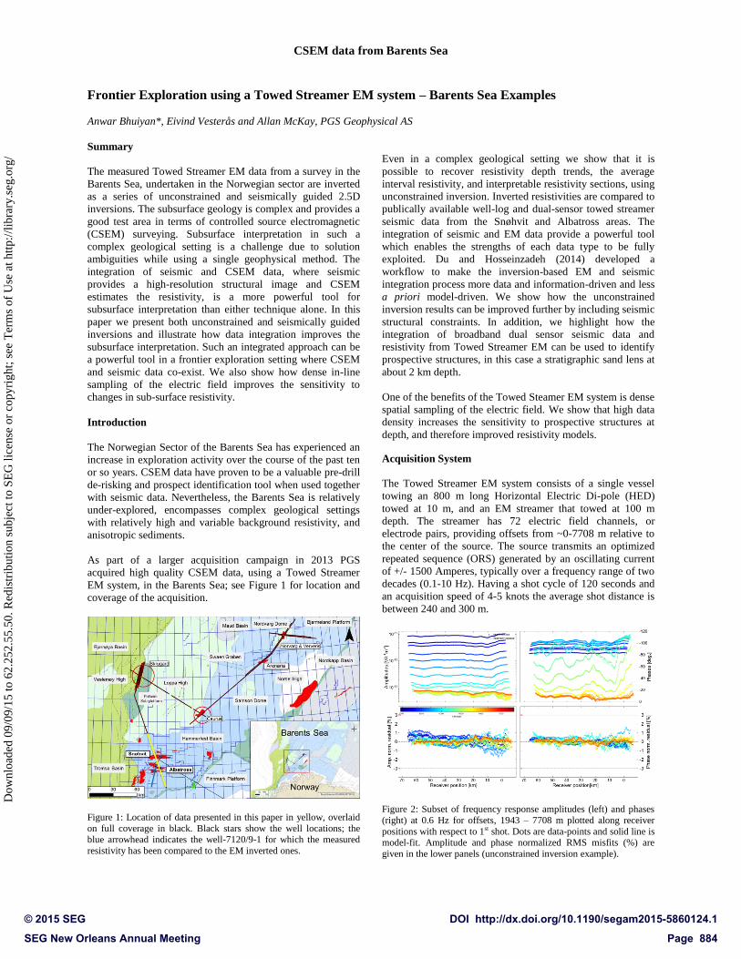
The joint analysis of Towed Streamer EM and broadband dual

sensor seismic data can reveal prospective structures. For

example, Figure 4 shows a resistivity anomaly at ~2 km depth

below sea level located ~12-15 km NW to the Snøhvit

structure. This resistivity anomaly corresponds fairly well

with seismically interpreted intra-Cretaceous sand lens

(Figure 4, lower panel). Of course further study is needed to

improve the recovered anomaly and explore the possibility

that it may be prospective.

Figure 4: Resistivity anomaly recovered by unconstrained inversion (upper panel) corresponds to intra-Cretaceous sand lens (lower

panel).

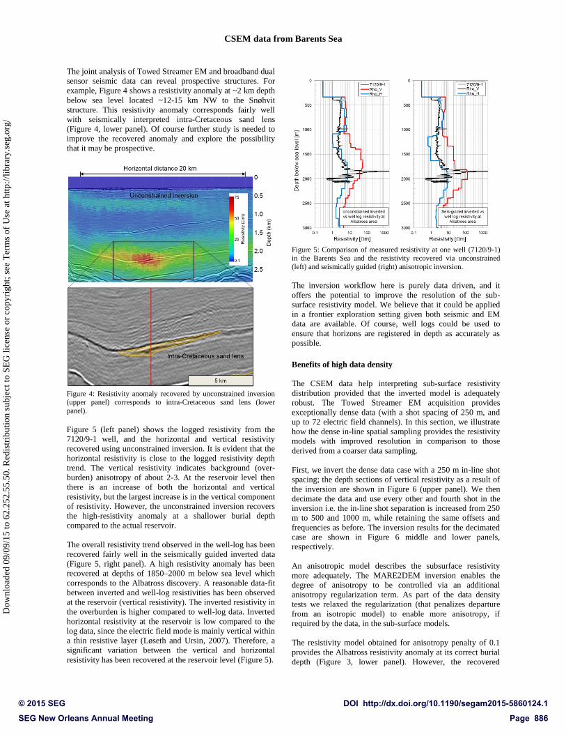
Figure 5 (left panel) shows the logged resistivity from the

7120/9-1 well, and the horizontal and vertical resistivity

recovered using unconstrained inversion. It is evident that the

horizontal resistivity is close to the logged resistivity depth

trend. The vertical resistivity indicates background (over-

burden) anisotropy of about 2-3. At the reservoir level then

there is an increase of both the horizontal and vertical

resistivity, but the largest increase is in the vertical component

of resistivity. However, the unconstrained inversion recovers

the high-resistivity anomaly at a shallower burial depth

compared to the actual reservoir.

The overall resistivity trend observed in the well-log has been

recovered fairly well in the seismically guided inverted data

(Figure 5, right panel). A high resistivity anomaly has been

recovered at depths of 1850–2000 m below sea level which

corresponds to the Albatross discovery. A reasonable data-fit

between inverted and well-log resistivities has been observed

at the reservoir (vertical resistivity). The inverted resistivity in

the overburden is higher compared to well-log data. Inverted

horizontal resistivity at the reservoir is low compared to the

log data, since the electric field mode is mainly vertical within

a thin resistive layer (Løseth and Ursin, 2007). Therefore, a

significant variation between the vertical and horizontal

resistivity has been recovered at the reservoir level (Figure 5).

Figure 5: Comparison of measured resistivity at one well (7120/9-1)

in the Barents Sea and the resistivity recovered via unconstrained (left) and seismically guided (right) anisotropic inversion.

The inversion workflow here is purely data driven, and it

offers the potential to improve the resolution of the sub-

surface resistivity model. We believe that it could be applied

in a frontier exploration setting given both seismic and EM

data are available. Of course, well logs could be used to

ensure that horizons are registered in depth as accurately as

possible.

Benefits of high data density

The CSEM data help interpreting sub-surface resistivity

distribution provided that the inverted model is adequately

robust. The Towed Streamer EM acquisition provides

exceptionally dense data (with a shot spacing of 250 m, and

up to 72 electric field channels). In this section, we illustrate

how the dense in-line spatial sampling provides the resistivity

models with improved resolution in comparison to those

derived from a coarser data sampling.

First, we invert the dense data case with a 250 m in-line shot

spacing; the depth sections of vertical resistivity as a result of

the inversion are shown in Figure 6 (upper panel). We then

decimate the data and use every other and fourth shot in the

inversion i.e. the in-line shot separation is increased from 250

m to 500 and 1000 m, while retaining the same offsets and

frequencies as before. The inversion results for the decimated

case are shown in Figure 6 middle and lower panels,

respectively.

An anisotropic model describes the subsurface resistivity

more adequately. The MARE2DEM inversion enables the

degree of anisotropy to be controlled via an additional

anisotropy regularization term. As part of the data density

tests we relaxed the regularization (that penalizes departure

from an isotropic model) to enable more anisotropy, if

required by the data, in the sub-surface models.

The resistivity model obtained for anisotropy penalty of 0.1

provides the Albatross resistivity anomaly at its correct burial

depth (Figure 3, lower panel). However, the recovered



Dow

nloa

ded

09/0

9/15

to 6

2.25

2.55

.50.

Red

istr

ibut

ion

subj

ect t

o SE

G li

cens

e or

cop

yrig

ht; s

ee T

erm

s of

Use

at h

ttp://

libra

ry.s

eg.o

rg/


Snøhvit anomaly is still inadequate compared to measured

resistivity in the well (not shown for brevity). The Snøhvit

case illustrates that relaxing the anisotropy penalty improves

significantly the recovered resistivity anomaly at the reservoir

depth (2.3 km, see Figure 6). Additionally, the recovered

resistivity anomalies at Albatross correspond precisely with

the fault segments within the structure.

Figure 6: Seismically guided inversion results showing the effects of in-line data density and anisotropy penalty regularization.

For the dense case the vertical resistivity shows a resistive

anomaly of 100-125 m at a depth of 2.1 km below the sea

level that coincides laterally with the Albatross reservoir

location (Figure 6, upper panel). There is also a layer of

slightly higher resistivity at 1500 m depth corresponding to a

contrasting lithology in the overburden. The horizontal

resistivity is somewhat lower throughout the cross section

(not shown).

If we now compare the decimated and dense cases we can see

that in the decimated case the overburden (at very shallow

burial depths) is irregular, spiky and does not look

geologically consistent. For example, there are obvious near-

surface anomalies that are not present in the dense case. In

addition, while there is still a vertical resistivity anomaly

coinciding with the Albatross reservoir it is less pronounced

compared to the dense-case scenario (Figure 6, lower panel).

In particular, we conclude that a 1000 m shot separation is too

sparse, whereas 500 m shot separation produce results

comparable to those 250 m shot separation. However, lateral

smearing is slightly higher in case 500 m separation compared

to dense-spaced samples.

The sensitivity to a change in the sub-surface resistivity

increases as the data-density increases. The left panel in

Figure 7 shows the integrated sensitivity, calculated by

summing sensitivity contribution from all frequencies and

offsets, for the 250 m shot spacing, whereas the right panel

includes the results for a data selection at every fourth shot.

Note how the increased sampling increases depth sensitivity,

especially in the region of the Albatross discovery.

Figure 7: Figure showing sensitivity variation with respect to in-line

data density. Note significantly increased sensitivity when using every shot as well as the general trend of decreasing sensitivity with

depth.

Summary & Conclusions

Seismically guided anisotropic 2.5D inversion of Towed

Streamer EM data significantly improves the lateral and

vertical resolution of resistivity anomalies obtained from

unconstrained inversion at known HC discoveries of

Albatross and Snøhvit areas in the Barents Sea. The resistivity

anomalies correspond precisely to the seismically interpreted

structures and also to the interpreted well log data at Albatross

area. By relaxing the anisotropy penalty in the seismically

guided inversion the recovered resistivity of the Albatross

structure improves noticeably and corresponds well with

individual fault segments within the reservoir. On the other

hand a high anisotropy penalty enforces horizontal

smoothness and introduces “horizontal banding” as artefacts

in the recovered resistivity models.

While guided inversion can improve the resolution we

demonstrated that unconstrained inversion can highlight

potential prospective structures e.g. a resistivity anomaly that

corresponds with a seismically interpreted intra-Cretaceous

sand lens. Thus we conclude unconstrained inversion provides

“fast track” sub-surface interpretation in frontier exploration

and also gives valuable input for parameters selection in a

structurally constrained inversion that could be used to further

define a prospect, or test hypotheses.

The high data density of a Towed Streamer EM increases the

sensitivity to changes in the sub-surface resistivity in

comparison to those derived from a coarser data sampling.

Acknowledgements

We thank Petroleum-Geo Services (PGS) for permission to

publish this work. We also thank Jens Beenfeldt and Sverre

Petlund of PGS Reservoir Services for interpreting the

broadband dual-streamer seismic data.



Dow

nloa

ded

09/0

9/15

to 6

2.25

2.55

.50.

Red

istr

ibut

ion

subj

ect t

o SE

G li

cens

e or

cop

yrig

ht; s

ee T

erm

s of

Use

at h

ttp://

libra

ry.s

eg.o

rg/

EDITED REFERENCES Note: This reference list is a copyedited version of the reference list submitted by the author. Reference lists for the 2015 SEG Technical Program Expanded Abstracts have been copyedited so that references provided with the online metadata for each paper will achieve a high degree of linking to cited sources that appear on the Web. REFERENCES

Constable, S. C., R. L. Parker, and C. G. Constable, 1987, Occam’s inversion: A practical algorithm for generating smooth models from electromagnetic sounding data: Geophysics, 52, 289–300. http://dx.doi.org/10.1190/1.1442303.

Du, Z., and S. Hosseinzadeh, 2014, Seismic guided EM inversion in complex geology: Application to the Bressay and Bentley heavy oil discoveries, North Sea: Presented at the 76th Annual International Conference and Exhibition, EAGE. http://dx.doi.org/10.3997/2214-4609.20141250.

Key, K., and J. Ovall, 2011, A parallel goal-oriented adaptive finite element method for 2.5D electromagnetic modeling: Geophysical Journal International, 186, no. 1, 137–154. http://dx.doi.org/10.1111/j.1365-246X.2011.05025.x.

Løseth, L. O., and B. Ursin, 2007, Electromagnetic fields in planarly layered anisotropic media: Geophysical Journal International, 170, no. 1, 44–80. http://dx.doi.org/10.1111/j.1365-246X.2007.03390.x.

Mattsson, J., P. Lindqvist, R. Juhasz, and E. Björnemo, 2012, Noise reduction and error analysis for a towed-EM System: 82nd Annual International Meeting, SEG, Expanded Abstracts, http://dx.doi.org/10.1190/segam2012-0439.1.



Dow

nloa

ded

09/0

9/15

to 6

2.25

2.55

.50.

Red

istr

ibut

ion

subj

ect t

o SE

G li

cens

e or

cop

yrig

ht; s

ee T

erm

s of

Use

at h

ttp://

libra

ry.s

eg.o

rg/

http://dx.doi.org/10.1190/1.1442303

http://dx.doi.org/10.3997/2214-4609.20141250

http://dx.doi.org/10.1111/j.1365-246X.2011.05025.x



http://dx.doi.org/10.1190/segam2012-0439.1

frontier exploration using a towed streamer em system ... · frontier exploration using a towed...

Documents