front page of thesis -...
TRANSCRIPT
Saurashtra University Re – Accredited Grade ‘B’ by NAAC (CGPA 2.93)
Jhala Urvashi, 2007, An Analytical Study of Financial Performance of Refinery Industry of India, thesis PhD, Saurashtra University
http://etheses.saurashtrauniversity.edu/id/eprint/50 Copyright and moral rights for this thesis are retained by the author A copy can be downloaded for personal non-commercial research or study, without prior permission or charge. This thesis cannot be reproduced or quoted extensively from without first obtaining permission in writing from the Author. The content must not be changed in any way or sold commercially in any format or medium without the formal permission of the Author When referring to this work, full bibliographic details including the author, title, awarding institution and date of the thesis must be given.
Saurashtra University Theses Service http://etheses.saurashtrauniversity.edu
© The Author

The thesis on
"AN ANALYTICAL STUDY OF FINANCIAL PERFORMANCE OF REFINERY
INDUSTRY OF INDIA."
Submitted by
URVASHI JHALA
Lecturer,
Shri V. M. Mehta College,
Jamnagar
For
Ph. D. Degree in Commerce Under
The Faculty of Commerce,
Saurashtra University,
Rajkot.
Guide :
DR. D. C. GOHIL
Head,
Department of Commerce & Business Administration,
Saurashtra University
Rajkot

Certificate This is to certify that thesis titled “ An analytical
study of financial performance of refinery Industry of
India” submitted by Ms. Urvashi N. Jhala for the award of
degree of doctorate of philosophy in commerce under the
department of commerce, Saurashtra University, Rajkot is
based on the research work carried out by her under my
guidaance and supervision. To the best of my knowledge
and belief, it has not been submitted to any other
university for the any type of degree.
Date: (Dr. D. C. Gohil)
Place: Head,
Department of Commerce
& Business Administration,
Saurashtra University,
Rajkot-360005
1

Statement of Declaration
I, the undersigned, Ms Urvashi N. Jhala, lecturer of
Shri V.M.Mehta College, Jamnagar, hereby declare that
research work presented in this is carried out under the
supervision of Dr. D. C. Gohil, Head, Department of the
Commerce and Business Administration, Saurashtra
University, Rajkot.
I further declare that the research work is my original
work and no part of this work wither fully or partly has
been submitted to and other university for any type of
degree.
Date: Researcher,
Place: (Ms. Urvashi N.Jhala)
Shree V. M. Mehta Muni.
Arts & Commerce College
Jamnagar - 361008
2

Acknowledgement
Before I move on to an in depth analysis of “An analytical study of
f inancial performance of ref inery Industry of India” I must
acknowledge my gratitude to all on whom I relied on for this research work.
First of all I am immensely grateful to my supervising guide Dr.
Daxaben Gohil (Head of the commerce department, Saurashtra University,
Rajkot) under whose scholarly guidance and supervision, I have been able to
complete my research work. Her clear perception, methodical approach, and
thorough insight into the subject have been of immense help to me in my
scholarly pursuit.
I extend my special thanks to Dr. S. J. Parmar, Reader, Department of
Commerce, Saurashtra University, Rajkot for his support and encouragement.
I am also very thankful to the staff of Department of Commerce, Saurashtra
University, Rajkot, for providing kind assistance during research period.
I am very much thankful to the staff and librarian of G.H.Gosarani
College, Jamnagar for their assistance and valuable suggestions. I am also
grateful to the staff of V. M. Mehta Municipal Arts and Commerce College,
Jamnagar for their great encouragement and support. I am also extending my
thanks to my computer operator for his accurate and speedy work.
Finally, I take this opportunity to express my gratitude to my family
members for keeping my spirit alive and supporting me during this long
period of my research work.
- Urvashi Jhala
3

PRECIS The petroleum sector is core sector for any of the country. Further
now-a- days this sector is open for free market. Energy privatization has been
part and parcel of recent trend. The industry plays a vital role in development
of economics of enterprise as well as country. So at this stage financial
appraisal of refinery industry will be very useful to many of its stakeholders.
The researcher has taken golden opportunity to analyze the financial
performance of the leading refineries.
Here, the most leading seven refineries have been taken as sample units
and the research period is from the year1998 to 2003. The thesis is mainly
based on the secondary database. Its main objectives are to evaluate the
liquidity position, working capacity efficiency level, the inventory
efficiency, debt position, profitability etc. Further, correlation of the
financial variables and other important factors that affects the financial
appraisal of the unit is used to find out in the study.
Thus, overall performance and comparison of units related to financial
appraisal are included in the study. The researcher has tried to fulfill all
objectives and to make the study useful. The study has been very useful to
the researcher to enhance the deep knowledge and experience regarding the
study.
4

CONTENTS
1 List of Tables 6
2 List of Figures 11
3 Index 13
4 Chapter-1 Research Methodology 20
5 Chapter-2 Overview of Oil Sector 40
6 Chapter-3 Sample Profile 96
7 Chapter-4 Analysis of Asset Management 127
8 Chapter-5 Liquidity Analysis 163
9 Chapter-6 Analysis of Profitability 217
10 Chapter-7 Comparison of Performance and
Evaluation of Sampled Units 268
11 Chapter-8 Summary and Findings 301
12 Abbreviations 325
13 Bibliography 328
5

LIST OF TABLES
2 OVERVIEW OF OIL SECTOR
2.1 Primary Energy Consumption
2.2 Per Capita Primary Energy Consumption
2.3 Oil Intensity
2.4 Categorization of Sedimentary Basins
2.5 PEL areas under operation by NOC’s and Pvt. / JV
Companies
2.6 ML areas under operation by NOC’s and Pvt. / JV
Companies
2.7 Indian’s Imports / Exports
2.8 India’s Crude Oil Production & Imports
2.9 Refinery Capacity Builds Up in India
2.10 Petroleum Products – Shares of different Modes of
Transport
2.11 Existing Product Pipelines
2.12 Comparison of MS Specification
2.13 Comparison of HSD Specifications
2.14 Investment Requirements in Refineries
2.15 Incremental Production Cost for MS & HSD
2.16 Long Term Demand Estimates for Petroleum Products
Consumption in India
4 ANALYSIS OF ASSET MANAGEMENT
4.4.1 Value of production to Total Assets Ratio Table
4.4.2 Value of production to Gross Fixed Assets Ratio Table
4.4.3 Value of Production to net fixed Assets Ratio Table
4.4.4 Capitals Employed Ratio Table
6

4.4.5 Value of Production to Current Assets Ratio Table
4.4.6 Value of Production to total Assets (Incr) Ratio Table
4.4.7 Value of Production to Gross Fixed Assets(Incr) Ratio
Table
4.4.8 Value of Production to Net Fixed Assets (Incr) Ratio
Table
4.4.9 Value of Production to Capital Employed (Incr) Ratio
Table
5 LIQUIDITY ANALYSIS
5.2.1 Liquidity Position of BPCL
5.2.2 Liquidity Position of HPCL
5.2.3 Liquidity Position of BRP
5.2.4 Liquidity Position of CPCL
5.2.5 Liquidity Position of KRL
5.2.6 Liquidity Position of MRP
5.2.7 Liquidity Position of IOC
5.3.1 Working Capital Investment Efficiency Test of BPCL
5.3.2 Working Capital Investment Efficiency Test OF KRL
5.3.3 Working Capital Investment Efficiency Test of CPCL
5.3.4 Working Capital Investment Efficiency Test of HPCL
5.3.5 Working Capital Investment Efficiency Test of IOC
5.3.6 Working Capital Investment Efficiency Test of MRP
5.3.7 Working Capital Investment Efficiency Test of BRP
5.4.1(A) Long Term Debt to Equity Ratio Table
5.4.1(B) ANOVA Analysis of Long Term Debt to Equity Ratio
5.4.2(A) Total Debt to Equity Ratio Table
5.4.2(B) ANOVA Analysis of Total Debt to Equity Ratio
5.4.3(A) Current Ratio Table
7

5.4.3(B) ANOVA Analysis of Current Ratio
5.4.4(A) Interest Cover (Time) Ratio Table
5.4.4(B) ANOVA Analysis of Interest Cover (Time) Ratio
5.4.5(A) Gross Working Capital Cycle (Days) Ratio Table
5.4.5(B) ANOVA Analysis of Gross Working Capital Cycle
(Days) Ratio
5.4.6(A) Net Working Capital Cycle (Days) Ratio Table
5.4.6(B) ANOVA Analysis of Net Working Capital Cycle
(Days) Ratio
5.4.7(A) Average Days of Debtors Ratio Table
5.4.7(B) ANOVA Analysis of Average Days of Debtors
5.4.8(A) Average Days of Creditors Ratio Table
5.4.8(B) ANOVA Analysis of Average Days of Creditors Ratio
5.4.9(A) Finished Goods Turnover Ratio Table
5.4.9(B) ANOVA Analysis of Finished Goods Turnover Ratio
5.4.10(A) Raw Material Turnover Ratio Table
5.4.10(B) ANOVA Analysis of Raw Material Turnover Ratio
6 ANALYSIS OF PROFITABILITY
6.2.1 (A) Z – Score Table of BPCL
6.2.1 (B) Z – Score Using the Weightage Factors of BPCL
6.2.2 (A) Z – Score Table of HPCL
6.2.2 (B) Z – Score using the weightage factors of HPCL
6.2.3 (A) Z-Score Table of BRP
6.2.3 (B) Z – Score Using The Weightage Factors of BRP
6.2.4 (A) Z – Score Table of CPCL
6.2.4 (B) Z – Score Using The Weightage Factors of CPCL
6.2.5 (A) Z – Score Table of KRL
6.2.5 (B) Z – Score Using the Weightage Factors of KRL
6.2.6 (A) Solvency Test Z – Score Table of MRP
8

6.2.6 (B) Z – Score Using The Weightage Factors of MRP
6.2.7 (A) Solvency Test Z – Score Table of IOC
6.2.7 (B) Z – Score Using The Weightage Factors IOC
6.3.1 (A) PBDIT to Gross Sales Ratio Table
6.3.1 (B) ANOVA Analysis of PBDIT to Gross Sales
6.3.2 (A) PBDT to Sales Ratio Table
6.3.2 (B) ANOVA Analysis of PBDT to Sales
6.3.3 (A) PAT to Gross Sales Ratio Table
6.3.3 (B) ANOVA Analysis of PAT to Gross sales
6.3.4 (A) PBDIT to Net Sales Ratio Table
6.3.4 (B) ANOVA Analysis of PBDIT to Net Sales
6.3.5 (A) PBDT to Net Sales Ratio Table
6.3.5 (B) ANOVA Analysis of PBDT to Net Sales
6.3.6 (A) PAT to Net Sales Ratio Table
6.3.6 (B) ANOVA Analysis of PAT to Net Sales
6.3.7 (A) Profit after Tax to Net Worth Ratio
6.3.7 (B) ANOVA Analysis of PAT to Net Worth
6.3.8 (A) Profit After Tax to Total Assets Ratio Table
6.3.8 (B) ANOVA Analysis of PAT to Total Assets
6.3.9 (A) PBIT to Capital Employed Ratio Table
6.3.9 (B) ANOVA Analysis of PBIT to Capital Employed
6.3.10 (A) PAT to Capital Employed Ratio Table
6.3.10 (B) ANOVA Analysis of PAT to Capital Employed
7 COMPARISON OF PERFORMANCE AND EVALUATION OF
SAMPLED UNITS
7.1.1 Correlation between the ratios of BPCL
7.1.2 Centroid factors for BPCL
7.1.3 Factor loadings for BPCL
7.2.1 Correlation between the ratios of HPCL
9

7.2.2 Centroid factors for HPCL
7.2.3 Factor loadings for HPCL
7.3.1 Correlation between the ratios of BRP
7.3.2 Centroid factors for BRP
7.3.3 Factor loadings for BRP
7.4.1 Correlation between the ratios of CPCL
7.4.2 Centroid factors for CPCL
7.4.3 Factor loadings for CPCL
7.5.1 Correlation between the ratios of KRL
7.5.2 Centroid factors for KRL
7.5.3 Factor loadings for KRL
7.6.1 Correlation between the ratios of MRP
7.6.2 Centroid factors for MRP
7.6.3 Factor loadings for MRP
7.7.1 Correlation between the ratios of IOC
7.7.2 Centroid factors for IOC
7.7.3 Factor loadings for IOC
8 Summary and Findings
8.1 Most Prominent Factors Of The Refinery Industry of
India
10

LIST OF FIGURE
2 OVERVIEW OF OIL SECTOR
2.1 Global Oil Consumption
2.2 Overall Indian Crude Oil Production
2.3 India’s Crude Oil Production & Imports
4 ANALYSIS OF ASSET MANAGEMENT
4.4.1 VOP/ total Assets
4.4.2 VOP/ Gross Fixed Assets
4.4.3 VOP/ Net Fixed Assets
4.4.4 VOP/ Capital Employed
4.4.5 VOP/ Current Assets
4.4.6 VOP/ total Assets (Incr)
4.4.7 VOP/ Gross Fixed Assets (Incr)
4.4.8 VOP/ GFA (Incr)
4.4.9 VOP/ Capital Employee (Incr)
5 LIQUIDITY ANALYSIS
5.2.1 Liquidity Position of BPCL
5.2.2 Liquidity Position of KRL
5.2.3 Liquidity Position of CPCL
5.2.4 Liquidity Position of HPCL
5.2.5 Liquidity Position of IOC
5.2.6 Liquidity Position of MRP
5.2.7 Liquidity Position of BRP
5.4.1 Long Term Debt to Equity Ratio
5.4.2 Total Debt to Equity Ratio
5.4.3 Current Ratio
5.4.4 Interest Coverage Ratio
5.4.5 Gross Working Capital Cycle (Days)
11
5.4.6 Net Working Capital Cycle (Days)
5.4.7 Average Days of Debtors
5.4.8 Average Days of Creditors
5.4.9 Finished Goods Turnover (Times)
5.4.10 Raw Material Turnover (Times)
6 ANALYSIS OF PROFITABILITY
6.2.1 Solvency Test Using Z-Score Analysis of BPCL
6.2.2 Solvency Test Using Z-Score Analysis of HPCL
6.2.3 Solvency Test Using Z-Score Analysis of BRP
6.2.4 Solvency Test Using Z-Score Analysis of CPCL
6.2.5 Solvency Test Using Z-Score Analysis of KRL
6.2.6 Solvency Test Using Z-Score Analysis of MRP
6.2.7 Solvency Test Using Z-Score Analysis of IOC
6.3.1 PBDIT to Sales
6.3.2 PBDT to Sales
6.3.3 PAT to Sales
6.3.4 PBDIT to Net Sales
6.3.5 PBDT to Net Sales
6.3.6 PAT to Net Sales
6.3.7 PAT to Net Worth
6.3.8 PAT to Total Assets
6.3.9 PBIT to Capital Employed
6.3.10 PAT to Capital Employed
12

INDEX
1 RESEARCH METHODOLOGY
1.1 Introduction
1.2 Identification of Problem
1.3 Significance of the Study
1.4 Review of the Existing Literature
1.5 Universe of the Study
1.6 Objective of the Study
1.7 Hypothesis
1.8 Research Design
1.9 Future Scope of the Study
1.10 Limitation of the Study
2 OVERVIEW OF OIL SECTOR
2.1 Introduction
2.2 Overall Energy Intensity and Oil Intensity
2.3 Overview of Oil Sector
2.4 Worldwide Oil Demand Growth
2.5 Need for Accelerating Energy Sector Reform Process in
India
2.6 India’s Energy Consumption
2.7 Overview of India’s Crude Oil and Petroleum Products
Scenario
2.8 India’s Exploration Scenario
2.9 New Exploration Licensing Policy (NELP)
2.10 Crude Oil Production and Imports
2.11 Overview of Demand
13

2.12 Refining Capacity Build Up In India
2.13 Deregulation of the Downstream Petroleum Sector
2.14 Petroleum Product Distribution
2.15 Petronet India Ltd
2.16 Emerging Fuel Specification
2.17 Recommended Road Map
2.18 Comparison of Indian and Worldwide MS and HSD
Quality Specifications
2.19 Investment Parameters for Up Gradation of Fuel
Quality and Vehicular Technology
2.20 Future Demand for Petroleum Products and Investment
Needs
3 SAMPLE PROFILE
3.1 Introduction
3.2 Overview of BPCL
3.2.1 Bharat Petroleum’s Mumbai’s Refineries (BPMR)
3.2.2 Refinery Modernization Project (RMP)
3.2.3 Corporate R & D Center (CRDC)
3.2.4 Financial Representation of HPCL
3.3 Kochi Refinery Limited (KRL)
3.3.1 Overview of KRL
3.3.2 Financial Representation of KRL
3.4 Chennai Petroleum Corporation Limited – CPCL
3.4.1 Overview of CPCL
3.5 Hindustan Petroleum Corporation Limited - HPCL
3.5.1 Overview of the HPCL
3.5.2 International Operations
3.5.3 Bulk Fuel & Specialities
3.5.4 Retail
3.5.5 Aviation
14

3.5.6 Financial Representation of HPCL
3.6 Indian Oil Corporation Limited – IOC
3.6.1 Overview of the IOC
3.6.2 India’s Downstream Major
3.6.3 Network Beyond Compare
3.6.4 Customer First
3.6.5 Synergy Through Subsidiaries
3.6.6 Widening Horizons
3.6.7 Mission
3.6.8 Vigilence for Corporate Growth
3.7 Mangalore Refinery and Petrochemicals Limited –
MRP
3.7.1 Overview of the MRP
3.8 Bongaigaon Refinery & Petrochemicals (BRP)
3.8.1 Overview of the BRP
3.8.2 Location and Area Covered
3.8.3 Functional Capacity
3.8.4 Capital Involved
3.8.5 Number of Manpower
3.8.6 Annual Production
3.8.7 Variety of Products
3.8.8 Required Raw Materials
4 ANALYSIS OF ASSET MANAGEMENT
4.1 Introduction
4.2 Long Term Assets
4.2.1 Tangible Fixed Assets
4.2.2 Intangible Fixed Assets
4.2.3 Investments
15

4.2.4 Other Non-Current Assets
4.3 Current Assets
4.3.1 Cash
4.3.2 Marketable Securities
4.3.3 Accounts Receivables
4.3.4 Bills Receivables
4.3.5 Stock (Inventory)
4.3.6 Prepaid Expenses and Accured Income
4.3.7 Loans and Advance
4.4 Analysis of Assets Turnover Ratio
(A) Assets Turnover Ratio
4.4.1 Value of Production to total Assets Turnover
Ratio
4.4.2 Value of Production to Gross Fixed Assets
Turnover Ratio
4.4.3 Value of Production to Net Fixed Assets Turnover
Ratio
4.4.4 Value of Production to Capital Employed
Turnover Ratio
4.4.5 Value of Production to Current Assets Turnover
Ratio
(B) Incremental Assets Turnover Ratio
4.4.6 Incremental Ratio of Value of Production to total
Assets
4.4.7 Incremental Ratio of Value of Production to
Gross Fix Assets
4.4.8 Incremental Ratio of Value of Production to
Net Fixed Assets
4.4.9 Incremental Ratio of Value of Production to
Capital Employed
16

5 LIQUIDITY ANALYSIS
5.1 Introduction
5.2 Liquidity Test
5.2.1 Liquidity test of BPCL
5.2.2 Liquidity test of HPCL
5.2.3 Liquidity test of IOC
5.2.4 Liquidity position of MRP
5.2.5 Liquidity test of BRP
5.2.6 Liquidity test of KRL
5.2.7 Liquidity test of CPCL
5.3 Working Capital Investment Efficiency Test
5.3.1 Working capital efficiency level test of BPCL
5.3.2 Working capital efficiency level test of HPCL
5.3.3 Working capital efficiency level test of IOC
5.3.4 Working capital efficiency level test of MRP
5.3.5 Working capital efficiency level test of BRP
5.3.6 Working capital efficiency level test of KRL
5.3.7 Working capital efficiency level test of CPCL
5.4 Comparative Analysis Of Liquidity Ratios
5.4.1 Long Term Debt to Equity Ratio
5.4.2 Total Debt to Equity Ratio
5.4.3 Current Ratio
5.4.4 Interest Coverage Ratio
5.4.5 Gross Working Capital Cycle (Days)
5.4.6 Net Working capital cycle (days)
5.4.7 Average days of Debtors
5.4.8 Average days of Creditors
5.4.9 Finished Goods Turnover Ratio
5.5.10 Raw Material Turnover Ratio
17

6. ANALYSIS OF PROFITABILITY
6.1 Introduction
6.2 Solvency Test
6.2.1 Z-score test of BPCL
6.2.2 Z-score test of HPCL
6.2.3 Z-score test of BRP
6.2.4 Z-score test of CPCL
6.2.5 Z-score test of KRL
6.2.6 Z-score test of MRP
6.2.7 Z-score test of IOC
6.3 Analysis of Profitability Ratios
(A) Margin Ratio
6.3.1 PBDIT to Gross Sales Ratio
6.3.2 PBDT to Gross Sales Ratio
6.3.3 PAT to Gross Sales Ratio
6.3.4 PBDIT to Net Sales Ratio
6.3.5 PBDT to Net Sales Ratio
6.3.6 PAT to Net Sales Ratio
(B) Return Ratios
6.3.7 PAT to Net Worth Ratio
6.3.8 PAT to Total Assets
6.3.9 PBIT to Capital Employed
6.3.10 PAT to Capital Employed
7. COMPARISON OF PERFORMANCE AND EVALUATION OF
SAMPLED UNITS
7.1 Introduction
7.1.1 Correlation between the ratios of BPCL
7.1.2 Centroid factors for BPCL
18

7.2.1 Correlation between the ratios of HPCL
7.2.2 Centroid factors for HPCL
7.3.1 Correlation between the ratios of BRP
7.3.2 Centroid factors for BRP
7.4.1 Correlation between the ratios of CPCL
7.4.2 Centroid factors for CPCL
7.5.1 Correlation between the ratios of KRL
7.5.2 Centroid factors for KRL
7.6.1 Correlation between the ratios of MRP
7.6.2 Centroid factors for MRP
7.7.1 Correlation between the ratios of IOC
7.7.2 Centroid factors for IOC
8 SUMMARY AND FINDINGS
8.1 Introduction
8.2 Main Findings
8.2.1 Chapter-1 Research Methodology
8.2.2 Chapter-2 Overview of Oil Sector
8.2.3 Chapter-3 Sample Profile
8.2.4 Chapter-4 Analysis of Asset Management
8.2.5 Chapter-5 Liquidity Analysis
8.2.6 Chapter-6 Analysis of Profitability
8.2.7 Chapter-7 Comparison of performance and
evaluation of sampled units.
8.3 Conclusions & Suggestions
19

CHAPTER 1
RESEARCH METHODOLOGY
1.1 Introduction
1.2 Identification of Problem
1.3 Significance of the Study
1.4 Review of the Existing Literature
1.5 Universe of the Study
1.6 Objective of the Study
1.7 Hypothesis
1.8 Research Design
1.9 Future Scope of the Study
1.10 Limitation of the Study
20

CHAPTER 1
RESEARCH METHODOLOGY
1.1 Introduction For most of the last century, firms in certain industries, especially
public utility industries such as energy, transportation, and communications,
have been public owned or regulated to alleviate public fears that such firms
would use market power to raise prices artificially. Many of these industries
exhibited scale economies, which meant that a single firm would have the
lowest cost of production and could monopolize the industry. Hence, these
industries were treated as natural monopolies and regulated to control entry,
prices, and profits.
Energy privatization has been part and parcel of a recent trend, which
has placed greater reliance on market forces and less dependence in
government in the allocation of resources. For many nations, their formerly
state owned energy companies have been among the largest of companies to
be privatized. Energy companies that have been privatized include some of
world’s largest petroleum companies based in the industrialized nations.
Global giants, such as British Petroleum, British Gas, ENI (Italy),
Petrol(Canada), Repsol (Spain), and TOTAL (France), have all undergone
transitions form state – owned to significant degree of private ownership.
Although privatization efforts differ substantially from country to
country, in general, nations have privatized state – owned energy industries
to achieve one or more of several objectives.
These objectives include:
1. Raising revenue for the state;
2. Raising investment capital for the industry or company being
privatized;
3. Reducing government’s role in the economy;
21

4. Promoting wider share ownership;
5. Increasing efficiency;
6. Introducing greater competition; and
7. Exposing firms to market discipline.
By global standards, India is just at the beginning of the energy
reforms. We however have an ideal opportunity to learn from these
worldwide experiences of the restructuring of the energy industries and put in
place the policy framework that draws from the best international practices.
This will then enable us to leapfrog into new scales of development process.
Seeing to oil sector development process, the crude oil production
shows uneven growth from 1972 to 2001. During 2000-01 230 crores of
rupees import was recorded whereas 203 crores rupees were exported by
India. It shows the gap of 2 crores rupees. Beside this, the demand of
petroleum product in India was increased every year. 1950s and the 1960s
were the years of rapid rates of increase of global oil demand, when oil
demand grew by an average of 7.7 % per year. The World’s total Primary
Energy Consumption in 2000 was 9,096 million tons of oil equivalent, and
with a world population of 6,056 million. The total investment envisaged
over the next 25 years in the downstream petroleum sector is a whopping Rs.
3, 70,000 crores or US $ 80 billion.
Energy Intensity of an economy refers to the energy consumption per
unit of GDP. The Economic growth and Energy demand are linked, however
energy intensity is influenced by the stage of the economic development of
particular economy and the standard of living of individuals.
There is an unequivocal agreement that the quality of economic
infrastructure particular, in India is a serious impediment to accelerating
growth. Energy industry is obviously one of the most critical areas.
Improving India’s energy infrastructure requires a massive increase in
22

investment in all the sub sectors. It also requires much greater levels of
efficiency to ensure low cost and good quality of service.
Thus the researcher would like to conduct the research in petroleum
industry. The study is important in views of researcher by considering
important of financial of financial analysis in profitability, liquidity, asset of
leading refineries of petroleum sector industry. The researcher will try to
shows the whole pictures of refineries and their various financial factors
which affect the industry in various financial aspects.
1.2 Identification of problem
The petroleum product and crude oil is core sector for any country.
Now a days this sector is open for free market. The main benefits for
exploring activity are fiscal incentives as a royalty and tax connection by the
government. In addition to this attractive pricing and venture capital is
another scope for the growth.
It plays a vital role in the development of economics of the enterprise
as well as country. So, the researcher would like to conduct the research on
financial aspect of petroleum industry. The main purpose of the study is to
see the basic petroleum scenario and what is the level of financial
performance of the units undertaken the study.
In modern times a number of financial problems are faced by the
industry and for effective and corrective solution of all problems, some
analytical study of the financial performance must be there.
This is a doctoral research agenda on “An Analytical study of
performance of Refinery Industries of India”.
Analytical study of financial performance turns out to be very
significant and important for the financial managers, to analyze with various
23

financial aspects. The industry uses various indicators for measuring its
financial performance. This indicates average of great importance and tells us
the true financial position of the industry.
Financial analysis report the efficiency with which the funds entrusted
to the management has been deployed. This attempts to furnish the relevant
information for its various users like creditors, bankers, financial
institutions, equity share holders, suppliers, consumers, government, etc for
their decision making. These indications help in identifying the strength and
weaknesses of the industry and suggestions.
Financial analyst depends primarily on financial statements to diagnose
financial performance. Because as long as accounting biases remain more or
less the same overtime meaningful inferences can be drawn by examining
trend and raw data in financial ratios. As well as similar biases characterize
various firms in the same industry, interfirm comparisons are useful.
If properly analyzed and interpreted, financial statements can provide
valuable insights into a firm’s performance. Analysis of financial statements
is of interest of lenders, investors, security analyst, managers, and others.
Financial statement analysis may be done for a variety of purposes which
may range from a simply analysis of short-term liquidity position of the firm
to a comprehensive assessment of the strength and weaknesses of the firm in
various aspects. It is helpful in assessing corporate excellence judging
creditworthiness, forecasting bond writing, predicating bankruptcy and
assessing market risk.
An analysis of financial statement can highlight a company’s strength
and short comings. This information can be used by management to improve
performance and by others to predicate future results. Financial analysis can
be used to predicate how such strategic decisions as a sale of a division,
major marketing program or expanding a plant are likely to affect future
financial performance.
24

So, the main purpose of the research is to be helpful to take financial
and managerial decisions by the external and internal stake holders.
1.3 Significance of the study
As earlier mentioned in the introduction the industry is core industry
and it has a very large investment of the country. So it can be said that the
large investments are blocked in the refineries undertaken for the study for
the research purpose, i t has been many reason for the significance of the
study. The significance of the study is as follows:
1) If analysis is done in various aspects like liquidity, profitability, assets
utilization, the relevant information can be furnished to its various users for
their decision making.
2) It is also necessary to find out some important factors which affect
internal decision of industry. So this research will be useful to refinery
industry itself.
3) As far as many financial and non financial institute and also government
affects by its various financial aspects, i ts various ratios should be analyzed
and the most common factors affecting refineries’ financial position should
be studied. So researcher feels its necessity and importance and therefore has
chosen this subject for her doctoral research purpose.
4) Privatization is taking place in the oil sector. So, there should not be
monopolization of any unit and competitiveness should be increased of all the
unit. To create this situation, every unit should find out their financial
position and various factors which affects to their financial condition. This
study will help to create this type of condition.
5) A large mass of the country even from housewife to businessman has
started to invest their money in the share markets. So financial analysis will
be helpful to them to take proper decision to invest their money in these
sector.
6) Petroleum is a natural product and its sources are very limited. But the
demand of petroleum product is increasing day by day. Oil demand grew by
25

an average of 7.7% per year in last few years. For this, government should
control his profitability and rate of oil prices. So if the data should be
analyses financially. Moreover profitability and other financial aspects can
be taken into the notice of this core industry.
7) Energy industry is obviously one of the most critical areas. Improving
India’s energy infrastructure requires a massive increase in investment in all
the sub sectors. It also requires much greater level of efficiency to ensure
low cost and good quality of service. So, to improve the level of efficiency
analyzed data of this research will be necessary.
8) The thesis will be a guiding path for the analysis of the study of the units
which are not undertaken for this research.
9) Saurashtra University M.phil students has undertaken the research study
by taking two refineries and tried to make financial analysis of relevant data.
So by undertaking the 7 units for the research purpose it will be the further
analysis of the industry.
1.4 Review of the existing literature
The price of petroleum product is increasing day by day. This price
rise will affect the economy as whole. The European commission forecasted
the growth of oil industry of 2005 second time in the six months 1.6% from
around 2%. predicted in October 2004 and it was due to the recorded oil cost
& unemployment with 80% in oil prices over the past twelve months and a
jobless rate of 8.9% reflecting consumer purchasing power and squeezing
corporate profits. The researcher has also studied and reviewed the following
existing literature.
The Fortune India April- 30, 2005 has focused in its cover story about
oil industry. This report includes the world crude prices, relation with a
production growth rate of oil production import and field wise crude
production in India.
26

The refinery in India is doing well but the government has created
some blocks for the growth of the sector. Indian oil industry has estimated
turnover 75 million dollar oil related market includes 30 % of India’s total
import bill . They contribute nearly 20%of the national Exchange through
customs and excise. However the country has an insignificant share (less than
1%) In the world oil and gas production, but consumption wise it accounts
for global 3%.
The Indian economy review may-2005 published by capital market
focused mainly on production prices and market capitalization. India is 3r d
largest in oil consumption after china and Japan. The current year demand
has gone up by 3.7% compare to around 4% recorded for last year. In 2004-
05 the output of refinery showed arise of 1.8%, 33981 thousand tons and
4.32% to 118216 thousand tones respectively over the corresponding period
of previous year. The OPEC country and their prices recorded highest 58 US
dollar per barrel in 2005. In India total 8 refineries have been working and
the performance is also decline.
Business India October 27, 2003 has overview the recovery growth of
various refineries. In Business India August 16,2004 covered dictions with
minister regarding oil sector.
In chartered Financial Analyst February-2005 has covered the industry
report of Indian Oil Company. The Indian Oil Company 70% of this unit
operated and control by state government. The ONGC is the largest profit
making unit and ONGC Videsh Limited operates in Iran, Syria, Myanmar,
Australia Russia etc. OVL has been major deals with 20% stock in the
Sakhalin-1 block in Russia and OVL is forint runner in investing oil and gas
field abroad. IOC is the second largest refinery and marketing company has
entered in a international field. IOC has taken biggest ever deal of 3 billion
dollar to develop a gas block to sale LPG from south Pars gas field in Iran.
This report covers the investment criteria of various companies.
27

Reliance Review of Energy Markets (December-2002) published by
reliance industry–biggest refinery having larger tons capacity of refining oil
and still expanding its project has covered full history of oil industry world
wide. It has described refinery development process since its digging age til l
today. Worldwide oil demand growth, energy consumption, crude oil
production and imports petroleum product distribution scenario, MS and HSD
quality specifications can be known from that literature. In Business Outlook
(Jan-2007) an article about Bio-fuel shows that It can also take a cue from
Brazil where the government initially bore the high cost of 100$ per barrel
(without any subsidy) in 2005-2006. With this cheaper option we may soon
see flex fuel vehicles crowding the roads. Business Standard (December
2006) presents the ranking of the 8 refineries and also presents the data of
industry wise performance.
The history shows that oil markets have highly unstable even at the
beginning of 20t h century. After the world war II, the US and Britain signed a
treaty to set up an international body which would control production and set
Prices. However the US maintained its traditional domestic price travels in
accordance with the cost of its marginal wells. Whereas the rest of the world
price was allowed to fail , this resulted in the formalist of OPEC. The book
also shows that oil prices with an upward tread for almost 30 years till the
late, 1950s after which cracks to appear.
“Refining profits” By Daksesh Parikh in ‘Business India’ (Dec.2006)
writes about the profitability of refinery Industry. According to him, given
the huge in global refining capacities most of which are running at close to
97%. Analysts expect the refining margins to stabilize at $ 6 – 8 per barrel.
The article tells that at fall capacity, the refineries will contribute Rs.20000 –
25000 crores to the top line growth depending on the crude oil price. Analyst
that even at 4 $ per barrel of refining margin the product would be making
normal profit . Thus, it shows the level of profitability is very high of each
refinery. It helps to understand the importance of profitability during the
research work.
28

“Dollar vs Oil prices – the changing equations” By N Janardhan Rao
and very in ‘The Analyst’ in Sep.2006 writes about the changing equations of
impact of dollar on oil trade. According to EMF, OPEC revenues estimated to
have gone up form $ 262 ton in 2002 to $ 61.4 bn. in 2005. Such incentives
would further encourage the oil exporting nations to increase the price of oil
in an attempt to preserve the demand of oil is increasing and will to do so
whereas an increase of in the level of global oil production appears to be
close to its maximum the OPEC oil situation countries that largely trade with
the dollar will be imported by increased energy cost.
In an article “India Sector – crude oil refineries soothing bands” in
capital market in Dec 2006, published that the petroleum E & P, refining and
allied service segment consist of industry heavy weights such as ONGC,
Indian Oil, HPCL, Bongaigaon Refinery (BRPL) and Chennai petroleum
(CPCL). The aggregates of 20 companies in the business of petroleum E & P,
refining and allied service reported a strong 39% of growth to Rs. 168029
crores in its net sales in the quarter ended Sep 2006. These sector improved
due to the accounting of oil bands.
“A study of financial appraisal of refinery units” – Varsha Virani,
M.Phil, Saurastra University has analysed the two units namely BPCL & IOC.
In her research there are various testing of hypothesis and multiple
correlation, which shows the affecting financial factors of these two units.
In Indian Journal Accounting –June 2006 issue Dr. Shantu Kumar Bose
writes the importance of oil sector. He has told that oil sector plays an
important role in refineries. They are thus catalyst for social and economic
developments in any nation. This study is an addition to these literatures for
the evaluation of the units undertaken for the study.
29

4 Universe of the study
The Universe of the study is all the leading units which are working
in refinery sector. At initial stage researcher has decided to take all the
units of the refinery sector for her research purpose but after collection of
data, researcher found that, two prominent refinery units namely Reliance
Petroleum Limited and Essar Oil Limited had not started production as
per period of study.
The following refineries which give the pictures of oil sectors of
India have been taken for the study.
1. Bharat Petroleum Corporation Ltd.
2. Hindustan Petroleum Corp. Ltd.
3. Indian Oil Corporation Ltd.
4. Mangalore Refinery & Petroleum
5. Bongaigaon Refinery & Petrochemicals
6. Kochi Refinery Limited
7. Chennai Petroleum Corporation Ltd.
5 Objective of the Study Objectives of the present study are:
1. To evaluate the fixed assets of the refineries
2. To document the profitability of the refineries
3. To evaluate the working capital situation of the refineries
4. Evaluation of Cash management of the refineries
5. Evaluation of inventory management of the refineries
6. Evaluation of debt position of units undertaken for the
study
7. Evaluation of receivable position of units undertaken for the
study.
8. To overview of overall performance of the refineries taken for
the study.
30

6 Hypothesis The hypothesis of the research has been formulated as under:
Ho: There would be no significant difference in the trend value of
production to total assets turnover ratio of all the sampled units during
period of study.
H1: There would be significant difference in the trend value of production to
total assets turnover ratio of all the sampled units during period of study.
Ho: There would be no significant difference in the trend value of
production to gross fixed turnover assets ratio of all the sampled units during
period of study.
H1: There would be significant difference in the trend value of production to
gross fixed assets turnover ratio of all the sampled units during period of
study.
Ho: There would be no significant difference in the trend value of
production to net fixed assets turnover ratio of all the sampled units during
period of study.
H1: There would be significant difference in the trend value of production to
net fixed assets turnover ratio of all the sampled units during period of study.
Ho: There would be no significant difference in the trend value of
production to current assets turnover ratio of all the sampled units during
period of study.
H1: There would be significant difference in the trend value of production to
current assets turnover ratio of all the sampled units during period of study.
31

Ho: There would be no significant difference in the trend of incremental
value of production to total assets turnover ratio of all the sampled units
during period of study.
H1: There would be significant difference in the trend of incremental value
of production to total assets turnover ratio of all the sampled units during
period of study.
Ho: There would be no significant difference in the trend of incremental
value of production to gross fixed assets turnover ratio of all the sampled
units during period of study.
H1: There would be significant difference in the trend of incremental value
of production to gross fixed assets turnover ratio of all the sampled units
during period of study.
Ho: There would be no significant difference in the trend of incremental
value of production to net fixed assets turnover ratio of all the sampled units
during period of study.
H1: There would be significant difference in the trend of incremental value
of production to net fixed assets turnover ratio of all the sampled units
during the same period of study.
Ho: There would be no significant difference in the trend of incremental
value of production to capital employed turnover ratio of all the sampled
units during period of study.
H1: There would be significant difference in the trend of incremental value
of Production to capital employed turnover ratio of all the sampled units
during period of study.
Ho: There would be no significant difference in the total debt to equity ratio
of all the sampled units during period of study.
32

H1: There would be significant difference in the in the total debt to equity
ratio of all the sampled units during period of study.
Ho: There would be no significant difference in the current ratio of all the
sampled units during period of study.
H1: There would be significant difference in the in the current ratio of all
the sampled units during period of study.
Ho: There would be no significant difference in the interest coverage ratio of
all the sampled units during period of study.
H1: There would be significant difference in the in the interest coverage
ratio of all the sampled units during period of study.
Ho: There would be no significant difference in the ratio of gross working
capital cycle all the sampled units during period of study.
H1: There would be significant difference in the in the ratio of Gross
working capital cycles all the sampled units during period of study.
Ho: There would be no significant difference in the ratio of net working
capital cycle all the sampled units during period of study.
H1: There would be significant difference in the in the ratio of net working
capital cycles all the sampled units during period of study.
Ho: There would be no significant difference in the ratio of average days of
debtors all the sampled units during period of study.
H1: There would be significant difference in the in the ratio of average days
of the sampled units during period of study.
Ho: There would be no significant difference in the ratio of average days of
creditors all the sampled units during period of study.
33

H1: There would be significant difference in the in the ratio of average days
of creditors all the sampled units during period of study.
Ho: There would be no significant difference in the ratio of finished goods
turnover of all the sampled units during period of study.
H1: There would be significant difference in the ratio of finished goods
turnover of all the sampled units during period of study.
Ho: There would be no significant difference in the ratio of raw material
turnover of all the sampled units during period of study.
H1: There would be significant difference in the ratio of raw material
turnover of all the sampled units during period of study.
Ho: Profit Before Deprecation Interest and Tax to Gross Sales ratio of all i ts
Units are same during the period of study.
H1: Profit Before Deprecation Interest and Tax to Gross Sales ratio of all i ts
Units are not same during the period of study.
Ho: Profit Before Deprecation and Tax to Gross Sales ratio of all units are
same during the period of study.
H1: Profit Before Deprecation and Tax to Gross Sales ratio of all units are
not same during the period of study.
Ho: Profit after Tax to Gross Sales ratio of all units are same during the
period of study.
H1: Profit after Tax to Gross Sales ratio of all units are not same during the
period of study.
Ho: Profit Before Depreciation Interest and Tax to Net Sales ratio of all
Units are same during the period of study.
34

H1: Profit Before Depreciation Interest and Tax to Net Sales ratio of all
Units is not same during the period of study.
Ho: Profit Before Depreciation and Tax to Net Sales ratio of all units is
same during the period of study.
H1: Profit Before Depreciation Tax to Net Sales ratio of all units is not same
during the period of study.
Ho: Profit after Tax to Net Sales ratio of all units is same during the period
of study.
H1: Profit after Tax to Net Sales ratio of all units is not same during the
period of study.
Ho: Profit after Tax to Net Worth ratio of all units is same during the period
of study.
H1: Profit after Tax to Net Worth ratio of all units is not same during the
period of study.
Ho: Profit after Tax to Total Assets ratio of all units is same during the
period of study.
H1: Profit after Tax to Total Assets ratio of all units is not same during the
period of study.
Ho: Profit Before Interest and Tax to Capital Employed ratio of all units is
same during the period of study.
H1: Profit Before Interest and Tax to Capital Employed ratio of all units is
not same during the period of study.
Ho: Profit after Tax to Capital Employed ratio of all units is same during the
period of study.
35

H1: Profit after Tax to Capital Employed ratio of all units is not same during
the period of study.
From this hypothesis, researcher would like to know the finance related
performance of all units of refinery.
7 Research design
(1) Data Collection
The study is mainly based on secondary data. The relevant information
in this regard is collected from various sources like capitalline software,
annual reports of the companies and websites. It is supported by various
articles published in various journals, business magazines. Various
researches have been referred conducted by the M.phil students and Ph,d
students of various universities. The references books have been referred
from the library of various universities. Thus, various sources have used to
collect the relevant data. No primary data has been collected.
(2) Methodology
For the financial analysis, each units first of all l iquidity position has
been tested through two ratios, current ratio and quick ratio with its graphical
representation. Every units working capital efficiency level has been tested
through debtors turnover ratio and Days Sales outstanding as well as
Inventory turnover ratio and days stock outstanding. To check the financial
leverage position, Z-score has been performed Z-score has been done by
calculating five ratios namely and then using Z-score weightage factors
methods to them. Through Z-score every units financial leverage has been
tested. Their graphical representation has been also done with its ideal
financial leverage line.
After testing every units liquidity, working capital efficiency level and
financial leverage position, their performance has been compared through
36

ratio analysis. There around 22 ratios have compared of every units. There
charts have been also presented. Further, a hypothesis have tested for the
ratio that whether there is significant difference in the ratio trend for the
period of study for the units under taken for the study. If the hypothesis is
accepted there would no significant difference in the ratio of units and if i t is
rejected, there would be significant difference in the units for the period of
study. Thus there is comparison analysis and hypothesis testing of around 22
ratios.
Thereafter, there are correlation matrixes of each unit, whereas 22
ratios have been correlates with each other and thus a table of correlation
matrix has been calculated. The table depicts the relationship among the
various ratio of profitability, asset management and liquidity. Then, there is
centroid factor analysis method of multivariable analysis has been done. Two
cnetroid factors have calculated from the correlation matrix and their
communality have been found through which parameters are most affected to
the performance of units can be highlighted. At last common variance and
eigen values have been calculated to find the percentage of common variance
from all variables can get. So percentage of loading factors and independent
variables, we can get. These variables are very useful for the units to
concentrate on the most affected variables and to improve their all over
performance.
8 Future Scope of the Study
Seven units have taken for the period 1998-2003 for the analytical
study of performance of the sampled units. The researcher has covered most
of the financial part of the sampled units. However there are more scopes for
further study as follows.
1. The researcher has taken up seven units for her study. Still financial data
can be analyzed of two prominent refineries namely Essar Oil Ltd. and
37

Reliance Petroleum Ltd. Because they were not taken up for the study as it
was not possible to collect their data pertaining to the period 1998-2003.
2. The financial aspects of these 7 units have been analyzed by performance
analysis. Still many aspects of these units such as inventory, managerial
decision, costing method, market policies, social responsibilities, human
resource management etc can be studied in future. There is a great scope for
further research in these areas.
3. This study is limited upto the period 2003. Still their financial
performance can be continued for coming years. Thus, this field is open for
further research.
9 Limitation of Study
1. Secondary data collected for the research study is collected from the
annual reports, websites and various published reports and as such finding
will depend entirely on the accuracy of such data.
2. There are different methods to measure efficiency, effectiveness and
profitability.
3. The present study is based on ratio analysis and it has its own limitation
that applies to this study also.
4. Financial statements are normally prepared on the concept of historical
cost. They do nit reflect values in terms of current cost. Thus, financial
analysis on such financial statements or accounting figures would not portray
the effects of price level changing over the period.
38

5. Financial analysis does not depict those facts which can not be expressed
in terms of money, for example- efficiency of workers, reputation and
prestige of the management.
39

CHAPTER 2
OVERVIEW OF OIL SECTOR
2.1 Introduction
2.2 Overall Energy Intensity and Oil Intensity
2.3 Overview of Oil Sector
2.4 Worldwide Oil Demand Growth
2.5 Need for Accelerating Energy Sector Reform Process In India
2.6 India’s Energy Consumption
2.7 Overview of India’s Crude Oil and Petroleum Products
Scenario
2.8 India’s Exploration Scenario
2.9 New Exploration Licensing Policy (NELP)
2.10 Crude Oil Production and Imports
2.11 Overview of Demand
2.12 Refining Capacity Build Up in India
2.13 Deregulation of The Downstream Petroleum Sector
2.14 Petroleum Product Distribution
2.15 Petronet India Ltd
2.16 Emerging Fuel Specification
2.17 Recommended Road Map
2.18 Comparison of Indian and Worldwide MS and HSD Quality
Specifications
2.19 Investment Parameters For Up Gradation of Fuel Quality And
Vehicular Technology
2.20 Future Demand for Petroleum Products and Investment Needs
40

CHAPTER 2
OVERVIEW OF OIL SECTOR
2.1 Introduction
For most of the last century, firms in certain industries, especially
public utility industries such as energy, transportation, and communications,
have been public owned or regulated to alleviate public fears that such firms
would use market power to raise prices artificially. Many of these industries
exhibited scale economies, which meant that a single firm would have the
lowest cost of production and could monopolize the industry. Hence, these
industries were treated as natural monopolies and regulated to control entry,
prices, and profits.
Energy privatization has been part and parcel of a recent trend, which
has placed greater reliance on market forces and less dependence n
government in the allocation of resources. For many nations, their formerly
state owned energy companies have been among the largest of companies to
be privatized. Energy companies that have been privatized include some of
world’s largest petroleum companies based in the industrialized nations.
Global giants, such as British Petroleum, British Gas, ENI (Italy), Petro
Canada, Repsol (Spain), and TOTAL (France), have all undergone transitions
form state – owned to significant degree of private ownership( 1 ).
Although privatization efforts differ substantially from country to
country, in general, nations have privatized state – owned energy industries
to achieve one or more of several objectives.
These objectives include:
1. Raising revenue for the state;
2. Raising investment capital for the industry or company being
privatized;
41

3. Reducing government’s role in the economy;
4. Promoting wider share ownership;
5. Increasing efficiency;
6. Introducing greater competition; and
7. Exposing firms to market discipline.
By global standards, India is just at the beginning of the energy
reforms. We however have an ideal opportunity to learn from these
worldwide experiences of the restructuring of the energy industries and put in
place the policy framework that draws from the best international practices.
This will then enable us to leapfrog into new scales of development process.
Table No 2.1
Primary Energy Consumption (Mil l ion tones o i l equivalent) )
Year North America
Central & south America
W. Europe
E. Europe
& Former USSR
Middle East Africa
Asia Pacific Other than
Japan
Japan World
1965 1,465 111 890 792 57 59 340 149 3,862 1970 1,840 145 1,151 993 73 74 460 281 5,017 1980 2,111 247 1,362 1,473 136 138 820 358 6,644 1990 2,303 321 1,491 1,715 258 219 1,391 435 8,132 2000 2,703 453 1,653 1,164 390 277 1,940 516 9,096 2001 2,640 452 1,666 1,178 397 281 1997 515 9,125 2001 share
of total
28.90% 5.00% 18.30% 12.90% 4.40% 3.10% 21.90% 5.60% 100%
(Source: - Reliance Energy Survey)
There is a table 2.1 of primary energy consumption of main countries
of world. That shows the energy consumption during the year 1965, 1970,
1980, 1990, 2000 & 2001 and the total figure of world energy consumption.
The table shows that the world’s total primary energy consumption in 1965
was 3862 million tons while it increases almost 2.5 times in the next 35
years. In 2001 was the world’s total primary energy consumption was 9125.
The region variations are very large as depicted in table 2.1. The total
42

primary energy consumption in North America in 2001 was 2640 million
tones and share in the world’s total energy consumption was 28.9%. Its shows
that North America has the highest share in world’s energy consumption
followed by Asia Pacific other than Japan which is 21.9% African region has
the least in 2001 energy consumption in the world. If is just 281 million tons
in the share of total it is just 3.1%.
Table 2.2
Per Capita Primary Energy Consumption
(KGDE)
Year North America
Central & south America
W. Europe
E. Europe
& Former USSR
Middle East Africa
Asia Pacif ic Other than
Japan
Japan World
1965 5576 537 2274 2509 986 187 202 1509 1159 1970 6515 618 2829 2999 1093 207 241 2697 1359 1980 6544 842 3143 4084 1464 295 350 3063 1500 1990 6296 899 3264 4410 1914 354 495 3524 1548 2000 6547 1079 3444 2993 2242 359 595 4059 1502 (Source: - Reliance Energy Survey)
Table 2.2 shows Per Capita Primary Energy Consumption. The primary
energy consumption translates into global average per capita energy
consumption of about 1502 kg. The regional variations are large, as depicted
in table 2.2 North American average stands at 6547 kgoe per capita while in
African region it is just 349 kgoe per capita.
2.2 Overall Energy Intensity & Oil Intensity
Energy Intensity of an economy refers to the energy consumption per
unit of GDP. The Economic growth and Energy demand are linked, however
energy intensity is influenced by the stage of the economic development of
particular economy and the standard of living of individuals( 2 ) .
The improvements (reductions) in the oil intensity of the global
economy are more pronounced than that for overall energy intensity. ( 2 )
43

Table 2.3
Oil Intensity
(KG per 1000 US $ GDP)
Year North America
Central & south America
W. Europe
E. Europe
& Former USSR
Middle East Africa
Asia Pacif ic Other than
Japan
Japan World
1965 193 181 91 959 723 162 135 73 149 1970 199 176 120 975 555 168 189 95 170 1980 166 152 101 750 342 199 248 74 156 1990 122 143 74 451 472 219 199 52 122 2000 105 143 67 277 472 213 198 48 107 (Source: - Reliance Energy Survey)
Table 2.3 shows Oil Intensity kg per 1000 US $ GDP of countries and
world. With global oil intensity (kg oil / US $ 1,000 GDP) falling from 170
kg / US $ 1,000 GDP in 1970 to 156 Kg / US @ 1,000 GDP in 1980, further it
falls to 122 kg / US @ 1000 GDP in 1990 and its 107 kg / US @ 1000 GDP in
2000. Seeing to oil intensity of countries in US there is 193 kg / US @ 1000
GDP in 1970 While in 2000 it is 105 kg per 1000 US $ GDP. While in Africa
there is 162 kg / US @ 1000 GDP and it increased to 213 kg / US @ 1000
GDP in 2000. While in other countries, oil intensity decreased in the year
2000 than 1965.
2.3 Overview of Oil Sector
Ancient Egyptians used Asphalt to embalm the mummies. Alexander,
the great used burning oil to frighten the war elephants of his enemies in 300
B.C. Marco Polo had recorded a thriving oil trade in Baku on the Caspian Sea
in the 13th century. However, the origins of the modern Oil industry are
considered to be dating back to 1859, when Col. Edwin L Drake made the
first commercial discovery of crude oil near Titusville, Pennsylvania. This
was the first reported successful ‘drilling’ opposite to ‘digging’ .
1870-72 saw John D Rockefeller forming Standard Oil Company and
monopolizing the US refining. The company dominated the US oil industry
44

for forty years but was eventually disbanded by the US Supreme Court Order
in 1911. The group broke into around forty separate companies, each
operating in one state. Of these, those in New Jersey (Exxon), New York
(Mobil) and California (Chevron) went on to become amongst the largest in
the world.
In 1877, Thomas Edison invented light bulb, and thereafter Kerosene
became marginalized by new electric il lumination. But just around the time,
another market was opening – that of automobile. In 1896, Rudolf Diesel
patented the compression engine, while Henry Ford launched the Model T car
in 1908.
Oil was first discovered in the Middle East in the early part of the
twentieth century. In the late 1920s / 1930s, a race developed to capture the
drilling rights in the Arabian Gulf. The runners in this race were obviously
the ‘Seven Sisters’ : Exxon, Mobil, Chevron, Gulf and Texaco from the US
and British Petroleum & Royal Dutch / Shell from Europe. These companies
completely monopolized the industry until the 1960s; controlling drilling,
production & refining of crude, product distribution and retailing.
For almost 20-30 years, i t appeared that all the sides of the industry
were happy, the Middle Eastern Governments happy to see their incomes
growing, and the Oil Companies enjoying high profits & increasing oil
reserves. The first signs of change appeared in 1948, when Venezuela passed
a law requiring Oil Companies to hand over 50% of their profits. The idea
quickly spread to the Middle East. Also emerging were the independent oil
companies, who began to make agreements with the Producing Governments,
offering better royalties than the Sisters. In 1951, Iran nationalized its
oilfields.
The next major important development was Suez crisis of 1956, as a
result of which the Arab states imposed an Oil embargo on the West. The
total world oil supply however was hardly affected because the production
45

increased elsewhere. In the aftermath of Suez crisis, several of the smaller
independents reached still better terms with the producers, further making
inroads into the dominance of the seven Sisters.
The Organization of the Petroleum Exporting Countries (OPEC)
was created at Baghdad in Iraq in September 1960. The rise of OPEC was
tied to a shifting balance of power from the seven sisters to the oil producing
countries. Although the essential nature of oil and the limited number of
suppliers worked in OPEC’s favour, their power remained limited during the
decade of 1960s, OPEC’s fortunes began to shift in the early 1970s, as
rapidly rising demand began to outstrip production. The 1973 oil crises has
its roots in a series of events – creation of Israel as an independent nation by
the allied powers after the World War II, refusal of Arabs to acknowledge
and the frequent attacks, the 1967 “six day war” launched by Israel and the
subsequent retaliation by Arab forces led by Egypt & Syria in 1973. To
punish the western powers for aiding the Israelis, Arab nations abruptly
halted oil exports to countries such as US and Netherlands. This came to be
known as “The First Oil Shock” .
The Second Oil Shock began with the Iranian Revolution. When the
US administration placed an embargo on the importing of Iranian oil into the
US and froze Iranian assets in response to the hostage taking, Iran
counterattacked by prohibiting the exporting of Iranian oil to any American
firm.
The Third major price spike occurred in 1990-91 when Iraq invaded
Kuwait. At the turn of the century, world oil demand is around 75 million b
/ d . The oil market in the decade of 1990s continued to be volatile and
unpredictable, seeing a price of as low as US $ 10 / bbl and a high of over US
$ 35 / bbl.
Despite these oil market volatilities and uncertainties, i t is universally
acknowledged that the 20t h century belonged to ‘oil’ . Such has been the
46

predominance of oil in meeting the global demand for primary energy. The
oil’s share in the world energy basket was 10% at the turn of the 20t h century,
packed to a level of 48% during the early 1970s and is now currently at
around 39%. During these 100 years, coil’s share has decreased from 85% to
24% from practically nil during the same period. The fact that there are lit t le
or practically no alternatives to oil’s predominance in the transportation
sector, at least the first quarter, and possibly the first half of the current
century again may well belong to oil (3 ) .
2.4 Worldwide Oil Demand Growth
1950s and the 1960s wee the years of rapid rates of increase of global
oil demand, when oil demand grew by an average of 7.7% per year. From a
level of 10.4 million b / d in 1950, the demand grew to 21 million b / d in
1960, showing a compounded growth of 7.3% p.a. and a further to 46.1
million b / d in 1970, clocking 8.2% p.a. growth.
Table 2.4
Oil Consumption Year Mllion Billion / Doller 1965 30 1968 40 1971 50 1974 55 1977 60 1980 61 1983 59 1986 60 1989 62 1992 69 1995 70 1998 71 2001 75 (Source: - Reliance Energy Survey)
47

Figure 2.4
Global Oil Consumption
01020304050607080
Con
sum
pti
Mill
ion
B /
D)
196
196
197
197
197
198
198
198
198
199
199
199
200
Year
5 8 1 4 7 0 3 6 9 2 5 8 1Oil
on
(
The figure 2.4 shows global oil demand from the year 1965 to 2001.
The oil demand was 54.4 million b / d in 1973, which fell slightly to 54.9 b /
d by 1975. Even after the first oil price shock in 1973-74, oil demand
maintained a relatively high growth rate of around 4% per year between 1975
till 1979, increasing from 54.9 million b / d to 64.3 million b / d.
The second oil shock of 1979, however, severely impacted oil demand,
due to significant shifts away from oil where substitutes were available, and
induced conservation and efficiency improvements all across the end uses of
products. Table 2.4 depicts the above matter. Between 1979 and
983, world oil demand declined from 64.3 million b /d to 57.9 million b /
nd also for industry, which lost share to coal, nuclear and
as. Since the collapse of oil prices in 1986, although fuel oil demand
ntin
petroleum
1
d or by 6.4 million b / d. Two – thirds of this decline was heavy fuel oil ,
mainly for power a
g
co ued to decline, the rate of decline slowed, while the growth in demand
for other products rose. After 1983, there has not been any significant drop in
the demand, it reached 66.3 million b / d in 1990, and by 2000 it was 75.3
million b / d.
48

2 Need for Accelerating Energy Sector Reform Process in
India
There is an unequivocal agre
.5
ement that the quality of economic
frastructure in particular, in India is a serious impediment to accelerating
rowt
Energy industry is obviously one of the most critical areas. Improving
dia’
It envisages the gas sector investment needs of US $10 billion for
r Development envisages an investment need of Rs.
00,000 crores or about US $ 165 billion in just next ten years. It’s by now
lear
ty for Petroleum and Natural Gas is not yet in
lace. Debate was on whether there should be a separate authority for
nd similarly for Petroleum segment
nd natural gas segment.
in
g h and indeed may even make it difficult to maintain the growth rates
already achieved in the 1990s.
In s energy infrastructure requires a massive increase in investment in all
the sub sectors. It also requires much greater levels of efficiency to ensure
low cost and good quality of service.
While progress has been made in India, we are stil l very much at the
beginning of this process, and much still needs to be done to catch up with
the global developments.
setting up LNG terminal, trunk gas pipelines and necessary compression
facilities for transmission and distribution of gas to the markets.
The investment needs of the Power Sector are even more daunting. The
Blueprint for Power Secto
8
c that this kind of investment needs of the energy sector greatly exceed
the resources likely to be available with the public sector.
The regulatory Authori
p
upstream and downstream or combined, a
a
The distribution reforms in the Power Sector have just begun and there
is a long way to go as the experiences till now suggest. There is thus a clear
49

case for accelerating the energy sector reform process to achieve the high
economic growth objectives.
6
r capita energy consumption was about 110 kg of oil
quivalent. By 2000, the primary energy consumption has crossed the 300
a’s Crude Oil & Petroleum Products
Scenario
at Margheritta, about
0kms from Digboi, and crude oil from Digboi was sent there by rail . The
2. India’s Energy Consumption
At the time of independence, over 70% of the total energy consumption
of India was met by the non – commercial sources of supplies like firewood,
dung cake and agricultural waste. Progressively, the situation has reversed,
with the changes in the demographic structure brought about by rapid
urbanization.
The primary commercial energy consumption in India in 1965 was
about 53 MTOE and pe
e
MTOE mark, roughly 6 times that in 1965. Population during the same period
has a lit t le more than doubled during the same period, and thus the per capita
energy consumption in India shows a 3 times jump over 1965 level, standing
today at a little over 300 kg of oil equivalent.
2.7 Overview of Indi
“DIG BOY, DIG”, shouted the Canadian Engineer, Mr. W L Lake, at
his men as they watched elephants emerging out of the dense forest with oil
stains on their feet. So the story goes about how Digboi township, in the
north – eastern corner of the country, got its name, a place that ultimately
grew into India’s as well as Asia’s first petroleum refinery and perhaps the
world’s second such outfit .
In 1889, the first commercial well was struck in Digboi at a depth of
662 ft . in 1893. AR&TC installed a tiny test refinery
2
50

pr cts included limited quantities of kerosene, lubricating oil, t imber
staining and preserving oil, iron coating oil and wax. Since AR&TC did not
have any expertise of its own in drilling and petroleum refining, it set up a
new company called Assam Oil Company (AOC) in 1889 exclusively for
taking care of its oil interest. AOC started construction of a full – fledge
petroleum refinery in 1900 and commissioned it in 1901. The products were
kerosene, wax oil for lubrication, f
odu
uel oil and grease.
f the century, till about 1956,
xploration efforts in India were limited to the Assam Arakan region. In
and accordingly, a joint venture company was
ormed, named Oil India Limited.
The resource base of hydrocarbons in India is about 29 billion tons of
il an
s of India, up to the 200m isobaths, have an areal
xtent of about 1.784 million sq. km. So far 26 basins have been recognized,
bot n l
If w
million s reased to 3.14 million sq.
km
Ind four categories, based on the
pro cti
From this beginning at the turn o
e
1956, Oil and Natural Gas Commission (ONGC) was set up by an Act of
Parliament to explore and exploit hydrocarbon reserves in the Indian
sedimentary basins. In 1958, Burmah Oil also transferred bulk of its share to
the Government of India,
f
2.8 India’s Exploration Scenario
o d oil equivalent gas. Out of this only 6.8 billion tons of the geological
reserves have been established through exploration. This leaves a substantial
resource base unexplored.
The sedimentary basin
e
h o and and offshore in this area.
e consider beyond 200 m isobath i.e. deeper waters (Area of 1.356
q. km.); the sedimentary area stands inc
. Of this nearly 41% remain yet to be explored.
ia’s basins have been categorized into
spe vely of the basins:
51

1. Established commercial production: Seven basins fall under this
ation of hydrocarbons but no commercial production
yet: Two basins fall under this category.
3. Indicated hydrocarbon that are considered geologically prospective:
Sevens basins fall under this category.
4. Uncertain potential, which may be prospective by analogy with
similar basins in the world: Ten basins fall under this category.
he categorization of India’s various basins into above categories are
as detailed in Table 2.5.
category.
2. Known accumul
T
52

Table 2.5
of Sedime B si
Basinal Area (Sq
Categorisation nt rya a ns
.Km.) Cat ory
O Offshore eg Basin
nlandTotal
Upto 2 m ISOBA 00 TH I Cambay 51000 2500 53500 Assam Shelf 56000 56000 Bombay Offshore 11 00 60 116000 Krishna Godavari 2428000 000 52000 Cauvery 25000 30000 55000 Assam - Arakan Fold Belt 60000 60000 Rajasthan 126000 126000 SUB TOTAL 0 346000 17250 518500
I I Kutch 35 000 48000 13 000 Andaman – Nicobar 000 6000 41 47000 SUB TOTAL 41000 54000 95000
I nd I I Himalayan Forela 30000 30000 Ganga 186000 186000 Vindhyan 1 1 62000 62000 Saurashtra 52000 28000 80000 Kerla-Konkan-Lakshadweep 94 000 94000 Mahanadi 55000 14000 69000 Bengal 57000 32000 89000 SUB TOTAL 542000 16 00 80 710000
I V 3 0 Karewa 70 3 0 70 Spiti-Zanskar 22000 22000 Satpur-South Rewa-Damodar 46000 46000 Narmada 17000 17000 Decan Syneclise 273000 273000 Bhima-Kaladgi 8500 8500 Cuddapah 39000 39000 Pranhita-Godavri 15000 15000 Bastar 5000 5000 Chhattisgarth 32000 32000 SUB TOTAL 461200 461200
TOTAL 1390200 394500 1784700 DEEP WATERS (Kori-Comorin 85 E Narcodam) 1350000
GRAND 3134700 TOTAL (Source: - Reliance Energy Survey)
The sedimentary basins covering Assam, Gujarat, Rajasthan, Bombay
High, Krishna – Godavari and Cauvery fall in Category I, from where oil and
Gas is produced commercially. There is no commercial production from the
53

other sedimentary basin areas that constitute almost 83% of the entire
sedimentary area, and fall in Category 2, 3 or 4.
Mining Lease (MLs) and the block awarded up to NELP 2. Balance 1.18
million sq. km are presently not nder any PELs / MLs/ awarded
block
Of the 1.356 million sq.km of at as, so far 0.272 million
sq. km is covered under va PEL / b awarded up to NELP 2.
The remaining 1.084 million sq. km a vaila for future coverage.
ab
PEL areas under by and t. / JV Companies
a
Of the total basin area of 1.78 million sq. km up to 200 M isobath,
about 0.6 million sq. km include the areas held by National Oil Companies
and private companies through Petroleum Exploration Licenses (PELs) /
covered u
.
deep – w er are
rious s / MLs lock
rea is a ble
T le 2.6
operation NOC’s Pv
PEL Are Company (S ) q. Km (%)
ONGC 3 08,786 52% RIL 99,980 17% OIL 4 4,554 8%
HOEC 3 7,212 6% CAIRN 26,044 4% ESSAR 21,905 4%
OKLAND 18,783 3% GAZPROM 10,425 2% PHOENIX 6,928 1% TULLOW 5,131 1% HARDY 5,091 1% ENRON 3,209 1% ASSAM
CO. 1,800 0%
ENPRO 300 0% TOTAL 590,228 100%
(Source: - Reliance Energy Survey)
Tables 2.6 indicate petroleum exploration licenses areas (PELs) under
operation by National Oil Companies and private / joint venture companies.
Under Petroleum Exploration lice panies are under operation. nses 14 com
54

The table 2.6 shows that total 590228 sq km areas are for PELs. Among
them ONGC has the maximum 308786 sq. km Ls which is 52% of the
total share followed by RIL as 17% 99 q km areas. While the
Essar has 21905 sq km areas and has onl o re of total PEL area.
Thus ONGC has covered lar a of pet exploration.
able 2.7
ML areas under operation by NOC’s and Pvt. / JV Companies
Are
areas PE
which h and 9 80 s
y 4% f sha
gest are roleum
T
ML a Company (
KmSq.
) (%)
ONGC 8, 145 54% OIL 3,239 22%
ENRON 2,678 18% CHIRN 333 2% NIKO 229 2%
SELAN 171 1% MOSBACHER 75 1%
L&T / JTI 57 0% HOEC 15 0%
GEOENPRO (GEOEN.) 11 0%
INTERLINK 4 0% TOTAL 14,957 100%
(Source: - Reliance Energy Survey)
Table 2.7 indicate mining lease area under operation by National Oil
ompanies and private / joint venture companies under mining lease eleven
mpa
a, ONGC company has 8145 59 km areas for ML
Oil
ompanies on nomination basis, availability of exploration areas was assured
C
co nies are under operation.
Above table shows that total 14957 59 km areas was there for mining
lease (MLs) out of total are
which is 54% of the total share – followed by Oil which has 3239 59 km
areas for MLs and has 22% of total area ESSAR company had no MLs areas.
Under the previous system of awarding acreage to National
C
and the estimation of the quantum of the future work to be undertaken was
relatively straightforward.
55

The new system of award of blocks through competitive bidding has
introduced a large element of uncertainly. Further, since most of the
vailable areas are totally virgin, significant efforts are required to build the
in the past as the
emaining frontiers are expected to be technologically and geologically more
xploration Licensing Policy (NELP) was announced by the
overnment of India in March 1997. It introduced a level playing fields
nies were required to compete with
e Private and the Joint Venture companies, in acquiring exploration
acreag
would tted work program, profit petroleum share
e c
recove
Salie
i .
i i . taining the petroleum exploration
a
geological knowledge base through aggressive data acquisition programs.
The risk – reward framework in most of the new E&P activities in
India is thus likely to be much more challenging than
r
complex and logistically more difficult.
As the sector moves into the free market scenario, the main drivers for
exploration activity would be fiscal incentives in the form of royalty and tax
concessions, more elaborate and attractive data packages, attractive pricing
for the crude produced and availability of venture capital.
2.9 New Exploration Licensing Policy (NELP)
New E
G
concept, wherein the National Oil Compa
th
es in Indian sedimentary basins. Under this policy, the Companies
be required to bid for commi
xpe ted and % of annual production sought to be allocated towards cost
ry(4 ) .
nt Features of NELP in India
There is no Mandatory State participation through ONGC / OIL nor any
carried interest of State.
ONGC and OIL to compete for ob
licenses on competitive basis instead of granting them petroleum
56

exploration licenses on nomination basis. ONGC and OIL will get same
fiscal and contract terms as available to private companies.
be charged
bathymetry for the first 7 years after
vii . h was earlier levied on crude production, has been abolished
port duty on the goods
imported for petroleum operations.
There are no signature, discovery and productions bonuses.
x. A seven – year tax holiday is available from the date of commencement
of commercial production.
Contractor is provided fiscal stability during the entire period of
contracts.
i i . A separate Petroleum Tax Guide is in place to facilitate investors.
xiii . A revised model contract is in place.
i i i . Open availability of exploration acreages to provide a continuous
window of opportunities to oil companies. The acreages will be
demarcated on a grid system and pending preparation of the grid,
blocks will be carved out for offer.
iv. Freedom to the contractors for marketing of crude oil and gas in the
domestic market.
v. Royalty payments at the rate of 12.5% for the onland areas and 10% for
offshore areas.
vi. To encourage exploration in deep water areas, royalty will
at half the prevailing rate for normal offshore area for deep – water
area beyond 400 meter
commencement of commercial production.
Cess, whic
for the blocks offered under NELP.
viii . Companies are exempted from payments of im
ix.
xi.
x
57

2.10 Crude Oil Produc nd Imp s Table 2
Overall Crude Oil Production Production in
MMTPA
tion a ort.8
Indian
Year 1970-71 7 1972-73 8 1974-75 8 1976-77 9 1978-79 12 1980-81 11.5 1982-83 10 1984-85 24.8 1986-87 30 1988-89 29.9 1990-91 35 1992-93 29 1994-95 29 1996-97 36 1998-99 33 2000-01 34
(Source: - Reliance Energy Survey)
Figure 2.8
Overall Indian Crude Oil Production
05
1015
1970
-71
1972
-73
1974
-75
1976
-77
1978
-79
1980
-81
1982
-83
1984
-85
1986
-87
1988
-89
1990
-91
1992
-93
1994
-95
1996
-97
1998
-99
2000
-01
YEAR
Prod
uc
2025303540
tion
in M
MTP
A
Series1
Table 2.8 shows the overall Indian crude production from the year
1970-71 to 2000-01. Before the Bombay High Offshore discovery, the crude
oil production in the country was less than 10 million tons per annum. The
58

crude
stagnated at about 32 million tons per
year.
With crud illion tons per
year, along with massive re capacity addition replacing product imports
with crude, and nd gr ng rapidl the impo of crude oil have
rapidly increase t f years.
Table 2
s Crude Oil Production and Imports
TPro ion Im ts
TAva lity
oil production in the country increased rapidly in the 1980s. It was
around 34 million tons in 1989-90. It fell to about 27 million tons in 1992-
93. The country’s production achieved an all t ime peak of 35 million tons in
1995-96. Thereafter the production has
e oil production stagnating at around 32 m
fining
dema owi y, rts
d in the las ew
.9
India’
Year otal
duct porotal
ilabi1970-71 8 15 20 1972-73 8 15 20 1974-75 9 18 21 1976-77 9 17 21 1978-79 10 17 22 1980-81 9 17 22 1982-83 20 19 30 1984-85 30 18 41 1986-87 33 18 42 1988-89 34 20 45 1990-91 33 20 55 1992-93 25 27 56 1994-95 34 25 60 1996-97 33 33 61 1998-99 32 33 68 2000-01 33 75 105
(Source: - Reliance Energy Survey)
59

Figure 2.9
India's Crude Oil Production & imports
0
20
120
1
40
60
80
MM
T
00
-71
-73
-75
-77
-79
-81
-83
-85
-87
-89
-91
-93
-95
-97
-99
-01
PA Total ProductionImportsTotal Availability
1970
1972
1974
1976
1978
1980
1982
1984
1986
1988
1990
1992
1994
1996
1998
2000
Year
Table 2.9 shows trend of
quantity of crude oil imported was about 34 m
India’s crude oil production and Imports. The
illion tons each in 1996-97 and
1997-98. It increased to about 40 million tons in 1998-99, about 58 million
tons in 1999-00 and 74 e period
product imports have dropped down from 22.23 million tons in a year to
about 9 million tons in 2000-2001 and furthe to 6.5 m tons in
2001-02.
e s su nc il ov dra ical allen
from re than 80% in 1984-85 to in -91 ju out % in
2000- .In ter he oi ort e o S 4 bi n, or
Rs. 1 37 in -9
implications on the Trade balance for the
country. In 2000-01, the overall trade balance was –ve US $ 6 billion.
However, the balance on ac
million tons in 2000-01 during the sam
r down illion
Th elf – fficie y in o has, er the years, mat ly f
mo 64% 1990 , and st ab 31
01 value ms, t crude l imp s wer ver U $ 14. llio
8,3 crores 1996 7.
These have considerable
count of oil and petroleum products was –ve US $
13.8 billion. Thus, excluding oil and petroleum products, there was a trade
surplus of US $ 7.8 billion.
60

Table 2.10
Indian’s Imports / Exports
Total Oil Imports Exp Imports Exports orts
year Rs. Crores $
MM Rs. Crores MM Rs. Crores $ MM Rs. Crores $
MM $
92 63375 21882 53688 18537 17142 6100 1379 473 93 73101 23306 69751 22238 18046 5754 1248 398 94 89971 28654 82674 26331 18613 5928 1809 417 95 122678 36675 106353 31795 25174 7526 1518 454 96 138920 39132 118817 33470 35629 10036 1710 482 97 154176 41484 130101 35006 30341 8164 1311 353 98 178332 42389 139753 33219 26919 6399 376 89 99 215236 49671 159561 36822 54649 12611 168 39
2000 230873 50536 203571 44560 71497 15650 8542 1870 (Source: - Reliance Energy Suryvey)
Above table indicate India’s imports and exports from 1992 to 2000.
Total imports in 1992 was 63375 crores and 21882 $ MM. Oil imports in
1992 was Rs. 17142 crore and 6100 $ MM. Total exports in 1992 was Rs
53688 crores and 18537 $ MM and oil exports was Rs 1378 crores and 473 $
MM. Total imports indicates increasing trend during 1992 to 2000. Whereas
oil imports and exports shows flu d.
able 2.11
ctuating tren
T
10
20
01st Qtr 2nd Qtr 3rd Qtr 4th Qtr
30
40
50
60
70
80
90
100
EastWestNorth
61

Table 2.12
Oil Production & Imports
Year Total
Production Imports Total
Availability
India’s Crude
1991-92 30.3 24.0 54.3 1992-93 27.0 29.2 56.2 1993-94 27.0 30.3 57.8 1994-95 32.2 27.3 59.6 1995-96 35.2 27.3 62.5 1996-97 32.9 33.9 66.8 1997-98 33.9 34.5 68.4 1998-99 32.7 39.8 72.5 1999-00 31.9 57.8 89.8 2000-01 32.4 74.1 106.5 (Source: - Reliance Energy Suryvey)
Table 2.12 and the chart above indicate the total production, imports
and total availability from 1991 to 2001. Total production in India in 1991
was 30.3 million tons and imports 24 million tons. So total availability was
54.3 million tons In India total production is not constant. So total
availability shows increasing trend during the period 1991 to 2001
e overall demand for petroleum products in India grew an average of
bout 5.8% in 1990s, and the 1980s, and 5.3% p.a. in the 1970s. From a level
the 1970s. During the late 1990s, Naphtha consumption has increased two
esult
f Liquid Fuel Policy and switchover by many fertilizer units to Naphtha, due
2.11 Overview of Demand
Th
a
of just 18 million tons in 1970-71, the demand for petroleum products
reached 50 million tons in 1988-89 and 100 million tons in 2000-01.
The elasticity of the demand for petroleum products with respects to
GDP was about unity in the 1900s, while it was 1.2 in the 1980s ad nearly 2
in
and a half times, from 4.7 million tons in 1996-97 to 11.7 million tons in
2000-01, principally due to the commissioning of India’s largest Naphtha
Cracker of Reliance, host of naphtha based power plants allowed as a r
o
to inadequate gas supply.
62

HSD, which currently accounts for 37% of the total petroleum product
man
hen
verall petroleum product consumption was actually lower than the previous
few years. The last –ve growth was in 1974-75, when
onsumption fell by 0.24 million tons with respect to the previous year.
government ownership as a
esult of the merger of two government owned companies, which were
stabl
ons, in 1974-75. While
refining capacity grew from 28 MMT A in 1975 to 52 MMTPT by early
de d, grew at a CAGR of 6.4% in the 1990s. LDO (nil), ATF (2.8%), Fuel
Oil / LSHS (3.3%) and SKO (3.5%) had lower growth rates, during the same
period.
The year 2001-02 was the first year, after twenty-seven years, w
o
year. In 2001-02 the consumption fell by 1.5 million tons with respect to
2000-01. HSD (-1.3 million tons) accounted for the bulk of the fall , which
was partly recouped by LPG (+0.7 million tons) and MS (+0.4 million tons).
The FO / LSHS consumption has remained stagnant at about 12.5
million tons in the last
c
2.12 Refining Capacity Build Up in India
At the time of independence, there was only one refinery in India,
located at Digboi, with a capacity of just 0.25 million tons per annum. In the
late 1950s and early 1960s refineries were set up with the assistance of
international oil companies such as Shell, Caltex and Esso, which after
nationalization, become BPCL and HPCL Vizag / Mumbai respectively( 5 ).
Indian Oil was formed in 1964 with 100%
r
e ished in the late 1950s. Cochin Refineries Limited and Madras
Refineries Limited were set up in the 1960s by the Indian government in
association with Philips Petroleum, and Amoco, and National Iranian Oil
Company respectively.
At the time of nationalization of the refining and the marketing sector,
the refining capacity in India was around 28 million t
P
63

1990s, with only one new grassr y and the rest through capacity
expansions, the con . From negligible
quantum, during mid 1970s, the product imports grew to around 12 m on
ton e s l n . te
1990s. In the decade of s, n sec r as pro ively
de le it b eni u ri sector, culminatin o the
rem f n ed e m an
i fi c ty eas 6 fro o 8 m tons
pe n - ly 112 mi t n 01, y 43
MM ar ith lia s M ries
ontributing a large chunk of this increase. This has made the country self
oots refiner
sumption outpaced the capacity addition
illi
s in th early 0199 pand ac aked t over 2 il0 m io ton s p.a in / lamid
1990 refi ing to w gress
control d, in ially y op ng it p to p vate g int
oval o admi ister pric ech ism.
Ind a’s re ning apaci incr ed by 4% m ar und 6 illion
r year i 1998 99 to approximate llion ons i 2000- i .e. b
TPA, in just two ye s w Re nce’ 27 MTPA refine
c
sufficient in refining capacity, significantly improving the energy security
and domestic value addition. Product imports have virtually stopped, thus
saving the precious foreign exchange for the country.
Table 2.13
Refinery Capacity Builds Up in India
(KT)Year IOC BPCL BRPL KOCHI HPCL CPCL MRPL RIL ALL INDIA
1991-92 24400 6000 1350 4500 10000 5600 51850 1992-93 24400 6000 1350 4500 10000 6500 52750 1993-94 24550 6000 1350 7500 10000 7000 53400 1994-95 24550 6000 1350 7500 10000 7000 56400 1995-96 24550 6000 1350 7500 10000 7000 56400 1996-97 24550 6000 2350 7500 10000 7000 3000 60400 1997-98 25700 6000 2350 7500 10000 7000 3000 61550 1998-99 31700 6000 2350 7500 10000 7000 3000 67550 1999-00 35600 6900 2350 7500 13000 7000 9690 27000 112040 2000-01 36100 6900 2350 7500 13000 7000 9690 27000 112540 2001-02 38150 6900 2350 7500 13000 7000 9690 27000 114590 (Source: - Reliance Energy Suryvey)
Table 2.13 indicates refining capacity build up in India for the year
1991-92 to 2000-01 of all refineries. 6000 million tons refining capacity
build up in BPCL for the year 1991 to 1999. On the other hand in IOC
refining capacity shows increasing trend. Highest refining builds up in 2000-
01 with 36100 million tons. BRPL has 1350 million tons refining capacity till
64

1995-96 but then it increased to 2350 since 2001-02. KOCHI has 7500
finin
pect of the oil industry was highly regulated after the
ationalization of these assets( 5 ) .
steps were taken to attract the private sector. The
efining sector was opened up to the private sector in 1991.
re g capacity till 2000-01. Refining capacity of HPCL increased from
10000 million tons to 13000 million tons in 1999-00. CPCL has the same
refining capacity of 7000 million tons from 1992-93 to 2001-02. MRPL
refinery started from 1996-97 and its refining capacity was 9690 million tons
in 2001-02. and at last RIL refinery set up in 1999-00 but it has second
highest refining capacity of 27000 million tons till 2001-02. IOC has highest
refining capacity compared to all other refineries.
2.13 Deregulation of the Downstream Petroleum Sector
The oil shocks of the mid – 1990s saw the nationalization of the
downstream petroleum sector. While Esso was nationalized in 1974, Caltex
and Burmah – Shell were nationalized in 1976. IBP was nationalized in 1972.
Almost all as
n
Up to the run up till 1990, only one refinery was set up in the country
and with no major oil discoveries after 1986s, India’s dependence on
imported crude and petroleum products increased substantially. It was felt
necessary to attract private and foreign investment to augment India’s
refining capacity, domestic oil reserves and production. With the onset of the
economic reforms in 1990s,
r
In April 1993, the Government decimalized imports of LPG, Kerosene
and LSHS. The government allowed importing and marketing of LPG and
kerosene by the interested parties under the Parallel Marketing Scheme by
amending the relevant control orders in August / September 1993. Similarly,
Government allowed direct imports of LSHS by the parties for captive
consumption.
65

The lubricant marketing was completely deregulated since November
1993. In January 1995, Ministry of Petroleum and Natural Gas appointed a
Strategic Planning Group on Restructuring of Oil Industry to make
recommendations to meet the policy objectives and initiatives required for
restructuring the oil industry. The R – Group recommended the gradual
phasing out of Administered Pricing Mechanism (APM) and introduction of
ee marketing mechanism.
M in
hases starting from 1s t April 1998, with full deregulation envisaged by
he second
eport dealt with phased dismantling of APM suggesting appropriate duty
From 1s t April 2002, the administered price mechanism has been
sma
estic LPG and Kerosene for
ublic distribution is expected to continue for next three to five years and
Oil Pool Account has been
fr
Based on the recommendations, the Government issued the Gazette
notification I November 1997 delineating the path to dismantle the AP
p
March 2002. In June 1996, MOPNG constitute an Expert Technical
Group (ETG) to examine the impact on various sectors at different level of
duty structure in case of dismantling of APM, as recommended by the R –
Group.
The first interim report had made recommendations on tariffs on
capital goods, which were implemented in a modified manner. T
r
structure within the constraints of the prevailing pool deficit . In accordance
with the recommendations, a phased program of duty rationalizations is being
implemented since April 1998.
In the third and the final report of ETG, the Group had examined
pipeline tariffs, for crude and products, and compensation mechanism for
marketing operations. In June 1998, the refining sector was delicensed.
di ntled and oil – marketing companies are being allowed to fix retail
prices for MS and HSD. The subsidy on dom
p
will be borne by the Union Budget. The
66

disma
t h April 2002, the Union Cabinet cleared the bill for setting up
the Petroleum Refining and Marketing Regulatory Board, and on 6t h May,
2002,
e
petrol m products are available throughout the country by imposing retail
servic
ndia has one of the most extensive rail networks in the world, and rail
movem
st of transportation through rail increases
annually because of the higher operating cost as against pipelines whose
operat
leum
ntled and the Government issued Oil Bonds worth Rs. 9,000 crores to
oil companies against their outstanding with the Oil Pool Account.
On 18
it was introduced in the Parliament. The Board is expected to monitor
petroleum product prices in the deregulated scenario and ensure that there is
no profiteering by the Oil Marketing Companies. It will also ensure that th
eu
e obligations for existing and new oil marketing companies. At present,
the Bill is with the Parliament Standing Committee on Petroleum.
In May 2002, Government granted marketing rights to Reliance,
Numaligarth Refineries, ONGC and Essar Oil.
2.14 Petroleum Products Distribution
I
ent of petroleum products is still one of the major modes of
transportation, accounting for 35% of the total product distribution
movement.
The railways are facing increasing constraints in movement of oil non
– availability of locomotives and tank wagons, due to resource constraints,
and hence the share of the railways has been steadily decreasing over the past few years.
Over the long run, the co
ing costs are minimal. The freight rates of railways in India have also
been distorted due to the cross subsidization of passenger traffic by freight
traffic and of other special products being transported. Even though this
cross – subsidy is expected to decrease over time, rail transport for petro
67

products is expected to be stil an pipeline transport, thereby
resulti
ta o rol products by roads
c ute u 0% e to tran at M ent of products
fr ep te als tail ts ed he oxi is d
only through road alternate m
H er, usage of roads for long haul transportation is increasingly
becom ng safety hazard. This is owing to the increase in number of vehicles
on roa nditi highways coupled with
ve es re ma ed p erly d , who are d to
la i sk
h r short ge et tr uct ere
is need for accelerated development of pipelines to
eet
Table 2.14
l costlier th
ng in a higher overall cost for the consumer, especially vis-à-vis pipelines.
Currently, the transpor tion f pet eum
ontrib s aro nd 3 of th tal sport ion. ovem
om d ots / rmin to re outle situat in t ir pr mity one
transportation as odes would be unviable.
owev
i
the d, poor co ons of national and state
hicl that a not intain rop and rivers foun be
cking n safe driving ills.
W ile fo haula of r ail pe oleum prod s, th no
substitute for roads, there
m the bulk transportation needs. The shares of different modes of
transportation of petroleum products in the 1930s are as detailed in Table 2.14
Petroleum Products – Shares of different Modes of Transport
Road Rail Pipel ines Coastal Total POL Road Rail Pipel ines Costal
Year MMT MMT MMT MMT MMT % % % %
1993-94 15.3 26.1 14.5 4.9 60.8 25% 43% 24% 8%
1994-95 17.9 28.1 14.9 4.6 65.5 27% 43% 23% 7%
1995-96 22.2 29.3 15.2 5.5 72.5 31% 40% 21% 8%
1996-97 23.1 29.1 19.1 5.8 77.1 30% 38% 25% 8%
1997-98 22.2 31.8 21.1 9.2 84.3 26% 38% 25% 11%
1998-99 25.4 33.2 23.9 8.3 90.8 28% 37% 26% 9%
1999-00 22.39 35.1 27.8 9.6 95.4 24% 37% 29% 10%
2000-01 23.9 37 31.5 9 23% 36% 31% 10% 10.6 102.
2001-02 24.09 36.4 35% 30% 11% 31.6 11.6 104.4 24%
(Source: - Reliance Energy Survey)
68

The table 2.14 indicates petroleum products – shares of difference
mod ransportat the year 1 to of
transp include and c l.
e table 995-96 a f r an for
petroleum produ 25%, t hare of
the sh of pipe as 24% coastal trans e
share of road tran in 1995-96 up to 31% but it ease
to 24% the ye share o l tran t de s t in
the ye 001-02 ip ransport for pe um pr t
8% to 11% in 2001-02. Petroleum products by
oads shows fluctuating trend where in the other modes of transport shows
ncrea
lines
Sr
Year
e of t ion for 993 2002. Different modes
ort road, rail , pipeline osta
Th shows that in 1
stribution
the sh re o oad tr sport
ct di was he s rail transport was 43%,
are line transport w and port was 8%. Th
s port increased again decr
in ar 2001-02. The f rai spor crease o 35%
ar 2 . Whi share of ple the eline t trole oduc
distribution increased from
r
i sing trend. The transportation of petroleum products by rail consist
highest share.
Table 2.15
Existing Product Pipe
.No. Pipel ine Length
(km) Capacity
(MMTPA) Owner of
Comm.1 Guwahat i - Si l igur i 435 0.8 IOCL 1964 2 Koyal i - Ahmedabad 116 1.1 IOCL 1966 3 Barauni - Kanpur 69 1.8 IOCL 1966 4 Haldia - Barauni 525 1.4 IOCL 1966
5 Haldia - Mourigram - Rajbandh 269 1.3 IOCL 1974
6 Mathura - Jalandhar 526 3.7 IOCL 1982 7 Kandla - Bhat inda 1443 6 IOCL 1996 8 Mumbai - Pune 161 3.9 HPCL 1985 9 Digboi - Tinsukhia 75 0.7 IOCL
10 Mumbai - Manmad 252 4.3 BPCL 1998 11 Visakh - Vijaywada 356 4.1 HPCL 1998 Total 4 ,827 29
(Source: - Reliance Energy Survey)
India has a pipeline network of around 5000 Kms for the transportation
of petroleum products from the refineries to the consumption centre. BPCL
own a 250 – Km pipeline and HPCL owns two pipelines, totaling around 500
69

kms…The rest is owned by IOCL. The details of the product pipelines
urren
stly cater to the west to north – west
Maharastra, Gujarat, Rajasthan, Punjab, Haryana, Delhi, and western Uttar
east (West Bengal, Bihar, and eastern Uttar
radesh) corridors. The south has only one pipeline, from Visakhapatnam to
ted under the Administered
ricing Mechanism on a retention basis. The unit rate is determined for each
eregulated scenario, the market would determine the
ost cost effective and efficient mode of transportation, pipelines, with their
bviou
.15 Petronet India Ltd.
VK Ltd.
re owned by the three PSUs, the future product pipelines are proposed to be
set
by In
c tly under operation are as per Table 2.15
The above table shows that most of these pipelines are concentrated in
the west to north – west (around 55%) and east to north sectors (40%).
Therefore, these pipelines mo
(
Pradesh) and east to north –
P
Vijaywada.
Currently, the pipelines are compensa
P
pipeline by dividing total operating cost and return on capital by the standard
throughput of the pipeline. Standard throughput was considered at 80%
capacity utilization earlier. In 1994-95, the government decided to adopt 95%
capacity utilization for existing pipelines and around 70% for the initial two
to three years for new pipelines.
The pipelines offer numerous advantages over the competing modes of
transport. While in the d
m
o s advantages, are expected to play a major role in future transportation
of petroleum products in India.
2
While the existing pipelines, with the exception of Petronet
a
up by Petronet – Joint Venture Companies.
Petronet India Limited (PIL) is a financial holding company promoted
dian Oil Ltd. (IOCL), Bharat Petroleum Corp. Ltd. (BPCL) and
70

Hindu
the G troleum product
pipelines to meet the demand of petroleum products in the country by
expeditious implementation of the pipeline projects and to form an
org
oil co
IBP (2
(10%)
advan rt as enumerated below:
1.
of transportation only the
by pipelines is only 40% of that for
2.
.3 -0.5% losses.
g and coordination which could
lead to delays and losses.
5. Pipelines are more environme t friendly mode of transportation.
Further, since they are laid below the ground, land can be restored to
its original use unlike other modes.
stan Petroleum Corp. Ltd. (HPCL). It was formed under a directive of
overnment of India with the objective of laying pe
anization capable of funding and minimizing the limitations of individual
mpany.
The present equity holders are IOC (16%), HPCL (16%), BPCL (16%),
%), IL&FS (10%), ICICI (10%), SBI (10%), Reliance (10%) and Essar
.
Transportation of Petroleum Products by Pipeline has several
tages over the other modes of transpo
For bulk transportation, pipelines are most energy efficient, cost
effective and convenient. In this mode
product moves whereas the contained remains stationary unlike the
other modes. The estimated energy consumption for movement of
petroleum products per MT per Km
rail and less than 10% of that for road transportation.
Evaporation and handling losses are minimal 0.1 -0.15% vs. other
modes entailing 0
3. Pipeline is a pilferage proof mode of transportation, with no scope for
adulteration.
4. Several products can be pumped in the same pipeline using batching
schedule. Achieving multi product transportation by Rail requires
extremely elaborate planning, schedulin
n
71

6. Pipelines are least affected by natural calamities like floods,
landslides, and fire and therefore are safest mode of transportation,
helping to maintain uninterrupte ply.
7. Pipelines offer most competitive cost of transportation over its
economic life compared to rail and road it has the advantage of low
operation and maintenance costs
8. It is possible to further boost its economic advantage by augmenting its
capacity using cost effective options like drag reducers, booster pumps
and loop – lines.
9. Adding branch lines to existing pipelines or their extensions often
offer cheaper alternative from first year itself.
10.Poor conditions of roads and highways, coupled with ill – maintained
vehicles have dramatically in reased the safety hazard of road
transportation in the last several years.
d sup
.
c
72

73

The projects are implemented through Joint Venture Companies (JVCs)
/ subsidiaries of PIL. PIL and its JVCs are structured as viable, independent
commercial entities with the projects financed on non / Limited recourse
asis on the strength of their cash flows. PIL holds minimum of 26% of the
uity
The JVC’s incorporated for implementing the project are being
imum 26% equity stake I each JVCs and 26% equity is offered to
nother co – promoter (generally oil marketing company) and balance equity
o facilitate financial closure, a
ulti – level contractual structure is being put in place for each JVCs, Equity
r each project efforts are made to obtain throughput
ommitments from potential pipeline users. These serve to strengthen the
ation and two
nder construction, while four others are under various stages of appraisal that are:
) Vadinar – Kandla Pipeline (VKPL)
Pipeline (CTMPL)
) Central India Pipeline (CIPL)
) Paradip Rourkela Pipeline
8) Bhatinda Pathankot Pipeline
b
eq share capital in each of the JVCs. One or more oil Companies are
involved in each JVC as co – sponsors while part of the equity is placed with
financial / strategic investors.
financed / proposed to be financed at a debt to equity ratio of about 3:1 PIL
holds min
a
is offered to strategic / financial investors. T
m
Subscription Agreement with financial investors, Project Management
Consultancy (PMC) Contracts between JVCs and the project management
consultants and engineers / construction / procurement contracts with
contractors / suppliers. Fo
c
projects by either fully or partly mitigating different project risks that are
necessary to afftract debt & equity investments.
Currently two pipelines of Petronet India are under oper
u
1
2) Kochi – Karur Pipeline (CCKPL)
3) Mangalare – Hassan – Bangalare Pipeline ( MHBPL)
4) Chenncil Madurai
5
6) Bina Kanpur Pipeline
7
74

1 Vadinar – Kandla Pipeline (VKPL)
This pipeline has been implemented by Petronet VK Limited, a
company co-promoted by PIL and IOC. It is a 117-Km long, 24-inch diam
pipeline with a design ca
)
JV
eter
pacity of 11.5 MMTPA.
at
amna h
the
of Reliance’s refinery. The pipeline originates from the refinery of
ssar Oil Ltd at Vadinar near Jamnagar in state of Gujarat and will traverse a
istance of 17 Kms to reach Marine Tank Farm (MTF) of Reliance at Sikka.
ump stations have been provided at Sikka to facilitate product pumping in
e pipeline. In future pumping facilities will be provided at Vadinar also so
m section of the
nd in May 2000. Vadinar
ikka portion of the pipeline is currently on hold and will be programmed in
nch
il
eliance 13%, Essar Oil Ltd 13%, Kandla port Trust
%, Gujarat Industrial Investment Corporation 5%, ILFS 5%, State Bank of
ndia
2) Kochi Karur Pipeline (CCKPL)
nted by Petronet CCK limited. A JV
company co-promoted by PIL and BPCL It is a 292-Km long. 19/14-inch
This pipeline is meant for evacuation of petroleum products from
refineries of Reliance at Jamnagar and Essar Oil Ltd (EOL) being set up at
Vadinar. At present, pipeline has been laid from Reliance’s refinery
J gar to the Oil installation of IOC at Kandla where it is hooked up wit
the existing Kandla Bhatinda pipeline of the IOC and is evacuating
products
E
d
P
th
that products can be pumped from EOL refinery. 100 K
pipeline from Sikka to Kandla has been commissio
S
sy ronization with EOL refinery being set up at Vadinar(i)
Equity Holding pattern comprises Petronet India Ltd 26%, Indian O
Corporation Ltd 26%, R
5
I 5% and Canara Bank 2%.
(i) Reliance Energy survey – India’s Crude Oil & Petroleum Products
Scenario
(
This pipeline is being impleme
75

diameter pipeline with a design capacity of 3.3 MMTPA in the first phase and
s at Karur in Tamil
adu. The pipeline has an intermediate to-off point at Coimbatore. The
mented by Petronet MHB limited, a JV
ompany co-promoted by PIL, HPCL and Mangalore Refinery and
This pipeline will transport petroleum products from MRPL’s refinery
oil companies at Devangonthi near
angalore. The pipeline will have an intermediate tap-off point at Hassan.
4 MMTPA in the second.
This pipeline will transport petroleum products from Kochi Refineries
limited (KRL) at Kochi to the proposed oil installation
N
pipeline originates from the oil installation of BPCL at Kochi.
The pipeline has been commissioned in March 2002.
The equity holding pattern comprises Petronet India Ltd (26%), BPCL
(26%), Kochi Refineries (23%), ILFS (0.04%), IDFC (16.97%) and State
Bank of India (4.99%).
(3) Mangalore – Hassan – Bangalore Pipeline (MHBPL)
This pipeline is being imple
c
Petrochemicals Ltd (MRPL). This is a 364-Km long, 24/20-inch diameter
pipeline with a design capacity of 5.5 MMTPA in the first phase and 8.5
MMTPA in the second.
at Mangalore to the oil installations of the
B
The target equity holding pattern in Petronet India Ltd (25%), HPCL
(26%), MRPL (26%) and Financial Institutions / other strategic investors
(22%).
76

(4 Chennail Madurai Pipeline (CTMPL)
This pipeline is being implemented by Petronet CTM limited, a JV
company co-promoted by PIL and IOC. It would be a 520 Km
)
long. 16 / 12.75
ch diameter pipeline with a capacity of 2 MMTPA in phase 1 and 2.5
e from the Chennai Refinery and terminate at Madurai with an
term
a. The pipeline will originate from
adinar and traverse to Ratam via Rajkot and Koyali and from Ratlam one
ther section will move
Nagpur via Indore and Itarsi. The estimated length of the pipeline is 1760
. T
in
MMTPA in the second.
This pipeline is envisaged to evacuate petroleum products from the
Chennai Petroleum Corporation Ltd. Refinery at Chennai and to feed the
demand centers around Neyveli. Trichy, Madurai and Thanjavur. The pipeline
will originat
in ediate tap off point at Asanur, Trichy.
The project completion schedule is 24 months from the date of
financial closure. Viability of the project is being reviewed based on the
present supply / demand scenario.
(5) Central India Pipeline (CIPL)
The project is being implemented by Petronet CI limited a JV company
co-promoted by PIL, Reliance, IOC, EOL and BPCL.
This pipeline is proposed to be laid for evacuation of petroleum
products from Reliance and Essar Oil Ltd. Refineries at Jamnagar and
Vadinar as well as from Gujarat refinery of IOC at Koyali to feed the various
consumption zones in the Central Indi
V
section will move towares Gwalior via Kota and the o
to
Km he diameters of various section will vary from 30 inch to 12.75 inch.
The capacity is expected to be 4 MMTPA in phase 1 and 9.5 MMTPA in the
second.
77

(6) Bina Kanpur Pipeline
t ion by other strategic /
inancial investor. The pipeline is linked with the progress of Bina Refinery.
and IOC with equity participation by
ther strategic / financial investor. The pipeline is linked with the progress of
aradi
ith the progress of the proposed Bhatinda Refinary.
d variable), cash flow based tariff structure, return on assets based
riff structure and tariff based on alternative mode of transport were
nsid
e tariff (CPT). CPT
s at a discount to the cost of moving petroleum products using alternate
mode while at the same time ensuring targeted project returns for each of the
In addition, several pipeline are under various stages of planning. The
Bina Kanpur Pipeline project will be implemented by a JV company to be co-
promoted by PIL and BPCL with equity participa
f
(7) Paradip Rourkela Pipeline
The Paradip Rourkela Pipeline project will be implemented by a JV
company to be co-promoted by PIL
o
P p Refinery.
(8) Bhatinda Pathankot Pipeline
The Bhatinda Pathankot Pipeline project will be implemented by a JV
company to be co-promoted by PIL and HPCL with equity participation by
other strategic / financial investor. The pipeline is under proposal and is
linked w
2.16 Pipeline Tariff for Petronet India Pipelines
Various tariff models such as cost plus basis, two tire tariff structure
(fixed an
ta
co ered.
After analyzing pros and cons of each model, the tariff structure
developed for each of the pipeline being implemented by Petronet is based on
alternative mode of transport, called competitive pipelin
i
78

pipelines operated / being implemented by Petronet and thus giving economic
advantage to the user. Since April 2002, a ceiling of 70% of the weighted
verage of rail tariff is in force. As per the recent press reports, the
over
.17 Common Carrier Principle for Pipelines
Pipelines are natural monopolies and it would be counter productive in
It is therefore essential to allow all the players access to
xisting and new pipelines in a transparent manner.
u iscrimination and on similar terms. Common carriage is an
conomically efficient response to reduce power of carriers through
government regulation.
a
g nment, in its “guidelines for grant of right of users is land for laying
petroleum products pipelines”, has decided that Tariffs on all petroleum
product pipelines will be based on cost plus reasonable rate of return with a
ceiling at a 90% of the weighted average of the prevalent rail tariff. As per
the reports, the tariff will be reviewed once every three years. At the time of
the review, depending upon the prevalent rail tariffs, the cap in terms of
percentage of rail tariff will be refixed.
2
It is a well-known fact that the distribution expenses contribute
significantly to the retail prices at the consumer end for the petroleum
products. Access to pipelines which offer the most economic mode of
transport, is therefore critical in the deregulated scenario
a capital scarce country like India, to duplicate investments in pipeline
infrastructure.
e
Common Carrier Principle is a system whereby a pipeline transports
products owned by any oil company, without any differentiation in tariffs
offered to various shippers. The common carrier principle offers no undue
advantage to the pipeline owner and allows and party access on a non-
discriminatory and transparent basis.
A common carrier is thus a provider of services to the public at large
witho t d
e
79

The legal principal of common carriage is used to ensure that no
customer seeking service upon reasonable demand, willing and able to pay
the established price, however set, would be denied lawful use of the service
or would otherwise be discriminated against.
In an unregulated environment the pipeline owner may demand
unreasonably high tariff from the shippers, whereas under the common carrier
principal, the pipeline owners are allowed to recover their investment and a
reasonable rate of return through the tariff determined on a transparent
criteria.
Associated Infrastructure: The Associated Infrastructure with the
ipelines, such as Tap of Points, tankages and marketing terminals, are as
por
There are two predominant reasons for bringing the associated
fras w of the common carrier principle.
d scenario, no significantly higher volumes are
xpected, except the normal growth in usage of petroleum products. Thus the
the new
nfrastructure, developed by the new players should also be made available to
access should be made
p
im tant as the pipelines themselves. An open access to pipelines, without
access to this Associated Infrastructure, is meaningless.
in tructure within the purvie
Firstly in the deregulate
e
deregulation will mainly lead to significant increase in number of players.
Hence it is essential that open access on common carrier principal basis as
allowed to the existing network for all the players to ensure a level playing
field to all the market players. As the volume builds up,
i
all on similar basis.
Secondly, the existing pipeline and associated infrastructure in India
was created by the government owned PSUs under the control regime,
wherein the PSUs were assured recovery of their investment plus a
reasonable return under the APM, hence equitable
80

available to these assets to ensure optima utilization of capital resources in a
capital scarce country like India.
What is the current thought process in India? At place, the Vision 2025
report states:
“Intra regional pipeline network is expected to develop for
transportation of the products. Among these pipelines, while pipelines from
isolated / single inland refineries could be developed by the individual
refinery companies themselves. Pipelines emanating from coastal locations
eed to be taken up by the consortium of the existing / interested parties in
entity different from the
dividual players in refining / marketing. Independent investors should also
( 6
i t acknowledges the need for pipeline ownership to be with a
gal
ccess to a pipeline to
vacuate its products. Most commonly followed method of pipeline
t use to the extent of owner’s requirements, the regulatory
uthority would enforce expansion of capacity for the use of the pipeline by
her
n
the refining / marketing companies having a legal
in
be allowed to take up construction of pipelines after a pipeline regulator is in
place )”.
Thus
le entity different from the individual players in refining / marketing.
However, at another place, the report says: “One of the main infrastructure
requirements for a marketing company would be a
e
regulation world over is the common carrier principle with a right of access
to all players. While the ownership of the existing pipelines would remain
with the present owners, the regulatory authority set up would regulate the
access to other, as also the tariffs for the pipelines. Though, the owner will
have right of firs
a
ot players”.
The energy industry, be it the electricity segment or the natural gas
segment or the petroleum products segment, is characterized by three discinct
activities:
81

I Generation / Production
II Transmission / Transportation
I Distribution / Retail
l scenario, world over
ere are several instance where not only the transmission activities /
ringing in true competition in the intended segments and benefiting the
stom
l for common
ccess”.
II
The first and the third segments have been deregulated / restructured to
varying degrees as part of reform process world over, whereas the second
segment that is transmission / transportation has been universally
acknowledged as having “natural monopoly” and hence regulated.
As we have seen in the section on internationa
th
pipeline activities were “ring fenced” but ownership was forced to be with
entities legally different from those involved in Generation / Production and
Distribution / Retail. Existing, large national companies were forced to divest
the infrastructure assets into separate legal entities.
No differentiation was made as to whether the infrastructure was
“existing” or “new” and non-discriminatory access was granted to those
interested in using the infrastructure, that the reforms have been successful,
b
cu ers e improved services at lower cost.
Thus, there is a strong case for following this model in India also, and
not to differentiate between whether the pipeline infrastructure is existing, or
under construction, or proposed, while deciding on the “principa
a
2.18 Emerging Fuel Specifications in India
In order to protect the environment by minimizing pollution cause due
to auto emissions the Government of India has taken a variety of steps from
time to time, by making the specifications of the fuels more and more
stringent.
82

National Ambient Air Quality Standards (NAAQS) were first notified
which was made more stringent in 1994
and no er the Environment Protection Act.
ws vehicles were notified for the
first t ime in India in 1991, for both the manufacturing stage as also for in –
use vehic s
Act, Central
revised in 19
India valent to Euro I) vehicle emission
norms were introduced for new vehicles
equivalent i to other three metros in 2001. As
regards the fu
equivalent) were ad
have been in
1990s, Motor Spirit (MS) an
seen considerable tightening.
Lead, which w
has been com
gasoline is pr
content in MS has been gradually reduced to 0.1% max in the entire country
by April 2000 and 0.05%
enhancements
improvemen
As regards HSD, Sulphur content has been reduced from 1% max in
996 to 2.25% max in the four metros octane number has been increased from
5 to number has been increased from 45 to 48 from April 2000. Various
ther improvements, like distillation specification, have also been made.
in India in 1984, under the Air Act,
t ified und
Mass vehicular emission norms for ne
le . These norms were notified under the Environment Protection
Motor Vehicles Rules and Air Act. The emission norms were
96.
2000 (Bharat Stage I, equi
in April 2000. Bharat Stage I norms,
n Delhi in 2000 and extended
el Quality norms, India 2000 emission norms (Euro I
opted in the entire country, and Bharat Stage II norms
troduced in the four metros. Over the years, beginning the mid
d High Speed Diesel (HSD) specifications have
as being added in MS to increase the Octane Number,
pletely phased out and from February 2000, only unleaded
oduced and supplied in the entire country. Similarly, Sulphur
max in the four metros. Octane number
, l imitations on Benzene content are some of the other
ts in MS specifications during the period.
1
4
o
83

Indian specifications, as they currently stand, are already on par or
ore stringent than most of the Asia – Pacific countries, and in certain
arameters, comparable to most stringent specifications in US, EU and Japan.
To address increasing environmental concerns, an Expert Committee
as constituted in August 2001 with the task of recommending an Auto Fuel
olicy for the country together with the roadmap for its implementation. The
ommittee has recommended a Road map for gradual move towards Euro III
quivalent norms in the entire country between 2005 and 2010.
The committee has estimated that the total investment requirement, to
each vehicular technology and fuel quality of Euro III equivalent levels
roughout the country is of the order of Rs. 50,000 – 60,000 crores. The
uto Fuel Policy has therefore recommended achieving the air quality targets
vehicular technology, taking note of financial,
technical and institutional consid lso the absorptive capacity.
2.19 Recommended Road Map
The committee recomm the following road map for
implem n of au qual
at Stage – II ich are in place in the four mega
ies o i, ata & Chennai should be
duc the ot r three mega ci ore,
Hyderabad and Ahmedabad as early as early as possible but not
a d of
• Bharat Stage – II norms should be in d in the entire
untry t April 2005.
m
p
w
P
c
e
r
th
A
by gradually improving emission standards and recommends a phased up –
gradation of fuel quality and
erations as a
ended
entatio to fuel ity.
• Bhar norms wh
cit f Delh Mumbai, Kolk
intro ed in he ties of Bangal
later th n the en 2003.
troduce
co from 1s
84

• Euro – III equivalen on norms for all categories vehicles
(excluding two and eelers), detailed by the Committee,
should be uced in seven mega cities from 1s t April 2005.
– III uivalen on norms for al ategories vehicles
excluding o and eelers), should extended to other
2010. The necessity and the feasibility of
extending the Euro III equivalent emission norms prior to 2010
• To meet Bharat Stage II and Euro III equivalent vehicular
t emissi
three wh
introd
• Euro eq t emissi l c
( tw three wh be
part of country from
should be reviewed in the light of the experience gained after
introduction of Bharat Stage – II norms in the entire country.
emission norms, matching quality of petrol and diesel, detailed
by the Committee, should be simultaneously made available( 7 ) .
85

2.20 Comparison of Indian and Worldwide MS and HSD Quality
Specifications Table 2.16
Comparison of MS Specification
Sulphor Content Benzene Content
Country Leaded / Unleaded % (ppm) % v/v max
Indonesia Leaded 0.20(2000) - Pakistan Leaded 0.20(2000) - Australia Both 0.05(500) 3.4/3.1/2.7 China Both 0.15(1500) -
South Africa Unleaded 0.15/0.10
(1500/1000) 5 Eurppean Union Unleaded 0.015 (150) 1-5 Hong Kong Unleaded 1 India (Normal) Unleaded 0.10 (1000) 5
India (Metros) Unleaded 0.05 (500) 1(NCR & Greater Mumbai) 3
(Metros) Japan Unleaded 0.01 (100) 1Malaysia Unleaded 0.15 (1500) - Philippines Unleaded 0.10 (1000) 5 Singapore Unleaded 0.05 (500) 4 South Korea 0.02 (2Unleaded 00) 2 Taiwan ded 3/1 Unlea
Thailand aded 0.
(10 3.5 Unle10/0.05 00/500)
US Unleaded 0.0(1 1
15/0.03 50/300)
New Zeala0.
(10 3 nd 10/0.05 00/500)
Canada 0.0 5 (500) Poland 0.05 (500)
(Source: - Re Survey)
Above table indicates the c of m pirit specification in
different count nt co co nt, sulpher content and
benzene content com is given in the table 2.16.
Lead Co a has to out d from MS unlike many
other countries rld, which have not yet completely phased out lead.
liance Energy
omparison otor s
ry. In differe untries lead nte
parison
ntent: Indi tally phase lea
in the wo
86

Sulphur Content: Sulphur c
country and 0.05% in four metros lowe at par with most of the
Asia Pacific cou , Japan a ountr have lower Sulphur
content in MS th ndia.
Benzene Content: Several countries do not have any specification
imits
CR region and Greater Mumbai (1%) has
pecifications at per with EU and US specifications.
ontent in MS in India – 0.1% in the entire
– 254 is r /
ntries. US nd EU c ies
an in I
l on Benzene content in MS. Benzene content l imit was introduced in
India in 2000 – 1% in NCR and Mumbai, 3% in other metros and 5% in the
rest of the country. MS supplied to N
s
87

2.21 HSD Quality Parameters Tabl
Comparison of H D Specifications
S lphur
(Content)
Cetane
Number
e 2.17
S
u
Country % (ppm) minimum
Indonesia 0.05(500) 42/45
Pakistan 1(10,000) 42
Austrai la 0 .15(1 ,500) 48
China(normal) 0 .5( 000) 42 5 ,
China(special) 0 .3( 000) 45 3 ,
China(Beij ing,
Shanghai) 0 .05(500) 45
South Afr ica 0.55(5 ,500) 45
European Union 49-51 0.035(350)
India (normal) 48 0.25(2 ,500)
India (Metros) 0.05(500) 48
Japan 0.05(500) 47
Malay 0.3(3sia ,000) 45
Phi l ip 0.2(2pines ,000) 44
Singa 0.05( pore 500)
South 0.05(500) 42 Korea
Thai la 0.05( 47 nd 500)
US 0.05( 40 500)
New Zealand 0.3(3 47/44 ,000)
Canada 0.05(500)
Polan 0.2(2 d ,000)
(Source: nce Energy Survey)
ison of high sp
d untries. ifferent countr omparison of hr content and
c able 2.17.
Sulpur Content: Indian specifications – 0.25% in the entire country
an me re better or fic
- Relia
Above the table indicates the compar eed diesel in
ifferent co In d ies c sulp
etance number is given t
d 0.05% in four tros – a at par with most of the Asia Paci
88

countries. Sulphur content is lower in (US), Japan, EU and Hong Kong than
in
e Number: India specifications for Cetane number for HSD – 48
– r / at p th most of the Pacific coun and even the
U ons, where it is 40.
.22 Investment requirements for up gradation of Fuel Quality
India.
Centn
are superio ar wi Asia tries,
S specificati
2
and Vehicular technology
A 1995 study by Brandson and Homman estimated the annual health
costs resulting from urban air pollution in 36 cities of India to be anywhere
between US $ 500 million to US $ 2,100 million. The necessity to formulate
and implement policies to reduce auto emissions and improve air quality
needs no emphasis. Improving fuel quality by refineries, and production of
vehicles by automobile with the recommended emission norms, is expected to
entail large investments. The committee’s estimates of investment needs in
refineries are as detailed in table 2.18
89

Table 2.18
ent uirem in Ref ies Companie ning city
uding
ons)
BIS 2000 to
B Stage II in
the ent ire country
BIS to EURO
III e ivalent in
the ent ire country
Investm Req ents iners Ref i capa
(Incl
expansi
harat
200
qu
A Rs res RS. Cr s MMTP . Cre ore
Exist ing
IOC 8, 12,4547.4 070 5
Associate 1, 2,057s 12.3 642
Total – C
Associates
9, 14,512IO & 59.7 712
BPCL 1,541 2,941 12
Associates 10.5 1,140 2,120
Total – BPCL &
Associates
22.5 2,681 5,061
HPCL 13.0 1,400 2,250
Associates 9.7 649 998
Total – HPCL &
Associates
22.7 2,049 3,248
Rel iance 33 243 2,160
Total – Exist ing 137.9 14,685 24,981
New (proposed)
BORL, Bina 6 798 1,500
EIRP, Paradeep 9 1,197 2,250
HPCL, Bhatinda 9 1,197 2,250
Essar , Jamnagar 10.5 861 1,470
Nagarjuna, 6 798 1,500
Cuddalore
Total – New 40.5 4,851 8,970
Grand Total 178.4 19,536 33,951
(Source: - Reliance Energy Survey)
The table 2.18 shows that total 14685 Rs crores is required for 137.9
refinin
g capacity for Bharat stage II and 24981 Rs crores is required for the
same refining capacity for EURO III. This refining capacity is existing in the
country by the various companies like IOC, BPCL, HPCL and their associates
and reliance. IOC is having maximum refining capacity and having a large
90

investment for EURO III and Bharat stage II. New proposed investment is
19536 Rs crores for Bharat stage II and 8970 for EURO III for 40.5 MMTPA
refining capacity. Among new proposed refineries Essar – Jamnagar is having
rge refining capacity of 10.5 MMTPA with investment of 861 Rs Crores for
Table 2.19
la
Bharat stage II and 1470 crores for EURO III. While EIRP and HPCL
Bhatinda are having same investment which is 1197 crores for Bharat Stage II
and 2250 Rs crores for EURO III with refining capacity of 9.0 MMTPA.
Incremental Production Cost for MS & HSD
MS HSD
Sr. No. Refineries
BIS 2000 to Bharat Stage II
BIS 2000 to Euro
III equivalent
BIS 2000 to Bharat Stage II
BIS 2000 to Euro
III equivalent
Rs. / l i ter Rs. / l i ter Rs. / l i ter Rs. / l i ter 1 IOCL,
Digboi 1.38 4.03 3.35 4.11
2 IOCL, Barauni
1.71 3.2 1.6 2.1
3 IOCL, Gujrat
0 .6 0.84 1.03 1 .45
4 IOCL, 1 2.35 1.16 1.24 Haldia
5 IOCL, Mathura
1.11 1.94 1.23 1.41
6 L,
8 1. .93 IOCPanipat
0. 71 0.83 0
7 IOCL, Mumbai
3 .9 2 2.8 5 1.4
8 IOCL, Vizag
1.5 4 .4 1.5 2
9 , Mumbai
0.5 2.1 1.5 2 BPCL
10 RI, Kochi 0.98 3.17 0.73 2.15 K 11 CPCL,
Chennai 1.5 1.8 1 .3 1.6
12 BRPL, igaon
Nil 3 .9 Bonga
1.9 2.2
13 nce, agar
Nil 0 .6 0.25 ReJamn
lia 0.9
14 MRPL, alore
i l2 .5 2.5 1.1 Mang
N 10
(Source: - Reliance Energy Survey)
91

The committee has also estimated incremental production costs for MS
and HSD for Bharat II and Bharat III i .e. Euro III equivalent fuel quality
compliance. These are detailed in above Table 2.19
The table 2.19 shows that the expected increase in production cost for
MS for Bharat Stage II compliance varies between Rs. 0.5 / l i ter to Rs. 2.8 /
ter, and for Bharat III compliance from Rs. 0.60 / li ter to Rs. 4.03 / l i ter.
Similarly, the expected increase in production cost for HSD is between
)
dia to be at 370 million tons by 2025. The demand
as forecast on the basis of estimated GDP growth and the expected oil
astic
narios. The report arrived at a weighted average demand number of
70 MMT.
The report recommends that on considerations of national oil security,
tability of supply and the development of the economy, it would be desirable
li
Rs. 0.25 / l i ter t Rs. 3.35 / l iter for Bharat II compliance and between Rs. 0.9
/ l i ter to Rs. 4.11 / l i ter for Bharat III compliance.
2.23 Future Demand for Petroleum Products and Investment
Needs
(1 Future Demand
India Hydrocarbon Vision 2025 report estimates the demand for
petroleum products in In
w
el ity. GDP was projected to grow at 6.5% p.a. ti l l 2025 in base case,
7.7% p.a. for the X plan period (2002 / 2007) and 8.1% p.a. there after ti l l
2025 n the optimistic scenario and 5% p.a. t i l l 2025 in the pessimistic
scenario. The oil elasticity was assumed to decrease from present level of 1.1
to 0.7 in 2025.
Based on these scenarios, the demand for petroleum products was
forecast to reach 362 MMT, 479 MMT and 277 MMT respectively under the
three sce
3
s
92

that the quantum of refining capacity set up should be sufficient to meet at
ast 90% of the country’s demand for middle distillates, which are the main
roduct group. Accordingly, the refining capacity required by 2025 would be
60 MMT against the present level of about 115 MMT.
Table 2.20
Long Term Demand Estimates for Petroleum Products Consumption in
India
Product End of 10th Plan
End of 11th Plan
End of 12th Plan
End of 13th Plan
BY
le
p
3
2007 2012 2017 2022 2025 LPG 10 13 15 19 20 MS 10 15 21 28 34 NAPHTHA / NGL 16 19 22 27 29 ATF 3 3 4 4 4 SKO 15 16 17 18 18 HSD 69 99 136 182 214 Lubes 1 2 2 2 3 FO / LSHS 17 21 25 30 33 Bitumen 4 4 6 7 8 Others 3 3 4 5 6 Total 148 195 252 322 370 (Source: - Reliance Energy Suryvey)
the long term demand estimates for petroleum
roducts consumption in India. At the end of 10t h plan total 148 million tons
pet
increa of the 14 plan in 2025 there is 370 million
ns consumption of petroleum product.
refining capacity required by 2025 would be 360
MT against the present level of about 115 MMT(8).
) Investment Needs
As regards refining capacity, the Vision 2025 report estimates required
cap Vision
Above table indicates
p
roleum production consumption. The petroleum product consumption is
se every year. At the end t h
to
Accordingly, the
M
(2
acity to be around 360 MMTPA. The current estimates of the
93

2025 report for the investment required are based on a capital cost of about
Rs. ment in refining sector of about Rs.
35,000 crores or about US $ 50 billion till 2025.
The report says that while the decision to invest in refining capacity
ould be left to investors, it is recommended that if in future, the investment
government should intervene to take remedial steps by providing fresh
centives to the sector.
The report also envisages an investment of Rs. 1,35,000 crores in
arketing infrastructure, or about US $ 30 billion, including Rs, 21,000
pelines, Rs. 16,000 crores in product tankage and related
facilities, Rs. 93,000 crores in retail outlets and Rs 5,000 crores in LPG
bottling plants over the sam
envisaged over the next 25 years in the
0
9,600 ton, translating into invest
2,
w
in
in
m
crores in pi
e period( 9 ) .
Thus the total investment
downstream petroleum sector is a whopping Rs. 3,70,000 crores or US $ 8
billion.
94

References:-
1. Changing Structure of Energy Industry-Reliance Review of Energy
e
ption-Reliance
s Scenario-Reliance Review of
4. India Crude Oil and Petroleum Products Scenario-Reliance Review of
ance Review of Energy
committee group-report-1 (June 1996)
8. India hydrocarbon vision 2025-India Oil and Gas Journal(2002)
9. Report of census of India(2001)
Mark ts. Pg1
2. World Population Economic Growth and Energy Consum
Review of Energy Markets. Pg15
3. World Crude Oil and Petroleum Product
Energy Markets. Pg19
Energy Markets. Pg. 231
5. India’s Petroleum Products Scenario-Reli
Markets. Pg. 244
6. Vision 2025 report-India Oil and Gas Journal(2002)
7. Export
95

CHAPTER 3
SAMPLE PROFILE
3.1(A) Introduction
3.1 Bharat Petroleum Corporation Limited (BPCL)
3.1.1 Overview of BPCL
3.1.2 Bharat Petroleum’s Mumbai’s Refineries (BPMR)
3.1.3 Refinery Modernization Project (RMP)
3.1.4 Corporate R & D Center (CRDC)
3.2 Hindustan Petroleum Corporation Limited
3.2.1 Overview of the HPCL
3.2.2 International Operations
3.2.3 Bulk Fuel & Specialities
3.2.4 Retail
3.2.5 Aviation
3.3 Indian Oil Corporation Limited – IOC
3.3.1 Overview of IOC
3.3.2 India’s Downstream Major
3.3.3 Network beyond Compare
3.3.4 Customer First
3.3.5 Synergy through Subsidiaries
3.3.6 Widening Horizons
3.3.7 Mission
3.4 Mangalore Refinery and Petrochemicals Limited – MRP
3.4.1 Overview of MRP
3.5 Bongaigaon Refinery & PetroChemicals - BRP
3.5.1 Overview of BRP
3.5.2 Location and Area Covered
3.5.3 Functional Capacity
3.5.4 Capital Involved
3.5.5 Number of Manpower
96

3.5.6 Annual Production
3.5.7 Variety of Products
3.5.8 Raw Materials Required
3.6 Kochi Refinery Limited (KRL)
3.6.1 Overview of KRL
3.7 Chennai Petroleum Corporation Limited – CPCL
3.7.1 Overview of CPCL
97

CHAPTER 3
SAMPLE PROFILE
efore analyzing the data of the
nits undertaken for the study, here is the overview of the refineries.
nd liquidity management of
e sample units. The list of sampled refineries is as under:
. Mangalore Refinery and Petrochemicals Limited (MRP)
5.
3.1 Introduction
There are 7 leading refineries all over the India. Researcher has taken
them as the study for research purpose. The study of these units mostly shows
the financial picture from various aspects. B
u
This chapter consists with sample profile a
th
1. Bharat Petroleum Corporation Limited (BPCL)
2. Hindustan Petroleum Corporation Limited (HPCL)
3. Indian Oil Corporation Limited (IOC)
4
Bongaigaon Refinery & petrochemicals (BRP)
6. Kochi Refinery Limited (KRL)
7. Chennai Petroleum Corporation Limited (CPCL)
In this chapter, the researchers have given the information about
vision, mission, company profile, i ts refining capacity of each unit under
taken for the study.
98

3.1 Bharat Petroleum Corporation Limited (BPCL)
3.1.1
C’S
ubsidiary at Numaligarh has capacity of 3 MMT.
.1.2 Bharat Petroleum’s Mumbai`S Refineries (BPMR)
BPMR are one of the most versatile Refineries in India and excels in
ology, fuel & loss, human relations, safety,
nvironmental friendliness and operating cost. With successful
plem
001 (Environmental Management
Overview of BPCL
BPCL, a fortune 500 company with equity base of Rs. 300 crore, is a
leading player in the Petroleum Sector in the country. BPCL refineries
currently situated at Mumbai and Kochi with a capacity of 12 Million Metric
Tones (MMT) and 7.5 MMTP A respectively for refining crude oil. BP
s
3
all aspects like quality, techn
e
im entation of various projects and de-bottlenecking, these Refineries
currently process about 12 Million Metric Tons of crude oil per annum.
BPMR has processed 61 different types of crude in five decades of its
operations, making it one of the most flexible Refineries in the country. The
Refinery uses latest microprocessors based Digital Distributed Control
System (DDCS) and have been accredited with ISO 9002 (Quality
Management System), the refinery laboratory has also been accredited with
the unique distinction of a quality certification from NABL for “Quality
Assurance Laboratory”.
It is the first Indian site to achieve a level of 8 rating on the
International Safety Rating System (ISRS). ISRS is a tool owned by Det
Norske Veritas, UK for comparison benchmarking and development of safety
management systems worldwide. ISO 14
System) certifications have also been conferred to BPCR s for effective
deployment of environmental care measures.
99

3.1.3 Refinery Modernisation Project (RMP)
umbai Refinery has modernized the facilities with an objective to
reduce
e being the biggest bottleneck in Refinery as on date and hence the
major hallenge posed for this project was the creation of plot area for all the
units
truly building a new refinery within an
operating refinery.
i l i t ies of Refinery
Modernisation Project also marks the achievement of processing refining
capabi
(CRDC) set up at NOIDA near Delhi with state-of-the-art facilities is
backed
dustrial Research,
Government of India, recognizes BPCL’s in-house R & D center–CRDC.
M
source emission, improve the product quality to EURO III standard
apart from enhancing the crude processing capability of Refinery to 12
MMTPA from the existing level of 9 MMTPA.
Spac
c
by way of dismantling of existing tankages (21 nos.) and resisting
operating unit to accommodate new unit. This was a unique project in itself,
fully integrated with operating refinery in all aspects – crude supply, fuel,
water, steam distribution and to blending of all old/new process streams to
run to existing tanks. This was
The completion and commissioning of the fac
lity of 12 MMTPA crude apart from reducing the source emissions. It
is a proud privilege for BPCL, Mumbai refinery to have commissioned these
facilities in its 50th year of refining, raising the capacity to 12 MMTPA.
3.1.4 Corporate R & D Center (CRDC)
with a vision to develop high value products, services, processes &
technologies and create innovative R&D solutions to earn customer’s delight.
Phase – 1 of the new Corporate R&D center has been set-up at a cost of Rs
780 Millions. The Department of Scientific & In
100

3.2 Hindustan Petroleum Corporation Limited
3.2.1 Overview of the HPCL
oast) of 5.5
MMTPA capacities and the other in Vishakapatnam (East Coast) with a
capac
unjab.
the largest Lube Refinery in the country
roducing Lube Base Oils of international standards. With a capacity of
335,0
he financial front, the turnover
grew from Rs. 2687 crores in 1984-85 to an impressive Rs 74,044 crores
presen
HPCL a Fortune 500 company, with an annual turnover of over Rs
74,044 crores, 20% refining & marketing share in India and a strong market
infrastructure. The Corporation operates 2 major refineries producing a wide
variety of petroleum fuels & specialities, one in Mumbai (West C
ity of 7.5 MMTPA. HPCL holds an equity stake of 16.95% in Mangalore
Refinery & Petrochemicals Limited, a state-of-the-art refinery at Mangalore
with a capacity of 9 MMTPA. In addition, HPCL is progressing towards
setting up of a refinery in the state of P
HPCL also owns and operates
p
00 Metric Tones this Lube Refinery accounts for over 40% of the
country's total Lube Base Oil production.
The vast marketing network of the Corporation consists of Zonal offices in
the 4 metro cities and 85 regional offices facilitated by a supply &
distribution infrastructure comprising Terminals, Aviation Service Stations,
Bottling Plants, and Inland Relay Depots & Retail Outlets.
The Corporation over the years has moved from strength to strength on
all fronts. The refining capacity steadily increased from 5.5 million tones in
1984/85 to 13.82 million tones presently. On t
tly.
"HPCL, along with its joint ventures, will be a fully integrated
company in the hydrocarbons sector of exploration and production, refining
and marketing; focusing on enhancement of productivity, quality and
101

profita
ensions by diversifying into other energy
elated fields and by taking up transnational operations."
th and delivering
superior financial performance. The Company will be a model of excellence
in me
t. Value-added products from crude petroleum like petrol, diesel,
kerosene, liquefied petroleum gas, naphtha and many more products would
not be
one
joint venture refining facility at Mangalore Refinery & Petrochemicals
Limite
and greases. The Lubricating
ils Refinery set up at Mumbai is largest refinery in India.
he refinery produces superior quality lube base oils. The offsite
produc
us awards have been bestowed on
bility; caring for customers and employees; caring for environment
protection and cultural heritage.
It will also attain scale dim
r
To be a World Class Energy Company known for caring and delighting
the customers with high quality products and innovative services across
domestic and international markets with aggressive grow
eting social commitment, environment, health and safety norms and in
employee welfare and relations.
Without refining, the rich resources of crude petroleum of nature would
remain laten
available for growth and development of a nation.
The two coastal refineries at Mumbai and Vishakhapatnam and
d have been sustaining almost 20% of India’s refining requirements.
HPCL refineries upgrade the crude petroleum into many value-added products
and over 300 grades of lubricants, specialties
O
T
t handling facilities of refineries at Mumbai and Vishakhapatnam has
been automated. Projects have been implemented and facilit ies upgraded to
produce green fuels like unleaded petrol and low sulphur diesel.
The refineries have been benchmarked by an international agency for
various performance parameters. Numero
102
both
perations: -
has started appointing
distributors for marketing to lubricating oils & specialty products.
ly looking at
appointing distributors in Africa & Malaysia.
king place in the Indian Petroleum
cenario, the International Division is fast gaining a reputation in the
t from handling exports of surplus refinery products for HPCL,
the International Division has started facilitation of Naphtha exports for the
Oil &
3.2.3 ulk Fuel & Specialities: -
the refineries in recognition of the efforts in the field of energy
conservation, environment and safety.
3.2.2 International O
At the initial stages, the International Division started out with
handling import facilitation for large consumer of Fuel Oils. The divisions
also engaged in direct export of lubricating oils to countries like Nepal,
Bangladesh, Malaysia, Sri Lanka and Saudi Arabia. In order to expand its
operations and tab export market, the Division
Presently, distributors in Nepal, Bangladesh & Sri Lanka are regularly
marketing HP Products in these countries and we are active
With the rapid changes that are ta
s
markets. Apar
Natural Gas Commission (ONGC) and is actively seeking new
opportunities.
HPCL has exported bulk petroleum products such as Naphtha, Fuel Oils
and Gasoline mostly to countries in Far East.
B
HPCL’s petroleum products cover numerous applications. From
automobile, aviation marine and power plant fuels to being used in the
manufacture of products such as fertil izers, carbon black, jute, insecticides,
cosmetics, edible oil, fabrics compact discs and medicines.
103

HPCL is the second largest producers of Bitumen in India with annual
sales of more than 600 Thousand Metric Tones (TMT). Ongoing R&D to meet
the fast changing and crit ical needs of costumers have resulted in several
produ
turing and supplying the TOTAL brand of marine lubes.
Lubricants: -
e of high quality
lubric ts in ensuring prolonged and trouble-free operations, the demand for
HP en
gours of modern
utomobiles and the extreme service conditions of highly sophisticated
.
dustrial consumers.
ct improvements like rubber & polymer modified bitumen and
emulsions.
For over 25 years, HPCL has been providing fuelling services at all the
major Indian ports. We are the marine lube partners of Total Lubrifiants,
France, manufac
HPCL is one of the largest suppliers of fuel to state owned and
Independent Power Plants (IPPs).We also cater to the Industries requirement
of Specialities like Hexane, Solvents, MTO etc
The HP Engine Oils product range covers over 300 brands of
lubricants, greases and specialities catering to the automotive as well as
industrial sector. With consumers recognizing the importanc
an
gine oils, gear oils, transmission oils, greases and other specialities
have gone up appreciably over the years.
Behind the success of HP Engine Oils lies years and years of research
and technical expertise. They are engineered to meet the ri
a
industrial machines
HPCL has six lube blending plants at Mumbai, Calcutta, Chennai and
Silvassa. Based on extensive market research, the lubes business unit has
launched several new brands, which have become highly successful in the
market. A large number of new industrial grades have also been introduced to
meet specific requirements of in
104

HPCL has also introduced a large number of Exclusive Lube
Distributors who are accessing remote corners of the Bazaar trade. To cater
small volume customers, HPCL has recently launched CFAs
Our market now extends to countries like Nepal, Sri Lanka,
angladesh, Saudi Arabia and Malaysia.
.2.4 Retail
owards delivering better
nd faster service to consumers. Recognizing that our consumers will be
them a wide range of non-fuel services, the
orporation has sized the opportunity through some extensive market research
anke
ail brand, ‘Club HP’ seeks to redefine the way fuel is
retaile
and blue logo whenever they need fuel for their
vehicle. Club HP outlets offer one stop convenience so that one can do many
things
fuels, blended
with specially imported multi-functional additives. Power, our branded petrol
is already a favourite of the discerning
consu
to
B
3
The retail business unit of HPCL is oriented t
a
better served by offering
c
b d initiatives.
Our new ret
d in India. Offering the promise of outstanding care for the costumer
and the vehicle, Club HP will create a large base of loyal consumers who will
look for the distinct red
in same window of time - pay his bills, shop for groceries, visit the
ATM, get a quick check done on their vehicle and even arrange servicing and
repairs if need arises.
Club HP outlets in major cities offer new generation
has created a niche for itself and
mers. Turbojet, the first branded diesel to be launched in country, is
proving to the equally the favourite of the personal diesel vehicle owners in
urban markets.
105

The business unit has also introduced a novel pre-paid smart card
called ‘HP Smart 1’ to make shopping at HPCL outlets even more convenient
and fun. Employing the advanced technological innovations available today
the ‘H
‘Drive Track’ has
– a fle
A national wide chain of convenience stores, tie-ups with leading
fast-fo
3.2.5 Aviation: -
t ions at Mumbai, Delhi, Chennai, Kolkata, Cochin and
Calicu
P Smart 1’ makes cashless payment a reality.
The ‘HPCL-ICICI Bank Credit Card’ has already proven to be the
preferred credit card among vehicle owners, with nearly 9, 25,000 cards
already in the market. Our latest innovation, a Fleet Card,
et management tool has already hit the market place.
od and refreshment companies to set up food counters, a special
arrangement with Fed Ex to provide world class courier service, facilitation
of vehicle insurance, international money faster counters- i t is all happening
at the HP retails outlets. All you need to do is just drive in!
HP Aviation offers into-plane fuel service at the major airports in
India. Hindustan Petroleum’s Aviation Service Facilities, Intermediate
Storage Installations and Laboratories handling Jet Fuel are approved and
periodically audited by the Directorate General of Civil Aviation,
Government of India (DGCA).
HP Aviations installa
t are certified to the ISO 9001:2000 standard.
106

3.3 Indian Oil Corporation Limited (IOC)
3.3.1 Overview of IOC
ently India’s largest company by sales with a turnover of Rs.
, 83,204 crore (US $ 41 billion) and profits of Rs. 4,915 crore (US $ 1.10
illion) for fiscal 2005.
Indian Oil is also the highest ranked Indian company in the prestigious
Fortun
company in the world and the # 1 petroleum trading companies
among the National Oil Companies in the Asia-Pacific region.
The Indian Oil Group of companies owns and operates 10 of India’s 18
pacity of 60.20 million tones per
annum (1.2 million barrels per day). These include two refineries of
subsid
The Company’s cross-country crude oil and product pipelines network
spanning over 9,000 km meets the vital energy needs of the country.
Indian Oil Corporation Ltd. (Indian Oil) was formed in 1964 through
the merger of Indian Oil Company Ltd. (Estd. 1959) and Indian Refineries
Ltd. (Estd. 1958).
It is curr
1
b
e ‘Global 500’ listing, having moved up 17 places to the153rd position
this year based on fiscal 2005 performance. It is also the 21st largest
petroleum
3.3.2 India’s Downstream Major
Indian Oil and its subsidiaries account for 47% petroleum products
market share among public sector oil companies, 43.5% national refining
capacity and 74% petroleum products pipeline capacity.
For the year 2005-06, the Indian Oil group sold 54.6 million tones of
petroleum products, including 2.09 million tones through exports.
refineries with a combined refining ca
iary Chennai Petroleum Corporation Ltd. (CPCL) and one of
Bongaigaon Refinery and Petrochemicals Limited (BRPL).
107

To maintain its competitive edge and leadership status, Indian Oil is
investing Rs. 24,400 crore (US $ 5.5 billion) during the X Plan period (2002-
07) in integration and diversification projects, besides refining and pipeline
capacity augmentation, product quality upgradation and expansion of
marketing infrastructure.
3.3.3 Network beyond Compare
and depots, 97 aviation fuel stations and 88 Indane
LPG bottling plants.
ss, meeting the fuel needs of domestic
and international flag carriers, private airlines and the Indian Defence
Servic
rogen fuel
in the country
As the flagship national oil company in the downstream sector, Indian
Oil, together with its marketing subsidiary, IBP Co. Ltd. reaches precious
petroleum products to millions of people everyday through a countrywide
network of over 30,000 sales points. They are backed for supplies by 183
bulk storage terminals
Indian Oil, together with IBP, operates the largest and the widest
network of petrol & diesel stations in the country, numbering over 15,000. It
reaches Indane cooking gas to the doorsteps of 43.4 million customers in
2,546 markets through a network of 4,856 Indane distributors.
Indian Oil’s ISO-9002 certified Aviation Service commands a 64%
market share in aviation fuel busine
es. Indian Oil also enjoys a dominant share of the bulk consumer
business, encoding that of railways, state transport undertakings, industrial
agriculture and marine sector.
Indian Oil’s world class R&D Centre is perhaps Asia’s finest. Besides
pioneering work in lubricants formulation, refinery processes, pipeline
transportation and alternative fuels such as bio-diesel, the Centre is also the
nodal agency of the Indian hydrocarbon sector for ushering in Hyd
108

3.3.4 Customer First
At Indian Oil, customers always get the first priority. New initiatives
are launched round- the-year for the convenience of the various customer
segme
eiled in select urban
and semi-urban markets offer a range of value-added services to enhance
custom
tilisers, pesticides, farm
equipment, medicines, and spare parts for trucks and tractors, tractor engine
oils an
ned subsidiary, Indian Oil Blending Ltd.,
complete. Merger of IBP Co. Ltd., the marketing subsidiary, with the
parent
has set its sight to reach US$ 60 billion revenues by the year
011-12 from current earnings of US$ 41 billion. The road map to attain this
milest
besides globalization of its
marketing operations.
nts.
Exclusive XTRACARE petrol & diesel stations unv
er delight and loyalty. Similarly, large format Swagat brand outlets
cater to highway motorists, with multiple facilities such as food courts, first
aid, rest rooms and dormitories, spare parts shops, etc. Specially formatted
Kisan Seva Kendra outlets meet the diverse needs of rural populace, offering
a variety of products and services such as seeds, fer
d pumpset oil, besides auto fuels and kerosene.
3.3.5 Synergy through Subsidiaries
A wholly-owned subsidiary, Indian Oil Technologies Ltd., is
commercialising the innovations and technologies developed by Indian Oil’s
R&D Centre, across the globe.
The merger of the wholly ow
is
company is nearing completion. Merger of Bongaigaon Refinery &
Petrochemicals Ltd. with the parent company is in process.
3.3.6 Widening Horizons
Indian Oil
2
one has been laid through vertical integration – forward into
petrochemicals and backwards into exploration & production of oil – and
diversification into natural gas business,
109

In petrochemicals, Indian Oil is currently implementing a master plan
envisaging Rs. 30,000 crore (US$ 6.8 billion) investment by the year 2011-
12. As part of this, a world-scale Linear Alkyl Benzene plant at Gujarat
Refine
htha Cracker with downstream
polym r units is coming up at Panipat. Indian Oil also proposes to develop a
simila
resence in the sector.
rounds of bids under NELP (New Exploration Licencing
Policy) in India, in consortium with other companies. It has also acquired
partic
Farsi Exploration Block in Iran and onshore farm-in arrangements in Gabon.
The C
In natural gas business, Indian Oil is already marketing 1.43 million
business in the sector, i t has signed
n MOU for import of 1.75 million tones of LNG per annum with Iran for
suppli
To emerge as a transnational energy major, Indian Oil has set up
bsid
s operating in Sri Lanka and is ranked
o. 5 among the leading brands in the island nation.
ry and an integrated Paraxylene/Purified Terephthalic Acid plant at
Panipat are already in operation, while a Nap
e
r refinery-cum-petrochemicals complex at Paradip on the east coast to
strengthen its p
In exploration & production (E&P), Indian Oil has bagged nine blocks
in the first three
ipating interest in on-shore blocks in Assam and Arunachal Pradesh
region. Overseas ventures include two gas blocks in Sirte Basin of Libya, the
orporation is also exploring opportunities to acquire a suitable medium-
sized E&P company to quickly consolidate its upstream portfolio.
tones of gas per annum. To augment its
a
es from the year 2009 onwards. The Corporation has also proposed
partnering Petropars, a subsidiary of National Iranian Oil Company, in jointly
developing gas blocks in the North Pars fields of Iran.
su iaries in Sri Lanka, Mauritius and UAE and is simultaneously scouting
new opportunities in energy markets in Asia and Africa.
Indian Oil subsidiary, Lanka IOC Ltd., operates 160 retail outlets
commanding a 22% market share. Its oil terminal at Trincomalee is also Sri
Lanka’s largest petroleum storage facility. Lanka IOC occupies the No. 2
spot among the top 50 listed companie
N
110

Indian Oil (Mauritius) Ltd. has also garnered a 14% market share,
which include aviation fuelling and bunkering business. It operates a modern
petroleum bulk storage terminal at Mer Rouge port, besides five petrol &
diesel stations. Besides expansion of retail network, a modern product-testing
laboratory is being set up in Mauritius. It has grown to occupy the 25th place
among the top 100 companies in Mauritius in less than 30 months after
comm
d
h
encement of operations there.
The Corporation’s UAE subsidiary, IOC Middle East FZE, oversees business
expansion in the Middle East.
A major diversified, transnational, integrated energy company, with
national leadership and a strong environment conscience, playing a national
role in oil security& public distribution
3.3.7 Mission
To achieve international standards of excellence in all aspects of
energy and diversified business with focus on customer delight through value
of products and services, and cost reduction.
To maximize creation of wealth value and satisfaction for the stake
holders
To attain leadership in developing, adopting and assimilating state-of-
the-art technology for competitive advantage.
To provide technology and services through sustained Research an
Development.
To foster a culture of participation and innovation for employee growt
and contribution
111

To cultivate high standards of business ethics and Total Quality
anagement for a strong corporate identity and brand equity
o help enrich the quality of life of the community and preserve
ecolog
ndian Oil’s Vigilance Department started functioning as an
independent unit from April 1, 1970 with Mr.Gurdas Mal as the first Chief
Vigila
e a long way to
the ex
ourney to today's concept of “Vigilance for Corporate
rowth". The emphasis too has shifted from “punitive vigilance” to
“preve
Senior Managers who report to the Vigilance Department at Corporate Office.
M
T
ical balance and heritage through a strong environment conscien
3.3.8 Vigilence for Corporate Growth
I
nce Officer at the Corporate Office along with 4 posts of Vigilance
Officers in the Marketing Division.
From this humble beginning, the Department has com
panded set-up that it is today. Its areas of activity have broadened
considerably as also its approach, which is now more proactive than ever.
From the concept of Vigilance as an investigative agency for punitive action,
it has been a long j
G
ntive and proactive vigilance.”
Indian Oil, with ten operating refineries (including subsidiaries), over
9000 km of pipelines network, and a countrywide marketing and distribution
network, has its main Vigilance Department at the Corporate Office in New
Delhi. The Vigilance Department is headed by the Chief Vigilance Officer,
Mr. A.S.Lamba, and IAS
Nineteen field locations, called Vigilance units, function in seven
operating refineries, refinery project site at Paradip, Pipelines Head Office
and Regions, Marketing Head Office and Regions, R&D Centre at Faridabad
and IOBL, Mumbai (a subsidiary of Indian Oil). These vigilance units are
headed by officers of the level of Deputy General Manager, Chief Manager or
112

The officers working in the Vigilance Department are drawn from Indian Oil
as well as other Government departments like Railways, CRPF, BSF, CISF,
State Police, etc…
tigation of complaints
received from individuals, Ministry of Petroleum & Natural Gas, CVC, PMO,
ndian Oil Management, and other sources, preventive vigilance like surprise
spections, joint surprise inspections, regular surveillance/scrutiny of
rocurement and contract fi les, scrutiny of property returns of employees,
ral Vigilance
ommission (CVC), Chief Technical Examiner (CTE), Ministry of Petroleum
) and regular investigations, etc.
The CVO provides advice to the Chairman and acts as a link between
e Co
t
d(MRP)
The Vigilance Department at the Corporate Office provides guidance,
supervision and control of all the Vigilance functionaries of the Corporation.
Its major work area comprises handling and inves
I
in
p
coordination with Central Bureau of Investigation (CBI), Cent
C
& Natural Gas (MOP&NG
th rporation and outside agencies like MOP&NG, PMO, CBI, CVC, etc.,
on vigilance matters. The Vigilance executives function under the direc
control and overall guidance of CVO. The unit Vigilance functionaries also
provide assistance to the unit heads in respect of interpretation of CVC, CTE
instructions, standing instructions of CVO, and other norms of statutory
bodies like CBI, etc…
3.4 Mangalore Refinery And Petrocamicls Lt
3.4.1 Overview of MRP
MRP, located in a beautiful hilly terrain north of Mangalore city, is a
State of Art Grassroots Refinery at Mangalore and is a subsidiary of ONGC.
The Refinery has got a versatile design with high flexibility to process
Crudes of various API and with high degree of Automation.
113

MRPL has a design capacity to process 9.69 million metric tones per
annum and is the only Refinery in India to have 2 Hydro crackers producing
Premium Diesel (High Cetane). It is also the only Refinery in India to have 2
CCRs producing Unleaded Petrol of High Octane.
MRPL has high standards in refining and environment protection
atched by its commitments to society. MRPL has also developed a Green
finery with plant species specially selected to blend
was a joint
nery prom Corporation
roup). MRPL was set up in 1988 with the initial processing capacity
per annum that was later expanded to the present
ic tones per annum. The Refinery was conceived
ax
ONGC
reho her infused
equity. Subsequently, ONGC has acquired equity allotted
ing in MRPL to 71.62
percent.
mentation of DRP in March 2003 within 4 weeks of acquiring
pany.
rm
m
Belt around the entire Re
with the local flora.
Before acquisition by ONGC in March 2003, MRPL
venture Oil Refi oted by M/s Hindustan Petroleum
Limited (HPCL), a public sector company and M/s IRIL & associates (AV
Birla G
of 3.0 Million Metric tones
capacity of 9.69 Million Metr
to m imize middle distil lates, with capability to process light to heavy and
sour to sweet Crude with 24 to 46 API gravity. On 28t h March 2003,
acquired the total sha lding of A.V. Birla Group and furt
equity capital of Rs.600 crores thus making MRPL a majority held subsidiary
of ONGC. The lenders also agreed to the Debt Restructuring Package (DRP)
proposed by ONGC, which included, interalia, conversion up to Rs 365 crore
of their loans into
to the lenders pursuant to DRP raising ONGC’s hold
The imple
equity in MRPL by ONGC has changed the credit profile of the com
ICRA has assigned A1+ rating (indicating highest safety) to the Short Te
Borrowing programme of MRPL on a standalone basis.
114

3.5 Bongaigaon Refinery & Petro Chemicals(BRP)
.5.1 Overview of BRP
his is the third Refinery in Assam established on February 20, 1974
named acity
,5 km from Bongaigaon
, the then Prime Minister of India. The public
ing completed in about four years times at total cost of over
ngaigaon district. This
ndustrially backward district like Bongaigaon
usher in an era of industrial prosperity.
on and area covered
ted by the side of National Highway No.
e area covered by the
lants of BRPL is approximately 3200 bighas.
.5.3 Functional Capacity
The annual Crude Oil processing capacity of the Refinery & Production
capaci
ylene production.
DMT
s of 31.03.2000 are as follows:
Gross Assets : Rs. 742 Crores Net
Assets : Rs. 341 Crores
3
T
BRPL. The foundation stone of this one million tonne cap
Refinery-cum-Petro Chemical Complex at Dhaligaon
was laid by Mrs. Indira Gandhi
sector undertak
Rs. 96 crores, is the biggest industrial project in Bo
heavy industry complex in an i
is expected to
3.5.2 Locati
The plants of BRP are loca
31C under the Dhaligaon P.S., Bongaigaon, Assam.Th
p
3
ty of different Petrochemical plants are :
i) Refinery is having 2.35 million tonnes capacity of Crude Oil Processing.
ii) It is having Petrochemicals capacity as follows:
Xylenes : 29,000 tonnes of Para-X
: 45,000 tonnes of DMT production.
PSF : 30,000 tonnes of PSF production.
3.5.4 Capital Involved
The gross & net fixed assets of the company a
115

3.5.5
of major Petrochemical
products from different plants in the year 1999-2000 are as follows:
: 24,960 tonnes of DMT produced
SD), Light Diesel Oil
(LDO), Low Sulphur Heavy Stock(LSHS), Raw Petroleum Coke(RPC),
Calcin
arious Solvents like Ceenine,
Ceeseven, etc.
From
3.5.8
mported Crude Oil
For Refinery:
Assam fields
2. Imported Crude Oil
Number of manpower utilized 1846 as of 31.3.2000
3.5.6 Annual Production
The Crude oil processing & production
Refinery : 1.9 milion tonnes Crude oil processed
Xylenses : 17,268 tonnes of Para-Xylene produced
DMT
PSF : 19,531 tonnes of PSF produced
3.5.7 Variety of Products
The major products from different plants are:
From Refinery:
Liquified Petroleum Gas (LPG), Naphtha, Aviation Turbine Fuel(ATF),
Superior Kerosene Oil (SKO), High Speed Diesel (H
ed Petroleum Coke(CPC).
From Xylenes:
Para-Xylene, Ortho-Xylene, Mixed-Xylene, V
DMT : DMT
From PSF : Annealed Fibre, Related Fibre, Tow & Tops, Methanol
Required Raw Materials
The raw materials for different plants are: For Refinery :
1. Indigenous Crude Oil from Assam fields
2. I
1. Indigenous Crude Oil from
116

For Xylenes:
1. Special Cut Naphtha from own Refinery
. D
2. Mono-Ethylene Glycol (MEG) (Purchased)
3.6 Koch
The story of Kochi Refinery starts on 27 April 1963. That was when
ent of India, SA and Duncan
of of a
petroleum refinery in south India.
Erstwhile Kochi Refineries Limited, formerly known as Cochin
es L at Ernakulam.
Philips Petroleum International Corporation was the prime contractors for the
trusted the work to Pacific Procon
he first unit came on
stream just after 29 months in September 1966.
Former Indian Prime Minister Indira Gandhi dedicated Kochi Refinery
6. The refinery then had a design capacity
of 2.5 million tons per annum (MMTPA) which was increased to 3.3 MMTPA
Pro Gas (LPG) and Aviation Turbine
nhanced to 4.5 MMTPA in November
1984 when a Fluidised Catalytic Cracking Unit (FCCU) of 1 MMTPA
ty wa
bpsd) along vamp of FCCU to 1.4 MMTPA. A fuel gas de-
For DMT:
1 MT from own plant.
i Refinery Limited (KRL)
3.6.1 Overview of KRL
Governm Philips Petroleum Company of U
Brothers Calcutta executed an agreement for the construction
Refineri td., was formally registered on 6 September 1963
construction of the refinery. They en
Limited. Construction work started in March 1964 and t
to the nation on 23 September 196
in 1973. duction of Liquified Petroleum
Fuel (ATF) commenced after this expansion.
Refining capacity was further e
capaci s added.
In Dec 1994, refining capacity was increased to 7.5 MMTPA (150,000
with re
117

sulphurisatio installed as part of this project to minimise sulphur
sector in 1989 when our
ty of 87,200 tons per
commissioned.
tion (DHDS) plant
ed in 1991. An
al c ioned in 1998 thus
n LPG bottling plant of nameplate capacity 44,000 TPA was
comm
ffairs the refinery has been
malgamated with Bharat Petroleum Corporation to form BPCL Kochi
Refine
MMTPA
1989
n unit was
dioxide emission. We entered the petrochemical
aromatic production facilities with a design capaci
annum of benzene and 12,000 tons per annum of toluene were
In the year 2000, a 2 MMTPA Diesel Hydro Desulphurisa
was added to reduce the sulphur content in Diesel.
A captive power plant of 26.3 MW was commission
addition aptive power plant of 17.8 MW was commiss
making the refinery self sufficient in power.
A
issioned in 2003. A Bitumen Emulsion plant of 10000 TPA capacities
has also been commissioned in 2004.
Bharat Petroleum Corporation Limited acquired the Government of
India's shares in KRL in March 2001. Pursuant to Order dated 18 August,
2006 issued by Ministry of Company A
a
ry.
YEAR DEVLOPMENTS
1966 Unit commissioned with crude oil refining capacity of 2.5
1973 Capacity expanded from 2.5 to 3.3 MMTPA
1984 Capacity expanded from 3.3 to 4.5 MMTPA. Secondary
processing facilities (1MMTPA fccu) were added
Aromatic production commenced (87,200 TPA benzene and
12,000 TPA toluene)
1991 Captive power plant (26.3 mw) commissioned
118

1994 Capacity expanded to 7.5 MMTPA. FCCU revamped to 1.4
000 DHDS unit commissioned
The 2 MMTPA Diesel Hydro-Desulphurisation (DHDS) Unit was
buys GoI stake in KRL
Farm Automation Facilities installed
002 In to Retailing as COCO operator for BPCL.
003 Kochi Refinery goes live in SAP, the enterprise resource
Initiative.
2004 Kochi Refinery certified ISO 9001 compliant
2006
MMTPA
1998 Steam turbine generator (17.8 mw) commissioned
2
Company renamed as Kochi Refineries Ltd
Commissioned.
2001 BPCL
Tank
Exporting products
2
2
planning
LPG bottling plant was commissioned
Started production of 93 octane gasoline
Started Hydrogen sale to HOCL through pipeline
I&C Marketing to designated customers
Commenced operation of 2nd RO under BPCL banner near
Trissur
Rated ISRS 'LEVEL-7' in the initial audit itself
Erstwhile KRL becomes BPCL Kochi Refinery.
119

Kochi Refinery a unit of Bharat Petroleum Corporation Limited,
embarked on its journey in the year 1966 with a capacity of 50,000 barrels
per day. Formerly known as Cochin Refineries Limited and renamed as Kochi
Refineries Limited, the refinery was originally established in collaboration
with Phillips Petroleum Corporation, USA. Today it is a frontline entity as
the unit of the Fortune 500 Company, BPCL.
With a wide spectrum of activities, Kochi Refinery redefines the
bench
Kochi Refinery, today, has earned the reputation as a reliable player in
the In
marks in technology and market preferences. With a turnover of around
USD 2500 million, the refinery aims to strengthen its presence in refining
and marketing of petroleum products and further grow into the energy and
petrochemical sectors.
Kochi Refinery is engaged in refining and marketing of petroleum
products.· Beginning with a capacity of 50,000 barrels per day(bpd), today
the Refinery has a refining capacity of 150,000 bpd. The Company entered
the petrochemical sector with benzene and toluene in 1989.
Kochi Refinery produces all fuel based refinery products viz Liquefied
Petroleum Gas, Naphtha, Gasoline, Kerosene, Aviation Turbine Fuel, Gas
Oil, Fuel Oil and Asphalt. The foray into direct marketing began since 1993
through marketing its aromatic products- Benzene and Toluene.
The company entered the International Petroleum business stream when
its first parcel of Fuel Oil was exported in January 2001. Since then the
company has not looked back and has exported around 100 parcels. In the last
financial year the refinery exported products worth over USD 280 million.
ternational Trade, by virtue of superior product quality and customer
service.
120
The company’s Specialist products for domestic markets are Benzene,
Toluene, White Spirit , Poly Iso Butene and Sulphur. The company’s niche is
Export Capability
arket.
Chennai Petroleum Corporation Limited (CPCL)
.7.1 Overview of CPCL
Petroleum Corporation Limited (CPCL), formerly known as
adras Refineries Limited (MRL) was formed as a joint venture in 1965
between the Government of India (GOI), AMOCO and National Iranian Oil
Co g in the ratio 74%: 13%: 13%
respectively. From the grassroots stage CPCL Refinery was set up with an
ins s Per Annum (MMTPA) in a record
time of 27 months at a cost of Rs. 43 crore without any time or cost over run
n 1985, AMOCO disinvested in favour of GOI and the shareholding
percentage of GOI and NIOC stood revised at 84.62% and 15.38%
respec vely. Later GOI disinvested 16.92% of the paid up capital in favor of
Unit Trust of India, Mutual Funds, Insurance Companies and Banks on 19t h
May 1992, thereby reducing its holding to 67.7 %. The public issue of CPCL
sha (Rs. 90 to FIIs) in 1994 was over subscribed to
an extent of 27 times and added a large shareholder base of over 90000.As a
par s taken up by the Government of India, Indian
il acquired equity from GOI in 2000-01 Currently IOC holds 51.88% while
NIO
has two refineries with a combined refining capacity of 10.5
illion Tones Per Annum (MMTPA). The Manali Refinery has a capacity of
9.5 MMTPA and is one of the most complex refineries in India with Fuel,
Kochi Refinery offers supplies of any grade Fuel Oil (both 180 cst and
380 cst) and Low Aromatic Naphtha (High Paraffinic) to the international
m
3.7
3
Chennai
M
mpany (NIOC) having a share holdin
talled capacity of 2.5 Million Tone
I
ti
res at a premium of Rs. 70
t of the restructuring step
O
C continued its holding at 15.40%
CPCL
M
121

Lu CL’s
econd refinery is located at Cauvery Basin at Nagapattinam. The initial unit
was set up in Nagapattinam with a capacity of 0.5 MMTPA in 1993 and later
on
MMTP nabled CPCL to meet the
auto fuel quality norms of Bharat Stage II & Euro III equivalent.
perior
erosene, Aviation Turbine Fuel, High Speed Diesel, Naphtha, Bitumen,
Lube Base Stocks, Paraffin Wax, Fuel Oil, Hexane and Petrochemical feed
sto
annum signed to produce paraffin wax for manufacture of candle
wa
capacity of 17,000 tones per annum was commissioned in 1988 to supply
petroc nit was
evamped to enhance the propylene production capacity to 30,000 tones per
ann
manufacture of Liner Alkyl Benzene.
The crude throughput for the year 2005-06 was 10.36 million metric
target. Highest ever production was
ieved in the value added products like LPG, Petrol, Aviation Turbine
uel, and High Speed Diesel. The total exports through Indian Oil were 642
MT during the year 2005-06.
The Board of Directors has recommended a dividend of 120% on the
aid up capital and thereby maintained the uninterrupted payment of
ividends for the past thirty three years, from the third year of its operations.
be, Wax and Petrochemical feedstocks production facilities. CP
s
its capacity was enhanced to 1.0 MMTPA. The commissioning of the 3
A expansion cum modernization project e
The main products of the company are LPG, Motor Spirit , Su
K
cks. The Wax Plant at CPCL has an installed capacity of 30,000 tones per
, which is de
x, waterproof formulations and match wax. A Propylene Plant with a
hemical feedstock to neighboring downstream industries. The u
r
um in 2004. CPCL also supplies LABFS to a downstream unit for
tones, and has surpassed its yearly
ach
F
T
p
d
122
References:-
1. http://www.hindustanpetroleum.com
2. http://www.bharatpetroleum.com
3. http://www.cochirefinery.com
4. http://www.iocl.com
5. http://www.cpcl.co.in
6. http://www.mrpl.co.in
7. http://ww
8. Growth of Oil Industry- The European Commission Report- October
Journal of the All India Management
ary-2005
Standard – December-2006
tion-Indian Economy Review
w.brpl.co.in
2004
9. India Sector The best show-cover story-Capital Market-Dec 2006
10.Indian Management – (The
Association) Febru
11.Industry wise performance- Business
12.Production Prices and Market Capitaliza
– May 2005
123

13.Recovery Growth of Refineries - Business India - October-2003
une
Industry Report of Indian Oil Company – Financial Analyst –
14.World Crude Prices related to production growth rate-The Fort
India - April 2005
124

CHAPTER-4
ANALYSIS OF ASSET MANAGEMENT
4.1 Introduction
4.2 Long Term Assets
4.2.1 Tangible Fixed Assets
4.2.2 Intangible Fixed Assets
4.2.3 Investments
4.2.4 Other Non-Current Assets
4.3 Current Assets
4.3.1 Cash
4.3.2 Marketable Securities
4.3.3 Accounts Receivables
4.3.4 Bills Receivables
4.3.5 Stock (Inventory)
4.3.6 Prepaid Expenses And Accured Income
4.3.7 Loans And Advance
4.4 Analysis of Assets Turnover Ratio
(A) Assets Turnover Ratios
4.4.1 Value of Production to Total Assets Turnover Ratio
4.4.2 Value of Production to Gross Fixed Assets Turnover
Ratio
4.4.3 Value of Production to Net Fixed Assets Turnover Ratio
4.4.4 Value of Production to Capital Employed Turnover
Ratio
4.4.5 Value of Production to Current Assets Turnover Ratio
(B) Incremental Assets Turnover Ratios
4.4.6 Incremental Ratio of Value of Production to Total
Assets Turnover
125

4.4.7 Incremental Ratio of Value of Production to Gross Fix
Assets Turnover
4.4.8 Incremental Ratio of Value of Production to Net Fixed
Assets Turnover
4.4.9 Incremental Ratio of Value of Production to Capital
Employed Turnover
126

CHAPTER 4
ANALYSIS OF ASSET MANAGEMENT
. stored purchasing power (e. g. cash)
. Money claims (e. g. receivables, stocks)
ts, copyrights, trademark or goodwill)
. Long term assets
se of sale.
ong term asset will normally include fixed assets, long term investment and
4.1 Introduction
Assets represent economic resource. Assets are the most valuable and
useful possession owned by the firm. The possession must be capable of
being measured in monetary terms. Assets are the future benefits. They
represent:
1
2
3. No tangible items (e.g. paten
There are two types of assets (1) Tangible assets and (2) Intangible
assets. Tangible and non tangible item that can be sold in business to
generate earnings Intangible items do not have physical existence but they
have a value to a firm ex: goodwill , patent etc firm. Assets may be classified as:
1
2. Current assets
4.2 Long Term Assets
Long term assets are held for the period longer than the accounting
period. They are held for the use in business and not for the purpo
L
other non-current assets.
127

4.2.1 Tangible Fixed Assets
land, machinery, equipment, furniture
tc. all these assets are normally recorded at cost. Costs of tangible fixed
located over their useful lives. The amount so allocated is called
epreciation. Tangible fixed assets are reduced every year by the amount of
.2.2 Intangible Fixed Assets
Intangible fixed assets represent the firm’s rights and include patents,
opyrights, franchises, trademarks, trade name, and goodwill . Patents are
e government enabling the holder to control the
se of an invention. Copyrights are the exclusive rights to reproduce and
.2.3 Investments
Long term investment represent the firm’s investment in the shares
Tangible fixed assets include
e
assets are al
d
depreciation. Depreciating assets is a process of allocating cost and does not
involve any cash outlay.
4
c
exclusive rights granted by th
u
sell l i terary, musical and artistic works. Franchises are the contracts giving
exclusive rights to perform certain functions or to sell certain service of
products. Trade marks and trade names are the exclusive rights granted by the
government to use certain names, symbols and labels, designs etc. Goodwill
represents the excessive earning power of a firm due to special advantage
that it possesses. Costs of the intangible fixed assets amortized over their
useful lives.
4
debentures and bonds of other firms or government bodies for profit and
control. These investments are hold for a period of time greater than
accounting period. Usually long term investments are shown at their original
cost, but current market price may be indicated.
128

4.2.4 Other Non Current Assets
riod longer than the
ccounting period are referred to as deferred charges and include advertising
( 1 )
a) Cash in hand and at bank,
c) Bills receivable,
) De
Cash is the most l iquid asset. It is the current purchasing power in the
used for the purpose of acquiring some obligation.
ash includes actual money in hand and cash deposits in the bank account.
All other assets which cannot be included in any of the above
categories are grouped as other assets. Usually they represent deferred
charges. Prepayment for the services or benefits for pe
a
preliminary expenses etc.
4.3 Current Assets
Sometimes current assets are also known as liquid assets. Current
assets are those resources of a firm which are either held in the form of cash
or are expected to be converted into cash within the accounting period. The
accounting period is of one year duration. Current assets include:
(
(b) Readily marketable securities,
(
(d btors less provision for bad and doubtful debts,
(e) Stock in trade,
(f) Prepaid expenses,
(g) Any other assets, which in the normal course of business will be
converted in cash in a year’s time ( 2 ) .
4.3.1 Cash
hands of a firm and can be
C
129

4.3.2 Marketable Securities
Marketable securities are the temporary or short term investment in
ies can be
nto cash within the within the accounting period. A firm usually
vests in marketable securities when it has temporary surplus cash. A
invest surplus cash in the units or other
securities such as commercial paper, debenture and bonds etc. This financial
strume
to cash within the accounting period. All book debts may not be realized by
e fir
Stocks include raw material, work-in -process and finished goods
case
re nee
original cost or the market price, whichever is less. Inventories are the least
shares, debentures, bonds and other securities. These securit
converted i
in
number of Indian companies
in nt can give short term interest coverage for the firm.
4.3.3 Accounts Receivables
Accounts receivables are the accounts due from debtors to whom goods
or services have been sold on credit. These amounts are generally realizable
in
th m. Some may remain uncollected. Debts which will be never collected
are called bad debts. Accountants generally make provision for bad debts and
show good debts separately from bad debts in the balance sheet.
4.3.4 Bills Receivables
Bills receivables represent promises in writing by debtors to pay
definite sums of money after some specified period of time. Bills are written
by firm and become effective when accepted by debtors.
4.3.5 Stock (Inventory)
in of manufacturing firms. Raw material and work-in-process inventories
a ded for smooth production. Stock of finished goods is kept for serving
customers on continuing bases. Inventories are carried in balance sheet at the
130

l iquid of the current asset. First they have to be sold and then receivables are
collected.
4.3.6 Prepaid Expenses And Accured Incomes:
Prepaid expenses and accured income are also included in the current
assets. Prepaid expenses are expenses of future period paid in advance.
xamples of prepaid expenses are prepaid insurance, prepaid tax and prepaid
will be
eceived within the accounting period. Accured incomes are the benefits
or associates, advance for current supplies and
dvances against acquisition of capital assets. Except for the advance
ude loans and advances
in current assets.
(A) Asset Turnov
Turnover are to indicate the i ith
eso s o fir e u d ese os are k as
r ratios be se th wh sets are being
rte urned over i ale es o , e ss the rel ip
en an ious ts. gh r ratio generally indicates
E
rent in advance. They are current assets because their benefits
r
which the firm earned, but they have not been received in cash yet. They
include items such as accrued divided, accrued commission or accrued
commission or accrued interest ( 3 ) .
4.3.7 Loans and Advance
Loan and advances are also included in current assets. They include
dues from employees
a
payment for current supplies, i t is not proper to incl
4.4 Analysis of Assets Turnover Ratios of the Sampled
Units
er Ratio
ratios used effic ency w which assets
and r urce f the m ar being tilize . Th rati nown
turnove cau ey indicate the speed with ich as
conve d or t nto s s. Th e rati , thus xpre ationsh
betwe sales d var asse A hi er tu nover
131

better us cap reso w in turn has a f ble effec the
bi f th ( 4
Funds of creditors and owners are invested in various assets to
Total Assets Turnover Ratio
This ratio indicates the num s total assets are being turned
over with relation to value (cost) of production in a year. Some researcher
computes the total assets turnover in addition to net assets turnover. This
ratio shows firm’s ability in generating production from all financial
resources committed to total assets. It indicates utilization pattern of assets
e of i tal urces hich avora t on
profita lity o e firm ).
generate sales and profits. If better the management of assets, the larger the
amount of sales. Activity ratios are employed to evaluate the efficiency with
which the firm manages and utilizes its assets. These ratios are also called
turnover ratio because they indicate the speed with which assets are being
converted or turned over into sales. Activity ratio, thus, involve a
relationship between sales or cost of production and assets. A proper balance
between cost of production and assets generally reflects that assets are
managed well. Several assets are used to generate sales. Therefore firm
should manage its assets efficiently to maximize sales. The relationship
between cost of production and assets is called assets turnover. Several assets
turnover ratios can be calculated.
Thus, turnover ratios are used to indicate the efficiency with which
assets and resources of the firm are being utilized. A higher turnover ratio
generally indicates better use of capital resources which in turn has a
favorable effect on the profitability of the firm.
The turnover ratios are also known as the activity or efficiency ratios.
It indicates the efficiency with the capital employed is rotated in the
business. So, turnover ratios indicate the number of times the capital has
been rotated in the process of doing business.
4.4.1 Value of Production to
ber of time
132

in the firm. It shows the efficiency with which the firm is utilizing its
investments and total assets which include net fixed assets and current assets.
It is computed as under.
Total Assets Turnover Ratio = Value of ProductionTotal Assets
Generally speaking, a high ratio indicates the efficient utilization of
total assets in generating the value of production and low ratio may signify
that the firm has an excessive investment in total assets.
Table 4.4.1(A)
Value of Production to Total Assets Y REFINERIES EAR
BPCL HPCL IOC MRP BRP KRL CPCL Overal l Trend
Mar-98 1.7 2.49 1.61 0.22 1.09 1.59 0.59 1.33
Mar-99 3.44 2.86 1.96 0.38 1.02 1.15 0.7 1.64
Mar-00 3.44 2.9 2.21 0.51 1.56 1.29 1.28 1.88
Mar-01 3.42 3.2 2.23 0.39 1.38 1.46 2.5 2.08
Mar-02 2.54 2.68 1.92 0.71 1.37 1.52 2.05 1.83
Mar-03 2.96 3.13 2.06 1.03 1.76 2.88 2.18 2.29
Average 2.92 2.88 1.998 0.54 1.36 1.65 1.55
(Source: Annual Reports of the Companies 1998 – 2003)
Table 4.4.1(A) indicates the value of production to total assets
bove refineries which indicate the utilization of total assets
n generating the value of production. The data is for the six years. For
as 2.49, 2.86, 2.9, 3.2, 2.66 3.13 in the respective year from 1998
,
2002, and 2003. It shows the mixed trends. For MRP it was 0.22, 0.38, 0.51,
0.39, 0.71, and 1.03 for 8 to 2003. It shows the
increasing trends. For BRP the ratio was 1.09, 1.02, 1.56, 1.38, 1.37, and
1.76 for the respective year 1998, 1999, 2000, 2001, 2002, and 2003. This
turnover ratio of a
i
BPCL, this ratio shows increasing trends, it was 1.07, 3.44, 3.44, 3.42, 2.54,
and 2.96 for the respective year of 1998, 1999, 2000, 2001, and 2003. For
HPCL it w
to 2003. This ratio of HPCL shows mixed trend. For IOC it was 1.6, 1.96,
2.21, 2.23, 1.92, and 2.06 for the respective year of 1998, 1999, 2000, 2001
the respective year from 199
133

ratio also shows the increasing tre KRL refinery the ratio was 1.59,
1.15, 1.29, 1.46, 1.52, and 2.88 for the six years from 1998 to 2003. It shows
the incr ends. Fo
0.59, 0.7, 1.28, 2.5, 2.05, and 2.18. For the resp
2000, 2001, 2002, 2003, verage o of t L uni is 2.92, PCL is
2.88, IOC 98, MRP 4, BRP 1.36, and KRL is 1.65 CPCL is 1.55.
urther over all trend for the year ending 1998 of all the leading refineries
nds. For
tio shows increasing trends. It was easing tr r CPCL the ra
ective years of 1998, 1999,
the a rati he BPC t H
is 1.9 is 0.5 is
F
undertaken for the study is 1.33, for the year ending 1999 is 1.64, for the
year ending 2000 is 1.88, for the year ending 2001 is 2.08, for the year
ending 2002 is 1.83 and for the year ending 2003 is 2.29. Here is the chart
below for the above mention data
Figure 4.4.1
VOP / TOTAL ASSETS
4BPCLHPCLIOCMRP
0
1
2
3
1998 1999 2000 2001 2002 2003
RAT
IO
BRP
YEAR
KRLCPCL
Figure 4.4.1 shows the graphical representation of the ratios of value
of production to Total Assets for the units undertaken for the study for the
period of study i.e. 1998 to 2003. From the figure 4.4.1 it shows that HPCL
as the highest efficiency in Assets utilization than other units of the
n. While
wly
creasing trend. While BPCL has efficient use of assets in the relation of
h
industry. BPCL is also having good efficiency in the assets utilizatio
MRP has the lowest efficiency in the same, IOC, BRP and KRL has slo
in
134

cost of production in 1999, 2000, 2001 but then it decreased and again
increased. Thus fluctuating trend is there.
4.4.1 Hypothesis
Ho: There would be no significant difference in the trend of value of
production to total assets turno e sampled units during period
of study.
H1: would be significant diffe end of value of production
to to ts v o l s e ts g y.
) is
Source of Sum of Free om Mean F Table
ver ratio of all th
There rence in the tr
tal asse turno er rati of a l the ampl d uni durin peri studod of
4.4.1(B ANOVA Analys
Degrees
of
d
Variat ion Squares (d.f . ) Square Value Value
Between Samples 26.23 6 4.372 20.28 3.67
Within Samples 7.546 35 0.2156
Total 33.78 41
Table 4.4.1(B) table indicates the calculated value of ‘F’. The
calculated value of ‘F’ is 20.28 which is much higher than the table value of
‘F’. The table value of ‘F’ is at 5% level of significance is 3.67. It indicates
that the null hypothesis is rejected and alternative hypothesis will remain. It
indicates that the trend value of production to total assets ratio is
significantly different during the period of study of the sampled units. So,
higher alternative the hypothesis gives idea about significant fluctuations in
the ratio. Thus, there are fluctuations in the total assets utilization related to
cost of production in most of refineries.
135

4.4.2 Value of Production to Gross Fixed Assets Turnover Ratio
This ratio indicates the number of times gross fixed assets are being
turned over related to value (cost) of productions in a year. This ratio shows
firm’s ability in generating production from gross fixed assets. It shows the
utilization pattern of gross fixed assets in the firm. It shows the efficiency
with which the firm is utilizing its investments in gross fixed assets. It is
computed as under.
Gross Fixed Assets Turnover Ratio = e of Production (VOP) Valu
Gross Fixed Assets (GFA)
This ratio may be used to know how much time Gross Fixed Assets
being turnover. It calculates the fixed assets turnover ratio for a meaningful
business comparison. If ratio is higher it indicates the efficient utilization of
gross fixed assets in generating the value (cost) of production and the low
ratio signify that firm has an excessive investments in fixed assets.
Table 4.4.2(A)
Value of Production to Gross Fixed Assets
REFINERIES YEAR BPCL HPCL IOC MRP BRP KRL CPCL Overal l Trend
Mar-98 2.47 4.39 4.39 0.59 1.18 4.34 1.87 2.75 Mar-99 4.69 4.60 4.15 1.06 1.11 3.98 2.6 3.17 Mar-00 4.89 4.59 4.34 1.32 1.70 4.09 3.34 3.47 Mar-01 5.49 5.11 4.44 0.59 1.52 3.85 3.60 3.51 Mar-02 4.03 4.14 3.59 0.82 1.56 2.97 3.09 2.89 Mar-03 4.68 4.83 3.54 1.26 2.37 4.53 3.99 3.60 Average 4.38 4.61 4.08 0.94 1.57 3.96 3.08 (Source: Annual Reports of the Companies 1998 – 2003)
Table 4.4.2(B) ind on to gross fixed assets
turnover ratio of above refineries. Wh h indicates the relationship between
value of production with gross fix . The data was for the six years.
For BP ratio s creasin rends, 2.47 .69, .49,
4.03 and 4.68 for the e 99 20 01 and
icates the value of producti
ic
ed assets
g t
year of 1
CL, this hows in
respectiv
it was
8, 1999,
, 4
00, 20
4.89, 5
, 2002
136

2003. For HPCL it was 4.39, 4.6, 4.59, 5.11, 4.14 and 4.83 in the respective
yea 003 ratio of HPCL shows stead d. F C it
was 34, 4 .59 and 54 for the respective year of 1998,
1999, 2000, 2001, 2002, and 2003. It shows the r MRP
is 4.61, IOC is 4.08, MRP is
.94, BRP is 1.57, and KRL is 3.96 CPCL is 3.08. Further over all trend for
is
1999 is 3.17, for the year ending 2000 is 3.47, for
r from 1998 to 2 . This y tren or IO
4.39, 4.15, 4. .44, 3 3.
decreasing trends. Fo
it was 0.59, 1.06, 1.32, 0.59, 0.82 and 1.26 for the respective year from 1998
to 2003. It shows the mixed trends and had very lit tle fluctuations. For BRP
the ratio was 1.18, 1.11, 1.70, 1.52, 1.56 and 2.37 for the respective year
1998, 1999, 2000, 2001, 2002 and 2003. This ratio shows the increasing
trends. For KRL refinery the ratio was 4.34, 3.98, 4.09, 3.85, 2.97 and
4.53.For the six years from 1998 to 2003. It shows the mixed trends. For
CPCL the ratio shows increasing trends. It was 1.87, 2.6, 3.34, 3.6, 3.09 and
3.99.For the respective year of 1998, 1999, 2000, 2001, 2002 and 2003. The
average ratio of the BPCL unit is 4.38, HPCL
0
the year ending 1998 of all the leading refineries undertaken for the study
2.75, for the year ending
the year ending 2001 is 3.51, for the year ending 2002 is 2.89 and for the
year ending 2003 is 3.60. Here is the chart below for the above mention data.
Figure 4.4.2
VOP / GROSS FIXED ASSETS
2
6
RA
01
1998 1999 2000 2001 2002 2003
YEAR
34
TIO
5 BPCLHPCLIOCMRPBRPKRLCPCL
137

Figure 4.4.2 shows the graphical representation of the ratios of value
C ratio decreases in 2003. It
eans Assets utilization has decreased. BPCL ratio was poor in 1998 but
ith fluctuating tend it increased in 2003. CPCL has done efficiently use of
ssets in 2003 compared to 1998. Thus, only IOC is failed to improve its
fficiency in Assets utilization related to value of production.
.4.2 Hypothesis
Ho: There would ue of production
to gr ed assets turnover ratio o led units during period of
stud
H1: o e s ic i n t en lue of p ction to
gros a tu er o l led units during period of
stud
) is
Degrees
of production to Gross Fixed Assets for the refineries undertaken for the
study for the period of study i.e. 1998 to 2003. From the figure 4.4.2 it can
be seen that HPCL are having the highest ratio then any other units and
HPCL and KRL have increasing trend but IO
m
w
A
e
4
be no significant difference in the trend val
oss fix f all the samp
y.
There w uld b ignif ant d ffere ce in he tr d va rodu
s fixed ssets rnov rati of a l the samp
y.
4.4.2(B ANOVA Analys
Source of
Variat ion
Sum of
Squares
of
Freedom
(d.f . )
Mean
Squares
F
Value
Table
Value
Between Samples 74.84 6 12.17 34.29 3.67
Within Samples 12.73 35 0.364
Total 87.57 41
Table 4.4.2(B) table indicates the calculated value of ‘F’. The
calculated value of ‘F’ is 34.29 which is much higher than the table value of
‘F’. The table value of ‘F’ at 5% level of significance is 3.67. It indicates
that the null hypothesis is rejected and alternative hypothesis will remain.
So, it indicates that the trend value of production to gross fixed assets ratio
is significantly different during the period of study of the sampled units.
138

Thus, the turnover of gross fixed assets in relation to production value was
significantly different in all sampled units. All the units have different
efficiency of utilization of gross fixed assets.
4.4.3 Value of Production to Net Fixed Assets Turnover Ratio
This ratio indicates the number of times net fixed assets being turned
over in relation to value (cost) of production. The net assets turnover ratio
can be computed by simply dividing value (cost) of production by net fixed
assets. It indicates the efficiency with which the firm is utilizing its
investments in fixed assets, such as plant and machinery land and building
etc.. . It is computed as under:
Net Fixed Assets Turnover Ratio = Value of Production (VOP)
Net Fixed Assets(NFA)
Generally speaking a high ratio indicates efficient utilization of net
fixed assets in generating sales and a low ratio may signify that the firm has
an excessive investment in net fixed assets. A firm’s ability to produce a
large volume of net assets is the most important aspect of i ts operating
performance. Unutilized or underutilized asset increase the firm’s need for
costly financing as well as exposes for maintenance.
Some researchers exclude intangible assets like goodwill patent etc.
hile
W computing the net assets turnover similarly fictit ious assets,
accumulated losses or deferred expenditure may also be excluded for
calculating the net fixed assets turnover ratio.
139

Table 4.4.3(A)
Value of Production to Net Fixed Assets
REFINERIES YEAR BPCL HPCL IOC MRP BRP KRL CPCL Overal l Trend
Mar-98 4.61 7.83 7.47 0.63 2.31 6.71 3.13 4.67 Mar-99 8.41 8.23 6.79 1.22 2.24 6.34 4.7 5.42 Mar-00 9.8 7.36 6.88 1.61 1.98 5.89 5.79 5.62 Mar-01 9.75 7.78 6.93 0.69 1.98 5.35 6.08 5.51 Mar-02 7.26 6.48 5.62 0.96 2.94 4.34 5.57 4.74 Mar-03 8.53 7.85 5.59 1.59 5.65 3.03 7.45 5.67 Average 8.06 7.59 6.55 1.12 2.85 5.28 5.45 (Source: Annual Reports of the Companies 1998 – 2003)
Table 4.4.3(A) indicates the value of production to net fixed assets
turnover ratio of above re e relationship between
values of production with net fixed assets. The data was for the six years. For
BPCL, this ratio shows mixed trends, it was 4.61, 8.41, 9.80, 9.75, 7.26, and
8.53 for the respective year of 1998, 1999, 2000, 2001, and 2003. For HPCL
it was 7.83, 8.23 7.36, 7.78, 6.48, 7 e r ive y from to
200 PCL stea nd C 7 79,
6.88, 6.93, 5.62, 5.59 for the respective year of 1998, 1999, 2000, 2001,
2002, and 2003. It shows the decreasing it was 0.63, 1.22,
e respective year from 1998 to 2003. It shows
e mixed trends and had very little fluctuations. For BRP the ratio was 2.31,
CL is 5.45. Further over all trend for the year ending 1998 of
ll the leading refineries undertaken for the study is 4.67, for the year ending
s
.51, for the year ending 2002 is 4.74 and for the year ending 2003 is 5.67.
fineries, which indicates th
.85 in th
dy tre
espect
. For IO
ear
it was
1998
.47, 6.3. This ratio of H shows
trends. For MRP
1.61, 0.69, 0.96, and 1.59 for th
th
2.24, 1.98, 1.98, 2.94, and 5.65 for the respective year 1998, 1999, 2000,
2001, 2002, and 2003. This ratio shows the increasing trends. For KRL
refinery the ratio was 6.71, 6.34, 5.89, 5.35, 4.34, and 7.00. For the six years
from 1998 to 2003. It shows the mixed trends. For CPCL the ratio shows
increasing trends. It was 3.13, 4.7, 5.79, 6.08 5.57, 7.45, for the respective
years of 1998, 1999, 2000, 2001, 2002 and 2003. The average ratio of the
BPCL unit is 8.06, HPCL is 7.59, IOC is 6.55, MRP is 1.12, BRP is 2.85, and
KRL is 5.28 CP
a
1999 is 5.42, for the year ending 2000 is 5.62, for the year ending 2001 i
5
140

Figure 4.4.3
VOP / NET FIXED ASSETS
68
12
RAT
IO
BPCLHPCLIOC
10
024
1998 1999 2000 2001 2002 2003
YEAR
MRPBRPKRLCPCL
From the figure 4.4
units have increased thei ts in relation with
alue (cost) of production. Among them, BPCL has much improvement in Net
red to 1998. But
hey are not continuously decreasing. Almost all the units have fluctuating
end.
ears 1998 to 2003 except the year 1998 and
he year 2003.
4.4.3 Hypothesi
Ho: o n e e v tion
to n a tu e o l its dur eriod of
stud
H1: o e icant d n e lue of ction to
net e no a e sampled units during period of study.
.3 it can be seen that BPCL, MRP, BRP and CPCL
r efficiency in Net Fixed Asse
v
Fixed Assets utilization. It was 4.61 in 1998 while it increased up to 8.06 in
2003 with fluctuating trend. While IOC and KRL have decreasing trend thus,
their assets utilization turnover has decreased in 2003 compa
t
tr The HPCL has maintained their efficiency in net fixed assets
utilization it has steady trend. The average of ratio of net fixed assets to cost
of production of HPCL is better than any other units and overall trend of the
same is al most similar for the y
t
s
There w uld be n no sig ifica t diff rence in th t d ren alue oducof pr
et fixed ssets rnov r rati of all the samp ed un ing p
y.
There w uld b signif iffere ce in the tr nd va produ
fixed ass ts tur ver r tio of all th
141

4.4.3(B) ANOVA Analysis
Source of Variat ion
Sum of
Squares
Degrees
of
Freedom
(d.f . )
Mean
Squares
F
Value
Table
Value
Between Var iat ion 229.9 6 38.31 26.94 3.67
Within Samples 49.78 35 1.422
to tal 279.7 41
Table 4.4.3(B) indicates the calculated value of ‘F’. The calculated
value of ‘F’ is 26.94 which is much higher than the table value of ‘F’. The
table value of ‘F’ at 5% level of significance is 3.67. It indicates that the null
hypothesis is rejected and alternative hypothesis will remain. So, it indicates
that the trend of value of production to net fixed assets ratio is significantly
different during the period of study of the sampled units. Thus, turnover of
net fixed assets to value (cost) of production was significantly differs in all
sampled units.
4.4.4 Value of Production to Capital Employed Turnover Ratio
This ratio shows the relationship between value of production (cost of
sales) and the total capital employed. It indicates the number of times the
capital has rotated in the process of doing business.
Capital Turnover Ratio = Value of Production (VOP)
Capital Employed (CE)
This term capital employed includes the long term liabilities and total
f shareholders funds. From this are deducted non-operating assets (e.g.
e
o
investments) and fictitious assets like preliminary exposes, discount on th
issue of shares, debits balance of profit and loss account etc. Thus,
142

Total Capital Employed = Equity Capital + Pref. Capital + Reserves +
Debentures + Long-Term Loans – Fictitious Assets
– Non Operating Investment
fixed
minus
This ratio shows the efficiency with which the capital employed in a
A high capital turnover ratio indicates the possibility of
reater profit and low capital turnover ratio has a sign of insufficient sales
Table 4.4.4(A)
( 5 ) .
Capital employed also equals to net assets which consists of net
assets and net current assets. Net current assets are current assets
current liabilities excluding interest bearing short term debt.
business is used.
g
and possibility of lower profits.
Value of Production to Capitals Employed
REFINERIES YEAR BPCL HPCL IOC MRP BRP KRL CPCL Overal l Trend
Mar-98 3.07 4.18 3.71 0.39 1.33 4.28 1.6 2.65 Mar-99 6.29 4.5 4.13 0.51 1.23 3.2 2.07 3.13 Mar-00 7.2 5.18 4.91 0.57 1.98 3.43 2.86 3.73 Mar-01 7.98 5.81 .24 3.92 4 .36 0.48 1.98 3.56 3Mar-02 6.09 5.01 4 1.02 2.94 3.03 2.81 3.56 Mar-03 7.57 6.68 5.33 1.58 5.65 5.06 3.44 5.04 Average 6.37 5.23 4.41 0.76 3.76 2.67 2 .52 (Source: Annual Reports of the Com ies 1998 – 2003) pan
lue of indi va pr to al ed
turnover ratio of above ref s, whic indica ip een
values of production with capital employed. The the six years.
For BPCL ratio show asing ds, it was 3.07, 6.29, 7.20, 7.98,
.09, and 7.57 for the respective year of 1998, 1999, 2000, 2001, and 2003.
Table 4.4.4(A) cates the oduction capit employ
inerie h tes the relationsh betw
data was for
, this s incre tren
6
For HPCL it was 4.18, 4.50 5.18, 5.81, 5.01, 6.68 in the respective year from
1998 to 2003. This ratio of HPCL shows increasing trend. For IOC it was
3.71, 4.13, 4.91, 4.36, 4.00, and 5.33 for the respective year of 1998, 1999,
2000, 2001, 2002, and 2003. It shows the increasing trends. For MRP it was
0.39, 0.51, 0.57, and 0.48. 1.02, and 1.58 for the respective year from 1998 to
143

2003. It shows the increasing trends. For BRP the ratio was 1.33, 1.23, 1.98,
1.98, 2.94, and 5.65 for the respective year 1998, 1999, 2000, 2001, 2002,
io
as 4.28, 3.20, 3.43, 5.56, 3.03, and 5.06. For the six years from 1998 to
e year of 1998, 1999,
000, 2001, 2002, and 2003. Almost all the refineries have trend to increase
duction. The
4.41, MRP is
.76, BRP is 2.52, and KRL is 3.76 CPCL is 2.67. Further over all trend for
bove mention data.
and 2003. This ratio shows the increasing trends. For KRL refinery the rat
w
2003. It shows the mixed trends. For CPCL the ratio shows increasing trends.
It was 1.60, 2.07, 2.86, 3.24 2.81, 3.44 for the respectiv
2
in turnover of capital employed with relation to value of pro
average ratio of the BPCL unit is 6.37, HPCL is 5.23, IOC is
0
the year ending 1998 of all the leading refineries undertaken for the study is
2.65, for the year ending 1999 is 3.13, for the year ending 2000 is 3.73, for
the year ending 2001 is 3.92, for the year ending 2002 is 3.56 and for the
year ending 2003 is 5.04. Here is the chart below for the a
Figure 4.4.4
VOP/ CAPITALS EMPLOYED
0
2
4
6
8
10BPCLHPCLIOC
1998 9 0 0 0 00
Y
TIO
19 9 20 0 20 1 20 2 2 3
EAR
RA
MRPBRPKRLCPCL
ratios of value Figure 4.4.4 shows the graphical representation of the
of production to Capital Employed for the units undertaken for the study for
the period of study i.e. 1998 to 2003. The chart shows that all the units have
increased their efficiency in the above mention ratio but all have fluctuating
trend. BPCL was its best in the year 2001. So in that year its capital may be
144

used with great efficiency and may have greater profit . In the year 2003 it
has done well. All other units have done well in capital utilization in relation
to cost of production in the year 2003 compared to previous years. The
average of BPCL is better than any other units and overall trend of the
refineries undertaken for the study is higher in the year 2003 than previous
year.
4.4.4 Hypothesis
Ho: There would be no significant difference in the trend value of production
to capital employed turnover ratio of all the sampled units during period of
study.
H1: There would be significant difference in the trend value of production to
capital employed turnover ratio of all the sampled units during period of
study.
4.4.4(B) ANOVA Analysis
Source of Variat ion
Sum o
Squares
Degrees
of
(d.f . )
Mean
Squares
F
Value
Table
Value
f Freedom
Between Var iat ion 126.3 6 21.05 17.63 3.67
Within Samples 41.78 35 1.194
to tal 168.1 41
Table 4.4.4(B) indicates the calculated value of ‘F’. The calculated
value of ‘F’ is 17.63 which is much higher than the table value of ‘F’. The
table value of ‘F’ at 5% level of significance is 3.67. It indicates that the null
hypothesis is rejected and alternative hypothesis will remain. So, it indicates
that the trend of value of production to capital employed ratio is significantly
different during the period of study of the sampled units. Thus, there is no
similarity in the utilization of capital employed and their efficiency is also
iffers during the period of study. d
145

4 Value of Production to Current Assets Turnover Ratio
This ratio indicates the efficiency or inefficiency in the utilization of
current assets in production. It is computed as follows.
Current Assets Turnover Ratio =
.4.5
Value of Production (VOP)
Current Assets
Current assets include cash and those assets which can be converted
into cash within a year. Such as marketable securities, debtor, inventories.
Prepaid expenses are also included in current assets as they represent the
payments that will not be made by the firm in the future.
ent assets turnover ratio shows the efficient utilization of
urrent assets. A low ratio on the other hand, may indicate excess of current
A high curr
c
assets. This ratio thus shows whether current assets are efficiently utilized or
not in generating the value of production.
Table 4.4.5(A)
Value of production to Current Assets REFINERIES YEAR
BPCL HPCL IOC MRP P KRL CPCL Overal l trend BRMar-98 2.76 4.33 .57 1.86 1.91 0.31 1.81 1.3 0Mar-99 5.56 5.31 .55 2.57 2.82 1.05 1.74 0.94 0Mar-00 4.47 3.9 2.34 1.6 1 .1 1.34 2.45 2.39Mar-01 4.09 4.04 2.38 1.33 .36 2.75 2.57 2.04 1Mar-02 3.76 3.52 2.52 2.47 2.31 1.86 2.57 2.72 Mar-03 3.9 3.76 2.6 3.53 2 2.94 2.89 3.1 .07 Average 4.09 4.14 .58 2 .43 1.72 2.06 1 1.78(Source: Annual Reports panie – 2of the Com s 1998 003)
indi the val of production to current assets
turnover ratio of above ref s, whic ndicates e relationship be en
alues of production with current assets. The data was for the six years. For
Table 4.4.5(A) cates ue
inerie h i th twe
v
BPCL, this ratio shows mixed trends, it was 2.76, 5.56, 4.47, 4.09, 3.76, and
3.90 for the respective year of 1998, 1999, 2000, 2001, and 2003. For HPCL
it was 4.33, 5.31 3.90, 4.04, 3.52, 3.76 in the respective year from 1998 to
146

2003. The ratios show decreasing trend. For IOC it was 1.91, 2.82, 2.34,
2.38, 2.52, and 2.60 for the respective year of 1998, 1999, 2000, 2001, 2002,
and 2003. It shows the increasing trends. For MRP it was 0.31, 1.05, 1.61,
1.33, 2.47, and 3.53 for the respective year from 1998 to 2003. It shows the
creasing trend. For BRP the ratio was 1.81, 1.74, 2.39, 2.04, 2.31, and 2.07
, 2002, and 2003. This ratio
hows the mixed trends. For KRL refinery the ratio was 1.30, 0.94, 1.10,
e
crea ng tr
Further over all trend for the year ending 1998 of all the leading refineries
undertaken for the study is 1.86, for the year ending 1999 is 2.57, for the
year ending 2000 is 2.45, for the year
ending 2002 is 2.72 and for the year ending 2003 is 3.10. Here is the chart
be v i t
re 5
in
for the respective year 1998, 1999, 2000, 2001
s
1.36, 1.86, and 2.94. For the six years from 1998 to 2003. It shows th
in si ends. For CPCL the ratio shows increasing trends. It was 0.57,
0.55, 1.34, 2.75 2.57, 2.89. For the respective years of 1998, 1999, 2000,
2001, 2002 and 2003 the average ratio of the BPCL unit is 4.09, HPCL is
4.14, IOC is 2.43, MRP is 1.72, BRP is 2.06, and KRL is 1.58 CPCL is 1.78.
ending 2001 is 2.57, for the year
low for the abo e ment on da a.
Figu 4.4.
VOP / CURRE E
5
NT ASS TS
6BPCL
01234
1998 1999 2000 2001 2002 2003
YEAR
RAT
IO HPCLIOCMRPBRPKRLCPCL
Figure 4.4.5 shows the graphical representation of the ratios of value
of production to Current Assets for the units undertaken for the study for the
147

period of study i.e. 1998 to 2003. It shows that except HPCL all the units
have increased trend. In all the units except HPCL ratios have increased in
the year 2003 compared to the year 1998. But all have fluctuating trend. It
means there is no similarity in the utilization of current assets during the
period of study. In the year 1999 BPCL and HPCL have highest utilization of
current assets. While other units l ike KRL, BRP, and CPCL have done more
efficient use of current assets in the year 2003 compared with the year 1998.
Seeing to average ratio of value of production to current assets, HPCL is
better than other units and overall trend for the same ratio all the units have
done their better in the year 2003 than other years.
4.4.5 Hypothesis
Ho: There would be n igo s nificant difference in the trend value of production
sets turnover ratio of all the sampled units during period of
H1: There would be significant difference in the trend value of production to
current assets ratio of all the sampled units during period of study.
to current as
study.
4.4.5(B) ANOVA Analysis
Source of Variat ion
Sum of
Squares
Degrees
of
Freedom
(d.f . )
Mean
Squares
F
Value
Table
Value
Between Samples 44.35 6 7.392 11.69 3.67
Within Samples 22.13 35 0.6323
Total 66.48 41
Table 4.4.5(B) indicates the calculated value of ‘F’. The calculated
alue of ‘F’ is 11.69 which is much higher than the table value of ‘F’. The
production to current assets ratio is significantly
v
table value of ‘F’ at 5% level of significance is 3.67. It indicates that the null
hypothesis is rejected and alternative hypothesis will remain. So, it indicates
that the trend value of
148

different during the period of study of the sampled units. Thus, shows that all
the units differ in utilization of current assets during the period of study.
(B) Assets Incremental Turnover
4.4.6 Incremental Ratio of Value of Production to Total Assets Incremental trends indicate t growth of total assets in relation
to every year. From this on nde fi l growth in r
to incr mean nci me ixe ts
incr
Table 4.4.6(A)
Ratio
he
rstand the
s fina
e can u
eased it
nancia
al invest
elation
d asseassets. If assets are nt in f
eased.
Value of Production to Total Assets (Incr)
REFINERIES YEAR BPCL HPCL IOC MRP BRP KRL CPCL Overal l Trend
Mar-98 -1.14 0.27 -0.11 0.01 0.15 0.16 0.03 -0.09 Mar-99 2 0.68 0.35 0.18 -0.03 -0.01 0.21 0.48 Mar-00 0.8 0.72 0.61 0.12 0.58 0.38 0.44 0.52 Mar-01 0.9 0.89 0.48 -0.09 -0.12 0.25 0.5 0.4 Mar-02 -0.49 -0.32 -0.18 0.36 0.11 -0.34 -0.29 -0.16 Mar-03 0.65 0.65 0.2 0.37 0.67 1.09 0.57 0.6 Average 0.45 0.48 0.23 0.16 0.23 0.26 0.24 (Source: Annual Reports of the Companies 1998 – 2003)
Table 4.4.6(A) indicates incremental ratio of the value of production to
total assets turnover of above refineries which indicates the increase in total
ssets in relation to production according to the year. The data was for the
ix years. For BPCL, this ratio shows mixed trends, it was-1.14, 2.00, 0.80,
2003. For
HPCL it was 0.27, 0.68, 0.72, in the respective year from
1998 to 2003 t was -0.11,
0.35, 0.61, 0.48, -0.18, 0.20 for the respective year of 1998, 1999, 2000,
2001, 2002 o h e n o i 18,
0.1 9, 0. r s iv r 1 o 2003. ows the
mi nd d h er l t ns r the rati s 0.15,-
0.03, 0.58,-0.12, 0 . e i r , 1999 , 2001,
a
s
0.90,-0.49, 0.65 for the respective year of 1998, 1999, 2000, 2001,
0.89,-0.32, 0.65
. This ratio of HPCL shows mixed trend. For IOC i
, 2003. It sh ws t e mix d tre ds. F r MRP t was 0.01, 0.
2,-0.0 0.36, 37 fo the re pect e yea from 998 t It sh
xed tre s an ad v y litt e fluc uatio . Fo BRP o wa
.11, 0 67 for the r spect ve yea 1998 , 2000
149

20 3 s ra sh th xed trends. For KRL refinery the ratio
wa th years fr 1998 to
003. It shows the mixed trends. For CPCL the ratio shows mixed trends. It
02, 200 . Thi tio ows e mi
s 0.16,-0 0.3 25 3 d . .01, 8, 0. , 00. 4, an 1.09 For e six om
2
was 0.03, 0.21, 0.44, 0.50, -0.29, 0.57 for the respective year of 1998, 1999,
2000, 2001, 2002, 2003. The average ratio of incremental growth of value of
production to total assets of BPCL units is 0.45, HPCL is 0.48, IOC is 0.23,
MRP is 0.16, BRP is 0.23, and KRL is 0.26 CPCL is 0.24. Further over all
trend of the same ratio of all the units undertaken for the study is for the year
ending 1998 is -0.09, for the year ending 1999 is 0.48, for the year ending
2000 is 0.52, for the year ending 2001 is 0.40, for the year ending 2002 is -
0.16 and for the year ending 2003 is 0.60.Here is the chart below for the
above mention data.
Figure 4.4.6
VOP / TOTAL ASSETS (INCR)
-1.5-1
-0.50
0.51
1.52
2.5
1998 1999 2000 2001 2002 2003
YEAR
RAT
IO
BPCLHPCLIOCMRPBRPKRLCPCL
Figure 4.4.6 shows the graphical representation of the incremental
ratios of value of production to Total Assets for the units undertaken for the
study for the period of study i.e. 1998 to 2003. Table 4.4.6 and figure 4.4.6
indicates that the all the units have fluctuating trend. It means all the units
have fluctuation in the growth of utilization of Total Assets compared to
value of production. MRP has the least fluctuation in utilization of total
assets while BPCL has the more fluctuation in utilization of total assets. The
150

industry has less investment of total assets in the year 1998 while it has more
growth in investment of total assets in the year 2003.
4.4.6 Hypothesis
Ho: There would be no significant difference in the trend of incremental ratio
of value of Production to total assets turnover ratio of all the sampled units
during period of study.
H1: There would be significant difference in the trend of incremental ratio of
value of Production to total assets turnover ratio of all the sampled units
during period of study.
4.4.6(B) ANOVA Analysis
Source of Variat ion
Sum of
Squares
Degrees
of
Freedom
(d.f . )
Mean
Squares
F
Value
Table
Value
Between Samples 0.5542 6 9.236 0.321 3.67
Within Samples 10.05 35 0.287
Total 10.6 41
The table 4.4.6(B) indicates the calculated value of ‘F’. The calculated
alue of ‘F’ is 0.321 which is less than the table value of ‘F’. The table value
of significance is 3.67. It indicates that the null hypothesis
s accepted and alternative hypothesis rejected. So, it indicates that the trend
thesis gives idea about no significant difference
v
of ‘F’ at 5% level
i
of incremental value of production to total assets ratio has no significant
difference during the period of study of the sampled units. Thus, it means
that the rejected hypo
between the units. There are very less difference in the growth of utilization
of incremental total assets and their efficiency of the units undertaken for the
study.
151

4.4.7 Incremental Ratio of Gross Fixed Assets Turnover Table )
Value of Production to Gr s Fixed Assets (Incr)
R RIES
4.4.7(A
os
EFINE YEAR BPCL HPCL IO MRP BR KRL L O TreC P CPC veral l nd
M .46 - 0.01 0.17 0.44 0.02 ar-98 -1.66 0 0.29 0.7 -M 1.1 0.5 -0 -0.04 0.83 ar-99 2.73 0.74 .03 0.78Mar-00 4 1.14 0.31 0 1.2 .14 0.96 1.1 1.19 .63 1Mar-01 1.45 1.42 0.96 -0.14 -0.13 0.66 0.71 0.7 Mar-02 -0.79 -0.49 -0.33 0.41 0.12 -0.65 -0.43 -0.31 Mar-03 1.02 1 0.34 0.45 0.9 1.71 1.04 0.92 Average 0.65 0.77 0.44 0.26 0.28 0.55 0.66 (Source: Annual Reports of the Companies 1998 – 2003)
Table 4.4.7(A) indicates the incremental ratio of the value of
production to gross fixed assets turnover of above refineries, which indicates
the increase in gross fixed assets related to production according to the year.
The data was for the six years. For BPCL, this ratio shows fluctuating trends,
it was -1.66, 2.73, 1.14, 1.45,-0.79, 1.02 for the respective year of 1998,
1999, 2000, 2001, 2003. For HPCL it was 0.46, 1.10 1.14, 1.42,-0.49, 1.00 in
he respective year from 1998 to 2003. This ratio of HPCL shows mixed
e respective
year of 1998, 1999, 2000, 2001 t shows the mixed trends. For
MRP it was 0 ve year from
1998 to 2003. It shows the mixed trends and had very little fluctuations. For
BRP the ra s 0.17,-0.03, 0.63,-0. . 9 the ar
1998, 1999, 2000, 2001, 20 0 his rat ixed ds. For
KRL refine e r w 4 4 0 6, , 1.71. For the six
ye t 3 th xed trends. For CPCL the ratio
sh ixed trends. It was 0.70, 0.78 1.14, 0.71 -0.43 1.04. For the
re and 2003 the average ratio
t
trend. For IOC it was -0.29, 0.74, 1.19, 0.96, -0.33, 0.34 for th
, 2002, 2003. I
.01, 0.50, 0.31,-0.14, 0.41, 0.45 for the respecti
tio wa 13, 0 12, 0. 0 for respective ye
02, 2 03. T io shows the m tren
ry th atio as 0. 4,-0.0 , 1.2 , 0.6 -0.65
ars from 1998 o 200 . It shows e mi
ows m
spective years of 1998, 1999, 2000, 2001, 2002
of the BPCL unit is 0.65, HPCL is 0.77, IOC is 0.44, MRP is 0.26, BRP is
0.28, and KRL is 0.55 CPCL is 0.66. Further over all trend for the year
ending 1998 of all the leading refineries undertaken for the study is -0.02, for
the year ending 1999 is 0.83, for the year ending 2000 is 0.96, for the year
152

ending 2001 is 0.70, for the year ending 2002 is -0.31 and for the year ending
2003 is 0.92. Here is the chart below for the above mention data.
Figure 4.4.7
VOP / GROSS FIXED ASSETS (INCR)
-2
-1
0
1
2
3
1998 1999 2000 2001 2002 2003
YEAR
RAT
IO
BPCLHPCLIOCMRPBRPKRLCPCL
Figure 4.4.7 shows the graphical representation of the ratios of value
of production to Gross Fixes Assets for the units undertaken for the study for
the period of study i.e. 1998 to 2003. Figure 4.4.7 indicates that the all the
units have fluctuating trend. It means all the units have fluctuation in the
incremental growth of gross fixed Assets compared to value of production.
From the average ratio it can be seen at MRP and BRP has less fluctuation
while BPCL has more fluctuations than any other units. KRL has highest
growth of gross fixed assets in the year 2003. Seeing to overall trend of
industry, it has less growth of invest nt of gross fixed assets in the year
1998 and has more growth of investme t of total assets in the year 2000.
4.4.7 Hypothesis
Ho: There would be no significant difference in the trend of incremental ratio
Production to gross fixed assets ratio of all the sampled units
th
me
n
of value of
during period of study.
153

H1: There would be significant difference in the trend of incremental ratio of
value of Production to gross fixed turnover assets ratio of all the sampled
units during period of study
4.4.7(B) ANOVA Analysis
Degrees
of
Source of Variat ion
Sum of
Squares
Freedom
(d.f . )
Mean
Squares
F
Value
Table
Value
Between Samples 1.411 6 0.235 0.35 3.67
Within Samples 23.53 35 0.672
Total 24.94 41
Table 4.4.7(B) indicates the calculated value of ‘F’. The calculated
is accepted and alternative hypothesis rejected. So, it indicates that the trend
of incremental value of production to gross fixed assets ratio has no
significant difference du pled units. Thus,
the rejected hypothesis gives idea that here is very less difference in growth
of investment of total assets in gene st of production for the period
of study of the units undertaken for the study.
4.4. Net Fixed Assets Turnover able 4. (A)
Value of Pr on to N xed As s (Incr
REFINERIES
value of ‘F’ is 0.350 which is less than the table value of ‘F’. The table value
of ’F’ at 5% level of significance is 3.67. It indicates that the null hypothesis
ring the period of study of the sam
t
rating co
8 Incremental Ratio of T 4.8
oducti et Fi set )
YEAR BPCL HPCL IOC MRP BRP KRL CPCL Overal l Trend
Mar-98 -3.09 0.84 -0.48 0.01 0.33 0.68 0.14 -0.22 Mar-99 4.9 1.97 1.21 0.57 -0.06 -0.07 1.41 1.42 Mar-00 2.01 1.84 1.87 0.38 1.33 1.74 1.98 1.59 Mar-01 2.58 2.17 1.49 -0.16 -0.29 0.92 1.21 1.13 Mar-02 -1.42 -0.77 -0.52 0.49 0.28 -0.96 -0.77 -0.52 Mar-03 1.86 1.63 0.54 0.57 2.04 2.64 1.95 1.6 Average 1.14 1.28 0.69 0.31 0.61 0.83 0.99
(Source: Annual Reports of the Companies 1998 – 2003)
154

Table 4.4.8(A) indicates incremental ratio of the value of production to
net fixed assets turnover of above refineries, which indicates the increase in
net fixed assets related to production according to the year. The data was for
e six years. For BPCL, this ratio shows decreasing trends, it was-3.09,
99, 2000,
2001, 2003. For HPCL it wa .84, 2.17,-0.77, 1.63 in the
respective ye mixed trend.
For IOC it was -0.48, 1.21, 1.87, 1. for the respective year of
1998, 1999 2 I w tre it
w , 0 0.3 16 9 h pe year fr 1998 to
2003. It shows the d as e o P at s 0.33, , 1.33,-
0.29, 0.28, 2.04 for the re v r 8
This ratio shows the in i e F RL inery th tio was
0. ears from 1998 to 2003. It
hows the increasing trends. For CPCL the ratio shows steady trends. It was
th
4.90, 2.01, 2.58,-1.42, 1.86 for the respective year of 1998, 19
s 0.84, 1.97, 1
ar from 1998 to 2003. This ratio of HPCL shows
49,-0.52, 0.54
, 2000, 2001, 2002, 003. t sho s the steady nds. For MRP
as 0.01 .57, 8,-0. , 0.4 , 0.57 for t e res ctive om
ecre ing tr nd. F r BR the r io wa -0.06
specti e yea 199 , 1999, 2000, 2001, 2002, 2003.
creas ng tr nds. or K ref e ra
68,-0.07, 1.74, 0.92,-0.96, 2.64. For the six y
s
0.14, 1.41, 1.98, 1.21 -0.77 1.95. For the respective years of 1998, 1999,
2000, 2001, 2002 and 2003, the average ratio of the BPCL unit is 1.14, HPCL
is 1.28, IOC is 0.69, MRP is 0.31, BRP is 0.61, and KRL is 0.83 CPCL is
0.99. Further over all trend for the year ending 1998 of all the leading
refineries undertaken for the study is -0.22, for the year ending 1999 is 1.42,
for the year ending 2000 is 1.59, for the year ending 2001 is 1.13, for the
year ending 2002 is -0.52 and for the year ending 2003 is 1.60. Here is the
chart below for the above mention data.
155

Figure 4.4.8
VOP / NET FIXED ASSETS (INCR)
6
-4
-2
0
2
4
1998 1999 2000 2001 2002 2003
YEAR
RAT
IO
BPCLHPCLIOCMRPBRPKRLCPCL
Figure 4.4.8 shows the graphical representation of the incremental
ratios of value of production to Net Fixed Assets for the units undertaken for
the study for the period of study i.e. 1998 to 2003. Figure 4.4.8 indicates that
the all the units have fluctuating trend. It means all the units have fluctuation
in the growth of utilization of net fixed Assets compared to value of
be significant difference in the trend of incremental ratio of value
f Production to net fixed assets ratio of all the sampled units during period of study.
production. Among all these units MRP has the least fluctuations and BPCL
has more fluctuations for the ratio. KRL has better increment in net fixed
assets than other units in the year 2003. Further, the industry has least
growth of investment of net fixed assets in the year 1998 and it has more
growth of investment of net fixed assets in the year 2003.
4.4.8 Hypothesis
Ho: There would be no significant difference in the trend of incremental ratio
of value of Production to net fixed assets ratio of all the sampled units during
period of study.
H1: There would
o
156

4.4.8(B) ANOVA Analysis
Source of Variat ion
Sum of
Squares
of
Freedom
(d.f . )
Mean
Squares
F
Value
Table
Value
Degrees
Between Samples 3.991 6 0.665 0.324 3.67
Within Samples 71.78 35 2.051
Total 75.77 11
Table 4.4.8(B) indicates the c d value of ‘F’. The calculated
value of ‘F’ is 0.324 which is less than table value of ‘F’. The table value
of ‘F’ at 5% level of sign is dic at the null hypothesis
is accepted and alternative hypothesis rejected. F r it indicates that the
tren tal valu roduct to ne d asset ratio h s no
significa ference dur he peri of stud of the sampled units.
ccepted hypothesis indicates that there is very less fluctuation in growth of
vest
alculate
the
3.67. It inificance ates th
urthe
d of incremen e of p ion t fixe s a
nt dif ing t od y
A
in ment of net fixed assets of the units undertaken or the study for the
research period.
4.4.9 Incremental Ratio of Capital Employed Turnover Table 4.4.9(A)
Value of Production to Capital Employed (Incr)
REFINERIES YEAR BPCL HPCL IOC MRP BRP KRL CPCL Overal l Trend
Mar-98 -2.06 0.45 -0.24 0 0.19 0.43 0.07 -0.17 Mar-99 3.67 1.08 0.74 0.24 -0.03 -0.03 0.62 0.9 Mar-00 1.68 1.29 1.35 0.13 0.3 1.01 0.98 0.96 Mar-01 2.11 1.62 0.94 -0.12 -0.17 0.61 0.64 0.8 Mar-02 -1.19 -0.59 -0.37 0.51 0.23 -0.67 -0.39 -0.35 Mar-03 1.65 1.38 0.52 0.57 2.15 1.91 0.9 1.3 Average 0.98 0.87 0.49 0.22 0.45 0.54 0.47 (Source: Annual Reports of the Companies 1998 – 2003)
Table 4.4.9(A) indicates the incremental ratio of value of production to
apital employed turnover incremental ratio of above refineries, which
dicates the increase in capital employed related to production according to
c
in
157

the year. The data was for the six years. For BPCL, this ratio shows mixed
ends, it was-2.06, 3.67, 1.68, 2.11,-1.19, 1.65 for the respective year of
998, 1999, 2000, 2001, 2003. For HPCL it was 0.45, 1.08 1.29, 1.62,-0.59,
.38 in the respective year from 1998 to 2003. This ratio of HPCL shows
creasing trend. For IOC it was -0.24, 0.74, 1.35, 0.94,-0.37, 0.52 for the
spective year of 1998, 1999, 2000, 2001, 2002, 2003. It shows the mixed
ends. For MRP it was 0.00, 0.24, 0.13,-0.12, 0.51, 0.57 for the respective
ear from 1998 to 2003. It shows the mixed trend. For BRP the ratio was
.19,-0.03, 0.30, -0.17, 0.23, 2.15 for the respective year 1998, 1999, 2000,
001, 2002, 2003. This ratio shows the increasing trends. For KRL refinery
e ratio was 0.43,-0.03, 1.01, 0.61,-0.67, 1.91. For the six years from 1998
2003. It shows the mixed trends. For CPCL the ratio shows mixed trend. It
as 0.07, 0.62, 0.98, 0.64, -0.39, 0.90 for the respective year of 1998, 1999,
000, 2001, 2002, 2003. The average ratio of the BPCL unit is 0.98, HPCL is
.87, IOC is 0.49, MRP is 0.22, BRP is 0.45, and KRL is 0.54 CPCL is 0.47.
urther over all trend for the year ending 1998 of all the leading refineries
ndertaken for the study is -0.17, for the year ending 1999 is 0.90, for the
ear ending 2000 is 0.96, for the year ending 2001 is 0.80, for the year
0.35 and for the year ending 2003 is 1.30. Here is the chart
ention data.
tr
1
1
in
re
tr
y
0
2
th
to
w
2
0
F
u
y
ending 2002 is -
below for the above m
Figure 4.4.9
VOP / CAPITAL EMPLOYED (INCR)
-3-2-1 1998 1999 2000 2001 2002 20030
4
YEAR
RAT
I 123
O
BPCLHPCLIOCMRPBRPKRLCPCL
158

increm to Capital employed for the units
undertaken for the study for the period of study i.e. 1998 to 2003. Figure
4.4
units ave n of capital employed
compared to value of production. MRP has less fluctuations and BPCL has
m re fluctuations. Here, BRP has the highest ratio than other units in the
year 2003. So, its increment of capital is more utilized in generating
p tion. Further, i t can be seen from the overall trend that in the year
1998 the industry has less growth of investment in capital employed and the
year 2003 has more growth of investment in capital employed related to value
of production.
.4.9 Hypothesis
Ho: There would be no significant difference in the trend of incremental ratio
f value of Production to capital employed ratio of all the sampled units
uring period of study.
H1: There would be significant differ nce in the trend of incremental ratio
value of Production to capital f all the sampled units during
period of study
) ANOVA Analysis
Mean
Squares
F
Value
Table
Value
Figure 4.4.9 shows the graphical representation of the ratios
ental of value of production
.9 indicates that the all the units have fluctuating trend. It means all the
h fluctuation in the growth of utilizatio
o
roduc
4
o
d
e
employed ratio o
4.4.9(B
Degrees
Sum of
of
Freedom
Source of Variat ion Squares (d.f . )
Between 2.462 6 0.41 0.375 3.67
W hin S 1.096 i t amples 38.35 35
Total 40.82 41
Tabl 4.4.9(B) indicates the calculated value of ‘Fe ’. The calculated
table value value of ‘F’ is 0.375 which is less than the table value of ‘F’. The
159

of ’F’ at 5% level of significance is 3.67. It indicates that the null hypothesis
acc ted at the trend
tio has no
units. Thus,
incremental
the period
998- .
is ep and alternative hypothesis rejected. So, it indicates th
of incremental value of production to capital employed ra
significant difference during the period of study of the sampled
here accepted hypothesis shows that there is less fluctuation in
capital employed in all the units undertaken for the study for
1 2003
160

References:-
1.
se Pvt.
Ltd – 8t h Edition (1999) Pg. 123
agement Accounting – Theory, Problems and
Solutions – First Edition(2004) Pg 5.11
Dr. Maheshwari S.N.–Financial Management-Principal & Practice -
Sultanchand & Sons – New Delhi (2002) – 3r d Edition Pg. 75
2. M.N.Arora – Cost and Management Accounting – Theory and Problems
- Himalaya Publishing House – 1st Edition – (2004) Pg. 14.10
3. Khan M.Y.and Jain P. K. - Financial Management - Tata Mc. Graw Hill
Publishing Co. (1990) Pg. 170
4. Pandey I M – Financial Management – Vikas Publishing Hou
5. M.N.Arora - Man
161

CHAPTER 5
LIQUIDITY ANALYSIS
5.1 Introduction
5.2 Liquidity Test
5.2.1 Liquidity test of BPCL
5.2.4 Liquidity position of HPCL
5.2.5 Liquidity test of IOC
5.2.6 Liquidity test of MRP
5.2.7 Liquidity test of BRP
5.2.2 Liquidity test of KRL
5.2.3 Liquidity test of CPCL
5.3 Working Capital Investment Efficiency Test
L 5.3.1 Working capital efficiency level test of BPC
HPCL 5.3.4 Working capital efficiency level test of
5.3.5 Working capital efficiency level test of IOC
5.3.6 Working capital efficiency level test of MRP
5.3.7 Working capital efficiency level test of BRP
5.3.2 Working capital efficiency level test of KRL
5.3.3 Working capital efficiency level test of CPCL
5.4 Comparative Analysis Of Liquidity Ratios
5.4.2 Total Debt to Equity Ratio
5.4.3 Current Ratio
5.4.4 Interest Coverage Ratio
5.4.5 Gross Working Capital Cycle (Days)
5.4.6 Net Working capital cycle (days)
5.4.7 Average days of Debtors
5.4.8 Average itors days of Cred
5.4.9 Finish oods over Red G Turn atio
5.5.10 Raw rial T over RaMate urn tio
162

CHAPTER 5
LIQUIDITY ANALYSIS
ive work will
regular internal administration, these expenses are
ng according to the volume of production. So
r of management.
Liquidity can be measured by id ratios. Liquidity
ratios are also termed as wor solving ratio. An
enterprise must have ate cap e it may bring the
entire business operat o grind ecause of inability of the enterprise to
pay for wages, materi d othe ular expen
It is extremely tial fo rm to be a o meet i ts obligations as
they became dues. Liquidity ratios measure the ability of the firm to meet i ts
current obligations. In fact analys eeds the preparation of cash
budget and cash and fund flow statem ity ratios, by establishing a
relationship between cash and other current assets to current obligations
provide a quick measure of liquidity( 1 ) . A firm should ensure that it does not
suffer from lack of liquidity and also it does not have excess liquidity. The
failure of a company to meet its obligations due to lack of sufficient
liquidity, will result in a poor credit worthiness, loss of creditors confidence
or even in legal tangles resulting in the closure of the company. A very high
degree of liquidity is also bad; idle assets earn nothing. The firm’s funds will
be unnecessarily tied up in the current assets therefore it is necessary to
strike a proper balance between high liquidity and lack of liquidity( 2 ) .
5.1 Introduction
Financial l iquidity of the firm indicates the capability of payment of
the firm. The daily expenses of manufacturing and administrat
be repetitive in nature. In
increasing or decreasi
maintenance of l iquidity is good characte
entification of various
king capital or short term
adequ working ital. Otherwis
ion t ing b
als an r reg ses.
essen r a fi ble t
is of idity n
ents. Liquid
liqu
163

5.2
tor of the ratios because they are
onsidered to represent the most urgent debt, requiring retirement within one
ear or most preciously within one operating cycle. The available cash
esources to satisfy these obligations must come primarily from cash or the
ets( 3 ) .
ven in lawsuits resulting in the closure of
e company. But, a very high degree of liquidity is not warranted, as funds
will be unnecessarily locked up sets involving idle capital cost
which will hamper the p d financial management
policy se/eks to maintain y without impairing profitability.
Effective management quidit uld res in higher profit accrual,
especially, if the effectiveness we e to lo ng of receivable accounts
and inventories. Of co her ples of companies who have
witnessed a decline in p desp tive agement of liquidity. But,
then the rate of decline in profit probably would have been higher if not
countered by effective liquidity It is, therefore, very important
for maintaining minimum liquidity pos ion of the firm in whatever situation
which it operates.
Liquidity Test
Liquidity or short – term solvency is an attribute that signifies the
capacity to meet the financial obligation as and when required liquidity ratios
are used to measure the short – term solvency and indicate the ability of a
firm to meet its debt requirements as and when they become due. Current
liabilities are used as the denomina
c
y
r
conversion of cash of current ass
A firm should ensure that it does not suffer from lack of liquidity, and
also that it is not too highly liquid. The failure of the company to meet its
obligations due to lack of sufficient liquidity will result in bad credit image,
loss of creditor’s confidence, or e
th
in current as
rofitability. Hence, a soun
adequate liquidit
of li y wo ult
re du weri
urse, t e are exam
rofits ite effec man
management.
it
in
There are two common liquidity ratios.
1 Current Ratio = Current Assets / Current Liabilities.
2 Quick Ratio = Quick Assets / Current Liabilities.
164

5.2.1 Liquidity test of BPCL
In order to test the liquidity of BPCL unit, two most popular ratios is
worked out. Current ratio is calculated by dividing the current assets by
urrent liabilities and quick ratio is arrived by dividing quick assets (current
c
assets – inventory) by liabilities.
Table 5.2.1
Liquidity Position of BPCL
Year Current Ratio Quick Ratio 1998 0.80 0.25 1999 0.89 0.27 2000 0.91 0.16 2001 0.92 0.14 2002 0.16 0.76 2003 0.90 0.22
.1Fi 5.2gure
Liquidity ion of BP
00.1
0.20.3
0.40.50.6
0.70.8
0.91
1998 1999 2000 2001 2002 2003
YEARS
RAT
I
Posit CL
O Current RatioQuick Ratio
Table 5.2.1 and figure 5.2.1 clearly shows the dangerous liquidity
position of BPCL. Healthy ratio should be 2:1 i.e. current assets should be
two times more current liabilities. Here ratio has not even reach the standard
1:1 also. Here, quick ratio is also less than 0.5:1 it is below the andard
evel of 1:1 so, liquidity position is very dangerous in the unit .
st
l
165

5.2.2 Liquidity position of HPCL Table 5.2.2
Liquidity Position of HPCL
YEAR
CURRENT
RATIO QUICK RATIO
1998 0 .78 0 .16
1999 1 .01 0 .17
2000 1 .02 0 .10
2001 1 .25 0 .08
2002 1 .15 0 .34
2003 1 .20 0 .26
Figure 5.2.2
Liquidity Position of HPCL
0
0.5
1
1.5
2
2.5
3
3.5
1997-98
1998-99
100
00-01
202
02-03
2003-04
-05
999- 20 001- 20 2004
Current RatioQuick Ratio
The liquidity position of HPCL is presented in above table and figure
. That indicates the current ratio is increasing it has increased from 0.78:1 1
to 1.20:1. But still i t has not reached at the ideal position which is 2:1. Quick
ratio is also increasing but still i t is also not an ideal ratio which is 1:1. So,
company should improve current ratio and quick ratio. It means stil l i t should
have more current assets and other liquid asset than its current liabilit ies so
that i ts l iquidity position can improve.
166

5.2.3 Liquidity test of IOC
ui n
Current Ratio Quick Ratio
In order to test the liquidity of IOC unit, two most popular ratios is
worked out. Current ratio is calculated by dividing the current assets by
current liabilities and quick ratio is arrived by dividing quick assets (current
assets – inventory) by liabilities.
Table 5.2.3
Liq dity Positio of IOC
Year 1998 0.828 0.27 1999 0.804 0.22 2000 1.045 0 .252001 1.339 0.30 2002 0.754 0.20 2003 0.945 0.22
Figure 5.2.3
Liquidity Positi of IOC
0
0.2
0.4
0.6
0.8
1
1.2
1.4
1.6
1998 1999 2000 2001 2002 2003
YEARS
RAT
IO Current RatioQuick Ratio
From the table 5.2.7 and figure 5.2.7 shows it can be seen that except
two years 2000 and 2001 company has poor liquidity position it is below the
level 1:1 during the period of study except two years. It means company has
more current liabilities than current assets. Further the company has
fluctuating trend over the years. Further company has also better performance
in the year 2000, 2001 than other years of study period. However it is much
below than its standard level 1:1. So, it can be interpreted that company has
167

more current liabilities than quick assets also. Thus, the company has very
poor level of liquidity.
5.2.4 Liquidity test of MRP
In order to test the liquidity of MRP unit, two most popular ratios is
worked out. Current ratio is calculated by dividing the current assets by
current liabilities and quick ratio is arrived by dividing quick assets (current
assets – inventory) by liabilities.
Table 5.2.4
Liquidity Position of MRP
Year Current Ratio Quick Ratio 1998 0.939 0.01 1999 2.753 0.18 2000 1.442 0.09 2001 0.703 0.10 2002 0.711 0.20 2003 0.782 0.16
Figure 5.2.4
Liquidity Position of MRPL
0
0.5
1
1.5
2
2.5
3
1998 1999 2000 2001 2002 2003
YEARS
RATI
O Current RatioQuick Ratio
From the table 5.2.6 and figure 5.2.6 it can be seen that company has
very high fluctuations in the current ratio trend it is above standard level of
current ratio 2:1 in 1998-99 but it decreased in the ratio fall to 0.82 in the
2002-03 which was dangerous liquidity position. Controversy to that
168

company has very poor performance of quick ratio throughout the period it
has very low level of quick assets. So, it can be interpreted that company’s
liquidity position is worsening. Further, a current asset has been blocked
more in inventory than other liquid assets.
5.2.5 Liquidity test of BRP
In order to test the liquidity of BRPL unit, two most popular ratios is
worked out. Current ratio is calculated by dividing the current assets by
current liabilities and quick ratio is arrived by dividing quick assets (current
assets – inventory) by liabilities.
Table 5.2.5
Liquidity Position of BRP
Year Current Ratio Quick Ratio 1998 1.58 0.07 1999 1.79 0.17 2000 1.58 0.12 2001 1.26 0.03 2002 0.56 0.06 2003 0.96 0.28
Figure 5.2.5
Liquidity Position of BRPL
0
0.20.4
0.60.8
1
1.21.4
1.61.8
2
1998 1999 2000 2001 2002 2003
YEARS
RA
TIO Current Ratio
Quick Ratio
Table 5.2.3 and figure 5.2.3 indicates decreasing liquidity position of
the firm during the period of study. It shows that the current ratio was 1.58:1
169

in the year 1997-98 and than it increased b 002-03 it decreased up to
0.96:1 which is below the standard level 1 ing dangerous
liquidity positio ile e is ferent trend for the quick ratio. It
improved from 0.07 to 0.28 during the period of study but however it is lower
than the standard level 1:1.
5.2.6 Liquidity test of KRL
In order to test the liquidity of KRL unit, two most popular ratios is
worked out. Current ratio is calculated by dividing the current assets by
current liabilities and quick ratio is arrived by dividing quick assets (current
assets – inventory) by liabilities.
Table 5.2.6 Liquidity Position of KRL
Year Current Ratio Quick Ratio
ut in 2
:1. So firm is hav
n wh ther dif
1998 1.160 0.35 1999 1.14 0.37 2000 1.140 0.63 2001 1.22 0.65 2002 1.66 0.8 2003 1.480 0.71
Figure 5.2.6
Liquidity Position of KRL
0
0.2
0.4
0.6
0.8
1
1.2
1.4
1.6
1.8
1998 1999 2000 2001 2002 2003
YEARS
RATI
O Current RatioQuick Ratio
From the table 5.2.5 and figure 5.2.5 it can be interpreted that company
has average level of current assets and liabilities it is below the standard
170

level but above the poor level. It is between 2:1 and 1:1 level during the
period of study. However company has i mpr ove d t he l i qu i d i t y l e ve l i n
2001-02 and 2002-03 compared to the previous years. While about the quick
ratio, company’s liquidity position (excluding the inventory) has been
increased. It was 0.35 in 1997-98 which increased and reached to 0.71 in
2002-03 but than also it is below the standard level. So, company should
improve its liquidity position and should increase its current assets.
5.2.7 Liquidity test of CPCL
In order to test the liquidity of CPCL unit, two most popular ratios is
worked out. Current ratio is calculated by dividing the current assets by
current liabilities and quick ratio is arrived by dividing quick assets (current
assets – inventory) by liabilities.
Table 5.2.7
Liquidity Position of CPCL
Year Current Ratio Quick Ratio 1998 1.163 0.07 1999 1.153 0.09 2000 1.970 0.24 2001 2.364 0.39 2002 1.934 0.62 2003 1.302 0.36
Figure 5.2.7
Liquidity Position of CPCL
0
0.5
1
1.5
2
2.5
1998 1999 2000 2001 2002 2003
YEARS
RATI
O Current RatioQuick Ratio
171

The company has very good liquidity position in 2000-01 in that year
company has more than two times current assets than current liabilities but
this position is not steady. It again decreased to 1.302. Company should
improve the position and should maintain the healthy ratio 2:1. Quick ratio
has increased from (0.07 in 1997-98) to 0.36 (in 2002-03). But however it is
not a standard level 1:1. So it can be assume that company’s current assets
has blocked more in inventory than other current assets.
5.3 Working Capital Investment Efficiency Test
In order to substantiate the liquidity test, i t is essential to test the
working capital investment efficiency test also, because inventory and
accounts receivable (debtors), the two important constitutents of current
assets, may sometimes block the proprietor’s funds. A blockage occurs when
money becomes tied up in slow paying debtors, or in slow moving stock. In
such a case, the business may appear to have a satisfactory amount of
working capital but litt le or no liquidity( 4 ) . These are the common working
capital investment efficiency ratios:
• Inventory turnover ratio (Cost of Sales / Inventory)
• Days Inventory Outstanding (365 / ITR)
• Debtors Turnover Ratio (Sales / Debtors)
• Days Sales Outstanding (365 / DTO)
5.3.1 Working capital efficiency level test of BPCL Table 5.3.1
Working Capital Investment Efficiency Test of BPCL
Year Inventory Turnover
Ratio
Days Stock Outstanding
365/ITR
Debtors Turnover
Ratio
Days Sales Outstanding
365/DTR 1998 16.28 22 39.02 9 1999 25.99 14 39.08 9 2000 14.35 25 43.5 8 2001 14.34 25 49.18 7 2002 12.38 29 42.5 9 2003 12.64 29 53.22 7
172

Table 5.3.1 shows that there was fluctuating trend in inventory
turnover and debtors turnover ratio. However inventory turnover ratio
decreased in 2003 compared to 1998 during the period of study and reached
12.64 (29 days outstanding). But debtors turnover ratio was 39.02 (9 days
outstanding in collection) in 1998 improved and reach up 53.22 (only 7 days
of sales outstanding) in 2003. In short inventory turnover ratio deceased and
stock remains 29 days of outstanding while, debtors turnover ratio improved
and days sales outstanding decrease. It shows good sign but however its
liquidity position is not satisfactory.
5.3.2 Working capital efficiency level test of HPCL Table 5.3.2
Working Capital Investment Efficiency Test of HPCL
Year Inventory Turnover
Ratio
Days stock outstanding
365/ITR
Debtors Turnover
Ratio
Days Sales Outstanding
365/DTR 1998 31.88 12 63.1 6 1999 27.82 13 69.07 5 2000 13.09 28 66.36 6 2001 14.13 26 83.43 4 2002 13.89 26 67.51 5 2003 14.55 25 66.06 6
Table 5.3.2 shows that there was fluctuating trend in debtors turnover
but there was decrease in Inventory turnover. The inventory turnover ratio
was 31.88 (12 days outstanding of stock) in 1997-1998 which decreases
during the period and reached 14.55 (25 days of outstanding stock) in 2002-
2003. While debtors turnover ratio was 63.10 (6 days of outstanding) in 1998
which fluctuates and reaches 66.06 (6 days of outstanding of collection) in
2002-2003. It shows that company’s liquidity decrease because of stock of
day increases. While liquidity in debtors remains same
173

5.3.3 Working capital efficiency level test of IOC Table 5.3.3
Working Capital Investment Efficiency Test of IOC
Year Inventory Turnover
Ratio
Days Stock Outstanding
365/ITR
Debtors Turnover
Ratio
Days Sales Outstanding
365/DTR 1998 19.44 19 24.8 15 1999 19.46 19 29.89 12 2000 15.19 24 27.79 13 2001 16.18 23 26.33 14 2002 15.56 23 26.76 14 2003 14.5 25 31.31 12
Table 5.3.3 shows that the company has decreased trend for inventory
turnover ratio and so days stock outstanding has increased. It was 19.44 (19
days outstanding) in 1997-98 that decreased and reached to 14.5 (with 25
days outstanding) so its working capital used to block in inventory during
period of study while its debtors turnover ratio has increasing trend during
the period of study and so days of sales outstanding decreased. It means that
the trend of current assets blockage in debtors decreased. Thus, it has good
performance over debtors but poor improvements in inventory turnover
during the period of study.
5.3.4 Working capital efficiency level test of MRP Table 5.3.4
Working Capital Investment Efficiency Test of MRP
Year Inventory Turnover
Ratio
Days Stock Outstanding
365/ITR
Debtors Turnover
Ratio
Days Sales Outstanding
365/DTR 1998 30.54 12 88.52 4 1999 46.01 8 65 6 2000 15.8 23 40.98 9 2001 7.67 48 21.9 17 2002 13.73 27 17.01 21 2003 21.55 17 22.07 17
The table 5.3.4 shows that company has decreasing trend for inventory
turnover ratio during the period of study but it was improved and increased in
last two year (i .e. 2002-03). The company has highest days for stock
174

outstanding is 48 days in 2000-01 which reflection can be seen in quick ratio
of 2002-01. For debtors turnover ratio it can be interpreted that this ratio has
same trend like inventory turnover ratio. It has decreased till 2000-01 and
days sales outstanding increased up to 48 days from 12 days (which was in
1997-98). But in last two years of the period of the study it has improved.
The debtors turnover ratio became 22.07 (with 17 days of sales outstanding)
in 2003-04. The company should maintain this trend and should still improve
its inventory and debtors turnover ratio so that its liquidity position also can
improve.
5.3.5 Working capital efficiency level test of BRP Table 5.3.5
Working Capital Investment Efficiency Test of BRP
Year Inventory Turnover
Ratio
Days Stock Outstanding
365/ITR
Debtors Turnover
Ratio
Days Sales Outstanding
365/DTR 1998 7.6 48 55.02 7 1999 8.23 44 46.71 9 2000 10.34 35 47.42 8 2001 10 37 59.05 6 2002 15.23 24 56.58 6 2003 17.66 21 26.07 14
Table 5.3.5 shows that there as a increase trend in inventory turnover
ratio during t he pe r iod o f s t udy . I t was 7 .6 (48 days s t ock ou t s t and ing )
in 1997-98 and it improved to 17.66 (21 days stock outstanding) in 2002-03.
Thus, inventory stock blocks for less days Debtors Turnover Ratio has
decreasing trend and it has increased trend for days sales outstanding. It was
55.02 (7days of sales outstanding) in 1997-98 but it was only 26.07 (14 days
of sales outstanding) in 2002-03. So, it can be interpreted that company’s
current assets has been blocked more in debtors than stock comparatively.
That is why its quick ratio has improved but current ratio has decreased.
175

5.3.6 Working capital efficiency level test of KRL
Table 5.3.6
Working Capital Investment Efficiency Test OF KRL
Year Inventory Turnover
Ratio
Days Stock Outstanding
365/ITR
Debtors Turnover
Ratio
Days Sales Outstanding
365/DTR 1998 111.91 3 276.41 1 1999 73.76 5 128.79 3 2000 57.93 6 73.83 5 2001 58.86 6 93.16 4 2002 34.94 10 26.1 14 2003 32.52 11 15.81 23
From the table 5.3.6 it can be shown that Inventory Turnover Ratio
decrease and days stock outstanding increases. It was 111.91 (3 days stock
outstanding) in 1997-98 which reached to 32.52 (11 days stock outstanding in
2002-03) which is showing poor performance because blockage of current
assets in the inventory has become more during the period of study debtors
turnover ratio, it has also decreasing trend. There was steep fall in debtors
turnover ratio. It was 276.41 (1 days sales outstanding) in 1997-98 which
badly fall to the 15.81 (23 days sales outstanding). Thus we can interpret that
both turnover ratio has badly decreased and days outstanding has increased.
Though current ratio and quick ratio has increased during the period of study,
company should improve its turnover ratio to improve its liquidity position.
5.3.7 Working capital efficiency level test of CPCL Table 5.3.7
Working Capital Investment Efficiency Test of CPCL
Year Inventory Turnover
Ratio
Days Stock Outstanding
365/ITR
Debtors Turnover
Ratio
Days Sales Outstanding
365/DTR 1998 15.79 23 53.95 7 1999 22.57 16 52.18 7 2000 25.78 14 38.12 10 2001 38.56 9 31.17 12 2002 32.92 11 20.63 18 2003 23.29 16 17.59 21
176

Table 5.3.7 shows that there is higher fluctuation in Inventory
Turnover Ratio. Further it increased during the period of study. It was 15.79
(23 days stock outstanding) in 1997-98 to 23.29 (16 days stock outstanding).
So it has good performance over inventory while its debtors turnover ratio
has decreasing trend. It was 53.95 (with 7 days sales outstanding) in 1997-98
but it decreased and reached up to 17.59 (21 days sales outstanding). So it
can be interpreted that debtors turnover has decreased and current assets has
been blocked in debtors.
For further analysis, following ratios have been selected by the
researcher for the comparative study of liquidity position of units undertaken
for the study.
1. Long term debt to equity ratio
2. Total debt to equity ratio
3. Current ratio
4 Interest coverage ratio
5 gross working capital cycle (days) ratio
6 Net working capital (days) ratio
7 Avg. days of debtors
8 Avg. days of creditors
5.4 Comparative Analysis of Liquidity Ratios
5.4.1 Long Term Debt to Equity Ratio
The debt-equity ratio is determined to ascertain the soundness of the
long-term financial policies of the company. It is also known as “external-
internal” equity ratios. I t may be calculated as follows.
Long Term Debt Equity Ratio = Long Term Debt
Equity
177

This ratio shows the relative amount of funds supplied to the company
by outsiders and by owners. Low debt equity implies a greater claim of owners on
the assets of the company that the creditors on the other hand a high debt equity ratio
indicates that claim of the creditors are greater then those of the owners.
It indicates the proportion between shareholder funds and the total long
term borrowed funds. This ratio may be taken as ideal if i t is 1. In other
words the investor may take debt-equity ratio as quite satisfactory if
shareholder’s funds are equal to borrowed funds. (However a lower ratio says
2/3rds borrowed funds and 1/3r d s owned funds may also not be considered as
unsatisfactory if the business needs heavy investment in fixed assets and has
an assured return on its investments( 5 ) .
Thus the debt equity ratio of 1:1 is generally acceptable. From the
point of view of the company the lower this ratio the less the company has to
worry in meeting its fixed obligations(1 ) . This ratio also indicates the extent
to which a company has to depend upon outsiders for its financial requirements.
This ratio indicates the proportion of owner’s stake in the business excessive
liabilities tend to cause the benefits or maintain control with a limited investment. In
the long term financial condition of a business the debt equity ratio enjoys the
importance as the current ratio in the analysis of short term financial position(6).
Table 5.4.1(A)
Long Term Debt to Equity YEAR REFINERIES
BPCL HPCL IOC MRP BRP KRL CPCL Overal l Trend
Mar-98 0.41 0.18 0.43 6.8 1.58 0.32 0.96 1.32
Mar-99 0.32 0.15 0.26 3.68 1.79 0.57 0.84 0.85
Mar-00 0.32 0.17 0.43 5.03 1.58 0.58 0.87 1.06
Mar-01 0.46 0.34 0.97 7.3 1.26 0.61 0.92 1.51
Mar-02 0.41 0.24 0.32 14.56 0.56 0.64 1.15 2.47
Mar-03 0.32 0.18 0.19 4.83 0.96 0.42 1.21 1.02
Average 0.37 0.21 0.43 7.03 0.04 0.52 0.99
(Source – annual reports of the company)
178

Table 5.4.1(A) indicates the long term debt to equity ratio of sampled
refineries which indicates the relationship between total debts with equity.
The data is for six years. For BPCL this ratio shows increasing trends it was
0.41, 0.32, 0.46, 0.41 and 0.32 for the respective year of 1998, 1999, 2000,
2001, 2002 and 2003. For HPCL it was 0.18, 0.15, 0.17, 0.34, 0.24 and 0.18
for the respective years of 1998, 1999, 2000, 2001, 2002 and 2003. This ratio
of HPCL shows mixed trends. For IOC the ratio of sampled units shows
decreasing trends accept the year 2001. The ratio ware 0.43, 0.26, 0.43, 0.97,
0.32 and 0.19 for the respective years from 1998, 1999, 2000, 2001, 2002 and
2003. For MRP the ratio were 6.8, 3.68, 5.03, 7.3, 14.56 and 4.83 for the
respective years of 1998, 1999, 2000, 2001, 2002 and 2003. It shows mixed
trends but in the year 2002 there was high rise in the ratio. For BRP ratio
were 0.11, 0.1 for the year 1998 and 1999 but after that i t was 0 for all the
years from 2001 to 2003. The ratio for KRL is 0.32, 0.57, 0.58, 0.61, 0.64,
and 0.42 for the year respective year of 1998 to 2003. It shows that KRL has
mixed trend for the ratio. For CPCL the ratio is 0.96, 0.84, 0.87, 0.92, 1.15,
and 1.21 for the year respective 1998 to 2003. It shows the increasing trend.
The average of the ratios of long term debt to equity ratio of BPCL units is
0.37, HPCL is 0.21, IOC is 0.43, MRP is 7.03, BRP is 0.04, and KRL is 0.52
CPCL is 0.99. Further over all trend of the same ratio of all the units
undertaken for the study is for the year ending 1998 is 1.32, for the year
ending 1999 is 0.85, for the year ending 2000 is 1.06, for the year ending
2001 is 1.51, for the year ending 2002 is 2.47 and for the year ending 2003 is
1.02.
179
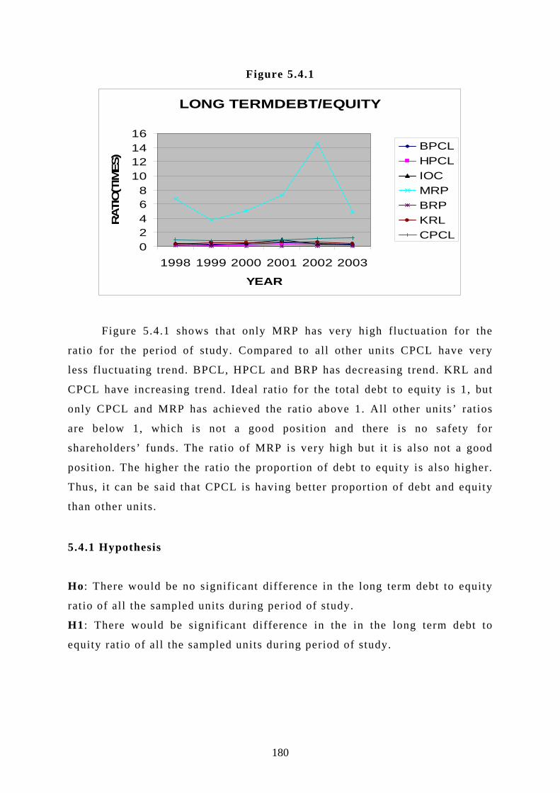
Figure 5.4.1
LONG TERMDEBT/EQUITY
02468
10121416
1998 1999 2000 2001 2002 2003
YEAR
RATI
O(T
IMES
)
BPCLHPCLIOCMRPBRPKRLCPCL
Figure 5.4.1 shows that only MRP has very high fluctuation for the
ratio for the period of study. Compared to all other units CPCL have very
less fluctuating trend. BPCL, HPCL and BRP has decreasing trend. KRL and
CPCL have increasing trend. Ideal ratio for the total debt to equity is 1, but
only CPCL and MRP has achieved the ratio above 1. All other units’ ratios
are below 1, which is not a good position and there is no safety for
shareholders’ funds. The ratio of MRP is very high but it is also not a good
position. The higher the ratio the proportion of debt to equity is also higher.
Thus, it can be said that CPCL is having better proportion of debt and equity
than other units.
5.4.1 Hypothesis
Ho: There would be no significant difference in the long term debt to equity
ratio of all the sampled units during period of study.
H1: There would be significant difference in the in the long term debt to
equity ratio of all the sampled units during period of study.
180

5.4.1(B) ANOVA Analysis
Source of
Variation
Sum of Squares
Degree of
Freedom (d.f .)
Mean Squares
F Value
Table Value
Between Samples 227.6 6 37.93 17.12 3.67
With in Samples 77.53 35 2.215
Total 305.1 41
Table 5.4.1(B) indicates the calculated value of ‘F’. The calculated
value of ‘F’ is 17.12 which are much higher than the table value of ‘F’. The
table value of ‘F’ at 5% levels of significance is 3.67. It indicates that the
null hypothesis is rejected and alternate hypothesis will remain. It indicates
that there is much significance difference in the long term debt to equity
ratio for the units undertaken for the study for the period of the study (i.e.
for six years). It means that proportion of keeping debt to its owned fund is
not same for all the units.
5.4.2 Total Debt to Equity Ratio
Total debt or external equities include all out side liabilities, both
short term and long term. In other words total, debt includes debentures,
sundry creditors, bills payable, bank overdraft, short and long term loans,
outstanding expenses, taxation, provision, proposed dividend etc. Equity
includes share capital (both equity and preference) and accumulated profits in
the form of general reserve, capital reserve and any other fund that belong to
the shareholder’s funds. The firm may be interested in knowing the
proportion of the interest bearing debt in capital structure. It may therefore
compute debt ratio by dividing total debt by equity( 7 ) .
181

Total debt equity ratio = Total debt (short term + long term) * 100
Equity
OR
Total debt equity ratio = External Equities * 100
Internal Equities
A low debt equity ratio implies a greater claim of owners than creditors
from the point of view of creditors. It represents a satisfactory situation since
a high proportion of equity provides a larger margin of safety for them.
The higher debt – equity ratio, the larger the shareholder’s earnings
when the cost of debt is less than the firm’s overall ratio of return on
investment. Thus there is need to strive a proper balance between the use of
debt and equity.
Table 5.4.2(A)
Total Debt to Equity Ratio Table YEAR REFINERIES
BPCL HPCL IOC MRP BRP KRL CPCL Overal l Trend
Mar-98 0.58 0.29 1.34 7.12 0.11 0.35 1 1.54
Mar-99 0.55 0.28 0.82 3.75 0.1 0.37 0.87 0.96
Mar-00 0.74 0.5 1.19 5.61 0.09 0.63 0.87 1.38
Mar-01 1.02 0.55 1.31 8.09 0.16 0.64 0.03 1.69
Mar-02 0.96 0.54 1.26 16.13 0.42 0.8 1.22 3.05
Mar-03 0.69 0.21 0.77 5.8 0.42 0.71 1.53 1.45
Average 0.76 0.40 1.12 7.75 0.22 0.58 0.92
(Source – annual reports of the company)
Table 5.4.2(A) indicates the total debt to equity ratio of sampled
refineries which indicates the relationship between total debts with equity.
The data is for six years. Table 5.2.2 this ra8tio shows mixed trends it was
0.58, 0.55, 0.74, 1.02, 0.96 and 0.69 for the respective year of 1998, 1999,
182

2000, 2001, 2002 and 2003. For HPCL it shows steady trends it was 0.29,
0.28, 0.5, 0.55, 0.54 and 0.21 for the respective years of 1998, 1999, 2000,
2001, 2002 and 2003. For IOC the ratio of sampled units shows decreasing
trends. The ratio ware 1.34, 0.82, 1.19, 1.31, 1.26 and 0.77 for the respective
years from 1998, 1999, 2000, 2001, 2002 and 2003. For MRP there was
significant fluctuation in the ratio. The trend was 7.12, 3.75, 5.61, 8.09,
16.13 and 5.8 for the respective years of 1998, 1999, 2000, 2001, 2002 and
2003. For BRP it shows steady trend. It was 0.11, 0.1, 0.09, 0.16, 0.42, and
0.42 for the year 1998, 1999, 2000, 2001, 2002 and 2003. For KRL it shows
increasing trend but there was very less fluctuations it was 0.35, 0.37, 0.63,
0.64, 0.8, and 0.71 for the year 1998, 1999, 2000, 2001, 2002 and 2003. For
CPCL it shows increasing trend but very slight fluctuations. It was 1, 0.87,
0.83, 0.03, 1.22, and 1.53 for the year 1998, 1999, 2000, 2001, 2002 and
2003. The average of the ratios of total debt to equity ratio of BPCL units is
0.76, HPCL is 0.40, IOC is 1.12, MRP is 7.75, BRP is 0.22, and KRL is 0.58
CPCL is 0.92. Further over all trend of the same ratio of all the units
undertaken for the study is for the year ending 1998 is 1.54, for the year
ending 1999 is 0.96, for the year ending 2000 is 1.38, for the year ending 2001 is
1.69, for the year ending 2002 is 3.05 and for the year ending 2003 is 1.45.
Figure 5.4.2
TOTAL DEBT / EQUITY
02468
1012141618
1998 1999 2000 2001 2002 2003
YEAR
RATI
O (T
IMES
)
BPCLHPCLIOCMRPBRPKRLCPCL
183

Figure 5.4.2 indicates that like long term debt to equity ratio, total debt
to equity ratio is also fluctuating in all the units for the period of the study.
But among them MRP has more fluctuations, while other units are having less
fluctuations. It shows that the amount of total debt in the year 1998 to 2003
fluctuates in all the units. The average of the ratio of MRP is highest and of
BRP is lowest. Only CPCL has achieved the ratio above 1 which is good
position for the firm. It shows that total debt is higher than the owner funds
so shareholders may have earnings on their investments. All other units have
the ratios below 1. so they have less debt than their owned funds.
Shareholders may not get the benefit of trading on equity.
5.4.2 Hypothesis
Ho: There would be no significant difference in the total debt to equity ratio
of all the sampled units during period of study.
H1: There would be significant difference in the in the total debt to equity
ratio of all the sampled units during period of study.
5.4.2(B) ANOVA Analysis
Source of Variation
Sum of Squares d.f Mean
F Value
Table Value
Between
Samples 261.5 6 43.59 15.68 3.67
With in Samples 97.31 35 2.78
Total 358.8 41
Table 5.4.2(B) indicates the calculated value of ‘F’. The calculated
value of ‘F’ is 15.68 which is much higher than the table value of ‘F’. The
table value of ‘F’ at 5% levels of significance is 3.67. It indicates that the
null hypothesis is rejected and alternate hypothesis will remain. It indicates
that there is much significant difference in the total debt to equity in the
units undertaken for the study for the research period of the study (i.e. for six
184

years). Thus it shows that liquidity position and earning of shareholders are
not same for the units for the given period.
5.4.3 Current Ratio
This ratio is most commonly used to perform the short term financial
analysis. It is also known as the working capital ratios. This ratio matches
the current assets to of the firm to the current l iabilit ies of the firm( 8 ) . This
ratio is an indication of the firm’s commitment to meet its short – term
liabilities. It is calculated by dividing current assets by current liabilities.
Current Ratio = Current Assets___
Current Liabilities
Current assets mean assets that will either be used up or converted into
cash within a year’s time or during normal operating cycle of business
whichever is higher. Current assets include cash and those assets which can
be converted into cash within a year such as marketable securities, debtors,
inventories, bills receivables, prepaid expenses( 9 ) .
Current liabilities include all obligations maturing within a year such
as sundry creditors, bills payable, and accrued expenses, short term bank
loan, income tax liabilities, and accrued taxes, long term debt maturing in
current year. Current liabilities mean liabilities payable within a year or
during the operating cycle whatever is longer out of the existing current
assets or by creation of current liabilities.
The current ratio is the measure of the firm’s short term solvency. It
indicates the availability of current assets in rupees for every one rupee of
current liabilities. A ratio of greater than one means that the firm has more
current assets than current claims against them( 1 0 ).
185

Normally a current ratio of 2:1 is considered satisfactory. In other
words current assets should be twice the amount of current l iabilit ies. If the
current ratio is 1:1, i t means that funds fielded by current assets are just
sufficient to pay the amounts due to various creditors and there will be
nothing left to meet the expenses which are being currently incurred. Thus
the ratio should always be more than 1:1. A very high current ratio is also not
desirable because it indicates idleness of funds which is not a sign of
efficient financial management( 1 1 ). This is because a high current ratio means
excessive depended on long term sources of rising funds long- term liabilities
are customer than current liabilities and therefore, this will result in
considerably lowering down the profitability of the concern.
Thus, the current ratio is an index of the concern’s financial stability
since it shows the extent of the working capital which is the amount by which
the current assets exceed the current liabilities. As stated earlier a higher
current ratio would indicate inadequate employment of funds while a poor
current ratio is a danger signal to the management. It shows that business is
trading beyond its resources.
Table 5.4.3(A)
Current Ratio Table YEAR REFINERIES
BPCL HPCL IOC MRP BRP KRL CPCL Overall Trend
Mar-98 0.81 0.78 0.83 0.94 1.58 1.16 1.163 1.04
Mar-99 0.89 1.01 0.8 2.75 1.79 1.14 1.153 1.36
Mar-00 0.91 1.03 1.05 1.44 1.58 1.14 1.97 1.30
Mar-01 0.92 1.25 1.34 0.7 1.26 1.22 2.364 1.29
Mar-02 0.76 1.51 0.75 0.71 0.55 1.66 1.934 1.12
Mar-03 0.89 1.2 0.95 0.78 0.96 1.48 1.302 1.08
Average 0.86 1.13 0.95 1.22 1.29 1.30 1.65
(Source – annual reports of the company)
Table 5.4.3(A) indicates the ratio of current assets to current liabilities
of the sampled units for the period undertaken for the study. It indicates the
186

relationship between current assets to current liabilities. The data was for six
years. For BPCL this ratio shows steady trends it was 0.81 , 0.89, 0.91, 0.92,
0.76 and 0.89 for the respective year of 1998, 1999, 2000, 2001, 2002 and
2003. For HPCL it was 0.78, 1.01, 1.03, 1.25, 1.51 and 1.2 for the respective
years of 1998, 1999, 2000, 2001, 2002 and 2003. This ratio of HPCL shows
very less increasing trends. For IOC the ratio of sampled units shows mixed
trends. The ratio ware 0.83, 0.8, 1.05, 1.34, 0.75 and 0.95 for the respective
years from 1998, 1999, 2000, 2001, 2002 and 2003. For MRP the ratio were
0.94, 2.75, 1.44, 0.07, 0.71 and 0.78 for the respective years of 1998, 1999,
2000, 2001, 2002 and 2003. It shows decreasing trends. For BRP ratio was
1.58, 1.79, 1.58, 1.26, 0.55, and 0.96 for the year 1998, 1999, 2000, 2001,
2002 and 2003. It shows decreasing trends. For KRL ratio was 1.16, 1.14,
1.14, 1.22, 1.66, and 1.48 for the year 1998, 1999, 2000, 2001, 2002 and
2003.It shows very less increasing trends. For CPCL ratio was 1.163, 1.153,
1.97, 2.264, 1.934, and 1.302 for the year 1998, 1999, 2000, 2001, 2002 and
2003. It shows mixed trends. There was high rise in the year 2001 but after
that it decreases. The average of current ratios of BPCL units is 0.86, HPCL
is 1.13, IOC is 0.95, MRP is 1.22, BRP is 1.29, KRL is 1.30, and CPCL is
1.65. Further over all trend of the same ratio of all the units undertaken for
the study is for the year ending 1998 is 1.04, for the year ending 1999 is
1.36, for the year ending 2000 is 1.30, for the year ending 2001 is 1.29, for
the year ending 2002 is 1.12 and for the year ending 2003 is 1.08.
Figure 5.4.3
Current Ratio
0
0.5
1
1.5
2
2.5
3
1998 1999 2000 2001 2002 2003
Year
Ratio
BPCLHPCLIOCMRPBRPKRLCPCL
187

Seeing to figure 5.4.3 it can be seen that all the units are having mixed
trend however liquidity has decreased in CPCL, BRP, MRP in the year 2003
compared to 1993. BPCL has least average compared to other units. Only
KRL, CPCL and HPCL have maintained the ratio of 1:1 means they have
more current assets than current liabilities through out the research period,
however it is not the ideal ratio 2:1. Further, overall trend of the ratio for the
period 1998 to 2003 have less fluctuations and it is above 1:1.
5.4.3 Hypothesis
Ho: There would be no significant difference in the current ratio
of all the sampled units during period of study.
H1: There would be significant difference in the in the current ratio of
all the sampled units during period of study.
5.4.3(B) ANOVA Analysis
Source of
Variation
Sum of Squares
Degree of Freedom (d.f .)
Mean Squares
F Value
Table Value
Between Samples 2.370 6 0.3950 2.169 3.67
With in Samples 6.374 35 0.1821
Total 8.744 41
Table 5.4.3(B) table indicates the calculated value of ‘F’. The
calculated value of ‘F’ is 2.169 which is less than the table value. The table
value of ‘F’ at 5% levels of significance is 3.67. It indicates that the null
hypothesis is accepted and alternate hypothesis will rejected. It indicates that
there is no significant difference of maintaining the proportion of current
assets and current liabilities between the units undertaken for the study for
the period of the study (i.e. for six years).
188

5.4.4 Interest Coverage Ratio
These ratios indicate the extent to which the interest of the persons
entitled to get a fixed return as per the agreed terms is safe. The higher the
cover better i t is. This is very important from the lender’s point of view
because it indicates the ability of a company to pay interest out of its profits.
It indicates whether the business would earn sufficient profits to pay
periodically the interest charges(12 ). This ratio is determined by dividing
earning before interest and taxes by the interest charges.
Interest Coverage Ratio = EBIT (Earning Before Interest and Taxes)
Interest
This ratio shows the number of times the interest charges are covered
by the funds that are ordinarily available for their payment. Since taxes are
computed after interest. Interest coverage is calculated in relation to before
tax earnings depreciation is non-cash item. Therefore funds equal to
depreciation are also available to pay interest charges. The standard for this
ratio for an industrial company is that interest charges should be covered six
to seven times( 1 3 ).
This ratio measures the extent to which operating income can decline
before the firm is unable to meet its annual interest cost. Failure to meet
these obligations can bring legal action by the firm’s creditors possibly
resulting in bankruptcy. Earning before interest and taxes, rather than net
income, is used in the numerator because interest is paid with pre – tax
rupees, the firm’s abili ty to pay current interest is not affected by taxes( 1 4 ).
189

Table 5.4.4(A)
Interest Cover (Time) YEAR REFINERIES
BPCL HPCL IOC MRP BRP KRL CPCL Overall Trend
Mar-98 7.4 10.83 2.38 1.07 5.04 8.13 1.91 5.25
Mar-99 6.45 11.08 3.64 0.98 4.23 10.87 3.41 5.81
Mar-00 6.08 9.44 3.9 0 4.5 8.18 3.19 5.04
Mar-01 5.19 4.27 2.61 -0.5 -4.36 1.86 1.92 1.57
Mar-02 5.56 5.18 4.07 -0.2 -7.11 2.04 1.65 1.60
Mar-03 9 16.68 11.23 -0.02 12.49 8.34 5.52 9.03
Average 6.61 9.58 4.64 0.22 2.47 6.57 2.93
(Source – annual reports of the company)
Table 5.4.4(A) indicates the ratio of interest coverage of the sampled
units for the period undertaken for the study. It indicates the relationship
between EBIT (earning before interest and tax) and interest to be paid. The
data was for six years. For BPCL this ratio shows decreasing trend except in
the year 2003. It was 7.4 , 6.45, 6.08, 5.19, 5.56 and 9 for the respective year
of 1998, 1999, 2000, 2001, 2002 and 2003. For HPCL it was 10.83, 11.08,
9.44, 4.25, 5.18 and 16.68 for the respective years of 1998, 1999, 2000, 2001,
2002 and 2003. These ratios of HPCL shows decreasing trend except in the
year 2003. For IOC the ratio of sampled units shows mixed trend but there
was high rise in the year 2003. The ratio ware 2.38, 3.68, 3.9, 2.61, 4.07 and
11.23 for the respective years from 1998, 1999, 2000, 2001, 2002 and 2003.
For MRP the ratio were 1.07, 0.98, 0, -0.5, -0.2 and -0.02 for the respective
years of 1998, 1999, 2000, 2001, 2002 and 2003. It shows decreasing trend.
For BRP ratio was 5.04, 4.23, 4.5, -4.36, -7.11, and 12.49 for the year 1998,
1999, 2000, 2001, 2002 and 2003. It shows mixed trend. For KRL ratio was
8.13, 10.87, 8.18, 1.86, 2.04, and 8.34 for the year 1998, 1999, 2000, 2001,
2002 and 2003.It shows mixed trend. For CPCL it has also mixed trend. It
was 1.91, 3.41, 3.19, 1.92, 1.65, and 5.52 for the year 1998, 1999, 2000,
2001, 2002 and 2003.Generally all the sampled units have mixed trends. The
average of the ratios of interest coverage of BPCL units is 6.61, HPCL is
9.58, IOC is 4.64, MRP is 0.22, BRP is 2.47, KRL is 6.57 and CPCL is 2.93.
190

Further over all trend of the same ratio of all the units undertaken for the
study is for the year ending 1998 is 5.25, for the year ending 1999 is 5.81,
for the year ending 2000 is 5.04, for the year ending 2001 is 1.57, for the
year ending 2002 is 1.60 and for the year ending 2003 is 9.03.
Figure 5.4.4
INTEREST COVER (TIME)
-10
0
10
20
1998 1999 2000 2001 2002 2003
YEAR
RATI
O
BPCLHPCLIOCMRPBRPKRLCPCL
F igure 5.5 shows that HPCL has the highest interest coverage in the
year 2003 than other unit, but it is fluctuating every year. BPCL has good
average and also less fluctuation during the period of study. IOC and BRP
has increased their interest coverage in the year 2003 compared to 1998.
MRP and BRP unit have not cover the interest even once in many years as
they have less than one ratio. It means they have not enough earning to cover
interest particularly in those years. IOC ratio has increased much so that i t
can be said that its earnings may be higher to cover the interest. Overall
industry has poor interest coverage in the year 2001 and 2002 because of poor
performance of MRP and BRP. But it increased in 2003 because except MRP all the
units have good performance. Overall IOC’s performance is good.
5.4.4 Hypothesis
Ho: There would be no significant difference in the interest coverage ratio
of all the sampled units during period of study.
191

H1: There would be significant difference in the in the interest coverage ratio
of all the sampled units during period of study.
5.4.4(B) ANOVA Analysis
Source of
Variation
Sum of
Squares
Degree of
Freedom (d.f .)
Mean Squares
F Value
Table Value
Between Samples 354.9 6 59.15 4.133 3.67
With in Samples 500.9 35 14.31
Total 855.8 41
Table 5.4.5(B) table indicates the calculated value of ‘F’. The
calculated value of ‘F’ is 4.133 which is higher than the table value of ‘F’.
The table value of ‘F’ at 5% levels of significance is 3.67. It indicates that
the null hypothesis is rejected and alternate hypothesis will remain. It
indicates that there is a significant difference for the interest coverage ratio
between the units undertaken for the study for the period of the study (i .e. for
six years). Thus it can be said that earnings before interest and taxes related
to interest charges are not same for the sampled units for the research period.
5.4.5 Gross Working Capital Cycle (Days)
This is also known as gross working capital leverage Ratio. This ratio
indicates whether or not working capital has not been effectively utilized in
making sales.
Gross Working Capital Cycle Ratio (days) = Sales * 365
Gross Working capital
In case a company can achieve higher volume of sales with relatively small
amount of working capital. It is an indication of the operating efficiency of the
192

company. If a sale is more than working capital it will be utilized for less days and
vice – a- versa if sales is less, gross working capital will be utilized for more days.
Table 5.4.5(A)
Gross Working Capital Cycle (Days) YEAR REFINERIES
BPCL HPCL IOC MRP BRP KRL CPCL Overall Trend
Mar-98 71 120 70 106 95 37 115 88
Mar-99 46 57 69 38 97 43 67 60
Mar-00 48 62 79 57 76 46 64 62
Mar-01 47 55 77 108 91 44 62 70
Mar-02 57 60 82 75 86 54 68 69
Mar-03 48 56 81 58 73 53 88 65
Average 53 68 76 73 86 46 77
(Source – annual reports of the company)
Table 5.4.5(A) indicates the ratio of Gross Working Capital Cycle of
the sampled units for the period undertaken for the study. The data was for
six years. It indicates how many times Gross working capital has been
utilized in relation with sales. For BPCL this ratio shows decreasing trend. It
was 71 , 46, 48, 47, 57 and 48 for the respective year of 1998, 1999, 2000,
2001, 2002 and 2003. For HPCL it was 120, 57, 62, 55, 60 and 56 for the
respective years of 1998, 1999, 2000, 2001, 2002 and 2003. This shows that
the ratio of HPCL shows decreasing trend. For IOC the ratio of sampled units
shows mixed trend. The ratio ware 70, 69, 79, 77, 82 and 81 for the
respective years from 1998, 1999, 2000, 2001, 2002 and 2003. For MRP the
ratio were 106, 38, 57, 108, 75 and 58 for the respective years of 1998, 1999,
2000, 2001, 2002 and 2003. It shows mixed trend and has vary high
fluctuation. For BRP ratio was 95, 97, 76, 91, 86, and 73 for the year 1998,
1999, 2000, 2001, 2002 and 2003. It shows mixed trend. For KRL ratio were
37, 43, 46, 44, 54, and 53 for the year 1998, 1999, 2000, 2001, 2002 and
2003.It shows increasing trend. For CPCL it has also decreasing trend. It was
115, 67, 64, 62, 68, and 88 for the year 1998, 1999, 2000, 2001, 2002 and
193

2003. The average of gross working capital cycle of BPCL units is 53, HPCL
is 68, IOC is 76, MRP is 74, BRP is 86, KRL is 46 and CPCL is 77. Further
over all trend of the same ratio of all the units undertaken for the study is for
the year ending 1998 is 88, for the year ending 1999 is 60, for the year
ending 2000 is 62, for the year ending 2001 is 69, for the year ending 2002 is
67 and for the year ending 2003 is 65.
Figure 5.4.5
GROSS WORKING CAPITAL CYCLE (DAYS)
0
20
40
60
80
100
120
140
1998 1999 2000 2001 2002 2003
YEARS
RATI
O
BPCLHPCLIOCMRPBRPKRLCPCL
Table 5.4.5 shows that IOC has maintained their working capital cycle.
KRL has also improved its efficiency in using working capital. But all other
units have decreased their ratio it means they have not maintained their
efficiency in using working capital during the period of study. HPCL have
decreased a lot in the ratio, i t means its working capital is used for more days
and its sales may be decreasing. MRP has more fluctuations so it can be said
that sales may be not steady.
5.4.5 Hypothesis
Ho: There would be no significant difference in the ratio of gross working
capital cycle of all the sampled units during period of study.
194

H1: There would be significant difference in the in the ratio of Gross
working capital cycles of all the sampled units during period of study.
5.4.5(B) ANOVA Analysis
Source of
Variation
Sum of Squares
Degree of
Freedom (d.f .)
Mean Squares
F Value
Table Value
Between Samples 7368 6 1228 4.006 3.67
With in Samples 1.0730E+04 35 306.6
Total 1.8099E+04 41
Table 5.4.5(B) indicates the calculation calculated value of ‘F’. The
calculated value of ‘F’ is 4.006 which is higher than the table value of ‘F’.
The table value of ‘F at 5% levels of significance is 3.67. It indicates that the
null hypothesis is rejected and alternate hypothesis will remain. It indicates
that there is significant difference in the gross working capital cycle of the
sampled units undertaken for the study for the period of the study (i.e. for six
years). So it can be said that ratio of sales to working capital with relation to
365 days differs in all the units for the research period.
5.4.6 Net Working capital cycle (days)
The difference between current assets and current liabilities excluding
short term borrowings is called net working capital (NWC) or net current
assets (NCA). Net Working Capital is sometimes used as measure of a
firm’s liquidity. It is considered that between two firms the one having larger
NWC has the greater ability to meet its current obligations(15 ).
Net Working Capital Cycle Ratio (Days) = __ Sales * 365
Net Working Cycle
195

A high net working capital turnover ratio shows the efficient
utilization of working capital in generating sales. A low ratio, on the other
hand, may indicate the excess of net working capital. This ratio thus shows
weather working capital is efficiently used or not. This ratio is considered
better than stock turnover ratio because it shows the utilization of the entire
working capital when as the stock turnover ratio indicates only the turnover
of inventories which is only a part of the working capital.
Table 5.4.6(A)
Net Working Capital Cycle (Days)
REFINERIES YEAR BPCL HPCL IOC MRP BRP KRL CPCL Overal l Trend
Mar-98 49 108 27 36 57 0 -116 23 Mar-99 35 45 34 9 61 1 -126 8 Mar-00 35 51 47 22 45 9 -28 26 Mar-01 38 49 51 17 73 12 34 39 Mar-02 46 55 53 -3 50 17 35 36 Mar-03 26 51 52 9 30 23 31 32 Average 38 60 44 15 53 10 -28 (Source – annual reports of the company)
Table 5.4.6(A) indicates the ratio of Net Working Capital Cycle of the
sampled units for the period undertaken for the study. The data was for six
years. It indicates how many times Net working capital has been utilized in
relation with sales. For BPCL this ratio shows mixed trend. It was 49 , 35, 35,
38, 46 and 26 for the respective year of 1998, 1999, 2000, 2001, 2002 and
2003. For HPCL it was 108, 45, 51, 49, 55 and 51 for the respective years of
1998, 1999, 2000, 2001, 2002 and 2003. This ratio of HPCL shows mixed
trend and there is high fluctuation in the ratios. For IOC the ratio of sampled
units shows increasing trend. The ratio ware 27, 34, 47, 51, 53 and 52 for the
respective years from 1998, 1999, 2000, 2001, 2002 and 2003. For MRP the
ratio were 36, 9, 22, 70, -3 and 9 for the respective years of 1998, 1999,
2000, 2001, 2002 and 2003. It shows decreasing trend. For BRP ratio was 57,
61, 45, 73, 50, and 30 for the year 1998, 1999, 2000, 2001, 2002 and 2003. It
shows mixed trend. For KRL ratio ware 0, 1, 9, 12, 17, and 23 for the year
1998, 1999, 2000, 2001, 2002 and 2003.It shows increasing trend. For CPCL
196

i t has also high fluctuation trend. It was -116, -126, -28, 34, 35, and 31 for
the year 1998, 1999, 2000, 2001, 2002 and 2003. The average of net working
capital cycle of BPCL units is 38, HPCL is 60, IOC is 44, MRP is 15, BRP is
53, KRL is 10 and CPCL is -28. Further over all trend of the same ratio of all
the units undertaken for the study is for the year ending 1998 is 23, for the
year ending 1999 is 8, for the year ending 2000 is 26, for the year ending
2001 is 40, for the year ending 2002 is 36 and for the year ending 2003 is 32.
Figure 5.4.6
NET WORKING CAPITAL (DAYS)
-150
-100
-50
0
50
100
150
1998 1999 2000 2001 2002 2003
YEARS
RATI
O
BPCLHPCLIOCMRPBRPKRLCPCL
The table 5.4.6 indicates that BPCL and HPCL liquidity position is decreased
during the period of study. MRP has very high fluctuation in their working capital
utilization efficiency. Only IOC has improved its cycle so it has better position. So
it can be said that IOC has used their working capital very efficiently. The
utilization of working capital of CPCL was very poor in early years but slowly it has
improved. KRL has also improved a lot in efficient use of working capital.
5.4.6 Hypothesis
Ho: There would be no significant difference in the ratio of net working
capital cycle of all the sampled units during period of study.
197

H1: There would be significant difference in the in the ratio of net working
capital cycles of all the sampled units during period of study.
5.4.6(B) ANOVA Analysis
Source of
Variation
Sum of Squares
Degree of
Freedom (d.f .)
Mean Squares
F Value
Table Value
Between Samples 3.3798E+04 6 5633. 5.667 3.67
With in Samples 3.4792E+04 35 994.0
Total 6.8590E+04 41
Table 5.4.6(B) indicates the calculated value of ‘F’. The calculated
value of ‘F’ is 5.67. The calculated value is much higher than the table value.
The table value of ‘F’ at 5% levels of significance is 3.67. It indicates that
the null hypothesis is rejected and alternate hypothesis will remain. It
indicates that there are significant different in the net working capital
cycle(days) of the sampled units undertaken for the study for the period of
the study (i.e. for six years). Calculated value of ‘F’ is not much higher than
table value of ‘F’. so it can be said that there is very little significant
difference between the units for the utilization of working capital. However
all the units have different efficiency in the utilization of working capital. .
5.4.7 Average days of Debtors
A firm sells goods for cash and credit is used as a marketing tool by a
number of companies which the firm extends credits to its customers book
debts. Debtors or receivables are created in the firm’s accounts. Book debts
are expected is to be converted into cash over a short period and therefore,
are included in current assets. The liquidity position of the firm depends on
the quality of debtors to a great extent. Financial analysts apply debtor
turnover ratio and average collection period to judge quality or liquidity of
198

debtors( 1 6 ) . Debtors turn over, collection period, again Schedule of debtors.
The term debtors include trade debtors and bills receivables. Doubtful debts
are not deducted from debtors. The debtor turnover ratio indicates the
relationship between net credit sales and average days of debtors( 1 7 ) . The
debtors’ turnover ratio is usually supplemented by average collection period
(Average days of debtors). It can be calculated as follows:
Average Days of Debtors = Average Debtors * 365
Sales
The significance of this ratio lies in the fact that debtors constitute one
of the important items of current assets and this ratio indicates as to how
many days average sales are tied up in the amount of debtors. Changes in this
ratio show the changes in the company’s credit policy.
Table 5.4.7(A)
Average Days of Debtors YEAR REFINERIES
BPCL HPCL IOC MRP BRP KRL CPCL Overal l Trend
Mar-98 9 5 14 4 6 1 6 6
Mar-99 9 5 12 5 7 2 6 7
Mar-00 8 5 13 8 7 4 9 8
Mar-01 7 4 13 16 6 3 11 9
Mar-02 8 5 13 21 6 13 1 10
Mar-03 6 5 11 16 14 23 20 14
Average 8 5 13 12 8 8 9
(Source – annual reports of the company)
Table 5.4.7(A) indicates the Average Days of Debtors of the sampled
units for the period undertaken for the study. The data was for six years. It
shows that the average collection period for the credit sales. For BPCL this
ratio shows decreasing trend. It was 9 , 9, 8, 7, 8 and 6 for the respective year
of 1998, 1999, 2000, 2001, 2002 and 2003. For HPCL it was 5, 5, 5, 4, 5 and
5 for the respective years of 1998, 1999, 2000, 2001, 2002 and 2003. This
199

ratio of HPCL shows steady trend. For IOC the ratio of sampled units shows
mixed trend. The ratio ware 14, 12, 13, 13, 15 and 11 for the respective years
from 1998, 1999, 2000, 2001, 2002 and 2003. It has high fluctuation and has
mixed trend. For MRP the ratio were 14, 12, 13, 13, 13 and 11 for the
respective years of 1998, 1999, 2000, 2001, 2002 and 2003. It has mixed
trend. For BRP ratio was 6, 7, 7, 6, 6, and 14 for the year 1998, 1999, 2000,
2001, 2002 and 2003. It shows mixed trend. For KRL ratio ware 1, 2, 4, 3,
13, and 23 for the year 1998, 1999, 2000, 2001, 2002 and 2003.It shows
mixed trend. For CPCL it has mixed trend. It was 6, 6, 9, 11, 1, and 20 for
the year 1998, 1999, 2000, 2001, 2002 and 2003. The average of average days
of debtors of BPCL units is 8, HPCL is 5, IOC is 13, MRP is 12, BRP is 8,
KRL is 8 and CPCL is 9. Further over all trend of the same ratio of all the
units undertaken for the study is for the year ending 1998 is 6, for the year
ending 1999 is 6, for the year ending 2000 is 8, for the year ending 2001 is 8,
for the year ending 2002 is 10 and for the year ending 2003 is 14.
Figure 5.4.7
AVG DAYS DEBTORS
0
5
10
15
20
25
1998 1999 2000 2001 2002 2003
YEAR
RATI
O (T
IMES
)
BPCLHPCLIOCMRPBRPKRLCPCL
Table 5.4.7 shows that average days of debtors posit ion is good in
MRP, BRP, CPCL, KRL. It indicates that all these units have increased their
collection period so their sales tied up in the debtors for less days. While in
200

IOC and BPCL the days of average of debtors decreased. They take long time
to collect their debts from debtors. HPCL is steady in its policy of collection
of debts from debtors.
5.4.7 Hypothesis
Ho: There would be no significant difference in the ratio of average days of
debtors of all the sampled units during period of study.
H1: There would be significant difference in the in the ratio of average days
of debtors of all the sampled units during period of study.
5.4.7(B) ANOVA Analysis
Source of
Variation
Sum of Squares
Degree of Freedom (d.f .)
Mean Squares
F Value
Table Value
Between Samples 254.3 6 42.38 1.675 3.67
With in Samples 885.8 35 25.31
Total 1140 41
Table 5.4.7(B) indicates the calculated value of ‘F’. The calculated
value of ‘F’ is 1.675 which is much lower than the table value of ‘F’. The
table value of ‘F’ at 5% levels of significance is 3.67. This is less than the
calculated value of ‘F’. It indicates that the null hypothesis is accepted and
alternate hypothesis will rejected. It indicates that there are no significant
different in the average days of debtors of the sampled units undertaken for
the study for the period of the study (i.e. for six years). It indicates that all
the units have almost same period to collect their debts, so their liquidity
position is almost remains same.
201

5.4.8 Average Days of Creditors
It is similar to debtor’s turnover ratio. It indicates the speed with
which the payments for credit purchase are made to the creditors. The ratio
can compute as follows:
Average Days of Creditors = Average Creditors * 365
Purchases
The term creditors mean “Trade Creditors” and “Bill Payable”. In case
the detail regarding credit purchases, opening and closing accounts payable
have not been given to decide average creditors, the ratio may be calculated
by talking total purchases to compute average creditors. The ratio gives
average credit period enjoyed from the creditors. Both the creditors turnover
ratio and the debt payment period enjoyed the ratio indicate about the
promptness or otherwise in marketing payment of credit purchases. A lower
credit period ratio signifies that the creditors are being paid promptly, thus
enhancing the creditworthiness of the company. However a very favorable
ratio to this effect also shows that the business is not taking the full
advantage of credit facilities which can be allowed by the creditors(1 8 ) . Thus,
in general the longer the credit period achieved the better because delays in
payment mean the operation of the company are being financed interest free
by suppliers of funds. But there will be a point beyond which if they are
operating in a seller’s market may harm the company. If too long a period
taken to pay creditors the credit rating of the company may suffer, thereby
making it more difficult to obtain supplies in future( 1 9 ).
202

Table 5.4.8(A)
Average Days of Creditors YEAR REFINERIES
BPCL HPCL IOC MRP BRP KRL CPCL Overal l Trend
Mar-98 22 12 43 70 38 38 231 65
Mar-99 10 12 34 29 35 41 193 51
Mar-00 12 11 32 34 30 37 93 36
Mar-01 9 6 26 91 18 31 27 30
Mar-02 11 4 29 78 35 36 32 32
Mar-03 21 4 29 49 60 29 35 32
Average 14 8 32 59 36 35 102
(Source – annual reports of the company)
Table 5.4.8(A) indicates the ratio of Average days Creditors of the
sampled units for the period undertaken for the study. The data was for six
years. It indicates the average credit period for the credit purchases. For
BPCL this ratio shows mixed trend. It was 22 , 10, 12, 9, 11 and 21 for the
respective year of 1998, 1999, 2000, 2001, 2002 and 2003. For HPCL it was
12, 12, 11, 6, 4 and 4 for the respective years of 1998, 1999, 2000, 2001,
2002 and 2003. It shows that ratios of HPCL show decreasing trend. For IOC
it shows decreasing trend. The ratio ware 43, 54, 32, 26, 29 and 21 for the
respective years from 1998, 1999, 2000, 2001, 2002 and 2003. For MRP the
ratio were 70, 29, 34, 91, 78 and 49 for the respective years of 1998, 1999,
2000, 2001, 2002 and 2003. It shows mixed trend and has vary high
fluctuation. For BRP ratio was 38, 45, 13, 18, 35, and 60 for the year 1998,
1999, 2000, 2001, 2002 and 2003. It shows mixed trend. For KRL ratio ware
38, 41, 57, 31, 36, and 29 for the year 1998, 1999, 2000, 2001, 2002 and
2003.It shows mixed trend. For CPCL it has high fluctuation and mixed
trend. It was 231, 193, 93, 27, 32, and 35 for the year 1998, 1999, 2000,
2001, 2002 and 2003. Thus except HPCL there are mixed trend for all
sampled units. For CPCL average days of creditors were decreasing very fast
year by year and again it rises. The average of average days of creditors of
BPCL units is 14, HPCL is 8, IOC is 32, MRP is 59, BRP is 36, KRL is 35
and CPCL is 102. Further over all trend of the same ratio of all the units
203

undertaken for the study is for the year ending 1998 is 65, for the year ending
1999 is 51, for the year ending 2000 is 36, for the year ending 2001 is 30, for
the year ending 2002 is 32 and for the year ending 2003 is 32.
Figure 5.4.8
AVG DAYS CREDITORS
0
50
100
150
200
250
1998 1999 2000 2001 2002 2003
YEAR
RATI
O (T
IMES
)
BPCLHPCLIOCMRPBRPKRLCPCL
Table 5.4.8 shows that HPCL is paying promptly to its creditors. While
BRP is taking a long period to pay to its creditors which may harm the
company to get credit in future. CPCL was taking a long period for payment
to creditors but i t has improved a lot in his credit policy and its payment days
has decreased to 35 only which is good period for credit payments. Thus,
CPCL has improved its policy of payment to creditors. KRL, MRP, IOC have
also decreased their credit payment period. Thus most of the units have good
credit policy. BPCL has fluctuations in the credit payment policy for the
research period.
5.4.8 Hypothesis
Ho: There would be no significant difference in the ratio of average days of
creditors of all the sampled units during period of study.
H1: There would be significant difference in the in the ratio of average days
of creditors of all the sampled units during period of study.
204

5.4.8(B) ANOVA Analysis
Source of
Variation
Sum of Squares
Degree of
Freedom (d.f .)
Mean Squares
F Value
Table Value
Between 3.5640E+04 6 5940. 4.660 3.67
With in Samples 4.4612E+04 35 1275.
Total 8.0252E+04 41
Table 5.4.8(B) indicates the calculated value of ‘F’. The calculated
value of ‘F’ is 4.660. The table value of ‘F’ at 5% levels of significance is
3.67. This is lower than the calculated value of ‘F’. It indicates that the null
hypothesis is rejected and alternate hypothesis will remain. It indicates that
there are significant differences in the average days of creditors of the
sampled units undertaken for the study for the period of the study (i.e. for six
years). It indicates that units differ in their credit payment policy. There is
no same period for credit payments given by the creditors against the
purchases of goods etc.
5.5 Inventory Management
Inventories constitute the most significant part of current assets of a
large majority of companies in India. On an average, inventories are
approximately 60 per cent of current assets in public limited companies in
India. Because of the large size of inventories maintained by firms, a
considerable amount of funds is required to be committed to them. It is
therefore, absolutely imperative to mange inventories efficiently and
effectively in order to avoid unnecessary investment. An undertaking
neglecting the management of inventories will be jeopardizing its long run
profitability and may fail ultimately. It is possible for a company to reduce
its levels of inventories to a considerable degree, e.g., 10 to 20 per cent,
without any adverse effect on production and sales, by using simple
inventory planning and control techniques. The reduction in “excessive”
205

inventories carries a favorable impact on a company’s profitability. In the
manufacturing firm’s inventory consist of three components.
1. Raw Materials
Raw materials are those basic inputs that are converted into finished
product through the manufacturing process. Raw materials inventories are
those units which have been purchased and stored for future productions.
2. Work – In – Process
Work – In – Process inventories are semi manufactured products. They
represent products that need more work before they become finished products
for sale.
3. Finished Goods
Finished Goods are those completely manufactured products which are
ready for sale. Stocks of raw materials and work in process facilitate
production while stock of finished goods is required for smooth marketing
operations. Thus, inventories serve as a link between the production and
consumption of goods.
A level of three kinds of inventories for a firm depends on the nature
of its business. A manufacturing firm which have substantially high levels of
all three kinds of inventories, while a retail or wholesale firm will have a
very high level of finished goods inventories and no raw materials and work
in process inventories. Within manufacturing firms there will be difference.
Large heavy engineering companies produce long production cycle products;
therefore, they carry large inventories. On the other hand, inventories of a
consumer product company will not be large because of short production
cycle and fast turnover.
206

A fourth kind of inventory supplies are also maintained by firm.
Supplies include office and plant cleaning materials, oil, l ight bulbs and the
like. These materials don not directly enter production but are necessary for
production process. Usually, these supplies are small parts of the total
inventory and do not involve significant investment. Therefore, a
sophisticated system of inventory control may not be maintained for them.
An analyst may also be interested in examining the efficiency with
which the firm converts raw materials into work in process and work in
process into finished goods. That is he would like to know the levels of raw
material inventory and work in process inventory and work in process
inventory had by the firm on an average. The raw material inventory should
be related to materials consumed and work in process to the cost of
production.
The inventory turnover shows how rapidly the inventory’s turning into
receivable through sales. Generally a high inventory turnover is indicative of
good inventory management. A low inventory turnover implies excessive
inventory levels than warranted by production and sales activities or a slow-
moving or obsolete inventory. A high level of sluggish inventory amounts to
unnecessary lie-up of funds reduced profit and increased costs. If the
obsolete inventories have to be written off this will adversely offset the
working capital and liquidity position of the firm. Again a relatively high
inventory turnover should be carefully analysed. A high inventory turnover
may be the result of a very low level of inventory which results in frequent
stakeouts, the firm may be living from hand to much. Thus too high and low
inventory turnover ratios should be investigated further. There are two
inventory turnover ratios have analysed. One is finished goods turnover
ratios and second one is raw material turnover ratio.
207

5.5.1 Finished Goods Turnover Ratio (Times)
Table 5.5.1(A)
Finished Goods Turnover Ratio (Times) Table
REFINERIES YEAR BPCL HPCL IOC MRP BRP KRL CPCL Overall Trend
Mar-98 16.28 31.88 19.44 30.54 7.6 111.91 15.79 33.35 Mar-99 25.99 27.82 19.46 46.01 8.23 73.76 22.57 31.98 Mar-00 14.35 13.09 15.19 15.8 10.34 57.93 25.78 21.78 Mar-01 14.34 14.13 16.18 7.67 10 58.86 38.56 22.82 Mar-02 12.38 13.89 15.56 13.73 15.23 34.94 32.92 19.81 Mar-03 12.64 14.55 14.5 21.55 17.66 32.52 23.29 19.53
Average 16.00 19.23 16.72 22.55 11.51 61.65 26.49 (Source – annual reports of the company)
Table 5.5.1(A) indicates the ratio of Finished Goods Turnover Ratio
(Times) of the sampled units for the period undertaken for the study. The
data was for six years. It indicates the average credit period for the credit
purchases. For BPCL this ratio shows decreasing trend. It was 16.28, 25.99,
14.35, 14.34, 12.38 and 12.64 for the respective year of 1998, 1999, 2000,
2001, 2002 and 2003. For HPCL it was 31.88, 27.82, 13.09, 14.13, 13.89 and
14.55 for the respective years of 1998, 1999, 2000, 2001, 2002 and 2003. It
shows that the ratios of HPCL shows decreasing trend. For IOC it shows
decreasing trend. The ratio ware 19.44, 19.46, 15.19, 16.18, 15.56 and 14.50
for the respective years from 1998, 1999, 2000, 2001, 2002 and 2003. It is
also having decreasing trend. For MRP the ratio were 30.54, 46.01, 15.80,
7.67, 13.73 and 21.55 for the respective years of 1998, 1999, 2000, 2001,
2002 and 2003. It shows mixed trend. For BRP ratio was 7.60, 8.23, 10.34,
10.00, 15.23, and 17.66 for the year 1998, 1999, 2000, 2001, 2002 and 2003.
It shows increasing trend. For KRL ratio ware 111.91, 73.76, 57.93, 58.86,
34.94, and 32.52 for the year 1998, 1999, 2000, 2001, 2002 and 2003.It
shows decreasing trend. For CPCL it has increasing trend. It was 15.79,
22.57, 25.78, 38.56, 32.92, and 23.29 for the year 1998, 1999, 2000, 2001,
2002 and 2003. Thus except BRP and CPCL there are decreasing trend for all
sampled units. The average of Finished Goods Turnover Ratio (Times) of
208

BPCL units is 16, HPCL is 19.23, IOC is 16.72, MRP is 22.55, BRP is 11.51,
KRL is 61.65 and CPCL is 26.49. Further over all trend of the same ratio of
all the units undertaken for the study is for the year ending 1998 is 33.35, for
the year ending 1999 is 31.98, for the year ending 2000 is 21.78, for the year
ending 2001 is 22.82, for the year ending 2002 is 19.81 and for the year
ending 2003 is 19.53.
Figure 5.5.1
Finished Goods Turnover Ratio (Times)
0
50
100
150
1998 1999 2000 2001 2002 2003
YEAR
RAT
IO
BPCLHPCLIOCMRPBRPKRLCPCL
Figure 5.5.1 shows that except BRP and CPCL, all the companies have
decreasing trend in turnover ratio of finished goods. This is not a good sign
for the units because it indicates that units may have delay in the selling of
goods and their working capital is blocked in the finished goods. Thus, they
have not efficient util ization of working capital. BRP and CPCL have
increasing trend. The number of turnover is increased of the finished goods
in those units. But as most of the units have decreasing trend for the said
ratio, average ratio of the industry for the finished goods turnover is also
decreased.
209

5.5.1 Hypothesis
Ho: There would be no significant difference in the ratio of finished goods
turnover of all the sampled units during period of study.
H1: There would be significant difference in the ratio of finished goods
turnover of all the sampled units during period of study.
Table 5.5.1(B) ANOVA Analysis
Source of Variation
Sum of Squares
Degree of
Freedom (d.f.)
Mean Squares
F Value
Table Value
Between Samples 10299 6 1716 9.805 3.67
Within Samples 6127 35 175.1
Total 16426 41
Table 5.5.1(B) indicates the calculated value of ‘F’. The calculated
value of ‘F’ is 9.805. The table value of ‘F’ at 5% levels of significance is
3.67 which is lower than the calculated value of ‘F’. It indicates that the null
hypothesis is rejected and alternate hypothesis will remain. It indicates that
there is significant difference in the finished goods turnover ratio(times) of
the sampled units undertaken for the study for the period of the study (i.e. for
six years). It indicates that units differ in selling the finished goods or in the
policy of keeping the finished goods stock.
210

5.5.2 Raw Materials Turnover Ratios (Times)
Table 5.5.2(A)
Raw Materials Turnover Ratios (Times) Table
REFINERIES YEAR BPCL HPCL IOC MRP BRP KRL CPCL Overall Trend
Mar-98 14.31 4.18 12.43 5.74 49.68 14.83 6.3 15.35 Mar-99 25.52 12.22 12.01 19.95 47.73 14.47 12.37 20.61 Mar-00 41.63 16.39 10.44 18.94 56.57 13.61 12.29 24.27 Mar-01 31.21 17.54 10.64 10.93 13.7 14.65 13.13 15.97 Mar-02 23.23 14.8 9.78 18.11 9.55 18.16 13.65 15.33
Mar-03 37.54 16.64 10.12 18.8 14.85 32.46 15.65 20.87 Average 28.91 13.63 10.90 15.41 32.01 18.03 12.23
(Source – annual reports of the company)
Table 5.5.2(A) indicates the ratio of Raw Materials Turnover (Times)
of the sampled units for the period undertaken for the study. The data was for
six years. It indicates the average credit period for the credit purchases. For
BPCL this ratio shows mixed trend. It was 14.31, 25.52, 41.63, 31.21, 23.23
and 37.54 for the respective year of 1998, 1999, 2000, 2001, 2002 and 2003.
For HPCL it was 4.18, 12.22, 16.39, 17.54, 14.80 and 16.64 for the respective
years of 1998, 1999, 2000, 2001, 2002 and 2003. It shows that the ratios of
HPCL show increasing trend. For IOC it shows decreasing trend. The ratio
ware 12.43, 12.01, 10.44, 10.64, 9.78 and 10.12 for the respective years from
1998, 1999, 2000, 2001, 2002 and 2003. For MRP the ratio were 5.74, 19.95,
18.94, 10.93, 18.11 and 18.80 for the respective years of 1998, 1999, 2000,
2001, 2002 and 2003. It shows increasing trend. For BRP ratio was 49.68,
47.73, 56.57, 13.70, 9.55, and 14.85 for the year 1998, 1999, 2000, 2001,
2002 and 2003. It shows very steep fall in the ratio. For KRL ratios were
14.83, 14.47, 13.61, 14.65, 18.16, and 32.46 for the year 1998, 1999, 2000,
2001, 2002 and 2003.It shows increasing trend. For CPCL also it has
increasing trend. It was 6.30, 12.37, 12.29, 13.13, 13.65, and 15.65 for the
year 1998, 1999, 2000, 2001, 2002 and 2003. Thus except IOC and BRP all
the units are having increasing trend. The average of Raw Materials Turnover
Ratio (Times) of BPCL units is 28.91, HPCL is 13.63, IOC is 10.90, MRP is
15.41, BRP is 32.01, KRL is 18.03 and CPCL is 12.23. Further over all trend
211

of the same ratio of all the units undertaken for the study is for the year
ending 1998 is 15.35, for the year ending 1999 is 20.61, for the year ending
2000 is 24.27, for the year ending 2001 is 15.97, for the year ending 2002 is
15.33 and for the year ending 2003 is 20.87.
Figure 5.5.2
Raw Materials Turnover Ratios (Times)
0102030405060
1998 1999 2000 2001 2002 2003
YEAR
RAT
IO
BPCLHPCLIOCMRPBRPKRLCPCL
Figure 5.5.2 shows that BPCL has more times raw material turnover
than any other units. It shows efficient utilization of working capital. More
times the turnover, better use of current assets. HPCL, MRP, KRL, CPCL has
also improved their turnover ratio of raw material. But IOC has decreased its
efficiency of using raw material quickly. Even BRP has steep fall in the ratio
of turnover of raw material. Either both of the companies have increased
their production time or there may be some delay in availing raw material.
These companies working capital may be invested for long time in raw
material. The average of the industry has fluctuating trend during the period.
5.5.2 Hypothesis
Ho: There would be no significant difference in the ratio of raw material
turnover of all the sampled units during period of study.
212

H1: There would be significant difference in the ratio of raw material
turnover of all the sampled units during period of study.
Table 5.5.2(B) ANOVA Analysis
Source of Variation
Sum of Squares
Degree of
Freedom (d.f.)
Mean Squares
F Value
Table Value
Between Samples 2526 6 421 4.331 3.67
Within Samples 3403 35 97.22
Total 5929 41
Table 5.5.2(B) indicates the calculated value of ‘F’. The calculated
value of ‘F’ is 4.331. The table value of ‘F’ at 5% levels of significance is
3.67 which is lower than the calculated value of ‘F’. It indicates that the null
hypothesis is rejected and alternate hypothesis will remain. It indicates that
there are significant differences in the policy of keeping the stock of raw
material or purchasing policy of raw material differs in all the units
undertaken for the study for the period of the study (i.e. for six years).
213

References:-
1. M.N.Arora – Cost and Management Accounting – Theory and Problems
- Himalaya Publishing House – 1st Edition – (2004) Pg. 12
2. Pandey I M – Financial Management – Vikas Publishing House Pvt.
Ltd – 8t h Edition (1999) Pg. 115
3. Icfaian journal of Management Research – October (2006) Pg. 70
4. Icfaian journal of Management Research – October (2006) Pg. 72
5. Arora M.N. – Cost and Management Accounting – Theory and
Problems – Himalaya Publishing House – 1s t Edition(2004) Pg. 14.7
6. Dr. S.N. Maheshwari – Management Accounting And Financial Control
– Sultan Chand & Sons – 9t h Edition Pg. B-54
7. Pandey I M – Financial Management – Vikas Publishing House Pvt.
Ltd – 8t h Edition (1999) Pg. 119
8. Arora M.N. – Cost and Management Accounting – Theory and
Problems – Himalaya Publishing House – 1s t Edition(2004) Pg. 14.2
9. Dr. S.N. Maheshwari – Management Accounting And Financial Control
– Sultan Chand & Sons – 9t h Edition Pg. B-51
10.Arora M.N. – Cost and Management Accounting – Theory and
Problems – Himalaya Publishing House – 1s t Edition(2004) Pg. 14.3
11.Pandey I M – Financial Management – Vikas Publishing House Ltd –
8t h Edition (1999) Pg. 115
12.Dr. S.N. Maheshwari – Management Accounting And Financial Control
– Sultan Chand & Sons – 9t h Edition Pg. B-41
13.Prasanna Chandra-Financial Management-Theory and Practice-Tata
McGRAW Hill Publications-5t h edition(2001)Pg.727
214

14 E.F. Brigham, Michael C. Ehrhardt – Financial Management Theory &
Practice – Thomson Publication–10t h Edition 2004-Pg.82
14.Pandey I M – Financial Management – Vikas Publishing House Pvt.
Ltd – 8t h Edition (1999) Pg. 116
15.Pandey I M – Financial Management – Vikas Publishing House Pvt.
Ltd – 8t h Edition (1999) Pg. 128
16.Arora M.N. – Cost and Management Accounting – Theory and
Problems – Himalaya Publishing House – 1s t Edition(2004) Pg. 14.12
17.Dr. S.N. Maheshwari – Management Accounting And Financial Control
– Sultan Chand & Sons – 9t h Edition Pg. B-48
18.Dr. S.N. Maheshwari – Principles and Management Accounting And
Financial Control – Sultan Chand & Sons – 9t h Edition Pg. A-381
215

CHAPTER 6
ANALYSIS OF PROFITABILITY
6.1 Introduction
6.2 Solvency Test
6.2.1 Z-score test of BPCL
6.2.2 Z-score test of HPCL
6.2.3 Z-score test of IOC
6.2.4 Z-score test of MRP
6.2.5 Z-score test of BRP
6.2.6 Z-score test of KRL
6.2.7 Z-score test of CPCL
6.3 Analysis of Profitability Ratios
(A) Margin Ratio
6.3.1 PBDIT to Gross Sales Ratio
6.3.2 PBDT to Gross Sales Ratio
6.3.3 PAT to Gross Sales Ratio
6.3.4 PBDIT to Net Sales Ratio
6.3.5 PBDT to Net Sales Ratio
6.3.6 PAT to Net Sales Ratio
(B) Return Ratios
6.3.7 PAT to Net Worth Ratio
6.3.8 PAT to Total Assets
6.3.9 PBIT to Capital Employed
6.3.10 PAT to Capital Employed
216

CHAPTER 6
ANALYSIS OF PROFITABILITY
6.1 Introduction
Here, in this chapter solvency test and profitability have been tested
through various financial and profitability ratios. This ratios will be helpful
to the company management, its debtors, creditors, its equity holders, its
associates companies and to many more. Solvency test have been done with
the help of calculation of Z-score of each unit and its profitability have been
analysed with the help of various ratios and they are compared with the
sampled units.
6.2 Solvency Test
The detection of a firm’s operating and financial difficulties is a
subject which has been particularly amenable to analysis with financial
ratios. To detect signs of looming bankruptcy, analysts calculate and analyze
all kinds of financial ratios, viz., working capital ratios, debt levels,
profitability and liquidity. The problem is, each ratio is unique and tells a
different story about a firm’s financial health. Many a time, they even appear
to contradict each other. Having to rely on a bunch of individual ratios, the
analysts may find it confusing and difficult to know when a stock is going to
the wall( 1 ) .
Rather than searching for a single best ratio, Professor Edward Altman
has built a new model that distils five key performance ratios into a single
called Z – Score, which gives investors a pretty good snapshot of a firm’s
financial health. The model uses five ratios to consider score both financial
problems (X1, X2 and X4) and operating problems (X3 and X5) of the firms.
He has used multiple discriminant analysis weightage used for the different
ratios, which are:
217

X1 = (Working Capital / Total Assets) * 0.717;
X2 = (Retained Earnings / Total Assets) * 0.847;
X3 = (PBIT / Total Assets) * 3.107;
X4 = (Capital Fund / Total Liabilities) * 0.42; and
X5 = (Sales / Total Assets) * 0.998.
T h e f i n a l Z – S c o r e i s a r r i v e d a t b y a d d i n g a l l t h e a b o v e , i . e ,
Z = X1+X2+X3+X4+X5.
Professor Altman has empirically tested all the above ratios and arrived
at the following conclusions:
• If the Z – Score is above 2.90, the firm is in good financial position;
• If the Score is between 1.21 and 2.90, indicates the warning signals
leading to a firm’s poor financial health; and
• If the Score is below 1.21, means the firm is tending towards
bankruptcy.
6.2.1 Z-score test of BPCL Table 6.2.1(A)
Z – Score Table of BPCL
Ratio \ Year 1998 1999 2000 2001 2002 2003 WC/TA 0.285 0.363 0.353 0.374 0.388 0.322 RE/TA 0.197 0.203 0.168 0.141 0.161 0.161
EBIT/TA 0.163 0.181 0.137 0.120 0.112 0.152 Equity/TL 0.024 0.014 0.014 0.021 0.022 0.018 Sales/TA 3.344 3.392 3.455 3.324 3.136 2.908
Table 6.2.1(B)
Z – Score Arrived at Using the Weightage Factors of BPCL
X1 0.204 0.26 0.253 0.268 0.279 0.231 X2 0.167 0.172 0.142 0.119 0.136 0.136 X3 0.507 0.563 0.425 0.374 0.347 0.473 X4 0.01 0.006 0.006 0.009 0.009 0.007 X5 3.338 3.385 3.448 3.317 3.129 2.902
Z - Score 4.226 4.386 4.275 4.088 3.90 3.749
218

Figure 6.2.1
Solvency Test Using Z-Score Analysis
00.5
11.5
22.5
33.5
44.5
5
1998 1999 2000 2001 2002 2003
YEARS
RAT
IO
Health LevelDenger LevelZ - Score
Figure 6.2.1 indicates the better solvency position of BPCL. It had
been more comfortable during the year 1999, but in 2003 it decreased.
However it is above Z-score. During the research period, the firm is having
the Z-score above 2.90 in all the years. It means firm is having very good
financial position throughout the period.
6.2.2 Z-score test of HPCL Table 6.2.2(A)
Z – Score Table of HPCL
Ratio \ Year 1998 1999 2000 2001 2002 2003
WC/TA -0.008 0.004 0.013 0.104 0.065 0.093 RE/TA 0.178 0.192 0.131 0.143 0.135 0.18
EBIT/TA 0.129 0.149 0.108 0.114 0.101 0.147 Equity/TL 0.028 0.024 0.026 0.023 0.022 0.019 Sales/TA 2.365 2.572 2.289 3.026 2.681 2.842
Table 6.2.2(B)
Z – Score arrived at using the weightage factors of HPCL
X1 -0.011 0.002 0.009 0.075 0.047 0.066 X2 0.150 0.162 0.110 0.121 0.114 0.152 X3 0.553 0.046 0.335 0.037 0.313 0.457 X4 0.012 0.010 0.011 0.01 0.009 0.005 X5 2.360 2.567 2.284 3.02 2.676 2.836
Z - Score 3.064 2.787 2.749 3.263 3.159 3.516
219

Figure 6.2.2
Solvency Test Using Z-Score Analysis
-0.5
0
0.5
1
1.5
2
2.5
3
3.5
1997
-98
1999
-00
2001
-02
2003
-04
2004
-05
Healthy LevelDenger LevelZ-Score of HPCL
Figure 6.2.2 indicates that the firm HPCL has good financial position.
It is above 2.91 in 1998, 2000, 2002, 2003. It is below 2.91 in 1999, 2000,
but it is only 0.2 level below so we can say generally, HPCL is having good
financial position.
6.2.3 Z-score test of IOC Table 6.2.3(A)
Solvency Test Z – Score Table of IOC
Ratio \ Year 1998 1999 2000 2001 2002 2003 WC/TA 0.298 0.347 0.365 0.433 0.403 0.406 RE/TA 0.115 0.172 0.127 0.107 0.144 0.189
EBIT/TA 0.095 0.124 0.085 0.088 0.115 0.165 Equity/TL 0.012 0.012 0.016 0.015 0.014 0.014 Sales/TA 1.827 2.197 2.057 2.359 2.173 2.271
Table 6.2.3(B)
Z – Score Arrived at Using The Weightage Factors IOC
X1 0.213 0.249 0.262 0.311 0.289 0.291 X2 0.097 0.145 0.108 0.091 0.122 0.16 X3 0.295 0.384 0.263 0.275 0.356 0.511 X4 0.005 0.005 0.007 0.006 0.006 0.006 X5 1.823 2.193 2.053 2.355 2.169 2.266
Z - Score 2.434 2.976 2.692 3.037 2.942 3.234
220

Figure 6.2.3
Solvency Test Using Z-Score Analysis
0
0.5
1
1.5
2
2.5
3
3.5
1998 1999 2000 2001 2002 2003
YEARS
RATI
O Health LevelDenger LevelZ - Score
Figure 6.2.3 indicates very healthy position of solvency of IOC. It had
almost maintained its healthy level position of solvency during the research
period. Even it has increased above healthy level in the year 2003. Thus, it
has very good financial position.
6.2.4 Z-score test of MRP Table 6.2.4(A)
Solvency Test Z – Score Table of MRP
Ratio \ Year 1998 1999 2000 2001 2002 2003 WC/TA -0.027 0.098 0.073 -0.074 -0.079 -0.054 RE/TA 0.089 0.090 0.021 0.019 0.028 0.044
EBIT/TA 0.080 0.072 0.003 0.007 0.022 0.031 Equity/TL 0.058 0.127 0.118 0.112 0.097 0.211 Sales/TA 0.202 0.407 0.476 0.416 0.663 1.087
Table 6.2.4(B)
Z – Score Arrived at Using the Weightage Factors of MRP
X1 -0.019 0.07 0.053 -0.053 -0.056 -0.039 X2 0.076 0.076 0.018 0.016 0.024 0.037 X3 0.248 0.222 0.01 0.023 0.068 0.095 X4 0.024 0.053 0.05 0.047 0.041 0.088 X5 0.201 0.407 0.475 0.415 0.661 1.085
Z - Score 0.53 0.829 0.605 0.449 0.738 1.266
221

Figure 6.2.4
Solvency Test Using Z-Score Analysis
0
0.5
1
1.5
2
2.5
3
3.5
1998 1999 2000 2001 2002 2003
YEARS
RAT
IO
Health LevelDenger LevelZ - Score
Figure 6.2.4 indicates very fluctuating position of solvency of MRP. It
has very poor level of solvency. Z-score is below the danger level through
out the research period.
6.2.5 Z-score test of BRP Table 6.2.5(A)
Solvency Test Z – Score Table of BRP
Ratio \ Year 1998 1999 2000 2001 2002 2003 WC/TA 0.138 0.177 0.163 0.093 0.238 -0.023 RE/TA 0.147 0.085 0.080 -0.030 -0.238 0.280
EBIT/TA 0.113 0.056 0.051 -0.053 -0.160 0.256 Equity/TL 0.147 0.085 0.080 -0.030 -0.238 0.280 Sales/TA 1.206 1.214 1.717 1.659 1.477 1.707
Table 6.2.5(B)
Z – Score Arrived at Using the Weightage Factors of BRP
X1 0.099 0.127 0.117 0.067 0.171 -0.016 X2 0.125 0.072 0.068 -0.025 -0.202 0.237 X3 0.352 0.175 0.157 -0.166 -0.497 0.796 X4 0.062 0.036 0.034 -0.012 -0.1 0.118 X5 1.203 1.211 1.714 1.655 1.474 1.704
Z - Score 1.841 1.621 2.089 1.519 0.845 2.838
222

Figure 6.2.5
Solvency Test Using Z-Score
0
0.5
1
1.5
2
2.5
3
3.5
1998 1999 2000 2001 2002 2003
YEARS
RATI
O Health LevelDenger LevelZ - Score
Figure 6.2.5 indicates very fluctuating position of solvency of B. It
had been more comfortable during the year 2000 but in 2002 it decreased
below the danger level. However it has improved a lot and got the healthy
level of Z-score of solvency. In 2003, the firm is having the Z-score nearest
to 2.90. It means firm is having very fluctuating trend during the research
period.
6.2.6 Z-score test of KRL Table 6.2.6(A)
Solvency Test Z – Score Table of KRL
Ratio \ Year 1998 1999 2000 2001 2002 2003 WC/TA 0.106 0.088 0.087 0.125 0.197 0.205 RE/TA 0.114 0.130 0.070 0.064 0.111 0.221
EBIT/TA 0.099 0.119 0.059 0.045 0.075 0.193 Equity/TL 0.020 0.015 0.013 0.027 0.045 0.034 Sales/TA 1.515 1.133 1.118 1.667 2.290 2.653
Table 6.2.6(B)
Z – Score Arrived at Using the Weightage Factors of KRL
X1 0.076 0.063 0.062 0.089 0.141 0.147 X2 0.096 0.111 0.059 0.055 0.094 0.187 X3 0.307 0.37 0.182 0.139 0.235 0.598 X4 0.009 0.006 0.005 0.011 0.019 0.014 X5 1.512 1.131 1.115 1.663 2.286 2.648
Z – Score 2.001 1.681 1.424 1.957 2.774 3.594
223

Figure 6.2.6
Solvency Test Using Z-Score Analysis
00.5
11.5
22.5
33.5
4
1998 1999 2000 2001 2002 2003Year
Ratio
Helth LevelDanger LevelZ-Score
Figure 6.2.6 indicates very fluctuating position of solvency of KRL. It
had been more comfortable during the year 1998 but in the year 2000, it
decreased up to danger level. However it has improved a lot and got the level
above healthy level of Z-score. In 2003, the firm is having the Z-score above
2.90 in all the years. It means firm is having very good financial position in
the year 2003.
6.2.7 Z-score test of CPCL Table 6.2.7(A)
Solvency Test Z – Score Table of CPCL
Ratio \ Year 1998 1999 2000 2001 2002 2003 WC/TA 0.102 0.107 0.285 0.328 0.234 0.106 RE/TA 0.077 0.072 0.118 0.124 0.089 0.144
EBIT/TA 0.060 0.060 0.091 0.091 0.065 0.123 Equity/TL 0.031 0.023 0.048 0.047 0.045 0.031 Sales/TA 0.591 0.607 1.925 2.411 1.996 1.883
Table 6.2.7(B)
Z – Score Arrived at Using the Weightage Factors of CPCL
X1 0.073 0.077 0.205 0.235 0.168 0.076 X2 0.065 0.061 0.1 0.105 0.075 0.122 X3 0.186 0.185 0.283 0.283 0.202 0.382 X4 0.013 0.01 0.02 0.02 0.019 0.013 X5 0.59 0.606 1.921 2.406 1.992 1.879
Z - Score 0.927 0.938 2.529 3.049 2.456 2.472
224

Figure 6.2.7
Solvency Test Using Z-Score Analysis
0
0.5
1
1.5
2
2.5
3
3.5
1998 1999 2000 2001 2002 2003
YEARS
RA
TIO Health Level
Denger LevelZ - Score
Figure 6.2.7 indicates very fluctuating position of solvency of CPCL.
It had been at below danger level since 1999. Then it increased and reached
to the healthy level of z-score. But again it decreased and remains between
healthy and danger level in the year 2003. So it can be said that it has not
sound financial position.
6.3 Analysis of Profitability Ratios
Profits are the soul of the business body without which the body
becomes lifeless. Finance is the heart of the business body and profit is the
soul of the business body. Profit has now become a measurement test to
measure financial efficiency of the business firm. Generally profit is the net
surplus of revenue over the expenditure.
A company should earn profits to survive and grow over a long period
of time. Profit is essential, but it would be wrong to assume that every action
initiated by management of a company should be aimed at maximizing
profits, irrespective of social consequences. It is unfortunate that the word
profit is looked upon as a term of abuse. Since some firms always want to
maximize profits at the cost of employees, customers and society. Except
such infrequent cases, it is a fact that sufficient profits must be earned to
225

sustain the operations of the business to be able to obtain funds from
investors for expansion and growth and to contribute towards the social
overheads for the welfare of the society( 2 ).
Profit is the difference between revenues and expenses over a period of
time. Profit is the ultimate output of a company and it will have no future, if
it fails to make sufficient profits. Therefore the financial manager should
continuously evaluate the efficiency of its company in term of profits. The
profitably ratios are calculated to measure the operating efficiency of the
company. Besides management of the company, creditors and owners are
interested in the profitability of the firm. Creditors want to get interest and
repayment of principal regularly. Owners want to get reasonable return on
their investment. This is possible only when the company earns enough
profits.
Generally, two major types of profitability ratios are calculated:
• Profitability in relation to sales.
• Profitability in relation to investments.
Profitability in relation to sales indicates the amount of profit per
rupee of sales similarly profitability in relation to investments indicates the
amount of profit per rupee invested in assets if a company is not able to earn
a satisfactory return on investment, i t will not be able to pay a reasonable
return to its investors and the survival of the company may be threatened.
Profitability is an indication of the efficiency with which the operation
of the business is carried on. Poor operational performance may indicate poor
sales and hence poor profits. A lower profitability may arise due to the lake
of control over the expenses. Bankers, financial institutions and other
creditors look at the profitability ratios as an indicator whether or not the
firm earns substantially more than it pays interest for the use of borrowed
funds and whether the ultimate repayment of their debt appears reasonably
226

certain owner are interested to know the profitability as it indicates the
return which they can get on their investments( 3 ) .
There is also other meaning of profitability, the word profitability is
composed of two words ‘profits’ and ‘ability’. Profit has been defined in
number of ways from accounting point of view. It is excess of revenue after
deducting expenses for a given period of times and the ability means
capacity, power. The concept of profitability may define as the ability of a
given investment to earn a return from its use. Thus one can say that
profitability means the ability to earn the profit from the business.
The purpose of study and analysis of profitability ratios are to help the
adequacy of profits earned by the company and also to discover whether
profitability is increasing or declining. The profitability of the firm is the net
result of a large number of policies and decisions. The profitability ratios
show the combined effect of liquidity, assets management and debt
management on operating results.
In this research, researcher has taken basic:
(A) Margin Ratio
(B) Return Ratio
(A) Margin Ratio
Margins ratio measures the profit margin on the total sales made by the
company. It measures the efficiency of company’s operations and this can
also be compared with the previous years result to ascertain the efficiency
partners with respect to the previous years. A high margin ratio is a sign of
good management( 4 ) .
227
6.3.1 Profits Before Depreciation Interest & Tax to Gross Sales
This ratio shows the relationship between gross profit and sales. The
first profitability ratio in relation to sales is the gross profit margin (or
simply gross margin ratio. It is calculated by dividing the gross profit by
sales: PBDIT
Gross profit margin = Profits before Depreciation Interest & Tax
Sales
Or
Gross profit margin = Gross Profit
Gross Sales
A high gross profit margin relative to the industry average implies that
the firm is able to produce at relatively lower cost. A high gross profit
margin ratio is a sign of goods management.
PBDIT to gross sales reflects the efficiency with which management
produces each unit of product. This ratio indicates the average spread
between the cost of goods sold and the sales revenue. This ratio show profits
relative to sales after the deduction of production costs, and indicate the
relation between production costs and selling price( 5 ) .
A low gross profit margin may reflect higher cost of goods sold due to
the firms’ inability to purchase raw materials at favorable terms, inefficient
utilization of plant and machinery or over investment in plant and machinery
resulting in higher cost of production. The ratio will also be low due to a fall
in prices in the market( 6 ) .
Marketed reduction in selling product by the firm in an attempt to
obtain large sales volume, the cost of goods sold remaining unchanged. The
financial manager must be able to detect the causes of a falling gross margin
and initiate action to improve the situation.
228

Table 6.3.1(A)
PBDIT to Gross Sales Ratio Table
REFINERIES YEAR BPCL HPCL IOC MRP BRP KRL CPCL Overall Trend
Mar-98 5.89 6.37 6.29 44.34 12.23 7.65 12.42 13.6 Mar-99 5.97 6.62 7.81 21.97 7.04 11.53 11.68 10.37 Mar-00 4.87 4.97 6.17 4.44 4.68 6.19 6.06 5.34 Mar-01 4.23 4.23 4.54 4.64 -1.78 3.59 4.69 3.45 Mar-02 5.14 4.44 6.64 4.21 -16.15 4.86 4.36 1.93 Mar-03 5.52 5.68 8.3 4 16.4 8.31 7.73 7.99 Average 5.27 5.385 6.63 13.93 3.74 7.02 7.82 (Source: Annual reports of the companies 1998-2003)
Table 6.3.1(A) indicates the Profit before Depreciation, Interest and
Taxes to Gross Sales ratio of sampled refineries that indicates the
relationship between production cost and selling price. The data was for six
years. For BPCL this ratio shows mixed trends it was 5.89, 5.97, 4.87, 4.23,
5.14 and 5.52 for the respective year of 1998, 1999, 2000, 2001, 2002 and
2003. For HPCL it was 6.37, 6.62, 4.97, 4.23, 4.44 and 5.68 for the
respective years of 1998, 1999, 2000, 2001, 2002 and 2003. This ratio of
HPCL shows mixed trends. For IOC the ratio of sampled units shows
decreasing trends accept the year 2001. The ratio ware 6.29, 7.81, 6.17, 4.54,
6.64 and 8.30 for the respective years from 1998, 1999, 2000, 2001, 2002 and
2003. It shows mixed trend. For MRP the ratio were 44.34, 21.97, 4.44, 6.64,
4.21 and 4.00 for the respective years of 1998, 1999, 2000, 2001, 2002 and
2003. It shows significantly decreasing trend. For BRP ratio was 12.23, 7.04,
4.68, -1.78, -16.15 and 16.40 for the year 1998, 1999, 2000, 2001, 2002 and
2003. It shows highly decreasing trend but it increase in the year 2003. There
was KRL it was 7.65, 11.53, 6.19, 3.59, 4.86, and 83.31 respective years of
1998, 1999, 2000, 2001, 2002 and 2003. It shows mixed trend but in the year
2003 there was high rise in the ratio. For CPCL it was 12.42, 11.68, 6.06,
4.69, 4.36, and 7.73 respective years of 1998, 1999, 2000, 2001, 2002 and
2003. It shows mixed trend. The average of profits before depreciation,
interest and taxes to sales ratio of BPCL units is 5.27, HPCL is 5.39, IOC is
6.63, MRP is 13.93, BRP is 3.74, KRL is 7.02 and CPCL is 7.82. Further over
all trend of the same ratio of all the units undertaken for the study is for the
229

year ending 1998 is 13.60, for the year ending 1999 is 10.37, for the year
ending 2000 is 5.34, for the year ending 2001 is 3.45, for the year ending
2002 is 1.93 and for the year ending 2003 is 7.99.
Figure 6.3.1
PBDIT / SALES
-20
-10
0
10
20
30
40
50
1998 1999 2000 2001 2002 2003
YEARS
RATI
O
BPCLHPCLIOCMRPBRPKRLCPCL
Figure 6.3.1 shows that HPCL, BPCL have decreased their profitability
in the year 2003 compared to the year 1998. It may be because of less sales
or higher cost of goods. MRP has a steep fall in the ratio. It means whether it
has large decrease in gross sales or it has increased a lot in cost of
production. It is a very dangerous position for the unit. A financial manager
must detect the reason for falling of gross profit margin ratio. BRP has very
much fluctuation in the ratio. In the year 2002 and 2003 ratio goes less than
one. It means it has not enough earning from sales. But however it has
improved in the last year and it is more than all previous years. Thus, IOC
and KRL are the better in profitability performance than other units while
BRP is not stable for its profits during the period of study. Overall trend for
the ratio for the period of study is the lowest in 2002 and it is highest in 1998
it can be seen that efficiency was better in previous years than 2003. It may
also because of the less sales or cost of goods or other production cost.
230

6.3.1 Hypothesis
Ho: Profit before Deprecation, Interest and Tax to Gross Sales ratio of
all units are Same during the period of study.
H1: Profit before Deprecation, Interest and Tax to Gross Sales ratio of all
units are not same during the period of study.
6.3.1(B) ANOVA Analysis
Source of Variation Sum of
Squares
Degrees of
Freedom (d.f .)
Mean Squares
F Value
Table Value
Between Samples 390.3 6 65.05 1.061 3.67 With in Samples 2146 35 61.3
Total 2536 41
Table 6.3.1(B) indicates the calculated value of ‘F’. The calculated
value of ‘F’ is 1.061 which is less than the table value of ‘F’ at 5% levels of
significance which is 3.67. It indicates that the null hypothesis is accepted
and alternate hypothesis will rejected. It indicates that there is no significant
difference in the gross profit to sales ratio in the units undertaken for the
study for the period of the study (i .e. for six years). Thus it indicates that
there is no difference in profitability performance related to gross sales of all
the units.
6.3.2 Profit Before Depreciation & Tax to Gross Sales
The net operating profit ratio explains the changes in the profit margin
(to sales) ratio. This ratio is computed by dividing operating expenses viz.,
cost of goods sold plus selling expenses and general and administrative
expenses including interest by sales.
The variation in the ratio, temporary or long – lived, can occur due to
several factors such as: (a) changes in the sales prices, (b) changes in the
231

demand for the product, (c) changes in the administrative or selling expenses,
or (d) changes in the proportionate shares of sales of different products with
varying gross margins. These and other causes of variations in the net profit
ratio should be thoroughly examined.
The net operating profit ratio is a yardstick of operating efficiency, but
it should be used cautiously. It is affected by a number of factors, such as
external uncontrollable factors, internal factors, employees and managerial
efficiency (or inefficiency), all of which are difficult to analyses( 7 ) .
This ratio is designed to focus attention in the net profit margin arising
from business operations before depreciation and tax is deducted. The
convention is to express profit before depreciation and tax as a percentage of
sales. A drawback is that the percentage which results varies depending on
the sources employed to finance business activity; interest is changed ‘above
the line’ while dividends are deducted ‘below the line’.
In other words, this ratio reflects net operating profit margin on the
total sales after deducting all expenses but before deducting depreciation and
taxation. This ratio measures the efficiency of operation of the company.
This ratio could be compared with that of the previous years and with that of
competitors to determine the trend in net profit margins of the company and
its performance in the industry. This measure will depict the correct trend of
performance where there is erratic fluctuation in the tax provisions from year
to year.
An analyst will be able to interpret the firm’s profitability more
meaningfully if he or she evaluates both the ratios – gross profit margin and
net profit margin – jointly. Net profit margin will decline unless operating
expenses decrease significantly. The crux of the argument is that both the
ratios should be jointly analyses and each time of expense should be
thoroughly investigated to find out the causes of decline any or both ratios.
232

Table 6.3.2(A)
PBDT to Gross Sales Ratio Table
REFINERIES YEAR BPCL HPCL IOC MRP BRP KRL CPCL Overall Trend
Mar-98 5.34 5.95 4.38 11.11 10.33 6.83 7.41 7.34 Mar-99 5.29 6.16 6.08 4.96 6 10.56 8.84 6.84 Mar-00 4.35 4.54 5.12 -5.63 3.99 5.55 4.6 3.22 Mar-01 3.69 3.45 3.18 -3.43 -2.66 2.3 2.95 1.35 Mar-02 4.42 3.8 5.3 -8.2 -18.73 3.24 2.43 -1.11 Mar-03 5.02 5.4 7.68 -3.37 15.19 7.44 6.53 6.27 Average 4.69 4.88 5.29 -0.76 2.35 5.99 5.46 (Source: Annual reports of the companies 1998-2003)
Table 6.3.2(A) indicates the Profit before Depreciation and Taxes to
Gross Sales ratio of sampled refineries which indicates the relationship
between net operating profits to gross sales. The data was for six years. For
BPCL this ratio shows mixed trends it was 5.34, 5.29, 4.35, 3.69, 4.42 and
5.02 for the respective year of 1998, 1999, 2000, 2001, 2002 and 2003. For
HPCL it was 5.95, 6.16, 4.54, 3.45, 3.80 and 5.40 for the respective years of
1998, 1999, 2000, 2001, 2002 and 2003. This ratio of HPCL shows mixed
trends. For IOC the ratio of sampled units shows mixed trends accept the year
2001. The ratios were 4.38, 6.08, 5.12, 3.18, 5.30 and 7.68 for the respective
years from 1998, 1999, 2000, 2001, 2002 and 2003. For MRP the ratio were
11.11, 4.96, -5.63, -3.43, -8.20 and -3.37 for the respective years of 1998,
1999, 2000, 2001, 2002 and 2003. It shows decreasing trend. For BRP ratio
was 10.33, 6.00, 3.99, -2.66, -18.73 and 15.19 for the year 1998, 1999, 2000,
2001, 2002 and 2003. It shows highly decreasing trend but in the year 2003
there was high rise in the ratio. For KRL it was 6.83, 10.56, 5.55, 2.30, 3.24,
and 7.44 respective years of 1998, 1999, 2000, 2001, 2002. It shows mixed
trend. For CPCL it was 7.41, 8.84, 4.60, 2.95, 2.43, and 6.53 respective years
of 1998, 1999, 2000, 2001, 2002 and 2003.
It also shows mixed trend. The average of profit before depreciation
and taxes to gross sales ratio of BPCL units is 4.69, HPCL is 4.88, IOC is
5.29, MRP is -0.76, BRP is 2.35, KRL is 5.99 and CPCL is 5.46. Further over
all trend of the same ratio of all the units undertaken for the study is for the
233

year ending 1998 is 7.34, for the year ending 1999 is 6.84, for the year
ending 2000 is 3.22, for the year ending 2001 is 1.35, for the year ending
2002 is -1.11 and for the year ending 2003 is 6.27.
Figure 6.3.2
PBDT to Gross Sales Ratio
-25-20-15-10
-505
101520
1998 1999 2000 2001 2002 2003
Year
Rat
io (T
imes
) BPCLHPCLIOCMRPBRPKRLCPCL
The figure 6.3.2 shows that HPCL and BPCL have almost steady trend
of net profit to sales ratio, while IOC and KRL has increased with
fluctuations. CPCL has decrease in the ratio with fluctuations. But MRP has a
steep fall in the ratio. It means whether it has decrease in gross sales or it has
increase in cost of production. BRP has very much fluctuation in the ratio. In
the year 2002 and 2003 ratio goes less than one. It means it has not enough
earning from sales. Seeing to average, CPCL has the highest average for the
ratio than any other units. Overall trend of the industry has also high
fluctuation for the ratio. But however IOC has good performance for the
ratio.
6.3.2 Hypothesis
Ho: Profit before Deprecation and Tax to Gross Sales ratio of all units are
same during the period of study.
234

H1: Profit before Deprecation and Tax to Gross Sales ratio of all units are
not same during the period of study.
6.3.2(B) ANOVA Analysis
Source of Variation
Sum of Squares
Degrees of
Freedom (d.f .)
Mean Squares
F Value
Table Value
Between Samples 208.1 6 34.68 1.124 3.67
With in Samples 1080 35 30.84 Total 1288 41
Table 6.3.2(B) indicates the calculated value of ‘F’. The calculated
value of ‘F’ is 1.124 which is less than the table value of ‘F’ at 5% levels of
significance which is 3.67. It indicates that the null hypothesis is accepted
and alternate hypothesis will rejected. It indicates that there is no significant
difference in the net profit margin ratio in the units undertaken for the study
for the period of the study (i .e. for six years).
6.3.3 Profit after Tax to Gross Sales
Net profit is obtained when operating expenses, interest and taxes are
subtracted from the gross profit . The net profit margin ratio is measured by
dividing profit after tax by sales.
Net profit margin = Profit After Tax (PAT)
Gross Sales
The profit after tax (PAT) figures excludes interest on borrowing.
Interest is tax deductible and therefore a firm which pays more interest pays
less tax. Tax saved on account of payment interest is called interest tax
shield. Thus the conventional to sales ratio is affected by the firm’s financing
policy. It can mislead if we compare two firms with different debt ratios. For
a true comparison of the operating performance of firms, we must ignore the
235

effect of financial leverage, viz; the measure of profit should ignore interest
and its tax effect.
Net profit margin ratio establishes a relationship between net profit
and gross sales and indicates management’s efficiency in manufacturing,
administering and selling the products. This ratio is overall measure of the
firm’s ability to turn each rupee sales into net profit . If the net profit is
inadequate, the firm will fail to achieve satisfactory return on shareholders’
funds( 8 ).
This ratio also indicates the firm’s capacity to withstand adverse
economic conditions. A firm with a high net margin ratio would be in an
advantageous position to survive in the face of falling selling prices, rising
costs of production or declining demand for the product. It would really be
difficult for a low net margin firm to withstand these adversities. Similarly a
firm with high net profit margin can make better use of favorable conditions
such as rising selling prices, falling costs of production or increasing demand
for the product. Such a firm will be able to accelerate its profit at a faster
rate than a firm with a low net profit margin.
Table 6.3.3(A)
PAT to Gross Sales Ratio Table
REFINERIES YEAR BPCL HPCL IOC MRP BRP KRL CPCL Overal l Trend
Mar-98 2.6 2.97 2.21 1.93 7.5 4.46 4.02 3.67 Mar-99 2.65 3.17 3.84 -0.39 3.36 6.52 5.05 3.46 Mar-00 1.99 3.04 2.53 -10.1 2.17 3.74 2.39 0.82 Mar-01 1.66 2.1 2 -9.3 -4.7 1 1.17 -0.87 Mar-02 2.14 1.73 2.66 -14.9 -20.98 0.98 0.87 -3.93 Mar-03 2.55 2.78 4.56 -7.51 8.02 4.18 3.39 2.57 Average 2.27 2.63 2.97 -6.71 -0.77 3.48 2.82 (Source: Annual reports of the companies 1998-2003)
Table 6.3.3(A) indicates the Profit after Tax to Gross Sales ratio of
sampled refineries which indicates the relationship between Profits after Tax
to Gross Sales. The data was for six years. For BPCL this ratio shows mixed
236

trends it was 2.60, 2.65, 1.99, 1.66, 2.14 and 2.55 for the respective year of
1998, 1999, 2000, 2001, 2002 and 2003. For HPCL it was 2.97, 3.17, 3.04,
2.10, 1.73 and 2.78 for the respective years of 1998, 1999, 2000, 2001, 2002
and 2003. This ratio of HPCL shows mixed trends. For IOC the ratio of
sampled units shows mixed trends. The ratio ware 2.21, 3.84, 2.53, 2.00, 2.66
and 4.56 for the respective years from 1998, 1999, 2000, 2001, 2002 and
2003. For MRP the ratio were 1.93, -0.39, -10.10, -9.30, -14.90 and -7.51 for
the respective years of 1998, 1999, 2000, 2001, 2002 and 2003. It shows
significantly decreasing trends. For BRP ratio were 7.50, 3.36, 2.17, -4.70, -
20.98 and 8.02 for the year 1998, 1999, 2000, 2001, 2002 and 2003.It shows
significantly mixed trends. For KRL it was 4.46, 6.52, 2.39, 1.17, 0.87, and
3.39 respective years of 1998, 1999, 2000, 2001, 2002 and 2003.It shows
mixed trends. For CPCL it was 4.02, 5.05, 2.39, 1.17, 0.87, and 3.39
respective years of 1998, 1999, 2000, 2001, 2002 and 2003.It shows mixed
trends. The average of profit after tax to gross sales ratio of BPCL units is
2.27, HPCL is 2.63, IOC is 2.97, MRP is -6.71, BRP is -0.77, KRL is 3.48
and CPCL is 2.82. Further over all trend of the same ratio of all the units
undertaken for the study is for the year ending 1998 is 3.67, for the year ending
1999 is 3.46, for the year ending 2000 is 0.82, for the year ending 2001 is -0.87,
for the year ending 2002 is -3.93 and for the year ending 2003 is 2.57.
Figure 6.3.3
PAT to Gross Sales Ratio
-25
-20
-15
-10-5
0
5
10
1998 1999 2000 2001 2002 2003
Year
Rat
io (T
imes
) BPCLHPCLIOCMRPBRPKRLCPCL
237

Figure 6.3.3 indicates that MRP and BRP have minus net profit margin
ratio in some years. It may be because of falling selling price, rising costs of
production or declining demand. Their PBDIT and PBDT to gross sales is
also very law but after deducting taxes, it goes in minus. Even BRP has very
less net profit margin which is -20.98 in the year 2002. Thus, both the
companies earning efficiency is not good. However both these companies
have improved their profitability in relation to sales in the last year (i .e.
2003). All other units have mixed trend. Only IOC has increased their net
profit during the period of study. KRL has highest average of net profit
margin. The industry has highest net profit margin in 1998. If both the ratio
Gross Profit and Net Profit margin ratio analyses jointly, i t can be seen that
in 1998 overall trend of the gross profit margin ratio is 13.60 while net profit
margin ratio for the industry for the same year is only 3.67. It’s because of
the poor profitabili ty performance of MRP. The gross profit margin ratio of
MRP in 1998 was 44.34 but its net profit margin ratio was only 1.93 for the
same year. It means the company is under heavy burden of interest,
depreciation and taxes during the research period.
6.3.3 Hypothesis
Ho: Profit after Tax to Gross Sales ratio of all units is same during the period
of study.
H1: Profit after Tax to Gross Sales ratio of all units is not same during the
period of study.
6.3.3(B) ANOVA Analysis
Source of Variation
Sum of Squares
Degrees of
Freedom (d.f.)
Mean Squares
F Value
Table Value
Between Samples 583.3 6 97.22 5.587 3.67 With in Samples 609 35 17.4
Total 1192 41
238

Table 6.3.3(B) indicates the calculated value of ‘F’. The calculated
value of ‘F’ is 5.587 which is higher than the table value of ‘F’ at 5% levels
of significance which is 3.67. It indicates that the null hypothesis is rejected
and alternate hypothesis will remain. It indicates that there is significant
difference in the net profit to sales in the units undertaken for the study for
the period of the study (i.e. for six years). All the units have different
performance of net profitability in relation to sales for the research period.
6.3.4 Profit Before Depreciation Interest & Tax to Net Sales
Ratio
This ratio expresses the relationship between gross profit and net sales.
It is calculated as follows:
Gross Profit Ratio = Gross Profit * 100
Net sales
Gross Profit means Profit before Depreciation, Interest and Tax. Gross
profit ratio indicates a higher cost of goods sold. It shows whether the selling
prices are adequate or not. It also indicates the extent to which selling prices
may be reduced without resulting in losses.
A low gross profit ratio may indicate a higher cost of goods sold due to
higher cost of production. It may also be due to low selling prices. A high
gross profit ratio on the other hand indicates relatively lower cost and is a
sign of good management. A gross profit ratio may be increase by taken the
following steps:
I . Lowering cost of goods sold, selling prices remaining constant
II. Increasing selling prices, the cost of goods remaining constant
III. Increasing the sale of those goods which have a higher gross margin
239

This ratio indicates the degree to which the selling prices of goods per
unit may decline without resulting in losses from operation to the firm. It
also helps in ascertaining whether the average percentage of mark up on the
goods is maintained( 9 ). The gross profit should be adequate to cover operating
expenses and to provide the fixed charges, dividends and building up of
reserves.
Table 6.3.4(A)
PBDIT to Net Sales Ratio Table
REFINERIES YEAR BPCL HPCL IOC MRP BRP KRL CPCL Overall Trend
Mar-98 12.35 7.07 7.19 44.36 14.46 8.81 12.84 15.3 Mar-99 6.64 7.29 8.82 22.17 8.34 13.79 11.95 11.29 Mar-00 5.97 5.73 7.17 4.51 5.62 6.25 6.22 5.92 Mar-01 4.76 4.6 5.04 4.69 -2.07 4.05 4.81 3.7 Mar-02 6.16 5.06 7.59 4.29 -18.62 5.66 4.53 2.1 Mar-03 6.21 6.33 9.53 4.3 18.05 9.4 8.28 8.87 Average 7.02 6.01 7.56 14.05 4.3 7.99 8.11 (Source: Annual reports of the companies 1998-2003)
Table 6.3.4(A) indicates the Profit before Depreciation, Interest and
Taxes to Net Sales ratio of sampled refineries which indicates the
relationship between Gross Profit to Net Sales. The data was for six years.
For BPCL this ratio shows decreasing trends it was 12.35, 6.64, 5.97, 4.76,
6.16 and 6.21 for the respective year of 1998, 1999, 2000, 2001, 2002 and
2003. For HPCL it was 7.07, 7.29, 5.73, 4.60, 5.06 and 6.33 for the
respective years of 1998, 1999, 2000, 2001, 2002 and 2003. This ratio of
HPCL shows mixed trends. For IOC the ratio of sampled units’ shows mixed
trends. The ratio ware 7.19, 8.82, 7.17, 5.04, 7.59 and 9.53 for the respective
years from 1998, 1999, 2000, 2001, 2002 and 2003. For MRP the ratio were
44.36, 22.17, 4.51, 4.69, 4.29 and 4.30 for the respective years of 1998,
1999, 2000, 2001, 2002 and 2003. It shows significantly decreasing trends.
For BRP ratio was 14.46, 8.34, 5.62, -2.07, -18.62 and 18.05 for the year
1998, 1999, 2000, 2001, 2002 and 2003. It shows significantly mixed trends.
For KRL it was 8.81, 13.79, 6.25, 4.05, 5.66, and 9.40 respective years of
1998, 1999, 2000, 2001, 2002 and 2003. It shows mixed trends. For CPCL it
was 12.84, 11.95, 6.22, 4.81, 4.53, and 8.28 respective years of 1998, 1999,
240

2000, 2001, 2002 and 2003. It shows decreasing trends but in the year 2003
the ratio increases. The average of PBDIT to sales ratio of BPCL units is
7.02, HPCL is 6.01, IOC is 7.56, MRP is 14.05, BRP is 4.30, KRL is 7.99 and
CPCL is 8.11. Further over all trend of the same ratio of all the units
undertaken for the study is for the year ending 1998 is 15.30, for the year
ending 1999 is 11.29, for the year ending 2000 is 5.92, for the year ending
2001 is 3.70, for the year ending 2002 is 2.10 and for the year ending 2003 is
8.87.
Figure 6.3.4
PBDIT / NET SALES
-30
-20
-10
0
10
20
30
40
50
1998 1999 2000 2001 2002 2003
YEARS
RATI
O (T
IMES
)
BPCLHPCLIOCMRPBRPKRLCPCL
Figure 6.3.4 Table indicates that all the units except MRP have
fluctuating trend. MRP has steep fall in the ratio. Its profit decreases a lot. In
BPCL the ratio has also decreased from 12.36 in 1998 to 6.21 in 2003 BRP
has very much loss in the profit or sales but it has improved in 2003 and it
became 18.05 in 2003 which is highest among the sampled units. Overall
trend of the industry for the ratio is very low in 2002 because of low profit
margin ratio of MRP. Thus IOC is best regarding to this ratio. MRP must
have to improve their profitability performance by either increase of sales or
by lessen the cost of goods.
241
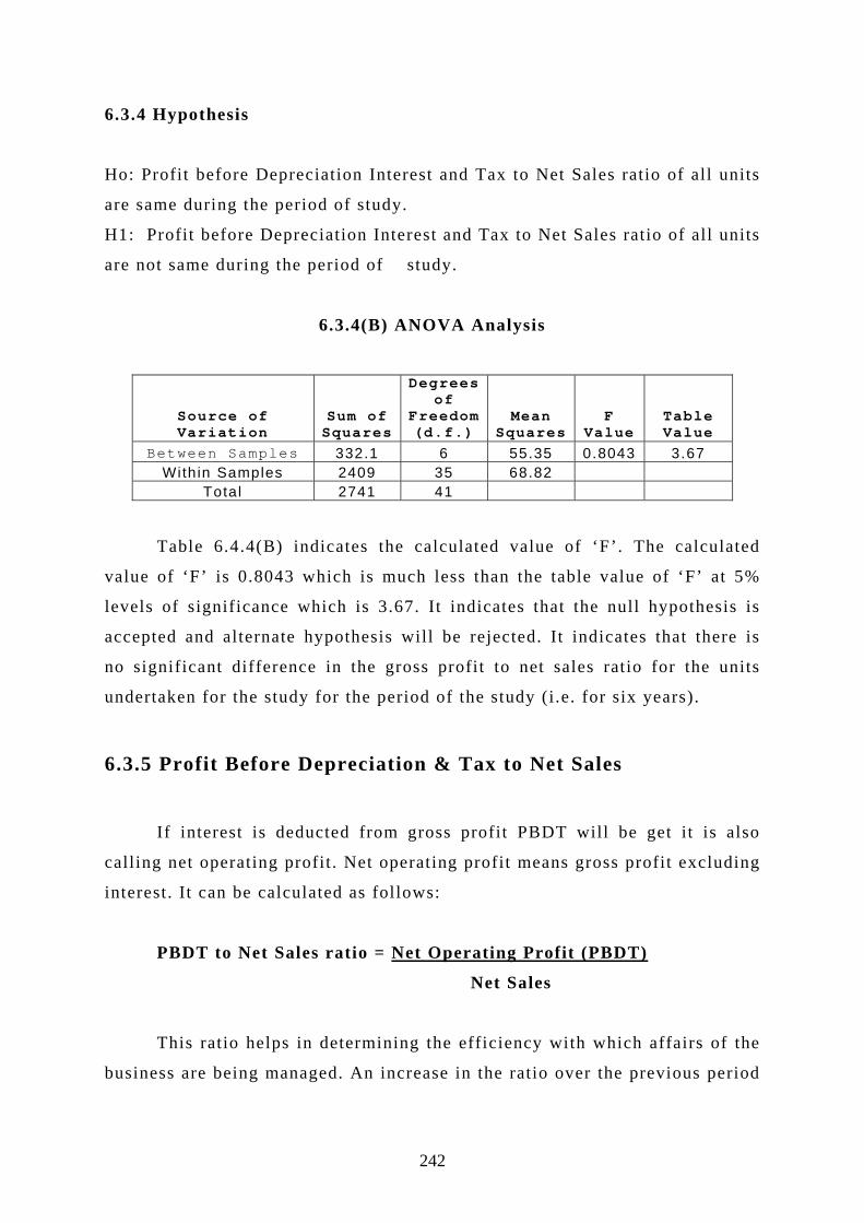
6.3.4 Hypothesis
Ho: Profit before Depreciation Interest and Tax to Net Sales ratio of all units
are same during the period of study.
H1: Profit before Depreciation Interest and Tax to Net Sales ratio of all units
are not same during the period of study.
6.3.4(B) ANOVA Analysis
Source of Variation
Sum of Squares
Degrees of
Freedom (d.f.)
Mean Squares
F Value
Table Value
Between Samples 332.1 6 55.35 0.8043 3.67 With in Samples 2409 35 68.82
Total 2741 41
Table 6.4.4(B) indicates the calculated value of ‘F’. The calculated
value of ‘F’ is 0.8043 which is much less than the table value of ‘F’ at 5%
levels of significance which is 3.67. It indicates that the null hypothesis is
accepted and alternate hypothesis will be rejected. It indicates that there is
no significant difference in the gross profit to net sales ratio for the units
undertaken for the study for the period of the study (i.e. for six years).
6.3.5 Profit Before Depreciation & Tax to Net Sales
If interest is deducted from gross profit PBDT will be get it is also
calling net operating profit . Net operating profit means gross profit excluding
interest. It can be calculated as follows:
PBDT to Net Sales ratio = Net Operating Profit (PBDT)
Net Sales
This ratio helps in determining the efficiency with which affairs of the
business are being managed. An increase in the ratio over the previous period
242

indicates improvement in the operational efficiency of the business, provided
the gross profit ratio is constant. The ratio is thus an effective measure to
check the profitability of business.
An investor has to judge the adequacy or otherwise of this ratio by
taking into account the cost of capital, the return in the industry as a whole
and market conditions such as boom or depression period. No norms can be
laid down. However, constant increase in the above ratio year after year is a
definite indication of improving conditions of the business( 1 0 ).
Table 6.3.5(A)
PBDT to Net Sales Ratio Table
REFINERIES YEAR BPCL HPCL IOC MRP BRP KRL CPCL Overall Trend
Mar-98 11.2 6.61 5.01 11.12 12.21 7.86 7.606 8.81 Mar-99 5.89 6.78 6.86 5.01 7.11 12.63 9. 4 7.62 Mar-00 5.34 5.23 5.94 -5.72 4.79 5.61 4.71 3.7 Mar-01 4.15 3.75 3.53 -3.46 -3.09 2.59 3.03 1.5 Mar-02 5.3 4.34 6.06 -8.36 -21.6 3.77 2.53 -1.14 Mar-03 5.65 6.02 8.81 -3.62 16.73 8.41 7 7 Average 6.26 5.46 6.04 -0.84 2.69 6.81 5.66 (Source: Annual reports of the companies 1998-2003)
Table 6.3.5(A) indicates the Profit before Depreciation and Taxes to
Net Sales ratio of sampled refineries which indicates the relationship between
Net Operating Profit to Net Sales. The data was for six years. For BPCL this
ratio shows decreasing trends it was 11.20, 5.89, 5.34, 4.15, 5.30 and 5.65 for
the respective year of 1998, 1999, 2000, 2001, 2002 and 2003. For HPCL it
was 6.61, 6.78, 5.23, 3.75, 4.34 and 6.02 for the respective years of 1998,
1999, 2000, 2001, 2002 and 2003. This ratio of HPCL shows mixed trends.
For IOC the ratio of sampled units’ shows mixed trends. The ratio ware 5.01,
6.86, 5.94, 3.53, 6.06 and 8.81 for the respective years from 1998, 1999,
2000, 2001, 2002 and 2003. For MRP the ratio were 11.12, 5.01, -5.72, -3.46,
-8.36 and -3.62 for the respective years of 1998, 1999, 2000, 2001, 2002 and
2003. It shows decreasing trends. For BRP ratio was 12.21, 7.11, 4.79, -3.09,
-21.60 and 16.73 for the year 1998, 1999, 2000, 2001, 2002 and 2003. It
243

shows mixed trends. For KRL it was 7.86, 12.63, 5.61, 2.59, 3.77, and 8.41
respective years of 1998, 1999, 2000, 2001, 2002 and 2003. It shows mixed
trends. For CPCL it was 7.66, 9.04, 4.71, 3.03, 2.53, and 7.00 respective
years of 1998, 1999, 2000, 2001, 2002 and 2003. It shows mixed trends. The
average of PBDT to Net sales ratio of BPCL units is 6.26, HPCL is 5.46,
IOC is 6.04, MRP is -0.84, BRP is 2.69, KRL is 6.81 and CPCL is 5.86.
Further over all trend of the same ratio of all the units undertaken for the
study is for the year ending 1998 is 8.81, for the year ending 1999 is 7.62,
for the year ending 2000 is 3.70, for the year ending 2001 is 1.50, for the
year ending 2002 is -1.14 and for the year ending 2003 is 7.00.
Figure 6.3.5
PBDT / NET SALES
-25-20-15-10-505
101520
1998 1999 2000 2001 2002 2003
YEARS
RATI
O (T
IMES
)
BPCLHPCLIOCMRPBRPKRLCPCL
The figure 6.3.5 shows the trend of net operating profit margin ratio.
The trend of net operating profit margin ratio is having almost same trend
as the gross profit margin ratio. HPCL, BPCL, CPCL has decreased their net
operating profit with less fluctuations. MRP and BRP has very low margin
ratio of gross profit also but after deducting interest i t became very law. It
means they have burden of interest charges. But BRP has improved its
efficiency of profit earning in the year 2003. Performance of MRP is very
poor. It has heavy interest burden. Overall trend of the same ratio of the
244

industry undertaken for the study has also high fluctuation because of MRP
and BRP unit. IOC and KRL have improved their profitability during the
period of study. IOC is the best in the net operating profit among all other
units.
6.3.5 Hypothesis
Ho: Profit before Depreciation and Tax to Net Sales ratio of all units are
same during the period of study.
H1: Profit before Depreciation Tax to Net Sales ratio of all units are not same
during the period of study.
6.3.5(B) ANOVA Analysis
Source of Variation
Sum of Squares
Degrees of
Freedom (d.f.)
Mean Squares
F Value
Table Value
Between Samples 268.6 6 44.76 1.15 3.67 With in Samples 1363 35 38.93
Total 1631 41
Table 6.3.5(B) indicates the calculated value of ‘F’. The calculated
value of ‘F’ is 1.150 which is much less than the table value of ‘F’ at 5%
level of significance which is 3.67. It indicates that the null hypothesis is
accepted and alternate hypothesis will be rejected. It indicates that there is
no significant difference in net operating profit to net sales in the units
undertaken for the study for the research period of the study (i.e. for six
years). It can be concluded that there is no difference in the net profit margin
ratio regarding to sales.
245

6.3.6 Profit after Tax to Net Sales Ratio
This is the ratio of net profit to net sales. Here profit is calculated by
deducting taxes, interest and depreciation from gross profit . It is computed as
follows:
Net Profit Ratio = Net Profit (Profit After Tax) * 100
Net Sales
The concept of net profit is different from net operating profit . In
calculating the net profit all non – operating expenses and losses are
deducted and all non – operating incomes are added. Taxes are also deducted
for calculating the net profit . The net profit ratio is the overall measure of a
firm’s ability to turn each rupee of sales into profit . It indicates the
efficiency with which a business is managed. A firm with a high net profit
ratio is in an advantageous position to survive in the face of rising cost of
production and falling selling prices( 1 1 ). Where the net profit ratio is low the
firm will find it difficult to with stead these types of adverse conditions.
Comparison of net profit ratio with other firms in the same industry or with
the previous years will indicate the scope for improvement. This will enable
the firm to maximize its efficiency.
Table 6.3.6(A)
PAT to Net Sales Ratio Table
REFINERIES YEAR BPCL HPCL IOC MRP BRP KRL CPCL Overall Trend
Mar-98 5.45 3.3 2.53 1.93 8.87 5.13 4.16 4.48 Mar-99 2.95 3.49 4.33 -0.4 3.98 7.8 5.16 3.9 Mar-00 2.44 3.51 2.93 -10.26 2.61 3.78 2.45 1.07 Mar-01 1.87 2.28 2.22 -9.39 -5.47 1.14 1.2 -0.88 Mar-02 2.56 1.98 3.04 -15.21 -24.19 1.14 0.9 -4.25 Mar-03 2.87 3.1 5.24 -8.07 8.83 4.73 3.63 2.9 Average 3.02 2.94 3.38 -6.9 -0.9 3.95 2.92 (Source: Annual reports of the companies 1998-2003)
246

Table 6.3.6(A) indicates the Profit after Tax to Net Sales ratio of
sampled refineries indicates the relationship between Profit After Tax to Net
Sales. The data was for six years. For BPCL this ratio shows mixed trends it
was 5.45, 2.95, 2.44, 1.87, 2.56 and 2.87 for the respective year of 1998,
1999, 2000, 2001, 2002 and 2003. For HPCL it was 3.30, 3.49, 3.51, 2.28,
1.98 and 3.10 for the respective years of 1998, 1999, 2000, 2001, 2002 and
2003. This ratio of HPCL shows steady trends. For IOC the ratio of sampled
units’ shows increasing trends. The ratio ware 2.53, 4.33, 2.93, 2.22, 3.04
and 5.24 for the respective years from 1998, 1999, 2000, 2001, 2002 and
2003. For MRP the ratio were 1.93, -0.4, -10.26, -9.39, -15.21 and -8.07or
the respective years of 1998, 1999, 2000, 2001, 2002 and 2003. It shows
decreasing trends. For BRP ratio was 8.87, 3.98, 2.61, -5.47, -24.19 and 8.83
for the year 1998, 1999, 2000, 2001, 2002 and 2003. It shows mixed trends.
For KRL it was 5.13, 7.80, 3.78, 1.14, 1.14, and 4.73 respective years of
1998, 1999, 2000, 2001, 2002 and 2003. It shows mixed trends. For CPCL it
was 4.16, 5.16, 2.45, 1.20, 0.90, and 3.63 respective years of 1998, 1999,
2000, 2001, 2002 and 2003. It shows mixed trends. The average of profit
after tax to net sales ratio is 3.02, HPCL is 2.94, I OC i s 3 . 38 , MRP i s -
6 .90 , BRP i s -0.90, KRL is 3.95 and CPCL is 2.92. Further over all trend of
the same ratio of all the units undertaken for the study is for the year ending
1998 is 4.48, for the year ending 1999 is 3.90, for the year ending 2000 is
1.07, for the year ending 2001 is -0.88, for the year ending 2002 is -4.25 and
for the year ending 2003 is 2.90.
247

Figure 6.3.6
PAT (NNRT) / NET SALES
-30-25-20-15-10-505
1015
1998 1999 2000 2001 2002 2003
YEAR
RATI
O (T
IMES
)
BPCLHPCLIOCMRPBRPKRLCPCL
The figure 6.3.6 shows the trend of net profitability margin ratio. The
trend of net profit margin ratio is having almost same trend as the gross
profit margin ratio and operating profit margin ratio. HPCL, BPCL, CPCL
has decreased their net profit with less fluctuations. KRL has increasing
trend for gross profit margin ratio and operating profit margin ratio but here
it decreases so it can be said that i t has more tax burden. MRP and BRP has
very low margin ratio of net profit . But Both have improved its efficiency of
profit earning in the year 2003. Overall trend for the same of the industry
undertaken for the study has also high fluctuation because of fluctuation in
MRP and BRP unit. IOC has improved their profitability during the period of
study. IOC is the best in the net profit among all other units.
6.3.6 Hypothesis
Ho: Ratio of Profit after Tax to Net Sales ratio of all units is same during the
period of study.
H1: Ratio of Profit after Tax to Net Sales ratio of all units is not same during
the period of study.
248

6.3.6(B) ANOVA Analysis
Source of Variation
Sum of Squares
Degrees of
Freedom (d.f.)
Mean Squares
F Value Table Value
Between Samples 549.9 6 91.65 3.022 3.67 With in Samples 1061 35 30.32
Total 1611 41
Table 6.3.6(B) indicates the calculated value of ‘F’. The calculated
value of ‘F’ is 3.022 which is less than the table value of ‘F’ at 5% levels of
significance which is 3.67. It indicates that the null hypothesis is accepted
and alternate hypothesis will rejected. It indicates that there is no
significance difference in the net profit to sales ratio in the units undertaken
for the study for the research period of the study (i .e. for six years). Each
unit is following same pattern of cost of goods and selling price so their
profitability analysis also shows that there is no difference in the same ratio.
.
B. Return Ratios
The strategic aim of a business enterprise is to earn a return on capital.
If, in any particular case, the return in the long term is not satisfactory than
the deficiency should be corrected of\r the activity be abandoned for a more
favorable one. The return ratios should be calculated for measuring the
historical performance of an investment center calls for a comparison of the
profit that has been earned with capital employed.
6.3.7 Profit after Tax to Net Worth Ratio
This is known as Return on Shareholders’ Funds. Return on
shareholders’ funds is a very effective measure of the profitability of an
enterprise. These ratios measure the return on the total equity of the
shareholders. It should be compared with the ratios of other similar
249

companies to determine whether the rate of return is attractive. In fact, this
ratio is one of the most important relationships in financial statement
analysis. It shows the ratio of net profit to owners’ equity.
Return on Proprietor’s Equity = Net Profit after Taxes and Interest *100
Shareholders’ Funds
Net profit is calculated after charging interest on long term liabilities
and payment of taxes. Shareholders’ funds include equity capital, preference
capital, capital reserve, general reserve and other undistributed profits. For
the purpose of this ratio, average of the figure relating to shareholders’ funds
in the beginning and at the end of the period is taken.
Common or ordinary shareholders are entitled to the residual profits.
The rate of dividend is not fixed; the earnings may be distributed to
shareholders or retained in the business. Nevertheless, the net profits after
taxes represent their return. A return on shareholders’ equity is calculated to
see the profitability of owners’ investment. The shareholders’ equity or net
worth will include paid – up share capital, share premium and reserves and
surplus less accumulated losses. Net worth can also be found by subtracting
total liabilities from total assets( 1 2 ) .
ROE (Return on Equity) indicates how well the firm has used the
resources of owners. In fact, this ratio is one of the most important
relationships in financial analysis. The earning of a satisfactory return is the
most desirable objective of a business. The ratio of net profit to owners’
equity reflects the extent to which this objective has been accomplished. This
ratio is, thus, of great interest to the present as well as the prospective
shareholders and also of great concern to management, which has the
responsibility of maximizing the owners’ welfare.
This ratio expresses the net profit in terms of the equity shareholders
funds. This ratio is an important yardstick of performance for equity
shareholder, since it indicate the return on the funds employed by them.
250

However, this measure is based on the historical net worth and will be high
for old plants and low for new plants.
The factor which motivates shareholder to invest in a company is the
expectation of an adequate rate of return on their funds. This ratio is useful
in measuring the rate of return as a percentage of the book value of
shareholders equity( 1 3 ).
This ratio indicates how well the firm has used the resources of
owners. In fact this ratio is one of the most important relationships in
financial analysis. The earnings of satisfactory return are the most desirable
objective of a business. This ratio is thus, of great interest to the present as
well as the prospective shareholder and also of great concern to management
which has the responsibility of maximizing the owners’ welfare.
Table 6.3.7(A)
Profit after Tax to Net Worth Ratio
REFINERIES YEAR BPCL HPCL IOC MRP BRP KRL CPCL Overall Trend
Mar-98 23.44 16.21 13.41 5.52 12.67 29.81 13.36 16.35 Mar-99 24.62 17.84 23.58 -1.12 5.47 33.28 20.18 17.69 Mar-00 22 19.57 18.66 -29 5.14 18.74 12.66 9.68 Mar-01 20.67 16.89 16.67 -34.14 -11.25 6.48 7.43 3.25 Mar-02 22.55 12.92 20.12 -164.03 -72.42 5.55 5.1 -24.32 Mar-03 28.59 24.44 34.08 -106.62 49.66 35.42 26.71 13.18 Average 23.65 17.98 21.09 -54.9 -1.79 21.55 14.24 (Source: Annual reports of the companies 1998-2003)
Table 6.3.7(A) indicates the Profit after Tax to Net Worth ratio of
sampled refineries which indicates the relationship between Net Profit to Net
Worth. The data was for six years. For BPCL this ratio shows mixed trends it
was 5.45, 2.95, 2.44, 1.87, 2.56 and 2.87 for the respective year of 1998,
1999, 2000, 2001, 2002 and 2003. For HPCL it was 3.30, 3.49, 3.51, 2.28,
1.98 and 3.10 for the respective years of 1998, 1999, 2000, 2001, 2002 and
2003. This ratio of HPCL shows mixed trends. For IOC the ratio of sampled
units’ shows mixed trends. The ratio ware 2.53, 4.33, 2.93, 2.22, 3.04 and
251

5.24 for the respective years from 1998, 1999, 2000, 2001, 2002 and 2003.
For MRP the ratio were 1.93, -0.4, -10.26, -9.39, -15.21 and -8.07or the
respective years of 1998, 1999, 2000, 2001, 2002 and 2003. It shows much
decreasing trends. For BRP ratio was 8.87, 3.98, 2.61, -5.47, -24.19 and 8.83
for the year 1998, 1999, 2000, 2001, 2002 and 2003. It shows significantly
mixed trends. For KRL it was 5.13, 7.80, 3.78, 1.14, 1.14, and 4.73
respective years of 1998, 1999, 2000, 2001, 2002 and 2003. It shows mixed
trends. For CPCL it was 4.16, 5.16, 2.45, 1.20, 0.90, and 3.63 respective
years of 1998, 1999, 2000, 2001, 2002 and 2003. It shows mixed trends. The
average of profit after tax to net worth ratio of BPCL units is 23.65, HPCL is
17.98, IOC is 21.09, MRP is -54.90, BRP is -1.79, KRL is 21.55 and CPCL is
14.24. Further over all trend of the same ratio of all the units undertaken for
the study is for the year ending 1998 is 16.35, for the year ending 1999 is
17.69, for the year ending 2000 is 9.68, for the year ending 2001 is 3.25, for
the year ending 2002 is -24.32 and for the year ending 2003 is 13.18.
Figure 6.3.7
Profit After Tax to Net Worth Ratio
-200
-150
-100
-50
0
50
100
1998 1999 2000 2001 2002 2003
YEARS
RATI
O
BPCLHPCLIOCMRPBRPKRLCPCL
Figure 6.3.7 shows that it can be seen that BPCL, HPCL, IOC, KRL
and CPCL have improved their profitability performance. Their return on
equity increases in 2003 compared to 1998, though they have very much
fluctuations in the trend. They have fluctuating trend but however they have
252

improvement in their net profit earning performance in 2003 compared to
1998. MRP and BRP have high fluctuation with steep fall in their
profitability ratio. Both have very poor performance which is very risky for
their investors. But however in 2003 they have better performance and their
ratio turns high in 2003 compared to their previous years. IOC is the best to
earn the return on its equity with steady performance. Overall trend of the
industry is poor in 2002 is also because of these two units. KRL has the
highest average of the ratio than other units.
6.3.7 Hypothesis
Ho: Ratio of Profit after Tax to net Worth ratio of all units are same during
the period of study.
H1: Ratio of Profit after Tax to Net Worth ratio of all units are not same
during the period of study.
6.3.7(B) ANOVA Analysis
Source of Variation
Sum of Squares
Degrees of Freedom (d.f.)
Mean Squares
F Value
Table Value
Between Samples 33500 6 5590 4.873 3.67
With in Samples 40200 35 1147 Total 7.3688E+04 41
Table 6.3.7(B) indicates the calculated value of ‘F’. The calculated
value of ‘F’ is 4.873 which is much higher than the table value of ‘F’ at 5%
levels of significance which is 3.67. It indicates that the null hypothesis is
rejected and alternate hypothesis will remain. It indicates that there is
significant difference in the profit after sales to net sales ratio in the units
undertaken for the study for the period of the study (i.e. for six years). There
is difference on return on equity of shareholders’ funds.
253

6.3.8 Profit after Tax to Total Assets
This ratio is computed to know the productivity of the total assets. This
ratio is calculated as follows:
PAT to Total Assets = Profit after Tax * 100
Total Assets
The profitability of the firm is measured by establishing relation of net
profit which is also called profit after tax with the total assets of the
organization. This ratio is indicates the efficiency of utilization of assets in
generating revenue.
Table 6.3.8(A)
Profit After Tax to Total Assets Ratio Table
REFINERIES YEAR BPCL HPCL IOC MRP BRP KRL CPCL Overal l Trend
Mar-98 9.28 8.22 4.1 0.45 9.31 8.19 2.47 6 Mar-99 9.88 9.76 8.33 -0.15 4.11 8.87 3.59 6.34 Mar-00 7.96 9.43 6.2 -4.91 3.85 4.78 3.04 4.34 Mar-01 6.36 7.36 4.98 -3.92 -7.84 1.66 3.02 1.66 Mar-02 6.56 5.34 5.85 -10.59 -33.58 1.72 1.84 -3.27 Mar-03 8.21 9.48 10.55 -8.23 15.5 13.29 7.75 8.08 Average 8.04 8.27 6.67 -4.56 -1.44 6.42 3.62 (Source: Annual reports of the companies 1998-2003)
Table 6.3.8(A) indicates the Profit after tax to Total Assets ratio of
sampled refineries which indicates the relationship between Net Profit to
Total Assets. The data was for six years. For BPCL this ratio shows mixed
trends it was 5.45, 2.95, 2.44, 1.87, 2.56 and 2.87 for the respective year of
1998, 1999, 2000, 2001, 2002 and 2003. For HPCL it was 3.30, 3.49, 3.51,
2.28, 1.98 and 3.10 for the respective years of 1998, 1999, 2000, 2001, 2002
and 2003. This ratio of HPCL shows mixed trends. For IOC the ratio of
sampled units’ shows increasing trends. The ratio ware 2.53, 4.33, 2.93, 2.22,
3.04 and 5.24 for the respective years from 1998, 1999, 2000, 2001, 2002 and
2003. For MRP the ratio were 1.93, -0.4, -10.26, -9.39, -15.21 and -8.07or
254

the respective years of 1998, 1999, 2000, 2001, 2002 and 2003. It shows
decreasing trends. For BRP ratio was 8.87, 3.98, 2.61, -5.47, -24.19 and 8.83
for the year 1998, 1999, 2000, 2001, 2002 and 2003. It shows significant
mixed trends. For KRL it was 5.13, 7.80, 3.78, 1.14, 1.14, and 4.73
respective years of 1998, 1999, 2000, 2001, 2002 and 2003. It shows mixed
trends. For CPCL it was 4.16, 5.16, 2.45, 1.20, 0.90, and 3.63 respective
years of 1998, 1999, 2000, 2001, 2002 and 2003. It shows mixed trends. The
average of profit after tax to total assets ratio of BPCL units is 8.04, HPC L
i s 8 . 27 , IOC i s 6 . 67 , MRP i s - 4 . 56 , BRP is -1.44, KRL is 6.42 and CPCL
is 3.62. Further over all trend of the same ratio of all the units undertaken for
the study is for the year ending 1998 is 6.00, for the year ending 1999 is
6.34, for the year ending 2000 is 4.34, for the year ending 2001 is 1.66, for
the year ending 2002 is -3.27 and for the year ending 2003 is 8.08.
Figure 6.3.8
Profit After Tax / Total Assets
-40
-30
-20
-10
0
10
20
1998 1999 2000 2001 2002 2003
YEARS
RATI
O
BPCLHPCLIOCMRPBRPKRLCPCL
Figure 6.3.8 shows that like all other previous ratio for thus ratio also
MRP and BRP have very high fluctuation during the period of the study.
They have not utilized their assets properly to generate profit . The ratio by
calculating net profit with total assets is going very low (in minus). It can be
concluded that assets may be unutilized or for any other reason, earning of
profit is very law. Because of these units the industry is also having mixed
255

trend. HPCL,IOC, KRL and CPCL are having improvement in the ratio. Their
assets have been util ized properly so that their ratios also increase. BPCL has
a very little fall in the ratio.
6.3.8 Hypothesis
Ho: Profit after Tax to Total Assets ratio of all units are same during the
period of study.
H1: Profit after Tax to Total Assets ratio of all units is not same during the
period of study.
6.3.8(B) ANOVA Analysis
Source of Variat ion
Sum of Squares
Degrees of Freedom
(d.f . ) Mean
Squares F
Value Table Value
Between Samples 168000 6 2.79E+04 1.004 3.67
Within Samples 974000 35 2.78E+04 Total 1 .1415E+06 41
Table 6.3.8(B) indicates the calculated value of ‘F’. The calculated
value of ‘F’ is 1.004 which is less than the table value of ‘F’ at 5% levels of
significance which is 3.67. It indicates that the null hypothesis is accepted
and alternate hypothesis will rejected. It indicates that there is no significant
difference in the profitability in relation to sale in the sampled units for the
research period. They have utilized their assets similarly to earn the net
profit .
6.3.9 Profit Before Interest and Tax to Capital Employed
This is the most important test of profitability of a business. It
measures the overall profitability. It is ascertained by comparing profit
earned and capital (or funds) employed to earn it . It is also called as ‘Return
on Investment’ on capital employed. It indicates percentage of return on the
256

total capital employed in the business. It is calculated on the basis of the
following formula:
PBIT to Capital Employed = Operating Profit (PBIT) * 100
Capital Employed
The term capital employed has been given different meaning by
different accountants. Some of the popular meanings are as follows:
o Sum – Total of all assets whether fixed or current.
o Sum – Total of fixed assets.
o Sum – Total of long term funds employed in the business i .e. share
capital + long term loan – (Non business assets + Fictitious assets)
The term capital employed can also be computed as follows:
Equity Share Capital + Preference Share Capital + Reserves and other
Undistributed Profits + Long term loans and Debentures - Fictitious Assets
(e.g. Preliminary Expenses) - Non–operating Assets (e.g. Investments).
Or the term capital Employed may also be computed in the following way;
Fixed Assets Cost – Depreciation + Net Working Capital (i .e. current
assets minus current liabilities and provisions)
The term ‘Operating Profit’ means Profit before Interest and Tax. The
term interest means ‘Interest on Long – Term Borrowing’. Interest on short –
term borrowing will be deducted for computing operating profit . Non trading
losses or expenses such as loss on account of fire etc. will also be
excluded( 1 4 ).
Thus, the return on capital employed is dependent upon two factors,
viz. (1) net profit ratio, and (2) capital turnover ratio.
257

ROI is the only ratio which measures satisfactorily the overall
performance of a business from the point of view of profitability. This ratio
indicates how well the management has utilized the fund supplied by the
owners and creditors. In other words this ratio is intended to measure the
earning power of the net assets of the business. The higher the ROI, the more
efficient the management is considered to be in using the funds available. In
fact, this ratio can also be advantageously used in judging the performance
efficiency of different firms in different industries. Management also uses
this ratio for decision making purposes( 1 4 ).
Table 6.3.9(A)
Profit Before Interest and Tax to Capital Employed Ratio Table
COMPANIES YEAR BPCL HPCL IOC MRP BRP KRL CPCL Overall Trend
Mar-98 23.71 18.33 17.93 12.62 14.1 30.07 15.22 18.85 Mar-99 28.38 23.04 28.71 7.18 6.38 34.04 19.58 21.04 Mar-00 24.69 21.05 19.9 -0.02 6.68 15.66 12.76 14.39 Mar-01 22.39 19.02 14.26 -0.68 -9.65 9.3 10.63 9.32 Mar-02 30.43 20.83 32.05 -2.53 -90.25 12.55 9.55 1.8 Mar-03 35.4 32.66 39.57 -0.22 79.98 38.73 21.15 35.32 Average 27.5 22.49 25.4 2.73 1.21 23.39 14.82 (Source: Annual reports of the companies 1998-2003)
Table 6.3.9(A) indicates the Profit before interest and tax to Capital
Employed ratio of sampled refineries which indicates the relationship
between Net Operating Profit with Capital Employed in the firm. The data
was for six years. For BPCL this ratio shows increasing trends it was 5.45,
2.95, 2.44, 1.87, 2.56 and 2.87 for the respective year of 1998, 1999, 2000,
2001, 2002 and 2003. For HPCL it was 3.30, 3.49, 3.51, 2.28, 1.98 and 3.10
for the respective years of 1998, 1999, 2000, 2001, 2002 and 2003. This ratio
of HPCL shows increasing trends. For IOC the ratio of sampled units’ shows
mixed trends. The ratio ware 2.53, 4.33, 2.93, 2.22, 3.04 and 5.24 for the
respective years from 1998, 1999, 2000, 2001, 2002 and 2003. For MRP the
ratio were 1.93, -0.4, -10.26, -9.39, -15.21 and -8.07or the respective years of
1998, 1999, 2000, 2001, 2002 and 2003. It shows decreasing trends. For BRP
ratio was 8.87, 3.98, 2.61, -5.47, -24.19 and 8.83 for the year 1998, 1999,
258

2000, 2001, 2002 and 2003. It shows significant changes. For KRL it was
5.13, 7.80, 3.78, 1.14, 1.14, and 4.73 respective years of 1998, 1999, 2000,
2001, 2002 and 2003. It shows mixed trends. For CPCL it was 4.16, 5.16,
2.45, 1.20, 0.90, and 3.63 respective years of 1998, 1999, 2000, 2001, 2002
and 2003. It shows mixed trends. The average ratio of incremental growth of
value of production to total assets of BPCL units is 27.50, HPCL is 22.49,
IOC is 25.40, MRP is 2.73, BRP is 1.21, KRL is 23.39 and CPCL is 14.82.
Further over all trend of the same ratio of all the units undertaken for the
study is for the year ending 1998 is 18.85, for the year ending 1999 is 21.04,
for the year ending 2000 is 14.39, for the year ending 2001 is 9.32, for the
year ending 2002 is 1.80 and for the year ending 2003 is 35.32.
Figure 6.3.9
PBIT / Capital Employed
-100
-50
0
50
100
1998 1999 2000 2001 2002 2003
YEARS
RATI
O
BPCLHPCLIOCMRPBRPKRLCPCL
Figure 6.3.9 shows that all the units except BRP and MRP have
increased their return on investment. Though the ratios of all the units are
fluctuating during the research period but they have improved in the year
2003 compared to the year 1998. Among them IOC has performed best to earn
the return on capital employed. It proves its overall efficiency of the firm.
BRP has good ratio in the year 2003 but it was very fluctuating during the
period of study. BRP has improved a lot and has got a powerful return. Its
259

return to the total capital is highest than all other units. Because of that only
the ratio of overall industry went high in the year 2003. But investors should
analyses the causes of very high fluctuations. MRP has very poor
performance among all other units.
6.3.9 Hypothesis
Ho: Profit before Interest and Tax to Capital Employed ratio of all units are
same during the period of study.
H1: Profit before Interest and Tax to Capital Employed ratio of all units are
not same during the period of study.
6.3.9(B) ANOVA Analysis
Source of Variation
Sum of Squares
Degrees of Freedom (d.f .)
Mean Squares
F Value
Table Value
Between Samples 4257 6 709.5 1.488 3.67
With in Samples 16700 35 476.8 total 2 .0946E+04 41
Table 6.3.9(B) indicates the calculated value of ‘F’. The calculated
value of ‘F’ is 1.488 which is less than the table value of ‘F’ at 5% levels of
significance which is 3.67. It indicates that the null hypothesis is accepted
and alternate hypothesis will rejected. It indicates that there is no significant
difference for the return on investment to capital employed in the units
undertaken for the study for the period of the study (i.e. for six years). It can
be concluded that there is not any differences in the earning efficiency of the
sampled units. All have same trend of profitability performance.
6.3.10 Profit After Tax to Capital Employed
The fund employed in net assets is known as capital employed. Net
assets plus current assets minus current liability excluded bank loans. PAT
represents residue income of shareholder. It can compute as follow:
260

PAT to Capital Employed = Profit After Tax * 100
Capital Employed
Return on capital employed provides a strong incentive for optimal
utilization. This encourages managers to obtain assets that will provide a
satisfactory return on investment and to dispose of assets that are not
providing an acceptable return.
Table 6.3.10(A)
Profit After Tax to Capital Employed Ratio Table
COMPANIES YEAR BPCL HPCL IOC MRP BRP KRL CPCL Overal l Trend
Mar-98 15.23 12.14 8.7 0.69 11.01 20.07 6.4 10.61 Mar-99 17.06 14.39 17.45 -0.17 4.87 21.08 10.21 12.13 Mar-00 15.56 15.63 12.18 -5.55 5.06 11.35 6.51 8.68 Mar-01 13.15 11.9 8.01 -5.14 -11.87 3.9 3.73 3.38 Mar-02 16.22 10.9 15.6 -15.12 -102.96 3.72 2.61 -9.86 Mar-03 19.89 19.57 25.8 -12.51 42.7 22.32 10.85 18.37 Average 16.19 14.09 14.62 -6.3 -8.53 13.74 6.72 (Source: Annual reports of the companies 1998-2003)
Table 6.3.10(A) indicates the Profit after Tax to Capital Employed
ratio of sampled refineries which indicates the relationship between Net
Profit with Capital Employed of the firm. The data was for six years. For
BPCL this ratio shows increasing trends it was 5.45, 2.95, 2.44, 1.87, 2.56
and 2.87 for the respective year of 1998, 1999, 2000, 2001, 2002 and 2003.
For HPCL it was 3.30, 3.49, 3.51, 2.28, 1.98 and 3.10 for the respective years
of 1998, 1999, 2000, 2001, 2002 and 2003. This ratio of HPCL shows mixed
trends. For IOC the ratio of sampled units’ shows increasing trends. The ratio
ware 2.53, 4.33, 2.93, 2.22, 3.04 and 5.24 for the respective years from 1998,
1999, 2000, 2001, 2002 and 2003. For MRP the ratio were 1.93, -0.4, -10.26,
-9.39, -15.21 and -8.07or the respective years of 1998, 1999, 2000, 2001,
2002 and 2003. It shows decreasing trends. For BRP ratio was 8.87, 3.98,
2.61, -5.47, -24.19 and 8.83 for the year 1998, 1999, 2000, 2001, 2002 and
2003. It shows significantly mixed trends. For KRL it was 5.13, 7.80, 3.78,
1.14, 1.14, and 4.73 respective years of 1998, 1999, 2000, 2001, 2002 and
261

2003. It shows mixed trends. For CPCL it was 4.16, 5.16, 2.45, 1.20, 0.90,
and 3.63 respective years of 1998, 1999, 2000, 2001, 2002 and 2003. It shows
mixed trends. The average of profit after tax to capital employed ratio of
BPCL units is 16.19, HPCL is 14.09, IOC is 14.62, MRP is -6.30, BRP is -
8.53, KRL is 13.74 and CPCL is 6.72. Further over all trend of the same ratio
of all the units undertaken for the study is for the year ending 1998 is 10.61,
for the year ending 1999 is 12.13, for the year ending 2000 is 8.68, for the
year ending 2001 is 3.38, for the year ending 2002 is -9.86 and for the year
ending 2003 is 18.37.
Figure 6.3.10
PAT / Capital Employed
-120-100-80-60-40-20
0204060
1998 1999 2000 2001 2002 2003
YEARS
RATI
O
BPCLHPCLIOCMRPBRPKRLCPCL
Figure 6.3.10 shows that all the units except BRP and MRP have
increased their return on capital employed which provides strong incentives
for optimal utilization. Though the ratios are fluctuating during the research
period but it has improved in the year 2003 compared to the year 1998 in all
those units. Among them IOC has performed best to earn the return on capital
employed and used their assets’ optimal utilization. Further it has more
residue income for shareholders. It proves its overall efficiency of the firm.
BRP has good ratio in the year 2003 but it was very fluctuating during the
period of study. BRP has improved a lot and has got a powerful return. Its
262

263
return to the total capital is highest than all other units in the year 2003.
Because of that only the ratio of overall industry went high in the year 2003.
But investors should analyses the causes of very high fluctuations of BRP.
MRP has very poor performance among all other units.
6.3.10 Hypothesis
Ho: Profit after Tax to Capital Employed ratio of all units are same
during the period of study.
H1: Profit after Tax to Capital Employed ratio of all units are not same
during the period of study.
6.3.10(B) ANOVA Analysis
Source of Variat ion
Sum of Squares
Degrees of Freedom
(d.f . ) Mean
Squares F
Value Table Value
Between Samples 3937 6 656.2 1.737 3.67
Within Samples 13200 35 377.8 to tal 1 .7160E+04 41
Table 6.3.10(B) indicates the calculated value of ‘F’. The calculated
value of ‘F’ is 1.737 which is less than the table value of ‘F’ at 5% levels of
significance which is 3.67. It indicates that the null hypothesis is accepted
and alternate hypothesis will be rejected. It indicates that there is no
significance difference in the return on investment to capital employed in the
units undertaken for the study for the period of the study (i.e. for six years).
All the units have same trend of earning return on net assets and having same
kind of profitability performance.

References:-
1. Icfaian journal of Management Research – October (2006) Pg. 74
2. Pandey I M – Financial Management – Vikas Publishing House Pvt. Ltd
– 8t h Edition (1999) Pg. 133
3. M.N.Arora – Cost and Management Accounting – Theory and Problems
- Himalaya Publishing House – 1st Edition – (2004) Pg. 14.15
4. Ravi M Kishore – Cost and Management Accounting – BPB Publication
2nd Edition (1990) Pg. 178
5. Pandey I. M – Financial Management – Vikas Publishing House Pvt Ltd
– 8t h Edition (1999) Pg. 134
6. M.N.Arora – Cost and Management Accounting – Theory and Problems –
Himalaya Publishing House – 1s t Edition (2004) Pg. 14.16
7. Prasanna Chandra – Financial Performance – Indian Institute of
Management – (June 2002) Pg.78
8. Pandey I M – Financial Management – Vikas Publishing House Pvt. Ltd
– 8t h Edition (1999) Pg. 135
9. Dr. S.N. Maheshwari – Management Accounting And Financial Control –
Sultan Chand & Sons – 9t h Edition Pg. B-39
10.Dr. S.N. Maheshwari – Management Accounting And Financial Control –
Sultan Chand & Sons – 9t h Edition Pg. B-40
11.Pandey I. M – Financial Management – Vikas Publishing House Pvt
Ltd – 8t h Edition 1999 Pg. 132
12.Pandey I. M – Financial Management – Vikas Publishing House PVT
Ltd – 8t h Edition 1999 Pg. 139
13.Khan M.Y.and Jain P. K. - Financial Management - Tata Mc.Graw Hill
Publishing Co. (1990) Pg. 167
264

14.Dr. S.N. Maheshwari – Management Accounting And Financial Control –
Sultan Chand & Sons – 9t h Edition Pg. B-32
15.M.N.Arora – Cost and Management Accounting – Theory and Problems –
Himalaya Publishing House – (First Edition-2004) Pg. 14.21
265

CHAPTER 7
COMPARISON OF PERFORMANCE AND EVALUATION OF SAMPLED
UNITS
7.1 Introduction
7.1.1 Correlation matrix of BPCL
7.1.2 Factor analysis of BPCL
7.2.1 Correlation matrix of HPCL
7.2.2 Factor analysis of HPCL
7.3.1 Correlation matrix of IOC
7.3.2 Factor analysis of IOC
7.4.1 Correlation matrix of MRP
7.4.2 Factor analysis of MRP
7.5.1 Correlation matrix of BRP
7.5.2 Factor analysis of BRP
7.6.1 Correlation matrix of KRL
7.6.2 Factor analysis of KRL
7.7.1 Correlation matrix of CPCL
7.7.2 Factor analysis of CPCL
266

CHAPTER 7
COMPARISON OF PERFORMANCE AND EVALUATION OF
SAMPLED UNITS
7.1 Introduction
All statically techniques which simultaneously analyses more than two
variables can be categories as ‘multivariate techniques’ or multivariable
analyze it is a collection of methods for analyzing data in which a number of
observation are available for each object. These techniques take account of
the various relationships among variable. This is a powerful tool to analyze
data represented in terms of many variables. These techniques are largely
empirical and deal with the reality( 1 ) . They possess the ability to analyze
complex data. Accordingly in most of the applied and behavioral researches,
researcher generally resort to multivariate analyze techniques for realistic
results( 1 ) . Besides being a tool for analyzing the data, multivariate techniques
also help in various types of decision making.
Today, there exist a great variety of multivariate techniques. Here, the
researcher has used the centroid method of factor analysis techniques. It is
developed by L.L.Thurstone. This technique allows the researcher to group
variables into factors (based on correlation between variables) and the factors
so derived may be treated as new variables (often termed as latent variables)
and their value derived by summing up the values of original variable which
have been grouped into the factor( 2 ) . Since the factors happen to be linear
combinations of data, the co-ordinates of each observation or variable is
measured to obtain what are called factor loading. Such factor loadings
represent the correlation between the particular variables and the factor and
are usually place in a matrix of correlation between the variable and the
factor. When there are two or more than two independent variables present in
the data, the analysis concerning relationship is known as multiple
correlations. And the table generates is called multiple correlation matrix.
267

268
Thus the researcher has first generates the correlation matrix and then
centroid method of factor analysis has been used to find the loading factors.
The centroid method tends to maximize the sum of loadings,
disregarding the sign. It is method which extracts the largest sum of absolute
loadings for each factor in turn. It is defined by the linear combinations in
which all weights are either +1.0 or -1.0( 3 ) .
7.1.1 Correlation matrix of BPCL
Here, Table 7.1.1 table shows the correlation matrix of the 22 ratios of
various variables of the firm BPCL. Ratios have been calculated from the
data for the period of study 1998-2003. From the table, relation between the
various ratios and the degree of relation between them can be found out here.

269
Table 7.1.1 Correlation between the ratios of BPCL
VOP To GFA
VOP To NFA
VOP To CE
VOP To CA
PBDIT To Sales
PBIT To Sales
PAT To Sales
PAT To NW
PAT To TA
PBIT To CE
PAT To CE
LTD To Equity
TD To Equity
Current Ratio
Int. Coverage
G.W.C.C
N.W.C.C
Debtor’s Ratio
Creditor’s Ratio
Raw Material Tuover
rn
Finished Goods Turnover
75 0.24 77 0.01
32 0.41
84 -0.19 43 0.66
48 0.54
43 0.50
39 0.61
32 0.23
27 0.73
23 -0.13 24 0.03
47 -0.32
20 -0.61 74 0.18 08 -0.06
78 -0.18
81 -0.05
64 0.63
22 -0.26
-0.28
28 1
Name of Ratio
VOP ToT.A.
VOP to T.A 1 VOP to GFA 0.
VOP to NFA -0
VOP to CE 0.VOP to CA 0.PBDIT to Sales -0
PBIT to Sales -0
PAT to Sales -0
PAT to N.W. 0.
PAT to T.A. -0
PBIT to CA 0.PAT to CA -0LTD to Equity -0
TD to Equity 0.Current Ratio 0.Int. Coverage -0
G.W.C.C. -0
N.W.C.C. -0
Debtors Ratio -0
Creditors Ratio -0
Raw Material turnover 0.
Finished Goods turnover
0.
0.95 -0.12 0.87 0.84 -0.46 -0.46 -0.32 0.22 -0.17 0.01 -0.01 -0.31 0.22 0.80 -0.32 -0.97 -0.69 -0.31 -0.69 0.95 1 -0.26 0.97 0.68 -0.64 -0.64 -0.49 0.17 -0.42 0.07 -0.04 -0.11 0.46 0.77 -0.32 -0.96 -0.68 -0.54 -0.66 0.
.12 -0.26 1 -0.45 -0.07 0.04 0.07 -0.02 -0.58 0.39 -0.87 -0.65 0.22 -0.33 0.18 -0.25 0.32 0.39 0.60 0.00 -0.
87 0.97 -0.45 1 0.55 -0.64 -0.63 -0.50 0.28 -0.51 0.24 0.11 -0.15 0.51 0.70 -0.17 -0.92 -0.75 -0.71 -0.51 0.84 0.68 -0.07 0.55 1 0.01 -0.03 0.14 0.40 0.22 0.13 0.16 -0.51 -0.14 0.55 -0.25 -0.82 -0.54 0.09 -0.66 0.
.46 -0.64 0.04 -0.64 0.01 1 0.99 0.98 0.53 0.87 0.39 0.59 -0.50 -0.87 -0.37 0.60 0.39 0.07 0.48 0.54 0.
.46 -0.64 0.07 -0.63 -0.03 0.99 1 0.97 0.54 0.89 0.38 0.60 -0.53 -0.91 -0.29 0.68 0.40 0.01 0.42 0.62 -0.
.32 -0.49 -0.02 -0.50 0.14 0.98 0.97 1 0.65 0.88 0.46 0.65 -0.56 -0.87 -0.22 0.64 0.23 -0.09 0.38 0.49 -0.
22 0.17 -0.58 0.28 0.40 0.53 0.54 0.65 1 0.43 0.88 0.95 -0.73 -0.47 0.22 0.72 -0.41 -0.74 -0.36 0.30 0.
.17 -0.42 0.39 -0.51 0.22 0.87 0.89 0.88 0.43 1 0.08 0.39 -0.59 -0.98 0.04 0.51 0.19 -0.09 0.53 0.41 -0.
01 0.07 -0.87 0.24 0.13 0.39 0.38 0.46 0.88 0.08 1 0.93 -0.52 -0.15 -0.12 0.62 -0.24 -0.52 -0.47 0.31 0..01 -0.04 -0.65 0.11 0.16 0.59 0.60 0.65 0.95 0.39 0.93 1 -0.73 -0.47 0.00 0.80 -0.19 -0.60 -0.34 0.48 0.
.31 -0.11 0.22 -0.15 -0.51 -0.50 -0.53 -0.56 -0.73 -0.59 -0.52 -0.73 1 0.65 -0.29 -0.51 0.37 0.62 -0.02 -0.18 -0.
22 0.46 -0.33 0.51 -0.14 -0.87 -0.91 -0.87 -0.47 -0.98 -0.15 -0.47 0.65 1 -0.03 -0.62 -0.22 0.14 -0.45 -0.52 0.80 0.77 0.18 0.70 0.55 -0.37 -0.29 -0.22 0.22 0.04 -0.12 0.00 -0.29 -0.03 1 0.05 -0.77 -0.78 -0.43 -0.24 0..32 -0.32 -0.25 -0.17 -0.25 0.60 0.68 0.64 0.72 0.51 0.62 0.80 -0.51 -0.62 0.05 1 0.15 -0.45 -0.33 0.87 0.
.97 -0.96 0.32 -0.92 -0.82 0.39 0.40 0.23 -0.41 0.19 -0.24 -0.19 0.37 -0.22 -0.77 0.15 1 0.80 0.47 0.59 -0.
.69 -0.68 0.39 -0.75 -0.54 0.07 0.01 -0.09 -0.74 -0.09 -0.52 -0.60 0.62 0.14 -0.78 -0.45 0.80 1 0.66 -0.01 -0.
.31 -0.54 0.60 -0.71 0.09 0.48 0.42 0.38 -0.36 0.53 -0.47 -0.34 -0.02 -0.45 -0.43 -0.33 0.47 0.66 1 -0.14 -0.
.69 -0.66 0.00 -0.51 -0.66 0.54 0.62 0.49 0.30 0.41 0.31 0.48 -0.18 -0.52 -0.24 0.87 0.59 -0.01 -0.14 1 -0.
75 0.77 -0.32 0.84 0.43 0.48 -0.43 -0.39 0.32 -0.27 0.23 0.24 -0.47 0.20 0.74 0.08 -0.78 -0.81 -0.64 -0.22 1
24 0.01 0.41 -0.19 0.66 0.54 0.50 0.61 0.23 0.73 -0.13 0.03 -0.32 -0.61 0.18 -0.06 -0.18 -0.05 0.63 -0.26 -0.

The 7.1.1 table exhibits that there is positive high correlation between
value of production to total assets ratio and value of production to gross
fixed assets further, value of production to total assets has also high
correlation with value of production to current assets and value of production
to capital employed while it has negative high relationship with working
capital cycle and creditor’s ratio. It has very minor any relationship with
ratio of assets with profitability. Production cost to gross fixed assets has
high positive correlation with the ratio of production cost to capital employed
and it has high negative relationship with gross working capital cycle. It has
also very minor relation with profitability to current assets value of
production to net fixed assets has not very high relationship with any
variables. It has high negative relationship with profit after tax to current
assets here, it can be seen that as value of production to total assets and
value of production to gross fixed assets have high relationship they have
also same relationship with other variables while, value of production to net
fixed assets correlates differently with other variables.
Value of production to current assets and value of production to capital
employed both have high negative relationship with gross working capital
cycle and both have positive relationship with raw material turnover.
Debt to equity ratios highly negatively correlates with interest
coverage ratio debtor’s ratio while, they have positive correlation only with
current ratio and raw material turnover current ratio mostly negatively
correlative with over ratios except raw material turnover. Working capital
cycle badly relates with raw material turnover and at last raw material and
finished goods turnover highly correlates with each other negatively.
270

7.1.2 Factor analysis of BPCL
For further going analysis centroid factor of factor analysis method is
used. From correlation matrix, two centroid factors have been extracted here
in the table 7.1.2 and their communality and eigen values have been
calculated in the table 7.1.3.
Table 7.1.2
FACTOR LOADINGS OF BPCL
Centroid Factor
Centroid Factor
Communality (h2)
Variables
A B (A2+B2)
Rank
VOP to T.A 0.1887 -0.0007 0.0356 18 VOP to GFA 0.0152 0.0003 0.0002 21 VOP to NFA -0.0538 0.0007 0.0029 20 VOP to CE -0.0106 -0.0015 0.0001 22 VOP to CA 0.5022 -0.0019 0.2522 13 PBDIT to Sales 0.885 -0.0155 0.7835 3 PBIT to Sales 0.7316 0.0001 0.5353 8 PAT to Sales 0.8152 -0.015 0.6648 5 PAT to N.W. 0.8023 0.0016 0.6437 6 PAT to T.A. 0.7988 -0.0065 0.6381 7 PBIT to CA 0.4779 -1.1789 1.6182 1 PAT to CA 0.6877 -0.069 0.4777 9 LTD to Equity -0.7353 -0.3627 0.6722 4 TD to Equity -0.7865 -0.4068 0.784 2 Current Ratio 0.298 0.0165 0.0891 14 Int. Coverage 0.6066 -0.0438 0.3699 11 G.W.C.C. -0.2733 -0.0912 0.083 15 N.W.C.C. -0.5486 -0.2303 0.354 12 Debtors Ratio 0.0924 0.02 0.0089 19 Creditors Ratio 0.2675 0.0176 0.0719 16 Raw Material turnover 0.2592 0.0209 0.0676 17 Finished Goods turnover 0.65 -0.049 0.4249 10 Total 5.6703 -2.3952 8.5779
271

272
Table 7.1.3
Centroid factors method of factor analysis for BPCL
Factor loadings Centroid Factor Centroid Factor Variables
A B
Communality (h2)
Eigen value(Variance accounted for i.e.,common
variance) 14.0811 4.8720 18.9531
Proportion of total variance .64005 (64%) 22145 (22.145%) .8615 (86.15%)
Proportion of common variance
.74295 (74.295%) .25705 (25.705%) 1.00 (100%)
Each communality in the table 7.1.3 represents the proportion of
variance in the corresponding row and is accounted for by the two factors A
and B . Here, total variance (variables) is 22.00 it means 22 ratios of various
variables have taken as variance. The eigen value or common variance gives
the numerical value of that portion of the variance attributed to the factor in
the concerning column here, total value 22.00 is partitioned into 14.08 as
eigen value for factor A and 4.8720 as eigen value for factor B and the total
18.9531 as the sum of eigen values for these two factors. The corresponding
proportions of the total variance, 22.00, are shown in the next row. There we
can notice that 86% of the total variance is related to these factors while, i .e.
approximately 86% of the total variance is common variance whereas
remaining 14% of it is made up of portion unique to individual variables and
the techniques used to measure them. The last row shows that of the common
variance approximately 74% are accounted for by factor A and the other 26%
by factor B. Thus it can be concluded that two factors together explain the
common variance.
Here, from the table 7.1.2 it can be interpreted that there are around 19
factors from 22 variables are affecting much on the performance of the unit.
So, it can be said the unit’s performance depends upon most of the variables
except 3 to 4 variables. The affecting or dependent variables are value of
production to total assets, value of production to current assets, profit before

depreciation, interest to taxes to sales, profit before interest and taxes to
sales, profit after taxes to sales, profit after tax to total assets, profit before
interest and taxes to current assets, profit after tax to current tax, long term
debt to equity, total debt to equity, current ratio, interest coverage, gross
working capital cycle, net working capital cycle, debtor’s ratio, creditor’
ratio, raw material turnover, finished goods turnover. Only fixed assets and
capital employed in relation to production cost have less effect on other
variables. So if the company concentrate on the variables except these
variables, i ts performance can be better. Company has to worry less for fixed
assets and capital employed. Further, giving rank to most loading factors
profitability to current assets, gross profit to sales and total debt to equity
are getting highest rank. They are most distressing factors for the company.
They need more attention for better performance.
7.2.1 Correlation matrix of HPCL
The table 7.2.1 shows the correlation matrix of the 22 ratios of various
variables of the firm HPCL. Ratios have been calculated from the data for the
period of study 1998-2003. . From the table, relation between the various
ratios and the degree of relation between them can be found out here.
273

274
Table 7.2.1 Correlation between the ratios of HPCL
rnov
.62
.27
54
.73
74
84
79
54
.19
28
.27
.22
.45
.58
.75
25
72
66
30
71
.91
Name of Ratio
VOP ToT.A.
VOP to T.A 1 VOP to GFA 0.VOP to NFA 0.
VOP to CE 0.VOP to CA -0
PBDIT to Sales -0
PBIT to Sales -0
PAT to Sales -0
PAT to N.W. 0.PAT to T.A. 0.
PBIT to CE 0.PAT to CE 0.LTD to Equity 0.
TD to Equity 0.
Current Ratio 0.
Int. Coverage 0.
G.W.C.C. -0
N.W.C.C. -0
Debtors Ratio -0
Creditors Ratio -0
Raw Material turnover 0.
Finished Goods turnover
-0
VOP To GFA
VOP To NFA
VOP To CE
VOP To CA
PBDIT To Sales
PBIT To Sales
PAT To Sales
PAT To NW
PAT To TA
PBIT To CE
PAT To CE
LTD To Equity
TD To Equity
Current Ratio
Int. Coverage
G.W.C.C
N.W.C.C
Debtor’s Ratio
Creditor’s Ratio
Raw Material Turnover
Finished Goods Tuer
0.87 0.29 0.83 -0.12 -0.39 -0.37 -0.11 0.58 0.27 0.48 0.49 0.43 0.09 0.35 0.07 -0.75 -0.73 -0.59 -0.46 0.83 -0
87 1 0.60 0.62 0.10 -0.17 -0.17 0.10 0.56 0.40 0.25 0.37 0.44 -0.04 -0.05 0.09 -0.39 -0.38 -0.73 -0.15 0.49 -0
29 0.60 1 0.01 0.74 0.67 0.64 0.72 0.53 0.78 0.22 0.40 -0.25 -0.66 -0.68 0.51 0.13 0.07 -0.15 0.49 -0.23 0.
83 0.62 0.01 1 -0.53 -0.43 -0.37 -0.25 0.67 0.10 0.72 0.63 0.32 -0.03 0.48 0.28 -0.60 -0.53 -0.31 -0.75 0.76 -0
.12 0.10 0.74 -0.53 1 0.73 0.67 0.63 -0.01 0.54 -0.14 -0.03 -0.39 -0.45 -0.58 0.18 0.11 0.02 0.08 0.72 -
0.40 0.
.39 -0.17 0.67 -
0.43 0.73 1 0.99 0.81 0.28 0.65 0.22 0.31 -0.78 -0.87 -0.75 0.69 0.46 0.40 0.57 0.64 -0.68 0.
.37 -0.17 0.64 -
0.37 0.67 0.99 1 0.83 0.36 0.68 0.30 0.40 -0.83 -0.90 -0.74 0.76 0.45 0.38 0.62 0.61 -0.64 0.
.11 0.10 0.72 -0.25 0.63 0.81 0.83 1 0.54 0.92 0.21 0.53 -0.78 -0.67 -0.85 0.69 0.29 0.19 0.45 0.77 -
0.38 0.
58 0.56 0.53 0.67 -0.01 0.28 0.36 0.54 1 0.77 0.82 0.97 -0.36 -0.59 -0.23 0.82 -0.25 -0.26 0.14 -0.08 0.32 -0
27 0.40 0.78 0.10 0.54 0.65 0.68 0.92 0.77 1 0.44 0.75 -0.63 -0.65 -0.67 0.74 -0.02 -0.10 0.26 0.54 -0.04 0.
48 0.25 0.22 0.72 -0.14 0.22 0.30 0.21 0.82 0.44 1 0.88 -0.35 -0.61 0.18 0.79 -0.41 -0.38 0.32 -0.44 0.38 -0
49 0.37 0.40 0.63 -0.03 0.31 0.40 0.53 0.97 0.75 0.88 1 -0.50 -0.61 -0.15 0.86 -0.31 -0.32 0.33 -0.11 0.33 -0
43 0.44 -0.25 0.32 -0.39 -0.78 -0.83 -0.78 -0.36 -0.63 -0.35 -0.50 1 0.67 0.53 -0.73 -0.25 -0.18 -0.90 -0.54 0.40 -0
09 -0.04 -0.66 -
0.03 -0.45 -0.87 -0.90 -0.67 -0.59 -0.65 -0.61 -0.61 0.67 1 0.53 -0.90 -0.30 -0.28 -0.50 -0.24 0.44 -0
35 -0.05 -0.68 0.48 -0.58 -0.75 -0.74 -0.85 -0.23 -0.67 0.18 -0.15 0.53 0.53 1 -0.43 -0.68 -0.60 -0.23 -0.86 0.69 -0
07 0.09 0.51 0.28 0.18 0.69 0.76 0.69 0.82 0.74 0.79 0.86 -0.73 -0.90 -0.43 1 0.12 0.10 0.58 0.12 -0.17 0.
.75 -0.39 0.13 -
0.60 0.11 0.46 0.45 0.29 -0.25 -0.02 -0.41 -0.31 -0.25 -0.30 -0.68 0.12 1 0.99 0.26 0.50 -0.93 0.
.73 -0.38 0.07 -
0.53 0.02 0.40 0.38 0.19 -0.26 -0.10 -0.38 -0.32 -0.18 -0.28 -0.60 0.10 0.99 1 0.22 0.39 -0.90 0.
.59 -0.73 -0.15 -
0.31 0.08 0.57 0.62 0.45 0.14 0.26 0.32 0.33 -0.90 -0.50 -0.23 0.58 0.26 0.22 1 0.27 -0.38 0.
.46 -0.15 0.49 -
0.75 0.72 0.64 0.61 0.77 -0.08 0.54 -0.44 -0.11 -0.54 -0.24 -0.86 0.12 0.50 0.39 0.27 1 -0.61 0.
83 0.49 -0.23 0.76 -0.40 -0.68 -0.64 -0.38 0.32 -0.04 0.38 0.33 0.40 0.44 0.69 -0.17 -0.93 -0.90 -0.38 -0.61 1 -0
.62 -0.27 0.54 -
0.73 0.74 0.84 0.79 0.54 -0.19 0.28 -0.27 -0.22 -0.45 -0.58 -0.75 0.25 0.72 0.66 0.30 0.71 -0.91 1

The 7.2.1 table exhibits that production to total assets and gross ass
high degree positive relation with capital employed and raw material turnover
ratios. while, they have high degree negative relationship with working
capital cycle and debtor’s ratio. Production cost with net fixed assets have
high positive ratio with current assets and net profit to total assets. It has
high negative relationship with debt to equity ratios. Production cost to
capital employed has high correlation with raw material turnover and
profitable to current assets. Current assets highly correlations with the
profitability to sales ratio
Profitability to sales ratios has highly positive correlation with the
finished goods turnover and interest correlation with coverage ratio. While
they have negative relation with debt to equity ratios and current ratio Net
profit to net worth, total assets and capital employed have high positive
relationship with net profit to current assets.
Debt to equity ratios highly negatively correlates with interest
coverage ratio and debtor’s ratio while, they have positive correlation only
with current ratio and raw material turnover. current ratio mostly negatively
correlative with over ratios except raw material turnover. Working capital
cycle badly relates with raw material turnover and at last raw material and
finished goods turnover highly correlates with each other negatively.
7.2.2 Factor analysis of HPCL
For further going analysis centroid factor of factor analysis method is
used. From correlation matrix, two centroid factors have been extracted here
in the table 7.2.2 and their communality and eigen values have been
calculated in the table 7.2.3.
275

Table 7.2.2
FACTOR LOADINGS OF HPCL
Centroid Factor
Centroid Factor
Communality (h2)
Variables A B (A2+B2)
Rank
VOP to T.A 0.3257 -0.0178 0.1064 16 VOP to GFA 0.4725 -0.0275 0.224 14 VOP to NFA 0.85 -0.0069 0.7225 4 VOP to CE 0.252 -0.0019 0.0635 18 VOP to CA 0.4823 0.0092 0.2327 13 PBDIT to Sales 0.6928 -0.0173 0.4803 9 PBIT to Sales 0.7288 -0.016 0.5314 8 PAT to Sales 0.8249 -0.0117 0.6806 5 PAT to N.W. 0.8534 0.0095 0.7284 3 PAT to T.A. 0.9357 -0.0224 0.876 1 PBIT to CA 0.6154 0.0118 0.3789 10 PAT to CA 0.8009 -0.0123 0.6416 7 LTD to Equity -0.5513 -0.0091 0.304 12 TD to Equity -0.8209 0.0112 0.674 6 Current Ratio -0.5993 -0.0109 0.3593 11 Int. Coverage 0.857 -0.01 0.7345 2 G.W.C.C. 0.0187 -0.0156 0.0006 22 N.W.C.C. -0.032 -0.0017 0.001 21 Debtors Ratio 0.2149 -0.0066 0.0462 19 Creditors Ratio 0.3364 0.0157 0.1134 15 Raw Material turnover -0.0841 -0.0038 0.0071 20 Finished Goods turnover 0.3177 -0.0184 0.1013 17 Total 7.4915 -0.1525 8.0078
Table 7.2.3
Centroid factors method of factor analysis for HPCL
Factor Loadings Variables Centroid Factor A Centroid Factor B
Communtality (h2)
Eigen Value (variance Accunted for i.e.common
variance)
7.49 0.15 7.64
Proportion of Total Variance 0.34 (34%) 0.06 (0.60%) 35 (35%)
Proportion of Common Variance
0.98 (100%) 0.02(2%) 100%
Each communality in the table 7.2.3 represents the proportion of
variance in the corresponding row and is accounted for by the two factors A
276

277
and B . Here, total variance (variables) is 22.00 it means 22 ratios of various
variables have taken as variance. The eigen value or conman variance gives
the numerical value of that portion of the variance attributed to the factor in
the concerning column here, total value 22.00 is partitioned into 7.49 as
eigen value for factor A and 0.15 as eigen value for factor B and the total
7.64 as the sum of eigen values for these two factors. The corresponding
proportions of the total variance, 22.00, are shown in the next row. There we
can notice that 35% of the total variance is related to these two factors, i .e.
approximately 35% of the total variance is common variance whereas
remaining 65% of it is made up of portion unique to individual variables and
the techniques used to measure them. The last row shows that of the common
variance approximately 98% are accounted for by factor A and the other 2%
by factor B Thus it can be concluded that only one type of factors explain the
common variance.
From the table 7.2.2 it can be seen that only 8 variables are most
effective variables out of 22 variables in the unit which can be said loading
factor of unit, while other variables are independent factors for the unit. The
loading factors can be listed form the table 7.2.2. These are value of
production to net fixed assets, profit after to tax to total assets, profit after
tax to net worth, interest coverage, profit after tax to sales, profit after tax to
current assets, total debt to equity, profit before interest and taxes to sales,
so company has to concentrate more on these variables to perform better and
to improve its financial position. Further, giving rank to most loading
factors interest coverage, net profit in relation to total assets and net worth
are getting highest rank. They are most distressing factors for the company.
They need more attention for better performance.
7.3.1 Correlation matrix of IOC
The table 7.3.1 shows the correlation matrix of the 22 ratios of various
variables of the firm IOC. Ratios have been calculated from the data for the
period of study 1998-2003.
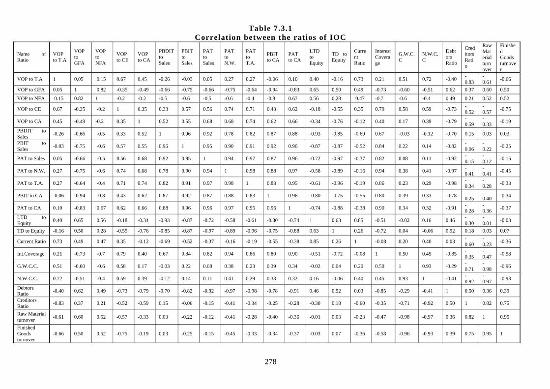
278
Table 7.3.1 Correlation between the ratios of IOC
nove
.66
50
52
.75
.19
03
.25
.15
.45
.33
.34
.37
.03
07
.36
.58
.96
.93
39
75
95
Name of Ratio
VOP to T.A
VOP to T.A 1
VOP to GFA 0.
VOP to NFA 0.
VOP to CE 0.
VOP to CA 0.
PBDIT to Sales -0
PBIT to Sales -0
PAT to Sales 0.
PAT to N.W. 0.
PAT to T.A. 0.
PBIT to CA -0
PAT to CA 0.
LTD to Equity 0.
TD to Equity -0
Current Ratio 0.
Int.Coverage 0.
G.W.C.C. 0.
N.W.C.C. 0.
Debtors Ratio -0
Creditors Ratio -0
Raw Material turnover -0
Finished Goods turnover
-0
VOP to GFA
VOP to NFA
VOP to CE
VOP to CA
PBDIT to Sales
PBIT to Sales
PAT to Sales
PAT to N.W.
PAT to T.A.
PBIT to CA
PAT to CA
LTD to Equity
TD to Equity
Current Ratio
Interest Coverage
G.W.C.C
N.W.C.C
Debtors Ratio
Creditors Ratio
Raw Material turnover
Finished Goods turr
0.05 0.15 0.67 0.45 -0.26 -0.03 0.05 0.27 0.27 -0.06 0.10 0.40 -0.16 0.73 0.21 0.51 0.72 -0.40 -0.83
-0.61 -0
05 1 0.82 -0.35 -0.49 -0.66 -0.75 -0.66 -0.75 -0.64 -0.94 -0.83 0.65 0.50 0.49 -0.73 -0.60 -0.51 0.62 0.37 0.60 0.
15 0.82 1 -0.2 -0.2 -0.5 -0.6 -0.5 -0.6 -0.4 -0.8 0.67 0.56 0.28 0.47 -0.7 -0.6 -0.4 0.49 0.21 0.52 0.
67 -0.35 -0.2 1 0.35 0.33 0.57 0.56 0.74 0.71 0.43 0.62 -0.18 -0.55 0.35 0.79 0.58 0.59 -0.73 -0.52
-0.57 -0
45 -0.49 -0.2 0.35 1 0.52 0.55 0.68 0.68 0.74 0.62 0.66 -0.34 -0.76 -0.12 0.40 0.17 0.39 -0.79 -0.59
-0.33 -0
.26 -0.66 -0.5 0.33 0.52 1 0.96 0.92 0.78 0.82 0.87 0.88 -0.93 -0.85 -0.69 0.67 -0.03 -0.12 -0.70 0.15 0.03 0.
.03 -0.75 -0.6 0.57 0.55 0.96 1 0.95 0.90 0.91 0.92 0.96 -0.87 -0.87 -0.52 0.84 0.22 0.14 -0.82 -0.06
-0.22 -0
05 -0.66 -0.5 0.56 0.68 0.92 0.95 1 0.94 0.97 0.87 0.96 -0.72 -0.97 -0.37 0.82 0.08 0.11 -0.92 -0.15
-0.12 -0
27 -0.75 -0.6 0.74 0.68 0.78 0.90 0.94 1 0.98 0.88 0.97 -0.58 -0.89 -0.16 0.94 0.38 0.41 -0.97 -0.41
-0.41 -0
27 -0.64 -0.4 0.71 0.74 0.82 0.91 0.97 0.98 1 0.83 0.95 -0.61 -0.96 -0.19 0.86 0.23 0.29 -0.98 -0.34
-0.28 -0
.06 -0.94 -0.8 0.43 0.62 0.87 0.92 0.87 0.88 0.83 1 0.96 -0.80 -0.75 -0.55 0.80 0.39 0.33 -0.78 -0.25
-0.40 -0
10 -0.83 0.67 0.62 0.66 0.88 0.96 0.96 0.97 0.95 0.96 1 -0.74 -0.88 -0.38 0.90 0.34 0.32 -0.91 -0.28
-0.36 -0
40 0.65 0.56 -0.18 -0.34 -0.93 -0.87 -0.72 -0.58 -0.61 -0.80 -0.74 1 0.63 0.85 -0.51 -0.02 0.16 0.46 -0.30
-0.01 -0
.16 0.50 0.28 -0.55 -0.76 -0.85 -0.87 -0.97 -0.89 -0.96 -0.75 -0.88 0.63 1 0.26 -0.72 0.04 -0.06 0.92 0.18 0.03 0.
73 0.49 0.47 0.35 -0.12 -0.69 -0.52 -0.37 -0.16 -0.19 -0.55 -0.38 0.85 0.26 1 -0.08 0.20 0.40 0.03 -0.60
-0.23 -0
21 -0.73 -0.7 0.79 0.40 0.67 0.84 0.82 0.94 0.86 0.80 0.90 -0.51 -0.72 -0.08 1 0.50 0.45 -0.85 -0.35
-0.47 -0
51 -0.60 -0.6 0.58 0.17 -0.03 0.22 0.08 0.38 0.23 0.39 0.34 -0.02 0.04 0.20 0.50 1 0.93 -0.29 -0.71
-0.98 -0
72 -0.51 -0.4 0.59 0.39 -0.12 0.14 0.11 0.41 0.29 0.33 0.32 0.16 -0.06 0.40 0.45 0.93 1 -0.41 -0.92
-0.97 -0
.40 0.62 0.49 -0.73 -0.79 -0.70 -0.82 -0.92 -0.97 -0.98 -0.78 -0.91 0.46 0.92 0.03 -0.85 -0.29 -0.41 1 0.50 0.36 0.
.83 0.37 0.21 -0.52 -0.59 0.15 -0.06 -0.15 -0.41 -0.34 -0.25 -0.28 -0.30 0.18 -0.60 -0.35 -0.71 -0.92 0.50 1 0.82 0.
.61 0.60 0.52 -0.57 -0.33 0.03 -0.22 -0.12 -0.41 -0.28 -0.40 -0.36 -0.01 0.03 -0.23 -0.47 -0.98 -0.97 0.36 0.82 1 0.
.66 0.50 0.52 -0.75 -0.19 0.03 -0.25 -0.15 -0.45 -0.33 -0.34 -0.37 -0.03 0.07 -0.36 -0.58 -0.96 -0.93 0.39 0.75 0.95 1

The table exhibits that value of production to total assets has very
minor correlation with gross assets but it has high positive relation with
value of production to capital employed. It has also positive high degree
relation with current ratio, net working capital cycle and creditors ratio.
Value of production to gross fixed assets has negative relationship with all
profitability ratios. Further, i t has also negative correlation with other key
ratios like creditors and debtors ratio and working capital cycle. It has
correlation with raw material turnover and with finished goods turnover
positively.
Profitability ratio has high degree negative correlation with debt to
equity ratios and debtors ratio. Debt to equity ratios, debtors ratio and
creditors ratio have almost negative relationship with other variables.
Current ratio has high degree positive relationship with profitability
ratio. It means profitability depends more upon current assets and liabilities.
Interest coverage ratio relates more with debtors ratio negatively. Both gross
working capital and net working capital have highly negative correlation with
debtors, creditors ratio as well as with finished goods turnover. Finished
goods turnover ratio has high degree positive correlation with finished goods
turnover.
7.3.2 Factor analysis of IOC
For further going analysis centroid factor of factor analysis method is
used. From correlation matrix, two centroid factors have been extracted here
in the table 7.3.2 and their communality and eigen values have been
calculated in the table 7.3.3.
279

Table 7.3.2
FACTOR LOADINGS OF IOC
Centroid Factor
Centroid Factor
Communality (h2)
Variables
A B (A2+B2)
Rank
VOP to T.A 0.4387 0.0026 0.1925 17 VOP to GFA -0.5682 -0.0034 0.3228 13 VOP to NFA 0.1815 0.0011 0.033 21 VOP to CE 0.8423 0.005 0.7094 8 VOP to CA 0.6535 0.0039 0.427 12 PBDIT to Sales 0.6753 0.004 0.456 11 PBIT to Sales 0.8223 0.0049 0.6762 9 PAT to Sales 0.8804 0.0052 0.7751 6 PAT to N.W. 0.953 0.0056 0.9082 2 PAT to T.A. 0.9494 0.0056 0.9013 3 PBIT to CA 0.7315 0.0043 0.5352 10 PAT to CA 0.8835 0.0052 0.7805 5 LTD to Equity -0.4516 -0.0027 0.204 16 TD to Equity -0.8695 -0.0051 0.756 7 Current Ratio 0.0118 0.0001 0.0001 22 Int. Coverage 0.8878 0.0053 0.7883 4 G.W.C.C. 0.3594 0.0021 0.1292 20 N.W.C.C. 0.4211 0.0025 0.1774 18 Debtors Ratio -0.9559 -0.0057 0.9138 1 Creditors Ratio -0.4611 -0.0027 0.2126 15 Raw Material turnover -0.3935 -0.0023 0.1549 19 Finished Goods turnover -0.4828 -0.0029 0.2331 14 Total 5.5088 0.0326 10.2865
Table 7.3.3
Centroid factors method of factor analysis for IOC
Factor loadings Centroid Factor Centroid Factor Variables
A B
Communality (h2)
Eigen value(Variance accounted for i.e.,common
variance) 5.51 0.03 5.54
Proportion of total variance 0.25 (25%) 0.002 (0.2%) 0.25 (25%)
Proportion of common variance
0.99 (99%) 0.006 (0.6%) 1.00 (100%)
Each communality in the table 7.3.3 represents the proportion of
variance in the corresponding row and is accounted for by the two factors A
280

and B . Here, total variance (variables) is 22.00 it means 22 ratios of various
variables have taken as variance. The eigen value or conman variance gives
the numerical value of that portion of the variance attributed to the factor in
the concerning column here, total value 22.00 is partitioned into 5.51 as
eigen value for factor A and 0.03 as eigen value for factor B and the total
5.54 as the sum of eigen values for these two factors. The corresponding
proportion of the total variance, 22.00, is shown in the next row. There we
can notice that 25% of the total variance is related to these two factors, i .e.
approximately 25% of the total variance is common variance whereas
remaining 75% of it is made up of portion unique to individual variables and
the techniques used to measure them. The last row shows that of the common
variance approximately 99% are accounted for by factor A and the other 1%
by factor B Thus it can be concluded that only one type of factors explain the
common variance.
From the table 7.3.2 it can be seen that only 6 variables are most
effective variables out of 22 variables in the unit which can be said loading
factor of unit, while other variables are independent factors for the unit. The
loading factors can be listed form the table 7.3.2. These are profit after tax to
net worth, profit after tax to current assets, debtors ratio, profit after tax to
sales, profit after tax to capital employed, interest coverage. So, company has
to concentrate more on these variables to perform better and to improve its
financial position. Further, giving rank to most loading factors net profit to
net worth and net profit to total assets as well as debtors ratio are getting
highest rank. They are most distressing factors for the company. They need
more attention for better performance.
7.4.1 Correlation matrix of MRP
The table 7.4.1 shows the correlation matrix of the 22 ratios of various
variables of the firm MRP. Ratios have been calculated from the data for the
period of study 1998-2003.
281

282

283
Table 7.4.1 Correlation between the ratios of MRP
Finished Goods
turnover
0.29 0.15
082
-0.20
-0.37 0.64
0.73
0.80
0.49
0.64
0.74
0.59
-0.50
0.53 0.81
0.91
-0.49 0.12
-0.71
-0.62
0.11
1
Name of Ratio
VOP to T.A
VOP to T.A 1
VOP to GFA 0.58
VOP to NFA 0.63
VOP to CE 0.98
VOP to CA 0.99
PBDIT to Sales
-0.66
PBIT to Sales
-0.64
PAT to Sales -0.57
PAT to N.W. -0.78
PAT to T.A. -0.83
PBIT to CA -0.66
PAT to CA -0.86
LTD to Equity
0.15
TD to Equity 0.21
Current Ratio
-0.33
Int. Coverage
-0.50
G.W.C.C. -0.41
N.W.C.C. -0.63
Debtors Ratio
0.66
Creditors Ratio
-0.12 -
Raw Material turnover
0.61
Finished Goods
turnover -0.29
VOP
to GFA
VOP to
NFA
VOP to CE
VOP to- CA
PBDIT to
Sales
PBIT to
Sales
PAT to
Sales
PAT to
N.W.
PAT to
T.A.
PBIT to CA
PAT to CA
LTD to
Equity
TD to Equity
Current
Ratio
Interest Covera
ge
G.W.C.C
N.W.C.C
Debtors Ratio
Creditors Ratio
Raw Materia
l turnove
r
0.58 0.63 0.98 0.99 -0.66 -0.64 -0.57 -0.78 -0.83 -0.66 -0.86 0.15 0.21 -0.33 -0.50 -0.41 -0.63 0.66 -0.12 0.61 -
1 0.99 0.48 0.54 -0.45 0.37 -0.20 -0.14 -0.29 -0.32 -0.27 -0.44 -0.40 0.36 -0.06 -0.85 -0.27 -0.07 -0.83 0.82
0.99 1 0.53 0.60 -0.50 -0.42 -0.25 -0.19 -0.34 -0.38 -0.32 -0.42 -0.38 0.29 -0.13 -0.82 -0.29 -0.002 -0.78 0.81 0.
0.48 0.53 1 0.96 -0.51 -0.50 -0.45 -0.77 -0.76 -0.52 -0.81 0.15 0.21 -0.36 -0.38 -0.34 -0.58 0.62 -0.07 0.49
0.54 0.60 0.96 1 -0.73 -0.71 -0.65 -0.81 -0.86 -0.73 -0.89 0.20 0.26 -0.36 -0.58 -0.37 -0.68 0.73 -0.06 0.61
-0.45 -0.50 -0.51 -0.73 1 0.96 0.88 0.62 0.78 0.98 0.74 -0.21 -0.27 0.24 0.88 0.29 0.67 -0.74 -0.03 -0.65
0.37 -0.42 -0.50 -0.71 0.96 1 0.97 0.74 0.88 0.99 0.83 -0.44 -0.49 0.37 0.89 0.19 0.67 -0.80 -0.13 -0.58
-0.20 -0.25 -0.45 -0.65 0.88 0.97 1 0.79 0.90 0.95 0.86 -0.61 -0.66 0.49 0.90 0.03 0.64 -0.86 -0.30 -0.45
-0.14 -0.19 -0.77 -0.81 0.62 0.74 0.79 1 0.96 0.72 0.97 -0.72 -0.77 0.52 0.60 0.10 0.77 -0.89 -0.30 -0.42
-0.29 -0.34 -0.76 -0.86 0.78 0.88 0.90 0.96 1 0.86 0.99 -0.61 -0.66 0.55 0.75 0.13 0.72 -0.90 -0.23 -0.49
-0.32 -0.38 -0.52 -0.73 0.98 0.99 0.95 0.72 0.86 1 0.82 -0.40 -0.45 0.39 0.93 0.15 0.68 -0.84 -0.18 -0.55
-0.27 -0.32 -0.81 -0.89 0.74 0.83 0.86 0.97 0.99 0.82 1 -0.61 -0.66 0.56 0.71 0.13 0.73 -0.91 -0.24 -0.47
-0.44 -0.42 0.15 0.20 -0.21 -0.44 -0.61 -0.72 -0.61 -0.40 -0.61 1 0.99 -0.54 -0.40 0.36 -0.46 0.68 0.65 -0.07
-0.40 -0.38 0.21 0.26 -0.27 -0.49 -0.66 -0.77 -0.66 -0.45 -0.66 0.99 1 -0.57 -0.45 0.34 -0.49 0.73 0.65 -0.04 -
0.36 0.29 -0.36 -0.36 0.24 0.37 0.49 0.52 0.55 0.39 0.56 -0.54 -0.57 1 0.61 -0.70 -0.05 -0.64 -0.76 0.43
-0.06 -0.13 -0.38 -0.58 0.88 0.89 0.90 0.60 0.75 0.93 0.71 -0.40 -0.45 0.61 1 -0.19 0.45 -0.84 -0.45 -0.23
-0.85 -0.82 -0.34 -0.37 0.29 0.19 0.03 0.10 0.13 0.15 0.13 0.36 0.34 -0.70 -0.19 1 0.48 0.15 0.88 -0.90
-0.27 -0.29 -0.58 -0.68 0.67 0.67 0.64 0.77 0.72 0.68 0.73 -0.46 -0.49 -0.05 0.45 0.48 1 -0.72 0.01 -0.74
-0.07 -0.002 0.62 0.73 -0.74 -0.80 -0.86 -0.89 -0.90 -0.84 -0.91 0.68 0.73 -0.64 -0.84 0.15 -0.72 1 0.55 0.26
0.83 -0.78 -0.07 -0.06 -0.03 -0.13 -0.30 -0.30 -0.23 -0.18 -0.24 0.65 0.65 -0.76 -0.45 0.88 0.01 0.55 1 -0.63
0.82 0.81 0.49 0.61 -0.65 -0.58 -0.45 -0.42 -0.49 -0.55 -0.47 -0.07 -0.04 0.43 -0.23 -0.90 -0.74 0.26 -0.63 1
0.15 0.082 -0.20 -0.37 0.64 0.73 0.80 0.49 0.64 0.74 0.59 -0.50 -0.53 0.81 0.91 -0.49 0.12 -0.71 -0.62 0.11

The 7.4.1 table exhibits that value of production correlates highly with
positive relation with production to capital employed and current assets i t
also correlates positively with high degree with raw material turnover. Value
of production to gross fixed assets correlates highly with production to net
fixed assets and raw material turnover but correlates negatively with
creditors ratio. Value of production to gross fixed assets correlates highly
with production to net fixed assets and raw material turnover but correlates
negatively with creditors ratio. Value of production to net fixed assets has
positive effect on raw material turnover. All the production to assets ratios
have negative correlation with profitability ratios.
PBDIT to sales ratio has high degree positive correlation with Profit
after tax to sales and interest coverage ratio. PBIT to sales with Profit after
tax to sales and Profir after taxto sales with other profitability ratios
correlates positively with high degree. But the all profitability ratios have
negative relationship with debt to equity ratio as well as creditors and
debtors ratio.
Long term debt to equity has very close relation with total debt to
equity. Further, i t has positive relation with debtors and creditors ratio, but
for all other variables it has negative relationship. Total debt to equity and
current ratio have high degree correlation only with debtors ratio. Interest
coverage correlates highly with finished good turnover. Gross w0orking
capital cycle has positive high degree correlation with creditors ratio and
negative high degree correlation with raw material turnover while, Net
working capital cycle have high degree negative relation with debtors ratio
and raw material turnover.
7.4.2 Factor analysis of MRP
For further going analysis centroid factor of factor analysis method is
used. From correlation matrix, two centroid factors have been extracted here
284

in the table 7.4.2 and their communality and eigen values have been
calculated in the table 7.4.3.
Table 7.4.2
FACTOR LOADINGS OF MRP
Centroid Factor
Centroid Factor
Communality (h2)
Variables
A B (A2+B2)
Rank
VOP to T.A -0.3085 0 0.0952 17 VOP to GFA 0.1469 0 0.0216 21 VOP to NFA -0.0609 0 0.0037 22 VOP to CE -0.1742 0 0.0303 20 VOP to CA -0.4009 0 0.1607 16 PBDIT to Sales 0.8249 0 0.6805 6 PBIT to Sales 1.0243 0 1.0492 1 PAT to Sales 0.8836 0 0.7807 2 PAT to N.W. 0.5226 0 0.2731 10 PAT to T.A. 0.6695 0 0.4482 8 PBIT to CA 0.8773 0 0.7697 3 PAT to CA 0.6066 0 0.368 9 LTD to Equity -0.4722 0 0.223 13 TD to Equity -0.51 0 0.2601 11 Current Ratio 0.4848 0 0.235 12 Int. Coverage 0.8277 0 0.6851 5 G.W.C.C. -0.1763 0 0.0311 19 N.W.C.C. 0.4261 0 0.1816 14 Debtors Ratio -0.7434 0 0.5526 7 Creditors Ratio -0.4177 0 0.1745 15 Raw Material turnover -0.2267 0 0.0514 18 Finished Goods turnover 0.861 0 0.7413 4 Total 4.6645 0 7.8166
Table 7.4.3
Centroid factors method of factor analysis for MRP
Factor loadings Centroid Factor Centroid Factor Variables
A B
Communality (h2)
Eigen value(Variance accounted for i.e.,common
variance) 4.76 0 4.76
Proportion of total variance 0.22 (22%) 0 0.22 (22%)
Proportion of common variance
1.00 (100%) 0 1.00 (100%)
285

Each communality in the table 7.4.3 represents the proportion of
variance in the corresponding row and is accounted for by the two factors A
and B . Here, total variance (variables) is 22.00 it means 22 ratios of various
variables have taken as variance. The eigen value or conman variance gives
the numerical value of that portion of the variance attributed to the factor in
the concerning column here, total value 22.00 is partitioned into 4.76 as
eigen value for factor A and zero value as eigen value for factor B and the
total 4.76 as the sum of eigen values for these two factors. The corresponding
proportion of the total variance, 22.00, is shown in the next row. There we
can notice that 22% of the total variance is related to these two factors, i .e.
approximately 22% of the total variance is common variance whereas
remaining 78% of it is made up of portion unique to individual variables and
the techniques used to measure them. The last row shows that of the common
variance all (i .e.100%) are accounted for by factor A and no variables are
accounted by factor B Thus it can be concluded that only one type of factors
explain the common variance.
From the table 7.4.3 it can be seen that only 5 variables are most
effective variables out of 22 variables in the unit which can be said loading
factor of unit, while other variables are independent factors for the unit. The
loading factors can be listed form the table 7.4.2. These are finished goods
profit before interest tax to sales, profit after tax to sales, profit before
interest tax to current assets, profit before interest tax to sales, interest
coverage. So, company has to concentrate more on these variables to perform
better and to improve its financial position. Further, giving rank to most
loading factors profitability to current assets and sales are getting highest
rank. They are most distressing factors for the company. They need more
attention for better performance.
7.5.1 Correlation matrix of BRP
The table 7.5.1 shows the correlation matrix of the 22 ratios of various
variables of the firm BRP. Ratios have been calculated from the data for the
286

287
period of study 1998-2003. From the table, relation between the various
ratios and the degree of relation between them can be found out here.

288
Table 7.5.1 Correlation between the ratios of BRP
Finished Goods
turnover
78
86
84
93
51
-0.14
-0.15
-0.29
-0.02
-0.20
08 -
0.17 -
0.69 94 -
0.84 13 -
0.73 -
0.72
71
63
-0.72
1
Name of Ratio
VOP to T.A
VOP to T.A 1
VOP to GFA 0.
VOP to NFA 0.
VOP to CE 0.
VOP to CA 0.
PBDIT to Sales
0.
PBIT to Sales 0.
PAT to Sales 0.
PAT to N.W. 0.
PAT to T.A. 0.
PBIT to CA 0.
PAT to CA 0.
LTD to Equity
-0
TD to Equity 0.
Current Ratio -0
Int. Coverage 0.
G.W.C.C. -0
N.W.C.C. -0
Debtors Ratio
0.
Creditors Ratio
0.
Raw Material turnover -0
Finished Goods
turnover 0.
VOP to
GFA
VOP to
NFA
VOP to CE
VOP to- CA
PBDIT to
Sales
PBIT to
Sales
PAT to
Sales
PAT to
N.W.
PAT to
T.A.
PBIT to CA
PAT to CA
LTD to
Equity
TD to Equity
Current
Ratio
Interest Covera
ge
G.W.C.C
N.W.C.C
Debtors Ratio
Creditors Rati
o
Raw Materia
l turnove
r
0.96 0.65 0.82 0.69 0.09 0.10 0.01 0.26 0.11 0.34 0.18 -0.85 0.56 -0.51 0.29 -0.96 -0.69 0.69 0.41 -0.42 0.96 1 0.83 0.94 0.50 0.22 0.23 0.11 0.38 0.20 0.47 0.27 -0.73 0.67 -0.53 0.43 -0.91 -0.77 -0.51 0.61 -0.48 0.65 0.83 1 0.95 0.06 0.38 0.36 0.21 0.45 0.29 0.53 0.30 -0.31 0.78 -0.51 0.57 -0.62 -0.79 0.94 0.90 -0.49 0.82 0.94 0.95 1 0.32 0.20 0.19 0.05 0.32 0.14 0.42 0.18 -0.58 0.83 -0.64 0.42 -0.76 -0.78 0.89 0.76 -0.61 0.69 0.50 0.06 0.32 1 -0.51 -0.49 -0.51 -0.40 -0.46 -0.35 -0.43 -0.84 0.37 -0.54 -0.29 -0.72 -0.40 0.02 -
0.01 -0.24 0.
09 0.22 0.38 0.20 -0.51 1 0.99 0.98 0.97 0.99 0.95 0.96 0.40 -0.28 0.56 0.93 -0.15 -0.34 0.58 0.54 0.45
10 0.23 0.36 0.19 -0.49 0.99 1 0.99 0.98 0.99 0.96 0.97 0.38 -0.30 0.58 0.93 -0.16 -0.32 0.57 0.51 0.45
01 0.11 0.21 0.05 -0.51 0.98 0.99 1 0.95 0.99 0.91 0.97 0.45 -0.44 0.69 0.88 -0.08 -0.22 0.45 0.40 0.56
26 0.38 0.45 0.32 -0.40 0.97 0.98 0.95 1 0.98 0.99 0.99 0.21 -0.21 0.49 0.93 -0.29 -0.37 0.68 0.53 0.33
11 0.20 0.29 0.14 -0.46 0.99 0.99 0.99 0.98 1 0.95 0.98 0.36 -0.37 0.63 0.91 -0.17 -0.29 0.53 0.45 0.51
34 0.47 0.53 0.42 -0.35 0.95 0.96 0.91 0.99 0.95 1 0.97 0.13 -0.11 0.39 0.92 -0.35 -0.42 0.75 0.58 0.23 0.18 0.27 0.30 0.18 -0.43 0.96 0.97 0.97 0.99 0.98 0.97 1 0.26 -0.35 0.60 0.87 -0.20 -0.24 0.56 0.39 0.41
.85 -0.73 -0.31 -0.58 -0.84 0.40 0.38 0.45 0.21 0.36 0.13 0.26 1 -0.54 0.65 0.24 0.75 0.33 -0.29 0.03 0.60
56 0.67 0.78 0.83 0.37 -0.28 -0.30 -0.44 -0.21 -0.37 -0.11 -0.35 -0.54 1 -0.92 -0.04 -0.49 -0.58 0.55 0.58 -0.81 0..51 -0.53 -0.51 -0.64 -0.54 0.56 0.58 0.69 0.49 0.63 0.39 0.60 0.65 -0.92 1 0.38 0.40 0.35 -0.25 -
0.26 0.86
29 0.43 0.57 0.42 -0.29 0.93 0.93 0.88 0.93 0.91 0.92 0.87 0.24 -0.04 0.38 1 -0.40 -0.63 0.75 0.75 0.38 0..96 -0.91 -0.62 -0.76 -0.72 -0.15 -0.16 -0.08 -0.29 -0.17 -0.35 -0.20 0.75 -0.49 0.40 -0.40 1 0.82 -0.68 -
0.49 0.20
.69 -0.77 -0.79 -0.78 -0.40 -0.34 -0.32 -0.22 -0.37 -0.29 -0.42 -0.24 0.33 -0.58 0.35 -0.63 0.82 1 -0.78 -0.85 0.06
69 0.85 0.94 0.89 0.02 0.58 0.57 0.45 0.68 0.53 0.75 0.56 -0.29 0.55 -0.25 0.75 -0.68 -0.78 1 0.86 -0.29 0.
41 0.61 0.90 0.76 -0.01 0.54 0.51 0.40 0.53 0.45 0.58 0.39 0.03 0.58 -0.26 0.75 -0.49 -0.85 0.86 1 -0.13 0.
.42 -0.48 -0.49 -0.61 -0.24 0.45 0.45 0.56 0.33 0.51 0.23 0.41 0.60 -0.81 0.86 0.38 0.20 0.06 -0.29 -0.13 1
78 0.86 0.84 0.93 0.51 -0.14 -0.15 -0.29 -0.02 -0.20 0.08 -0.17 -0.69 0.94 -0.84 0.13 -0.73 -0.72 0.71 0.63 -0.72

The 7.5.1 table exhibits that value of production to total assets has
high relationship with value of production to gross fixed assets. so, both
ratios have same relationship with other ratios. They are positively correlates
with other ratios of value of production ratio. They have very minor
relationship with profitability ratios. The value of production to total assets
ratio has negative relationship with working capital cycle. The value of
production to net fixed assets, value of production to capital employed and
value of production to current assets negatively relates with working capital
cycle ratios. Value of production to current assets has negative correlation
with almost all ratios.
All the profitability ratios are interred co-related highly with each
other. They have negative relationship with working capital cycle, finished
goods turnover and long term debt to equity ratio. Long term debt to equity
has negative correlation with total debt to equity, debtors ratios and finished
goods turnover ratio, while it has positive high degree correlation with gross
working capital cycle. Total debt to equity has high degree negative
correlation with current ratio and high degree positive correlation with
finished goods turnover. Interest coverage ratio highly correlates with
debtors and creditors ratio, while working capital cycle has negative
correlation with debtors and creditors ratio. Raw material turnover ratio
correlates negatively with finished goods turnover ratio.
7.5.2 Factor analysis of BRP
For further going analysis centroid factor of factor analysis method is
used. From correlation matrix, two centroid factors have been extracted here
in the table 7.5.2 and their communality and eigen values have been
calculated in the table 7.5.3.
289

Table 7.5.2
FACTOR LOADINGS OF BRP
Centroid Factor
Centroid Factor
Communality (h2)
Variables
A B (A2+B2)
Rank
VOP to T.A 0.4245 0 0.1802 17 VOP to GFA 0.575 0 0.3306 13 VOP to NFA 0.6889 0 0.4746 11 VOP to CE 0.5636 0 0.3176 14 VOP to CA -0.526 0 0.2767 15
PBDIT to Sales 0.9195 0 0.8455 4 PBIT to Sales 0.9186 0 0.8438 5 PAT to Sales 0.8525 0 0.7268 8 PAT to N.W. 0.9553 0 0.9126 3 PAT to T.A. 0.896 0 0.8028 6 PBIT to CA 0.9732 0 0.9471 2 PAT to CA 0.8913 0 0.7944 7
LTD to Equity 0.0904 0 0.0082 21 TD to Equity 0.0791 0 0.0063 22 Current Ratio 0.2428 0 0.059 19 Int. Coverage 0.9741 0 0.9489 1
G.W.C.C. -0.4696 0 0.2205 16 N.W.C.C. -0.624 0 0.3894 12
Debtors Ratio 0.7275 0 0.5293 10 Creditors Ratio 0.7708 0 0.5941 9 Raw Material
turnover 0.1741 0 0.0303 20 Finished Goods
turnover 0.2579 0 0.0665 18 Total 10.3555 0 10.3051
Table 7.5.3
Centroid factors method of factor analysis for BRP
Factor Loadings Variables Centroid Factor A Centroid Factor B
Communtality (h2)
Eigen Value (variance Accunted for i.e.common variance)
10.6253 0 10.6253
Proportion of Total Variance 0.48 (48%) 0 0.48 (48%)
Proportion of Common Variance
1.00 (100%) 0 1.00 (100%)
Each communality in the table 7.5.3 represents the proportion of
variance in the corresponding row and is accounted for by the two factors A
290

291
and B . Here, total variance (variables) is 22.00 it means 22 ratios of various
variables have taken as variance. The eigen value or conman variance gives
the numerical value of that portion of the variance attributed to the factor in
the concerning column here, total value 22.00 is partitioned into 10.6253 as
eigen value for factor A and zero as eigen value for factor B and the total
10.6253 as the sum of eigen values for these two factors. The corresponding
proportion of the total variance, 22.00, is shown in the next row. There we
can notice that 48% of the total variance is related to these two factors, i .e.
approximately 48% of the total variance is common variance whereas
remaining 52% of it is made up of portion unique to individual variables and
the techniques used to measure them. The last row shows that of the common
variance approximately 100% are accounted for by factor A and no variables
are accounted for by factor B. Thus it can be concluded that only one type of
factors explain the common variance.
From the table 7.5.3 it can be seen that only 10 variables are most
effective variables out of 22 variables in the unit which can be said loading
factor of unit, while other variables are independent factors for the unit. The
loading factors can be listed form the table 7.5.2. These are interest
coverage, profit before depreciation, interest and taxes to sales, profit before
interest and tax to sales, profit after tax to sales, profit after sales to total
assets, profit after tax to capital employee, debtors ratio, creditors ratio,
profit before interest and tax to capital employee, profit after tax to net
worth. So, company has to concentrate more on these variables to perform
better and to improve its financial position. Further, giving rank to the
loading factors, interest coverage, profitability to current assets and net
profit to net worth are getting highest rank. So they are most distressing
factors for the unit . Company should give more attention to these factors.
7.6.1 Correlation matrix of KRL
The table 7.6.1 shows the correlation matrix of the 22 ratios of various
variables of the firm KRL. Ratios have been calculated from the data for the

period of study 1998-2003. . From the table, relation between the various
ratios and the degree of relation between them can be found out here.
292

293
Table 7.6.1 Correlation between the Ratios of KRL
Finished Goods
turnover
-0.43 0.36 0.40
02 -
0.62
0.29
0.32
0.44 0.32 0.09 0.21 0.37
-0.56
-0.90
-0.72
0.38
-0.96
-0.90
-0.76
57
-0.57
1
Name of Ratio
VOP to T.A
VOP to T.A
VOP to GFA 0.VOP to NFA 0.VOP to CE 0.
VOP to CA 0.
PBDIT to Sales 0.
PBIT to Sales 0.
PAT to Sales -0PAT to N.W. 0.PAT to T.A. 0.PBIT to CA 0.PAT to CA 0.
LTD to Equity -0
TD to Equity 0.
Current Ratio 0.
Int. Coverage 0.
G.W.C.C. 0.
N.W.C.C. 0.
Debtors Ratio 0.
Creditors Ratio -0
Raw Material turnover
0.
Finished Goods
turnover -0
VOP to
GFA
VOP to
NFA
VOP to CE
VOP to- CA
PBDIT to
Sales
PBIT to
Sales
PAT to
Sales
PAT to
N.W.
PAT to
T.A.
PBIT to CA
PAT to CA
LTD to
Equity
TD to Equity
Current
Ratio
Interest
Coverag
e
G.W.C.C
N.W.C.C
Debtors Ratio
Creditors Ratio
Raw Materia
l turnove
r
1 0.45 0.46 0.87 0.95 0.06 0.07 -0.002 0.40 0.65 0.52 0.39 -0.49 0.38 0.49 0.07 0.50 0.72 0.87 -0.76 0.97
45 1 0.96 0.78 0.17 0.45 0.53 0.62 0.78 0.77 0.67 0.77 -0.74 -0.47 -0.54 0.68 -0.41 -0.16 0.04 -0.20 0.33 46 0.96 1 0.76 0.19 0.67 0.72 0.77 0.92 0.90 0.85 0.92 -0.80 -0.57 -0.47 0.81 -0.39 -0.22 0.08 -0.04 0.38 87 0.78 0.76 1 0.70 0.19 0.23 0.23 0.61 0.76 0.64 0.62 -0.80 -0.03 0.07 0.31 0.03 0.33 0.54 -0.59 0.76 0.
95 0.17 0.19 0.70 1 -0.07 -0.08 -0.19 0.19 0.47 0.35 0.18 -0.28 0.59 0.72 -0.13 0.70 0.86 0.96 -0.76 0.97
06 0.45 0.67 0.19 -0.07 1 0.99 0.95 0.88 0.76 0.86 0.87 -0.37 -0.64 -0.31 0.90 -0.23 -0.41 -0.02 0.49 0.15
07 0.53 0.72 0.23 -0.08 0.99 1 0.98 0.91 0.79 0.87 0.90 -0.41 -0.66 -0.37 0.94 -0.27 -0.42 -0.04 0.48 0.15
.002 0.62 0.77 0.23 -0.19 0.95 0.98 1 0.91 0.76 0.82 0.90 -0.46 -0.74 -0.53 0.98 -0.40 -0.52 -0.17 0.51 0.04 40 0.78 0.92 0.61 0.19 0.88 0.91 0.91 1 0.95 0.97 0.99 -0.70 -0.58 -0.32 0.91 -0.26 -0.24 0.15 0.17 0.40 65 0.77 0.90 0.76 0.47 0.76 0.79 0.76 0.95 1 0.97 0.95 -0.70 -0.34 -0.09 0.78 -0.02 0.04 0.42 -0.09 0.65 52 0.67 0.85 0.64 0.35 0.86 0.87 0.82 0.97 0.97 1 0.97 -0.69 -0.47 -0.10 0.81 -0.11 -0.11 0.31 0.08 0.54 39 0.77 0.92 0.62 0.18 0.87 0.90 0.90 0.99 0.95 0.97 1 -0.74 -0.61 -0.31 0.90 -0.29 -0.27 0.13 0.19 0.38
.49 -0.74 -0.80 -0.80 -0.28 -0.37 -0.41 -0.46 -0.70 -0.70 -0.69 -0.74 1 0.50 0.21 -0.49 0.43 0.21 -0.09 0.06 -0.34
38 -0.47 -0.57 -0.03 0.59 -0.64 -0.66 -0.74 -0.58 -0.34 -0.47 -0.61 0.50 1 0.77 -0.65 0.89 0.91 0.68 -0.64 0.45
49 -0.54 -0.47 0.07 0.72 -0.31 -0.37 -0.53 -0.32 -0.09 -0.10 -0.31 0.21 0.77 1 -0.51 0.86 0.78 0.79 -0.43 0.58
07 0.68 0.81 0.31 -0.13 0.90 0.94 0.98 0.91 0.78 0.81 0.90 -0.49 -0.65 -0.51 1 -0.34 -0.44 -0.09 0.45 0.10
50 -0.41 -0.39 0.03 0.70 -0.23 -0.27 -0.40 -0.26 -0.02 -0.11 -0.29 0.43 0.89 0.86 -0.34 1 0.90 0.85 -0.49 0.64
72 -0.16 -0.22 0.33 0.86 -0.41 -0.42 -0.52 -0.24 0.04 -0.11 -0.27 0.21 0.91 0.78 -0.44 0.90 1 0.90 -0.82 0.77
87 0.04 0.08 0.54 0.96 -0.02 -0.04 -0.17 0.15 0.42 0.31 0.13 -0.09 0.68 0.79 -0.09 0.85 0.90 1 -0.66 0.94
.76 -0.20 -0.04 -0.59 -0.76 0.49 0.48 0.51 0.17 -0.09 0.08 0.19 0.06 -0.64 -0.43 0.45 -0.49 -0.82 -0.66 1 -0.69 0.
97 0.33 0.38 0.76 0.97 0.15 0.15 0.04 0.40 0.65 0.54 0.38 -0.34 0.45 0.58 0.10 0.64 0.77 0.94 -0.69 1
.43 0.36 0.40 0.02 -0.62 0.29 0.32 0.44 0.32 0.09 0.21 0.37 -0.56 -0.90 -0.72 0.38 -0.96 -0.90 -0.76 0.57 -0.57

The 7.6.1 table indicates that value of production to total assets has
high degree positive correlation with value of production to current assets. It
means the total asset has very close relation with current assets than fixed
assets. It has also highly positively correlation with debtors ratio and raw
material turnover.
Value of production to gross fixed assets has high degree positive
correlation with value of production to net fixed assets as well as value of
production to capital employed. Further, i t has high positive correlation with
all profitability ratios. It has negative relation with long term debt to equity
ratio. Value of production to net fixed assets has the same type of correlation
with the other ratios as value of production to gross fixed assets has relation
with other ratios. .
Value of production to current assets highly and positively correlates
only with debtors ratio and raw material turnover. All profitability ratios
interrelates high degree positively with each other. However, they have high
degree negative relation with both total debt to equity and long term debt to
equity ratio. They have high degree correlation with interest coverage ratio
also. Total debt to equity ratio and current ratio has degree high correlation
with working capital cycle.
Net working capital cycle have high relation negatively with finished
good turnover ratio and positively with finished good turnover ratio and
positively with debtors ratio. And at last debtors ratio has positive high
correlation with finished goods turnover.
7.6.2 Factor analysis of KRL
For further going analysis centroid factor of factor analysis method is
used. From correlation matrix, two centroid factors have been extracted here
in the table 7.6.2 and their communality and eigen values have been
calculated in the table 7.6.3.
294

Table 7.6.2
FACTOR LOADINGS OF KRL
Centroid Factor
Centroid Factor
Communality (h2)
Variables
A B (A2+B2)
Rank
VOP to T.A 0.7496 -0.0044 0.5619 7 VOP to GFA 0.63 -0.0037 0.3969 14 VOP to NFA 0.7645 -0.0045 0.5845 6 VOP to CE 0.7396 -0.0043 0.547 8 VOP to CA 0.6328 -0.0037 0.4004 13
PBDIT to Sales 0.6871 -0.004 0.4721 10 PBIT to Sales 0.7028 -0.0041 0.4939 9 PAT to Sales 0.6354 -0.0037 0.4037 12 PAT to N.W. 0.8621 -0.005 0.7432 3 PAT to T.A. 0.9644 -0.0056 0.9301 1 PBIT to CA 0.9174 -0.0053 0.8416 2 PAT to CA 0.8483 -0.0049 0.7196 4
LTD to Equity -0.5757 0.0034 0.3314 16 TD to Equity -0.1041 0.0006 0.0108 22 Current Ratio 0.1446 -0.0008 0.0209 21 Int. Coverage 0.6787 -0.004 0.4606 11
G.W.C.C. 0.2422 -0.0014 0.0587 18 N.W.C.C. 0.268 -0.0016 0.0718 17
Debtors Ratio 0.6291 -0.0037 0.3958 15 Creditors Ratio -0.1999 0.0012 0.04 19 Raw Material
turnover 0.792 -0.0046 0.6273 5 Finished Goods
turnover -0.152 0.0009 0.0231 20 Total 10.8569 -0.0632 9.1354
Table 7.6.3
Centroid factors method of factor analysis for KRL
Factor loadings Centroid Factor Centroid Factor Variables
A B
Communality (h2)
Eigen value(Variance accounted for i.e.,common
variance) 10.86 0.06 10.92
Proportion of total variance 0.49 (49%) 0.002 0.50 (50%)
Proportion of common variance
0.99 (99%) 0.006 (1%) 1.00 (100%)
Each communality in the table 7.6.3 represents the proportion of
variance in the corresponding row and is accounted for by the two factors A
295
and B . Here, total variance (variables) is 22.00 it means 22 ratios of various
variables have taken as variance. The eigen value or conman variance gives
the numerical value of that portion of the variance attributed to the factor in
the concerning column here, total value 22.00 is partitioned into 10.86 as
eigen value for factor A and 0.06 as eigen value for factor B and the total
10.92 as the sum of eigen values for these two factors. The corresponding
proportion of the total variance, 22.00, is shown in the next row. There we
can notice that 50% of the total variance is related to these two factors, i .e.
approximately 50% of the total variance is common variance whereas
remaining 50% of it is made up of portion unique to individual variables and
the techniques used to measure them. The last row shows that of the common
variance approximately 99% are accounted for by factor A and the other 1%
by factor B Thus it can be concluded that only one type of factors explain the
common variance.
From the table 7.6.3 it can be seen that only 11 variables are most
effective variables out of 22 variables in the unit which can be said loading
factor of unit, while other variables are independent factors for the unit. The
loading factors can be listed form the table 7.6.2. These are profit after tax to
total assets, profit before interest tax to current assets, profit after tax to net
worth, profit after tax to current assets, raw material turnover, value of
production to total assets, value of production to net fixed assets, value of
production to capital employed, value of production to current assets, profit
before debtors interest tax to sales, profit before interest tax to sales. So,
company has to concentrate more on these variables to perform better and to
improve its financial position. Further, giving rank to most loading factors
net profit in relation to total assets and net worth as well as profitability to
current assets are getting highest rank. They are most distressing factors for
the company. They need more attention for better performance.
296

297
Table 7.7.1 Correlation between the Ratios of CPCL
Finished Goods
turnover 0.81
0.59
50
0.68
71 -
0.87 -
0.84 -
0.84 -
0.59 -
0.22 -
0.66 -
0.64
0.07
-0.56
0.90
-0.33
-0.75 0.75
-0.07
-0.79
0.56
1
Name of Ratio
VOP to T.A
VOP to GFA
VOP to NFA
VOP to CE
VOP to CA PBDIT to
Sales PBIT to
Sales
PAT to Sales
PAT to N.W.
PAT to T.A.
PBIT to CA
PAT to CA
LTD to Equity
TD to Equity
Current Ratio Int.
Coverage
G.W.C.C.
N.W.C.C. Debtors
Ratio Creditors
Ratio Raw
Material turnover Finished Goods
turnover
VOP to T.A
VOP to
GFA
VOP to
NFA
VOP to CE
VOP to- CA
PBDIT to
Sales
PBIT to
Sales
PAT to
Sales
PAT to
N.W.
PAT to
T.A.
PBIT to CA
PAT to CA
LTD to
Equity
TD to Equity
Current Rati
o
Interest Covera
ge
G.W.C.C
N.W.C.C
Debtors Rati
o
Creditors Ratio
Raw Materia
l turnove
r
1 0.84 0.80 0.93 0.98 -0.85 -0.75 -0.77 -0.21 0.28 -0.34 -0.36 0.55 -0.16 0.68 0.09 -0.43 0.96 0.39 -0.96 0.73
0.84 1 0.99 0.98 0.84 -0.73 -0.47 -0.48 0.18 0.59 0.01 0.06 0.42 0.004 0.50 0.52 -0.54 0.84 0.66 -0.89 0.90
0.80 0.99 1 0.96 0.82 -0.66 -0.39 -0.40 0.28 0.66 0.12 0.16 0.50 0.14 0.38 0.61 -0.49 0.81 0.68 -0.86 0.93 0.
0.93 0.98 0.96 1 0.93 -0.78 -0.58 -0.59 0.06 0.52 -0.09 -0.07 0.52 -0.03 0.56 0.40 -0.49 0.92 0.60 -0.95 0.87
0.98 0.84 0.82 0.93 1 -0.81 -0.70 -0.73 -0.12 0.37 -0.26 -0.30 0.69 0.01 0.57 0.18 -0.33 0.97 0.43 -0.95 0.74 0.
-0.85 -0.73 -0.66 -0.78 -0.81 1 0.94 0.93 0.52 0.89 0.66 0.61 -0.32 0.22 -0.89 0.16 0.65 -0.91 -
0.04 0.92 -0.63
-0.75 -0.47 -0.39 -0.58 -0.70 0.94 1 0.99 0.76 0.35 0.86 0.84 -0.27 0.31 -0.91 0.46 0.48 -0.81 0.18 0.78 -0.35
-0.77 -0.48 -0.40 -0.59 -0.73 0.93 0.99 1 0.74 0.32 0.84 0.84 -0.31 0.30 -0.90 0.45 0.46 -0.83 0.16 0.79 -0.35
-0.21 0.18 0.28 0.06 -0.12 0.52 0.76 0.74 1 0.87 0.98 0.98 0.18 0.52 -0.72 0.92 0.30 -0.25 0.70 0.21 0.23
0.28 0.59 0.66 0.52 0.37 0.89 0.35 0.32 0.87 1 0.77 0.76 0.48 0.46 -0.36 0.95 0.16 0.25 0.91 -0.26 0.54
-0.34 0.01 0.12 -0.09 -0.26 0.66 0.86 0.84 0.98 0.77 1 0.98 0.10 0.50 -0.82 0.83 0.35 -0.40 0.58 0.36 0.11
-0.36 0.06 0.16 -0.07 -0.30 0.61 0.84 0.84 0.98 0.76 0.98 1 -0.01 0.45 -0.75 0.24 -0.40 0.59 0.34 0.15
0.55 0.42 0.50 0.52 0.69 -0.32 -0.27 -0.31 0.18 0.48 0.10 -0.01 1 0.67 -0.07 0.32 0.25 0.62 0.31 -0.54 0.44
-0.16 0.004 0.14 -0.03 0.01 0.22 0.31 0.30 0.52 0.46 0.50 0.45 0.67 1 -0.61 0.53 0.41 -0.01 0.15 0.04 0.15
0.68 0.50 0.38 0.56 0.57 -0.89 -0.91 -0.90 -0.72 -0.36 -0.82 -0.75 -0.07 -0.61 1 -0.43 -0.66 0.69 -0.10 -0.70 0.33
0.09 0.52 0.61 0.40 0.18 0.16 0.46 0.45 0.92 0.95 0.83 0.24 0.32 0.53 -0.43 1 0.05 0.09 0.81 -0.15 0.53
-0.43 -0.54 -0.49 -0.49 -0.33 0.65 0.48 0.46 0.30 0.16 0.35 -0.40 0.25 0.41 -0.66 0.05 1 -0.41 0.12 0.55 -0.66
0.96 0.84 0.81 0.92 0.97 -0.91 -0.81 -0.83 -0.25 0.25 -0.40 0.59 0.62 -0.01 0.69 0.09 -0.41 1 0.34 -0.98 0.72
0.39 0.66 0.68 0.60 0.43 -0.04 0.18 0.16 0.70 0.91 0.58 0.34 0.31 0.15 -0.10 0.81 0.12 0.34 1 -0.34 0.45
-0.96 -0.89 -0.86 -0.95 -0.95 0.92 0.78 0.79 0.21 -0.26 0.36 -0.54 0.04 -0.70 -0.15 0.55 -0.98 -
0.34 1 -0.81
0.73 0.90 0.93 0.87 0.74 -0.63 -0.35 -0.35 0.23 0.54 0.11 0.15 0.44 0.15 0.33 0.53 -0.66 0.72 0.45 -0.81 1
0.81 0.59 0.50 0.68 0.71 -0.87 -0.84 -0.84 -0.59 -0.22 -0.66 -0.64 0.07 -0.56 0.90 -0.33 -0.75 0.75 -0.07 -0.79 0.56

7.7.1 Correlation matrix of CPCL
The table 7.7.1 shows the correlation matrix of the 22 ratios of various
variables of the firm CPCL. Ratios have been calculated from the data for the
period of study 1998-2003. From the table, relation between the various
ratios and the degree of relation between them can be found out here.
The table exhibits value of production to total assets has more closely
relation with current assets than fixed assets. It correlates negatively with
profitability ratios. Further, it has positive relation with net working capital
cycle while negative relation with gross working capital cycle and highly
negatively correlation occurs between it and creditors ratios. It has positive
effect on finished goods turnover ratio. Value of production to gross fixed
assets ratio correlates highly with other ratio of production cost ratio. It has
also negative relation with profitability by ratio with sales. It has same
relationship as total assets with creditors, but raw material turnover has
positive high correlation with total assets. Net fixed assets ratio has the same
trend of correlation with other ratios as gross fixed assets.
The entire profitability ratios have negative high degree relationship
with current ratio and net working capital cycle as well as finished goods
turnover ratio. Profitability to sales ratio has high degree positive correlation
with creditors’ ratio. Profitability with sales ratio correlates negatively with
raw material turnover. Profit after tax to net worth highly correlates with
profit after tax to total assets and profit after tax to current assets. Profit
after tax to total assets has close relation with debtors’ ratio. Long term debt
to equity ratio has very minor negative relation with current ratio but total
debt to equity ratio has high degree negative relationship with current ratio.
Current ratio gets affected by finished goods turnover ratio highly
while, interest coverage ratio gets affected by debtors’ ratio with high
positive degree. Net working capital cycle correlates highly with creditors’
296

ratio. And at last creditors ratio gets affected highly and negatively with raw
material turnover and finished goods turnover ratio.
7.7.2 Factor analysis of CPCL
For further going analysis centroid factor of factor analysis method is
used. From correlation matrix, two centroid factors have been extracted here
in the table 7.7.2 and their communality and eigen values have been
calculated in the table 7.7.3.
Table 7.7.2
FACTOR LOADINGS OF CPCL
Centroid Factor
Centroid Factor
Communality (h2)
Variables
A B (A2+B2)
Rank
VOP to T.A 0.4353 0 0.1895 17 VOP to GFA 0.7045 0 0.4963 5 VOP to NFA 0.7796 0 0.6078 4 VOP to CE 0.6565 0 0.431 8 VOP to CA 0.5211 0 0.2715 11 PBDIT to Sales 0.001 0 0 21 PBIT to Sales 0.1944 0 0.0378 17 PAT to Sales 0.1675 0 0.0281 18 PAT to N.W. 0.7796 0 0.6078 4 PAT to T.A. 1.0639 0 1.1319 1 PBIT to CA 0.67 0 0.4489 7 PAT to CA 0.5655 0 0.3198 10 LTD to Equity 0.579 0 0.3352 9 TD to Equity 0.4646 0 0.2159 14 Current Ratio -0.2389 0 0.0571 16 Int. Coverage 0.8509 0 0.724 3 G.W.C.C. -0.0393 0 0.0015 20 N.W.C.C. 0.5118 0 0.2619 12 Debtors Ratio 0.854 0 0.7293 2 Creditors Ratio -0.4684 0 0.2194 13 Raw Material turnover 0.6803 0 0.4628 6 Finished Goods turnover -0.061 0 0.0037 19 Total 9.6719 0 7.5812
297

Table 7.7.3
Centroid factors method of factor analysis for CPCL
Factor loadings Centroid Factor Centroid Factor Variables
A B
Communality (h2)
Eigen value(Variance accounted for i.e.,common
variance) 9.67 0 9.67
Proportion of total variance 0.47 (47%) 0 0.47 (0.47%)
Proportion of common variance
1.00 (100%) 0 1.00 (100%)
Each communality in the table 7.7.3 represents the proportion of
variance in the corresponding row and is accounted for by the two factors A
and B . Here, total variance (variables) is 22.00 it means 22 ratios of various
variables have taken as variance. The eigen value or conman variance gives
the numerical value of that portion of the variance attributed to the factor in
the concerning column here, total value 22.00 is partitioned into 9.67 as
eigen value for factor A and zero value as eigen value for factor B and the
total 9.67 as the sum of eigen values for these two factors. The corresponding
proportion of the total variance, 22.00, is shown in the next row. There we
can notice that 47% of the total variance is related to these two factors, i .e.
approximately 47% of the total variance is common variance whereas
remaining 53% of it is made up of portion unique to individual variables and
the techniques used to measure them. The last row shows that of the common
variance all (i .e.100%) are accounted for by factor A and no variables are
accounted by factor B Thus it can be concluded that only one type of factors
explain the common variance.
From the table 7.7.3 it can be seen that only 10 variables are most
effective variables out of 22 variables in the unit which can be said loading
factor of unit, while other variables are independent factors for the unit. The
loading factors can be listed form the table 7.7.2. These are interest
coverage, profit after tax to total assets, debtors ratio, value of production to
net fixed assets, profit after tax to net worth, value of production to gross
298

fixed assets, value of production to capital employed, profit before interest
and tax to current assets, raw material turnover and profit before interest and
tax to sales. So, company has to concentrate more on these variables to
perform better and to improve its financial position. Further, giving rank to
most loading factors interest coverage, net profit in relation to total assets
and debtors turnover ratio are getting highest rank. They are most distressing
factors for the company. They need more attention for better performance.
299

References:-
1. D K Bhattacharya - Research Methodology – Excel Books – 1s t Edition
(2005)
Pg. 165
2. P.P.Arya, Yesh Pal – Research Methodology in Management – Theory
and Case Studies – Edition 2002 Pg. 75
3. C. R. Kothari - Research Methodology - Wishwa Prakashan – (1998)
Pg. 324
300

CHAPTER 8
SUMMARY AND FINDINGS
8.1 Introduction
8.2 Main Findings
8.2.1 Chapter-1 Research Methodology
8.2.2 Chapter-2 Overview of Oil Sector
8.2.3 Chapter-3 Sample Profile
8.2.4 Chapter-4 Analysis of Asset Management
8.2.5 Chapter-5 Liquidity Analysis
8.2.6 Chapter-6 Analysis of Profitability
8.2.7 Chapter-7 Comparison of performance and
valuation of sampled units.
8.3 Conclusions & Suggestions
301

CHAPTER 8
SUMMARY AND FINDINGS
8.1 Introduction
Certain industries especially public utility industries have been public
owned or regulated to alleviate public fears that such firm would use market
power to raise prices artificially. Energy industry is one of these industries.
This industry is treated as natural monopolies and regulated to control entry,
prices and profits.
Every nation have privatized state owned energy industries to achieve
one or more objectives like raising revenue for the state, raising investment
capital for the industry or company reducing government’s role in the
economy, promoting wider share ownership, increasing efficiency,
introducing greater competition etc.
To see that the industry has achieved above mention objectives or not,
various financial aspects should be analyzed and tested by the various
statically tools. So, the researcher has chosen the refinery industry and the
resulting performance can thus form a platform for various future aspects
also. The study gives an insight into the various financial aspects of
refineries undertaken for the study.
This chapter is the heart of whole study. It gives its emerging
conclusion based on the analysis carried out during the study. The effort has
been made to summaries and conclude the whole study and to give some
suggestions to achieve the objectives of the study. Thus, this chapter contains
major findings and suggestions regarding improving efficiency, effectiveness
and profitability.
302

Seven Leading refineries have been undertaken for the study for the
period of 1998 to 2003. Mainly secondary database has been used for the
study. The study has divided into eight chapters.
First chapter contains the research methodology of the study in which
its significance, objectives, future scope of the study, limitation of the study,
list of hypothesis etc. are given. Second chapter narrates the history of oil
sector and gives the various informations of its growth, consumption, demand
etc. Third chapter presents the sample profile of the refineries and its various
data have been tested through various tests to analyse each unit’s financial
condition. Forth, fifth and six chapters represent the comparison of around 22
ratios of all the units. Their Anova test has been done to see whether they
have significant difference in the trend of ratio. It is tested with the table
value at 5% significance level. Seventh chapter consists of correlation matrix
of ratios of 22 variables of each unit and correlation of one ratio with another
ratio has been studied. Further, each unit’s covariance, eigen values and their
loading factors (in %) has been found out. This last chapter concludes with
the findings, summary and some suggestions. Thus, the researcher has tried
to fulfill the objectives of the research study.
8.2 Main Findings
The main findings on the basis of thorough investigation of the subject
and analysis of the data of the refinery units, and the conclusions derived by
the researcher are summarized as follows.
8.2.1 Chapter-1 Research Methodology
The subject of the present study is “An Analytical study of Financial
Performance of Refinery Industry of India”.
This chapter covers the research methodology of the study. In this
chapter introduction and importance of the refinery industry is given. The
303

study covers analytical study of the financial appraisal of seven leading units
of refinery industry during the period 1998-2003.
The financial study and analysis is important for knowing the
efficiency, liquidity and for other aspects of financial performance. So, the
researcher has also narrates the importance of financial study. Significance of
the study is mentioned in this chapter. As the energy industry is core industry
and its financial aspects also affect many (shareholders, investors, bank, etc),
the researcher feels that its financial performance is necessary. Other
significance of the study is also narrated in this chapter. Reviews of the
various existing literatures have been included in this chapter. Universe of
the study is all the leading refineries in the refinery sector. The researcher is
not able to take two prominent, large refineries as her sampled units as the
refineries have not started their working since 1998 so their data is not
available for the financial appraisal of the unit. The seven refinery units
undertaken for the study are:
1. Bharat Petroleum Corporation Ltd.
2. Hindustan Petroleum Corp. Ltd.
3. Indian Oil Corporation Ltd.
4. Mangalore Refinery & Petroleum
5. Bongaigaon Refinery & Petrochemicals
6. Kochi Refinery Limited
7. Chennai Petroleum Corporation Ltd
Objectives of the study have noted in the chapter. From that it can be
noticed that the analysis of the sampled units have fulfill the target. There
are many hypothesis assumed for the almost 22 ratios to find weather there is
significant difference in all the units for the trend of ratios in all the units.
These entire hypotheses are listed out here in this chapter. The chapter
includes research design of the study. Research design has been divided into
two parts. (1) Data collection (2) research methodology. As the secondary
database has been used for the analysis of the data, data has been collected
304

from various sources like capitalline software, various websites, and annual
reports of the companies. It is supported by various journals, articles and
reference books. The researcher had tried to get most significant and viscous
finance related data of the units. Z-score, Anova test, various ratio analysis,
correlation matrix and loading factors have been used to analyse the data of
the units. Future scope of the study given in the chapter gives the idea of the
scope of the further study of the units. Limitations always may be there in
any of the study. Here in this chapter limitations have been mentioned. Thus
methodology of the study is given in the first chapter.
8.2.2 Chapter- 2 Overview of Oil Sector
This chapter gives an insight into the history of oil sector. It depicts
from when and where energy sector started his path of development. It gives
the information about primary energy consumption from 1965 till 2001
worldwide. It mentions the overall energy intensity and oil intensity
worldwide of the period 1965 to 2000. Energy intensity is influenced by the
stage of economic development of particular economy and standard of living
of individuals. The industry is considering to be dating back to 1859. Then
the developments of the refinery sector started. To control the industry the
idea about the formation of OPEC (Organization of the Petroleum Exporting
Countries) developed. The three major oil shocks have been narrated in the
chapter.
The chapter depicts the petroleum product scenario regarding India’s
crude oil. It gives the knowledge of refining capacity build up in India. It
was built up in India from time of independence. At that time, there was only
one refinery located at Digboi, with a capacity of just 0.25 million tons per
annum. This chapter tells distribution of petroleum products through various
modes of transport. The most important transportation for the petroleum
product is rail transport. Various pipelines of India for the distribution of the
same are shown in the map and table in this chapter. Around 11 various
pipelines are existed in India. There are major three types of exploration
305

activity. The government of India has announced new exploration licensing
policy. This study covers crude oil production and imports and India’s
exports and imports. Pricing of petroleum product is changing every year.
There are emerging fuel specifications have been introduced in the Euro I and
Bharat Stage II. It has been also specified in the chapter. MS (Motor Spirit)
and HSD (High Speed Diesel) quality specifications is given for the
comparison of both. Investment requirements and incremental production cost
for MS and HSD quality of various refineries are shown through the table.
At last forecast of future demand estimates for petroleum products
consumption in India has been given also through the table. Thus, this
chapter gives exclusive information of the oil industry from oil digging age
to till today.
8.2.3 Chapter-3 Sample Profile
This chapter includes the individual information of the each unit
undertaken for the study. This chapter gives history, vision, mission, aim,
policy etc. of each refinery. Financial data from the period 1998 to 2003 is
given. The data and the relevant information is obtained from the financial
statements and annual reports of the company, various websites have been
checked out and other publishing materials, journal, periodical have been
referred out to collect the information about the units.
1. Bharat Petroleum Corporation Limited (BPCL)
BPCL, a fortune 500 company with equity base of Rs. 300 crore, is a
leading player in the Petroleum Sector in the country. BPCL refineries
currently situated at Mumbai and Kochi with a capacity of 12 Million Metric
Tones (MMT) and 7.5 MMTP A respectively for refining crude oil. BPC’S
subsidiary at Numaligarh has capacity of 3 MMT. It is the first Indian site to
achieve a level of 8 rating on the International Safety Rating System (ISRS).
Mumbai Refinery has modernized the facilities with an objective to reduce
source emission, improve the product quality to EURO III standard apart
306

from enhancing the crude processing capability of Refinery to 12 MMTPA
from the existing level of 9 MMTPA.
2. Hindustan Petroleum Corporation Limited (HPCL)
HPCL a Fortune 500 company, with an annual turnover of over Rs
74,044 crores, 20% refining & marketing share in India and a strong market
infrastructure. The Corporation operates 2 major refineries producing a wide
variety of petroleum fuels & specialities, one in Mumbai (West Coast) of 5.5
MMTPA capacities and the other in Vishakapatnam (East Coast) with a
capacity of 7.5 MMTPA. HPCL holds an equity stake of 16.95% in Mangalore
Refinery & Petrochemicals Limited, a state-of-the-art refinery at Mangalore
with a capacity of 9 MMTPA. The refining capacity steadily increased from
5.5 million tones in 1984/85 to 13.82 million tones presently. On the
financial front, the turnover grew from Rs. 2687 crores in 1984-85 to an
impressive Rs 74,044 crores presently.
3. Indian Oil Corporation Limited ( IOC)
Indian Oil Corporation Ltd. (Indian Oil) was formed in 1964
through the merger of Indian Oil Company Ltd. (Estd. 1959) and Indian
Refineries Ltd. (Estd. 1958). It is currently India’s largest company by sales
with a turnover of Rs. 1, 83,204 crore (US $ 41 billion) and profits of Rs.
4,915 crore (US $ 1.10 billion) for fiscal 2005. The Indian oil group includes
two refineries of subsidiary Chennai Petroleum Corporation Ltd. (CPCL) and
one of Bongaigaon Refinery and Petrochemicals Limited (BRPL). It is a
major diversified, transnational, integrated energy company, with national
leadership and a strong environment conscience, playing a national role in oil
security& public distribution.
4. Mangalore Refinery And Petrocamicls Ltd(MRP)
MRP, located in a beautiful hilly terrain north of Mangalore city, is a
State of Art Grassroots Refinery at Mangalore and is a subsidiary of ONGC.
307

MRPL has a design capacity to process 9.69 million metric tones per annum
and is the only Refinery in India to have 2 Hydro crackers producing
Premium Diesel (High Cetane). It is also the only Refinery in India to have 2
CCRs producing Unleaded Petrol of High Octane. Before acquisition by
ONGC, MRPL was a joint venture Oil Refinery promoted by M/s Hindustan
Petroleum Corporation Limited (HPCL), a public sector company and M/s
IRIL & associates (AV Birla Group). MRPL was set up in 1988 with the
initial processing capacity of 3.0 Million Metric tones per annum that was
later expanded to the present capacity of 9.69 Million Metric tones per
annum.
5. Bongaigaon Refinery & Petro Chemicals(BRP)
This is the third Refinery in Assam established on February 20, 1974
named BRPL. The foundation stone of this one million tonne capacity
Refinery-cum-Petro Chemical Complex at Dhaligaon,5 km from Bongaigaon
was laid by Mrs. Indira Gandhi, the then Prime Minister of India. The public
sector undertaking completed in about four years times at total cost of over
Rs. 96 crores, is the biggest industrial project in Bongaigaon district.
6. Kochi Refinery Limited (KRL)
Erstwhile Kochi Refineries Limited, formerly known as Cochin
Refineries Ltd., was formally registered on 6 September 1963 at Ernakulam.
Former Indian Prime Minister Indira Gandhi dedicated Kochi Refinery to the
nation on 23 September 1966. The refinery then had a design capacity of 2.5
million tons per annum (MMTPA) which was increased to 3.3 MMTPA in
1973. Refining capacity was further enhanced to 4.5 MMTPA in November
1984 Bharat Petroleum Corporation Limited acquired the Government of
India's shares in KRL in March 2001. Pursuant to Order dated 18 August,
2006 issued by Ministry of Company Affairs the refinery has been
amalgamated with Bharat Petroleum Corporation to form BPCL Kochi
308

Refinery. Kochi Refinery, today, has earned the reputation as a reliable
player in the International Trade, by virtue of superior product quality and
customer service.
7. Chennai Petroleum Corporation Limited (CPCL)
Chennai Petroleum Corporation Limited (CPCL), formerly known as
Madras Refineries Limited (MRL) was formed as a joint venture in 1965
between the Government of India (GOI), AMOCO and National Iranian Oil
Company (NIOC) having a share holding in the ratio 74%: 13%: 13%
respectively. From the grassroots stage CPCL Refinery was set up with an
installed capacity of 2.5 Million Tones Per Annum (MMTPA) in a record
time of 27 months at a cost of Rs. 43 crore without any time or cost over run.
CPCL has two refineries with a combined refining capacity of 10.5 Million
Tones Per Annum (MMTPA). One is the Manali Refinery which has a
capacity of 9.5 MMTPA and second refinery is located at Cauvery Basin at
Nagapattinam with a capacity of 0.5 MMTPA in 1993 and later on its
capacity was enhanced to 1.0 MMTPA. The Board of Directors has
recommended a dividend of 120% on the paid up capital and thereby
maintained the uninterrupted payment of dividends for the past thirty three
years.
8.2.4 Chapter-4 Analysis of Assets Management
This chapter does the analysis of assets Management. Company’s most
of equity usually invests in various assets. These assets are the valuable
possession of the firm. By the efficient use of assets, the firm earns money.
So, the analysis and testing efficiency of the assets is necessary. In this
chapter assets related various ratios have been found out of the firms
undertaken for the study for the research period 1998-2003.
Assets turnover ratios indicate the efficiency of assets utilization. Its
shows how many times assets have been utilized with capital employed is
309

rotated in the business. Value of production to total assets turnover ratio
shows the efficient use of total assets over production. HPCL has the highest
utilization of total assets, while MRP has the lowest efficiency for the same.
Further all the refineries have fluctuation trend during the period o study.
There are significant differences in the efficient utilization of assets of the
refineries undertaken for the study.
Value of production to gross fixed assets ratio have same trend like
Value of production to total assets ratio. HPCL has the highest utilization of
gross assets and MRP has least utilization of gross assets. Further, there is
significant difference in utilization of gross fixed assets related to production
cost production between the units for the period 1998 to 2003.
But in the utilization of net fixed assets BPCL has taken highest
position in efficient utilization of net assets. From the figure and chart we
can say that BPCL has good utilization of assets as its ratio is higher in the
year 2003. KRL and IOC have throughout the decreasing trend in net fixed
assets utilization over production cost. There is also significant difference in
the net fixed assets utilization over production cost among the units
undertaken for the study.
Value of production to capital employed ratio is one of the important
ratios because it indicates the number of times the capital has been rotated in
the process of doing business. The BPCL has higher ratio than any other
units. So BPCL obviously has better position. All the refineries have
increased their efficiency in utilization of capital employed. There is
significant difference between the units for the performance of the capital
employed related to capital employed.
In case of current assets over production value, it can be seen that
BPCL has batter position compared than other units. MRP has also performed
very well. Its ratio improved from 0.31 to 3.53 during the period of study.
Except this all other refineries have fluctuation in the current assets
310

utilization. Efficiency of current assets utilization of HPCL has decreased
during the period of study. Like fixed assets utilization and capital employed
there is also significant difference in current assets utilization between the
refineries undertaken for the study.
Incremental assets turnover ratio indicates the growth of total assets in
relation to every year. KRL unit has better increment of assets which is
useful in generating production. Its incremental turnover ratio of value of
production to total assets, Incremental turnover ratio of value of production
to gross fixed assets and incremental turnover ratio of value of production to
net fixed assets is higher than other units. BPCL has more fluctuation during
the period of study but stil l i t has improved a lot. There is not significant
difference among the refineries for the above said ratios. Thus all the
refineries have same trend of incremental ratios.
Incremental ratio of value of production to capital employed shows that
BRP has higher ratio. So BRP is good in utilization of capital employed and
its incremental growth. Further there is no significant difference among the
units in regard to the ratio of incremental growth of cost of production to
capital employed.
Thus regarding assets utilization aspect all the refineries mostly having
fluctuating trends, but however up to some extent HPCL and BPCL has good
performance than other units.
8.2.5 Chapter-5 Liquidity Analysis
Individual units` liquidity positions have been tested through current
ratio and quick ratios. It can be inferred that almost all the companies are not
having proper liquidity. It means they have not maintained the liquidity
position as per the standard level 2:1 but CPCL, KRL and BRP are having
average level of liquidity which is 1:1, while BPCL, IOC, MRP and HPCL are
having liquidity below the average level.
311

Working capital investment efficiency levels have been tested through
Inventory Turnover Ratio and Debtors Turnover Ratio and their Days Stock
Outstanding and Days Sales Outstanding have been calculated to find their
efficiency of using working capital. From the above analysis it can be said
that KRL has good inventory turnover efficiency but seeing to debtor’s
turnover efficiency, BPCL is best among other units.
Second category of financial ratio is liquidity ratios. Various parties
are interested to know the liquidity position and long term soundness of the
unit. The liquidity ratios show the liquidity position of the unit. Here,
various liquidity ratios are compared of the sampled units to analyse the
performance of the liquidity position of each unit.
The ratio long term debt to equity indicates that only MRP has very
high fluctuation for the ratio for the period of study. Compared to all other
units CPCL have very less fluctuating trend. BPCL, HPCL and BRP has
decreasing trend. KRL and CPCL have increasing trend. Ideal ratio for the
total debt to equity is 1, but only CPCL and MRP has achieved the ratio
above 1. All other units’ ratios are below 1, which is not a good position and
there is no safety for shareholders’ funds. The ratio of MRP is very high but
it is also not a good position. The higher the ratio the proportion of debt to
equity is also higher. Thus, i t can be said that CPCL is having better
proportion of debt and equity than other units. Further, there is significant
difference in the trend of long term debt to equity ratio between the units
undertaken for the study for the research period.
Debt equity ratio shows the relating contribution of creditor and
owners. In general lower the debt equity ratio, higher the protection enjoyed
by the creditors. The ratio of total debt to equity includes long term and short
term debts. Total debt to equity ratio is fluctuating in all the units for the
period of the study. But among them MRP has more fluctuations. It shows
that the amount of total debt in the year 1998 to 2003 fluctuates in all the
units. The average of the ratio of MRP is highest and of BRP is lowest. Only
312

CPCL has achieved the ratio above 1 which is good position for the firm. It
shows that total debt is higher than the owner funds so shareholders may have
earnings on their investments. All other units have the ratios below 1. so they
have less debt than their owned funds. Shareholders may not get the benefit
of trading on equity. The industry has overall fluctuation trend during the
period of study. There is significant difference in the trend of total debt to
equity ratio between the units undertaken for the study for the research
period.
Current ratio has been achieved by dividing current liabilities from
current assets. All the units are having mixed trend however liquidity has
decreased in CPCL, BRP, MRP in the year 2003 compared to 1993. BPCL has
least average compared to other units. Only KRL, CPCL and HPCL have
maintained the ratio of 1:1 means they have more current assets than current
liabilities through out the research period, however it is not the ideal ratio
2:1. Further, overall trend of the ratio for the period 1998 to 2003 have less
fluctuations and it is above 1:1. Overall average of current ratio of the
industry ranges from 1 to 1.5. So it is also below the standard level. There is
significant difference in the trend of current ratio between the units
undertaken for the study for the research period.
The interest coverage measures the debts service capacity of refinery
units. Interest coverage ratio must be at least 3 times in normal case. From
the view point of creditor large the coverage greater than the ability at more
assured payment of interest to the creditors. Here, HPCL has the highest
interest coverage in the year 2003 than other unit, but it is fluctuating every
year. BPCL has good average and also with less fluctuation during the period
of study. IOC and BRP has increased their interest coverage in the year 2003
compared to 1998. MRP and BRP unit have not cover the interest even once
in many years as they have less than one ratio. It means they have not enough
earning to cover interest particularly in those years. IOC ratio has increased
much so that it can be said that its earnings may be higher to cover the
interest. HPCL has the highest interest coverage in the year 2003 than other
313

unit, but it is fluctuating every year. BPCL has good average and also less
fluctuation during the period of study. IOC and BRP has increased their
interest coverage in the year 2003 compared to 1998. MRP and BRP unit have
not cover the interest even once in many years as they have less than one
ratio. It means they have not enough earning to cover interest particularly in
those years. IOC ratio has increased much so that i t can be said that i ts
earnings may be higher to cover the interest. Overall IOC’s performance is
good. Overall industry has poor interest coverage in the year 2001 and 2002
because of poor performance of MRP and BRP. But it increased in 2003
because except MRP all the units have good performance. There is
significant difference in the performance of interest coverage between the
units during the period of study.
The ratio of Gross Working Capital Cycle (days) indicates the
operating efficiency of the company. Here, IOC has maintained their working
capital cycle. KRL has also improved its efficiency in using working capital.
But all other units have decreased their ratio it means they have not
maintained their efficiency in using working capital during the period of
study. HPCL have decreased a lot in the ratio, i t means its working capital is
used for more days and its sales may be decreasing. MRP has more
fluctuations so it can be said that sales may be not steady. There is
significant difference in the turnover days of gross working capital cycle
among the units during the period of study.
Net working capital can be calculated by the difference between
current assets and current liabilities excluding short term borrowings Here,
liquidity position of BPCL and HPCL is decreased during the period of study.
MRP has very high fluctuation in their working capital utilization efficiency.
Only IOC has improved its cycle so it has better position. So it can be said
that IOC has used their working capital very efficiently. The utilization of
working capital of CPCL was very poor in early years but slowly it has
improved. KRL has also improved a lot in efficient use of working capital.
314

Further, there is significant difference in the turnover days of net working
capital cycle among the units during the period of study.
The liquidity position of the firm depends on the quality of debtors to a
grate extent. The debtors’ turnover ratio and average collection period useful
to find liquidity position. Average days of debtors position is good in MRP,
BRP, CPCL, KRL. It indicates that all these units have increased their
collection period so their sales tied up in the debtors for less days. While in
IOC and BPCL the days of average of debtors decreased. They take long time
to collect their debts from debtors. HPCL is steady in its policy of collection
of debts from debtors. Overall trend for the debtors’ turnover ratio has also
increased. There is not significant difference between the units for the
debtors’ turnover ratio.
Creditors’ turnover ratio indicates the speed with which the payments
for credit purchase are made to the creditors. Here, HPCL is paying promptly
to its creditors. While BRP is taking a long period to pay to its creditors
which may harm the company to get credit in future. CPCL was taking a long
period for payment to creditors but i t has improved a lot in his credit policy
and its payment days has decreased to 35 only which is good period for credit
payments. Thus, CPCL has improved its policy of payment to creditors. KRL,
MRP, IOC have also decreased their credit payment period. Thus most of the
units have good credit policy. BPCL has fluctuations in the credit payment
policy for the research period. Overall trend of the creditors’ turnover period
is decreasing in the industry during the period of study. There is significant
difference among the units for the creditors’ turnover ratio.
8.2.6 Chapter-6 Analysis of Profitability
Solvency test has been done by preparing Z-score table of each unit.
The model uses five ratios to consider both financial problems and operating
problems. Further researcher has used multiple discriminate analysis.
Weightage has been used for the different ratios. This test of each unit gives
315

solvency position and financial condition of each unit. KRL and BRP have
very poor financial condition. BPCL, HPCL IOC and MRP are having very
good financial condition and they have very good solvency position.
Profitability ratio shows the financial soundness of the refinery units.
Management of the units always takes interest to know its operational
efficiency. Here below the analysis and conclusion done of the profitability
ratios.
For the PBDIT to sales ratio the relationship between gross profit and
sales can be found out. HPCL, BPCL and CPCL have decreased their
profitability in the year 2003 compared to the year 1998. It may be because
of less sales or higher cost of goods. MRP has a steep fall in the ratio. It
means whether it has large decrease in gross sales or i t has increased a lot in
cost of production. It is a very dangerous position for the unit. BRP has very
much fluctuation in the ratio. In the year 2002 and 2003 ratio goes less than
one. It means it has not enough earning from sales. But however it has
improved in the last year and it is more than all previous years. Thus, IOC
and KRL are better in profitability performance than other units. Overall
trend for the ratio for the period of study is the lowest in 2002 and it is
highest in 1998. It can be seen that profitability efficiency was better in
previous years than in the year 2003. It may happen because of the less sales
or increase of cost of goods or other production cost. The industry
performance is very poor in the year 2002 because BRP has performed very
poor regarding to profit in that year. With the help of ANOVA test, i t can be
interpreted that there is no significant difference in the gross profit to gross
sales ratio.
HPCL and BPCL have almost steady trend of net profit to sales ratio,
while IOC and KRL has increased with fluctuations. CPCL has decrease in
the ratio with fluctuations. But MRP has a steep fall in the ratio. It goes in
minus in some years. It means whether it has decrease in gross sales or it has
increase in cost of production. BRP has very much fluctuation in the ratio. In
316

the year 2002 and 2003 ratio goes less than one. It means both the companies
have whether decrease in gross sales or increase in cost of production Seeing
to average, CPCL has the highest average for the ratio than any other units. .
But however IOC has good performance for the ratio. Overall trend of the
industry has also high fluctuation for the ratio. Overall trend of the industry
has lowest profitability in the year 2001-02. There is no significant
difference between the units for the profit before depreciation and taxes to
gross sales ratio.
MRP have minus net profit margin ratio in some years. It may be
because of falling selling price, rising costs of production or declining
demand. Even BRP has very less net profit margin which is -20.98 in the year
2002. Thus, both the companies earning efficiency is not good. However both
these companies have improved their profitability in relation to sales in the
last year (i .e. 2003). All other units have mixed trend. Only IOC has
increased their net profit during the period of study. KRL has highest average
of net profit margin. The industry has highest net profit margin in 1998. If
both the ratio Gross Profit and Net Profit margin ratio analyses jointly, it can
be seen that in 1998 overall trend of the gross profit margin ratio is 13.60
while net profit margin ratio for the industry for the same year is only 3.67.
It’s because of the poor profitability performance of MRP. The gross profit
margin ratio of MRP in 1998 was 44.34 but its net profit margin ratio was
only 1.93 for the same year. It means the company is under heavy burden of
interest, depreciation and taxes during the research period. Overall trend of
the industry for the ratio is worst in year 2002-03. From the ANOVA test it
can be interpreted that there is significant difference for the ratio profit after
tax to gross sales among the units undertaken for the study.
A high gross profit ratio indicates relatively lower cost and it is a sign
of good management. All the units except MRP have fluctuating trend. MRP
has steep fall in the ratio. Its profit decreases a lot. In BPCL the ratio has
also decreased from 12.36 in 1998 to 6.21 in 2003 BRP had very much loss in
the profit or sales but it has improved in 2003 and it became 18.05 in 2003
317

which is highest among the sampled units. Overall trend of the industry for
the ratio is very low in 2002 because of low profit margin ratio of MRP. IOC
is best regarding to this ratio. MRP must have to improve their profitability
performance by either increase of sales or by lessen the cost of goods.
Overall trend of the ratio is decreasing but again profitability of the industry
increased in the year 2002-03. The ANOVA test proves that there is no
significant difference in the profit after tax to net sales ratio among the units
in regard to the profitability over sales during the period of study.
The trend of net operating profit margin ratio is having almost same
trend as the gross profit margin ratio. HPCL, BPCL, CPCL has decreased
their net operating profit with less fluctuations. MRP and BRP has very low
margin ratio of gross profit also but after deducting interest i t became very
law. It means they have burden of interest charges. But BRP has improved its
efficiency of profit earning in the year 2003. Performance of MRP is very
poor. It has heavy interest burden. Overall trend of the same ratio of the
industry undertaken for the study has also high fluctuation because of MRP
and BRP unit. IOC and KRL have improved their profitability during the
period of study. IOC is the best in the net operating profit among all other
units. Average of the ratio of the industry has very high fluctuations because
of the fluctuations in the refineries MRP and especially BRP. From the
ANOVA test it can be interpreted that there is no significant difference
among the units for the performance of profitability to net sales.
To calculable the PAT to sales ratio, taxes are deducted for calculating
the net profit is the overall measure of a firm’s ability to turn each rupee of
sales into profit . Doing comparison of all units regarding the ratio, it can be
seen that like other profitability ratios, this ratio also fluctuates very highly.
The trend of net profit margin ratio is having almost same trend as the gross
profit margin ratio and operating profit margin ratio. HPCL, BPCL, CPCL
has decreased their net profit with less fluctuations. KRL has increasing
trend for gross profit margin ratio and operating profit margin ratio but here
it decreases so it can be said that i t has more tax burden. MRP and BRP has
318

very low margin ratio of net profit . But both have improved its efficiency of
profit earning in the year 2003. Overall trend for the same of the industry
undertaken for the study has also high fluctuation because of fluctuation in
MRP and BRP unit. IOC has improved their profitability during the period of
study. IOC is the best in the net profit among all other units. Overall trend of
the industry is also worst during the year 2001-02. There is significant
difference among the units in regard to the ratio during the period of study
which is tested through ANOVA test.
PAT to Total Assets is computed to know the productivity of total
assets. This ratio indicates the efficiency of utilization of assts in generating
revenue. Like other ratios, MRP and BRP have very fluctuate profitability
position however both the company have performed well in the last year (i .e.
2002-03). All the units have good profitability to total assets in the year
2002-03. That is why the ratio of overall trend of the industry is higher than
previous years. HPCL has the highest average of profitability over assets.
There is no significant difference between the units in regard to the ratio
which is tested through ANOVA test.
PBIT to capital employed ratio is also known as “Return on
investment”. It indicates the percentage of return on the total capital
employed in the business. BRP has the lowest return in the year 2001-02
compared with other units but a drastic change happens with BRP and has the
highest return obtained in the year 2002-03. Because of the ups and downs it
has the lowest average compared with the other refineries. Except MRP all
the refineries have improved their returns during the period of study. BPCL
has the highest average of the ratio. Overall trend of the industry for the ratio
is highest in the year 2002-03. Further, there is no significant difference
between the units in regard to the ratio which is tested through ANOVA test.
PAT to capital employed ratio represents residue income of
shareholders. All the units except BRP and MRP have increased their return
on capital employed which provides strong incentives for optimal utilization.
319

Though the ratios are fluctuating during the research period but it has
improved in the year 2003 compared to the year 1998 in all those units.
Among them IOC has performed best to earn the return on capital employed
and used their assets’ optimal utilization. Further it has more residue income
for shareholders. It proves its overall efficiency of the firm. BRP has good
ratio in the year 2003 but it was very fluctuating during the period of study.
BRP has improved a lot and has got a powerful return. Its return to the total
capital is highest than all other units in the year 2003. Because of that only
the ratio of overall industry went high in the year 2003. But investors should
analyses the causes of very high fluctuations of BRP. MRP has very poor
performance among all other units. Further, there is significant difference
between the units in regard to this profitability ratio which is tested through
ANOVA test.
8.2.7 chapter-7 Comparison of Performance and Evaluation of
Sampled Units
This chapter denotes the multiple correlations of 22 variables of each
unit. This chapter has 7 tables with 484 correlations of 22 key variables and
thus generates correlation matrix which are very importantly effects the
financial position of a unit. Further, there are another 7 tables which
represent the loading factors and independent variables of each unit. To find
out the percentage of loading factors and their proportions in the common
variables, eigen values and their communalities have been found out. Loading
factors and its analysis indicates that how many variables effect the
company’s financial position and which are these variables. .
For the unit HPCL it can be interpreted from the multiple correlation
table that total assets correlates more with fixed assets than current assets. It
means fixed assets utilized more efficiently. Profitability relates more with
the current assets. Raw material turnover and finished goods turnover has
negative high degree correlation with each other. Working capital cycle also
relates negatively with raw material turnover.
320

From the table of multivariate analysis the unit HPCL has 35% loading
factors out of 22 variables. It means 8 variables are key variables and they
effects the company’s financial position, While 65% factors of it made up of
portions unique to individual variables. The key variables which affect the
financial position are cost of production, total assets, depreciation, and taxes
charges on the profit , interest charges, gross sales, current assets, total debts
and equity funds.
For the unit BRP, the multiple correlation table shows that total assets
correlates more with the gross fixed assets than current assets. Production to
net fixed assets relates more closely with debtor-creditors ratio. Further,
depreciation and interest expenses are not very high. Sales and current assets
also relates highly. Total debt and current ratio relates negatively with high
degree. Finished goods turnover increases with the more capital employed to
the production and with the more debt (which is mainly short term debt).
From the table of multivariate analysis the unit BRP has 48% loading
factors out of 22 variables. It means 11 variables are key variables and they
effect the company’s financial position, While 52% factors of it made up of
portions unique to individual variables. The variables which most affect the
performance of units are interest coverage, interest and taxes charges, current
assets, gross sales, total assets, current assets, debtors and creditors
collection period.
From the multiple correlation table of KRL it can be interpreted that
total assets correlates more with the current assets than fixed assets and that
is why total assets relates high degree positively raw material turnover ratio.
With the increase of net fixed assets to production it increases profitability.
Current assets relate very high degree positively to raw material turnover.
Depreciation and interest charges are less. Interest coverage is higher. It has
high degree relation the net profit . Creditors are of the large amount in net
working capital. Debtors relate more in the turnover ratio of raw material.
321

From the table of multivariate analysis the unit KRL has 50% loading
factors out of 22 variables. It means 11 variables are key variables and they
effects the company’s financial position, While 50% factors of it made up of
portions unique to individual variables. The most affecting variables to
financial performance of the unit KRL are depreciation, interest and taxes
charges on the profit , total assets, net fixed assets, net worth, current assets,
raw material turnover, cost of production, capital employed, gross sales. The
unit should concentrate on these variables to improve its performance.
The correlation table of CPCL interprets that the total assets correlates
more with the current assets and capital employed. That is why it effects
highly to net working capital cycle also. But it has negative relation with
creditors’ ratio. Raw material turnover gets affected by gross fixed assets
highly. In profitability, depreciation is less but interest expenses is very high
related to sales so, net worth effects the times of interest coverage more.
From the table of multivariate analysis of CPCL, the unit has 47%
loading factors out of 22 variables. It means 10 variables are key variables
and they effects the company’s financial position, While 53% factors of it
made up of portions unique to individual variables. The most affecting
variables to financial performance of the unit CPCL are interest and taxes
charges on the profit , total assets, net fixed assets, interest coverage, net
worth, current assets, raw material turnover, cost of production, capital
employed, gross sales. The unit should concentrate on these variables to
improve its performance.
From the multiple correlation table of MRP that Total assets is more
related to current assets and capital employed further, when profitability
ratio correlates with assets utilization ratios. Interest and depreciation
charges are less. Sales get affected highly with current assets. Debtors and
creditors increases during the period. Gross working capital cycle relates
negatively with turnover ratio of raw material.
322

From the table of multivariate analysis of the unit MRP has 22%
loading factors out of 22 variables. It means 5 variables are key variables and
they effects the company’s financial position, While 78% factors of it made
up of portions unique to individual variables. The most affecting variables to
financial performance of the unit MRP are interest and taxes charges on the
profit , finished goods, gross sales, current assets. The unit should concentrate
on these variables to improve its performance.
For the unit IOC, it can be interpreted from its multiple correlation
tables that relation of fixed assets is very less in total assets related to
production. Assets utilization is higher regarding to profitability, but
liquidity is very lower or even negative. Depreciation and interest charges
are less so net profit is higher related to sales. Interest coverage (times) is
higher regarding to sales. Raw material turnover and finished goods turnover
effects badly on working capital cycle.
From the table of multivariate analysis of the IOC unit has 25%
loading factors out of 22 variables. It means 6 variables are key variables and
they effects the company’s financial position, While 75% factors of it made
up of portions unique to individual variables. The most affecting variables to
financial performance of the unit IOC are taxes charges, net worth, gross
sales, current assets, debtors, interest coverage. The unit should concentrate
on these variables to improve its performance.
For the unit BPCL, it can be interpreted that gross fixed assets relates
very highly than other assets with total assets. That is why working capital
cycle ratio goes negatively. Assets utilization ratio correlates with
profitability negatively or with low degree. Liquidity ratios also go
negatively with other ratios during the period. Turnover of finished goods
and raw material are of law degree or negatively correlates with other ratios.
From the table of multivariate analysis the unit has 86% loading
factors out of 22 variables. It means 18 variables are key variables and they
323

effect the company’s financial position, While 14% factors of it made up of
portions unique to individual variables. There are most of the variables that
affect the financial performance of the unit BPCL. But cost of production,
capital employed, gross fixed assets and net fixed assets affects less on the
financial performance. So the unit should concentrate on the variables except
the above mention variables to improve its performance.
Analyzing all the refineries together by taking their first five factors
which are having highest rank in the centroid factor analysis, the following
table has been made.
324

Table 8.1
Most Prominent Factors of the Refinery Industry (1998 to 2003)
Rank Company
1 2 3 4 5
BPCL
Prof i t Before
depreciat ion
and Tax to
Current Assets
Total Debt
to Equity
Prof i t Before
depreciat ion
and Tax to
sales
Long Term
Debt to Equi ty
Prof i t af ter Tax to
sales
HPCL
Profi t af ter to
Tax to Total
Assets
In terest
Coverage
Prof i t af ter
Tax to Net
Worth
Value of
Product ion to
Net f ixed asset
Prof i t af ter Tax to
sales
IOC Debtors Ratio
Prof i t af ter
to Tax to
Net Worth
Prof i t af ter
Tax to Total
Assets
In terest .
Coverage
Profi t After Tax
to current Assets
MRP
Prof i t Before
in terest and
Tax to Sales
Prof i t af ter
to Tax to
Net Worth
Prof i t Before
in terest and
Tax to -
Current
Assets
Finished Goods
Turnover In terest Coverage
BRP In terest
Coverage
Prof i t
Before
In terest and
Tax to
Current
Assets
Prof i t af ter
Tax to Net
Worth
Prof i t Before
depreciat ion,
in terest and
Tax to sales
Prof i t Before
in terest and Tax to
sales
KRL
Profi t After
Tax to Total
Assets
Prof i t
Before
In terest and
Tax to
Current
Assets
Profi t af ter
Tax to Net
Worth
Profi t After
Tax to current
Assets
Raw Mater ia l
Turnover
CPCL
Profi t After
Tax to Total
Assets
Debtors
Rat io
In terest
Coverage
Prof i t af ter
Tax to Net
Worth
Value of
Product ion to
Gross Fixed assets
325

The table 8.1 shows most prominent factors of the industry. These
factors affect the most to the financial performance of the industry. These
Major factors are found out through the centroid factor analysis method of
multivariate technique. These most important factors are debt of the unit,
sales, interest charges, fixed assets and current assets, debtors, finished
goods turnover, raw material turnover, depreciation, interest to the debenture
holders, and taxes. Thus, Each refinery should concentrate on these leading
factors to improve its performance.
8.3 Conclusions & Suggestions
From the entire study, some findings and conclusions have inferred
out. Researcher has tried to present them. Analytical performance has been
done of the leading seven refineries for the period of study 1998 to 2003.
For that data has been analysed through various tests like liquidity test,
working efficiency level test, solvency test, ratio analysis, correlation matrix
and centroid factors of factor analysis method.
From the liquidity test , it can be said that CPCL has average liquidity
position, it has better liquidity position but however it is also below standard
level. BPCL, IOC, MRP has very poor liquidity position.
Seeing to working level efficiency, KRL has very good inventory
turnover performance but it is poor in debtors’ turnover performance. BPCL
is good to debtors’ turnover but not in inventory turnover efficiency.
If units are compared for the Solvency position, HPCL, IOC, MRP and
BPCL are having financially good position, while KRL and BRP are having
very poor financial condition.
HPCL and BPCL are efficiently using their assets. Thus, they are well
in assets utilization. CPCL has been successed in maintaining the balance in
debt to equity. IOC has high interest coverage ratio. It means it has high
326

returns on its equity. KRL has good debtors’ policy. Its fund neither blocked
in the debtors for many days. So it can use its working capital somewhere
else. KRL is good in paying the amount to creditors. BPCL is paying to
creditors in very less days. Actually it can use that fund somewhere else if he
pay creditors after some more days. If profitability is taken related to sales,
IOC is getting more profitability than other units. HPCL is having almost
steady trend, while MRP and BRP are fluctuating more because of either in
decrease of sales or in increase of production costs.
Almost 86 variables affect the BPCL. They are the key variables and
they effect its financial position. Company should control those variables and
should improve the position. MRP is getting affected by only four variables.
So it is easy for it to control those variables. IOC has also very less key
variables (i .e. 6 variables). BRP, KRL, CPCL have almost half of the
variables that affects the management.
There are some suggestions derived from the doing the analytical study of
financial performance of the sampled units.
1 IOC should improve utilization of gross fixed assets to generate cost
efficiency in the production unit.
2 KRL and IOC should regain their efficiency of better utilization of net
fixed assets.
3 HPCL should find out the reason that why current asset utilization has
decreased over the period of study.
4 Each company should try to maintain the liquidity level. Thus they
should revise their liquidity policy.
5 MRP is having very high debt so it should decrease its debt level.
327

6 HPCL should increase their debt so that owners of the unit get the
benefits of trading on equity.
7 KRL, CPCL, and MRP should expedite their collection from debt.
8 BRP is enjoying a long credit period. But it may harm them in future.
So, it should reduce availing of credit period.
9 HPCL should increase its credit payment period to avail credit facility
from creditors.
10 profitability of MRP is very lower it may be because of higher cost of
production or lower sales. So MRP should analyze the reason and try
to improve its efficiency to increase profitability.
11 BRP has more fluctuations in the profitability trend so sales of BRP
may not be steady or its production value may be fluctuating during
the period of study. BRP should try to stabilize the financial position.
12 MRP has also high burden of depreciation and interest charges. It
should minimize these factors so that mere profit can be utilized for
giving shareholders or its more reinvestment can also be possible.
328

ABBREVIATIONS
AOC - Assam Oil Company
APM - Administered Pricing Mechanism
APM - Administered Pricing Mechanism
AR&TC - Assam Railway & Trading Company
AVG - Average
BPC - Bharat Petroleum Corporation
BPCL - Bharat Petroleum Corporation Limited
BPD - Barrels Per Day
BPMR - Bharat Petroleum Mumbai’s Refinery
CBI - Central Buro of India
CCKPL - Kochi Karur Pipeline
CIPL - Central India Pipeline
CPCL - Chennai Petroleum Corporation Limited
CPT - Competitive Pipeline Tariff
CRDC - Corporate R & D Center
CTE - Chief Technical Examine
CTMPL - Chenncil Madurai Pipeline
DDSC - Digital Distributed Control System
DGCA - Director General of Civil Aviation
DRP - Debt Restructing Package
E & P - Exploration and Prodo
EBIT - Earning Before Interest Tax
EOL - Essar Oil Limited
EPS - Earning Per Share
ETG - Expert Technical Group
ETG - Expert Technical Group
EU - European Countries
GFA - Gross Fixed Assets
HPCL - Hindustan Petroleum Corporation Limited
HSD - High Speed Diesel
HSD - High Speed Diesel
329

IOC - Indian Oil Corporation
IOCL - Indian Oil Corporation Limited
IOCL - Indian Oil Corporation Limited
ISRS - International Safety Rating System
JV - Joint Venture
JVC - Joint Venture Companies
JVC - Joint Venture Companies
KRL - Kochi Refineries Limited
LPG - Liquefied Petroleum Gas
LPG - Liquified Petroleum Gas
MHBPL - Mangalore – Hassan – Bangalore Pipeline
MLs - Mining Lease
MMT - Metric Million Tones
MMTPA - Metric Mill ion Tones Per Annum
MOP&NG - Ministry Of Petroleum and Natural Gas
MRL - Madras Refinery Limited
MRPL - Mangalore Refinery & Petrochemicals Limited
MS - Motor Spirit
MS - Motor Spirit
MT - Million Tons
MTF - Marine Tank Farm
NAAQS - National Ambient Air Quality Standards
NCA - Net Current Assets
NELP - New Exploration Licensing Policy
NFA - Net Fixed Assets
NIOC - National Iranian Oil Company
NOC - National Oil Company
NWC - Net Working Capital
OIL - Oil India Limited
ONGC - Oil and Natural Gas Commission
PAT - Profit After Tax
PBDIT - Profit Before Depreciation Interest and Taxes
PBDT - Profit Before Depreciation and Taxes
330

PBIT - Profit Before Interest and Taxes
PBT - Profit Before Taxes
PELs - Petroleum Exploration Licenses
PIL - Petronet India Limited
PIL - Petronet Indian Limited
PMC - Project Management Consultancy
PVT - Private
RMP - Refinery Modernization Project
TMT - Thousand Metric Tones
US - United States
VKPL - Vadinar – Kandala Pipeline
VOP - Value of Production
331

332
BIBLIOGRAPHY
1. Anothoney Robert N – Management Accounting Tax and Cases –
Thomson (2002)
2. B Ramchandra Rao – Balance Sheet Analysis – Progressive Corporation
PVT Ltd, Mumbai – (1991)
3. B.K. Bhove – Cost Accounting Methods & Problems – Academic
Publishers – Calcutta (2002)
4. B.N.Ahuja – Dictionary of Commoerce – Academic (India) Publication
– 19 P
t h PEdition 2005
5. C. R. Kothari – Research Methodology – Wishwa Prakashan – (1998)
6. Chandra Prasanna – Financial Management Theory & practice – Indian
Publishing Co. Ltd, New Delhi (1997)
7. Chandra, Prasanna – Financial Management – Tata Mc.Graw Hill
Publication – 5 P
t hP Edition 1997
8. Chopde,L. N. Choudhari D. H. and others – Introduction to
Management accounting – Sheth Publishers Pvt. Ltd. Mumbai (1999)
9. Christian Crumlish – The Internet (No Experience Required) – BPB
Publication 2 P
n dP Edition
10.D K Bhattacharya – Research Methodology – Excel Books – 1 P
s tP
Edition (2005)
11.Dr. Maheshwari S.N. – Financial Management Principal & Practice -
Sultanchand & Sons – New Delhi (2002) – 3 P
r dP Edition
12.Dr. Maheshwari.S.N. – Principles of Management Accounting -
Sultanchand & Sons. (Sixth edition-2002 )

333
13.Dr. S N Maheshwari – Advanced Problems and Solutions in Cost
Accounting – Sultanchand & Sons – 12 P
t hP Edition
14.Dr. S.N.Maheshwari – Management Accounting And Financial Control
– Sultan Chand & Sons – 9 P
t hP Edition
15.E.F. Brigham, Michael C. Ehrhardt – Financial Management Theory &
Prectice – Thomson – 10 P
t h PEdition 2004
16.Reliance Review of Energy Markets - A study conducted by Reliance
Industries (2002)
17.Foulke, Roy A. – Practical Financial Statement Analysis – Tata Mc.
Graw Hill Publishing Co. Ltd., Bombay (Edition – 1996)
18.Gupta S. P. – Business Statistics – Sultanchand & Sons (Thirteenth
Edition)
19.Hampton John and Cecilia Wagner – Working Capital Management –
John Wiley Sons – New York (1989)
20.Jr. Stancill , James Men – Management of Working Capital – Intext
Education Publishers – London (1971)
21.K. P. Singh, A. K. Sinha, S. C. Singh - Management of Working
Capital – Janki Prakashan – New Delhi (1986)
22.Khan M.Y.and Jain P. K. – Financial Management – Tata Mc. Graw
Hill Publishing Co. (1990)
23.Kishor M Ravi – cost and Management Accounting – Taxman’s (second
Edition)
24.M.N.Arora – Cost and Management Accounting – Theory and Problems
– Himalaya Publishing House – (First Edition-2004)

334
25.M.N.Arora – Management Accounting – Theory, Problems and
Solutions – (First Edition-2004)
26.Maimbo S.M. – Interpretation of Financial Statements using Key
Performance Ratios (1996)
27.Mindy C Martin, Steven M Hansen, Beth Klingher – Mastering Excel
2000 – BPB Publication – Premium Edition
28.P. C. Tripathy and P.N. Reddy – Principals of Management – Tata
McGrow Hilll Publishing Company Ltd – New Delhi (1995)
29.P.P.Arya, Yesh Pal – Research Methodology in Management – Theory
and Case Studies – Edition 2002
30.Pandey I. M. – Financial Management – Vikas Publishing House Pvt.
Ltd – 8 P
t hP Edition 1999
31.Parag Diwan – Management – Principals and Practices – Excel Books –
(2002)
32.Ravi M Kishore – Financial Management – New Delhi – (1996)
33.Richard I Levin, & David S. Rubin - Statistics for Management (7 P
t hP
edition) – Prentice Hall of India Pvt. Ltd. New Delhi (2003)
34.Robert E. Schellenberger – Managerial Analysis – D.B. Taraporevala &
Sons & Co. Pvt. Ltd. (1969)
35.S K Bhattacharyya, John Dearden – Accounting for Management – Text
and Cases – Vikas Publishing House Pvt Ltd – Revised Edition 1993
36.S. P. Gupta – Statistical Method – Sultanchand & Sons – Educational
Publishers – New Delhi – (2001)
37.S.P. Gupta & M. P. Gupta - Business Statistics (10 P
t hP Edition) –
Sultanchand & Sons – New Delhi - (2005)
335
38.Stevenson, William j. , Harper & Row - Business statistics – (1978)
39.T. P. Ghosh – Accounting and Finance for Managers – Taxman allied
Services Pvt. Ltd – New Delhi (2004)
40.Vanhorne – Fundamental of Financial Management – Prentice Hall of
India Pvt. Ltd (1981)
41.Ravi M Kishore – Cost and Management Accounting – BPB Publication
2 P
ndP Edition (1990)
Website visited - http:// Twww.capitaline.com T
- http:// Twww.capitalmarket.com/ier T
- Thttp://www T.hindustanpetroleum.com
- Thttp://www T.bharatpetroleum.com
- Thttp://www T.cochirefinery.com
- Thttp://www T. iocl.com
- Thttp://www T.cpcl.co.in
- Thttp://www T.mrpl.co.in
- Thttp://www T.brpl.co.in
- http://www.Physics.csbju.edu/stasts/anova

336
Journals & Periodicals - Accounting for Sustainable Economic Development – Indian Journal of
Accounting – June 1998
- Dollar vs. Oil Prices – N Janardhan Rao and Linisetti Venu – The
Analyst – September 2006
- Efficiency of Working Capital Management – The Icfaian journal of
Management Research – Vol V (6) June-2006
- Financial Distress and Turnoaround Management – The Icfaian Journal
of Management Research – October 2006
- Financial Performance Analysis through M.V.A. – Amita S. Kantavala
– Indian Journal of Accounting Vol No.XXXIII – Dec-2002
- Financial Performance in Indian Ports - Indian Journal of Accounting –
Vol - XXXI – Jun-2000
- Growth of Oil Industry- The European Commission Report- October
2004
- India Sector The best show-cover story-Capital Market-Dec 2006
- Indian Management – (The Journal of the All India Management
Association)
February-2005
- Industry wise performance- Business Standard – December-2006
- Liquidity vs. Profitability – Santimoy Patra – Indian Journal of
Accounting Vol No.XXXVI – Jun-2005
- Measuring Customer Satisfaction, An Empirical Study – The Icfaian
Journal of Management Research – February 2006

337
- Performance Evaluation Measures Used by Asian, US and UK
Multinational Companies to Monitor Their Foreign Operations –
Accounting & Finance Vol14(2) – September-2000
- Production Prices and Market Capitalization-Indian Economy Review
– May 2005
- Recovery Growth of Refineries - Business India - October-2003
Industry Report of Indian Oil Company – Financial Analyst –
- World Crude Prices related to production growth rate-The Fortune
India - April 2005
- Financial Performance – Indian Institute of Management – June 2002