from the hydrogen atom to the mp3 files
TRANSCRIPT

Pietro Polotti
From the Hydrogen Atom to the mp3 files
DOCTORAL CLASS on MODERN MATHEMATICS FOR CONTEMPORARY SOUND MODELING
Pietro Polotti
DIPARTIMENTO DI INFORMATICA DELLAUNIVERSITA' DI VERONA
Vision, Image Processing, and Sound Laboratory
Pietro Polotti
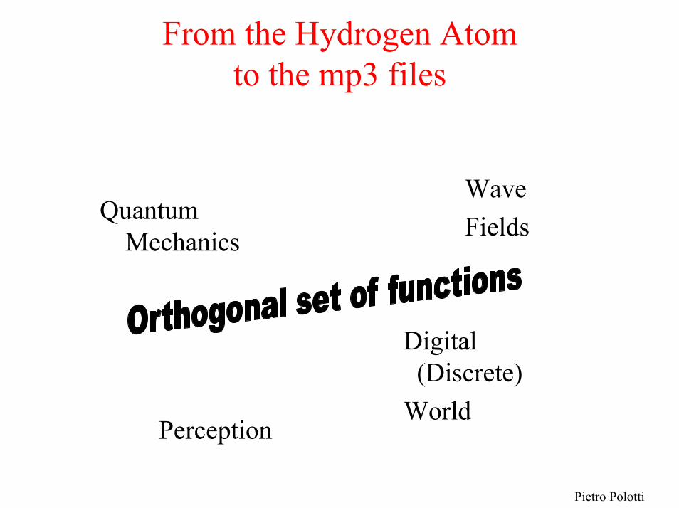
From the Hydrogen Atom to the mp3 files
WaveFields
Digital (Discrete)
World
Quantum Mechanics
Perception
Pietro Polotti
G. Essl and S. Zambon
• “PDE we use are quite related to Quantum Mechanics” (Essl)
• Bessel functions: Membrane oscillation.
• ANALOGY
OPTOMECHANICAL OPTICS MECHANICS
• Also... From Astronomy and Acoustics (Thompson) to Quantum Mechanics and DSP
• Legendre functions to decompose Sphere modes
• Laguerre Transform in order to obtain Frequency warping
Pietro Polotti
Adrien-Marie Legendre(1752-1833, Paris)
• Astronomer and mathematician
• He published about celestial mechanics with papers such as “Recherchessur la figure des planètes” (1784), which contains the Legendrepolynomials
• An elliptic function is an analytic function from C to C which is doubly periodic. That is, for two independent values of the complex number w, the functions f(z) and f(w + z) are the same.It can also be regarded as the inverse function to certain integrals (called elliptic integrals) of the form,
where R is a polynomial of degree 3 or 4.
∫ )(zRdz
Pietro Polotti
Edmond Nicolas Laguerre(1834, 1886 Bar-le-Duc, France)
•mathematician
– Laguerre polynomials which are solutions of the Laguerredifferential equations
– Laguerre Transform
Pietro Polotti
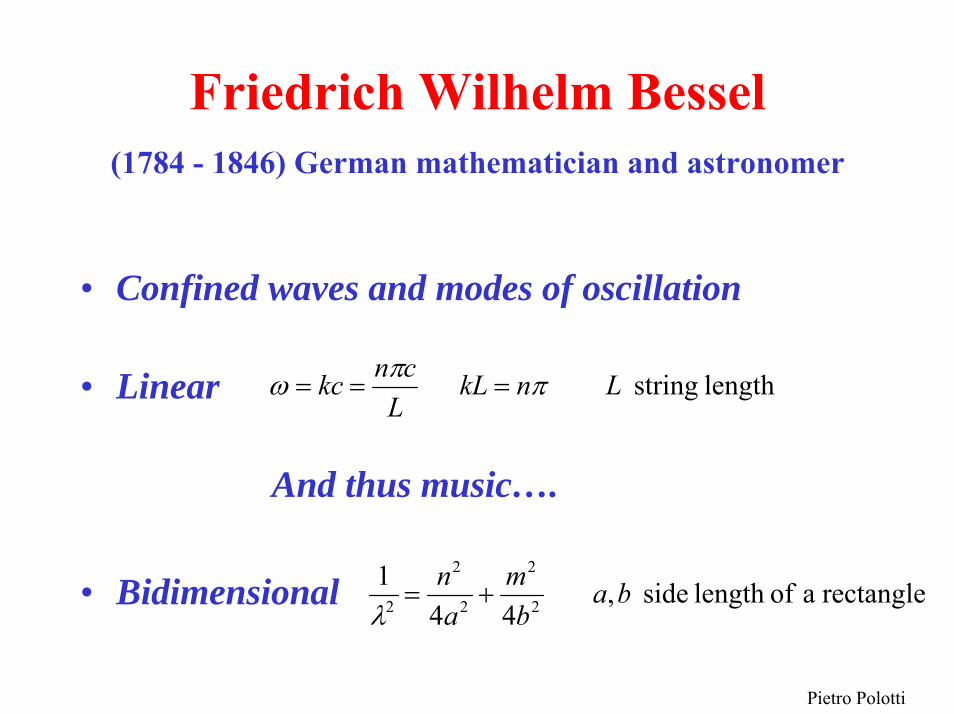
Friedrich Wilhelm Bessel(1784 - 1846) German mathematician and astronomer
• Confined waves and modes of oscillation
• Linear
And thus music….
• Bidimensional
length string LnkLL
cnkc ππω ===
rectangle a oflength side , 4
4
12
2
2
2
2 bab
man
+=λ
Pietro Polotti
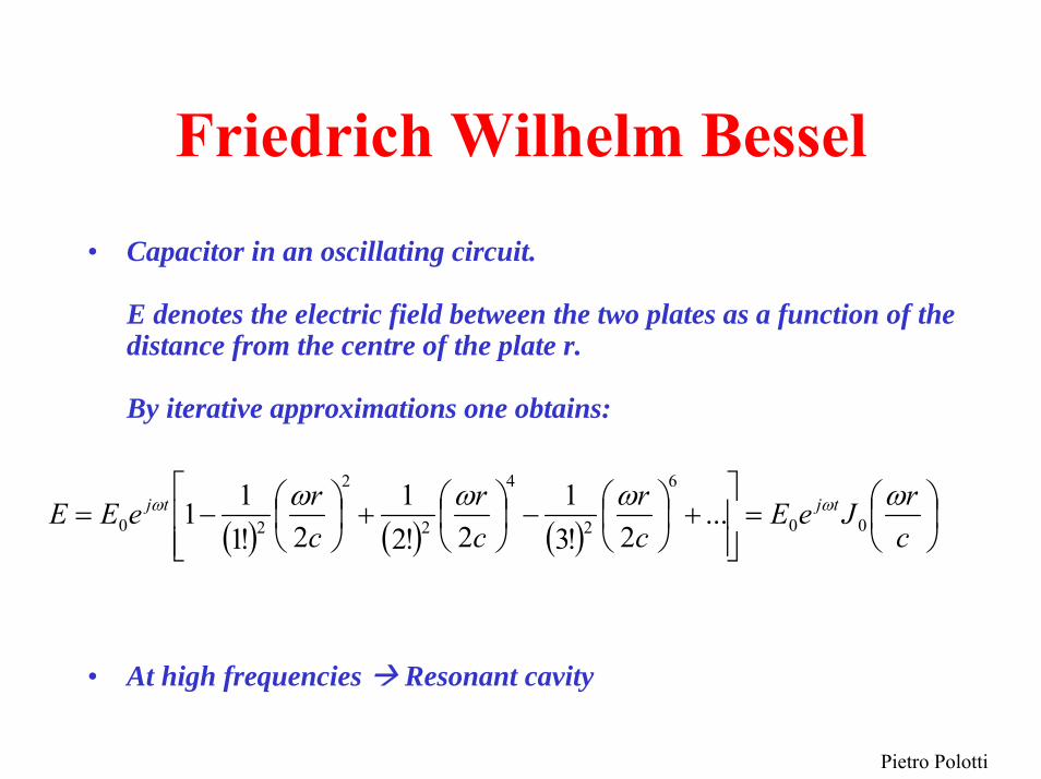
Friedrich Wilhelm Bessel• Capacitor in an oscillating circuit.
E denotes the electric field between the two plates as a function of the distance from the centre of the plate r.
By iterative approximations one obtains:
• At high frequencies Resonant cavity
( ) ( ) ( ) ⎟⎠⎞
⎜⎝⎛=
⎥⎥⎦
⎤
⎢⎢⎣
⎡+⎟
⎠⎞
⎜⎝⎛−⎟
⎠⎞
⎜⎝⎛+⎟
⎠⎞
⎜⎝⎛−=
crJeE
cr
cr
creEE tjtj ωωωω ωω
00
6
2
4
2
2
20 ...2!3
12!2
12!1
11
Pietro Polotti
J.J. Thompson(1856 - 1940)
• Also Thompson: from Astronomy and Acoustics toQuantum Mechanics
• In 1897 he discovered the first subatomic particle, a component of all atoms, the electron.

Pietro Polotti
Electrons play
• Acoustic waves• Stationary wave equation
• Stationary oscillationsmodes (Bessel functions in the case of circularsurfaces)
• Probability waves• Hamiltonian equation ot the
stationary states• Atomic orbitals
The electron “hits” (interacts with) the atomic “volume” (atomic force field) “generating” probability waves, representable as the combination of “modes” (eigenfunctions) of the Energy-Hamiltonian Equation.

Pietro Polotti
From the Hydrogen Atom to the mp3 files
An introduction to 2nd degree differential equations
Pietro Polotti
The crisis of the Classical Physics
• Radiations present particle-like behavior (Photoelectric effect)
• Particles present wave-like behavior (Diffraction)
• Nature is essentially discontinuous (Energy levels of the atomic orbital)
Pietro Polotti
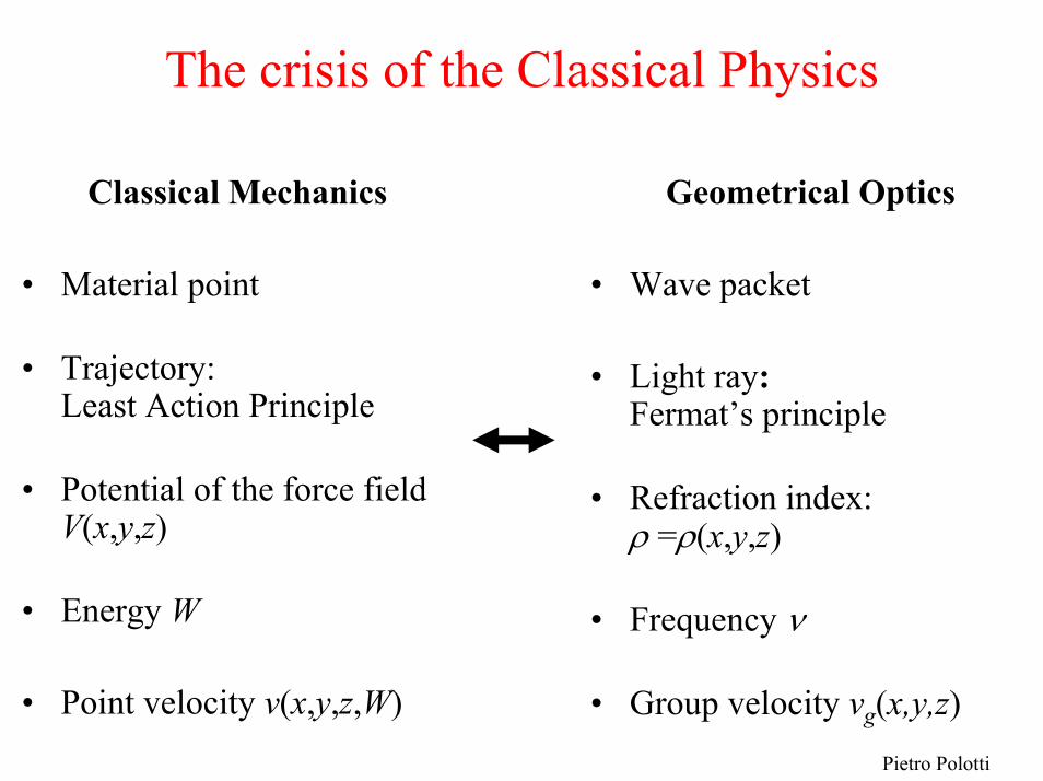
The crisis of the Classical Physics
Classical Mechanics
• Material point
• Trajectory: Least Action Principle
• Potential of the force field V(x,y,z)
• Energy W
• Point velocity v(x,y,z,W)
Geometrical Optics
• Wave packet
• Light ray: Fermat’s principle
• Refraction index: ρ =ρ(x,y,z)
• Frequency ν
• Group velocity vg(x,y,z)
Pietro Polotti
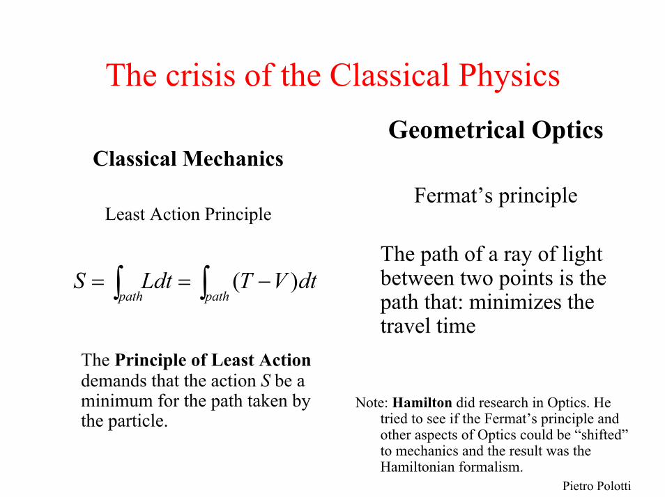
The crisis of the Classical PhysicsGeometrical Optics
Fermat’s principle
The path of a ray of light between two points is the path that: minimizes the travel time
Note: Hamilton did research in Optics. He tried to see if the Fermat’s principle and other aspects of Optics could be “shifted”to mechanics and the result was the Hamiltonian formalism.
Classical Mechanics
Least Action Principle
The Principle of Least Action demands that the action S be a minimum for the path taken by the particle.
∫∫ −==pathpath
dtVTLdtS )(
Pietro Polotti
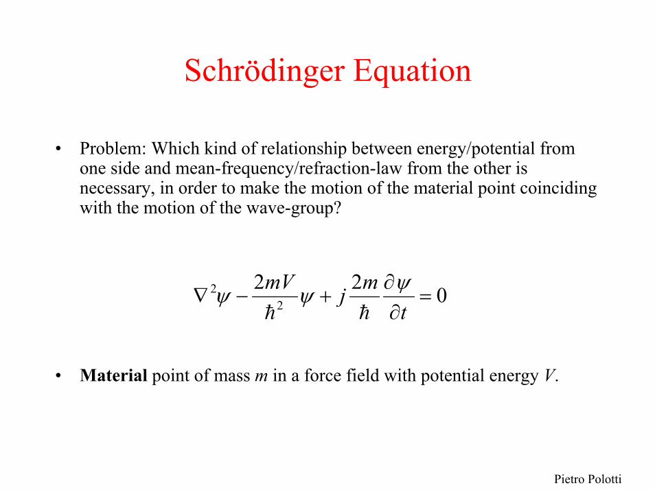
Schrödinger Equation
• Problem: Which kind of relationship between energy/potential from one side and mean-frequency/refraction-law from the other is necessary, in order to make the motion of the material point coinciding with the motion of the wave-group?
• Material point of mass m in a force field with potential energy V.
0222
2 =∂
∂+−∇
tmjmV ψψψ
Pietro Polotti
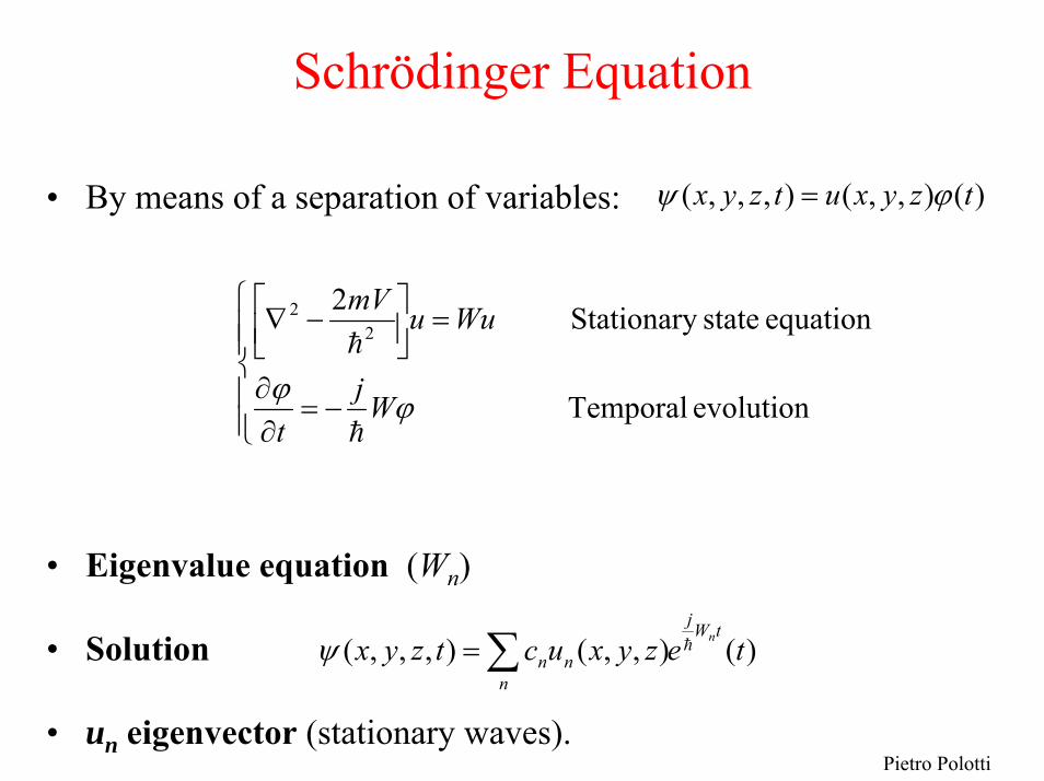
Schrödinger Equation
• By means of a separation of variables:
• Eigenvalue equation (Wn)
• Solution
• un eigenvector (stationary waves).
)(),,(),,,( tzyxutzyx ϕψ =
⎪⎪⎩
⎪⎪⎨
⎧
−=∂∂
=⎥⎦⎤
⎢⎣⎡ −∇
evolution Temporal
equation state Stationary 22
2
ϕϕ Wjt
WuumV
)(),,(),,,( tezyxuctzyxtWj
nnn
n∑=ψ

Pietro Polotti
Schrödinger Equation
• One can show that
• Thus from the condition
it follows:
• |cn|2 is interpreted as the probability of finding the value Wn when measuring the energy of the system.
( )
1 2
*
=
=
∑
∫
nn
mn
c
m-nδdxdydzuu
12 =∫ dxdydzψ

Pietro Polotti
Schrödinger Equation: The Operator Mechanics
• Let’s consider the Hamiltonian:
• Let’s “postulate” the correspondences
• We obtain an equality between two differential operators
• Multiplying by we obtain the Schroedinger Equation
EzyxVmp
EH i =+⇒= ∑ ),,(2
2
ii x
jp
tjE
∂∂
−→
∂∂
→
tjzyxV
m ∂∂
=+∇− ),,(2
22
2/2m−

Pietro Polotti
Building the Schroedinger Equation from the classical Hamiltonian
( ) ⎟⎟⎠
⎞⎜⎜⎝
⎛
∂∂
−=→= tq
iqHHtpqHHj
jQjjc ,, ,,
tiE
∂∂
→
( ) ( )t
tqitqH iiQ ∂
Ψ∂=Ψ
,,
• The Quantum Hamiltonian is an equation between operators that act on L2 functions of the qi ‘s and the time t.
• The same procedure can be applied for any classical physical observable
Pietro Polotti
General Structure of the Quantum Mechanics
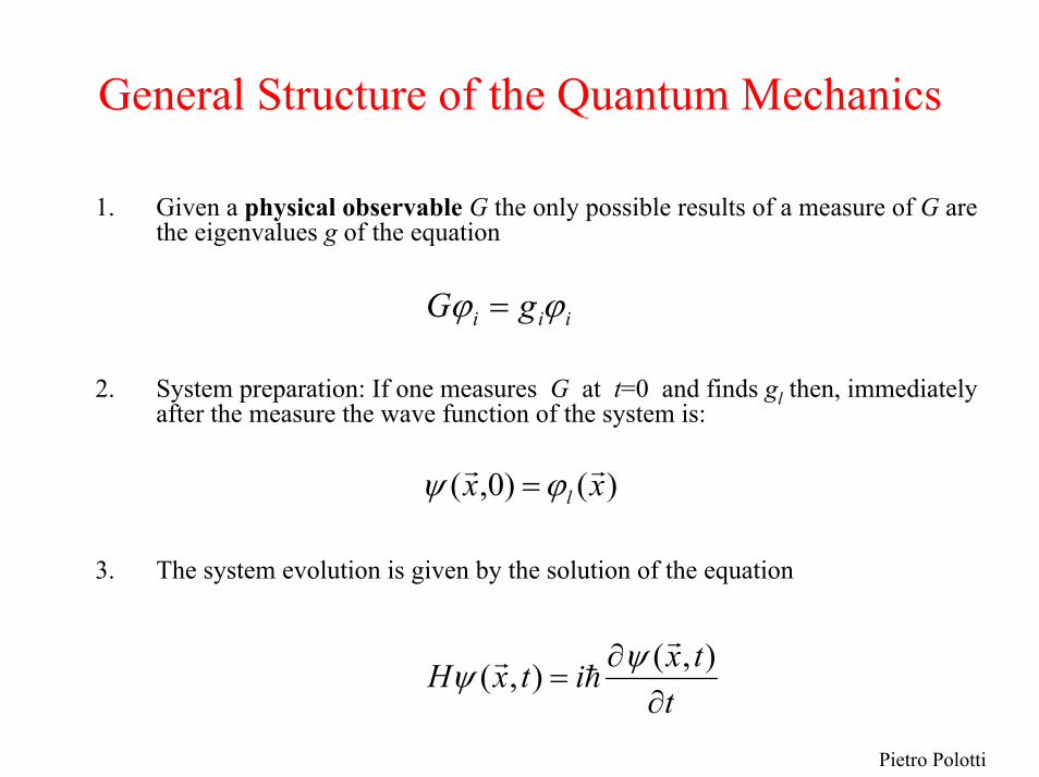
1. Given a physical observable G the only possible results of a measure of G are the eigenvalues g of the equation
2. System preparation: If one measures G at t=0 and finds gl then, immediately after the measure the wave function of the system is:
3. The system evolution is given by the solution of the equation
iii gG ϕϕ =
)()0,( xx lϕψ =
ttxitxH
∂∂
=),(),( ψψ
Pietro Polotti
General Structure of the Quantum Mechanics
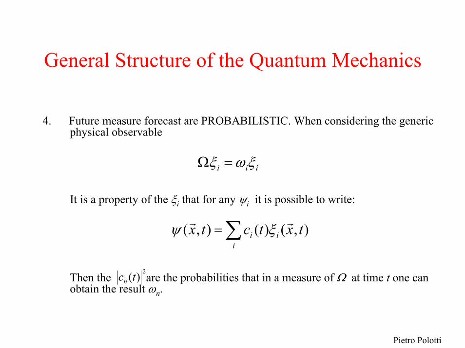
4. Future measure forecast are PROBABILISTIC. When considering the generic physical observable
It is a property of the ξi that for any ψi it is possible to write:
Then the are the probabilities that in a measure of Ω at time t one can obtain the result ωn.
iii ξωξ =Ω
2)(tcn
),()(),( txtctxi
ii∑= ξψ

Pietro Polotti
Uncertainty Principle (Werner Heisenberg, 1925)
• Classical Physics admit, at least in principle, the possibility of measuring simultaneously any couple of physical variable.
• As Achilles and the turtle, the more precise the measure instruments the more precise the measure, with non infinitesimal limitation
• BUT Reality is different
hpq ii ≥∆∆

Pietro Polotti
Linear Harmonic Oscillator• Steady state equation (classical Hamiltonian)
• Confluent Hypergeometric.
• Considering the asymptotic behavior of the solution, one finds that the solution include as a factor Hermit polynomial and from this follows that the energy must be:
( )
mx
xmxVu
xuxmEmdx
ud
πυ
υπ
υπ
21 frequency ticchracteris
2)( ionseigenfunctenergy
nt,displaceme 0 22
0
220
22022
2
=
=
=
==−+
⎟⎠⎞
⎜⎝⎛ +=
21
0 nhEn υ

Pietro Polotti
Towards the Hydrogen Atom
[ ] 0 )(2
22
=−−∇− urVEum
• Schroedinger equation for steady states
• Central force field
• Variable Separation: Radial and Angular components
)()( rVrV =
( ) ( ) ( ) ( )ϕθϕθ ΦΘ= rRru ,,
Pietro Polotti
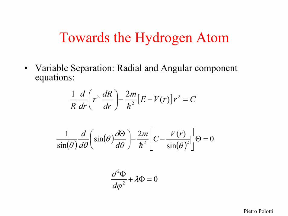
Towards the Hydrogen Atom
• Variable Separation: Radial and Angular component equations:
[ ] CrrVEmdrdRr
drd
R=−−⎟
⎠⎞
⎜⎝⎛ 2
22 )(21
( ) ( )( )
0 sin
)(2sinsin
122 =Θ⎥
⎦
⎤⎢⎣
⎡−−⎟
⎠⎞
⎜⎝⎛ Θ
θθθ
θθrVCm
dd
dd
02
2
=Φ+Φ λ
ϕdd

Pietro Polotti
Angular Momentum
( ) ( )( )
0 sin
)(2sinsin
122 =Θ⎥
⎦
⎤⎢⎣
⎡−−⎟
⎠⎞
⎜⎝⎛ Θ
θθθ
θθrVCm
dd
dd
It is an hypergeometric equation with fuchsian points: z = -1, 1, ∞
The solutions are:
With m and l parameters of the hypergeometric and Pl and Ql are Legendre functionsof the 1st and 2nd kind, respectively.
Note: By studying the asymptotic behavior one finds the eigenvalues: c= l(l+1)
( ) )()(, θθθ ml
mllm BQAP +=Θ

Legendre polynomials
( ) ( )11!2
1)()( 22/2 −−−= +
+
zdzdz
lzP ml
mlm
lmm
l
Angular Solution
Pietro Polotti

Pietro Polotti
Angular Solution
The global angular solutions are:
These are the Spherical Functions of order l and grade m and they satisfy the orthogonality condition:
.
( ) ( )( ) ( ) ( )
( )ϕ
θθθ
πϕθ jm
ml
mmmm
ml ed
PdmlmllY
coscossin
!!
412)(, 2/
, +−+
−= +
( ) ( )∫ ∫ =π π
δδϕθϕθθθϕ2
0',',
*','
0, ,, sin mmllmlml YYdd

Pietro Polotti
Radial Solution
The equation is now:
It can be reduced to an hypergeometric equation and by studying the behaviorat the infinity, the solution beomes:
Associated Laguerre functions
( ) ( )
charge nucleus
momentumangular theis 1 where 1 21 222
22
Z
llllrr
ZeEmdrdRr
drd
R++=⎥
⎦
⎤⎢⎣
⎡−−⎟
⎠⎞
⎜⎝⎛
( )( )
( ) )'( ' e ! 2! 12)'( 122
r'-3
3
0. rLr
lnnln
naZrR ll
lnl
ln+
+⎥⎥⎦
⎤
⎢⎢⎣
⎡
+−−
⎟⎟⎠
⎞⎜⎜⎝
⎛=
( ) )'(12 rL llln+
+
Pietro Polotti
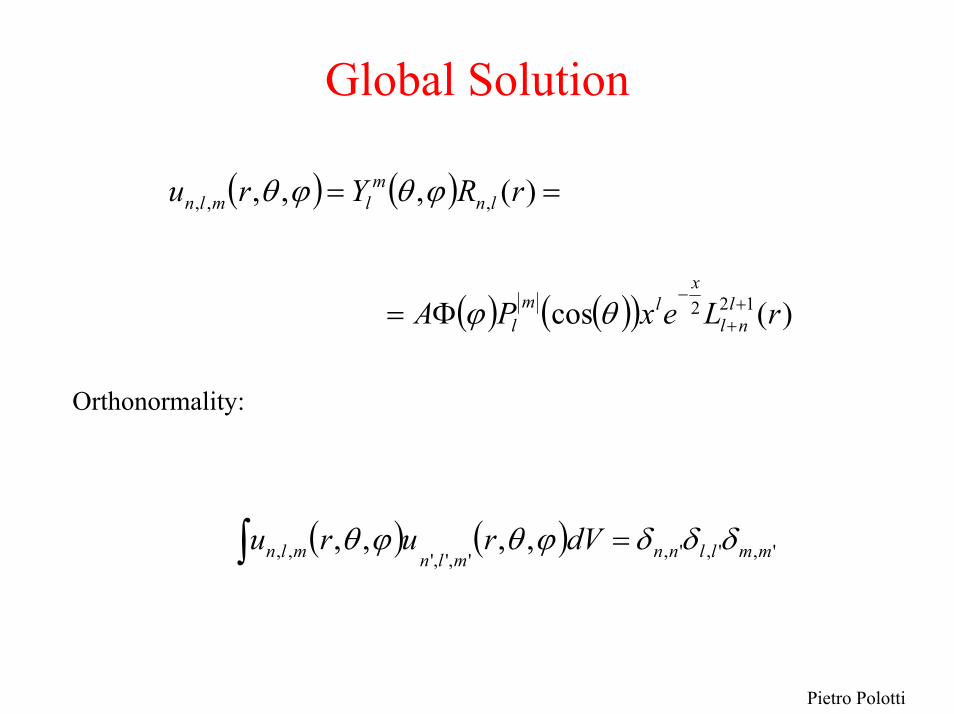
Global Solution
( ) ( )
( ) ( )( ) )(cos
)(,,,
122
,,,
rLexPA
rRYru
lnl
xlm
l
lnm
lmln
++
−Φ=
==
θϕ
ϕθϕθ
Orthonormality:
( ) ( ) ',',',',',',, ,,,, mmllnnmlnmln dVruru δδδϕθϕθ =∫

Pietro Polotti
Global Solution
The energy eigenvalues are:
They depend only on n. This happens only for the spherical symmetry case (1 electron)
l=0 orbitali sl=1 orbitali pl=2 orbitali dl=3 orbitali fl=4 orbitali g
2 2
42
2 neZmE n −=

Pietro Polotti
Bessel function for free particle
The radial component of the solution of the Schroedinger equation for a free particle
is,
where the Jl+1/2(ρ) are the cylindrical Bessel functions
( ) ( ) 0,,2,, 22 =+∇ ϕθψϕθψ rEmr
( )⎥⎥⎦
⎤
⎢⎢⎣
⎡⎟⎟⎠
⎞⎜⎜⎝
⎛+⎟⎟
⎠
⎞⎜⎜⎝
⎛=
−−+
mErBJmErAJCr
rRlll
221
21
21

Pietro Polotti
Bessel functions
• Bessel in the modes of a circular membrane
• Bessel in the FM
• Bessel in the Ambisonics
Pietro Polotti
From the Hydrogen Atom to the mp3 files
An Electrodynamic digression: Resonant cavities
Pietro Polotti
Hilbert space
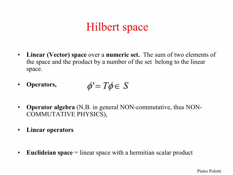
• Linear (Vector) space over a numeric set. The sum of two elements of the space and the product by a number of the set belong to the linear space.
• Operators,
• Operator algebra (N.B. in general NON-commutative, thus NON-COMMUTATIVE PHYSICS),
• Linear operators
• Euclideian space = linear space with a hermitian scalar product
ST ∈= φφ '

Pietro Polotti
Hilbert space
• Hermitian scalar product
S x S C a function with some properties:
a
b
c
• Norm
• Distance
( )ϕψ ,
( ) ( ) ( )2121 ,,, ϕψϕψϕϕψ baba +=+
( ) ( )*,, ψϕϕψ =
( ) ωϕϕϕ ==≥ iff "" 0,
( )[ ] 2/1,ψψψ =
ψφψφ −=,d
Pietro Polotti
Hilbert space
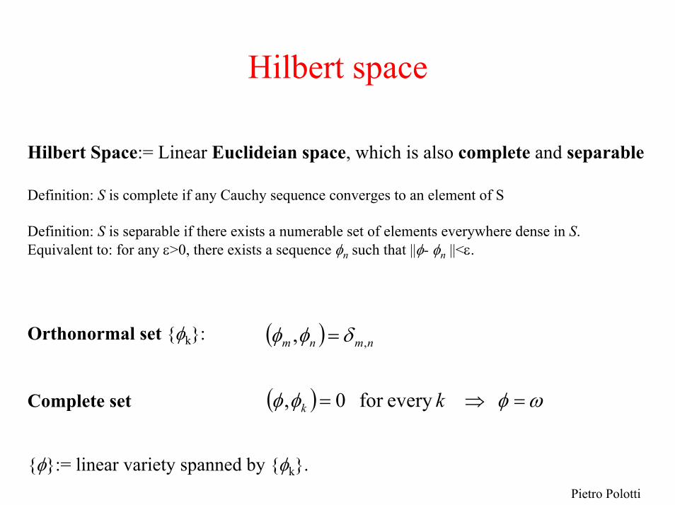
Hilbert Space:= Linear Euclideian space, which is also complete and separable
Definition: S is complete if any Cauchy sequence converges to an element of S
Definition: S is separable if there exists a numerable set of elements everywhere dense in S.Equivalent to: for any ε>0, there exists a sequence φn such that ||φ- φn ||<ε.
Orthonormal set φk:
Complete set
φ:= linear variety spanned by φk.
( ) , ,nmnm δφφ =
( ) ωφφφ =⇒= every for 0, kk
Pietro Polotti
Hilbert Spaces
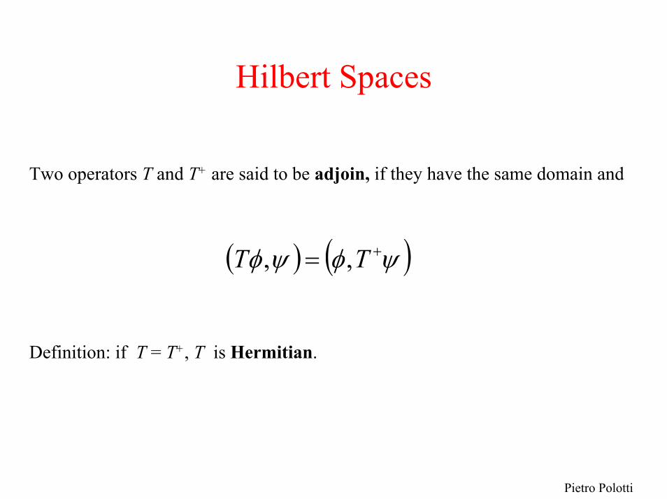
Two operators T and T+ are said to be adjoin, if they have the same domain and
Definition: if T = T+, T is Hermitian.
( ) ( )ψφψφ += TT ,,

Pietro Polotti
Hilbert Space
• Eigenvalue Equation
• The values hr for which the equation has solution form the Discrete Spectrum of H.
• Theorem : The Discrete Spectrum of a linear Hermitiantransformation is a set of points on the real axis empty, finite or infinite enumerable. Eigenvectors corresponding to different eigenvalues are orthogonal
(Furthermore the condition of Hermitianity implies real eigenvalues)
rrr hH φφ =

Pietro Polotti
Quantum Mechanics Hilbert Spaces
L(2)(∞) is the Euclideian space, whose elements are the complex functions of real variables, for which the following holds:
It is possible to make the space a vector (linear) space and an Euclideianspace, by defining:
It is possible to show that the space is also complete and separable, thus it is a Hilbert space.
( ) ∞<∫ ∫2
1,....,.... kqqf
),.....,(),.....,( 11 kk qqgqqfgf +=+
),.....,( 1 kqqff αα =
( ) ( ) ( ) kkk dqdqqqgqqfgf ....,....,,....,*...., 111∫ ∫=
Pietro Polotti
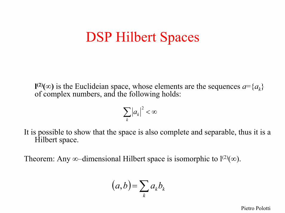
DSP Hilbert Spaces
l(2)(∞) is the Euclideian space, whose elements are the sequences a=akof complex numbers, and the following holds:
It is possible to show that the space is also complete and separable, thus it is a Hilbert space.
Theorem: Any ∞–dimensional Hilbert space is isomorphic to l(2)(∞).
∞<∑ 2
kka
( ) ∑=k
kkbaba,
Pietro Polotti
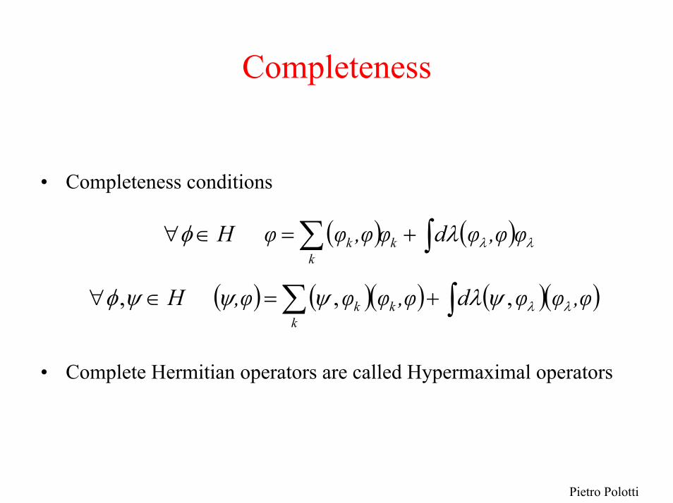
Completeness
• Completeness conditions
• Complete Hermitian operators are called Hypermaximal operators
( ) ( ) λλλφ φ,φφdφ,φφφH kk
k ∫∑ +=∈∀
( ) ( )( ) ( )( ),φφφd,φφφ,φHk
kk λλψλψψψφ ,, , ∫∑ +=∈∀

Pietro Polotti
Dirac Notation
βαψ ba +=
βαψ ** ba +=
Antilinear correspondence
Scalar product
φψ
Pietro Polotti
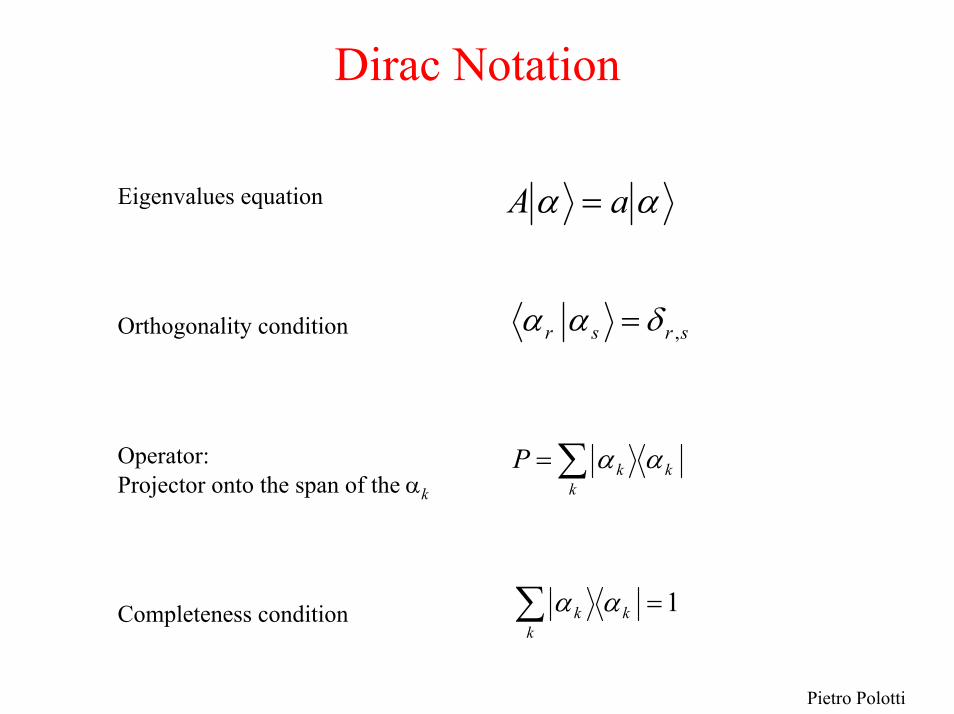
Dirac Notation
αα aA =Eigenvalues equation
Orthogonality condition
Operator:Projector onto the span of the αk
Completeness condition
srsr ,δαα =
∑=k
kkP αα
1=∑k
kk αα
Pietro Polotti
Quantum Mechanics General Postulates
• Physical variable Hypermaximal operator.
• The only possible values of a measure are the eigenvalues.
• Immediately after a measure the system falls into the state corresponding to an eigenvector.
• The system evolves according to the Schroedingerequation.
• Future measures are predictable in terms of the probabilities |ck|2 , where the ck are the eigenvalues of a certain physical variable.

Pietro Polotti
Quantum Mechanics General Postulates
• We say that the measure projects the system onto one of the possible stationary state of the physical variable.
• Quantum Mechanics is the Physics of the Projection Operators, i.e. of the orthogonal expansion!
Pietro Polotti
General Structure of the Quantum Mechanicsaddendum
• We say that the measure projects the system onto one of the possible stationary state of the physical variable.
• Quantum Mechanics is the Physics of the Projection Operators, i.e. of the orthogonal expansion!
Pietro Polotti
Electrons play
Acoustics / Electrodynamics / Quantum Mechanics
Applets
http://www.falstad.com/mathphysics.html
Pietro Polotti
The Point
• DUE TO QUANTUM MECHANICS AND THE CENTRALITY OF THE STEADY STATE EQUATION, THE SOLUTION OF EIGENVALUE EQUATIONSAND THE EXPANSION OF THEIR SOLUTIONS ON THE EIGENVECTOR BASIS BECOME A CENTRAL PROBLEM.
• THIS FORMALISM FIND EQUIVALENCIES WITH AND CAN BE TRASPOSED TO MANY OTHER FIELDS OF PHYSICS AND OTHER SCIENTIFIC CONTEXTS.
Pietro Polotti
The Point: QM “reminiscences” in DSP
Atomic Orbitals ↔ Subband-Coding
Position/Momentum Uncertainty
Time/Frequency Uncertainty
Pietro Polotti
l2 : the “DSP Hilbert Space”
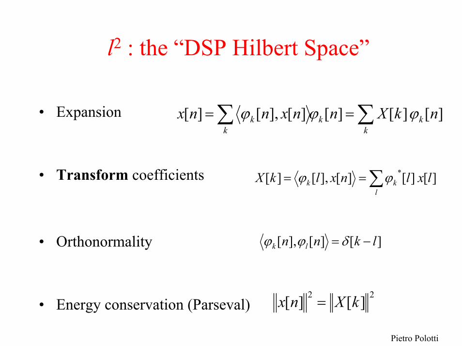
• Expansion
• Transform coefficients
• Orthonormality
• Energy conservation (Parseval)
][ ][][][],[][ nkXnnxnnx kk
kk
k ϕϕϕ ∑∑ ==
][ ][][],[][ * lxlnxlkXl
kk ∑== ϕϕ
][][],[ lknn lk −= δϕϕ
22 ][][ kXnx =
Pietro Polotti
l2 : the “DSP Hilbert Space”
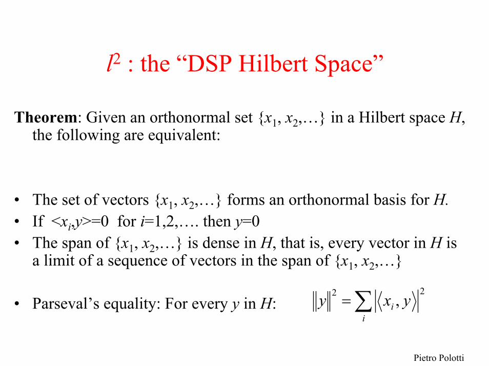
Theorem: Given an orthonormal set x1, x2,… in a Hilbert space H, the following are equivalent:
• The set of vectors x1, x2,… forms an orthonormal basis for H.• If <xi,y>=0 for i=1,2,…. then y=0• The span of x1, x2,… is dense in H, that is, every vector in H is
a limit of a sequence of vectors in the span of x1, x2,…
• Parseval’s equality: For every y in H:22 ,∑=
ii yxy

Pietro Polotti
l2 : the “DSP Hilbert Space”
Given a Hilbert space H and a closed subspace V0, such that:
H= V0⊕W0,
where W0 is said to be the orthogonal complement of V0 in H, then,if u ∈H
u=v+w ,where v ∈ V0 and w ∈ W0
Definition: An operator P is called a projection operator onto V0 if
P(u)= P(v+w)=v
An operator is a projection operator iff it isIdempotent: P2=PSelf adjoint: P*=P

Pietro Polotti
l2 : the “DSP Hilbert Space”
• Space decomposition V0⊥W0 ⇒ V0⊕W0=V-1
• Design of orthogonal FIR filter banks

Pietro Polotti
Sampling Theorem
The set sinc(t-l), l ∈ Z forms an othonormal basis for the set of functions f(t) bandlimited to (-π,π), where
• Even the most simple coding technique (PCM) is done by means of an expansion onto an othonormal set of functions
πtπtt )sin()sinc( =
Pietro Polotti
Sampling Representations
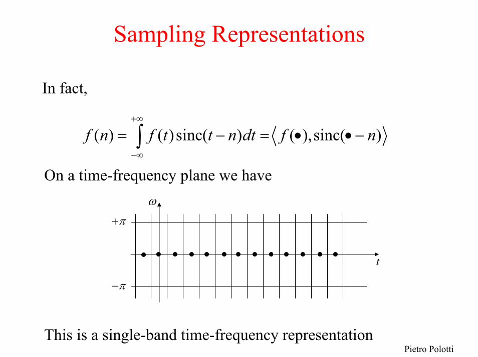
In fact,
( ) ( )sinc( ) ( ),sinc( )f n f t t n dt f n+∞
−∞
= − = • • −∫On a time-frequency plane we have
ω
+π
t
−π
This is a single-band time-frequency representation
Pietro Polotti
Multirate DSPOrthogonal Filter Banks
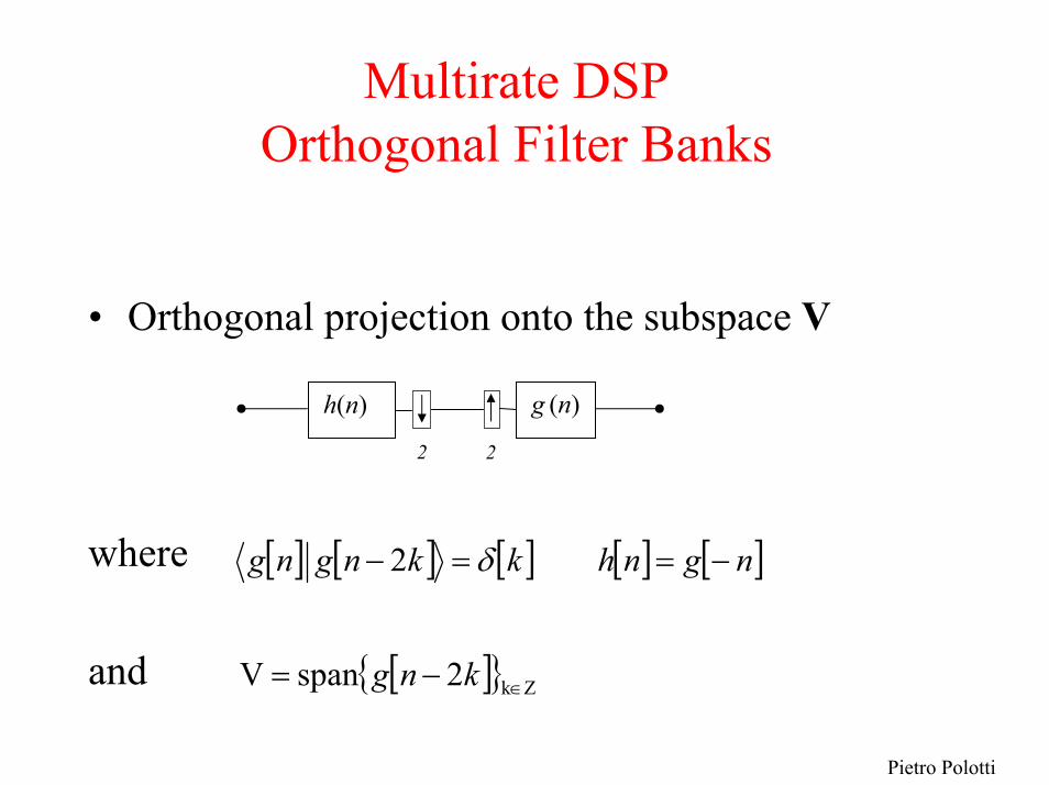
• Orthogonal projection onto the subspace V
where
and
g (n)h(n)
2 2
[ ] [ ] [ ] [ ] [ ]ngnhkkngng −==− 2 δ
[ ] 2spanV Zk∈−= kng
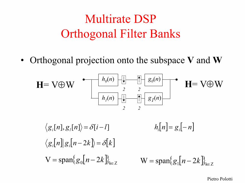
• Orthogonal projection onto the subspace V and W
[ ] [ ] [ ]kkngng ii δ=− 2
[ ] 2spanV Zk0 ∈−= kng
Multirate DSPOrthogonal Filter Banks
g0(n)h0(n)2 2
g1(n)h1(n)2 2
[ ] [ ]ngnhlingng iili −=−= ][][],[ δ
H= V⊕W
[ ] 2spanW Zk1 ∈−= kng
H= V⊕W
Pietro Polotti
Pietro Polotti
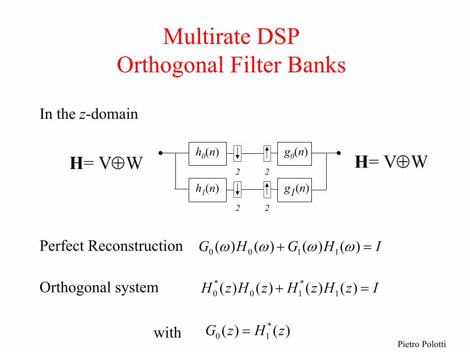
Multirate DSPOrthogonal Filter Banks
In the z-domain
Perfect Reconstruction
Orthogonal system
with
g0(n)h0(n)2 2
g1(n)h1(n)2 2
H= V⊕WH= V⊕W
IHGHG =+ )()()()( 1100 ωωωω
)()()()( 1*10
*0 IzHzHzHzH =+
)()( *10 zHzG =
Pietro Polotti
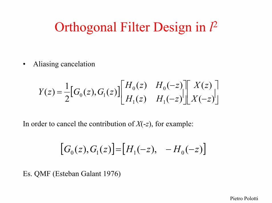
Orthogonal Filter Design in l2
• Aliasing cancelation
In order to cancel the contribution of X(-z), for example:
Es. QMF (Esteban Galant 1976)
[ ] ⎥⎦
⎤⎢⎣
⎡−⎥
⎦
⎤⎢⎣
⎡−−
=)(
)()()()()(
)(),(21)(
11
0010 zX
zXzHzHzHzH
zGzGzY
[ ] [ ])(),( )(),( 0110 zHzHzGzG −−−=
Pietro Polotti
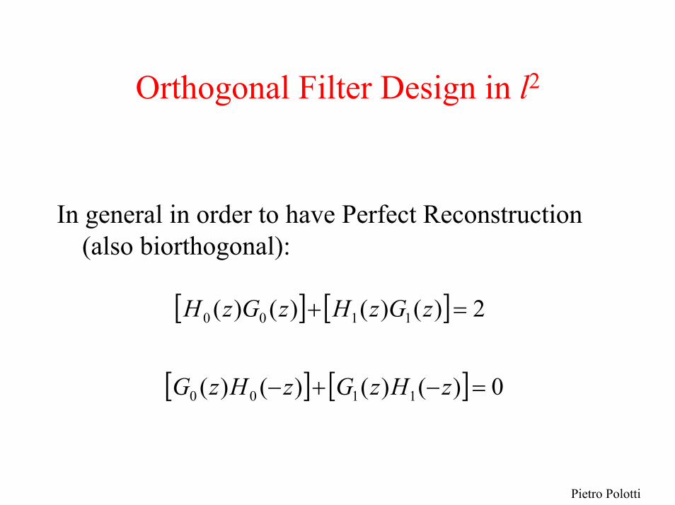
Orthogonal Filter Design in l2
In general in order to have Perfect Reconstruction (also biorthogonal):
[ ] [ ] 2)()()()( 1100 =+ zGzHzGzH
[ ] [ ] 0)()()()( 1100 =−+− zHzGzHzG
Pietro Polotti
Orthogonal Filter Design in l2
• Haar the simplest wavelet:
– orthogonal
– linear phase
– FIR
Pietro Polotti
Haar
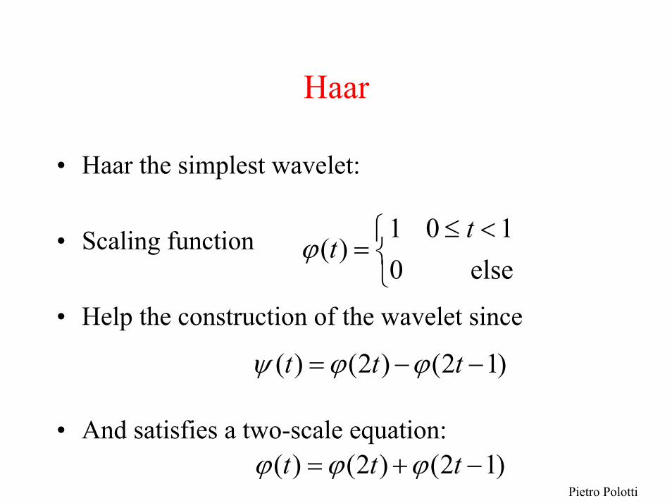
• Haar the simplest wavelet:
• Scaling function
• Help the construction of the wavelet since
• And satisfies a two-scale equation:
⎩⎨⎧ <≤
=else 0
10 1)(
ttϕ
)12()2()( −−= ttt ϕϕψ
)12()2()( −+= ttt ϕϕϕ

Pietro Polotti
Discrete Haar
[ ]⎪⎪
⎩
⎪⎪
⎨
⎧
+=−
=
=+
otherwise 0
12for 2
1
2for 2
1
12 kn
kn
nkϕ[ ]⎪⎩
⎪⎨⎧ +==
otherwise 0
12,2for 2
12
kknnkϕ
φ0(n)φ0(-n)2 2
φ1(n)φ1(-n)2 2

Pietro Polotti
Time vs. Frequency RepresentationsFor the frequency representation the orthogonal set elements are complex sinusoids with
2 ( )j t FTe πδ ωΩ ⎯⎯→ − Ω
On a time-frequency plane we have:
2πδ(ω-Ω)infinitely good in frequency,infinitely bad in time
t
ω
δ(t-τ)infinitely good in time,infinitely bad in frequency
Pietro Polotti
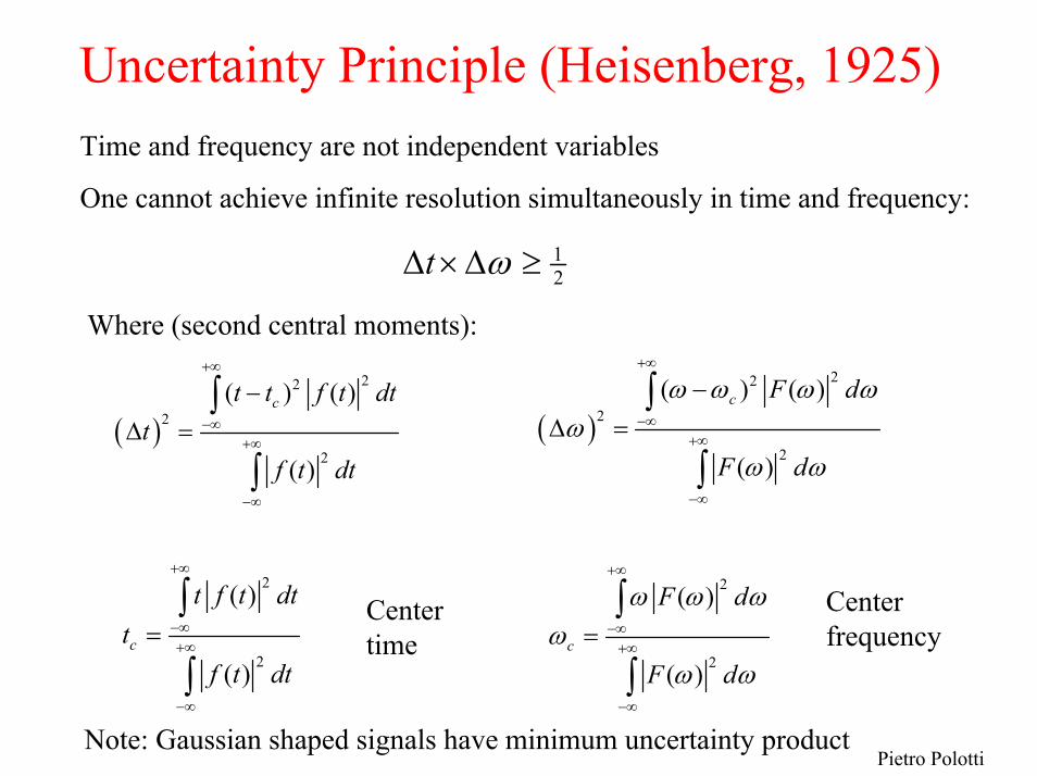
Uncertainty Principle (Heisenberg, 1925)Time and frequency are not independent variables
One cannot achieve infinite resolution simultaneously in time and frequency:
12t ω∆ × ∆ ≥
Where (second central moments):
( )
22
2
2
( ) ( )
( )
c F d
F d
ω ω ω ωω
ω ω
+∞
−∞+∞
−∞
−∆ =
∫
∫( )
22
2
2
( ) ( )
( )
ct t f t dtt
f t dt
+∞
−∞+∞
−∞
−∆ =
∫
∫
2
2
( )
( )c
t f t dtt
f t dt
+∞
−∞+∞
−∞
=∫
∫
2
2
( )
( )c
F d
F d
ω ω ωω
ω ω
+∞
−∞+∞
−∞
=∫
∫Note: Gaussian shaped signals have minimum uncertainty product
Center frequency
Center time
Pietro Polotti
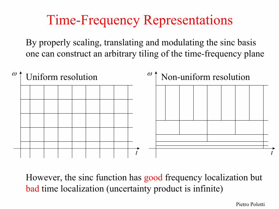
Time-Frequency RepresentationsBy properly scaling, translating and modulating the sinc basis one can construct an arbitrary tiling of the time-frequency plane
ω ωUniform resolution Non-uniform resolution
t t
However, the sinc function has good frequency localization but bad time localization (uncertainty product is infinite)

Pietro Polotti
Short-Time Fourier TransformUniform (Gabor’s) expansion is realized by means of the STFT
2
21
0
For discrete-time signals
( , ) ( ) ( ) (analysis)
1 ( ) ( , ) ( ) (synthesis)
with ( ) finite-length
j kmN
k
N j nmN
m r
F n m f k w k nM e
f n e F r m w n rMN
w n
π
π
+∞ −
=−∞
− +∞
= =−∞
= −
= −
∑
∑ ∑
window and ( ) satisfying
( ) ( ) 1 r
N w n
w n rM w n rM n+∞
=−∞
− − = ∀ ∈∑ Z
This is the overlap-add method for the product of the windows ( ) ( )w n w n
Pietro Polotti
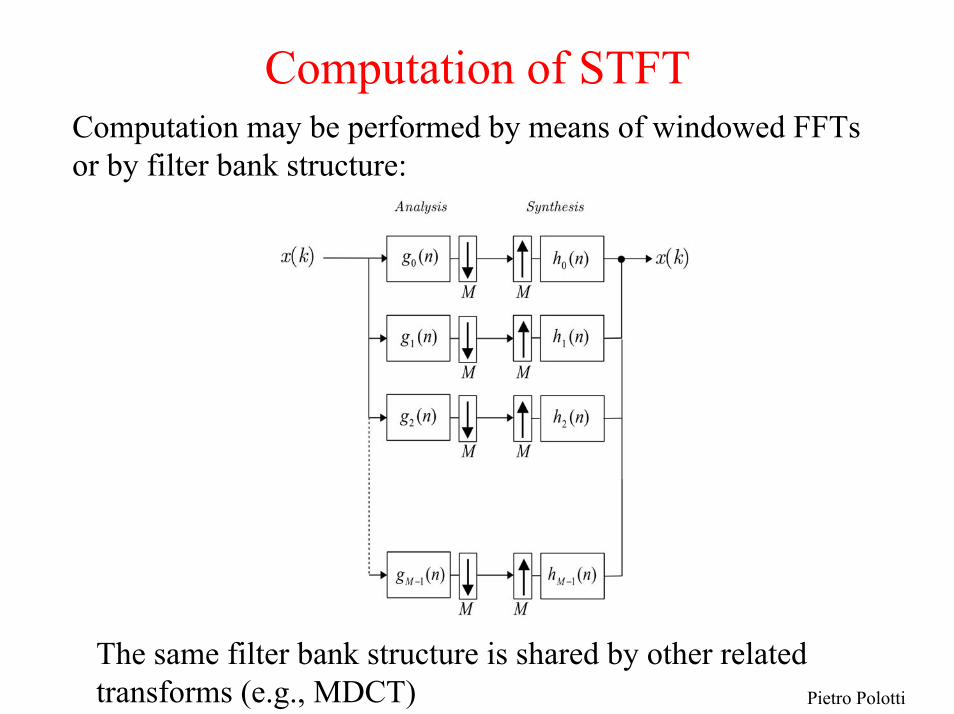
Computation of STFTComputation may be performed by means of windowed FFTsor by filter bank structure:
The same filter bank structure is shared by other related transforms (e.g., MDCT)
Pietro Polotti
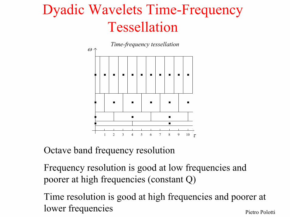
Dyadic Wavelets Time-Frequency Tessellation
ωTime-frequency tessellation
1 2 3 4 5 6 7 8 9 10 τ
Octave band frequency resolution
Frequency resolution is good at low frequencies and poorer at high frequencies (constant Q)
Time resolution is good at high frequencies and poorer at lower frequencies
Pietro Polotti
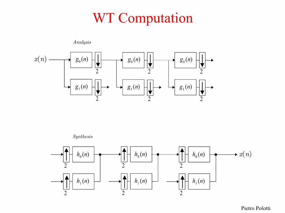
WT Computation
Pietro Polotti
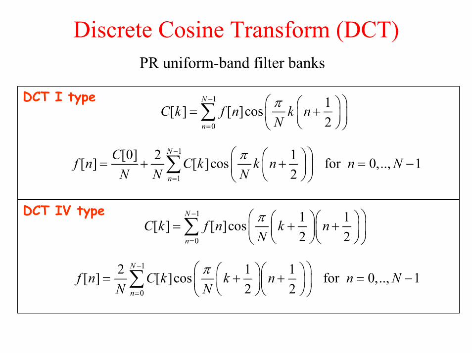
Discrete Cosine Transform (DCT) PR uniform-band filter banks
DCT I type
1
1
[0] 2 1[ ] [ ]cos for 0,.., 12
π−
=
⎛ ⎞⎛ ⎞= + + = −⎜ ⎟⎜ ⎟⎝ ⎠⎝ ⎠
∑N
n
Cf n C k k n n NN N N
1
0
1[ ] [ ]cos2
π−
=
⎛ ⎞⎛ ⎞= +⎜ ⎟⎜ ⎟⎝ ⎠⎝ ⎠
∑N
n
C k f n k nN
DCT IV type
1
0
2 1 1[ ] [ ]cos for 0,.., 12 2
π−
=
⎛ ⎞⎛ ⎞⎛ ⎞= + + = −⎜ ⎟⎜ ⎟⎜ ⎟⎝ ⎠⎝ ⎠⎝ ⎠
∑N
n
f n C k k n n NN N
1
0
1 1[ ] [ ]cos2 2
π−
=
⎛ ⎞⎛ ⎞⎛ ⎞= + +⎜ ⎟⎜ ⎟⎜ ⎟⎝ ⎠⎝ ⎠⎝ ⎠
∑N
n
C k f n k nN

Pietro Polotti
Modified Discrete Cosine Transform (MDCT) By means of DCT-I or DCT-IV one can build PR and
orthogonal uniform-band cosine modulated filter banks
MDCT from DCT IV type
2 1 1[ ] [ ] cos length 22 2
π⎛ + ⎞⎛ ⎞⎛ ⎞= + +⎜ ⎟⎜ ⎟⎜ ⎟⎝ ⎠⎝ ⎠⎝ ⎠
kMh n W n k n M
M M
1[ ] sin2 2π ⎛ ⎞= +⎜ ⎟
⎝ ⎠W n n
M
2 2[ ] [ ] 1[2 1 ] [ ]
⎧ + + =⎨
− − =⎩
W n W n MW M n W n
examplewhere
(2 1) center frequencies of the filters2
πω +=k
kM

Pietro Polotti
MR DSP MDCT completeness and orthogonality
conditions
• Completeness
• Orthogonality
( )( ) ( )( ) ',
1
01'2
412 cos12
412 cos )'( )( 1
llr
P
qPrPl
PqPrPl
PqrPlWrPlW
Pδππ =⎟
⎠⎞
⎜⎝⎛ +−−
+⎟⎠⎞
⎜⎝⎛ +−−
+−−∑ ∑
∞
−∞=
−
=
( )( ) ( )( ) ',',1'24
1'2 cos124
12 cos)'()(1rrqq
lPPrl
PqPrPl
PqPrlWrPlW
Pδδππ =⎟
⎠⎞
⎜⎝⎛ +−−
+⎟⎠⎞
⎜⎝⎛ +−−
+−−∑
∞
−∞=

Pietro Polotti
Compression Methods
Lossy compression:
1) MDCT subband decomposition
2) STFT in order to estimate the psychoacoustic model parameters
3) Dynamic bit allocation according to the psychoacustic param. (signal-to-mask ratio SMR)
4) Quantization and entropy coding of subbandsignals
5) Multiplex and frame packing

Pietro Polotti
MPEG1-layer 3 (*.mp3)
• MPEG (Motion Picture Experts Group): gruppo di scienziati che studiano codifiche standard per la compressione video e audio
• MPEG1 (layer 1, 2, 3)
• L’orecchio non è in grado di percepire frequenze “deboli” adiacenti a frequenze “forti”, che mascherano le prime.
• Le informazioni inerenti le frequenze più deboli vengono eliminate dall’MPEG durante la fase di compressione.

Pietro Polotti
1) Absolute Threshold
Non uniform hearing capabilities along the frequency range
( ) ( ) ( ) ( ) SPL) (dB 100010561000643 433310006080 2
fe.-f.fAbsTh -.-f.-. ⋅+⋅⋅= −

Pietro Polotti
2) Basilar Membrane and Critical Bands
• The cochlear “continuos passband filters”are of non-uniform bandwidth
• Discrete version: Critical Bands → Bark subdivision of FD
(Hz) ])1000/(4.11[7525)( 69.02ffBWc ++=
( ) ( ) (Bark) 7500
arctan5.300076.0arctan132
⎥⎥⎥
⎤
⎢⎢⎢
⎡
⎥⎥⎦
⎤
⎢⎢⎣
⎡⎟⎠⎞
⎜⎝⎛⋅+⋅⋅=
fffB

Pietro Polotti
Critical Band Subdivision
Representing the ear as a passband filter bank with non-uniform bandwidth

Pietro Polotti
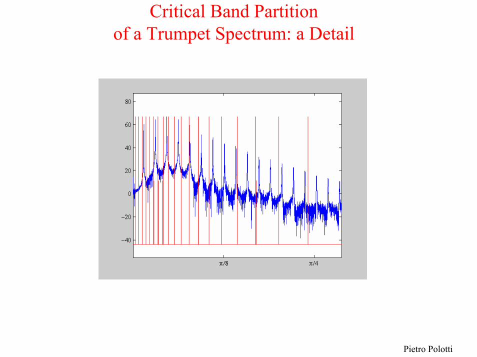
Critical Band Partition of a Trumpet Spectrum
Non uniform distribution of the partials in the Bark subdivision
Pietro Polotti
Critical Band Partition of a Trumpet Spectrum: a Detail
Pietro Polotti
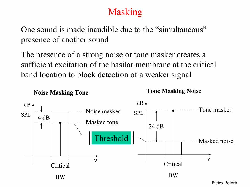
Masking
One sound is made inaudible due to the “simultaneous”presence of another sound
The presence of a strong noise or tone masker creates a sufficient excitation of the basilar membrane at the critical band location to block detection of a weaker signal
Tone Masking Noise
dB
SPL
Noise Masking Tone
νCritical
BW
Noise masker
Masked tone4 dB
dB
SPL
Noise Masking Tone
νCritical
BW
Noise masker
Masked tone4 dB
Threshold24 dB
dB
SPL
νCritical
BW
Tone masker
Masked noise

Pietro Polotti
3) Tone–Masking-Noise (TMN)
Signal-to-Mask Ratio (SMR) = 24 dB for TMN case
SMR
Asymmetric Spread of Masking Threshold
Absolute Threshold
Pietro Polotti
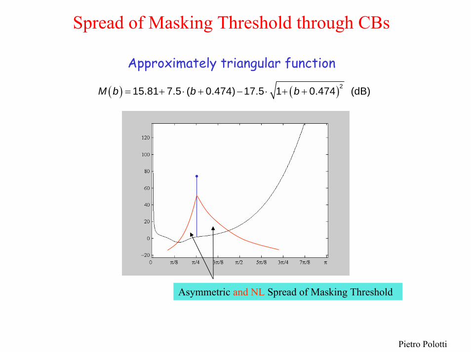
Spread of Masking Threshold through CBs
Approximately triangular function
( ) ( )215.81 7.5 ( 0.474) 17.5 1 0.474 (dB)M b b b= + ⋅ + − ⋅ + +
Asymmetric and NL Spread of Masking Threshold

Pietro Polotti
Real case: 1 TMN

Pietro Polotti
Real case: 2 TMN
Pietro Polotti
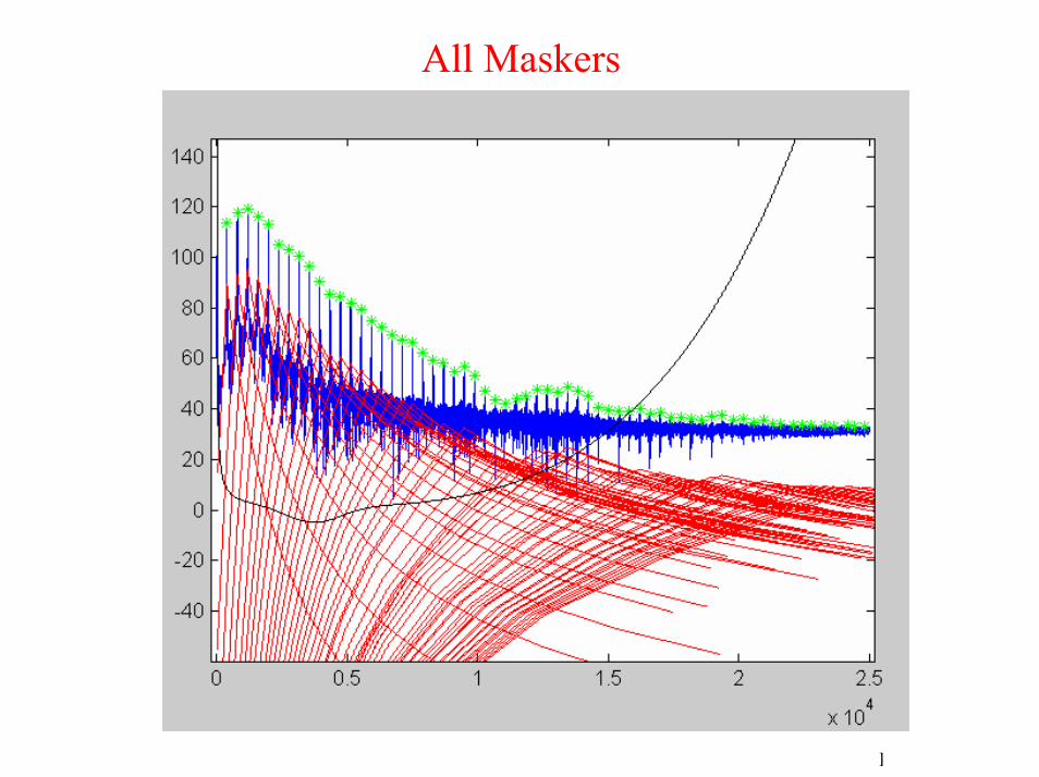
All Maskers
Pietro Polotti
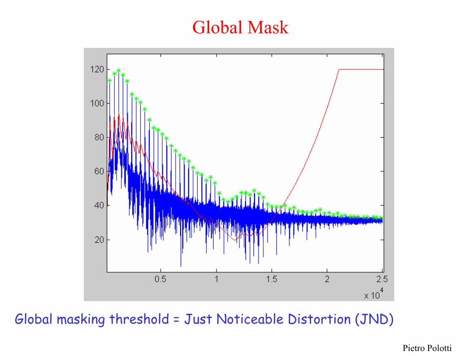
Global Mask
Global masking threshold = Just Noticeable Distortion (JND)

Pietro Polotti
Short-Time Thresholds Evaluation
Pietro Polotti
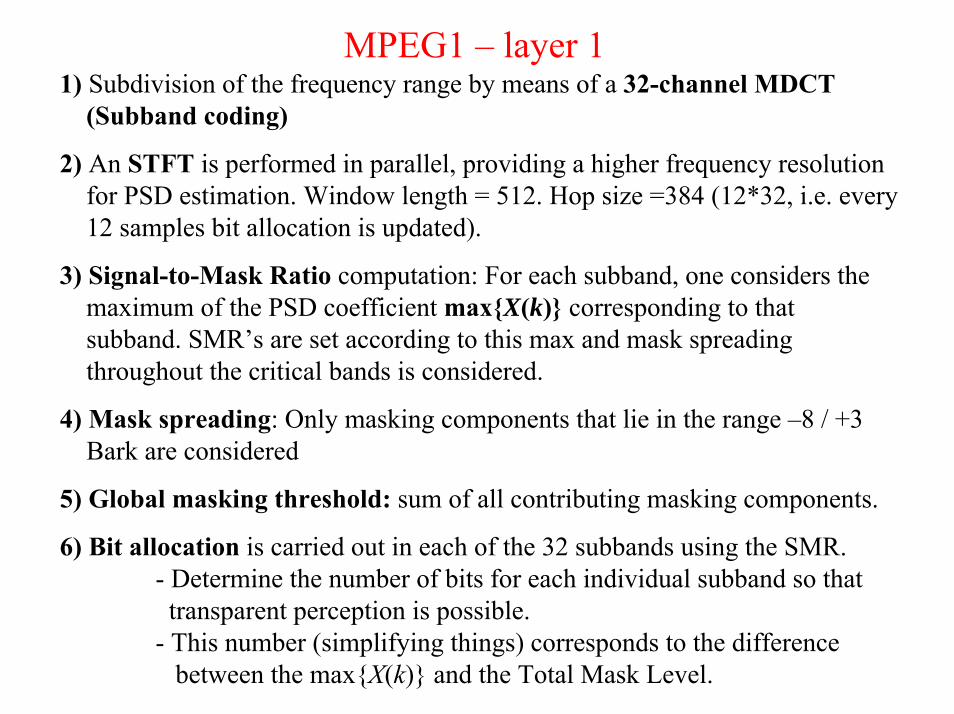
MPEG1 – layer 11) Subdivision of the frequency range by means of a 32-channel MDCT
(Subband coding)
2) An STFT is performed in parallel, providing a higher frequency resolution for PSD estimation. Window length = 512. Hop size =384 (12*32, i.e. every 12 samples bit allocation is updated).
3) Signal-to-Mask Ratio computation: For each subband, one considers the maximum of the PSD coefficient maxX(k) corresponding to that subband. SMR’s are set according to this max and mask spreading throughout the critical bands is considered.
4) Mask spreading: Only masking components that lie in the range –8 / +3 Bark are considered
5) Global masking threshold: sum of all contributing masking components.
6) Bit allocation is carried out in each of the 32 subbands using the SMR.- Determine the number of bits for each individual subband so that transparent perception is possible.
- This number (simplifying things) corresponds to the difference between the maxX(k) and the Total Mask Level.

Pietro Polotti
MPEG1 – layer 1
Compression algorithm Scheme