from the colour glass condensate to filamentation
TRANSCRIPT
Eur. Phys. J. C (2019) 79:286https://doi.org/10.1140/epjc/s10052-019-6790-8
Regular Article - Theoretical Physics
From the colour glass condensate to filamentation:systematics of classical Yang–Mills theory
Owe Philipsen1,2,a, Björn Wagenbach1,2,b, Savvas Zafeiropoulos3,c
1 Institut für Theoretische Physik, Goethe-Universität Frankfurt am Main, Max-von-Laue-Str. 1, 60438 Frankfurt, Germany2 John von Neumann Institute for Computing (NIC), GSI, Planckstr. 1, 64291 Darmstadt, Germany3 Institut für Theoretische Physik, Universität Heidelberg, Philosophenweg 12, 69120 Heidelberg, Germany
Received: 16 October 2018 / Accepted: 14 March 2019 / Published online: 28 March 2019© The Author(s) 2019
Abstract The non-equilibrium early time evolution of anultra-relativistic heavy ion collision is often described byclassical lattice Yang–Mills theory, starting from the colourglass condensate (CGC) effective theory with an anisotropicenergy momentum tensor as initial condition. In this workwe investigate the systematics associated with such studiesand their dependence on various model parameters (IR, UVcutoffs and the amplitude of quantum fluctuations) whichare not yet fixed by experiment. We perform calculations forSU(2) and SU(3), both in a static box and in an expandinggeometry. Generally, the dependence on model parametersis found to be much larger than that on technical parameterslike the number of colours, boundary conditions or the lat-tice spacing. In a static box, all setups lead to isotropisationthrough chromo-Weibel instabilities, which is illustrated bythe accompanying filamentation of the energy density. How-ever, the associated time scale depends strongly on the modelparameters and in all cases is longer than the phenomenolog-ically expected one. In the expanding system, no isotropisa-tion is observed for any parameter choice. We show howinvestigations at fixed initial energy density can be used tobetter constrain some of the model parameters.
1 Introduction
The medium created by ultra-relativistic heavy-ion collisionsis characterised by strong collective behaviour. It is generallyaccepted that a quark-gluon plasma (QGP) is formed and theeffective theory describing the multiparticle correlations ofthis nearly-perfect fluid is relativistic viscous hydrodynam-ics. For a long time it was believed that the application of
a e-mail: [email protected] e-mail: [email protected] e-mail: [email protected]
hydrodynamic models requires the thermalisation time fromthe initial non-equilibrium stage of the collision to the QGPto be very short [1,2] compared to the lifetime of the QGP.More recently it was argued that hydrodynamics also appliesto a not-yet equilibrated system [3].
From a theoretical point of view, a heavy-ion collisionhas different stages. As an initial condition, one assumes thecolour glass condensate (CGC), i.e. an effective field theorydescription of boosted, saturated gluons [4]. The resultingstrong gauge field dynamics constitutes the first stage of theevolution. A following later stage is then governed by hydro-dynamic equations until the medium becomes too dilute forthis long wavelength description. The precise duration of theearly stage is not yet known for realistic values of the cou-pling. Models of the hydrodynamical stage constrain it to bearound or less than 1 fm [5].
The evolution of soft gauge fields during the early stage,including dynamical instabilities such as the chromo-Weibelinstability [6–13], is a subject of intense research. Fielddynamics in an expanding background has been extensivelystudied using numerical simulations of classical Yang–Millstheory [14–20] and perturbative approaches in the highenergy limit [21,22]. In between the effectively classical andhydrodynamical stages there might be a regime where theevolution is already affected by quantum corrections, but notyet hydrodynamical. This can be studied by kinetic Vlasov–Yang–Mills equations [23–25], whose current versions pre-dict a “bottom-up” thermalisation scenario [26–29].
In this work, we focus on the early time dynamics of thegauge fields out of equilibrium, where we pursue a purelyclassical treatment of Yang–Mills theory. This approach isjustified for the infrared modes of gauge fields with a highoccupation number, see, e.g., [29–32].
Our goal is to initiate a systematic study of the dependenceon a variety of parameters entering through the CGC initialcondition as well as the systematics of the classical evolution
123

286 Page 2 of 17 Eur. Phys. J. C (2019) 79 :286
itself. In particular, we compare a treatment of the realisticSU(3) gauge group with the more economical SU(2), moni-tor a gauge-invariant definition of the occupation number offield modes to address the validity of the classical approxi-mation, and compare the evolution in a static box with theone in an expanding medium. We also attempt to quantifythe dependence of our results on various model parametersintroduced in the literature, like the amplitude of initial boostnon-invariant fluctuations, an IR cutoff to emulate colourneutrality on the scale of nucleons as well as a UV cutoffon the initial momentum distribution. Many of these issueshave already been addressed one by one when they wereintroduced, as indicated in the following sections, but not intheir interplay, as we attempt to do here.
In the next section we summarise the theoretical frame-work of our approach and give the CGC initial conditionsthis work is based on. In Sect. 3, we present the numericalresults of our simulations, where we extensively elaborate onthe underlying parameter space of the CGC. We will see thatthe system is highly sensitive to the model parameters andsuggest a method to reduce the number of free parameters bykeeping the system’s physical energy density fixed. We alsopresent depictions of the filamentation of the energy densityin position space, which results from initial quantum fluctu-ations and indicates the occurrence of chromo-Weibel insta-bilities. Section 4 contains our conclusions and an outlook.Some very early stages of this work appeared as a conferenceproceeding [33].
2 Classical Yang–Mills theory on the lattice
2.1 Hamiltonian formulation
Our starting point is the Yang–Mills action in general coor-dinates,
S =∫
d4x L (1)
= −1
2
∫d4x
√− det[(gμν)] Tr[Fμνg
μαgνβFαβ
]. (2)
For a treatment on an anisotropic, hypercubic lattice inMinkowski spacetime we employ Wilson’s formulation1
S = β
NcReTr
⎧⎨⎩ξ
∑x,i
(1−Uti (x))−1
ξ
∑x,i< j
(1−Ui j (x))
⎫⎬⎭ .
(3)
1 Unless stated differently, we use the following index conventionthroughout this paper in order to minimise redundancy:μ = 0, 1, 2, 3 =(t, x, y, z|τ, x, y, η), i = 1, 2, 3 = (x, y, z|x, y, η), k = 1, 2 = x, yand ζ = 3 = (z|η).
The anisotropy parameter ξ = aσ /at is the ratio of spatialand temporal lattice spacings which does not renormalisein the classical limit, and β = 2Nc/g2 is the lattice gaugecoupling (we choose Nc = 2 and Nc = 3 colours).
In the expanding geometry, where we use comoving coor-dinates τ = √
t2 − z2 and η = atanh(z/t), the lattice actionreads
S = 2
g2
∑x
Re Tr
[aητ
aτ
∑k
(1 −Uτk) + a2⊥aτaητ
(1 −Uτη)
−aηaτ τ
a2⊥(1 −Uxy) − aτ
aητ
∑k
(1 −Ukη)
]. (4)
We introduced the transverse lattice spacing a⊥ and thedimensionless rapidity discretisation aη. Inserting the linkvariables
Uμ(x) = eigaμAμ(x) (5)
into the plaquettes Uμν(x) ≡ Uμ(x)Uν(x + μ)U−μ(x +μ + ν)U−ν(x + ν), U−μ(x) ≡ U †
μ(x − μ), and expandingaround small values of the lattice spacing one recovers theclassical Yang–Mills action in the continuum limit, aμ → 0.In order to choose canonical field variables and construct aHamiltonian, we set
At/τ (x) = 0 ⇔ Ut/τ (x) = 1, (6)
i.e., we are using temporal gauge. The field variables are thenthe spatial (and rapidity) links
Ui (x) = eigai Ai (x) (7)
and the rescaled dimensionless chromo-electric fields,
static box: Ei (x) = ga2σ ∂t Ai (x), (8a)
expanding system: Ek(x) = ga⊥τ∂τ Ak(x), (8b)
Eη(x) = ga2⊥1
τ∂τ Aη(x). (8c)
For the situation in a static box this results in the standardHamiltonian
H [Ui , Ei ] = 1
g2aσ
∑x
Re Tr
⎧⎨⎩2
∑i< j
[1 −Ui j
]+∑i
E2i
⎫⎬⎭ ,
(9)
with corresponding classical field equations
Ui (x + t) = exp[iξ−1Ei (x)
]Ui (x), (10a)
123

Eur. Phys. J. C (2019) 79 :286 Page 3 of 17 286
Eai (x + t) = Ea
i (x) + 2ξ−1
×∑j �=i
Im Tr{T a [
Uji (x) +U− j i (x)]}
, (10b)
and Gauss constraint
Ga(x) =∑i
Im Tr{T a [
Uit (x) +U−i t (x)]} ∣∣∣∣
Ut=1= 0.
(11)
For the expanding case we have, in comoving coordinates,
H [Ui , Ei ] = aη
g2a⊥
∑x
Re Tr{2τ
[1 −Uxy
]
+ 2
a2ητ
∑k
[1 −Ukη
] + E2k
τ+ τ E2
η
},
(12)
with field equations
Uk (x + τ ) = exp[iaτ
τEk(x)
]Uk(x) , (13a)
Uη(x + τ ) = exp[iaηaτ τ Eη(x)
]Uη(x) , (13b)
Eak (x + τ ) = Ea
k (x) + 2 Im Tr
⎧⎨⎩T a
⎛⎝aτ τ
∑j �=k
[Ujk(x)
+U− jk(x)] + aτ
a2ητ
[Uηk(x) +U−ηk(x)
])},
(13c)
Eaη (x + τ ) = Ea
η (x) + 2aτ
aητ
∑k
Im Tr{T a [
Ukη(x)
+U−kη(x)]}
, (13d)
and Gauss constraint
Ga(x) = − Im Tr
{T a
(τ
a⊥
∑k
[Ukτ (x) +U−kτ (x)
]
+ a⊥a2ητ
[Uητ (x) +U−ητ (x)
])}∣∣∣∣Uτ =1
= 0 .
(14)
We then consider the time evolution of the classical statisti-cal system whose equilibrium states are determined by theclassical partition function
Z =∫
DUi DEi δ(G) e− HT . (15)
For simulations in equilibrium, initial configurations are gen-erated with a thermal distribution governed by this partitionfunction, and then evolved in t by solving (10) or (13), respec-tively. For a system out of equilibrium, by definition there is
no partition function. Rather, specific field configurations sat-isfying the Gauss constraint have to be given by some initialconditions, and are then evolved using the field equations.
2.2 Non-equilibrium initial conditions (CGC)
Heavy-ion collisions at high energy density can be describedin terms of deep inelastic scattering of partons. The corre-sponding parton distribution functions are dominated by glu-onic contributions, which motivates the description in termsof a colour glass effective theory [4,34]. The gluonic con-tribution to the parton distribution is limited by a saturationmomentum Qs , which is proportional to the collision energy.When the saturation scale Qs becomes large there is a timeframe where soft and hard modes get separated [35]. Thecolliding nuclei constitute hard colour sources, which can beseen as static. Due to time dilatation, they are described asthin sheets of colour charge.
Choosing z as the direction of the collision, this is usuallydescribed in light cone coordinates,
x± = t ± z√2
, x⊥ = (x, y). (16)
The colour charges are distributed randomly from collisionto collision. In the McLerran–Venugopalan (MV) model [36]the distribution is taken to be Gaussian, with charge densities(a, b ∈ {1, . . . , Ng := N 2
c − 1}),⟨ρk,a
v (x⊥)ρl,bw (y⊥)
⟩= a4⊥
g4μ2
Nlδvwδklδabδ(x⊥ − y⊥). (17)
Here μ2 ∼ A1/3 fm−2 is the colour charge squared per unitarea in one colliding nucleus with atomic number A. It isnon-trivially related to the saturation scale [37], with Qs ≈Q := g2μ. For Pb–Pb or Au–Au collisions, this is largerthan the fundamental QCD scale ΛQCD. We choose a valuein the range of expectations for ultra-relativistic heavy-ioncollision at the Large Hadron Collider (Qs ≈ 2 GeV [38])and fix Q = 2 GeV for our simulations throughout this paper.
Originally the MV model was formulated for a fixed timeslice. Later it was realised that, in order to maintain gauge-covariance in the longitudinal direction, this initial time slicehas to be viewed as a short-time limit of a construction usingNl time slices, containing Wilson lines in the longitudinaldirection [37,39]. In the literature the designation “Ny” isalso frequently used for the number of longitudinal sheets,but in order to distinguish it from the lattice extent in y-direction we use Nl instead.
The colour charge densities produce the non-Abelian cur-rent
Jμ,a(x) = δμ+ρa1 (x⊥, x−) + δμ−ρa
2 (x⊥, x+) (18)
123
286 Page 4 of 17 Eur. Phys. J. C (2019) 79 :286
and the corresponding classical gluon fields are then obtainedby solving the Yang–Mills equations in the presence of thosesources,
DμFμν = J ν . (19)
For the lattice implementation of this initial condition, wefollow [37] and solve
[ΔL + m2]Λk,a
v (x⊥) = −ρk,av (x⊥) (20a)
V k(x⊥) =Nl∏
v=1
exp[iΛk
v(x⊥)]
(20b)
Uki (x⊥) = V k(x⊥)V k†
(x⊥ + ı) (20c)
with the lattice Laplacian in the transverse plane,
ΔLΛ(x⊥) =∑i=x,y
(Λ(x⊥ + ı) − 2Λ(x⊥) + Λ(x⊥ − ı)
).
(21)
The two nuclei are labelled by k = 1, 2, the index v =1, . . . , Nl indicates the transverse slice under considerationand m is an IR regulator. For m = 0, a finite lattice volumeacts as an effective IR cutoff. However, a finite m ∼ ΛQCD
is expected to exist, since correlators of colour sources arescreened over distances of Λ−1
QCD, as was initially proposedin [37]. Of course, a determination of this screening lengthrequires the full quantum theory and thus is beyond a classicaltreatment. We shall investigate the dependence of our resultsby varying m between zero and some value of the expectedorder of magnitude. Physically, the parameter m indicatesthe inverse length scale over which objects are colour neutralin our description, and hence m = 0.1 Q ≈ 200 MeV ≈1 fm−1 ≈ 1
Rp, with Rp being the proton radius, is a sensible
choice.Although we already have a UV cutoff ∼ 1/a⊥ from the
lattice discretisation, often an additional UV momentum cut-offΛ is used in the literature [19,29,40,41]. It is implementedby neglecting all modes larger than Λ while solving Poisson’sequation (20a) in momentum space. There are two ways tointerpret this additional UV cutoff. It is sometimes used as atechnical trick to maintain an initial spectrum in the IR whileallowing to make a⊥ smaller, in order to reduce discretisationeffects. As we shall see, this is only consistent in the expand-ing scenario. Alternatively, it can be interpreted simply as anadditional model parameter of the CGC, which restricts thecolour sources in Fourier space to modes in the IR. Again,we shall investigate how results depend on the presence andsize of this parameter.
To get the transverse components of the collective initiallattice gauge fields Uk = exp(iαaT a), αa ∈ R, we have tosolve Ng equations at each point on the transverse plane,
Tr{T a
[(U (1)
k +U (2)k )(1 +U †
k ) − h. c.]}
= 0. (22)
For the case of Nc = 3 we do this numerically using multidi-mensional root finding methods of the GSL library [42]. Forthe case of Nc = 2, one can find a closed-form expressionand circumvent this procedure, i.e. (22) reduces to
Uk =(U (1)k +U (2)
k
) (U (1)k
† +U (2)k
†)−1. (23)
The remaining field components are Uζ (x) = 1, Eak (x) = 0
and
Eaζ (x⊥) = − i
2
∑k=1,2
Tr{T a ([Uk(x) − 1]
×[U (2)†k (x) −U (1)†
k (x)]
+[U †k (x − k) − 1
]
×[U (2)k (x − k) −U (1)
k (x − k)])
− h. c.}
,
(24)
with the index convention introduced in Sect. 2.1.To make the initial conditions more realistic, fluctuations
can be added on top of this background [15,43], which aresupposed to represent quantum corrections to the purely clas-sical fields. They are low momentum modes constructed tosatisfy the Gauss constraints (11) and (14), respectively,
δEak (x) = 1
aζ
[Fk(x) − Fk(x − ζ )
], (25a)
δEζ (x) = −∑k
[Fk(x) −U †
k (x − k)
×Fk(x⊥ − k)Uk(x⊥ − k)], (25b)
Fk(x) = Δ cos
(2πζ
Lζ
)χk(x⊥), (25c)
where χk(x⊥) are standard Gaussian distributed random vari-ables on the transverse plane. The amplitude of the fluctu-ations is parametrised by Δ. So far there is no theoreticalprediction for its value, which is yet another model parame-ter we shall vary in order to study its effect on the physicalresults. Note that, in principle, these modelled fluctuationscould be replaced by the spectrum calculated at NLO fromthe initial conditions, without additional parameters [44]. Toour knowledge, this has not been implemented so far, andwe first assess the relative importance of fluctuations beforeattempting such a task.
2.3 Setting the lattice scale and size
In a non-equilibrium problem, a scale is introduced by thephysical quantity specifying the initial condition. In our case
123

Eur. Phys. J. C (2019) 79 :286 Page 5 of 17 286
this is the magnitude of the initial colour charge distribu-tion defined in (17) and we follow again [19] in settingthe dimensionless combination QL = 120, where L cor-responds to the transversal box length in physical units. Itis chosen to correspond to the diameter of an Au atom withA = 197, RA = 1.2 A1/3 fm ≈ 7 fm. In the LHC literatureit is conventional to define the transverse section of the boxby πR2
A = L2, which then sets the transverse lattice spacingthrough L = N⊥a⊥. Together with Q = 2 GeV we thushave
a⊥ = L
N⊥= 120
QN⊥≈ 12
N⊥fm. (26)
As long as we do not add any term describing quantum fluc-tuations, the system reduces to a 2D problem and thus theresults are independent of aζ . For non-vanishing fluctuationsin the static box we work with an isotropic spatial lattice,i.e. az = a⊥, whereas our 3D simulations in comoving coor-dinates are performed at aηNη = 2.0 as proposed, e.g., in[45].
2.4 Observables
Energy density and pressure are convenient observables toinvestigate the early isotropisation process of the plasma.The system’s energy density is the 0th diagonal element ofthe energy-momentum tensor, T 00, and can be separated intoits evolving chromo-magnetic and chromo-electric compo-nents, εB and εE , respectively, and further into transverse andlongitudinal components,
ε = εT + εL =εBT + εET + εBL + εEL . (27)
On the lattice, the chromo-electric and chromo-magneticcontributions to the Hamiltonian density in Cartesian coor-dinates, H ≡ T tt , are
a4σHE
i (t, x) = β
2NcTr
[Ei (x)Ei (x)
], (28a)
a4σHB
i (t, x) = β∑m<nm,n �=i
[1 − 1
NcRe TrUmn(x)
]. (28b)
The contributions to the lattice Hamiltonian density incomoving coordinates, H ≡ τT ττ , read
a4⊥τHE
k (x) = βa2⊥2Ncτ 2 Tr
[Ek(x)Ek(x)
], (29a)
a4⊥τHE
η (x) = β
2NcTr
[Eη(x)Eη(x)
], (29b)
a4⊥τHB
k (x) = βa2⊥2Nca2
ητ2 Re Tr
[1 −Ukη
], (29c)
a4⊥τHB
η (x) = β
2NcRe Tr
[1 −U12
]. (29d)
Summing the transverse and longitudinal components overthe lattice then gives the averaged energy density contribu-tions,
εET (t) = 1
V
∑x
∑k
HEk (x), (30a)
εEL (t) = 1
V
∑x
HEζ (x), (30b)
εBT (t) = 1
V
∑x
∑k
HBk (x), (30c)
εBL (t) = 1
V
∑x
HBζ (x), (30d)
with the lattice volume V = N 2⊥Nζ .A suitable measure for isotropisation is given by the ratio
of longitudinal and transverse pressure. These are given bythe spatial diagonal elements of the energy momentum ten-sor,
PT = 1
2
[T xx + T yy] = εL , (31a)
PL = T zz(x) = εT − εL
∣∣∣ PL = τ 2T ηη = εT − εL . (31b)
Note that at early times the field component of the longitudi-nal pressure is negative. This is due to the leading order of theCGC initial condition which sets PL to exactly the negativevalue of PT [46],
TμνCGC,LO = diag(ε, ε, ε,−ε) (32)
and reflects the force of the colliding nuclei. In completeequilibrium both pressures are equal.
2.5 Validity of the classical approximation
One necessary requirement for a continuum quantum field tobehave effectively classically is a high occupation number Nof its field modes. In addition, for a classical description tobe a good approximation, the IR sector should dominate thetotal energy of the system, since the classical theory breaksdown in the UV.
Occupation numbers can be defined unambiguously forfree fields, and only then. In the framework of canonicalquantisation, and in a fixed gauge, the Fourier modes of thegauge and chromo-electric fields correspond to annihilationand creation operators of field quanta (or gluons) with energyω(p) = |p|. With proper normalisation, these combine to anumber density operator n(p), returning the number of glu-ons with momenta in (p,p+dp) when acting on an arbitrary
123
286 Page 6 of 17 Eur. Phys. J. C (2019) 79 :286
Fock state. The (vacuum subtracted) Hamiltonian of the freetheory can then be expressed simply by counting the excitedfield quanta of momentum p,
H =∫
dd p ω(p)n(p). (33)
For interacting fields, the interpretation of their Fouriermodes is changed and occupation number cannot be definedrigorously. It is thus a valid concept only for sufficiently weakcoupling and weak fields. In this case it has been shownthat the energy contribution of the gauge-fixed field modesaccording to the last equation agrees well with the gauge-invariant energy of the system, see e.g. [49].
In order to study the population of different momentummodes and their contribution to the energy, it is thereforecustomary to compute the Fourier components of the gaugeand/or chromo-electric field, e.g. [47–50], or, close to equi-librium, those of field correlators [40,51]. However, besidesthe gauge-dependence, which gets amplified for interactingand strong-fields and causes ambiguities in the interpretationof the momentum distribution, this also introduces a signifi-cant computational overhead for the process of gauge fixing,especially for SU(3). For this reason, we turn the procedurearound and consider the spectral decomposition of the man-ifestly gauge-invariant Fourier transform of the total energydensity,
H(t,p) = 1
V
∑x
e−ipx∑i
[HEi (x) + HB
i (x)], (34)
whose average over equal absolute values of momenta2 nor-malised on that momentum, provides a measure for the popu-lation of momentum modes. That is, we define an alternativeoccupation number density
n(p) := N (p)
V := 1
p
⟨|ε(p)|⟩p, (35)
with the physical volume V and ε(p) ≡ H(p) in the staticcase and ε(p) ≡ H(p)/τ in the expanding one, respectively.We used the eigenfrequency ω corresponding to the freemassless dispersion relation ω(p) ≈ p, as is appropriate forp � 0.1 Q [47]. In the non-interacting limit and Coulombgauge, this definition results in the same energy density asthe gauge-fixed ones used in the literature [47–50]. In theinteracting and strong field case, when occupancy becomesambiguous, our definition removes any gauge dependencewhile retaining its physical interpretation based on Fouriermodes of the energy density.
2 This means we average over all vectors with the same length, i.e., allcombinations of p = (px , py, pz) that result in the same absolute value
p ≡ |p| =√p2x + p2
y + p2z . This is indicated by the notation 〈 · 〉p .
Another question is up to which energy level the modes ofa classical theory provide a good approximation: because ofthe Rayleigh-Jeans divergence, the UV sector of the classicaltheory in equilibrium increasingly deviates from that of thefull quantum theory, irrespective of occupation numbers. Inthermal equilibrium, a UV cutoff is usually fixed by match-ing a thermodynamical observable between the full and aneffective theory. In a non-equilibrium situation, however, it isdifficult to identify a scale up to which the classical theory isvalid. A common self-consistent procedure then is to demandthat the total energy of the system under study is “dominatedby infrared modes”.
2.6 Ordering of scales and parameters
We wish to study the dependence of the classical Yang–Millssystem on the lattice spacing and volume, as well as of thevarious parameters introduced through the CGC initial con-ditions. For the classical description of the CGC model to beself-consistent, the parameters representing various scales ofthe problem have to satisfy
1
L� m Q Λ � 1
a⊥. (36)
The original MV model without additional IR and UV cutoffscorresponds to the special case m = L−1 and Λ = a−1
⊥ . Thedimensionless version of these relations to be satisfied by ourlattice simulation is obtained by dividing everything by Q.
3 Numerical results
Our numerical implementation is based on the well-testedand versatile QDP++ framework [52], which allows for data-parallel programming on high performance clusters. Unlessstated differently, we will use QL = 120 throughout this sec-tion. Furthermore, as introduced in Sect. 2.2, the initial condi-tions in the boost invariant scenario, i.e. the one without lon-gitudinal fluctuations, are identical in both frameworks. Wewill therefore present corresponding results for the energydensity solely in the expanding formulation, since the coun-terparts in the static box can easily be derived therefrom dueto energy conservation.
3.1 SU(2) vs. SU(3)
Performing the calculations for the realistic SU(3) rather thanSU(2) gauge theory introduces roughly an additional factorof 3 in terms of computational time, depending on the studiedobservables. Comparing physical results between the groupsis non-trivial, since the ratio Qs/Q depends on the numberof colours, as well as our observables like the energy den-
123
Eur. Phys. J. C (2019) 79 :286 Page 7 of 17 286
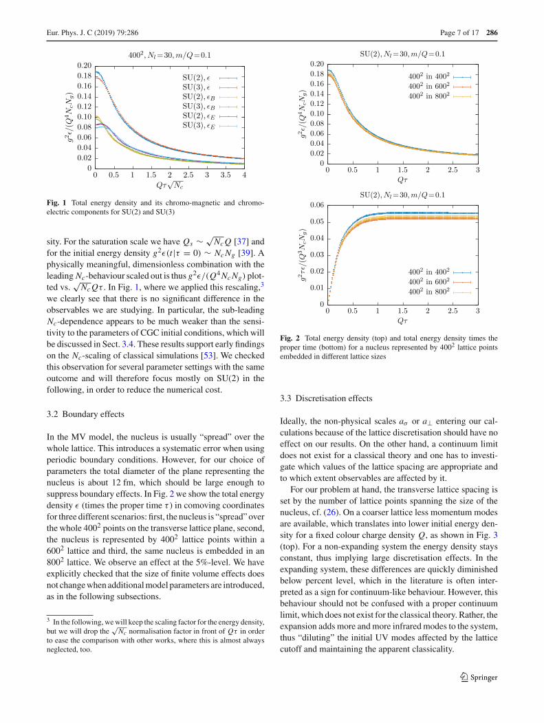
Fig. 1 Total energy density and its chromo-magnetic and chromo-electric components for SU(2) and SU(3)
sity. For the saturation scale we have Qs ∼ √NcQ [37] and
for the initial energy density g2ε(t |τ = 0) ∼ NcNg [39]. Aphysically meaningful, dimensionless combination with theleading Nc-behaviour scaled out is thus g2ε/(Q4NcNg) plot-ted vs.
√NcQτ . In Fig. 1, where we applied this rescaling,3
we clearly see that there is no significant difference in theobservables we are studying. In particular, the sub-leadingNc-dependence appears to be much weaker than the sensi-tivity to the parameters of CGC initial conditions, which willbe discussed in Sect. 3.4. These results support early findingson the Nc-scaling of classical simulations [53]. We checkedthis observation for several parameter settings with the sameoutcome and will therefore focus mostly on SU(2) in thefollowing, in order to reduce the numerical cost.
3.2 Boundary effects
In the MV model, the nucleus is usually “spread” over thewhole lattice. This introduces a systematic error when usingperiodic boundary conditions. However, for our choice ofparameters the total diameter of the plane representing thenucleus is about 12 fm, which should be large enough tosuppress boundary effects. In Fig. 2 we show the total energydensity ε (times the proper time τ ) in comoving coordinatesfor three different scenarios: first, the nucleus is “spread” overthe whole 4002 points on the transverse lattice plane, second,the nucleus is represented by 4002 lattice points within a6002 lattice and third, the same nucleus is embedded in an8002 lattice. We observe an effect at the 5%-level. We haveexplicitly checked that the size of finite volume effects doesnot change when additional model parameters are introduced,as in the following subsections.
3 In the following, we will keep the scaling factor for the energy density,but we will drop the
√Nc normalisation factor in front of Qτ in order
to ease the comparison with other works, where this is almost alwaysneglected, too.
Fig. 2 Total energy density (top) and total energy density times theproper time (bottom) for a nucleus represented by 4002 lattice pointsembedded in different lattice sizes
3.3 Discretisation effects
Ideally, the non-physical scales aσ or a⊥ entering our cal-culations because of the lattice discretisation should have noeffect on our results. On the other hand, a continuum limitdoes not exist for a classical theory and one has to investi-gate which values of the lattice spacing are appropriate andto which extent observables are affected by it.
For our problem at hand, the transverse lattice spacing isset by the number of lattice points spanning the size of thenucleus, cf. (26). On a coarser lattice less momentum modesare available, which translates into lower initial energy den-sity for a fixed colour charge density Q, as shown in Fig. 3(top). For a non-expanding system the energy density staysconstant, thus implying large discretisation effects. In theexpanding system, these differences are quickly diminishedbelow percent level, which in the literature is often inter-preted as a sign for continuum-like behaviour. However, thisbehaviour should not be confused with a proper continuumlimit, which does not exist for the classical theory. Rather, theexpansion adds more and more infrared modes to the system,thus “diluting” the initial UV modes affected by the latticecutoff and maintaining the apparent classicality.
123
286 Page 8 of 17 Eur. Phys. J. C (2019) 79 :286
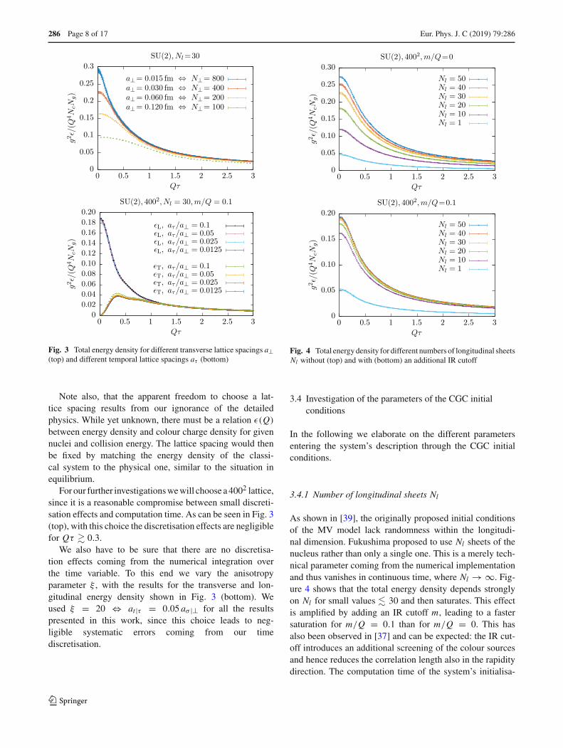
Fig. 3 Total energy density for different transverse lattice spacings a⊥(top) and different temporal lattice spacings aτ (bottom)
Note also, that the apparent freedom to choose a lat-tice spacing results from our ignorance of the detailedphysics. While yet unknown, there must be a relation ε(Q)
between energy density and colour charge density for givennuclei and collision energy. The lattice spacing would thenbe fixed by matching the energy density of the classi-cal system to the physical one, similar to the situation inequilibrium.
For our further investigations we will choose a 4002 lattice,since it is a reasonable compromise between small discreti-sation effects and computation time. As can be seen in Fig. 3(top), with this choice the discretisation effects are negligiblefor Qτ � 0.3.
We also have to be sure that there are no discretisa-tion effects coming from the numerical integration overthe time variable. To this end we vary the anisotropyparameter ξ , with the results for the transverse and lon-gitudinal energy density shown in Fig. 3 (bottom). Weused ξ = 20 ⇔ at |τ = 0.05 aσ |⊥ for all the resultspresented in this work, since this choice leads to neg-ligible systematic errors coming from our timediscretisation.
Fig. 4 Total energy density for different numbers of longitudinal sheetsNl without (top) and with (bottom) an additional IR cutoff
3.4 Investigation of the parameters of the CGC initialconditions
In the following we elaborate on the different parametersentering the system’s description through the CGC initialconditions.
3.4.1 Number of longitudinal sheets Nl
As shown in [39], the originally proposed initial conditionsof the MV model lack randomness within the longitudi-nal dimension. Fukushima proposed to use Nl sheets of thenucleus rather than only a single one. This is a merely tech-nical parameter coming from the numerical implementationand thus vanishes in continuous time, where Nl → ∞. Fig-ure 4 shows that the total energy density depends stronglyon Nl for small values � 30 and then saturates. This effectis amplified by adding an IR cutoff m, leading to a fastersaturation for m/Q = 0.1 than for m/Q = 0. This hasalso been observed in [37] and can be expected: the IR cut-off introduces an additional screening of the colour sourcesand hence reduces the correlation length also in the rapiditydirection. The computation time of the system’s initialisa-
123

Eur. Phys. J. C (2019) 79 :286 Page 9 of 17 286
tion grows linearly with Nl and hence a reasonable choice isNl = 30, which we set for most of our simulations.
3.4.2 IR cutoff m
As explained in the last section, the IR parameterm provides asimple way to incorporate the colour neutrality phenomenonstudied in [54]. While m = 0.1 Q ≈ 1
Rp, with Rp being the
proton radius, is a physically motivated choice, the precisevalue of m/Q has a large effect on the initial energy densitywhich can be seen in Fig. 5 (top). With a higher cutoff, lessmodes are populated to contribute to the energy density. Asstudied in [37], the parameter m also affects the ratio Q/Qs :at Nl = 30 the physical saturation scale Qs is around 0.85 Qfor m/Q = 0.1 and around 1.03 Q for m/Q = 0. Since theenergy density is normalised by Q4, this difference amountsto about a factor of 2 in the dimensionless quantity ε/Q4
s .Since the effect of m is in the infrared, it does not get
washed out by the expansion of the system, in contrast to thediscretisation effects. Hence a careful understanding to fixthis parameter is important. For example, one might won-der whether this inverse length scale should not also beanisotropic in the initial geometry. In what follows we willeither usem = 0, as in the initial MV model, or the physicallymotivated choice m/Q = 0.1.
3.4.3 UV cutoff Λ
As discussed in Sect. 2.2, one can apply a UV cutoff Λ whilesolving Poisson’s equation (20a), in addition to the existinglattice UV cutoff. This is an additional model parameter lim-iting the initial mode population to an infrared sector deter-mined by Λ. Figure 5 (bottom) shows the influence of thisparameter on the energy density, which gets reduced becauseof the missing higher modes in the Poisson equation. This issimilar to the observation we made on the IR cutoff m, butwith the important difference that the ratio Q/Qs is indepen-dent of Λ [55]. We are not aware of a unique argument orprocedure to set this parameter, for the sake of comparisonwith the literature we choose Λ/Q = 1.7 [19] in some ofour later investigations. As a welcome side effect, with theemphasis of the infrared modes strengthened, the dependenceof the total energy density on the lattice spacing is reducedand the expanding system saturates even faster towards a⊥-independent values, cf. Fig. 6 and the previous Fig. 3 (top).
3.5 The energy density mode spectrum
The occupation number of field modes in Fourier space isthe most direct and often applied criterion to judge the valid-ity of the classical approximation during the time evolutionof the system. It is well-established that, starting from CGC
Fig. 5 Total energy density for different IR (top) and UV (bottom)cutoff parameters
Fig. 6 Total energy density for different transverse lattice sizes N 2⊥with an additional UV cutoff of Λ = 1.7 Q
initial conditions, simulations in a static box quickly pop-ulate higher modes, implying a breakdown of the classicaldescription beyond some time. In the expanding system thisprocess is considerably slowed down [19,38,56,57]. We con-firm these earlier findings by plotting our generalised occu-pation number as a function of the momentum modes definedvia (35).
Figure 7 (top) shows the energy mode spectra for differentmodel parameter values at initial time. In order to study the
123

286 Page 10 of 17 Eur. Phys. J. C (2019) 79 :286
Fig. 7 Occupation number as a function of the momentum p/Q atinitial time (top) and after the same number of time steps in the staticbox (middle) and in the expanding formulation (bottom). The highestmomentum is defined by the lattice cutoff, pmax = √
2π/a⊥ ≈ 14.81 Q
full range of the additional UV cutoff, we deliberately choseΛ = Q as its smallest value, cf. (36). One clearly sees that theadditional UV cutoff causes a strong suppression of highermodes, thus strengthening the validity of the classical approx-imation. This is also consistent with the observation fromSect. 3.4.3, that the additional cutoff can be used to weakendiscretisation effects. Another observation is that the distri-bution is rather independent of the IR cutoff value. In Fig. 7
(bottom) we present the evolution of the same initial config-uration in the static and expanding framework. While with-out an additional UV cutoff the distributions nearly reach aplateau in the static box, the occupation of the higher modes inthe expanding system stays considerably lower, thus extend-ing the validity of the classical approximation.
One can now try to get a quantitative measure of thesupposed dominance of infrared modes. By integrating theFourier modes of the energy density up to some momen-tum scale, one can infer the energy fraction of the systemcontained in the modes below that scale, thus assessing theclassicality of the mix (see for example [29]). For exam-ple, without applying any cutoffs, integrating modes up to2Q ≈ 4 GeV contains 65% of the total energy of the systemat initial time. At Qt |Qτ = 150, this changes to 60% or77% in the static and expanding cases, respectively. Hence,the quality of the classical approximation deteriorates onlyslowly or not at all. Nevertheless, a significant systematicerror should be expected when several 10% of the energy isin the UV sector, where a running coupling and other quan-tum effects should be taken into account. This must certainlybe the case when modes � 5Q ≈ 10 GeV get significantlypopulated, as in Fig. 7. At this stage of the evolution a betterdescription might be obtained by an effective kinetic theory[26–28], where quantum effects are already included.
Finally, we remark that the Fourier mode distribution ofenergy density, like occupation number in a free field theory,is also sensitive to the homogeneity of the system in coor-dinate space: a plane wave with only one momentum modeoccupied corresponds to a (finite) delta peak in occupationnumber, whereas wave packets have broader distributions.
3.6 Isotropisation
In this section we add small quantum fluctuations on theinitial conditions, as described by Eq. (25). These initialfluctuations lead to an eventual isotropisation of the system,which can be studied by the evolution of the ratio of thepressure components PL/PT . To include their effects, wehave to extend our two-dimensional analysis by an additionallongitudinal direction Nz|η, increasing the computation timelinearly with Nz|η. Within our computational budget, thisforces us to use smaller lattices (2003) for this section, thusinevitably increasing the cutoff and finite volume effects wehave discussed so far. However, as we shall see, the effectsof the model parameters are by an order of magnitude larger.
3.6.1 Static box
We begin with the static box. The general behaviour of thepressure ratio PL/PT has been known for a while and isshown in Fig. 8. After a peak at around Qt ≈ 0.6 follows anoscillating stage until the system isotropises. The oscillating
123

Eur. Phys. J. C (2019) 79 :286 Page 11 of 17 286
Fig. 8 Pressure ratio in the static box for different longitudinal latticeextents Nz (top) and for different fluctuation amplitudes Δ (bottom)
Table 1 The initial total energy density and its relative increase dueto the fluctuations for different cutoff setups. First row: no additionalcutoff, second row: m/Q = 0.1, third row: m/Q = 0.1 and Λ/Q =1.7. The statistical errors are all below the 1 %-level
g2ε
Q4NcNgRelative increase
Δ = 0 Δ = 10−1 Δ = 10−2 Δ = 10−3
0.163 23.9 % 0.239 % 0.00239 %
0.122 32.2 % 0.321 % 0.00322 %
0.057 68.1 % 0.682 % 0.00683 %
stage originates from turbulent pattern formation and diffu-sion [18,19] and precludes a hydrodynamical description.We see a strong finite size effect in Nz , Fig. 8 (top), whichdecreases for larger values and should vanish in the limitNz → ∞. For very small values of Nz ≤ 10, the fluctuationscannot evolve and the system behaves as in the unperturbedΔ = 0 case.
The dependence on the fluctuation amplitude Δ is studiedin Fig. 8 (bottom). In accord with expectation, increasing thefluctuation amplitude Δ reduces the isotropisation time. Notethe interesting dynamics associated with this: while for largerinitial amplitudes the onset towards isotropisation occurs ear-lier, the eventual growth of the longitudinal pressure appears
Fig. 9 Pressure ratio in the static box for different IR and UV cutoffs(top) and for the different gauge groups (bottom)
Table 2 Hydrodynamisation time extrapolations in units of Q−1 fordifferent lattice and CGC parameter setups
2003 and no additional cutoff
Δ = 10−1 Δ = 10−2 Δ = 10−3
751 770 885
2002 × 20 and Δ = 10−2
No add. Λ/Q = 1.7 m/Q = 0.1 m/Q = 0.1
Cutoff Λ/Q = 1.7
799 1719 3259 4736
to be faster for the smaller amplitudes. The initial fluctuationamplitude Δ also significantly affects the early behaviour ofthe system, causing a strong change of the pressure ratio and asignificant increase of the energy density (∼ Δ2), as shownin Table 1. Also the frequencies of the plasma oscillationsare affected. Of course, increasing the quantum fluctuationamplitude weakens the classicality of the initial condition:for Δ ≥ 0.1 the fluctuations already make up ≥ 20% ofthe initial energy density. On the other hand, for Δ � 10−2
there is no visible effect on the pressure ratio at early times(Qt � 20), and also the energy remains the same withinnumerical fluctuations.
123

286 Page 12 of 17 Eur. Phys. J. C (2019) 79 :286
Fig. 10 Snapshots of thex-component of thechromo-magnetic energydensity in the yz-plane atdifferent times (top down: Qt =0.3, 60, 90, 120, 150, 300) anddifferent fluctuation seeds (leftto right: Δ = 10−1, 10−2, 10−3)
The hydrodynamisation time of a heavy ion collision is thetime, after which hydrodynamics is applicable to describe thedynamics of the system. This is commonly believed to be thecase once the pressure ratio PL/PT ≥ 0.7. For an initialamplitude of Δ = 10−2 and without further model cutoffs,this happens at t ≈ 770/Q ≈ 76 fm in our simulations. Thisvalue is considerably larger than experimentally expected
ones, but it is in line with earlier numerical results in a staticbox, e.g. [19].
The pressure ratio is highly sensitive both to the additionalIR and to the UV cutoff introduced in the initial condition,cf. Fig. 9 (top). Especially the UV cutoff changes the qual-itative shape of the curve at early times significantly. Fur-thermore, both cutoffs considerably slow down the processof isotropisation as shown in Table 2. The hydrodynamisa-
123
Eur. Phys. J. C (2019) 79 :286 Page 13 of 17 286
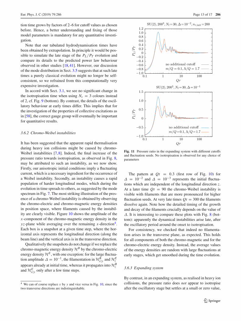
tion time grows by factors of 2–6 for cutoff values as chosenbefore. Hence, a better understanding and fixing of thosemodel parameters is mandatory for any quantitative investi-gation.
Note that our tabulated hydrodynamisation times havebeen obtained by extrapolation. In principle it would be pos-sible to simulate the late stage of the PL/PT evolution andcompare its details to the predicted power law behaviourobserved in other studies [18,41]. However, our discussionof the mode distribution in Sect. 3.5 suggests that at such latetimes a purely classical evolution might no longer be self-consistent, so we refrained from this computationally veryexpensive investigation.
In accord with Sect. 3.1, we see no significant change inthe isotropisation time when using Nc = 3 colours insteadof 2, cf. Fig. 9 (bottom). By contrast, the details of the oscil-latory behaviour at early times differ. This implies that forthe investigation of the properties of collective excitations asin [58], the correct gauge group will eventually be importantfor quantitative results.
3.6.2 Chromo-Weibel instabilities
It has been suggested that the apparent rapid thermalisationduring heavy ion collisions might be caused by chromo-Weibel instabilities [7,8]. Indeed, the final increase of thepressure ratio towards isotropisation, as observed in Fig. 8,may be attributed to such an instability, as we now show.Firstly, our anisotropic initial conditions imply a fluctuatingcurrent, which is a necessary ingredient for the occurrence ofa Weibel instability. Secondly, an instability causes a rapidpopulation of harder longitudinal modes, which during theevolution in time spreads to others, as suggested by the modespectrum in Fig. 7. The most striking illustration of the pres-ence of a chromo-Weibel instability is obtained by observingthe chromo-electric and chromo-magnetic energy densitiesin position space, where filaments caused by the instabil-ity are clearly visible. Figure 10 shows the amplitude of thex-component of the chromo-magnetic energy density in theyz-plane while averaging over the remaining x-direction4.Each box is a snapshot at a given time step, where the hor-izontal axis represents the longitudinal direction (along thebeam line) and the vertical axis is in the transverse direction.
Qualitatively the snapshots do not change if we replace thechromo-magnetic energy density HB by the chromo-electricenergy density HE , with one exception: for the large fluctua-tion amplitude Δ = 10−1, the filamentation in HB
x |y and HEz
appears already at initial time, whereas it propagates intoHBz
and HEx |y only after a few time steps.
4 We can of course replace x by y and vice versa in Fig. 10, since thetwo transverse directions are indistinguishable.
Fig. 11 Pressure ratio in the expanding system with different cutoffsand fluctuation seeds. No isotropisation is observed for any choice ofparameters
The pattern at Qt = 0.3 (first row of Fig. 10) forΔ = 10−2 and Δ = 10−3 represents the initial fluctua-tions which are independent of the longitudinal direction z.At a later time Qt = 90 the chromo-Weibel instability isvisible with filaments that are more pronounced for higherfluctuation seeds. At very late times Qt = 300 the filamentsdissolve again. Note how the detailed timing of the growthand decay of the filaments crucially depends on the value ofΔ. It is interesting to compare these plots with Fig. 8 (bot-tom): apparently the dynamical instabilities arise late, afterthe oscillatory period around the onset to isotropisation.
For consistency, we checked that indeed no filamenta-tion arises in the transverse plane, as expected. This holdsfor all components of both the chromo-magnetic and for thechromo-electric energy density. Instead, the average valuesof the energy densities are random with large fluctuations atearly stages, which get smoothed during the time evolution.
3.6.3 Expanding system
By contrast, in an expanding system, as realised in heavy ioncollisions, the pressure ratio does not appear to isotropiseafter the oscillatory stage but settles at a small or zero value,
123

286 Page 14 of 17 Eur. Phys. J. C (2019) 79 :286
Fig. 12 SU(2) total energy density on a 4002 lattice with Nl = 30 asa function of QL and ΛL at initial time and at Qτ = 0.3. The dashedlines represent constant energy density levels at integer multiples of 108.The red solid lines indicate the constant energy densities correspondingto Λ ∈ {Q, 2Q, 3Q, 4Q} at QL = 120. The yellow solid line refers to
the constant energy density contour obtained for QL = 120 without anadditional UV cutoff, which is the choice of the majority of previousstudies. The gray horizontal line represents the lattice UV cutoff abovewhich the additional UV cutoff no longer affects the system
as shown in Fig. 11. This is in accord with the findings in[14,15,41] and robust under variation of all model param-eters. In particular, it also holds for the largest fluctuationseed considered, cf. Fig. 11 (bottom). Correspondingly, inthe expanding system no dynamic filamentation takes placeeither. Only for fluctuation amplitudes � 10−1 filaments areforced right from the beginning, since the initial configura-tion is equivalent to the one we have shown for the staticbox scenario. The conclusion is that an expanding gluonicsystem dominated by classical fields according to the CGCdoes not appear to isotropise and thermalise. For future workit would now be interesting to check whether adding lightquark degrees of freedom helps towards thermalisation, asone might expect.
Note that the non-thermalisation of the expanding classi-cal system is in marked contrast to simulations of an effec-tive kinetic theory, which predict hydrodynamisation times
consistent with phenomenological expectations [28,59] (see,however, [23]). Further studies of the systematics of bothapproaches are necessary to see whether quantum effectsand/or the role of the UV sector are the reason for this dis-crepancy.
3.7 Initial condition at fixed energy density
Altogether the numerical results of classical simulationsshow a large dependence on the various model parameters ofthe CGC initial condition. This creates a difficult situation,because the initial condition and the early stages of the evolu-tion until freeze-out are so far not accessible experimentally.We now propose a different analysis of the simulation datawhich should be useful in constraining model parameterssuch as Λ,m and Δ.
123

Eur. Phys. J. C (2019) 79 :286 Page 15 of 17 286
Fig. 13 Total energy density for different fluctuation seeds Δ and dif-ferent UV cutoffs Λ/Q at initial time. The dashed lines represent con-stant energy density levels in multiples of 0.025. The solid green linecorresponds to the energy density obtained without an additional UVcutoff and no fluctuations, i.e. Δ = 0. The horizontal grey line repre-sents the lattice cutoff above which the additional cutoff Λ no longeraffects the system
In a physical heavy ion collision the initial state is char-acterised by a colour charge density, an energy density andsome effective values of Λ,m and Δ. However, these cannotall be independent, rather we must have ε = ε(Q,Λ, . . .),where the detailed relation is fixed by the type of nucleiand their collision energy. We should thus analyse computa-tions with fixed initial energy density L4ε, while varying themodel parameters. The outcome of such an investigation forΛ and Q are the contour plots shown in Fig. 12. We considerQτ = 0.3 as well, since then even without an additional UVcutoff the discretisation effects are negligible for N⊥ = 400,cf. Fig. 3. In the same figure we also compare the situationwith an additional IR cutoff as discussed earlier. Thus, tothe extent that the energy density as a function of time canbe determined experimentally, it should be possible to estab-lish relations between the parameters Q,Λ and m to furtherconstrain the initial state.
The same consideration can be applied to study the fluc-tuation amplitude. Figure 13 shows contours of fixed energydensity ε/Q4 in the (Δ,Λ/Q) plane, where Δ = 0 repre-sents the classical MV initial conditions, i.e., the tree-levelCGC description without any quantum fluctuations, and wehave chosen QL = 120. Clearly, similar studies can be madefor any pairing of the model parameters at any desired timeduring the evolution and should help in establishing relationsbetween them in order to constrain the initial conditions.
4 Conclusions
We presented a systematic investigation of the dependenceof the energy density and the pressure on the parameters
entering the lattice description of classical Yang–Mills the-ory, starting from the CGC initial conditions. This was donein a static box framework as well as in an expanding geometryand both for Nc = 2 and Nc = 3 colours.
After the leading Nc-dependence is factored out, devia-tions between the SU(2) and the SU(3) formulation are smalland only visible in the details of the evolution during the earlyturbulent stage. This is not surprising in a classical treatment,since in the language of Feynman diagrams most of the sub-leading Nc-behaviour is contained in loop, i.e. quantum, cor-rections.
Finite volume effects are related to the treatment of theboundary of the colliding nuclei and their embedding on thelattice. Given sizes of ∼ 10 fm, such effects are at a mild 5%-level. Note, however, that this effect is larger than the finitesize effects of the same box on the vacuum hadron spectrum,as expected for a many-particle problem.
The choice of the lattice spacing affects the number ofmodes available in the field theory and thus significantlyinfluences the relation between the initial colour distributionand the total energy of the system. In the static box, all furtherevolution is naturally affected by this. Since the classical the-ory has no continuum limit, the lattice spacing would need tobe fixed by some matching condition at the initial stage. Bycontrast, in the expanding system the energy density quicklydiminishes and the effect of the lattice spacing is washed out.
A quantitatively much larger and significant role is playedby the model parameters of the initial conditions, specifi-cally additional IR and UV cutoffs affecting the distributionof modes and the amplitude of initial quantum fluctuations,whose presence is a necessary condition for isotropisation.For the static box we presented direct evidence for isotropi-sation to proceed through the emergence of chromo-Weibelinstabilities, which are clearly visible as filamentation ofthe energy density. However, the hydrodynamisation timeis unphysically large and gets increased further by additionalIR- and UV-cutoffs in the initial condition. Without quan-titative knowledge of these parameters, the hydrodynami-sation time varies within a factor of five. We suggested amethod to study the parameters’ influence on the system atconstant initial energy densities. This allows to establish rela-tions between different parameter sets that should be usefulto constrain their values.
Rather strikingly, no combination of model parametersleads to isotropisation in the expanding classical gluonic sys-tem.
Acknowledgements We thank K. Fukushima, J. Glesaaen, M. Greif,H. van Hees, A. Mazeliauskas, P. Romatschke, B. Schenke, J. Sche-unert, S. Schlichting and R. Venugopalan for useful discussions. Weare grateful to M. Attems and C. Schaefer for collaboration during theinitial stages of this project and to FUCHS- and LOEWE-CSC high-performance computers of the Frankfurt University for providing com-putational resources. O.P. and B.W. are supported by the Helmholtz
123

286 Page 16 of 17 Eur. Phys. J. C (2019) 79 :286
International Center for FAIR within the framework of the LOEWEprogram launched by the State of Hesse. S.Z. acknowledges support bythe DFG Collaborative Research Centre SFB 1225 (ISOQUANT).
Data Availability Statement This manuscript has associated data ina data repository. [Author’s comment: This is a theoretical work, noexperimental data were used.]
Open Access This article is distributed under the terms of the CreativeCommons Attribution 4.0 International License (http://creativecommons.org/licenses/by/4.0/), which permits unrestricted use, distribution,and reproduction in any medium, provided you give appropriate creditto the original author(s) and the source, provide a link to the CreativeCommons license, and indicate if changes were made.Funded by SCOAP3.
References
1. U.W. Heinz, P.F. Kolb, Early thermalization at RHIC. Nucl. Phys.A 702, 269–280 (2002). arXiv:hep-ph/0111075 [hep-ph]
2. P. Romatschke, U. Romatschke, Viscosity information from rel-ativistic nuclear collisions: how perfect is the fluid observed atRHIC? Phys. Rev. Lett. 99, 172301 (2007). arXiv:0706.1522 [nucl-th]
3. P. Romatschke, Do nuclear collisions create a locally equili-brated quarkâASgluon plasma? Eur. Phys. J. C 77(1), 21 (2017).arXiv:1609.02820 [nucl-th]
4. E. Iancu, A. Leonidov, L.D. McLerran, Nonlinear gluon evolu-tion in the color glass condensate. 1. Nucl. Phys. A 692, 583–645(2001). arXiv:hep-ph/0011241 [hep-ph]
5. P.F. Kolb, J. Sollfrank, U.W. Heinz, Anisotropic transverse flowand the quark hadron phase transition. Phys. Rev. C 62, 054909(2000). arXiv:hep-ph/0006129 [hep-ph]
6. U.W. Heinz, Quark–gluon transport theory. Nucl. Phys. A 418,603C–612C (1984)
7. S. Mrowczynski, Stream instabilities of the quark–gluon plasma.Phys. Lett. B 214, 587 (1988)
8. Y. Pokrovsky, A. Selikhov, Filamentation in a quark–gluon plasma.JETP Lett. 47, 12–14 (1988)
9. S. Mrowczynski, Plasma instability at the initial stage of ultrarel-ativistic heavy ion collisions. Phys. Lett. B 314, 118–121 (1993)
10. J.-P. Blaizot, E. Iancu, The quark gluon plasma: collective dynam-ics and hard thermal loops. Phys. Rep. 359, 355–528 (2002).arXiv:hep-ph/0101103 [hep-ph]
11. P. Romatschke, M. Strickland, Collective modes of an anisotropicquark gluon plasma. Phys. Rev. D 68, 036004 (2003).arXiv:hep-ph/0304092 [hep-ph]
12. P.B. Arnold, J. Lenaghan, G.D. Moore, QCD plasma instabil-ities and bottom up thermalization. JHEP 0308, 002 (2003).arXiv:hep-ph/0307325 [hep-ph]
13. M.E. Carrington, K. Deja, S. Mrowczynski, Plasmons inanisotropic quark–gluon plasma. Phys. Rev. C 90, 034913 (2014).arXiv:1407.2764 [hep-ph]
14. P. Romatschke, R. Venugopalan, Collective non-Abelian instabili-ties in a melting color glass condensate. Phys. Rev. Lett. 96, 062302(2006). arXiv:hep-ph/0510121 [hep-ph]
15. P. Romatschke, R. Venugopalan, The unstable glasma. Phys. Rev.D 74, 045011 (2006). arXiv:hep-ph/0605045 [hep-ph]
16. K. Fukushima, Evolving Glasma and Kolmogorov spectrum. ActaPhys. Polon. B 42, 2697–2715 (2011). arXiv:1111.1025 [hep-ph]
17. J. Berges, K. Boguslavski, S. Schlichting, Nonlinear amplifica-tion of instabilities with longitudinal expansion. Phys. Rev. D 85,076005 (2012). arXiv:1201.3582 [hep-ph]
18. J. Berges, K. Boguslavski, S. Schlichting, R. Venugopalan, Tur-bulent thermalization process in heavy-ion collisions at ultrarela-tivistic energies. Phys. Rev. D 89, 074011 (2014). arXiv:1303.5650[hep-ph]
19. K. Fukushima, Turbulent pattern formation and diffusion in theearly-time dynamics in relativistic heavy-ion collisions. Phys. Rev.C 89(2), 024907 (2014). arXiv:1307.1046 [hep-ph]
20. F. Gelis, Color glass condensate and glasma. Int. J. Mod. Phys. A28, 1330001 (2013). arXiv:1211.3327 [hep-ph]
21. A. Kurkela, G.D. Moore, Thermalization in weakly coupled non-abelian plasmas. JHEP 1112, 044 (2011). arXiv:1107.5050 [hep-ph]
22. A. Kurkela, G.D. Moore, Bjorken flow, plasma instabilities, andthermalization. JHEP 1111, 120 (2011). arXiv:1108.4684 [hep-ph]
23. P. Romatschke, A. Rebhan, Plasma instabilities in an anisotrop-ically expanding geometry. Phys. Rev. Lett. 97, 252301 (2006).arXiv:hep-ph/0605064 [hep-ph]
24. A. Rebhan, M. Strickland, M. Attems, Instabilities of an anisotropi-cally expanding non-Abelian plasma: 1D+3V discretized hard-loopsimulations. Phys. Rev. D 78, 045023 (2008). arXiv:0802.1714[hep-ph]
25. M. Attems, A. Rebhan, M. Strickland, Instabilities of an anisotropi-cally expanding non-Abelian plasma: 3D+3V discretized hard-loopsimulations. Phys. Rev. D 87, 025010 (2013). arXiv:1207.5795[hep-ph]
26. R. Baier, A.H. Mueller, D. Schiff, D.T. Son, ’Bottom up’ thermal-ization in heavy ion collisions. Phys. Lett. B 502, 51–58 (2001).arXiv:hep-ph/0009237 [hep-ph]
27. P.B. Arnold, G.D. Moore, L.G. Yaffe, Effective kinetic the-ory for high temperature gauge theories. JHEP 01, 030 (2003).arXiv:hep-ph/0209353 [hep-ph]
28. A. Kurkela, Initial state of heavy-ion collisions: isotropiza-tion and thermalization. Nucl. Phys. A 956, 136–143 (2016).arXiv:1601.03283 [hep-ph]
29. J. Berges, K. Boguslavski, S. Schlichting, R. Venugopalan, Basinof attraction for turbulent thermalization and the range of valid-ity of classical–statistical simulations. JHEP 05, 054 (2014).arXiv:1312.5216 [hep-ph]
30. G. Aarts, J. Berges, Classical aspects of quantum fieldsfar from equilibrium. Phys. Rev. Lett. 88, 041603 (2002).arXiv:hep-ph/0107129 [hep-ph]
31. A.H. Mueller, D.T. Son, On the equivalence between the Boltzmannequation and classical field theory at large occupation numbers.Phys. Lett. B 582, 279–287 (2004). arXiv:hep-ph/0212198 [hep-ph]
32. S. Jeon, The Boltzmann equation in classical and quantum fieldtheory. Phys. Rev. C 72, 014907 (2005). arXiv:hep-ph/0412121[hep-ph]
33. M. Attems, O. Philipsen, C. Schäfer, B. Wagenbach, S. Zafeiropou-los, A real-time lattice simulation of the thermalization of a gluonplasma: first results. Acta Phys. Polon. Suppl. 9, 603 (2016).arXiv:1605.07064 [hep-ph]
34. L.D. McLerran, The color glass condensate and small xphysics: four lectures. Lect. Notes Phys. 583, 291–334 (2002).arXiv:hep-ph/0104285 [hep-ph]
35. E. Iancu, R. Venugopalan, The color glass condensate and high-energy scattering in QCD. arXiv:hep-ph/0303204 [hep-ph]
36. L.D. McLerran, R. Venugopalan, Gluon distribution functions forvery large nuclei at small transverse momentum. Phys. Rev. D 49,3352–3355 (1994). arXiv:hep-ph/9311205 [hep-ph]
37. T. Lappi, Wilson line correlator in the MV model: relating theglasma to deep inelastic scattering. Eur. Phys. J. C 55, 285–292(2008). arXiv:0711.3039 [hep-ph]
38. H. Fujii, K. Fukushima, Y. Hidaka, Initial energy density and gluondistribution from the Glasma in heavy-ion collisions. Phys. Rev. C79, 024909 (2009). arXiv:0811.0437 [hep-ph]
123

Eur. Phys. J. C (2019) 79 :286 Page 17 of 17 286
39. K. Fukushima, Randomness in infinitesimal extent in theMcLerran–Venugopalan model. Phys. Rev. D 77, 074005 (2008).arXiv:0711.2364 [hep-ph]
40. A. Kurkela, G.D. Moore, UV cascade in classical Yang–Mills the-ory. Phys. Rev. D 86, 056008 (2012). arXiv:1207.1663 [hep-ph]
41. J. Berges, K. Boguslavski, S. Schlichting, R. Venugopalan, Univer-sal attractor in a highly occupied non-Abelian plasma. Phys. Rev.D 89(11), 114007 (2014). arXiv:1311.3005 [hep-ph]
42. B. Gough, GNU Scientific Library Reference Manual, 3rd edn.(Network Theory Ltd., Massachusetts, 2009)
43. K. Fukushima, F. Gelis, L. McLerran, Initial singularity of the littlebang. Nucl. Phys. A 786, 107–130 (2007). arXiv:hep-ph/0610416[hep-ph]
44. T. Epelbaum, F. Gelis, Fluctuations of the initial color fields inhigh energy heavy ion collisions. Phys. Rev. D 88, 085015 (2013).arXiv:1307.1765 [hep-ph]
45. K. Fukushima, F. Gelis, The evolving Glasma. Nucl. Phys. A 874,108–129 (2012). arXiv:1106.1396 [hep-ph]
46. T. Lappi, L. McLerran, Some features of the glasma. Nucl. Phys.A 772, 200–212 (2006). arXiv:hep-ph/0602189 [hep-ph]
47. A. Krasnitz, R. Venugopalan, The Initial gluon multiplicity inheavy ion collisions. Phys. Rev. Lett. 86, 1717–1720 (2001).arXiv:hep-ph/0007108 [hep-ph]
48. T. Lappi, Production of gluons in the classical field modelfor heavy ion collisions. Phys. Rev. C 67, 054903 (2003).arXiv:hep-ph/0303076 [hep-ph]
49. D. Bodeker, K. Rummukainen, Non-abelian plasma instabilities forstrong anisotropy. JHEP 07, 022 (2007). arXiv:0705.0180 [hep-ph]
50. J.P. Blaizot, T. Lappi, Y. Mehtar-Tani, On the gluon spectrum inthe glasma. Nucl. Phys. A 846, 63–82 (2010). arXiv:1005.0955[hep-ph]
51. G.D. Moore, Problems with lattice methods for electroweak pre-heating. JHEP 11, 021 (2001). arXiv:hep-ph/0109206 [hep-ph]
52. SciDAC Collaboration, LHPC Collaboration, UKQCD Collabora-tion Collaboration, R.G. Edwards, B. Joo, The Chroma softwaresystem for lattice QCD. Nucl. Phys. Proc. Suppl.140, 832 (2005).arXiv:hep-lat/0409003 [hep-lat]
53. A. Ipp, A. Rebhan, M. Strickland, Non-Abelian plasma insta-bilities: SU(3) vs. SU(2). Phys.Rev. D84, 056003 (2011).arXiv:1012.0298 [hep-ph]
54. E. Iancu, K. Itakura, L. McLerran, A Gaussian effective the-ory for gluon saturation. Nucl. Phys. A 724, 181–222 (2003).arXiv:hep-ph/0212123 [hep-ph]
55. R.J. Fries, J.I. Kapusta, Y. Li, Near-fields and initial energy densityin the color glass condensate model. arXiv:nucl-th/0604054 [nucl-th]
56. Y.V. Kovchegov, Can thermalization in heavy ion collisions bedescribed by QCD diagrams? Nucl. Phys. A 762, 298–325 (2005)
57. T. Lappi, Energy density of the glasma. Phys. Lett. B 643, 11–16(2006). arXiv:hep-ph/0606207 [hep-ph]
58. K. Boguslavski, A. Kurkela, T. Lappi, J. Peuron, Spectral functionfor overoccupied gluodynamics from real-time lattice simulations.Phys. Rev. D 98(1), 014006 (2018). arXiv:1804.01966 [hep-ph]
59. A. Kurkela, Y. Zhu, Isotropization and hydrodynamization inweakly coupled heavy-ion collisions. Phys. Rev. Lett. 115(18),182301 (2015). arXiv:1506.06647 [hep-ph]
123