From Surface To Objects: Computer Vision

and Three Dimensional Scene Analysis

Robert B. Fisher

This book was originally published by John Wiley and Sons,Chichester, 1989.

PREFACE

Three dimensional scene analysis has reached a turning point. Though re-searchers have been investigating object recognition and scene understandingsince the late 1960’s, a new excitement can be felt in the field. I attributethis to four converging activities: (1) the increasing popularity and suc-cesses of stereo and active range sensing systems, (2) the set of emergingtools and competences concerned with three dimensional surface shape andits meaningful segmentation and description, (3) Marr’s attempt to placethree dimensional vision into a more integrated and scientific context and(4) Brooks’ demonstration of what a more intelligent three dimensional sceneunderstander might entail. It is the convergence of these that has led to theproblem considered in this book: “Assuming that we have easily accessiblesurface data and can segment it into useful patches, what can we then dowith it?”. The work presented here takes an integrated view of the problemsand demonstrates that recognition can actually be done.

The central message of this book is that surface information can greatlysimplify the image understanding process. This is because surfaces are thefeatures that directly link perception to the objects perceived (for normal“camera-like” sensing) and because they make explicit information neededto understand and cope with some visual problems (e.g. obscured features).

Hence, this book is as much about a style of model-based three dimen-sional scene analysis as about a particular example of that style. That stylecombines surface patches segmented from the three dimensional scene de-scription, surface patch based object models, a hierarchy of representations,models and recognitions, a distributed network-based model invocation pro-cess, and a knowledge-based model matcher. Part of what I have tried to dowas show that these elements really do fit together well – they make it easy toextend the competence of current vision systems without extraordinary com-plications, and don’t we all know how fragile complicated computer-based

i

ii

processes are?This book is an organic entity – the research described started in 1982

and earlier results were reported in a PhD thesis in 1985. Since then, re-search has continued under the United Kingdom Alvey program, replacingweak results and extending into new areas, and most of the new results areincluded here. Some of the processes are still fairly simple and need furtherdevelopment, particularly when working with automatically segmented data.Thus, this book is really just a “progress report” and its content will continueto evolve. In a way, I hope that I will be able to rewrite the book in five to tenyears, reporting that all problems have been solved by the computer visioncommunity and showing that generic three dimensional object recognitioncan now be done. Who knows?

The book divides naturally into three parts. Chapters three to six de-scribe the model independent scene analysis. The middle chapters, sevenand eight, describe how objects are represented and selected, and thus howone can pass from an iconic to a symbolic scene representation. The finalchapters then describe our approach to geometric model-based vision – howto locate, verify and understand a known object given its geometric model.

There are many people I would like to thank for their help with the workand the book. Each year there are a few more people I have had the pleasureof working and sharing ideas with. I feel awkward about ranking people bythe amount or the quality of the help given, so I will not do that. I wouldrather bring them all together for a party (and if enough people buy thisbook I’ll be able to afford it). The people who would be invited to the partyare: (for academic advice) Damal Arvind, Jon Aylett, Bob Beattie, Li DongCai, Mike Cameron-Jones, Wayne Caplinger, John Hallam, David Hogg, JimHowe, Howard Hughes, Zi Qing Li, Mark Orr, Ben Paechter, Fritz Seytter,Manuel Trucco, (and for help with the materials) Paul Brna, Douglas Howie,Doug Ramm, David Robertson, Julian Smart, Lincoln Wallen and DavidWyse and, of course, Gaynor Redvers-Mutton and the staff at John Wiley &Sons, Ltd. for their confidence and support.

Well, I take it back. I would particularly like to thank Mies for her love,support and assistance. I’d also like to thank the University of Edinburgh, theAlvey Programme, my mother and Jeff Mallory for their financial support,without which this work could not have been completed.

Bob Fisher 1989PostscriptWith the advances in technology, I am pleased to now add the book to the

iii

web. Much of the content is a bit dated; however I think that the sections on:Making Complete Surface Hypotheses (Chapter 4), Surface Clusters (Chap-ter 5), Model Invocation (Chapter 8), Feature Visibility Analysis (Section9.3) and Binding Subcomponents with Degrees of Freedom (Section 9.4.4)still have something offer researchers.

In addition, it may be interesting for beginning researchers as a more-or-less complete story, rather than the compressed view that you get in confer-ence and journal papers.

I offer many thanks to Anne-Laure Cromphout who helped with thepreparation of this web version.

Bob Fisher March 2004

Chapter 1

An Introduction to RecognitionUsing Surfaces

The surface is the boundary between object and non-object and is the usualsource and limit of perception. As such, it is the feature that unifies mostsignificant forms of non-invasive sensing, including the optical, sonar, radarand tactile modalities in both active and passive forms. The presence of thesurface (including its location) is the primary fact. Perceived intensity issecondary – it informs on the appearance of the surface as seen by the viewerand is affected by the illumination and the composition of the surface.

Grimson, in his celebrated book “From Images to Surfaces: A Compu-tational Study of the Human Early Visual System” [77], described an ele-gant approach to constructing a surface representation of a scene, startingfrom a stereo pair of intensity images. The approach, based substantially onMarr’s ideas [112], triangulated paired image features (e.g. edge fragments)to produce a sparse depth image, and then reconstructed a complete surface,giving a dense depth image. Though this is not the only way to acquire sucha surface description, (e.g. laser ranging and structured light are practicalalternatives), there have been only a few attempts at exploiting this rich datafor object recognition.

Previous research in object recognition has developed theories for recog-nizing simple objects completely, or complex objects incompletely. With theknowledge of the “visible” surfaces of the scene, the complete identificationand location of more complex objects can be inferred and verified, whichis the topic of this book. Starting from a full surface representation, wewill look at new approaches to making the transformation from surfaces to

1

2

objects. The main results, as implemented in the IMAGINE I program,are:

• Surface information directly provides three dimensional cues for surfacegrouping, leading to a volumetric description of the objects in the scene.

• Structural properties can be directly estimated from the three dimen-sional data, rather than from two dimensional projections.

• These properties plus the generic and structural relationships in themodel base can be used to directly invoke models to explain the data.

• Using surfaces as both the model and data primitive allows direct pre-diction of visibility relationships, surface matching, prediction and anal-ysis of occlusion and verification of identity.

• Moderately complex non-rigidly connected structures can be thoroughlyrecognized, spatially located and verified.

1.1 Object Recognition

The following definition is proposed:

Three dimensional object recognition is the identification of amodel structure with a set of image data, such that geometricallyconsistent model-to-data correspondences are established and theobject’s three dimensional scene position is known. All model fea-tures should be fully accounted for – by having consistent imageevidence either supporting their presence or explaining their ab-sence.

Hence, recognition produces a symbolic assertion about an object, itslocation and the use of image features as evidence. The matched featuresmust have the correct types, be in the right places and belong to a single,distinct object. Otherwise, though the data might resemble those from theobject, the object is improperly assumed and is not at the proposed location.

Traditional object recognition programs satisfy weaker versions of theabove definition. The most common simplification comes from the assump-tion of a small, well-characterized, object domain. There, identification canbe achieved via discrimination using simply measured image features, such

3

as object color or two dimensional perimeter or the position of a few linearfeatures. This is identification, but not true recognition (i.e. image under-standing).

Recognition based on direct comparison between two dimensional imageand model structures – notably through matching boundary sections – hasbeen successful with both grey scale and binary images of flat, isolated,moderately complicated industrial parts. It is simple, allowing geometricpredictions and derivations of object location and orientation and toleratinga limited amount of noise. This method is a true recognition of the objects –all features of the model are accounted for and the object’s spatial locationis determined.

Some research has started on recognizing three dimensional objects, butwith less success. Model edges have been matched to image edges (withboth two and three dimensional data) while simultaneously extracting theposition parameters of the modeled objects. In polyhedral scenes, recognitionis generally complete, but otherwise only a few features are found. The limitsof the edge-based approach are fourfold:

1. It is hard to get reliable, repeatable and accurate edge information froman intensity image.

2. There is much ambiguity in the interpretation of edge features as shadow,reflectance, orientation, highlight or obscuring edges.

3. The amount of edge information present in a realistic intensity imageis overwhelming and largely unorganizable for matching, given currenttheories.

4. The edge-based model is too simple to deal with scenes involving curvedsurfaces.

Because of these deficiencies, model-based vision has started to exploit thericher information available in surface data.

Surface Data

In the last decade, low-level vision research has been working towardsdirect deduction and representation of scene properties – notably surface

4

depth and orientation. The sources include stereo, optical flow, laser orsonar range finding, surface shading, surface or image contours and variousforms of structured lighting.

The most well-developed of the surface representations is the 212D sketch

advocated by Marr [112]. The sketch represents local depth and orientationfor the surfaces, and labels detected surface boundaries as being from shapeor depth discontinuities. The exact details of this representation and its ac-quisition are still being researched, but its advantages seem clear enough.Results suggest that surface information reduces data complexity and inter-pretation ambiguity, while increasing the structural matching information.

The richness of the data in a surface representation, as well as its immi-nent availability, offers hope for real advances beyond the current practicalunderstanding of largely polyhedral scenes. Distance, orientation and imagegeometry enable a reasonable reconstruction of the three dimensional shapeof the object’s visible surfaces, and the boundaries lead to a figure/groundseparation. Because it is possible to segment and characterize the surfaces,more compact symbolic representations are feasible. These symbolic struc-tures have the same relation to the surface information as edges currently doto intensity information, except that their scene interpretation is unambigu-ous. If there were:

• reasonable criteria for segmenting both the image surfaces and models,

• simple processes for selecting the models and relating them to the dataand

• an understanding of how all these must be modified to account forfactors in realistic scenes (including occlusion)

then object recognition could make significant advances.

The Research Undertaken

The goal of object recognition, as defined above, is the complete matchingof model to image structures, with the concomitant extraction of positioninformation. Hence, the output of recognition is a set of fully instantiatedor explained object hypotheses positioned in three dimensions, which aresuitable for reconstructing the object’s appearance.

5

The research described here tried to attain these goals for moderatelycomplex scenes containing multiple self-obscuring objects. To fully recognizethe objects, it was necessary to develop criteria and practical methods for:

• piecing together surfaces fragmented by occlusion,

• grouping surfaces into volumes that might be identifiable objects,

• describing properties of three dimensional structures,

• selecting models from a moderately sized model base,

• pairing model features to data features and extracting position esti-mates and

• predicting and verifying the absence of model features because of vari-ations of viewpoint.

The approach requires object models composed of a set of surfaces ge-ometrically related in three dimensions (either directly or through subcom-ponents). For each model SURFACE, recognition finds those image surfacesthat consistently match it, or evidence for their absence (e.g. obscuring struc-ture). The model and image surfaces must agree in location and orientation,and have about the same shape and size, with variations allowed for partiallyobscured surfaces. When surfaces are completely obscured, evidence for theirexistence comes either from predicting self-occlusion from the location andorientation of the model, or from finding closer, unrelated obscuring surfaces.

The object representation requires the complete object surface to be seg-mentable into what would intuitively be considered distinct surface regions.These are what will now be generally called surfaces (except where there isconfusion with the whole object’s surface). When considering a cube, thesix faces are logical candidates for the surfaces; unfortunately, most naturalstructures are not so simple. The segmentation assumption presumes thatthe object can be decomposed into rigid substructures (though possibly non-rigidly joined), and that the rigid substructures can be uniquely segmentedinto surfaces of roughly constant character, defined by their two principalcurvatures. It is also assumed that the image surfaces will segment in corre-spondence with the model SURFACEs, though if the segmentation criteria isobject-based, then the model and data segmentations should be similar. (TheSURFACE is the primitive model feature, and represents a surface patch.)

6

Of course, these assumptions are simplistic because surface deformation andobject variations lead to alternative segmentations, but a start must be madesomewhere.

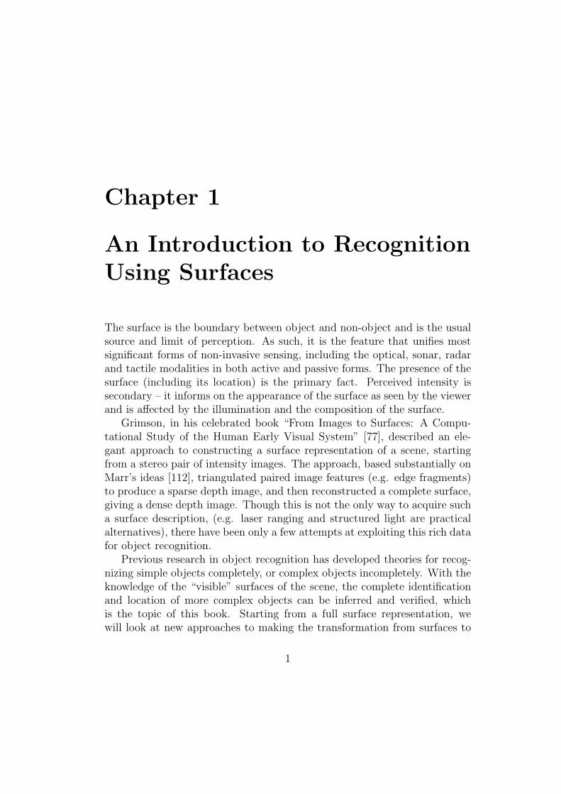
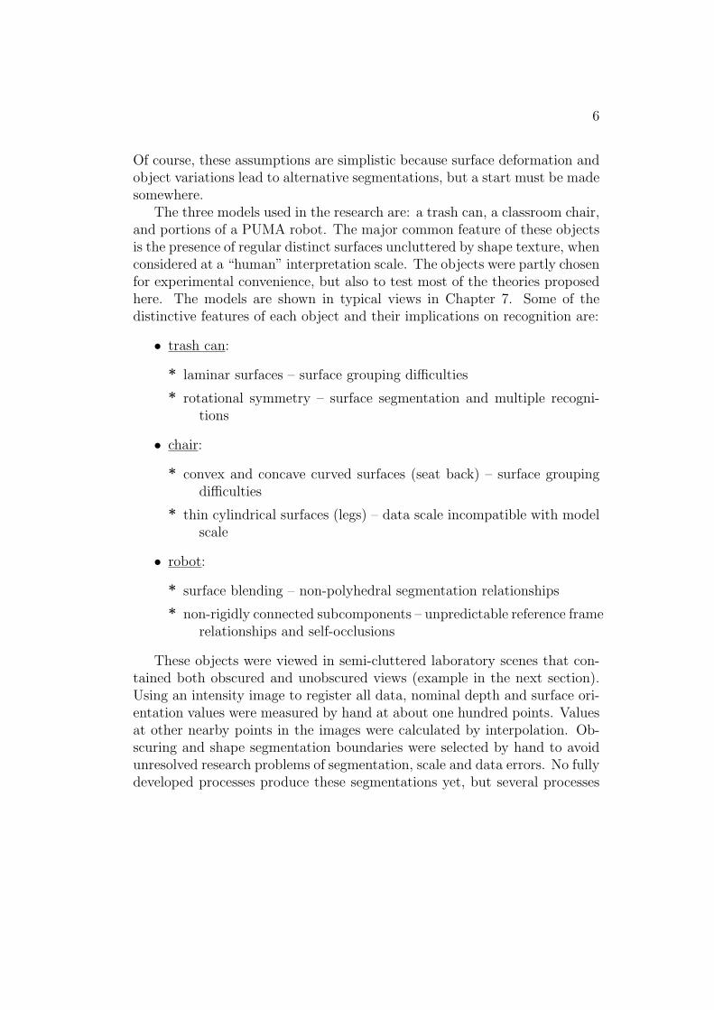
The three models used in the research are: a trash can, a classroom chair,and portions of a PUMA robot. The major common feature of these objectsis the presence of regular distinct surfaces uncluttered by shape texture, whenconsidered at a “human” interpretation scale. The objects were partly chosenfor experimental convenience, but also to test most of the theories proposedhere. The models are shown in typical views in Chapter 7. Some of thedistinctive features of each object and their implications on recognition are:

• trash can:

* laminar surfaces – surface grouping difficulties

* rotational symmetry – surface segmentation and multiple recogni-tions

• chair:

* convex and concave curved surfaces (seat back) – surface groupingdifficulties

* thin cylindrical surfaces (legs) – data scale incompatible with modelscale

• robot:

* surface blending – non-polyhedral segmentation relationships

* non-rigidly connected subcomponents – unpredictable reference framerelationships and self-occlusions

These objects were viewed in semi-cluttered laboratory scenes that con-tained both obscured and unobscured views (example in the next section).Using an intensity image to register all data, nominal depth and surface ori-entation values were measured by hand at about one hundred points. Valuesat other nearby points in the images were calculated by interpolation. Ob-scuring and shape segmentation boundaries were selected by hand to avoidunresolved research problems of segmentation, scale and data errors. No fullydeveloped processes produce these segmentations yet, but several processes

7

are likely to produce them data in the near future and assuming such seg-mentations were possible to allowed us to concentrate on the primary issuesof representation and recognition.

1.2 An Overview of the Research

This section summarizes the work discussed in the rest of the book by pre-senting an example of IMAGINE I’s surface-based object recognition [68].The test image discussed in the following example is shown in Figure 1.1.The key features of the scene include:

• variety of surface shapes and curvature classes,

• solids connected with rotational degrees-of-freedom,

• partially and completely self-obscured structure,

• externally obscured structure,

• structure broken up by occlusion and

• intermingled objects.

Recognition is based on comparing observed and deduced properties withthose of a prototypical model. This definition immediately introduces fivesubtasks for the complete recognition process:

• finding the structures that have the properties,

• acquiring the data properties,

• selecting a model for comparison,

• comparing the data with the model structures and properties, and

• discovering or justifying any missing structures.

The deduction process needs the location and orientation of the objectto predict obscured structures and their properties, so this adds:

• estimating the object’s location and orientation.

8

Figure 1.1: Test Scene

9

This, in turn, is based on inverting the geometric relationships between dataand model structures, which adds:

• making model-to-data correspondences.

The remainder of this section elaborates on the processes and the dataflow dependencies that constrain their mutual relationship in the completerecognition computation context. Figure 1.2 shows the process sequence de-termined by the constraints, and is discussed in more detail below.

Surface Image Inputs

Recognition starts from surface data, as represented in a structure calleda labeled, segmented surface image (Chapter 3). This structure is like Marr’s21

2D sketch and includes a pointillistic representation of absolute depth and

local surface orientation.Data segmentation and organization are both difficult and important.

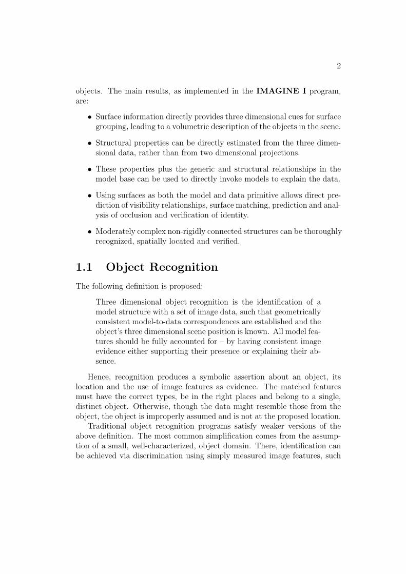
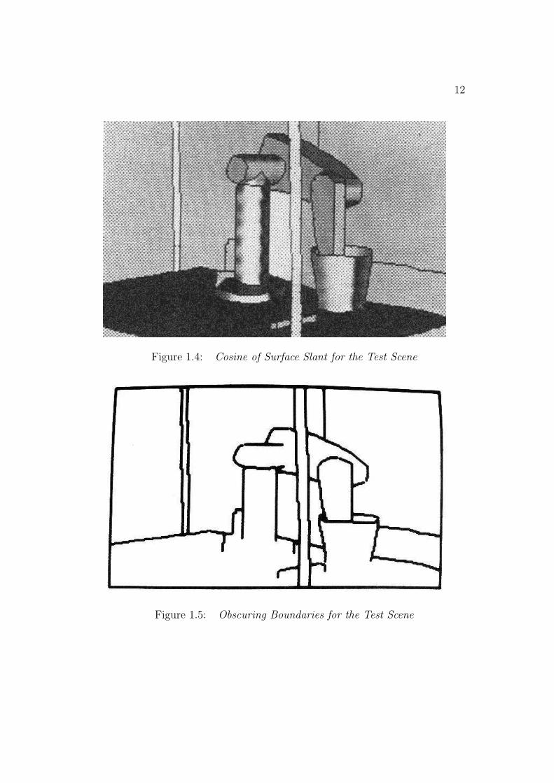
Their primary justifications are that segmentation highlights the relevantfeatures for the rest of the recognition process and organization produces, ina sense, a figure/ground separation. Properties between unrelated structureshould not be computed, such as the angle between surface patches on sep-arate objects. Otherwise, coincidences will invoke and possibly substantiatenon-existent objects. Here, the raw data is segmented into regions by bound-ary segments labeled as shape or obscuring. Shape segmentation is basedon orientation, curvature magnitude and curvature direction discontinuities.Obscuring boundaries are placed at depth discontinuities. These criteria seg-ment the surface image into regions of nearly uniform shape, characterizedby the two principal curvatures and the surface boundary. As no fully devel-oped processes produce this data yet, the example input is from a computeraugmented, hand-segmented test image. The segmentation boundaries werefound by hand and the depth and orientation values were interpolated withineach region from a few measured values.

The inputs used to analyze the test scene shown in Figure 1.1 are shownin Figures 1.3 to 1.6. Figure 1.3 shows the depth values associated withthe scene, where the lighter values mean closer points. Figure 1.4 shows thecosine of the surface slant for each image point. Figure 1.5 shows the obscur-ing boundaries. Figure 1.6 shows the shape segmentation boundaries. Fromthese pictures, one can get the general impression of the rich data available

10

labeled-segmentedsurface image

����HHHjsurface

isolation@

@@R

solidisolation

���

surfaces surface clusters

featuredescription

?data descriptions

modelinvocation

?hypothesized models

model-to-datacorrespondences

?

properties partially instantiatedobject hypotheses

reference frameestimation

?oriented partial hypotheses

visibility analysis andhypothesis construction

?

fully instantiated orexplained hypotheses

final hypothesisverification

?recognized objects

-

6�

�

? -

Figure 1.2: Sequence of Recognition Process Subtasks

11

Figure 1.3: Depth Values for the Test Scene

and the three dimensional character of the scene.

Complete Surface Hypotheses

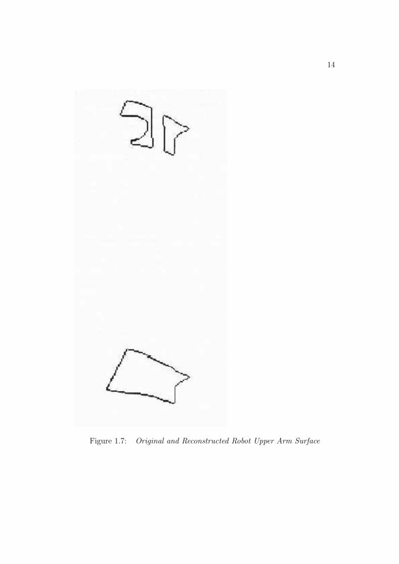
Image segmentation leads directly to partial or complete object surfacesegments. Surface completion processes (Chapter 4) reconstruct obscuredportions of surfaces, when possible, by connecting extrapolated surface bound-aries behind obscuring surfaces. The advantage of this is twofold: it providesdata surfaces more like the original object surface for property extractionand gives better image evidence during hypothesis construction. Two pro-cesses are used for completing surface hypotheses. The first bridges gaps insingle surfaces and the second links two separated surface patches. Mergedsurface segments must have roughly the same depth, orientation and surfacecharacterization. Because the reconstruction is based on three dimensionalsurface image data, it is more reliable than previous work that used only twodimensional image boundaries. Figure 1.7 illustrates both rules in showingthe original and reconstructed robot upper arm large surface from the test

12

Figure 1.4: Cosine of Surface Slant for the Test Scene

Figure 1.5: Obscuring Boundaries for the Test Scene

13

Figure 1.6: Shape Segmentation Boundaries for the Test Scene

image.

Surface Clusters

Surface hypotheses are joined to form surface clusters, which are blob-likethree dimensional object-centered representations (Chapter 5). The goal ofthis process is to partition the scene into a set of three dimensional solids,without yet knowing their identities. Surface clusters are useful (here) foraggregating image features into contexts for model invocation and matching.They would also be useful for tasks where identity is not necessary, such ascollision avoidance.

A surface cluster is formed by finding closed loops of isolating bound-ary segments. The goal of this process is to create a blob-like solid thatencompasses all and only the features associated with a single object. Thisstrengthens the evidence accumulation used in model invocation and limitscombinatorial matching during hypothesis construction. Obscuring and con-cave surface orientation discontinuity boundaries generally isolate solids, butan exception is for laminar objects, where the obscuring boundary across the

14

Figure 1.7: Original and Reconstructed Robot Upper Arm Surface

15

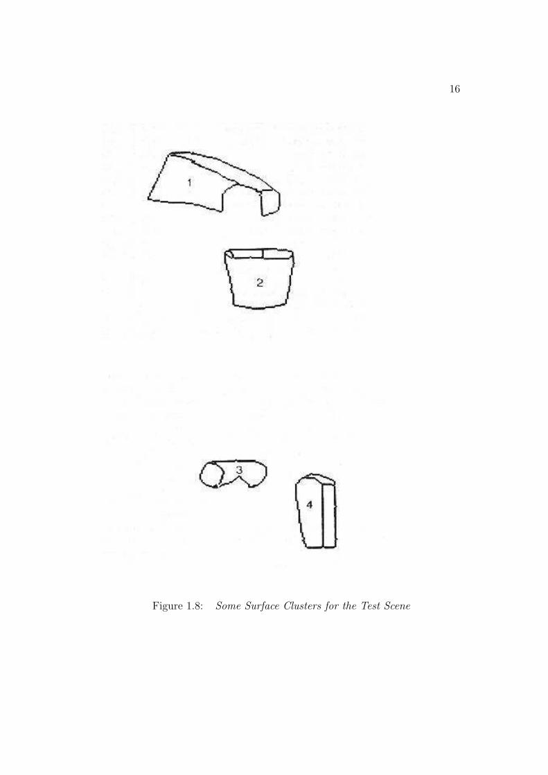
front lip of the trash can (Figure 1.8) does not isolate the surfaces. Thesecriteria determine the primitive surface clusters. A hierarchy of larger surfaceclusters are formed from equivalent depth and depth merged surface clusters,based on depth ordering relationships. They become larger contexts withinwhich partially self-obscured structure or subcomponents can be found. Fig-ure 1.8 shows some of the primitive surface clusters for the test scene. Theclusters correspond directly to primitive model ASSEMBLYs (which repre-sent complete object models).

Three Dimensional Feature Description

General identity-independent properties (Chapter 6) are used to drivethe invocation process to suggest object identities, which trigger the model-directed matching processes. Later, these properties are used to ensure thatmodel-to-data surface pairings are correct. The use of three dimensionalinformation from the surface image makes it possible to compute many objectproperties directly (as compared to computing them from a two dimensionalprojection of three dimensional data).

This task uses the surfaces and surface clusters produced by the segmen-tation processes. Surface and boundary shapes are the key properties forsurfaces. Relative feature sizes, spatial relationships and adjacency are theproperties needed for solid recognition. Most of the measured propertiesrelate to surface patches and include: local curvature, absolute area, elon-gation and surface intersection angles. As an example, Table 1.1 lists theestimated properties for the robot shoulder circular end panel (region 26 inFigure 3.10).

Surface-Based Object Representation

The modeled objects (Chapter 7) are compact, connected solids withdefinable shapes, where the complete surfaces are rigid and segmentable intoregions of constant local shape. The objects may also have subcomponentsjoined by interconnections with degrees-of-freedom.

Identification requires known object representations with three compo-nents: a geometric model, constraints on object properties, and a set ofinter-object relationships.

16

Figure 1.8: Some Surface Clusters for the Test Scene

17

Table 1.1: Properties of Robot Shoulder End Panel

PROPERTY ESTIMATED TRUE

maximum surface curvature 0.0 0.0

minimum surface curvature 0.0 0.0

absolute area 165 201

relative area 0.24 0.25

surface size eccentricity 1.4 1.0

adjacent surface angle 1.47 1.57

number of parallel boundaries 1 1

boundary curve length 22.5 25.1

boundary curve length 25.3 25.1

boundary curvature 0.145 0.125

boundary curvature 0.141 0.125

number of straight segments 0 0

number of arc segments 2 2

number of equal segments 1 1

number of right angles 0 0

boundary relative orientation 3.14 3.14

boundary relative orientation 3.14 3.14

18

The SURFACE patch is the model primitive, because surfaces are the pri-mary data units. This allows direct pairing of data with models, comparisonof surface shapes and estimation of model-to-data transformation parame-ters. SURFACEs are described by their principal curvatures with zero, oneor two curvature axes, and by their extent (i.e. boundary). The segmen-tation ensures that the shape (e.g. principal curvatures) remains relativelyconstant over the entire SURFACE.

Larger objects (called ASSEMBLYs) are recursively constructed fromSURFACEs or other ASSEMBLYs using coordinate reference frame transfor-mations. Each structure has its own local reference frame and larger struc-tures are constructed by placing the subcomponents in the reference frameof the aggregate. Partially constrained transformations can connect subcom-ponents by using variables in the attachment relationship. This was used forthe PUMA robot’s joints. The geometric relationship between structures isuseful for making model-to-data assignments and for providing the adjacencyand relative placement information used by verification.

The three major object models used in this analysis are the PUMA robot,chair and trash can. (These models required the definition of 25 SURFACEsand 14 ASSEMBLYs.) A portion of the robot model definition is shownbelow.

Illustrated first is the SURFACE definition for the robot upper arm largecurved end panel (uendb). The first triple on each line gives the startingendpoint for a boundary segment. The last item describes the segment as aLINE or a CURVE (with its parameters in brackets). PO means the segmen-tation point is a boundary orientation discontinuity point and BO means theboundary occurs at an orientation discontinuity between the surfaces. Thenext to last line describes the surface type with its axis of curvature and radii.The final line gives the surface normal at a nominal point in the SURFACE’sreference frame.

SURFACE uendb =

PO/(0,0,0) BO/LINE

PO/(10,0,0) BO/CURVE[0,0,-22.42]

PO/(10,29.8,0) BO/LINE

PO/(0,29.8,0) BO/CURVE[0,0,-22.42]

CYLINDER [(0,14.9,16.75),(10,14.9,16.75),22.42,22.42]

NORMAL AT (5,15,-5.67) = (0,0,-1);

19

Illustrated next is the rigid upperarm ASSEMBLY with its SURFACEs(e.g. uendb) and the reference frame relationships between them. The firsttriple in the relationship is the (x, y, z) translation and the second gives the(rotation, slant, tilt) rotation. Translation is applied after rotation.

ASSEMBLY upperarm\= =

uside AT ((-17,-14.9,-10),(0,0,0))

uside AT ((-17,14.9,0),(0,pi,pi/2))

uendb AT ((-17,-14.9,0),(0,pi/2,pi))

uends AT ((44.8,-7.5,-10),(0,pi/2,0))

uedges AT ((-17,-14.9,0),(0,pi/2,3*pi/2))

uedges AT ((-17,14.9,-10),(0,pi/2,pi/2))

uedgeb AT ((2.6,-14.9,0),(0.173,pi/2,3*pi/2))

uedgeb AT ((2.6,14.9,-10),(6.11,pi/2,pi/2));

The ASSEMBLY that pairs the upper and lower arm rigid structures intoa non-rigidly connected structure is defined now. Here, the lower arm has anaffixment parameter that defines the joint angle in the ASSEMBLY.

ASSEMBLY armasm =

upperarm AT ((0,0,0),(0,0,0))

lowerarm AT ((43.5,0,0),(0,0,0))

FLEX ((0,0,0),(jnt3,0,0));

Figure 1.9 shows an image of the whole robot ASSEMBLY with the sur-faces shaded according to surface orientation.

Property constraints are the basis for direct evidence in the model in-vocation process and for identity verification. These constraints give thetolerances on properties associated with the structures, and the importanceof the property in contributing towards invocation. Some of the constraintsassociated with the robot shoulder end panel named “robshldend” are givenbelow (slightly re-written from the model form for readability). The firstconstraint says that the relative area of the robshldend in the context of asurface cluster (i.e. the robot shoulder) should lie between 11% and 40%with a peak value of 25%, and the weighting of any evidence meeting thisconstraint is 0.5.

UNARYEVID 0.11\ < relative\_area < 0.40 PEAK 0.25 WEIGHT 0.5;

UNARYEVID 156.0 < absolute\_area < 248.0 PEAK 201.0 WEIGHT 0.5;

20

Figure 1.9: Shaded View of Robot Model

21

UNARYEVID 0.9 < elongation < 1.5 PEAK 1.0 WEIGHT 0.5;

UNARYEVID 0 < parallel\_boundary\_segments < 2 PEAK 1 WEIGHT 0.3;

UNARYEVID 20.1 < boundary\_length < 40.0 PEAK 25.1 WEIGHT 0.5;

UNARYEVID .08 < boundary\_curvature < .15 PEAK .125 WEIGHT 0.5;

BINARYEVID 3.04 < boundary\_relative\_orientation(edge1,edge2)

< 3.24 PEAK 3.14 WEIGHT 0.5;

Rather than specifying all of an object’s properties, it is possible to specifysome descriptive attributes, such as “flat”. This means that the so-describedobject is an instance of type “flat” – that is, “surfaces without curvature”.There is a hierarchy of such descriptions: the description “circle” given be-low is a specialization of “flat”. For robshldend, there are two descriptions:circular, and that it meets other surfaces at right angles:

DESCRIPTION OF robshldend IS circle 3.0;

DESCRIPTION OF robshldend IS sapiby2b 1.0;

Relationships between objects define a network used to accumulate in-vocation evidence. Between each pair of model structures, seven types ofrelationship may occur: subcomponent, supercomponent, subclass, super-class, descriptive, general association and inhibition. The model base definesthose that are significant to each model by listing the related models, thetype of relationship and the strength of association. The other relationshipfor robshldend is:

SUPERCOMPONENT OF robshldend IS robshldbd 0.10;

Evidence for subcomponents comes in visibility groups (i.e. subsets ofall object features), because typically only a few of an object’s features arevisible from any particular viewpoint. While they could be deduced compu-tationally (at great expense), the visibility groups are given explicitly here.The upperarm ASSEMBLY has two distinguished views, differing by whetherthe big (uendb) or small (uends) curved end section is seen.

SUBCGRP OF upperarm = uside uends uedgeb uedges;

SUBCGRP OF upperarm = uside uendb uedgeb uedges;

Model Invocation

22

Model invocation (Chapter 8) links the identity-independent processingto the model-directed processing by selecting candidate models for furtherconsideration. It is essential because of the impossibility of selecting thecorrect model by sequential direct comparison with all known objects. Thesemodels have to be selected through suggestion because: (a) exact individualmodels may not exist (object variation or generic description) and (b) objectflaws, sensor noise and data loss lead to inexact model-to-data matchings.

Model invocation is the purest embodiment of recognition – the inferenceof identity. Its outputs depend on its inputs, but need not be verified orverifiable for the visual system to report results. Because we are interestedin precise object recognition here, what follows after invocation is merelyverification of the proposed hypothesis: the finding of evidence and ensuringof consistency.

Invocation is based on plausibility, rather than certainty, and this notionis expressed through accumulating various types of evidence for objects inan associative network. When the plausibility of a structure having a givenidentity is high enough, a model is invoked.

Plausibility accumulates from property and relationship evidence, whichallows graceful degradation from erroneous data. Property evidence is ob-tained when data properties satisfy the model evidence constraints. Eachrelevant description contributes direct evidence in proportion to a weightfactor (emphasizing its importance) and the degree that the evidence fits theconstraints. When the data values from Table 1.1 are associated with theevidence constraints given above, the resulting property evidence plausibilityfor the robshldend panel is 0.57 in the range [-1,1].

Relationship evidence arises from conceptual associations with other struc-tures and identifications. In the test scene, the most important relationshipsare supercomponent and subcomponent, because of the structured nature ofthe objects. Generic descriptions are also used: robshldend is also a “circle”.Inhibitory evidence comes from competing identities. The modeled relation-ships for robshldend were given above. The evidence for the robshldendmodel was:

• property: 0.57

• supercomponent (robshould): 0.50

• description (circle, sapiby2b): 0.90

23

• inhibition: none

No inhibition was received because there were no competing identities withsufficiently high plausibility. All evidence types are combined (with weight-ing) to give an integrated evidence value, which was 0.76.

Plausibility is only associated with the model being considered and acontext; otherwise, models would be invoked for unlikely structures. In otherwords, invocation must localize its actions to some context inside which allrelevant data and structure must be found. The evidence for these structuresaccumulates within a context appropriate to the type of structure:

• individual model SURFACEs are invoked in a surface hypothesis con-text,

• SURFACEs associate to form an ASSEMBLY in a surface cluster con-text, and

• ASSEMBLYs associate in a surface cluster context.

The most plausible context for invoking the upper arm ASSEMBLY modelwas blob 1 in Figure 1.8, which is correct.

The invocation computation accumulates plausibility in a relational net-work of {context} × {identity} nodes linked to each other by relationshiparcs and linked to the data by the property constraints. The lower levelnodes in this network are general object structures, such as planes, positivecylinders or right angle surface junctions. From these, higher level objectstructures are linked hierarchically. In this way, plausibility accumulatesupwardly from simple to more complex structures. This structuring pro-vides both richness in discrimination through added detail, and efficiency ofassociation (i.e. a structure need link only to the most compact levels of sub-description). Though every model must ultimately be a candidate for everyimage structure, the network formulation achieves efficiency through judi-cious selection of appropriate conceptual units and computing plausibilityover the entire network in parallel.

When applied to the full test scene, invocation was generally successful.There were 21 SURFACE invocations of 475 possible, of which 10 were cor-rect, 5 were justified because of similarity and 6 were unjustified. There were18 ASSEMBLY invocations of 288 possible, of which 10 were correct, 3 werejustified because of similarity and 5 were unjustified.

24

Hypothesis Construction

Hypothesis construction (Chapter 9) aims for full object recognition, byfinding evidence for all model features. Invocation provides the model-to-data correspondences to form the initial hypothesis. Invocation thus elimi-nates most substructure search by directly pairing features. SURFACE cor-respondences are immediate because there is only one type of data element– the surface. Solid correspondences are also trivial because the matchedsubstructures (SURFACEs or previously recognized ASSEMBLYs) are alsotyped and are generally unique within the particular model. All other datamust come from within the local surface cluster context.

The estimation of the ASSEMBLY and SURFACE reference frames is onegoal of hypothesis construction. The position estimate can then be used formaking detailed metrical predictions during feature detection and occlusionanalysis (below).

Object orientation is estimated by transforming the nominal orientationsof pairs of model surface vectors to corresponding image surface vectors.Pairs are used because a single vector allows a remaining degree of rota-tional freedom. Surface normals and curvature axes are the two types ofsurface vectors used. Translation is estimated from matching oriented modelSURFACEs to image displacements and depth data. The spatial relation-ships between structures are constrained by the geometric relationships of themodel and inconsistent results imply an inappropriate invocation or featurepairing.

Because of data errors, the six degrees of spatial freedom are representedas parameter ranges. Each new model-to-data feature pairing contributesnew spatial information, which helps further constrain the parameter range.Previously recognized substructures also constrain object position.

The robot’s position and joint angle estimates were also found using ageometric reasoning network approach [74]. Based partly on the SUP/INFmethods used in ACRONYM [42], algebraic inequalities that defined therelationships between model and data feature positions were used to compilea value-passing network. The network calculated upper and lower boundson the (e.g.) position values by propagating calculated values through thenetwork. This resulted in tighter position and joint angle estimates thanachieved by the vector pairing approach.

25

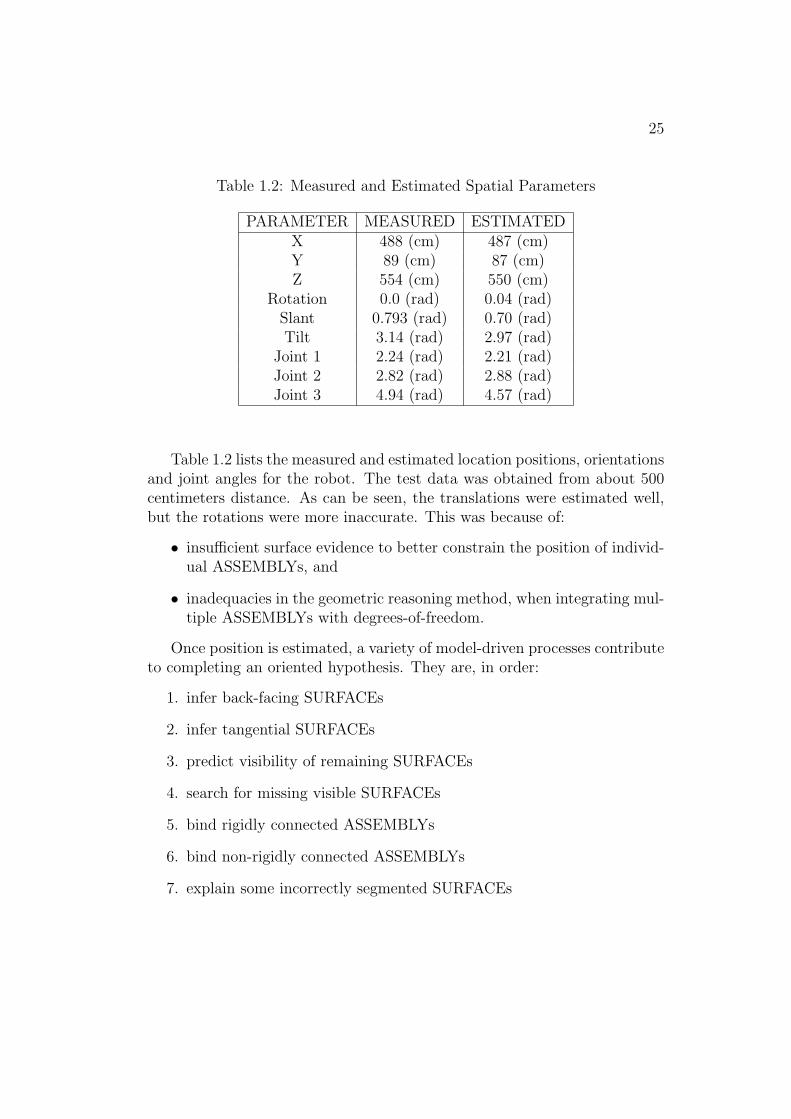
Table 1.2: Measured and Estimated Spatial Parameters

PARAMETER MEASURED ESTIMATEDX 488 (cm) 487 (cm)Y 89 (cm) 87 (cm)Z 554 (cm) 550 (cm)

Rotation 0.0 (rad) 0.04 (rad)Slant 0.793 (rad) 0.70 (rad)Tilt 3.14 (rad) 2.97 (rad)

Joint 1 2.24 (rad) 2.21 (rad)Joint 2 2.82 (rad) 2.88 (rad)Joint 3 4.94 (rad) 4.57 (rad)

Table 1.2 lists the measured and estimated location positions, orientationsand joint angles for the robot. The test data was obtained from about 500centimeters distance. As can be seen, the translations were estimated well,but the rotations were more inaccurate. This was because of:

• insufficient surface evidence to better constrain the position of individ-ual ASSEMBLYs, and

• inadequacies in the geometric reasoning method, when integrating mul-tiple ASSEMBLYs with degrees-of-freedom.

Once position is estimated, a variety of model-driven processes contributeto completing an oriented hypothesis. They are, in order:

1. infer back-facing SURFACEs

2. infer tangential SURFACEs

3. predict visibility of remaining SURFACEs

4. search for missing visible SURFACEs

5. bind rigidly connected ASSEMBLYs

6. bind non-rigidly connected ASSEMBLYs

7. explain some incorrectly segmented SURFACEs

26

Figure 1.10: Predicted Angle Between Robot Upper and Lower Arms

8. validate externally obscured structure

Hypothesis construction has a “hierarchical synthesis” character, wheredata surfaces are paired with model SURFACEs, surface groups are matchedto ASSEMBLYs and ASSEMBLYs are matched to larger ASSEMBLYs. Thethree key constraints on the matching are: localization in the correct im-age context (i.e. surface cluster), correct feature identities and consistentgeometric reference frame relationships.

Joining together two non-rigidly connected subassemblies also gives thevalues of the variable attachment parameters by unifying the respective ref-erence frame descriptions. The attachment parameters must also meet anyspecified constraints, such as limits on joint angles in the robot model. Forthe robot upper and lower arm, the joint angle jnt3 was estimated to be4.57, compared to the measured value of 4.94. Figure 1.10 shows the pre-dicted upper and lower arms at this angle.

27

Missing features, such as the back of the trash can, are found by a model-directed process. Given the oriented model, the image positions of unmatchedSURFACEs can be predicted. Then, any surfaces in the predicted area that:

• belong to the surface cluster,

• have not already been previously used and

• have the correct shape and orientation

can be used as evidence for the unpaired model features.Accounting for missing structure requires an understanding of the three

cases of feature visibility, predicting or verifying their occurrence and show-ing that the image data is consistent with the expected visible portion of themodel. The easiest case of back-facing and tangent SURFACEs can be pre-dicted using the orientation estimates with known observer viewpoint and thesurface normals deduced from the geometric model. A raycasting technique(i.e. predicting an image from an oriented model) handles self-obscured front-facing SURFACEs by predicting the location of obscuring SURFACEs andhence which portions of more distant SURFACEs are invisible. Self-occlusionis determined by comparing the number of obscured to non-obscured pixelsfor the front-facing SURFACEs in the synthetic image. This prediction alsoallows the program to verify the partially self-obscured SURFACEs, whichwere indicated in the data by back-side-obscuring boundaries. The final fea-ture visibility case occurs when unrelated structure obscures portions of theobject. Assuming enough evidence is present to invoke and orient the model,occlusion can be confirmed by finding closer unrelated surfaces responsiblefor the missing image data. Partially obscured (but not self-obscured) SUR-FACEs are also verified as being externally obscured. These SURFACEs arenoticed because they have back-side-obscuring boundaries that have not beenexplained by self-occlusion analysis.

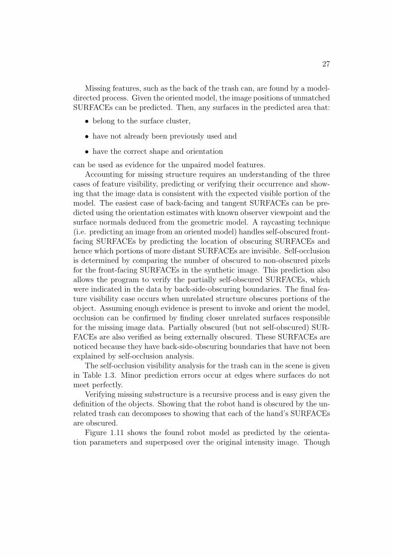
The self-occlusion visibility analysis for the trash can in the scene is givenin Table 1.3. Minor prediction errors occur at edges where surfaces do notmeet perfectly.

Verifying missing substructure is a recursive process and is easy given thedefinition of the objects. Showing that the robot hand is obscured by the un-related trash can decomposes to showing that each of the hand’s SURFACEsare obscured.

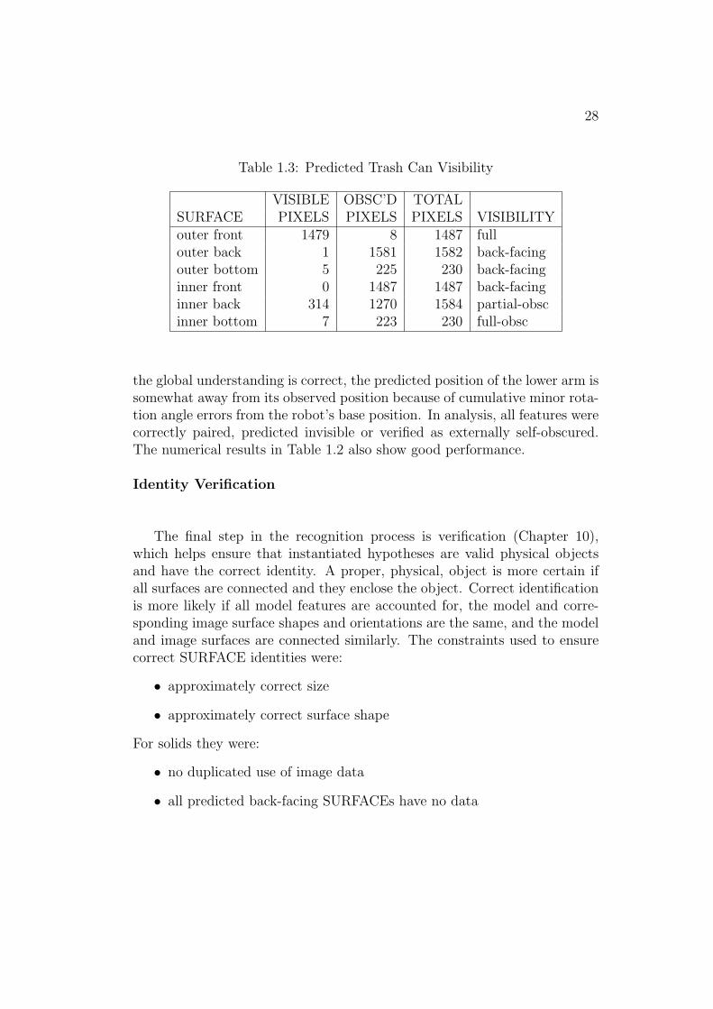
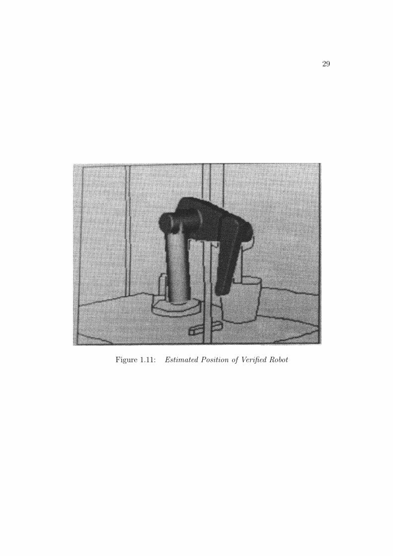
Figure 1.11 shows the found robot model as predicted by the orienta-tion parameters and superposed over the original intensity image. Though

28

Table 1.3: Predicted Trash Can Visibility

VISIBLE OBSC’D TOTALSURFACE PIXELS PIXELS PIXELS VISIBILITYouter front 1479 8 1487 fullouter back 1 1581 1582 back-facingouter bottom 5 225 230 back-facinginner front 0 1487 1487 back-facinginner back 314 1270 1584 partial-obscinner bottom 7 223 230 full-obsc

the global understanding is correct, the predicted position of the lower arm issomewhat away from its observed position because of cumulative minor rota-tion angle errors from the robot’s base position. In analysis, all features werecorrectly paired, predicted invisible or verified as externally self-obscured.The numerical results in Table 1.2 also show good performance.

Identity Verification

The final step in the recognition process is verification (Chapter 10),which helps ensure that instantiated hypotheses are valid physical objectsand have the correct identity. A proper, physical, object is more certain ifall surfaces are connected and they enclose the object. Correct identificationis more likely if all model features are accounted for, the model and corre-sponding image surface shapes and orientations are the same, and the modeland image surfaces are connected similarly. The constraints used to ensurecorrect SURFACE identities were:

• approximately correct size

• approximately correct surface shape

For solids they were:

• no duplicated use of image data

• all predicted back-facing SURFACEs have no data

29

Figure 1.11: Estimated Position of Verified Robot

30

• all adjacent visible model SURFACEs are adjacent in data

• all subfeatures have correct placement and identity

• all features predicted as partially self-obscured during raycasting areobserved as such (i.e. have appropriate obscuring boundaries)

In the example given above, all correct object hypotheses passed theseconstraints. The only spurious structures to pass verification were SUR-FACEs similar to the invoked model or symmetric subcomponents.

To finish the summary, some implementation details follow. The IMAG-INE I program was implemented mainly in the C programming languagewith some PROLOG for the geometric reasoning and invocation networkcompilation (about 20,000 lines of code in total). Execution required about8 megabytes total, but this included several 256*256 arrays and generousstatic data structure allocations. Start-to-finish execution without graphicson a SUN 3/260 took about six minutes, with about 45% for self-occlusionanalysis, 20% for geometric reasoning and 15% for model invocation. Many ofthe ideas described here are now being used and improved in the IMAGINEII program, which is under development.

The completely recognized robot is significantly more complicated thanpreviously recognized objects (because of its multiple articulated features,curved surfaces, self-occlusion and external occlusion). This successful com-plete, explainable, object recognition was achieved because of the rich infor-mation embedded in the surface data and surface-based models.

Recognition Graph Summary

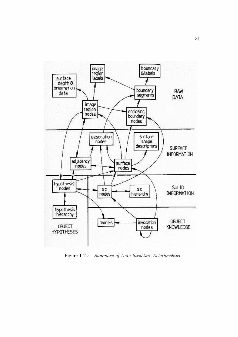
The recognition process creates many data structures, linked into a graphwhose relationships are summarized in Figure 1.12. This figure should bereferred to while reading the remainder of this book.

At the top of the diagram, the three bubbles “surface depth and orienta-tion data”, “image region labels” and “boundary and labels” are the imagedata input. The boundary points are linked into “boundary segments” whichhave the same label along their entire length. “Image region nodes” representthe individual surface image regions with their “enclosing boundary nodes”,which are circularly linked boundary segments. “Adjacency nodes” link ad-

31

Figure 1.12: Summary of Data Structure Relationships

32

jacent region nodes and also link to “description nodes” that record whichboundary separates the regions.

The “image region nodes” form the raw input into the “surface nodes”hypothesizing process. The “surface nodes” are also linked by “adjacencynodes” and “enclosing boundary nodes”. In the description phase, proper-ties of the surfaces are calculated and these are also recorded in “descriptionnodes”. Surface shape is estimated and recorded in the “surface shape de-scriptors”.

The surface cluster formation process aggregates the surfaces into groupsrecorded in the “surface cluster nodes”. These nodes are organized into a“surface cluster hierarchy” linking larger enclosing or smaller enclosed surfaceclusters. The surface clusters also have properties recorded in “descriptionnodes” and have an enclosing boundary.

Invocation occurs in a plausibility network of “invocation nodes” linkedby the structural relations given by the “models”. Nodes exist linking modelidentities to image structures (surface or surface cluster nodes). The invoca-tion nodes link to each other to exchange plausibility among hypotheses.

When a model is invoked, a “hypothesis node” is created linking the modelto its supporting evidence (surface and surface cluster nodes). Hypothesesrepresenting objects are arranged in a component hierarchy analogous to thatof the models. Image region nodes link to the hypotheses that best explainthem.

This completes our overview of the recognition process and the followingchapters explore the issues raised here in depth.

Chapter 2

Object Recognition fromSurface Information

Intuitively, object recognition is the isolation and identification of structurefrom the midst of other detail in an image of a scene. It is also the assignmentof a symbol to a group of features with the implication that those featurescould only belong to an object designated by that symbol. Hence, when wesay we perceive (recognize) “John”, we assert that there is a person named“John”, who accounts for all the perceived features, and that this person isat the specified location in the given scene.

When described like this, object recognition seems little different froma general concept-matching paradigm. So, what distinguishes it as a visionproblem? The answer lies in the types of data, its acquisition, the viewer-to-object geometry, the image projection relationship and the representations ofstructures to be recognized. This research addresses several aspects of howto perceive structure [166] visually:

• What are some of the relevant structures in the data?

• How is their appearance transformed by the visual process?

• How are they represented as a set of models?

• How are the models selected?

• How is the model-to-data correspondence established?

33

34

Visual recognition involves reasoning processes that transform betweeninternal representations of the scene, linking the lower levels of image descrip-tion to the higher levels of object description. The transformations reflectboth the relationships between the representations and the constraints onthe process. The most important constraints are those based on the physicalproperties of the visual domain and the consequent relationships betweendata elements.

Vision does have aspects in common with other cognitive processes –notably model invocation and generalization. Invocation selects candidatemodels to explain sets of data, a task that, in function, is no different fromselecting “apple” as a unifying concept behind the phrase “devilish fruit”.Invocation makes the inductive leap from data to explanation, but only ina suggestive sense, by computing from associations among symbolic descrip-tions. Generalization also plays a big role in both recognition and otherprocesses, because one needs to extract the key features, and gloss over theirrelevant ones, to categorize a situation or object.

The first half of this chapter considers the problem of recognition in gen-eral, and the second half discusses previous approaches to recognition.

2.1 The Nature of Recognition

Visual recognition (and visual perception) has received considerable philo-sophical investigation. Three key results are mentioned, as an introductionto this section.

(1) Perception interprets raw sensory data. For example, we interpret aparticular set of photons hitting our retina as “green”. As a result, perceptionis an internal phenomenon caused by external events. It transforms thesensory phenomena into a reference to a symbolic description. Hence, there isa strong “linguistic” element to recognition – a vocabulary of interpretations.The perception may be directly related to the source, but it may also be amisinterpretation, as with optical illusions.

(2) Interpretations are directly dependent on the theories about whatis being perceived. Hence, a theory that treats all intensity discontinuitiesas instances of surface reflectance discontinuities will interpret shadows asunexplained or reflectance discontinuity phenomena.

(3) Identity is based on conceptual relations, rather than purely physicalones. An office chair with all atoms replaced by equivalent atoms or one

35

that has a bent leg is still a chair. Hence, any object with the appropriateproperties could receive the corresponding identification.

So, philosophical theory implies that recognition has many weaknesses:the interpretations may be fallacious, not absolute and reductive. In practice,however, humans can effectively interpret unnatural or task-specific scenes(e.g. x-ray interpretation for tuberculosis detection) as well as natural andgeneral ones (e.g. a tree against the sky). Moreover, almost all humans arecapable of visually analyzing the world and producing largely similar descrip-tions of it. Hence, there must be many physical and conceptual constraintsthat restrict interpretation of both raw data as image features, and the re-lation of these features to objects. This chapter investigates the role of thesecond category on visual interpretation.

How is recognition understood here? Briefly, recognition is the productionof symbolic descriptions. A description is an abstraction, as is stored objectknowledge. The production process transforms sets of symbols to produceother symbols. The transformations are guided (in practice) by physical,computational and efficiency constraints, as well as by observer history andby perceptual goals.

Transformations are implementation dependent, and may be erroneous,as when using a simplified version of the ideal transformation. They can alsomake catastrophic errors when presented with unexpected inputs or whenaffected by distorting influences (e.g. optical, electrical or chemical). Thenotion of “transformation error” is not well founded, as the emphasis here isnot on objective reality but on perceptual reality, and the perceptions nowexist, “erroneous” or otherwise. The perceptions may be causally initiated bya physical world, but they may also be internally generated: mental imagery,dreams, illusions or “hallucinations”. These are all legitimate perceptionsthat can be acted on by subsequent transformations; they are merely not“normal” or “well-grounded” interpretations.

Normal visual understanding is mediated by different description typesover a sequence of transformations. The initial representation of a symbolmay be by a set of photons; later channels may be explicit (value, place orsymbol encoded), implicit (connectionist) or external. The communicationof symbols between processes (or back into the same process) is also subjectto distorting transformations.

In part, identity is linguistic: a chair is whatever is called a chair. It is alsofunctional – an object has an identity only by virtue of its role in the humanworld. Finally, identity implies that it has properties, whether physical or

36

mental. Given that objects have spatial extension, and are complex, someof the most important properties are linked to object substructures, theiridentity and their placement.

An identification is the attribution of a symbol whose associated proper-ties are similar to those of the data, and is the output of a transformation.The properties (also symbols) compared may come from several different pro-cesses at different stages of transformation. Similarity is not a well definednotion, and seems to relate to a conceptual distance relationship in the spaceof all described objects. The similarity evaluation is affected by perceptualgoals.

This is an abstract view of recognition. The practical matters are nowdiscussed: what decisions must be made for an object recognition system tofunction in practice.

Descriptions and Transformations

This research starts at the 212D sketch, so this will be the first description

encountered. Later transformations infer complete surfaces, surface clusters,object properties and relationships and object hypotheses, as summarized inChapter 1.

As outlined above, each transformation is capable of error, such as in-correctly merging two surfaces behind an obscuring object, or hypothesizinga non-existent object. Moreover, the model invocation process is designedto allow “errors” to occur, as such a capability is needed for generic objectrecognition, wherein only “close” models exist. Fortunately, there are manyconstraints that help prevent the propagation of errors.

Some symbols are created directly from the raw data (e.g. surface prop-erties), but most are created by transforming previously generated results(e.g. using two surfaces as evidence for hypothesizing an object containingboth).

Object Isolation

Traditionally, recognition involves structure isolation, as well as identifi-cation, because naming requires objects to be named. This includes denotingwhat constitutes the object, where it is and what properties it has. Unfor-

37

tunately, the isolation process depends on what is to be identified, in thatwhat is relevant can be object-specific. However, this problem is mitigatedbecause the number of general visual properties seems to be limited and thereis hope of developing “first pass” grouping techniques that could be largelyautonomous and model independent. (These may not always be model inde-pendent, as, for example, the constellation Orion can be found and declaredas distinguished in an otherwise random and overlapping star field.) So, partof a sound theory of recognition depends on developing methods for isolatingspecific classes of objects. This research inferred surface groupings from localintersurface relationships.

The Basis for Recognition

Having the correct properties and relationships is the traditional basis forrecognition, with the differences between approaches lying in the types of evi-dence used, the modeling of objects, the assumptions about what constitutesadequate recognition and the algorithms for performing the recognition.

Here, surface and structure properties are the key types of evidence, andthey were chosen to characterize a large class of everyday objects. As threedimensional input data is used, a full three dimensional description of theobject can be constructed and directly compared with the object model. Allmodel feature properties and relationships should be held by the observeddata features, with geometric consistency as the strongest constraint. Thedifficulty then arises in the construction of the three dimensional description.Fortunately, various constraints exist to help solve this problem.

This research investigates recognizing “human scale” rigidly and non-rigidly connected solids with uniform, large surfaces including: classroomchairs, most of a PUMA robot and a trash can. The types of scenes in whichthese objects appear are normal indoor somewhat cluttered work areas, withobjects at various depths obscuring portions of other objects.

Given these objects and scenes, four groups of physical constraints areneeded:

• limitations on the surfaces and how they can be segmented and char-acterized,

• properties of solid objects, including how the surfaces relate to theobjects bounded by them,

38

• properties of scenes, including spatial occupancy and placement of ob-jects and

• properties of image formation and how the surfaces, objects and scenesaffect the perceived view.

Definition of Recognition

Recognition produces a largely instantiated, spatially located, describedobject hypothesis with direct correspondences to an isolated set of imagedata. “Largely instantiated” means that most object features predicted bythe model have been accounted for, either with directly corresponding imagedata or with explanations for their absence.

What distinguishes recognition, in the sense used in this book, is that itlabels the data, and hence is able to reconstruct the image. While the objectdescription may be compressed (e.g. a “head”), there will be an associatedprototypical geometric model (organizing the properties) that could be usedto recreate the image to the level of the description. This requires thatidentification be based on model-to-data correspondences, rather than onsummary quantities such as volume or mass distribution.

One problem with three dimensional scenes is incomplete data. In partic-ular, objects can be partially obscured. But, because of redundant features,context and limited environments, identification is still often possible. Onthe other hand, there are also objects that cannot be distinguished without amore complete examination – such as an opened versus unopened soft drinkcan. If complete identification requires all properties to be represented in thedata, any missing ones will need to be justified. Here, it is assumed that allobjects have geometric models that allow appearance prediction. Then, ifthe prediction process is reasonable and understands physical explanationsfor missing data (e.g. occlusion, known defects), the model will be consistentwith the observed data, and hence be an acceptable identification.

Criteria for Identification

The proposed criterion is that the object has all the right properties andnone of the wrong ones, as specified in the object model. The properties will

39

include local and global descriptions (e.g. surface curvatures and areas), sub-component existence, global geometric consistency and visibility consistency(i.e. what is seen is what is expected).

Perceptual goals determine the properties used in identification. Unusedinformation may allow distinct objects to acquire the same identity. If thegeneric chair were the only chair modeled, then all chairs would be classifiedas the generic chair.

The space of all objects does not seem to be sufficiently disjoint so thatthe detection of only a few properties will uniquely characterize them. Insome model bases, efficient recognition may be possible by a parsimoniousselection of properties, but redundancy adds the certainty needed to copewith missing or erroneous data, as much as the extra data bits in an errorcorrecting code help disperse the code space.

Conversely, a set of data might implicate several objects related througha relevant common generalization, such as (e.g.) similar yellow cars. Or,there may be no physical generalization between alternative interpretations(e.g., as in the children’s joke Q:“What is grey, has four legs and a trunk?”A:“A mouse going on a holiday!”).

Though the basic data may admit several interpretations, further associ-ated properties may provide finer identifications, much as ACRONYM [42]used additional constraints for class specialization.

While not all properties will be needed for a particular identification,some will be essential and recognition should require these when identifyingan object. One could interpret a picture of a soft drink can as if it were theoriginal, but this is just a matter of choosing what properties are relevant.An observation that is missing some features, such as one without the labelon the can, may suggest the object, but would not be acceptable as a properinstance.

There may also be properties that the object should not have, thoughthis is a more obscure case. In part, these properties may contradict theobject’s function. Some care has to be applied here, because there are manyproperties that an object does not have and all should not have to be madeexplicit. No “disallowed” properties were used here.

Most direct negative properties, like “the length cannot be less than 15cm” can be rephrased as “the length must be at least 15 cm”. Propertieswithout natural complements are less common, but exist: “adjacent to” and“subcomponent of” are two such properties. One might discriminate betweentwo types of objects by stating that one has a particular subcomponent,

40

and that the other does not and is otherwise identical. Failure to includethe “not subcomponent of” condition would reduce the negative case to ageneralization of the positive case, rather than an alternative. Examples ofthis are: a nail polish dot that distinguishes “his and her” toothbrushes or aback support as the discriminator between a chair and a stool.

Recognition takes place in a context – each perceptual system will haveits own set of properties suitable for discriminating among its range of ob-jects. In the toothbrushes example, the absence of the mark distinguishedone toothbrush in the home, but would not have been appropriate whenstill at the factory (among the other identical, unmarked, toothbrushes).The number and sensitivity of the properties affects the degree to whichobjects are distinguished. For example, the area-to-perimeter ratio distin-guishes some objects in a two dimensional vision context, even though it isan impoverished representation. This work did not explicitly consider anycontext-specific identification criteria.

The above discussion introduces most of the issues behind recognition,and is summarized here:

• the goals of recognition influence the distinguishable objects of thedomain,

• the characterization of the domain may be rich enough to provideunique identifications even when some data is missing or erroneous,

• all appropriate properties should be necessary, with some observed andthe rest deduced,

• some properties may be prohibited and

• multiple identifications may occur for the same object and additionalproperties may specialize them.

2.2 Some Previous Object Recognition Sys-

tems

Three dimensional object recognition is still largely limited to blocks worldscenes. Only simple, largely polyhedral objects can be fully identified, whilemore complicated objects can only be tentatively recognized (i.e. evidence

41

for only a few features can be found). There are several pieces of researchthat deserve special mention.

Roberts [139] was the founder of three dimensional model-based sceneunderstanding. Using edge detection methods, he analyzed intensity imagesof blocks world scenes containing rectangular solids, wedges and prisms. Thetwo key descriptions of a scene were the locations of vertices in its edge de-scription and the configurations of the polygonal faces about the vertices.The local polygon topology indexed into the model base, and promoted ini-tial model-to-data point correspondences. Using these correspondences, thegeometric relationship between the model, scene and image was computed.A least-squared error solution accounted for numerical errors. Object scaleand distance were resolved by assuming the object rested on a ground planeor on other objects. Recognition of one part of a configuration introducednew edges to help segment and recognize the rest of the configuration.

Hanson and Riseman’s VISIONS system [83] was proposed as a completevision system. It was a schema-driven natural scene recognition system act-ing on edge and multi-spectral region data [82]. It used a blackboard systemwith levels for: vertices, segments, regions, surfaces, volumes, objects andschemata. Various knowledge sources made top-down or bottom-up addi-tions to the blackboard. For the identification of objects (road, tree, sky,grass, etc.) a confidence value was used, based on property matching. Theproperties included: spectral composition, texture, size and two dimensionalshape. Rough geometric scene analysis estimated the base plane and thenobject distances knowing rough object sizes. Use of image relations to giverough relative scene ordering was proposed. Besides the properties, schematawere the other major object knowledge source. They organized objects likelyto be found together in generic scenes (e.g. a house scene) and providedconditional statistics used to direct the selection of new hypotheses from theblackboard to pursue.

As this system was described early in its development, a full evaluationcan not be made here. Its control structure was general and powerful, but itsobject representations were weak and dependent mainly on a few discriminat-ing properties, with little spatial understanding of three dimensional scenes.

Marr [112] hypothesized that humans use a volumetric model-based ob-ject recognition scheme that:

• took edge data from a 212D sketch,

• isolated object regions by identifying obscuring contours,

42

• described subelements by their elongation axes, and objects by the localconfiguration of axes,

• used the configurations to index into and search in a subtype/subcomponentnetwork representing the objects, and

• used image axis positions and model constraints for geometric analysis.

His proposal was outstanding in the potential scope of recognizable ob-jects, in defining and extracting object independent descriptions directlymatchable to three dimensional models (i.e. elongation axes), in the sub-type and subcomponent model refinement, and in the potential of its invo-cation process. It suffered from the absence of a testable implementation,from being too serial in its view of recognition, from being limited to onlycylinder-like primitives, from not accounting for surface structure and fromnot fully using the three dimensional data in the 21

2D sketch.

Brooks [42], in ACRONYM, implemented a generalized cylinder basedrecognizer using similar notions. His object representation had both sub-type and subcomponent relationships. From its models, ACRONYM derivedvisible features and relationships, which were then graph-matched to edgedata represented as ribbons (parallel edge groups). ACRONYM deducedobject position and model parameters by back constraints in the predictiongraph, where constraints were represented by algebraic inequalities. Thesesymbolically linked the model and position parameters to the model relation-ships and image geometry, and could be added to incrementally as recogni-tion proceeded. The algebraic position-constraint and incremental evidencemechanism was powerful, but the integration of the constraints was a time-consuming and imperfect calculation.

This well developed project demonstrated the utility of explicit geometricand constraint reasoning, and introduced a computational model for genericidentification based on nested sets of constraints. Its weakness were that itonly used edge data as input, it had a relatively incomplete understanding ofthe scene, and did not really demonstrate three dimensional understanding(the main example was an airplane viewed from a great perpendicular height).

Faugeras and his group [63] researched three dimensional object recog-nition using direct surface data acquired by a laser triangulation process.Their main example was an irregular automobile part. The depth valueswere segmented into planar patches using region growing and Hough trans-form techniques. These data patches were then combinatorially matched to

43

model patches, constrained by needing a consistent model-to-data geometrictransformation at each match. The transformation was calculated using sev-eral error minimization methods, and consistency was checked first by a fastheuristic check and then by error estimates from the transformation estima-tion. Their recognition models were directly derived from previous views ofthe object and record the parameters of the planar surface patches for theobject from all views.

Key problems here were the undirected matching, the use of planar patchesonly, and the relatively incomplete nature of their recognition – pairing ofa few patches was enough to claim recognition. However, they succeeded inthe recognition of a complicated real object.

Bolles et al. [36] used light stripe and laser range finder data. Surfaceboundaries were found by linking corresponding discontinuities in groups ofstripes, and by detecting depth discontinuities in the range data. Matchingto models was done by using edge and surface data to predict circular andhence cylindrical features, which were then related to the models. The keylimitation of these experiments was that only large (usually planar) surfacescould be detected, and so object recognition could depend on only thesefeatures. This was adequate in the limited industrial domains. The mainadvantages of the surface data was that it was absolute and unambiguous,and that planar (etc.) model features could be matched directly to otherplanar (etc.) data features, thus saving on matching combinatorics.

The TINA vision system, built by the Sheffield University Artificial Intel-ligence Vision Research Unit [134], was a working stereo-based three dimen-sional object recognition and location system. Scene data was acquired inthree stages: (1) subpixel “Canny” detected edges were found for a binocularstereo image pair, (2) these were combined using epipolar, contrast gradientand disparity gradient constraints and (3) the three dimensional edge pointswere grouped to form straight lines and circular arcs. These three dimen-sional features were then matched to a three dimensional wire frame model,using a local feature-focus technique [35] to cue the initial matches. Theyeliminated the incorrect model-to-data correspondences using pairwise con-straints similar to those of Grimson and Lozano-Perez [78] (e.g. relativeorientation). When a maximal matching was obtained, a reference framewas estimated, and then improved by exploiting object geometry constraints(e.g. that certain lines must be parallel or perpendicular).

A particularly notable achievement of this project was their successfulinference of the wire frame models from multiple known views of the object.

44

Although the stereo and wire frame-based techniques were suited mainly forpolyhedral objects, this well-engineered system was successful at buildingmodels that could then be used for object recognition and robot manipula-tion.

More recently, Fan et al. [61] described range-data based object recogni-tion with many similarities to the work in this book. Their work initiallysegments the range data into surface patches at depth and orientation dis-continuities. Then, they created an attributed graph with nodes representingsurface patches (labeled by properties like area, orientation and curvature)and arcs representing adjacency (labeled by the type of discontinuity andestimated likelihood that the two surfaces are part of the same object). Thewhole scene graph is partitioned into likely complete objects (similar to oursurface clusters) using the arc likelihoods. Object models were representedby multiple graphs for the object as seen in topologically distinct viewpoints.The first step of model matching was a heuristic-based preselection of likelymodel graphs. Then, a search tree was formed, pairing compatible modeland data nodes. When a maximal set was obtained, and object position wasestimated , which was used to add or reject pairings. Consistent pairingsthen guided re-partitioning of the scene graph, subject to topological andgeometric consistency.

Rosenfeld [142] proposed an approach to fast recognition of unexpected(i.e. fully data driven) generic objects, based on five assumptions:

1. objects were represented in characteristic views,

2. the key model parts are regions and boundaries,

3. features are characterized by local properties,

4. relational properties are expressed in relative form (i.e. “greater then”)and

5. all properties are unidimensional and unimodal.

A consequence of these assumptions is that most of the recognition processesare local and distributed, and hence can be implemented on an (e.g.) pyra-midal processor.

This concludes a brief discussion of some prominent three dimensionalobject recognition systems. Other relevant research is discussed where ap-propriate in the main body of the book. Besl and Jain [23] gave a thorough

45

review of techniques for both three dimensional object representation andrecognition.

2.3 Recognition Approaches

This section summarizes the four traditional approaches to object recogni-tion, roughly in order of discriminating power. Most recognition systems useseveral techniques.

Property Based Identification

When enough model properties are satisfied by the data, recognition oc-curs. The properties may be scene location, orientation, size, color, shapeor others. The goal is unique discrimination in the model base, so judiciouschoice of properties is necessary. Duda and Hart’s [55] analysis of an officescene typified this. Other examples include Brice and Fennema [41], whoclassified regions by their boundary shape and defined object identity by agroup of regions with the correct shapes, and Adler [3], who ranked matchesby success at finding components meeting structural relationships and sum-mary properties. Property comparison is simple and efficient, but is notgenerally powerful enough for a large model base or subtle discriminations.The problem is always – “which properties?”.

Property matchers often use pattern recognition based discriminationmethods, implemented as sequential property comparison, decision trees ordistance based classifiers. These are straightforward, but do not easily allowcomplicated recognition criteria (e.g. geometric or relational) without priorcalculation of all potential properties, and treat objects at a single level ofrepresentation.

Given that properties are often continuous valued, and subject to error,a distance metric is often used to evaluate the match (e.g. [161]). If theproperties fit a statistical distribution, then a probabilistic classifier can beused (e.g. [56]).

Grammatical and Graph Matching

46

Here, recognition is achieved when a particular grouping of data is struc-turally identical to a similar model pattern. This usually expresses relation-ships between image features, such as edges or regions, but may also refer torelationships in three dimensional data. This method requires evaluation ofthe match between individual features.

For objects with primitive distinguishable features that have fixed rela-tionships (geometric or topological), two general methods have been devel-oped. The first is the syntactic method (e.g. [115, 46]). Valid relationshipsare embodied in grammar rules and recognition is done by parsing the datasymbols according to these rules. Rosenfeld [140] presented a typical exampleof this matching method by using web grammars for analyzing two dimen-sional patterns. The main applications of grammatical techniques have beenin fingerprint [117], circuit diagram, chromosome and texture analysis. Avariation on this method uses rules to recognize specific features (e.g. vege-tation in an aerial image [119] or urban building scenes [123]).

The second general matching technique is graph matching, where thegoal is to find a pairing between subsets of the data and model graphs.Two key techniques are subgraph isomorphism and maximal clique findingin association graphs [18]. Barrow and Popplestone [16] used a subgraphmatching between their data and model graphs. Ambler et al. [8] recognizedby using a maximal clique method in an association graph between data andmodels. Combinatorial explosion can be controlled by using a hierarchy ofstructures [17] and Turner [161] exploited this method procedurally in hishierarchical synthesis matcher.

One advantage of graph matching is that it is well understood and pro-duces understandable results through symbol matching, formal definitionand computationally analyzable machinery. Unfortunately, graph methodstend to be NP-complete and are not practical unless the graph size is small.Matching would be more efficient if geometric predictions were used, allow-ing direct comparison instead of the complete matching that general graphmatching algorithms require. Another disadvantage is that three dimen-sional scenes have changing viewpoints and occlusion, which distorts andfragments object descriptions (unless multiple graphs are used for alterna-tive viewpoints).

Heuristic match criteria are still needed for comparing nodes and arcs, andfor ranking subgraph matches. Barrow and Popplestone [16] used a heuristicweighting to evaluate the satisfaction of a subgraph match, including a factorthat favored larger matches. Ambler et al. [8] used similarity of properties

47

and relations between regions in a two dimensional parts scene. Nevatia andBinford [121] evaluated matches based on components found and parametercomparisons for the primitives.

Geometric Matching

Here, the geometric relationships in the model, initial object locationknowledge and image feature geometry combine to allow direct matching.Roberts [139], Freuder [75], Marr [112] and others argued that partial match-ing of image data to object models could be used to constrain where otherfeatures were and how to classify them. Locating this data then further con-strained the object’s geometric location as well as increasingly confirmed itsidentity.

Adler [3] used a top-down control regime to predict image location in twodimensional scenes, and explained data lost because of occlusion. Freuder [75]described a two dimensional recognition program that used active reasoningto recognize a hammer in image region data. The program used image modelsto obtain suggestions about what features to look for next and advice onwhere to find the features.

Matching may be almost totally a matter of satisfying geometric criteria.The advantage of geometric matching is that the matching criteria are usuallyclear and geometric models allow directed comparisons. One might requirethat the accumulated error between predicted and observed features be belowa threshold. For example, Faugeras and Hebert [63] used the model-to-data surface pairings that passed a geometric consistency measure and hadminimum transformation estimation error.

Roberts [139] estimated the transformation from selected model pointsto image points. Transformation errors exceeding a threshold implied a badmatch. Ikeuchi [96] recognized and oriented objects by computationally ro-tating extended gaussian images until good correspondences were achieved.Hogg [91] improved positional estimates using search over a bounded pa-rameter space. The estimates were used to predict the position of edgepoints, and the number of verified edge points was used evaluate the esti-mates. Ballard and Tanaka [15] used a connectionist method for deducing apolyhedral object’s reference frame given network linkages specified by geo-metric constraints. This follows Ballard’s work [12] on extracting componentparameters from intrinsic images by using Hough transform techniques.

48

Correct geometry is a strong constraint on an object’s identity. Its lim-itations include the need for pairing the appropriate structures, control ofcombinatorial matching and integration with other matchables, such as struc-tural properties and relationships.

Constraint Satisfaction

Implicit in the above methods are certain constraints that the data mustsatisfy. These constraints may apply to individual features, or to groups offeatures, or to relationships between features. Some researchers have triedto generalize the constraints by making them explicit. Matching algorithmscan use direct search, graph matching (where the constraints specify the nodeand arc match criteria) or relaxation. Relaxation algorithms can apply todiscrete symbol labelings [162], probabilistic labelings ([172, 141, 22, 62]) ora combination of the two [19]. Barrow and Tenenbaum [19] used adjacencyand homogeneity constraints to deduce identity in office scenes using height,intensity and orientation data. Hinton [86] formulated the substructure iden-tity problem as a relaxation problem, with the goal of maximizing credibilitysubject to model constraints.

Nevatia and Binford [121] matched models using connectivity relation-ships between generalized cylinder primitives in the model and data to con-strain correspondences. In ACRONYM [42], an object was identified bymaximal refinement in a specialization lattice consistent with both the modelconstraints and image data. The refinement was by constraint satisfaction,where the constraints mainly applied to feature sizes and relationships. Con-straint satisfaction was checked by inequality testing.

The constraint satisfaction approach encompasses the other methods de-scribed above. The ability of a constraint to be general is a real advantage,particularly when representing ranges of numerical values. Its weakness is itrequires the choice of constraints that efficiently and adequately discriminatewithout rejection of minor undistinguished variants.

Most systems use a combination of the methods to recognize objects inmore sophisticated scenes. For example, ACRONYM’s [42] matching algo-rithm looked for subgraph isomorphisms between the picture graph, repre-senting located image features, and the prediction graph, which was a pre-compilation of the object models. This graph tried to represent the likelysizes and intercomponent relationships between primitives, as seen in typical

49

views of the object. A node or arc match required not only local, but alsoglobal satisfaction of constraints such as requiring all features to have thesame reference frame.

The goal of most algorithms (but not ACRONYM’s) was to use local con-straints to produce global consistency. The difficulty with these pure meth-ods is that they excessively simplify and ignore most of the global structuralrelationships between nameable object features.

Matching algorithms generally follow a combinatorial tree-search approach,where each new level in the tree pairs a new data feature to a model feature.Full tree expansion is usually prevented by using constraints to remove badexpansions (e.g. those coming from predictions of positions). For example,Faugeras and Hebert [63] and Grimson and Lozano-Perez [78] successfullyused local relative position constraints to prune the search tree dramatically.

An improvement on the above basic methods is hierarchical recognition,in which objects are structured into levels of representation, and recognitionmatches components at the same level. Turner [161], Ambler et al. [8] andFisher [66] used a bottom-up “hierarchical synthesis” process [145] and Adler[3] used top-down model directed analysis.

Final Comments

This completes a quick review of the philosophical and historical back-ground to the research, and we now proceed to look at the research itself.

Chapter 3

Surface Data as Input forRecognition

Choosing surface data as the foundation for a theory of object recognition isnot without controversy, particularly given its unsuitability for all domainsand applications. None the less, it is justified in scenes where knowledgeof the three dimensional scene structure is important, as discussed in thischapter.

3.1 The Labeled Segmented Surface Image

The labeled segmented surface image is the primary data input for the recog-nition processes described in this book. Each of these terms is discussed ingreater detail below, but, by way of introduction, a surface image is a densepointillistic two-dimensional image representation, whose geometry arisesfrom a projective transformation of the three dimensional scene, and whosecontent describes properties of the visible surfaces in the scene. Segmentationpartitions the surface into regions of uniform properties (namely curvatureand continuity) and identifies the type of boundary between surface regions(e.g. whether obscuring or shape).

Surface Images

Surface images are an iconic representation similar in structure to tra-

50

51

ditional intensity images, except that they record surface properties, suchas absolute depth and surface orientation in the camera coordinate system.The positional relationship between the scene and the image is described byprojective geometry. In this way, surface images are a subset of intrinsicimages [20], except that here the information is solely related to the surfaceshape, and not to reflectance. This eliminates surface markings, shadows,highlights, image flow, shading and other illumination and observer depen-dent effects from the information (which are also important, but are notconsidered here).

A second similar representation is Marr’s 212D sketch [112]. This repre-

sents mainly surface orientation, depth and labeled boundaries with regiongroupings. As his work was unfinished, there is controversy over the precisedetails of his proposal.

There are several forms of redundancy in this information (e.g. surfaceorientation is derivable from distance), but here we are more concerned withhow to use the information than how it was acquired or how to make it robust.

Segmentation

The surface image is segmented into significant regions, resulting in aset of connected boundary segments that partition the whole surface image.What “significant” means has not been agreed on (e.g. [166, 107]), and littlehas been written on it in the context of surface representations. For thepurposes of this research, it means surface image regions correspondingto connected object surface regions with approximately uniformcurvature and not otherwise terminated by a surface shape discon-tinuity. Here, “uniform curvature” means that the principal curvatures arenearly constant over the region. The goal of this segmentation is to pro-duce uniform regions whose shape can be directly compared to that of modelSURFACEs.

The proposed criteria that cause this segmentation are:

D obscuring boundaries – points where a depth discontinuity occurs,

C1 surface orientation boundaries – points where a surface orientation dis-continuity occurs,

C2m curvature magnitude boundaries – where a discontinuity in surface

52

curvature exceeds a scale-related threshold, and

C2d curvature direction boundaries – where the direction of surface curva-ture has a discontinuity. This includes the change from concave toconvex surfaces.

For surfaces, the curvature rules must apply in both principal directions ofcurvature. The idea is that a surface region should be split when the intrinsiccharacter of the surface changes. The problem of how the boundary is foundis left unsolved (here).

These four criteria are probably just minimum constraints. The first ruleis obvious because, at a given scale, surface portions separated by depthshould not be in the same segment. The second rule applies at folds in sur-faces or where two surfaces join. Intuitively, the two sections are consideredseparate surfaces, so they should be segmented. The third and fourth rulesare less intuitive and are illustrated in Figures 3.1 and 3.2. The first ex-ample shows a cross section of a planar surface changing into a uniformlycurved one. Neither of the first two rules applies, but a segmentation nearpoint X is clearly desired. However, it is not clear what should be donewhen the curvature changes continuously. Figure 3.2 shows a change in thecurvature direction vector that causes segmentation as given by the fourthrule. Descriptions D, C1, C2m and C2d are sensitive to changes in scale anddescription D depends on the observer’s position.

These criteria segment surfaces into patches of the six classes illustratedin Figure 3.3. The class labels can then be used as symbolic descriptions ofthe surface.

Figure 3.4 shows the segmentation of a sausage image. The segmentationproduces four object surfaces (two hemispherical ends, a nearly cylindrical“back”, and a saddle surface “belly”) plus the background planar surface.The segmentation between the back and belly occurs because the surfacechanges from ellipsoidal to hyperboloidal. These segments are stable to mi-nor changes in the sausage’s shape (assuming the same scale of analysis ismaintained), and are members of the six surface classes. Figure 3.10 showsthe surface patches produced by the segmentation criteria for the test scene.

The segmented sausage can be represented by the graph of Figure 3.5.Here, the nodes represent the surfaces and are labeled by the surface class,curvature values and nominal orientations. The links denote adjacency.

53

Figure 3.1: Segmentation at Curvature Magnitude Change in 2D

Figure 3.2: Segmentation at Curvature Direction Change in 2D

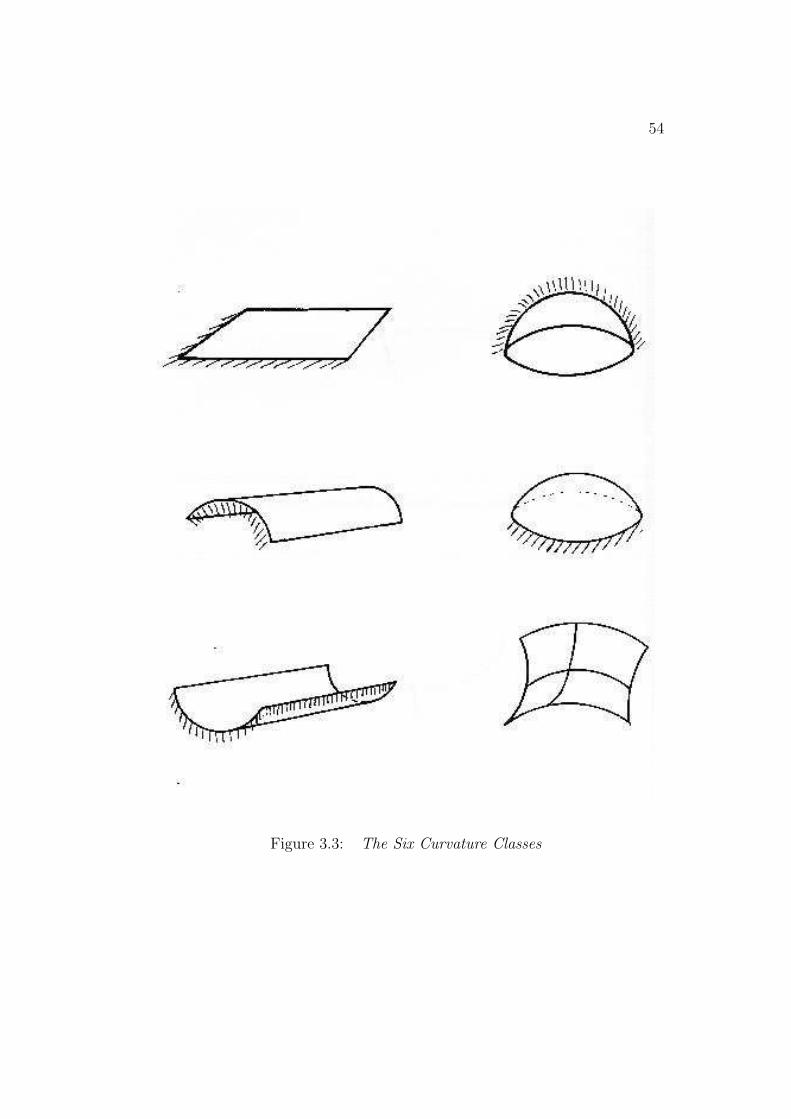
54

Figure 3.3: The Six Curvature Classes

55

Figure 3.4: Segmentation of a Sausage

The theoretical grounds for these conditions and how to achieve themare not settled, but the following general principles seem reasonable. Thesegmentation should produce connected regions of constant character withall curvature magnitudes roughly the same and in the same direction. Fur-ther, the segmentations should be stable to viewpoint and minor variationsin object shape, and should result in unique segmentations. Because thecriteria are object-centered, they give unique segmentation, independent ofviewpoint. As we can also apply the criteria to the models, model invo-cation (Chapter 8) and matching (Chapter 9) are simplified by comparingsimilar corresponding features. The examples used in this book were chosento be easily and obviously segmentable to avoid controversy. Thus, imageand model segmentations will have roughly corresponding surface regions,though precisely corresponding boundaries are not required.

Scale affects segmentation because some shape variations are insignificantwhen compared to the size of objects considered. In particular, less pro-nounced shape segmentations will disappear into insignificance as the scaleof analysis grows. No absolute segmentation boundaries exist on free-formobjects, so criteria for a reasonable segmentation are difficult to formulate.(Witkin [165] has suggested a stability criterion for scale-based segmentations

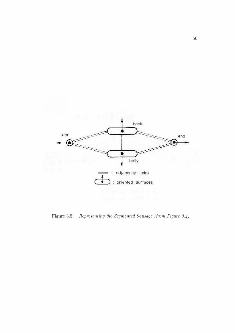
56

Figure 3.5: Representing the Segmented Sausage (from Figure 3.4)

57

of one dimensional signals.)This does not imply that the segmentation boundaries must remain con-

stant. For some ranges of scale, the sausage’s boundaries (Figure 3.4) willmove slightly, but this will not introduce a new segmented surface. Invoca-tion and matching avoid the boundary movement effects by emphasizing thespatial relationships between surfaces (e.g. adjacency and relative orienta-tion) and not the position of intervening boundaries.

Some research into surface segmentation has occurred. Brady et al. [40]investigated curvature-based local descriptions of curved surfaces, by con-structing global features (i.e. regions and lines of curvature) from localproperties (i.e. local principal curvatures). Besl [24] started with similarcurvature properties to seed regions, but then used numerical techniques tofit surface models to the data (e.g. to ellipsoidal patches) and grow largerpatches. This work was particularly effective. Hoffman and Jain [90] clus-tered surface normals to produce three types of patches (planar, convex andconcave). Patches were linked by four types of boundary (depth disconti-nuity, orientation discontinuity, tesselation and null). Null and tesselationboundaries were later removed to produce larger patches.

Following on from Besl’s work, Cai [43] has been investigating multiplescale segmentation of surface patches from range data. He used a modifieddiffusion smoothing process to blend the features and then forms surfacepatches from region growing based on local principal curvature estimates.Large features that remain over several scales are selected to form a stablerepresentation. Figure 3.6 shows an intermediate stage of the segmentationof a face, where the positive ellipsoidal regions are shown in white, hyper-boloidal regions are grey and negative ellipsoidal regions are black. Thoughthere is still considerable research on segmentation to be done, features suchas these are suitable for recognition with a coarse scale model.

Labeling

With the segmentation processes described above, the boundary labelingproblem becomes trivial. The purpose of the labeling is to designate whichboundaries result from the shape segmentations, and which result from occlu-sion. The type of a shape segmentation boundary is probably not important,as scale affects the labeling, so it is not used. However, the different types arerecorded for completeness and the shape of the boundary helps to identify

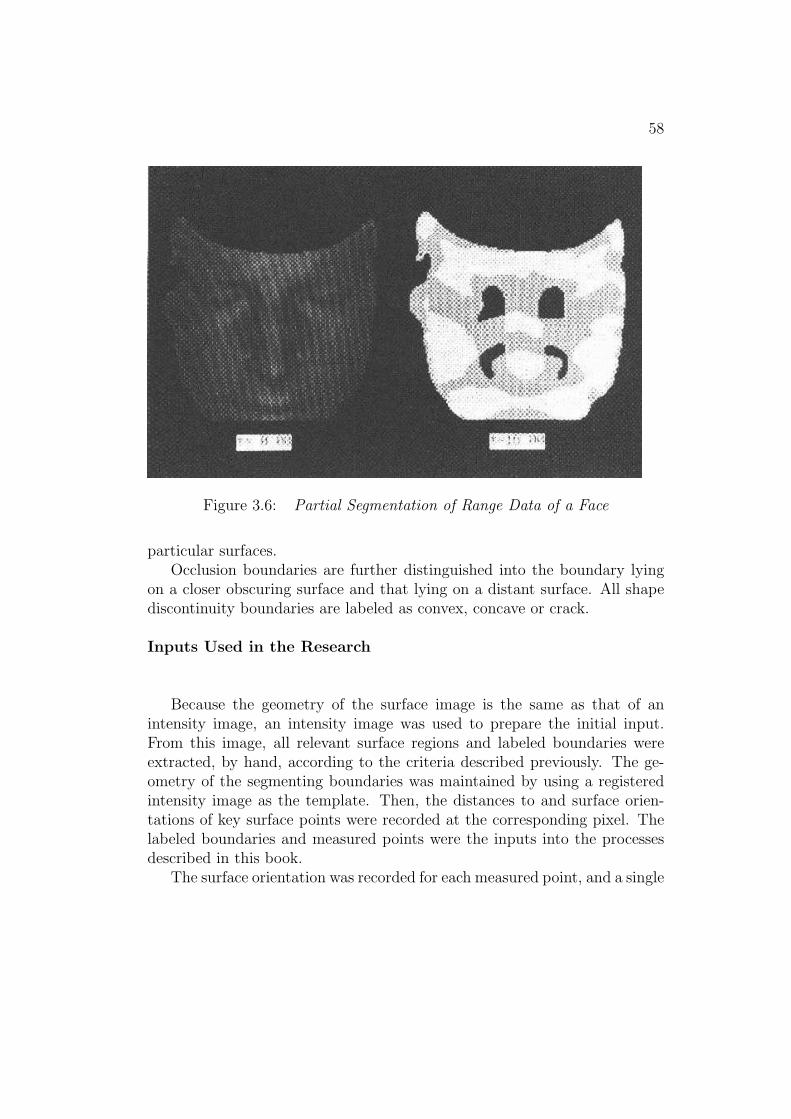
58

Figure 3.6: Partial Segmentation of Range Data of a Face

particular surfaces.Occlusion boundaries are further distinguished into the boundary lying

on a closer obscuring surface and that lying on a distant surface. All shapediscontinuity boundaries are labeled as convex, concave or crack.

Inputs Used in the Research

Because the geometry of the surface image is the same as that of anintensity image, an intensity image was used to prepare the initial input.From this image, all relevant surface regions and labeled boundaries wereextracted, by hand, according to the criteria described previously. The ge-ometry of the segmenting boundaries was maintained by using a registeredintensity image as the template. Then, the distances to and surface orien-tations of key surface points were recorded at the corresponding pixel. Thelabeled boundaries and measured points were the inputs into the processesdescribed in this book.

The surface orientation was recorded for each measured point, and a single

59

measurement point was sufficient for planar surfaces. For curved surfaces,several points (6 to 15) were used to estimate the curvature, but it turned outthat not many were needed to give acceptable results. As the measurementswere made by hand, the angular accuracy was about 0.1 radian and distanceaccuracy about 1 centimeter.

Those processes that used the surface information directly (e.g. for com-puting surface curvature) assumed that the distance and orientation infor-mation was dense over the whole image. Dense data values were interpolatedfrom values of nearby measured points, using a 1/R2 image distance weight-ing. This tended to flatten the interpolated surface in the region of the datapoints, but had the benefit of emphasizing data points closest to the testpoint. A surface approximation approach (e.g. [77]) would have been better.The interpolation used only those points from within the segmented surfaceregion, which was appropriate because the regions were selected for havinguniform curvature class.

We now show the input data for the test scene in greater detail. Figure1.1 showed the original test scene and Figure 1.4 showed the depth informa-tion coded so dark means further away. Figure 3.7 shows the y component ofthe unit surface normal. Here, brighter means more upward facing. Figure1.5 showed the occlusion label boundaries. Figure 3.8 shows the orientationdiscontinuity label boundaries and Figure 3.9 shows the curvature disconti-nuity boundary. Figure 3.10 shows the identifier assigned to each region andthe overall segmentation boundaries.

The Region Graph

The labeled, segmented surface image was represented as a graph, becauseit was compact and easily exploited key structural properties of the data.These are:

1. Regions are connected sets of surface points.

2. Boundary segments are connected sets of boundary points.

3. All points in one boundary segment have the same label.

4. Every region is totally bounded by a connected chain of boundary seg-ments.

60

Figure 3.7: Test Scene y Component of Surface Orientation

Figure 3.8: Test Scene Orientation Discontinuity Label Boundaries

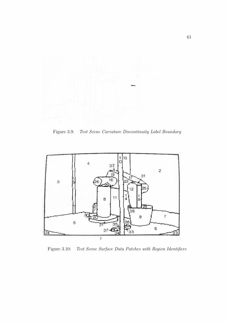
61

Figure 3.9: Test Scene Curvature Discontinuity Label Boundary

Figure 3.10: Test Scene Surface Data Patches with Region Identifiers

62

5. If one region is the front side of an obscuring boundary, the adjacentregion is the back side.

The resulting graph structure used nodes for the surface image regions andboundaries, and the links represented adjacency. The properties of this graphare:

1. Region nodes represent complete image regions.

2. Boundary nodes represent complete boundary segments.

3. Chains of boundary nodes represent connecting boundary segments.

4. Region nodes link to chains of boundary nodes that isolate them fromother regions.

5. Region nodes corresponding to adjacent regions have adjacency links.

The computation that makes this transformation is a trivial boundarytracking and graph linking process. No information is lost in the transforma-tions between representations, because of explicit linking back to the inputdata structures (even if there is some loss of information in the generalizationat any particular level). The only interesting point is that before tracking,the original segmented surface image may need to be preprocessed. The orig-inal image may have large gaps between identified surface regions. Beforeboundary tracking, these gaps have to be shrunk to single pixel boundaries,with corresponding region extensions. (These extensions have surface ori-entation information deleted to prevent conflicts when crossing the surfaceboundaries.) This action was not needed for the hand segmented test casesin this research.

3.2 Why Use Surfaces for Recognition?

It was Marr, who, in advocating the 212D sketch as an intermediate represen-

tation [112], brought surfaces into focus. Vision is obviously a complicatedprocess, and most computer-based systems have been incapable of copingwith both the system and scene complexity. The importance of Marr’s pro-posal lies in having a reconstructed surface representation as a significantintermediate entity in the image understanding process. This decision laidthe foundation for a theory of vision that splits vision into those processes

63

that contribute to the creation of the 212D sketch and those that use its

information.A considerable proportion of vision research is currently involved in gen-

erating the 212D sketch (or equivalent surface representations). This work

addresses the problem of what to do after the sketch is produced and somejustifications for and implications of using this surface information are dis-cussed in the sections below.

From What Sources Can We Expect to Get Surface Information?

The research presented here is based on the assumption that there willsoon be practical means for producing surface images. Several promising re-search areas suggest that this is likely, though none of the processes describedhere are “perfected” yet.

Direct laser ranging (e.g. [122, 98, 143]) computes surface depth by mea-suring time of flight of a laser pulse or by signal phase shift caused by pathlength differences. The laser is scanned over the entire scene, producing adepth image. Sonar range finding gives similar results in air, but has lowerresolution and has problems because of surface specularity.

Structured illumination uses controlled stimulation of the environment toproduce less ambiguous interpretations. One well known technique tracesthe scene with parallel light stripes ([147, 5, 133, 150, 127, 36]). The threedimensional coordinates of individual points on the stripes can be found bytriangulation along the baseline between the stripe source and sensor. Addi-tionally, this technique highlights distinct surfaces, because all stripes lyingon the same surface will have a similar character (e.g. all lines parallel), andusually the character will change radically at occlusion or orientation discon-tinuity boundaries. Analysis of stripe patterns may give further informationabout the local surface shape. Variations of this technique use a grey-codeset of patterns (e.g. [97]) or color coding ([99, 37]) to reduce the number ofprojected patterns.

A second technique uses one or more remotely sensed light spots. Byknowing the emitted and received light paths, the object surface can betriangulated, giving a depth image ([101, 132, 63]). The advantage of usinga spot is then there is no feature correspondence problem.

Besl [25] gives a thorough and up-to-date survey of the techniques andequipment available for range data acquisition.

64

Stereo is becoming a more popular technique, because it is a significantbiological process ([112, 113]) and its sensor system is simple and passive. Theprocess is based on finding common features in a pair of images taken fromdifferent locations. Given the relationship between the camera coordinateframes, the feature’s absolute location can be calculated by triangulation.

One major difficulty with this technique is finding the common feature inboth images. Biological systems are hypothesized to use (at least) pairededges with the same sign, and from the same spatial frequency channel([112, 113]). Other systems have used detected corners or points where signif-icant intensity changes take place ([54, 118]). More recently, researchers havestarted using trinocular (etc) stereo (e.g. [125]), exploiting a second epipo-lar constraint to reduce search for corresponding features and then producemore reliable pairings.

Another difficulty arises because stereo generally only gives sparse depthvalues, which necessitates surface reconstruction. This topic has only re-cently entered investigation, but some work has been done using a variety ofassumptions (e.g. [77, 158, 31]).

The relative motion of the observer and the observed objects, causescharacteristic flow patterns in an intensity image. These patterns can beinterpreted to acquire relative scene distance, surface orientation, rigid scenestructure and obscuring boundaries (in the viewer’s coordinate system), thoughthere is ambiguity between an object’s distance and velocity. From localchanging intensity patterns, it is possible to estimate the optic flow (e.g. fol-lowing [94, 120, 85]), from which one can then estimate information aboutthe objects in the scene and their motion (e.g. [136], [49, 106, 138]).

Shading, a more esoteric source of shape information well known toartists, is now being exploited by visual scientists. Horn [93] elaboratedthe theoretical structure for solving the “shape from shading” problem, andothers (e.g. [167, 129]) successfully implemented the theory for reasonablysimple, uniform surfaces. The method generally starts from a surface func-tion that relates reflectance to the relative orientations of the illumination,viewer and surface. From this, a system of partial differential equations isderived showing how local intensity variation is related to local shape vari-ation. With the addition of boundary, surface continuity and singular point(e.g. highlight) constraints, solutions can be determined for the system ofdifferential equations.

A major problem is that the solution relies on a global resolution of con-straints, which seems to require a characterized reflectance function for the

65

whole surface in question. Unfortunately, few surfaces have a reflectancefunction that meets this requirement, though Pentland [129] has shown rea-sonable success with some natural objects (e.g. a rock and a face), throughmaking some assumptions about the surface reflectance. There is also a prob-lem with the global convex/concave ambiguity of the surface, which ariseswhen only shading information is available, though Blake [32] has shown howstereo correspondence on a nearby specular point can resolve the ambiguity.For these reasons, this technique may be best suited to only qualitative orrough numerical analyses.

Variations of this technique have used multiple light sources ([50, 163])or polarized light [105]. Explicit surface descriptions (e.g. planar, cylindri-cal) have been obtained by examining iso-intensity contours [161] and fittingquadratic surfaces [45] to intensity data.

Texture gradients are another source of shape information. Assumingtexture structure remains constant over the surface, then all variation in ei-ther scale ([152, 130]) or statistics ([164, 124]) can be ascribed to surface slantdistortion. The measure of compression gives local slant and the direction ofcompression gives local tilt; together they estimate local surface orientation.

The final source of orientation and depth information comes from globalshape deformation. The technique relies on knowledge of how appearancevaries with surface orientation, how certain patterns create impressions ofthree dimensional structure, and what constraints are needed to reconstructthat structure. Examples of this include reconstructing surface orientationfrom the assumption that skew symmetry is slant distorted true symmetry[100], from maximizing the local ratio of the area to the square of the perime-ter [38], from families of space curves interpreted as geodesic surface markings[154], from space curves as locally circular arcs [21], and from characteris-tic distortions in known object surface boundary shapes [66]. Because thisinformation relies on higher level knowledge of the objects, these techniquesprobably would not help the initial stages of analysis much. However, theymay provide supporting evidence at the later stages.

There are variations in the exact outputs of each of these techniques, butmany provide the required data and all provide some form of useful threedimensional shape information. Further, some attributes may be derivablefrom measured values (e.g. orientation by locally differentiating depth).

How Can We Use Surface Information?

66

As the segmentation criteria are object-centered, the segments of thesurface image will directly correspond to model segments, especially sinceboundaries are mainly used for rough surface shape alignments. Makingthese symbolic correspondences means that we can directly instantiate andverify object models, which then facilitates geometric inversions of the imageformation process.

Surface orientation can then be used to simplify the estimation of theobject’s orientation. Given the model-to-data patch correspondences, pairingsurface normals leaves only a single rotational degree-of-freedom about thealigned normals. Estimating the object’s translation is also much simplerbecause the three dimensional coordinates of any image point (relative to thecamera) can be deduced from its pixel position and its depth value. Hence,the translation of a corresponding model point can be directly calculated.

All together, the surface information makes explicit or easily obtainablefive of the six degrees-of-freedom associated with an individual surface point(though perhaps imprecisely because of noise in the surface data and prob-lems with making precise model-to-data feature correspondences).

Depth discontinuities make explicit the ordering relationships with moredistant surfaces. These relationships help group features to form contextsfor model invocation and matching, and help verify potential matches, hencesimplifying and strengthening the recognition process.

Surface orientation allows calculation of the surface shape class (e.g. pla-nar, singly-curved or doubly-curved), and correction of slant and curvaturedistortions of perceived surface area and elongation. The relative orientationsbetween structures give strong constraints on the identity of their superobjectand its orientation. Absolute distance measurements allow the calculation ofabsolute sizes.

How Can Surface Data Help Overcome Current Recognition Prob-lems?

Recognizing real three dimensional objects is still difficult, in part becauseof difficulties with selecting models, matching complicated shapes, dealingwith occlusion, feature description, reducing matching complexity and copingwith noise. Surface information helps overcome all of these problems, asdiscussed below.

67

Selecting the correct model from the model database requires a descrip-tion of the data suitable for triggering candidates from the model base.Since descriptions of the model features are given in terms of their threedimensional shapes, describing data features based on their three dimen-sional shapes reduces the difficulties of comparison, and hence leads to moresuccessful model invocation.

Most current recognition programs have not progressed much beyondrecognizing objects whose shapes are largely block-like. One cause of thishas been a preoccupation with orientation discontinuity boundaries, which,though easier to detect in intensity images, are noticeably lacking on manyreal objects. Using the actual surfaces as primitives extends the range ofrecognizable objects. Faugeras and Hebert [63] demonstrated this by usingplanar patch primitives to successfully detect and orient an irregularly shapedautomobile part.

Viewed objects are often obscured by nearer objects and the ensuing lossof data causes recognition programs to fail. Surface images provide extrainformation that help overcome occlusion problems. For example, occlusionboundaries are explicit, and thus denote where relevant information stops.Moreover, the presence of a closer surface provides evidence for why theinformation is missing, and hence where it may re-appear (i.e. on the “otherside” of the obscuring surface).

Surface patches are less sensitive to fragmentation, because pixel connec-tivity extends in two dimensions. Describing the surfaces is also more robust,because (usually) more pixels are involved and come from a more compactarea. Globally, connectivity (i.e. adjacency) of surfaces is largely guaranteed,and slight variations will not affect description. Hence, the topology of themajor patches should be reliably extracted.

Establishing model-to-data correspondences can be computationally ex-pensive. Using surface patches helps reduce the expense in two ways: (1)there are usually fewer surface patches than, for example, the boundary seg-ments between them and (2) patch descriptions are richer, which leads toselecting fewer locally suitable, but globally incorrect model-to-data featurepairings (such as those that occur in edge-based matching algorithms).

Noise is omnipresent. Sensor imperfections, quantization errors, randomfluctuations, surface shape texture and minor object imperfections are typi-cal sources of data variation. A surface image segment is a more robust dataelement, because its size leads to reduced data variation (assuming O(n2)data values as compared with O(n) for linear features). This contrasts with

68

linear feature detection and description processes, in which noise can causeerroneous parameter estimates, loss of connectivity or wandering.

Why Not Use Other Representations?

There are three alternative contenders for the primary input data repre-sentation: edges, image regions and volumes.

Edges have been used extensively in previous vision systems. The keylimitations of their use are:

• ambiguous scene interpretation (i.e. whether caused by occlusion, shad-ows, highlights, surface orientation discontinuities or reflectance changes),

• ambiguous model interpretation (i.e. which straight edge of length 10could it be?),

• loss of data because of noise or low contrast, and

• image areas free from edges also contain information (e.g. shading).

While these limitations have not deterred research using edge-based recogni-tion, considerable difficulties have been encountered.

Image regions are bounded segments of an intensity image. Their mean-ing, however, is ambiguous and their description is not sufficiently relatedto three dimensional objects. For example, Hanson and Riseman [84] andOhta [123] segmented green image regions for tree boughs using color, yetthere is no reason to assume that trees are the only green objects in thescene nor that contiguous green regions belong to the same object. Further,the segmentations lose all the detailed structure of the shape of the bough,which may be needed to identify the type of tree. They augmented the roughclassification with general context relations, which assisted in the interpre-tation of the data. While this type of general information is important anduseful for scene analysis, it is often insufficiently precise and object-specificfor identification, given current theories of image interpretation.

Volumetric primitives seem to be useful, as discussed by Marr [112] andBrooks [42] in their advocation of generalized cylinders. These solids areformed by sweeping a cross-section along an axis and represent elongatedstructures well. For volumes with shapes other than something like general-ized cylinders (e.g. a head), the descriptions are largely limited to explicit

69

space-filling primitives, which is insufficiently compact, nor does it have thepower to easily support appearance deductions.

The generalized cylinder approach also leads to problems with relatingvolumetric features to observed visible surface data, because there is no sim-ple transformation from the surface to the solid under most representations.Marr [112] showed that generalized cylinders were a logical primitive becausethese are the objects with planar contour generators from all points of view(along with a few other conditions) and so are natural interpretations forpairs of extended obscuring boundaries. Unfortunately, few objects meet theconditions. Moreover, this transformation ignored most of the other informa-tion available in the 21

2D sketch, which is too useful to be simply thrown away.

Final Comments

This completes a quick review of why surface information is useful, howone might obtain the data, and how it might be segmented for use. The nextchapter starts to use the data for the early stages of scene analysis.

Chapter 4

Making Complete SurfaceHypotheses

The first step in the interpretation of surface information is the formationof surface hypotheses, which groups surface image regions to form completesurfaces of the unidentified objects. This is the first important transforma-tion from image-based data to object-based data. Further, it reduces datacomplexity by representing one or more surface regions by a single symbolicentity.

If segmentation has been successful, then the surface image regions shouldclosely correspond to the visible portions of the object’s surface patches.Three problems may cause the patches to not correspond closely:

1. A data patch may correspond to several object surface patches, becauseof segmentation failure.

2. The object surface patch may be fragmented into several data patches,because of segmentation failure.

3. The object surface patch may be fragmented or smaller because ofocclusion.

The first two problems are a concern for segmentation and are not consideredclosely here, though some corrective action is possible once a model has beenselected (e.g. a predicted model SURFACE can be used to guide splitting ormerging of patches). The third problem is the main concern of this chapter,which shows that the most common cases of occlusion can be overcome withthe surfaces largely reconstructed.

70

71

Because of the pervasiveness of occlusion in natural scenes, this recon-struction is necessary. Reconstructed surfaces can only be hypothetical but,by the surface segmentation assumptions (Chapter 3), there are no extremesurface or boundary shape variations in a single segment. As many naturalobject boundaries exhibit surface smoothness over moderate distances (atappropriate scales), reconstruction should be possible. This is even morelikely with most man-made objects.

Some research has tried to overcome occlusion directly by using visiblecues. Guzman [81] used paired TEE junctions to signal the presence of oc-clusion and locate which two dimensional image regions should be connected.Adler [3] also used TEE information to infer depth ordering between scenefeatures. The key problem is detection of occlusion, and their work reliedon the use of TEE detections, which show where one surface boundary isabruptly terminated by the obscuring boundary of a closer surface. Becausea fragmented obscured surface must have a pair of TEEs at the start andend of the obscuring boundary (under normal circumstances), the detectionof a matched pair of TEEs suggests a likely occlusion boundary, and hencewhere the invisible portion of the surface lies. In the research described here,occlusion boundaries are directly labeled, so the occlusion cueing processis no longer necessary. The TEEs are still useful for signaling where alongthe occlusion boundary the obscured surfaces’ boundaries terminate. Theywould also be useful for helping cope with missing, incorrect or ambiguousdata (e.g. when a correct boundary label is not available).

4.1 Reconstructing Obscured Surfaces

This process starts with the region graph described in Chapter 3. Initially,the surface hypotheses are identical to the image regions. From these, largersurface hypotheses are created based on surface extensions consistent withpresumed occlusions. While it is obviously impossible to always correctlyreconstruct obscured structure, often a single surface hypothesis can be cre-ated that joins consistent visible surface parts. Figure 4.1 shows a simplecase of surface reconstruction.

In Figure 4.2, four cases of a singly obscured surface are shown, along withthe most reasonable reconstructions possible, where the boundary arrowsindicate an occlusion boundary with the object surface on the right of thearrow and the obscuring surface on the left. In the first case, the original

72

Figure 4.1: Surface Hypothesis Construction Process

surface boundaries meet when they are extended, and this is presumed toreconstruct a portion of the surface. If the boundaries change their curvatureor direction, then reconstruction may not be possible, or it may be erroneous.(Even if erroneous, the reconstructed surface may more closely approximatethe true surface than the original input.) The second case illustrates whenreconstruction does not occur, because the unobscured boundaries do notintersect when extended. The third case shows an interior obscuring objectremoved. The fourth case shows where the surface has been split by anobscuring object and reconstructed. The label of the boundary extensionalways remains back-side-obscuring, because it might participate in furtherreconstructions.

What is interesting is that only three rules are needed for the reconstruc-tion (see Figure 4.3). They are:

1. remove interior closer surfaces (Rule 1),

2. extend and connect boundaries on separate surface hypotheses to forma single surface hypothesis (Rule 2), and

3. extend and connect boundaries on a single surface to make a largersurface (Rule 3).

Rule 2 connects two separated surfaces if either extension of the bound-aries intersect. The remaining portion of the obscuring boundary is discon-nected to indicate no information about the obscured portion of the surface

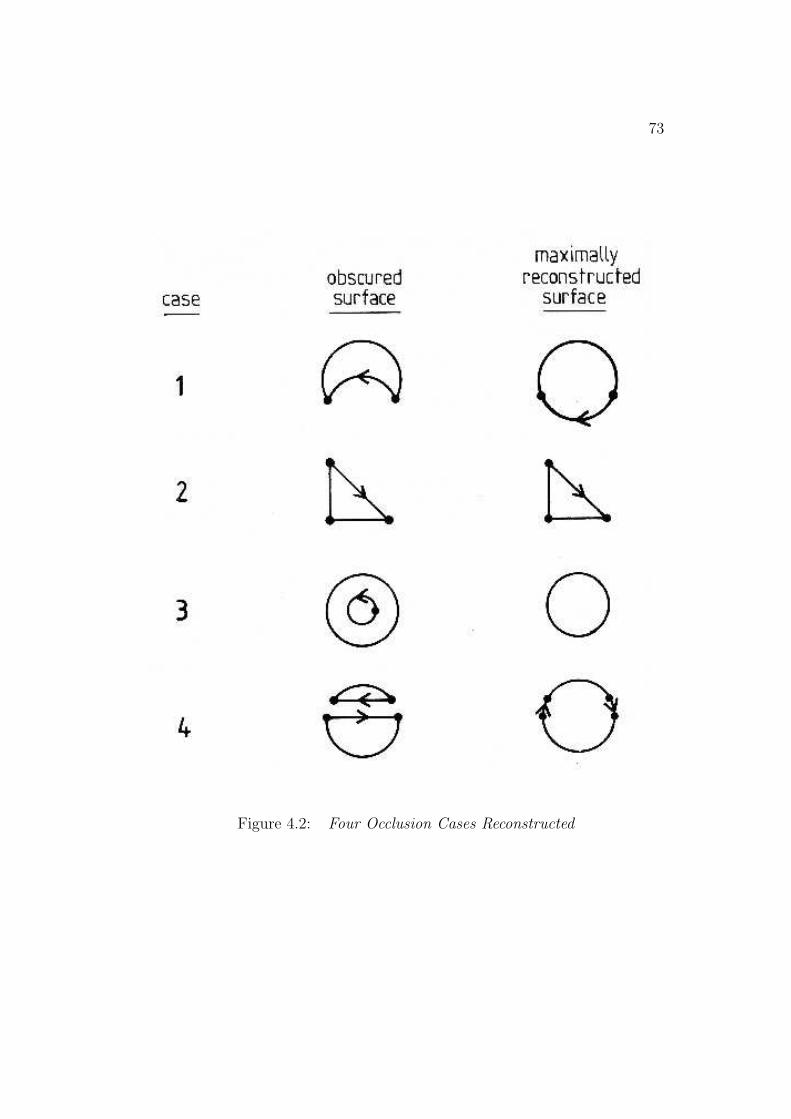
73

Figure 4.2: Four Occlusion Cases Reconstructed

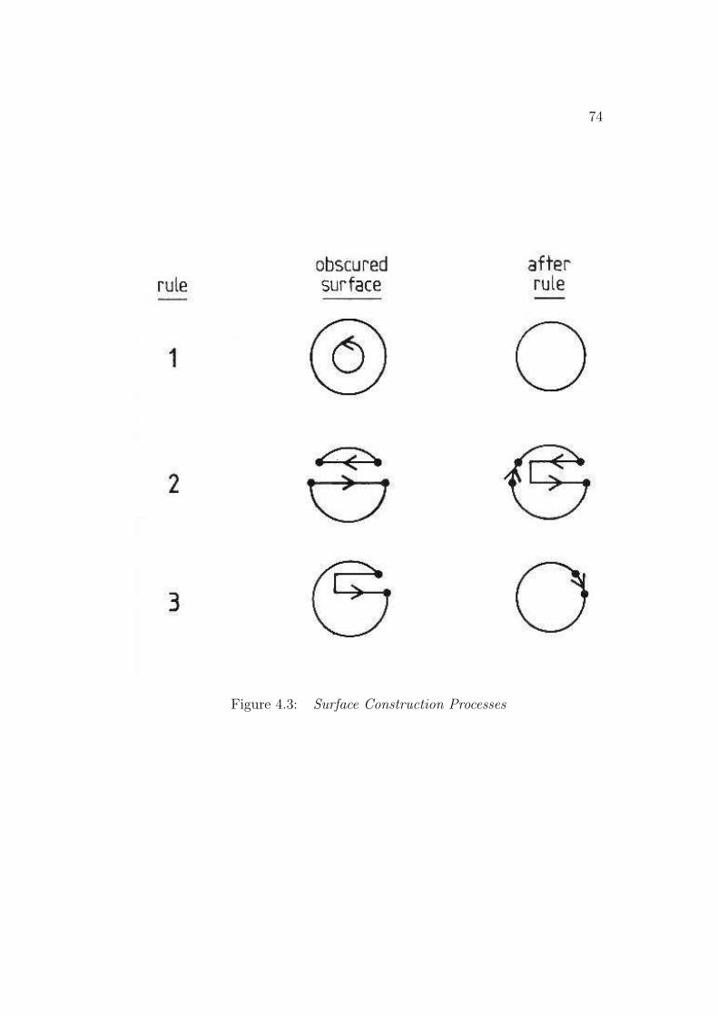
74

Figure 4.3: Surface Construction Processes

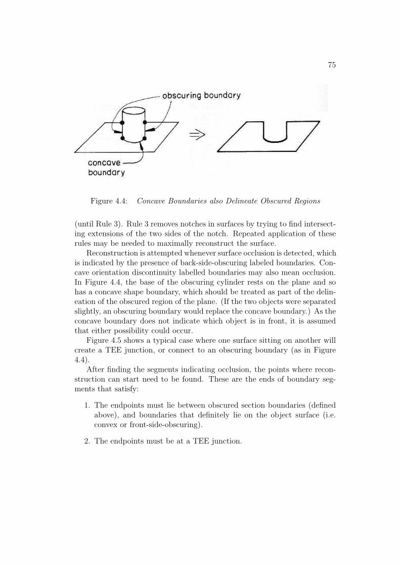
75

Figure 4.4: Concave Boundaries also Delineate Obscured Regions

(until Rule 3). Rule 3 removes notches in surfaces by trying to find intersect-ing extensions of the two sides of the notch. Repeated application of theserules may be needed to maximally reconstruct the surface.

Reconstruction is attempted whenever surface occlusion is detected, whichis indicated by the presence of back-side-obscuring labeled boundaries. Con-cave orientation discontinuity labelled boundaries may also mean occlusion.In Figure 4.4, the base of the obscuring cylinder rests on the plane and sohas a concave shape boundary, which should be treated as part of the delin-eation of the obscured region of the plane. (If the two objects were separatedslightly, an obscuring boundary would replace the concave boundary.) As theconcave boundary does not indicate which object is in front, it is assumedthat either possibility could occur.

Figure 4.5 shows a typical case where one surface sitting on another willcreate a TEE junction, or connect to an obscuring boundary (as in Figure4.4).

After finding the segments indicating occlusion, the points where recon-struction can start need to be found. These are the ends of boundary seg-ments that satisfy:

1. The endpoints must lie between obscured section boundaries (definedabove), and boundaries that definitely lie on the object surface (i.e.convex or front-side-obscuring).

2. The endpoints must be at a TEE junction.

76

Figure 4.5: TEE Junctions Delimit Reconstruction Concave Boundaries

3. The true object surface boundary must be the shaft of the TEE.

These points are illustrated in Figure 4.6.For reconstruction, boundary segments must intersect when extended. As

intersecting three dimensional surface curves still intersect when projectedonto the image plane, extension and intersection is done only in two dimen-sions, thus avoiding the problems of three dimensional curve intersection.Extending the boundaries is done by estimating the curvature shortly be-fore the terminating TEE and projecting the curve through the TEE. Onthe basis of the boundary segmentation assumptions (Chapter 3), segmentscan be assumed to have nearly constant curvature, so the extension processis justified. Segments that intersect in two dimensions can then be furthertested to ensure three dimensional intersection, though this was not neededwhen using the additional constraints given below. Further, because of nu-merical inaccuracies in the range data, three dimensional intersection is hardto validate.

To prevent spurious reconstructions that arise in complex scenes withmany obscuring objects, other constraints must be satisfied:

• If a portion of a surface is obscured, then that portion must be com-pletely bounded by an appropriate type of boundary (as defined above).

• The ends of the unobscured portions of the surface boundary must bejoinable.

• The joined portions of surface must lie on the same side of the boundaryextension.

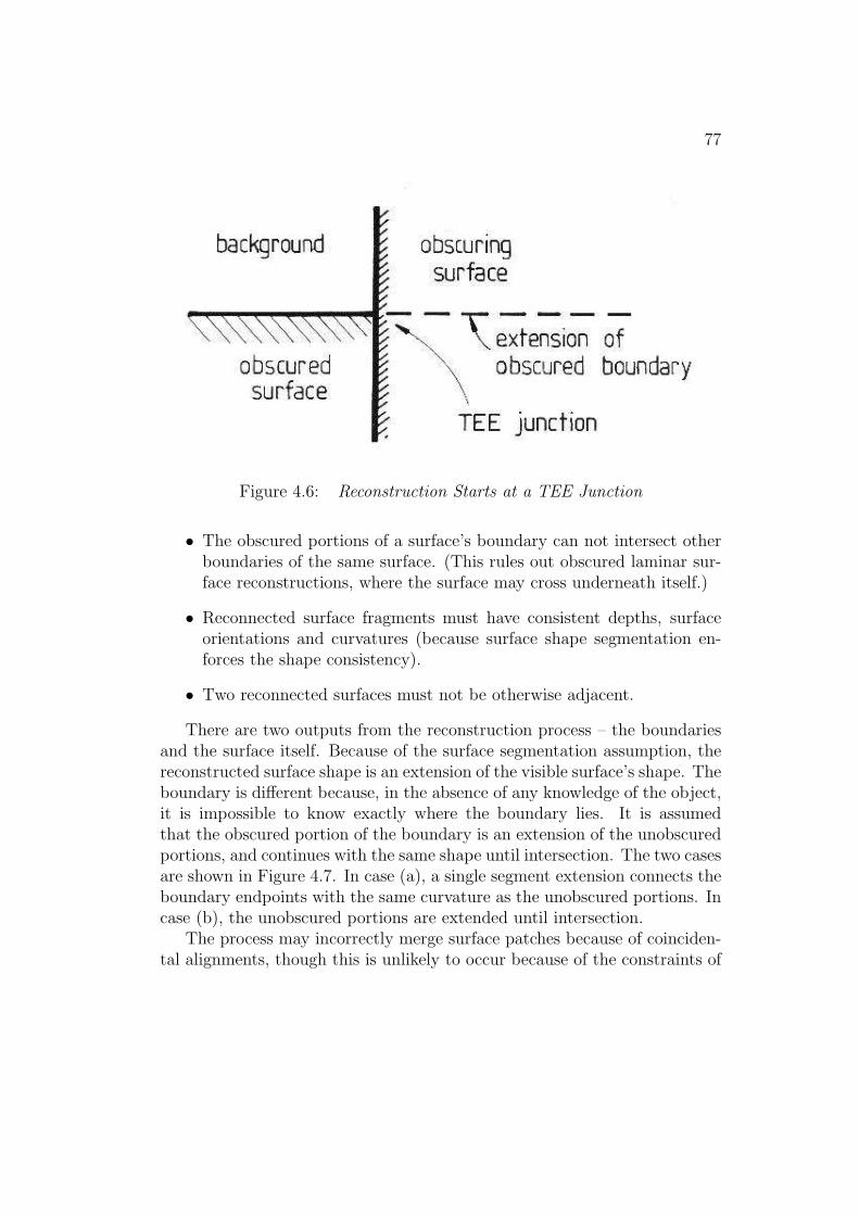
77

Figure 4.6: Reconstruction Starts at a TEE Junction

• The obscured portions of a surface’s boundary can not intersect otherboundaries of the same surface. (This rules out obscured laminar sur-face reconstructions, where the surface may cross underneath itself.)

• Reconnected surface fragments must have consistent depths, surfaceorientations and curvatures (because surface shape segmentation en-forces the shape consistency).

• Two reconnected surfaces must not be otherwise adjacent.

There are two outputs from the reconstruction process – the boundariesand the surface itself. Because of the surface segmentation assumption, thereconstructed surface shape is an extension of the visible surface’s shape. Theboundary is different because, in the absence of any knowledge of the object,it is impossible to know exactly where the boundary lies. It is assumedthat the obscured portion of the boundary is an extension of the unobscuredportions, and continues with the same shape until intersection. The two casesare shown in Figure 4.7. In case (a), a single segment extension connects theboundary endpoints with the same curvature as the unobscured portions. Incase (b), the unobscured portions are extended until intersection.

The process may incorrectly merge surface patches because of coinciden-tal alignments, though this is unlikely to occur because of the constraints of

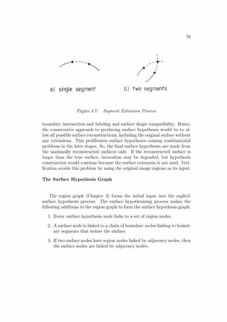
78

Figure 4.7: Segment Extension Process

boundary intersection and labeling and surface shape compatibility. Hence,the conservative approach to producing surface hypotheses would be to al-low all possible surface reconstructions, including the original surface withoutany extensions. This proliferates surface hypotheses causing combinatorialproblems in the later stages. So, the final surface hypotheses are made fromthe maximally reconstructed surfaces only. If the reconstructed surface islarger than the true surface, invocation may be degraded, but hypothesisconstruction would continue because the surface extension is not used. Veri-fication avoids this problem by using the original image regions as its input.

The Surface Hypothesis Graph

The region graph (Chapter 3) forms the initial input into the explicitsurface hypothesis process. The surface hypothesizing process makes thefollowing additions to the region graph to form the surface hypothesis graph:

1. Every surface hypothesis node links to a set of region nodes.

2. A surface node is linked to a chain of boundary nodes linking to bound-ary segments that isolate the surface.

3. If two surface nodes have region nodes linked by adjacency nodes, thenthe surface nodes are linked by adjacency nodes.

79

Figure 4.8: Surface Hypotheses for the Test Scene

4.2 Examples from the Test Scenes

Figure 3.10 showed the initial image regions and Figure 4.8 shows the finalsurface hypotheses formed by the processes described in this chapter (num-bers in the picture are the surface index).

There are several instances of successful surface reconstructions. Figure4.9 shows reconstruction of the robot upper arm side panel. The surfacemerging operation has rejoined the two sections, and the boundary extensionhas largely restored the missing section in the lower left corner. Because thereconstruction is only suggestive, and because the leftmost boundary wasnot observed as being curved, the reconstruction is a little generous andslightly exceeds the actual surface. The right end of the panel could not bereconstructed because of insufficient evidence for the true boundary, althoughthe labeling claimed it was obscured. Other valid reconstructions includedthe block lying on the table and the two halves at the back of the trash can(Figure 4.10). The latter is interesting because it was a curved surface, somatching of surface shape had to account for the change in orientation. Oneinappropriate merging occurred: the two top panels of the robot upper arm

80

Figure 4.9: Observed and Reconstructed Upper Arm Surface

had their real join hidden behind the vertical gantry column. As they werecontinuous, their orientation differed only slightly, and met all the occlusionconstraints, they were merged as well. The hypothesis construction processexpects this type of error, so it did not prove catastrophic.

These examples show that the obscured surface reconstructions are suc-cessful, and Figure 4.8 shows that most reasonable surfaces are made.

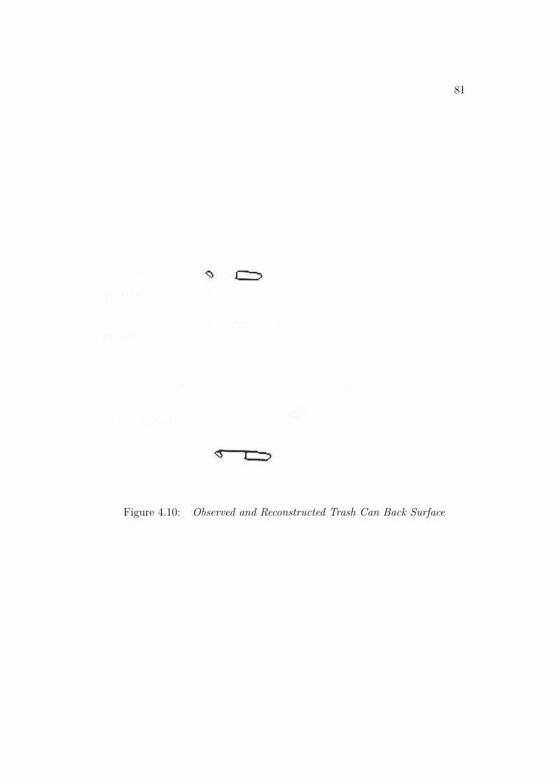
81

Figure 4.10: Observed and Reconstructed Trash Can Back Surface

82

Figure 4.11: Unsuccessful Extensions

4.3 Discussion

The major problem with the surface reconstruction constraints is unsolvable– one cannot reconstruct the invisible when the image is taken from a singleviewpoint. Some examples are seen in Figure 4.11. In the first case, theextended segments never intersect, and in the second, extension creates alarger, incorrect surface. Stereo or observer movement might help reconstructthe surface, however. Feature regularity (such as symmetry) might also beexploited to aid reconstruction. As the goal was to reconstruct enough toallow the rest of recognition to proceed, a few failures should be acceptable.

Another obvious criticism is over performance when applied to rich nat-ural images. Realistic images are likely to have missing or erroneous data,such as for line labels or surface orientation, which is likely to degrade boththe quality and rate of performance. In short, the processes described in thischapter seem fine for clear laboratory images, but it is hard to predict theirperformance on natural scenes.

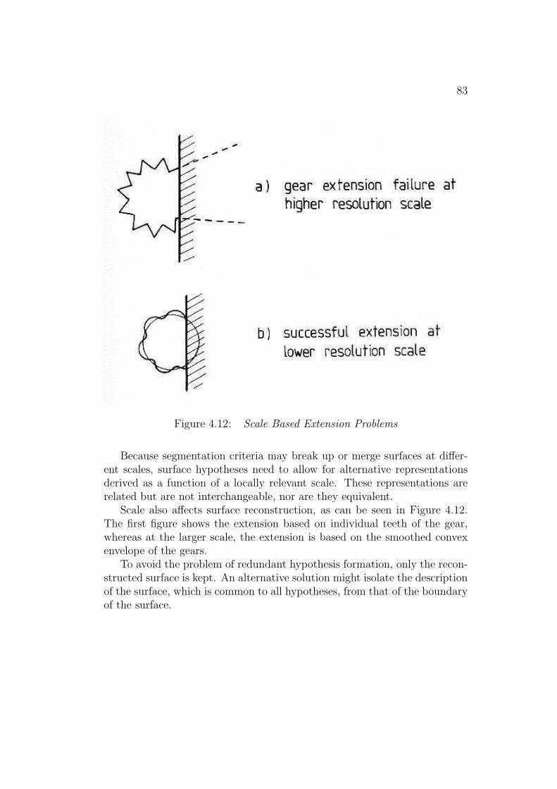
83

Figure 4.12: Scale Based Extension Problems

Because segmentation criteria may break up or merge surfaces at differ-ent scales, surface hypotheses need to allow for alternative representationsderived as a function of a locally relevant scale. These representations arerelated but are not interchangeable, nor are they equivalent.

Scale also affects surface reconstruction, as can be seen in Figure 4.12.The first figure shows the extension based on individual teeth of the gear,whereas at the larger scale, the extension is based on the smoothed convexenvelope of the gears.

To avoid the problem of redundant hypothesis formation, only the recon-structed surface is kept. An alternative solution might isolate the descriptionof the surface, which is common to all hypotheses, from that of the boundaryof the surface.

84

Final Comments

The test image shows that we can expect substantial occlusion in threedimensional scenes. This chapter demonstrates that much of the lost infor-mation can be inferred from the physical and modeling constraints, withoutgenerating many errors or redundant hypotheses.

Chapter 5

Surface Clusters

A competent object recognition system needs a perceptual organization mech-anism, to both indicate which image features are related and delimit theobject’s spatial extent. To help provide this mechanism, we developed [69]a new intermediate representation, surface clusters, lying between the seg-mented surface image and the model-based three dimensional object hypothe-ses. This chapter describes their role in the IMAGINE I system.

5.1 Why Surface Clusters?

A surface cluster is a set of surface patches isolated by suitable boundaries.The goal of the surface cluster formation process is to produce a volumetricimage representation for portions of the scene that might be identifiable threedimensional objects. There are three motivations for this:

1. the creation of a volumetric intermediate representation suitable foridentity-independent operations,

2. the focusing of attention on an object and its associated image featuresand

3. the reduction of search complexity through structuring the image fea-tures.

The first motivation for a surface cluster is a competence issue – sur-face clusters are new representations that bridge the conceptual distancebetween the segmented surface image and the object. The point is to create

85

86

an “unidentified, but distinct” object interpretation associated with sets ofimage features – a volumetric representation describing solid objects with ap-proximate spatial relationships but without identifications. With this struc-ture, the key image understanding representations now become (followingMarr [112]): image – primal sketch – 21

2D sketch – surface clusters – objects.

The grouping creates a good starting point for further interpretation; it is aform of figure/ground separation for solid objects.

Such representations are needed for unidentifiable objects to allow inter-mediate levels of image interpretation even when full identification is notachieved, whether because of faults or lack of models in the database. Pos-sible application areas include vehicle navigation, collision avoidance, objecttracking or grasping.

The second motivation is to partition the image features into activitycontexts for the later stages of recognition. This will help to focus sceneunderstanding to make more obvious the interpretation of a group of imagefeatures and how they are matched with a model. By eliminating irrele-vant and unrelated image features, it should be easier to identify and verifyobjects, since only features belonging to a single object will be present.

The “context” aspect of surface clusters is exploited by model invoca-tion (Chapter 8) and hypothesis construction (Chapter 9). Model invocationrequires contexts within which to accumulate evidence to hypothesize mod-els, and surface clusters are ideal for invoking the volumetric models (theASSEMBLY – see Chapter 7). To help fully instantiate an ASSEMBLY hy-pothesis, it may be necessary to search for additional evidence. Because AS-SEMBLY invocation has occurred in a surface cluster context, any additionalstructural evidence should also come from the context. Thus, processing hasbeen focused to a distinct region of the image.

The final motivation for creating these aggregations is one of performance– eliminating unrelated image features produces an immediate reduction inthe complexity of the scene analysis. The whole interpretation has beenreduced to a set of smaller independent problems, which is necessary giventhe quantity of data in an image.

A casual mathematical analysis supports this point. Here, we are mainlyconcerned with intersurface relationships (i.e. relative surface orientationand matching data surfaces to model SURFACEs). Since every surface onan object has a relationship to every other surface on the object, an objectwith N visible surfaces has O(N2) relationships. If there are A objects in thescene, each with B visible surfaces, there will be AB total visible surfaces.

87

So, initially, the analysis complexity is O((AB)2). However, if the surfacecluster process succeeds in partitioning the image into the A objects, thenthe complexity is reduced to O(AB2). For typical scenes, a nominal valuefor A is 20, so this can lead to a substantial improvement in performance.

5.2 Theory of Surface Clusters

The goal of the surface cluster formation process is to isolate the visibleportion of each distinct three dimensional object’s surface, so that later stagesof the scene analysis can associate a model with the surface cluster.

The primary input into the process is the set of surface hypotheses pro-duced as output of the processes described in Chapter 4. The surface hy-potheses are linked by adjacency, and relative surface orientation at theboundaries is known.

The output of the process is a set of surface clusters hierarchically linkedby inclusion, with each consisting of a set of surface patches. Though thesurface cluster is not closed (i.e. it is missing the back side), it defines a solidbounded in front by the visible surfaces.

The surface cluster formation process is closely linked to the model struc-ture known as the ASSEMBLY, which is defined in Chapter 7. The ASSEM-BLY is a model of a three dimensional solid and is composed of SURFACEsor recursively defined subcomponents. Properties we would like the surfacecluster formation process to have are:

• Every model ASSEMBLY is wholly contained in at least one surfacecluster.

• There are surface clusters containing only a single primitive model AS-SEMBLY.

• Only complete ASSEMBLYs are contained in surface clusters.

• There is a hierarchy of surface clusters corresponding to the hierarchyof model ASSEMBLYs.

However, at this stage of image analysis, models are not available to helpsegment the image, nor is the model base known. Hence, to achieve ourgoal with these properties, two assumptions must be made about the modelstructure independent of the actual models:

88

• If a set of model SURFACEs is completely surrounded by a set ofconcave or crack surface boundaries, then they are modeled as a distinctASSEMBLY.

• If two model SURFACEs are adjacent across a convex surface boundary,then they are in the same model ASSEMBLY.

For example, a nose on a face, or a handle on a coffee cup would thus be inseparate ASSEMBLYs.

The process of creating the surface clusters has three steps:

1. Classify adjacent surface regions as connected or unconnected.

2. Form primitive surface clusters from connected groups of surfaces. (Prim-itive surface clusters are those that cannot be split further.)

3. Merge primitive surface clusters to form larger surface clusters.

These steps are described in detail below.The algorithm is conservative, in that it tries to avoid splitting the small-

est model ASSEMBLYs between surface clusters at the price of creatingclusters containing several ASSEMBLYs. Splitting an object between sev-eral different surface clusters would be catastrophic because it asserts thatthe segregated components are unrelated. Creating clusters larger than singleobjects is mainly an annoyance, because the rest of the recognition processthen has more work to identify the objects.

Determining Surface Connectivity

The segmented surface image can be thought of as a graph, where thenodes of the graph represent the surface patches and the arcs of the graphrepresent surface adjacency. These arcs will be labeled as connecting or seg-menting, according to criteria based on boundary type and configuration.The connection criteria are simple and logical, except for a laminar surfacecase (described shortly) and are based on obvious three dimensional proper-ties of surface connectivity and object depth ordering. Splitting the graph atsegmenting boundaries partitions the scene into sets of connected surfaces –forming the primitive surface clusters.

89

We assume that the modeled objects are segmented into subcomponentsat chains of connected concave boundaries. As concave model boundaries areobserved as concave image boundaries, the latter are potentially segmenting.In Figure 5.1 part (a), the concave boundary is truly segmenting.

Further, distinct objects are often on opposite sides of concave surfaceorientation boundaries. For example, a block sitting on a table has concaveboundaries isolating it from the table. Nameable subcomponents of naturalobjects often fit flushly with concave boundaries, as in the nose-to-face junc-tion. Because the boundary is concave, it is indeterminate whether the twosurfaces are joined or merely in contact. Moreover, it is usually impossible totell which surface passes underneath the other past the point of the observedconcave boundary. So, the conservative approach suggests that this bound-ary causes a segmenting arc. Assuming concave boundaries necessarily implysegmentation leads to contradictions as seen in Figure 5.1 part (b), wherethere is no reasonable shape boundary at point X to continue segmentation.If there are other connections between the two surfaces that do not involve asegmenting boundary, then the final surface cluster will include both surfaces.

A more complicated case occurs with crack-type boundaries. Here, twosurfaces may be coincidentally aligned, or part of a flush contact boundary(as often occurs with revolute joints). Because of the ambiguity, it is assumedthat connectivity does not hold across crack-type joints.

Whenever one object sits in front of or on top of another, the interveningboundary is always either concave or obscuring, as illustrated in Figure 5.2.To complete the isolation of the cylinder in part (a) from the backgroundplane, a rule is needed to handle obscuring boundaries. As these usuallygive no clues to the relation between opposing surfaces (other than beingdepth separated), surfaces will usually be segmented across these, and sosegmenting arcs join the nodes representing these surfaces.

Connectivity holds across some obscuring boundaries. Disregarding co-incidental alignments, the one exception found occurs when laminar objectsfold back on themselves, as illustrated in Figure 5.3. This figure shows a leaffolded over and the two surfaces of a trash can. The arrows on the boundarymean that it is an obscuring type boundary with (here) the front surfacelying to the left when looking along the boundary in the direction of the ar-row. In both cases, the two surfaces are connected, even though an obscuringboundary intervenes, and so here a connecting arc is used. Fortunately, thiscase has a distinctive signature: the arrow vertices shown at the right side

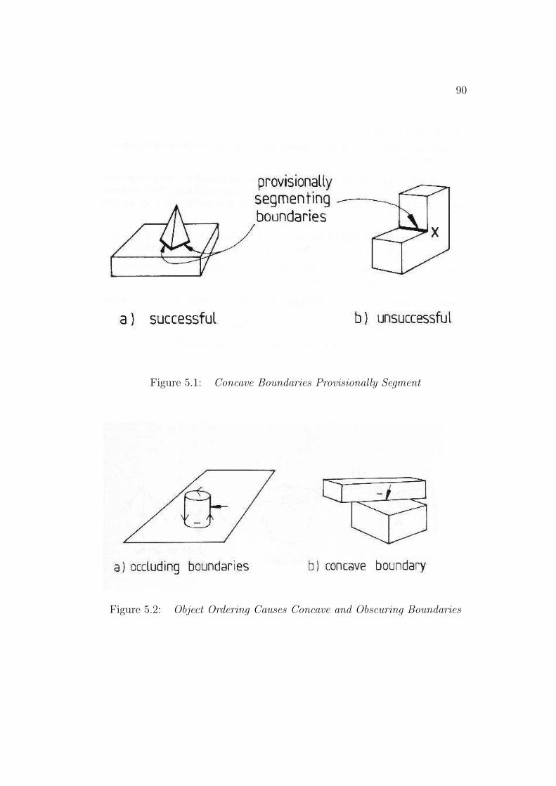
90

Figure 5.1: Concave Boundaries Provisionally Segment

Figure 5.2: Object Ordering Causes Concave and Obscuring Boundaries

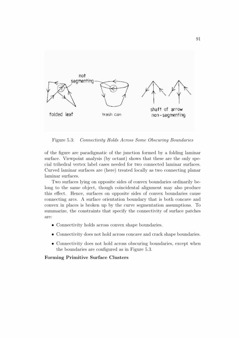
91

Figure 5.3: Connectivity Holds Across Some Obscuring Boundaries

of the figure are paradigmatic of the junction formed by a folding laminarsurface. Viewpoint analysis (by octant) shows that these are the only spe-cial trihedral vertex label cases needed for two connected laminar surfaces.Curved laminar surfaces are (here) treated locally as two connecting planarlaminar surfaces.

Two surfaces lying on opposite sides of convex boundaries ordinarily be-long to the same object, though coincidental alignment may also producethis effect. Hence, surfaces on opposite sides of convex boundaries causeconnecting arcs. A surface orientation boundary that is both concave andconvex in places is broken up by the curve segmentation assumptions. Tosummarize, the constraints that specify the connectivity of surface patchesare:

• Connectivity holds across convex shape boundaries.

• Connectivity does not hold across concave and crack shape boundaries.

• Connectivity does not hold across obscuring boundaries, except whenthe boundaries are configured as in Figure 5.3.

Forming Primitive Surface Clusters

92

Primitive surface clusters are formed by collecting all surface patch nodesthat are directly or transitively connected in the graph, once all arcs are la-beled as “segmenting” or “connecting”. Thus, image features that can onlybelong to the same object lie in the same surface cluster, and features thatpossibly belong to other objects do not lie in the cluster.

Depth Merged Surface Clusters

The goal of the surface cluster process is to associate all components ofan object in some surface cluster. All components of a model may not occurin the same primitive surface cluster for several reasons:

• The object may consist of several subcomponents, each of which ap-pears in smaller surface clusters.

• The object may fold back on itself, and thus be observed as two differentcomponents separated by an obscuring boundary.

In the test image, the upper and lower robot arms lie in separate primitivesurface clusters, but the model ASSEMBLY joining them does not yet havea surface cluster. Depth merged surface clusters are intended to provide thecontext for complete objects.

This merging process is constrained by the following observation, referringto Figure 5.4. If there are four surface clusters (A, B, C, and D), an objectmight be wholly contained in only one of these, but it might also obscure itselfand be in more than one. Hence, reasonable groupings of surface clusterscontaining whole objects are AB, AD, BC, BD, CD, ABC, ABD, ACD, BCDand ABCD. AC is an unlikely grouping because there is no obvious relationbetween them.

Merging all surfaces behind a given surface does not solve the problem.If only surfaces ABC were present in the above scene, then merging behinddoes not produce a containing surface cluster if the true object was ABC.Similarly, the technique of merging all surfaces in front fails if both the objectand grouping were ACD. Neither of these processes individually produce thecorrect clusters. To avoid this problem, a more combinatorial solution wasadopted.

Before the computational constraints for depth merging are given, onerefinement is necessary. Rather than considering depth merging for all sur-

93

Figure 5.4: Depth Merging Example

face clusters, certain sets of surface clusters can be initially grouped intoequivalent depth surface clusters. These occur when either surface clustersmutually obscure each other, or when there is no obvious depth relationship(e.g. they lie across a concave surface boundary). An example of where twosurface clusters mutually obscure is with the robot lower arm and trash cansurface clusters in the test image. When these cases occur, all such primitivesurface clusters can be merged into a single equivalent depth surface clus-ter. Thereafter, the combinatorial depth merging process only considers theequivalent depth surface clusters.

The properties defining the equivalent depth clusters are:Let:

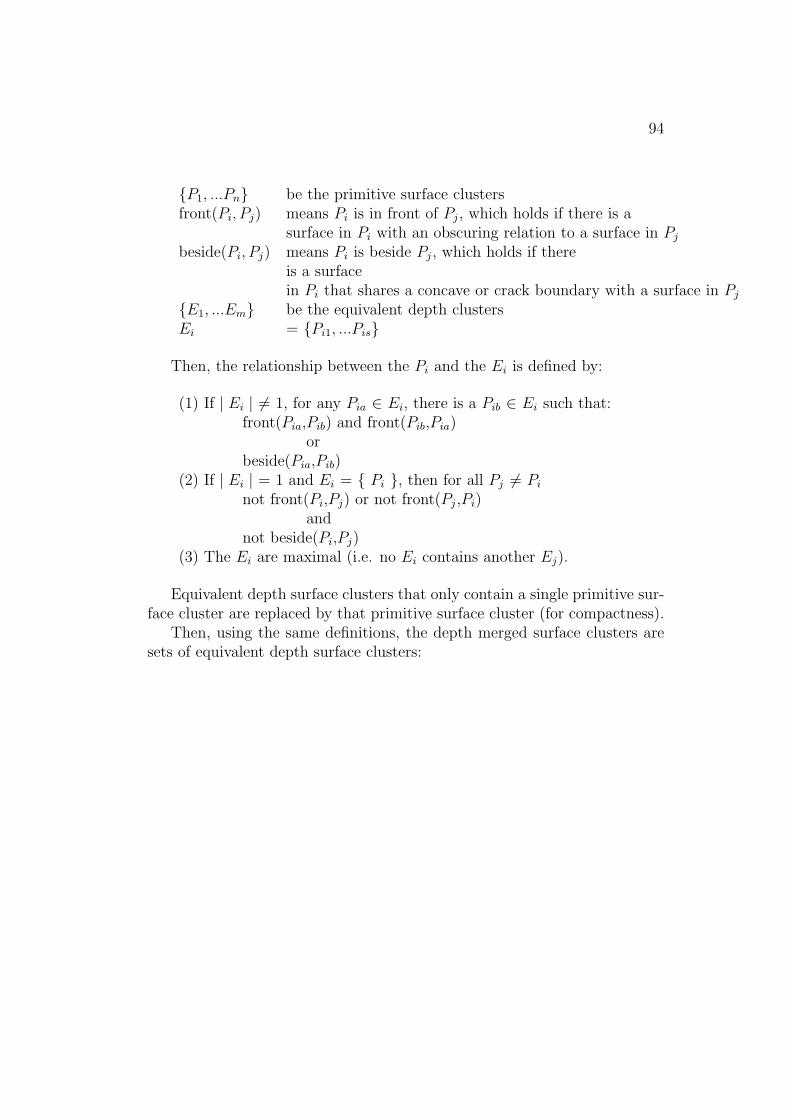
94

{P1, ...Pn} be the primitive surface clustersfront(Pi, Pj) means Pi is in front of Pj, which holds if there is a

surface in Pi with an obscuring relation to a surface in Pj

beside(Pi, Pj) means Pi is beside Pj, which holds if thereis a surfacein Pi that shares a concave or crack boundary with a surface in Pj

{E1, ...Em} be the equivalent depth clustersEi = {Pi1, ...Pis}

Then, the relationship between the Pi and the Ei is defined by:

(1) If | Ei | 6= 1, for any Pia ∈ Ei, there is a Pib ∈ Ei such that:front(Pia,Pib) and front(Pib,Pia)

orbeside(Pia,Pib)

(2) If | Ei | = 1 and Ei = { Pi }, then for all Pj 6= Pi

not front(Pi,Pj) or not front(Pj,Pi)and

not beside(Pi,Pj)(3) The Ei are maximal (i.e. no Ei contains another Ej).

Equivalent depth surface clusters that only contain a single primitive sur-face cluster are replaced by that primitive surface cluster (for compactness).

Then, using the same definitions, the depth merged surface clusters aresets of equivalent depth surface clusters:

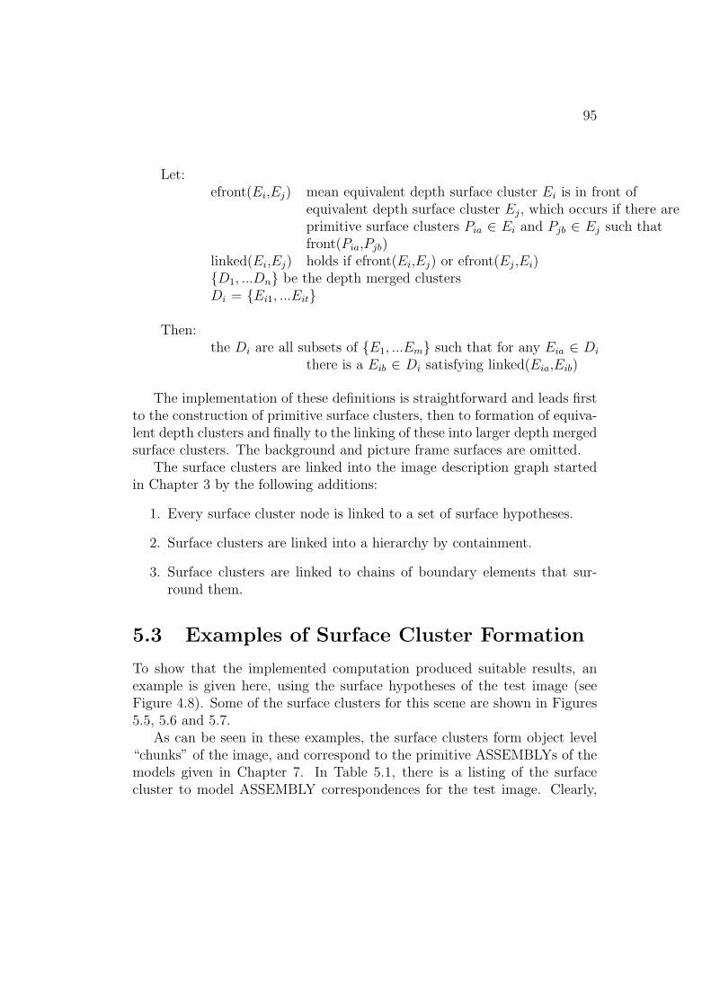
95

Let:efront(Ei,Ej) mean equivalent depth surface cluster Ei is in front of

equivalent depth surface cluster Ej, which occurs if there areprimitive surface clusters Pia ∈ Ei and Pjb ∈ Ej such thatfront(Pia,Pjb)

linked(Ei,Ej) holds if efront(Ei,Ej) or efront(Ej,Ei){D1, ...Dn} be the depth merged clustersDi = {Ei1, ...Eit}

Then:the Di are all subsets of {E1, ...Em} such that for any Eia ∈ Di

there is a Eib ∈ Di satisfying linked(Eia,Eib)

The implementation of these definitions is straightforward and leads firstto the construction of primitive surface clusters, then to formation of equiva-lent depth clusters and finally to the linking of these into larger depth mergedsurface clusters. The background and picture frame surfaces are omitted.

The surface clusters are linked into the image description graph startedin Chapter 3 by the following additions:

1. Every surface cluster node is linked to a set of surface hypotheses.

2. Surface clusters are linked into a hierarchy by containment.

3. Surface clusters are linked to chains of boundary elements that sur-round them.

5.3 Examples of Surface Cluster Formation

To show that the implemented computation produced suitable results, anexample is given here, using the surface hypotheses of the test image (seeFigure 4.8). Some of the surface clusters for this scene are shown in Figures5.5, 5.6 and 5.7.

As can be seen in these examples, the surface clusters form object level“chunks” of the image, and correspond to the primitive ASSEMBLYs of themodels given in Chapter 7. In Table 5.1, there is a listing of the surfacecluster to model ASSEMBLY correspondences for the test image. Clearly,

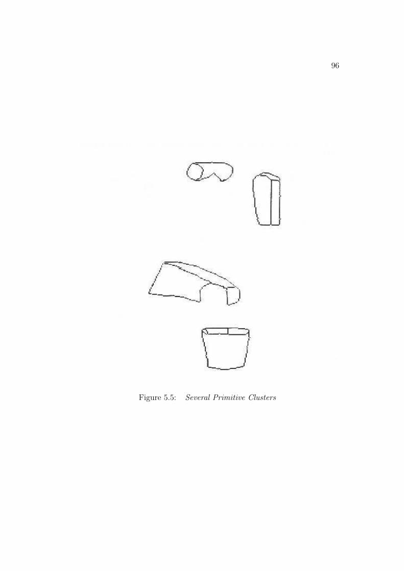
96

Figure 5.5: Several Primitive Clusters

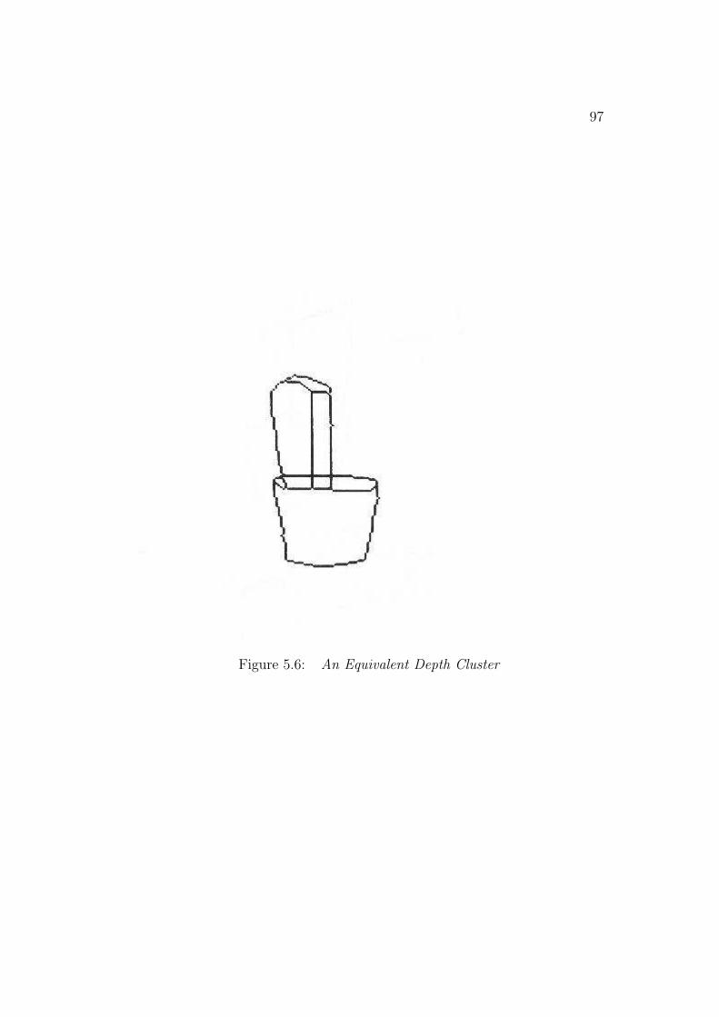
97

Figure 5.6: An Equivalent Depth Cluster

98

Figure 5.7: Several Depth Merged Clusters

99

the surface cluster formation process isolates the key features into what cor-responds to structurally based intuitive “objects”. Figure 5.8 showsthe surface clusters of Table 5.1 organized to make explicit their hierarchicalrelationships. Clusters designated by squares closely correspond to models.

For the example above, the primitive and equivalent depth surface clus-ters are appropriate. What seems to be a problem is the number of depthmerged surface clusters, which depend on combinatorial groupings of equiv-alent depth surface clusters. For the test scene, there are 9 primitive, 3equivalent depth and 6 depth merged surface clusters. Here, the number ofdepth merged surface clusters is not such a problem as the object also has astrong depth order, so 2 of the 6 correspond to ASSEMBLYs. In other testimages, shallower depth ordering causes more serious combinatorial grouping.Hence, an alternative process should be considered.

Though several surface clusters contained multiple ASSEMBLYs, thiscaused no recognition failures.

5.4 Relation to Other Work

In early two dimensional scene understanding work, Shirai [148] and Waltz[162] achieved a rough separation of objects from the background by assumingexternal boundaries of regions were the separator. Heuristics for addingisolated background regions, based on TEE matching, were suggested. Thesetechniques required that the background be shadow free, and that the objectsdid not contact the image boundary.

Both of these approaches concentrated on finding relevant objects byeliminating the irrelevant (i.e. the background). This was later seen to beunprofitable because relevance is usually determined at a higher level. Themethods were also incapable of decomposing the object grouping into smallerobject groups.

Guzman [81] started a sequence of work on surface segmentation usingimage topology. Starting from line drawings of scenes, he used heuristicsbased on boundary configurations at junctions to link together image re-gions to form complete bodies. Huffman [95] and Clowes [48] put Guzman’sheuristics into a more scientific form by isolating distinct bodies at connectedconcave and obscuring boundaries in two dimensional images.

Sugihara [155] proposed two heuristics for separating objects in an edgelabeled three dimensional light-stripe based range data image. The first sepa-

100

Table 5.1: Surface Cluster To Model Correspondences

SURFACE CLUSTER IMAGE

CLUSTER TYPE REGIONS MODEL

1 PRIMITIVE 20,21,30

2 PRIMITIVE 27

3 PRIMITIVE 16,26 robshldbd

4 PRIMITIVE 8 robbody

5 PRIMITIVE 29 robshldsobj

6 PRIMITIVE 33,34,35,36,37

7 PRIMITIVE 12,18,31 lowerarm

8 PRIMITIVE 9,28,38 trashcan

9 PRIMITIVE 17,19,22,25,32 upperarm

10 EQUIVALENT 20,21,27,30

11 EQUIVALENT 8,16,26,29 robshould + robbody

12 EQUIVALENT 9,12,18,28,31,38 lowerarm + trashcan

13 DEPTH 9,12,17,18,19,22, armasm + trashcan

25,28,31,32,38

14 DEPTH 8,16,17,19,22,

25,26,29,32

15 DEPTH 8,9,12,16,17, link + robot + trashcan

18,19,22,25,26,

28,29,31,32,38

16 DEPTH 8,16,20,21,26,

27,29,30

17 DEPTH 8,16,17,19,20,

21,22,25,26,27,

29,30,32

18 DEPTH 8,9,12,16,17,

18,19,20,21,22,

25,26,27,28,29,

30,31,32,38

101

6����

1����

HHHHj2��

��-

Includesunmodeled

objects

– – – – – – – – – – – – – – – – – – – – – – – – – – – – – –

Modeledstructure

3 HHHHj4 -

5 ����*

9 ����������:

7 -

8 ����*

10����

-

11 ��

����

HHHHj

12����

-

16����

-

14����

-���������

13 ��

��

��

17����

-

15 ���������

18����

Primitive EquivalentDepth

Depth Merged

- Model correspondence ����

- No model correspondence

Figure 5.8: Surface Cluster Hierarchy

102

rated objects where two obscuring and two obscured segments meet, depend-ing on a depth gap being detectable from either illumination or viewer effects.The second heuristic separated bodies along concave boundaries terminat-ing at special types of junctions (mainly involving two obscuring junctions).Other complexities arose because of the disparate illumination and sensorpositions.

Kak et al. [99] described segmentation from a labeled edge diagram thatconnects “cut”-type vertices with obscuring and concave edges, producing asegmentation similar to the primitive surface clusters.

The work described here extends the previous work for application to ob-jects with curved surfaces, some laminar surface groupings and hierarchicalobject structure. In particular, obscuring boundaries can become connect-ing (in certain circumstances) which allows the two laminar surfaces in thefolded leaf problem to become joined into a single surface cluster (Figure 5.3).Further, concave boundaries defining ambiguous depth relationships can beexploited to limit combinatorial explosion in the creation of larger surfaceclusters, which is necessary to provide the image context for structured ob-ject recognition.

Given the current input data, it is possible to directly infer from sur-face depth and orientation the type of surface discontinuity boundaries (i.e.obscuring, convex, concave). If the orientation data were missing, then topo-logical analysis like that from the two dimensional blocks world analysis (e.g.[95, 48, 162, 110, 161, 100, 162]) can sometimes uniquely deduce the three di-mensional boundary type. Labeling rules could also correct some data errors(e.g. [60]).

These projects also introduced the boundary labels of types obscuring(front surface, back surface) and shape discontinuity (convex, concave) thatare used for the reasoning described here. Also useful is the understandingof how boundary junctions relate to observer position and vertex structures(e.g. Thorpe and Shafer [160]).

5.5 Discussion

Surface clusters need not be perfect, as the goal of the process is to producea partitioning without a loss of information. They may be incomplete, aswhen an object is split up by a closer obscuring object, though the surfacehypothesizing may bridge the occlusion. They may also be over-aggregated

103

– from images where there is insufficient evidence to segregate two objects.These failures may reduce recognition performance (i.e. speed), but notits competence (i.e. success): incompletely merged surface clusters will bemerged in a larger context and insufficiently split surface clusters will justcause more searching during hypothesis construction.

The process of forming primitive surface clusters is particularly interestingbecause it is a local process (i.e. connectivity is determined by classificationsmade in the neighborhoods of vertices and single boundary segments) thatproduces a global organization of the image. This also holds for the for-mation of the equivalent depth surface clusters, but not the depth mergedclusters. Locality is important because (1) it is often required for efficientparallelization and (2) it is often the hallmark of a robust process.

A criticism concerns the combinatorial formation of the depth mergedsurface clusters. The general goal is to create hypotheses that correspondto the complete visible surface of an object and nothing more, necessitatingmerging surface clusters. Unfortunately, in the absence of context or objectknowledge, there is no information yet to determine whether a surface clusteris related to the surfaces behind. As an object may be associated with anytwo consecutive surfaces, it is likely that the merging process needs to bebased on either merging all surface clusters linked to the current one, orall possible combinations of consecutive depths. As each surface may bein front of more than one other surface, the latter alternative most likelyleads to a combinatorial explosion, whereas the former leads to enlargedsurface clusters. The combinatorial process, however, probably has betterfuture potential, provided some further merging constraints can be elucidatedand implemented. The use of equivalent depth clusters helped control theproblem, and as seen in Table 5.1, most of the surface clusters correspondto object features, an object was never split between surface clusters, andusually only one new model was appropriate for each new level of surfacecluster.

A general criticism about the surface cluster is that, as formulated here,it is too literal. A more suggestive process is needed for dealing with naturalscenes, where segmentation, adjacency and depth ordering are more ambigu-ous. The process should be supported by surface evidence, but should becapable of inductive generalization – as is needed to see a complete surfaceas covering the bough of a tree. The complexity of natural scenes is alsolikely to lead to combinatorial problems, because of the many objects over-lapping each other in dense scenes.

104

Final Comments

Surface clusters provide a good intermediate visual representation be-tween the segmented surface patches and the object hypotheses. In thechapters that follow, we will see how they are used to accumulate evidenceto select models and reduce the complexity of model matching.

Chapter 6

Description of ThreeDimensional Structures

The recognition of complex objects cannot be based on raw image data be-cause of its quantity and inappropriate level of representation. What reducesthe data to a manageable level is the process of feature description, thatproduces symbolic assertions such as “elongation(S,1.2)” or “shape(S,flat)”.

Besides providing the data compression that makes recognition computa-tionally tractable, description allows recognition processes to be more inde-pendent of the specific type of raw data, thus promoting generality. It mayalso simplify relationships; for example, an apple is approximately describedas a “reddish spheroid”.

One might ask: “What is the distinction between recognition and de-scription?”, because recognition also reduces sets of data to descriptions. Wewould be more inclined to say an image curve is “described as straight” thanis “recognized as a straight line”, whereas the reverse would apply to a per-son’s face. Thus, one criterion is simplicity – descriptions represent simple,consistent, generic phenomena. They are also more exact – “convex” allowsapproximate local reconstruction of a surface fragment, whereas “face” canhardly be more than representative.

If a description is dependent on a conjunction of properties, then it isprobably not suitable for use here (e.g. a “square” is a “curve” with equallength “side”s, each at “right angle”s). Hence, another criterion is generalapplicability, because “straight” is a useful description to consider for anyboundary, whereas “square” is not.

The descriptions presented here are simple unary and binary three di-

105

106

mensional properties of curves, surfaces and volumes such as curvature, areaor relative orientation. They are not reducible to subdescriptions (i.e. theyare not structured). Because we have three dimensional range data avail-able, it is possible to directly compute these properties, as contrasted to thedifficulties encountered when using two dimensional intensity data (thoughtwo dimensional data is also useful). The use of three dimensional data alsoallows richer and more accurate descriptions.

Pattern recognition techniques often estimate properties from two di-mensional projections of the structures, but cannot always do so correctly,because of the information lost in the projection process. To overcome this,some researchers have exploited constraints available from the real proper-ties of objects, such as the relationship between area and contour [38], fromassuming that curves are locally planar [154] or by assuming that a surfaceregion is a particular model patch [66].

Some of the properties considered below are viewpoint invariant. Theseproperties are important because they further the goal of viewpoint inde-pendent recognition. Moreover, the key invariant properties are local (e.g.curvature) as compared to global (e.g. area), because objects in three dimen-sional scenes are often partially obscured, which affects global properties.

Some Three Dimensional Structural Descrip-

tions

Here, three classes of structures acquire descriptions: boundaries, surfacesand surface clusters. The structures are interrelated and at times their de-scriptions depend on their relationships with other entities. We have iden-tified a variety of descriptions, some of which are listed below. Those num-bered have been implemented and their computations are described in thegiven section. Those that are viewpoint invariant are signaled by a “(V)”annotation.

• Boundary descriptions

– three dimensional boundary curvature (Section 6.1) (V)

– three dimensional boundary length (Section 6.2)

– three dimensional symmetry axis orientation

– parallel boundary orientation (Section 6.3) (V)

107

– relative boundary segment orientation (Section 6.4)

– relative boundary segment size

• Surface descriptions

– surface principal curvatures (Section 6.5) (V)

– surface curvature axis orientation (Section 6.5) (V)

– absolute surface area (Section 6.6)

– surface elongation (Section 6.7)

– relative surface orientation (Section 6.8) (V)

– relative surface size (Section 6.9)

– relative surface position

• Surface cluster descriptions

– surface cluster volume

– surface cluster elongation

– surface cluster elongation axis orientation

– surface cluster symmetry

– surface cluster relative volume

– surface cluster relative axis orientation

These three dimensional descriptions are reminiscent of the types of fea-tures used in traditional two dimensional pattern recognition approaches tocomputer vision (e.g. [14], pages 254-261). With these, one attempts tomeasure enough object properties to partition the feature space into distinctregions associated with single object classes. These techniques have beensuccessful for small model bases containing simple, distinct unobscured twodimensional objects, because the objects can then be partially and uniquelycharacterized using object-independent descriptions. Unfortunately, threedimensional scenes are more complicated because the feature values maychange as the object’s orientation changes, and because of occlusion.

The description processes discussed below extract simple global propertiesof curves and surfaces. The processes assume constant shape, but the actualfeatures are not always uniform, resulting in descriptions that are not always

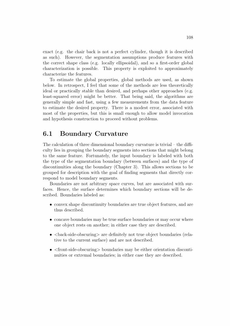
108

exact (e.g. the chair back is not a perfect cylinder, though it is describedas such). However, the segmentation assumptions produce features withthe correct shape class (e.g. locally ellipsoidal), and so a first-order globalcharacterization is possible. This property is exploited to approximatelycharacterize the features.

To estimate the global properties, global methods are used, as shownbelow. In retrospect, I feel that some of the methods are less theoreticallyideal or practically stable than desired, and perhaps other approaches (e.g.least-squared error) might be better. That being said, the algorithms aregenerally simple and fast, using a few measurements from the data featureto estimate the desired property. There is a modest error, associated withmost of the properties, but this is small enough to allow model invocationand hypothesis construction to proceed without problems.

6.1 Boundary Curvature

The calculation of three dimensional boundary curvature is trivial – the diffi-culty lies in grouping the boundary segments into sections that might belongto the same feature. Fortunately, the input boundary is labeled with boththe type of the segmentation boundary (between surfaces) and the type ofdiscontinuities along the boundary (Chapter 3). This allows sections to begrouped for description with the goal of finding segments that directly cor-respond to model boundary segments.

Boundaries are not arbitrary space curves, but are associated with sur-faces. Hence, the surface determines which boundary sections will be de-scribed. Boundaries labeled as:

• convex shape discontinuity boundaries are true object features, and arethus described.

• concave boundaries may be true surface boundaries or may occur whereone object rests on another; in either case they are described.

• <back-side-obscuring> are definitely not true object boundaries (rela-tive to the current surface) and are not described.

• <front-side-obscuring> boundaries may be either orientation disconti-nuities or extremal boundaries; in either case they are described.

109

The ring of boundary segments surrounding a surface is partitioned intodescribable sections by the following criteria:

1. If a segment has the label <back-side-obscuring>, then it is deleted.

2. If the point where two segments join is labeled as a boundary segmen-tation point, then split the ring at this point.

3. If two adjacent boundary segments have different labels, then split thering at their junction point.

Each set of connected boundary segments that remain after the splittingprocess is described.

For example, assume that the object in Figure 6.1 is sitting on a surface,that it is a box with an opening at surface 1, that boundary segment l belongsto the background and that the labelings are:

SEGMENT SURFACE LABELa 1 <front-side-obscuring>b 1 <back-side-obscuring>b 2 <front-side-obscuring>c 1 <back-side-obscuring>c 3 <front-side-obscuring>d 2,3 <convex>e 2 <front-side-obscuring>f 3 <front-side-obscuring>g 2 <concave>h 3 <concave>i 1 <front-side-obscuring>l ? any

110

Figure 6.1: Boundary Segment Grouping Example

VERTEX SEGMENTING JUNCTION?v1 yes (orientation discontinuity)v2 yes (orientation discontinuity)v3 yes (orientation discontinuity)

rest irrelevant

Then, the only describable boundary section for surface 1 is {a,i}. As band c are <back-side-obscuring>, they are not used. Segments a and i arenot separated by any criterion, so are treated as a single section. For surface2, each segment is isolated. Between b and d the label changes, as betweene and g. Between b and e there is a boundary segmentation point (placedbecause of an orientation discontinuity in the boundary), as between d andg. Surface 3 is similar to surface 2.

One goal of the boundary segmentation described in Chapter 3 was toproduce boundary sections with approximately uniform curvature character.Hence, assuming a boundary section is approximately circular, its curvaturecan be estimated as follows (referring to Figure 6.2):

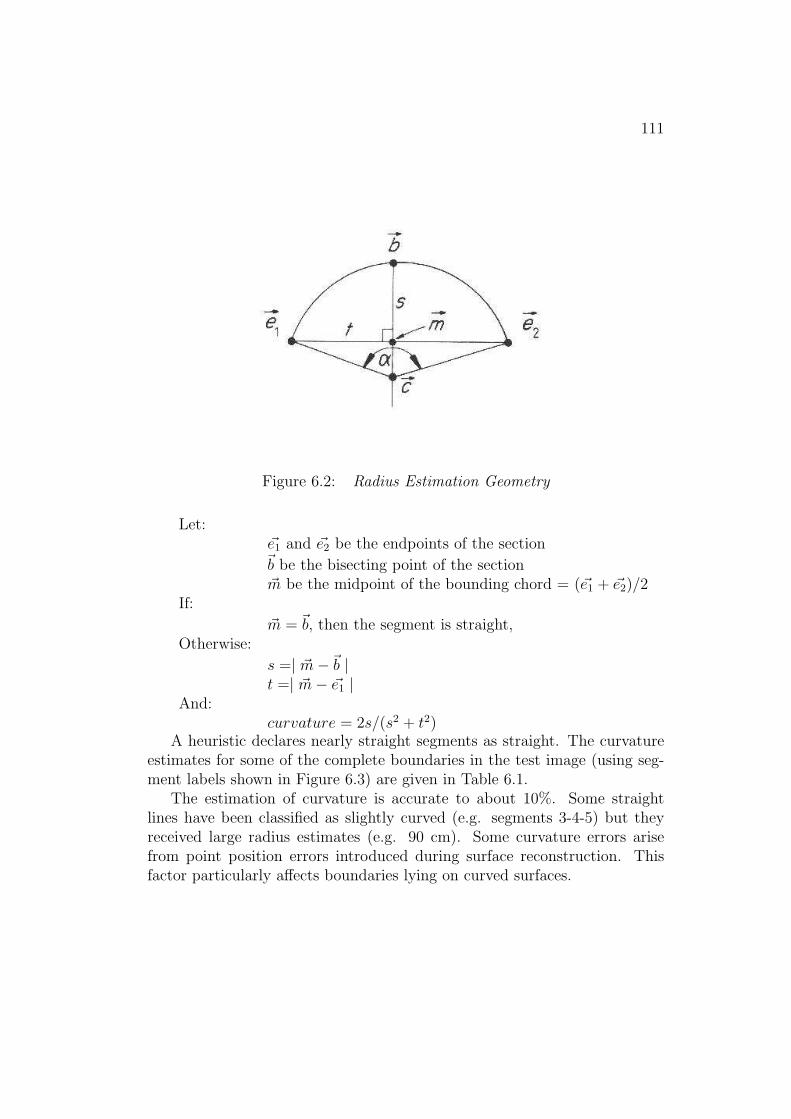
111

Figure 6.2: Radius Estimation Geometry

Let:~e1 and ~e2 be the endpoints of the section~b be the bisecting point of the section~m be the midpoint of the bounding chord = (~e1 + ~e2)/2

If:

~m = ~b, then the segment is straight,Otherwise:

s =| ~m −~b |t =| ~m − ~e1 |

And:curvature = 2s/(s2 + t2)

A heuristic declares nearly straight segments as straight. The curvatureestimates for some of the complete boundaries in the test image (using seg-ment labels shown in Figure 6.3) are given in Table 6.1.

The estimation of curvature is accurate to about 10%. Some straightlines have been classified as slightly curved (e.g. segments 3-4-5) but theyreceived large radius estimates (e.g. 90 cm). Some curvature errors arisefrom point position errors introduced during surface reconstruction. Thisfactor particularly affects boundaries lying on curved surfaces.

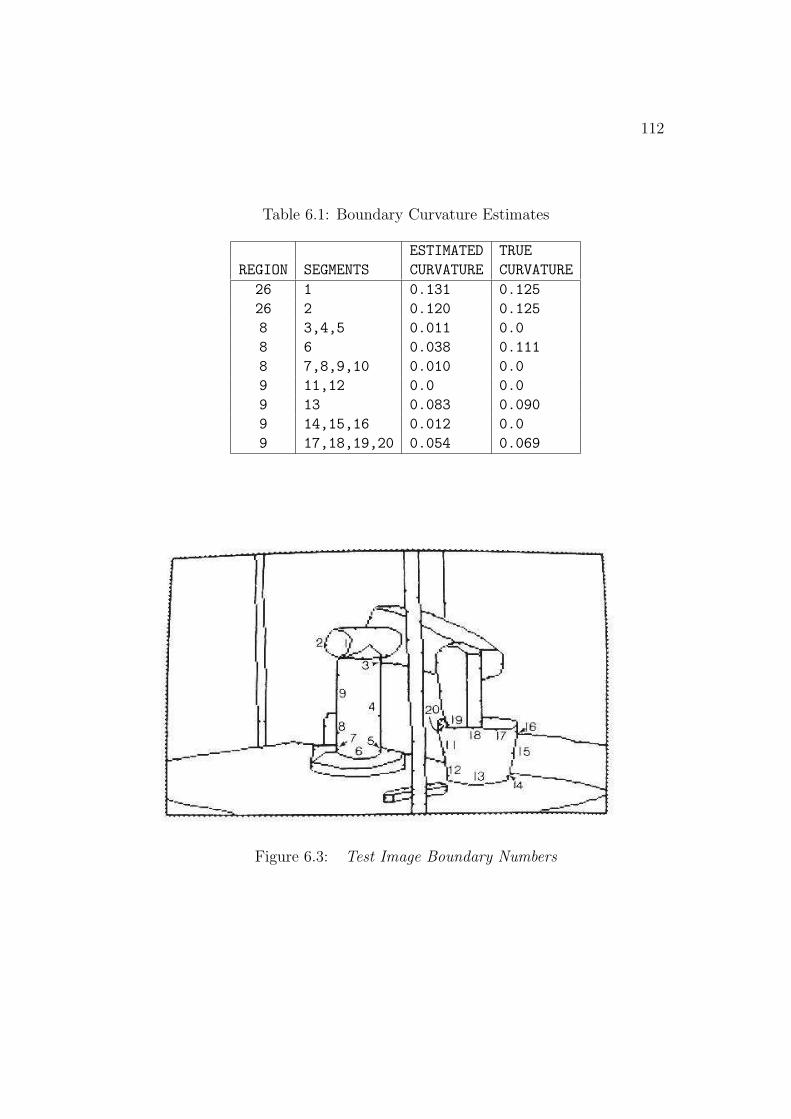
112

Table 6.1: Boundary Curvature Estimates

ESTIMATED TRUE

REGION SEGMENTS CURVATURE CURVATURE

26 1 0.131 0.125

26 2 0.120 0.125

8 3,4,5 0.011 0.0

8 6 0.038 0.111

8 7,8,9,10 0.010 0.0

9 11,12 0.0 0.0

9 13 0.083 0.090

9 14,15,16 0.012 0.0

9 17,18,19,20 0.054 0.069

Figure 6.3: Test Image Boundary Numbers

113

Table 6.2: Boundary Length Estimates

ESTIMATED TRUE

REGION SEGMENTS LENGTH LENGTH % ERROR

26 1 31.9 25.2 26

26 2 37.0 25.2 47

8 3,4,5 51.1 50.0 2

8 6 27.3 28.2 3

8 7,8,9,10 46.1 50.0 8

9 11,12 28.0 27.2 3

9 13 30.1 34.5 12

9 14,15,16 25.3 27.2 7

9 17,18,19,20 32.7 45.5 28

6.2 Boundary Length

Given the three dimensional data, the length of boundary segments can beestimated directly. If the segment is straight, then its length is just thedistance between its endpoints. Otherwise, given the groupings described inthe previous section, the calculated curvature and the geometric definitions,the length of a curved segment is given as follows (referring to Figure 6.2):

Let:

~u be the unit vector in the direction ~m −~b

~c = ~b + ~u/curvature be the center of the arc~ri be the unit vector from ~c to ~ei

Then:α = arccos(~r1 ◦ ~r2) is the angle subtended by the arc, andlength = α/curvature

The boundary length estimates for some of the complete boundaries inthe test image (segment labels from Figure 6.3) are shown in Table 6.2.

The average error for boundary length is about 20%, but there are largererrors. On the whole, the estimates are generally acceptable, though notaccurate. The poor estimates for segments 1 and 2 result from data errors.

114

6.3 Parallel Boundaries

A distinctive surface feature is the presence of parallel boundary sections.Hence, one potential description for surfaces is the number of groups of par-allel boundaries. In this context, parallel means in three dimensions, andrequires:

• vectors between endpoints to be parallel, and

• direction of arc curvature to be parallel.

The endpoint vector calculation is trivial given the three dimensionaldata. The direction vectors are the ~u defined in the previous section, so thesecond test is also easy. The results for the test image are given in Table 6.3.No errors occurred.

6.4 Relative Boundary Orientation

The angular relationships between sections of a segmented boundary are alsoa distinctive characteristic of the surface. The angle between the tangentsbefore and after the segmentation point is a potential measurement, but thiswould not discriminate between a short and a long arc smoothly joined toa straight segment (recalling that the boundary is segmented by orientationand curvature discontinuities). Further, estimation of the tangent angle isless reliable. Hence, the measurement chosen was the angle between thevectors through the segment endpoints, as illustrated in Figure 6.4. Partialocclusion of the boundary will affect this measurement for curved segments.However, if enough of the boundary is visible, the estimate will be close(assuming small curvatures).

Some of the join angles for complete object surfaces are reported in Ta-ble 6.4. The average angular estimation error is about 0.1 radian, so thisestimation process is acceptable.

6.5 Surface Curvature

By the surface shape segmentation assumptions (Chapter 3), each surfaceregion can be assumed to have constant curvature signs and approximately

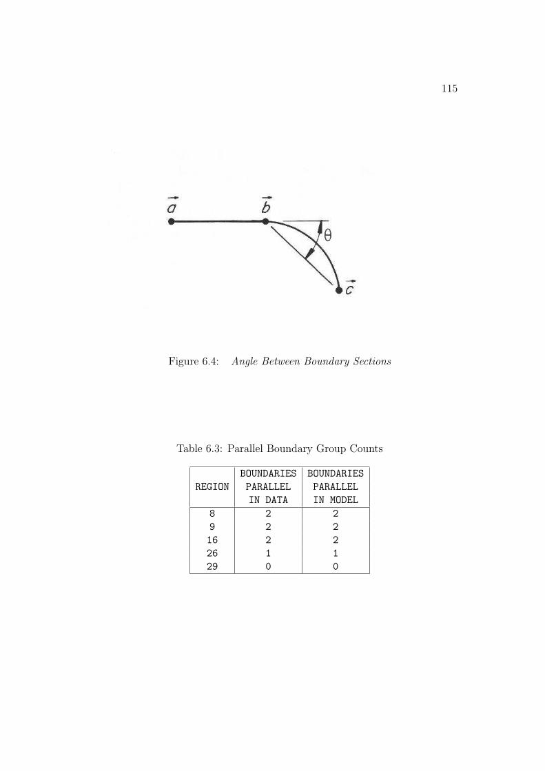
115

Figure 6.4: Angle Between Boundary Sections

Table 6.3: Parallel Boundary Group Counts

BOUNDARIES BOUNDARIES

REGION PARALLEL PARALLEL

IN DATA IN MODEL

8 2 2

9 2 2

16 2 2

26 1 1

29 0 0

116

Table 6.4: Boundary Join Angles

DATA MODEL

REGION SEGMENTS ANGLE ANGLE ERROR

26 1 - 2 3.14 3.14 0.0

26 2 - 1 3.14 3.14 0.0

8 3,4,5 - 6 1.40 1.57 0.17

8 6 - 7,8,9,10 1.79 1.57 0.22

9 11,12 - 13 1.73 1.70 0.03

9 13 - 14,15,16 1.64 1.70 0.06

9 14,15,16 - 1.45 1.44 0.01

17,18,19,20

9 17,18,19,20 - 1.45 1.44 0.01

11,12

constant curvature magnitude. Using the orientation information, the aver-age orientation change per image distance is estimated and this is then usedto estimate absolute curvature. This description separates surface regionsinto curvature classes, which provides a first level of characterization. Theabsolute magnitude of the curvature then provides a second description.

Following Stevens [153] and others, the two principal curvatures, κ1 andκ2, are used to characterize the local shape of the surface (along with thedirections of the curvatures). These are the maximum and minimum localcurvatures of the planar curves formed by intersecting a normal plane withthe surface. (The rotation angles at which these curvatures occur are orthog-onal – a property that will be used later.) The signs of the two curvaturescategorize the surfaces into six possible surface shape classes (Table 6.5).The curvature sign is arbitrary, and here convex surfaces are defined to havepositive curvature.

Turner [161] classified surfaces into five different classes (planar, spher-ical, conical, cylindrical and catenoidal) and made further distinctions onthe signs of the curvature, but here the cylindrical and conical categorieshave been merged because they are locally similar. Cernuschi-Frias, Bolleand Cooper [45] classified surface regions as planar, cylindrical or spherical,based on fitting a surface shading model for quadric surfaces to the observedimage intensities. Both of these techniques use intensity data, whereas di-

117

Table 6.5: Surface Shape Classes

κ1 < 0 κ1 = 0 κ1 > 0κ2 < 0 CONCAVE CONCAVE HYPERBOLOID

ELLIPSOID CYLINDER SURFACE

κ2 = 0 CONCAVE PLANE CONVEX

CYLINDER CYLINDER

κ2 > 0 HYPERBOLOID CONVEX CONVEX

SURFACE CYLINDER ELLIPSOID

rectly using the surface orientation data allows local computation of shape.Moreover, using only intensity patterns, the methods give a qualitative eval-uation of shape class, instead of absolute curvature estimates. More recently,Besl [24] used the mean and gaussian curvature signs (calculated from rangedata) to produce a similar taxonomy, only with greater differentiation of thehyperboloidal surfaces.

Brady et al. [40] investigated a more detailed surface understanding in-cluding locating lines of curvature of surfaces and shape discontinuities usingthree dimensional surface data. This work gives a more accurate metricalsurface description, but is not as concerned with the symbolic descriptionof surface segments. Agin and Binford [5] and Nevatia and Binford [121]segmented generalized cylinders from light-stripe based range data, derivingcylinder axes from stripe midpoints or depth discontinuities.

To estimate the curvature magnitude, we use the difference in the orien-tation of two surface normals spatially separated on the object surface. Theideal case of a cross-section perpendicular to the axis of a cylinder is shownin Figure 6.5. Two unit normals ~n1 and ~n2 are separated by a distance L onthe object surface. The angular difference θ between the two vectors is givenby the dot product:

θ = arccos( ~n1 ◦ ~n2)

Then, the curvature estimate at this cross-section orientation is:

κ = 2 ∗ sin(θ/2)/L

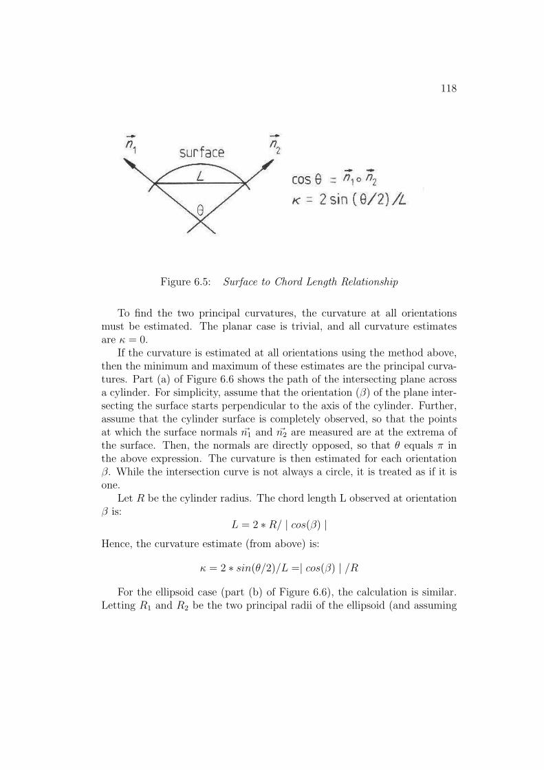
118

Figure 6.5: Surface to Chord Length Relationship

To find the two principal curvatures, the curvature at all orientationsmust be estimated. The planar case is trivial, and all curvature estimatesare κ = 0.

If the curvature is estimated at all orientations using the method above,then the minimum and maximum of these estimates are the principal curva-tures. Part (a) of Figure 6.6 shows the path of the intersecting plane acrossa cylinder. For simplicity, assume that the orientation (β) of the plane inter-secting the surface starts perpendicular to the axis of the cylinder. Further,assume that the cylinder surface is completely observed, so that the pointsat which the surface normals ~n1 and ~n2 are measured are at the extrema ofthe surface. Then, the normals are directly opposed, so that θ equals π inthe above expression. The curvature is then estimated for each orientationβ. While the intersection curve is not always a circle, it is treated as if it isone.

Let R be the cylinder radius. The chord length L observed at orientationβ is:

L = 2 ∗ R/ | cos(β) |Hence, the curvature estimate (from above) is:

κ = 2 ∗ sin(θ/2)/L =| cos(β) | /R

For the ellipsoid case (part (b) of Figure 6.6), the calculation is similar.Letting R1 and R2 be the two principal radii of the ellipsoid (and assuming

119

Figure 6.6: Cross-Section Length Relationships

that the third is large relative to these two) the length measured is approxi-mately:

L = 2 ∗ R1 ∗ R2/√

T

where:T = (R1 ∗ sin(β))2 + (R2 ∗ cos(β))2

Hence, the curvature estimate (from above) is:

κ = 2 ∗ sin(θ/2)/L =√

T/(R1 ∗ R2)

The special case of the cylinder can be derived from this by looking at thelimit as R2 approaches infinity.

This analysis gives the estimated curvature versus cross-section orienta-tion β. If β is not aligned with a principal curvature axis, then the cross-section has a shifted phase. In any case, the minimum and maximum valuesof these estimates are the principal curvatures. The maximum curvatureoccurs perpendicular to the major curvature axis (by definition) and theminimum curvature occurs at π/2 from the maximum. Figure 6.7 shows agraphical presentation of the estimated curvature versus β.

For simplicity, this analysis used the curvature estimated by picking op-posed surface normals at the extremes of the intersecting plane’s path. Realintersection trajectories will usually not reach the extrema of the surface andinstead we estimate the curvature with a shorter segment using the method

120

Figure 6.7: Ideal Estimated Curvature Versus Orientation

outlined at the beginning of this section. This produces different curvatureestimates for orientations not lying on a curvature axis. However, the majorand minor axis curvature estimates are still correct, and are still the max-imum and minimum curvatures estimated. Then, Euler’s relation for thelocal curvature estimated at orientations θ (not necessarily aligned with theprincipal curvatures) is exploited to find an estimate of the curvatures:

κ(β) = κ1 ∗ cos2(β) + κ2 ∗ sin2(β) = κ2 + (κ1 − κ2) ∗ cos2(β)

One might ask why the global separated normal vector approach to cur-vature estimation was used, rather than using derivatives of local orientationestimates, or the fundamental forms? The basis for this decision is that wewanted to experiment with using the larger separation to reduce the error inthe orientation difference θ when dealing with noisy data. This benefit hasto be contrasted with the problem of the curvature changing over distance.But, as the changes should be small by the segmentation assumption, theestimation should still be reasonably accurate. Other possibilities that werenot tried were least-squared error fitting of a surface patch and fitting a curveto the set of normals obtained along the cross-section at each orientation β.

We now determine the sign of the curvature. As Figure 6.8 shows, theangle between corresponding surface normals on similar convex and concavesurfaces is the same. The two cases can be distinguished because for convexsurfaces the surface normals point away from the center of curvature, whereas

121

Figure 6.8: Convex and Concave Surface Similarities

for the concave case the surface normals point towards it.Given the above geometric analysis, the implemented surface curvature

computation is:

1. Let ~P be a nominal point in the surface image region.

2. Generate the curvature estimate versus β function as outlined above,for cross-sections through ~P :

(a) find cross-section length L

(b) find surface orientation angle difference θ

(c) estimate curvature magnitude | κ |

3. Fit cos2(α) to the curvature versus β function to smooth estimates anddetermine the phase angle.

4. Extract maximum and minimum curvature magnitudes.

5. At maximum and minimum curvature orientations, check direction ofsurface normal relative to surface.

122

Figure 6.9: Curvature Axis Orientation Estimation (Find Axis Plane)

(a) if towards the center, then κ < 0

(b) if away from the center, then κ > 0

The estimation of the major axis orientation for the surface region is noweasy. (The major axis is that about which the greatest curvature occurs.)The plane case can be ignored, as it has no curvature. Figures 6.9 and 6.10illustrate the geometry for the axis orientation estimation process.

We calculate the axis direction by calculating the direction of a parallelline ~a through the nominal point ~P . We start by finding a plane X that thisline lies in (see Figure 6.9). Plane X contains the viewer and the nominal

point ~P . Hence, the vector ~v2 from the viewer to the nominal point lies in theplane. Further, we assume that line ~a projects onto the image plane at theimage orientation θ at which the minimum curvature is estimated. Hence,the vector ~v1 = (cos(θ), sin(θ), 0) also lies in plane X. As the two vectors aredistinct (~v1 is seen as a line, whereas ~v2 is seen as a point), the normal ~n1 toplane X is:

~n1 = ~v1 × ~v2

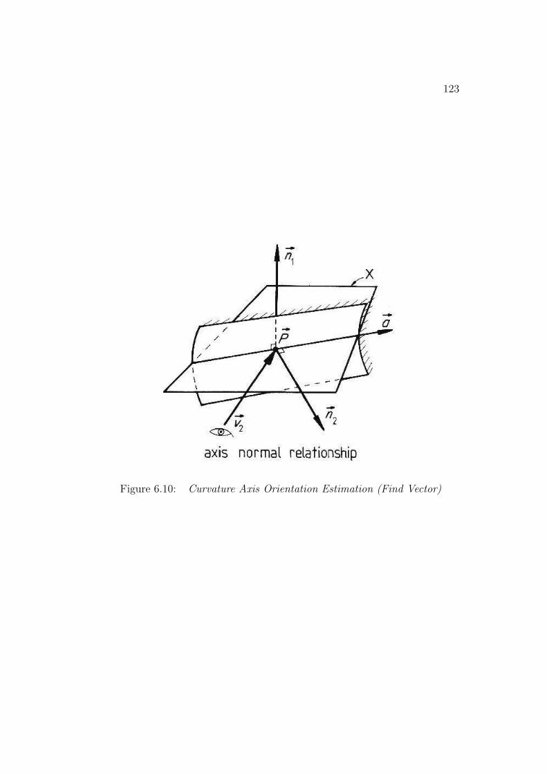
123

Figure 6.10: Curvature Axis Orientation Estimation (Find Vector)

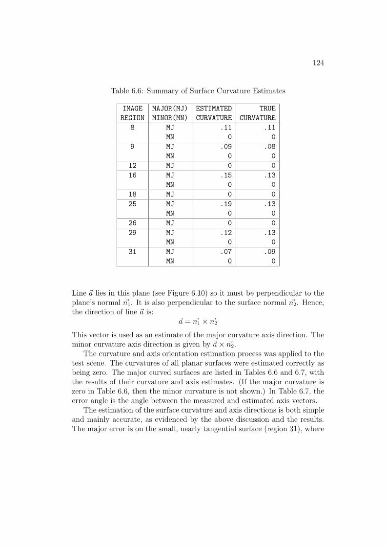
124

Table 6.6: Summary of Surface Curvature Estimates

IMAGE MAJOR(MJ) ESTIMATED TRUE

REGION MINOR(MN) CURVATURE CURVATURE

8 MJ .11 .11

MN 0 0

9 MJ .09 .08

MN 0 0

12 MJ 0 0

16 MJ .15 .13

MN 0 0

18 MJ 0 0

25 MJ .19 .13

MN 0 0

26 MJ 0 0

29 MJ .12 .13

MN 0 0

31 MJ .07 .09

MN 0 0

Line ~a lies in this plane (see Figure 6.10) so it must be perpendicular to theplane’s normal ~n1. It is also perpendicular to the surface normal ~n2. Hence,the direction of line ~a is:

~a = ~n1 × ~n2

This vector is used as an estimate of the major curvature axis direction. Theminor curvature axis direction is given by ~a × ~n2.

The curvature and axis orientation estimation process was applied to thetest scene. The curvatures of all planar surfaces were estimated correctly asbeing zero. The major curved surfaces are listed in Tables 6.6 and 6.7, withthe results of their curvature and axis estimates. (If the major curvature iszero in Table 6.6, then the minor curvature is not shown.) In Table 6.7, theerror angle is the angle between the measured and estimated axis vectors.

The estimation of the surface curvature and axis directions is both simpleand mainly accurate, as evidenced by the above discussion and the results.The major error is on the small, nearly tangential surface (region 31), where

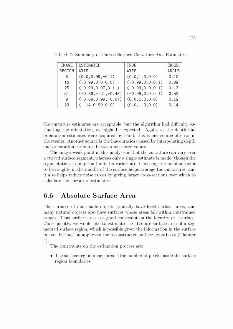
125

Table 6.7: Summary of Curved Surface Curvature Axis Estimates

IMAGE ESTIMATED TRUE ERROR

REGION AXIS AXIS ANGLE

8 (0.0,0.99,-0.1) (0.0,1.0,0.0) 0.10

16 (-0.99,0.0,0.0) (-0.99,0.0,0.1) 0.09

25 (-0.99,0.07,0.11) (-0.99,0.0,0.1) 0.13

31 (-0.86,-.21,-0.46) (-0.99,0.0,0.1) 0.53

9 (-0.09,0.99,-0.07) (0.0,1.0,0.0) 0.12

29 (-.14,0.99,0.0) (0.0,1.0,0.0) 0.14

the curvature estimates are acceptable, but the algorithm had difficulty es-timating the orientation, as might be expected. Again, as the depth andorientation estimates were acquired by hand, this is one source of error inthe results. Another source is the inaccuracies caused by interpolating depthand orientation estimates between measured values.

The major weak point in this analysis is that the curvature can vary overa curved surface segment, whereas only a single estimate is made (though thesegmentation assumption limits its variation). Choosing the nominal pointto lie roughly in the middle of the surface helps average the curvatures, andit also helps reduce noise errors by giving larger cross-sections over which tocalculate the curvature estimates.

6.6 Absolute Surface Area

The surfaces of man-made objects typically have fixed surface areas, andmany natural objects also have surfaces whose areas fall within constrainedranges. Thus surface area is a good constraint on the identity of a surface.Consequently, we would like to estimate the absolute surface area of a seg-mented surface region, which is possible given the information in the surfaceimage. Estimation applies to the reconstructed surface hypotheses (Chapter4).

The constraints on the estimation process are:

• The surface region image area is the number of pixels inside the surfaceregion boundaries.

126

• The image area is related to the surface area of a fronto-parallel planarsurface at a given depth by the camera parameters.

• The area of a fronto-parallel planar surface is related to the area of anoriented planar surface by its surface orientation.

• The area of a curved surface is related to the area of the equivalentprojected planar surface by the magnitude of its curvature.

The effects of surface curvature are approximately overcome using twocorrection factors for the principal curvatures, which are calculated in thefollowing manner. In Figure 6.11 part (a), the case of a single dimension isconsidered. A curved segment of curvature C subtends an angle θ . Hence, ithas length θ/C. This appears in the image as a straight segment of length L.So, the curvature correction factor relating the length of a curved segmentto the equivalent chord is:

F = θ/(L ∗ C)

where the angle θ is given by:

θ = 2 ∗ arcsin(L ∗ C/2)

Hence, the complete curvature correction factor is (if C > 0):

F = 2 ∗ arcsin(L ∗ C/2)/(L ∗ C)

elseF = 1

Now, referring to Figure 6.11 part (b), the absolute surface area is esti-mated as follows:

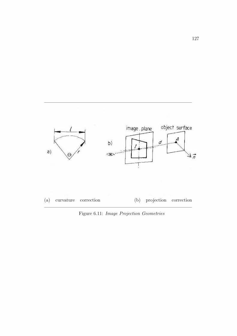
127

(a) curvature correction (b) projection correction

Figure 6.11: Image Projection Geometries

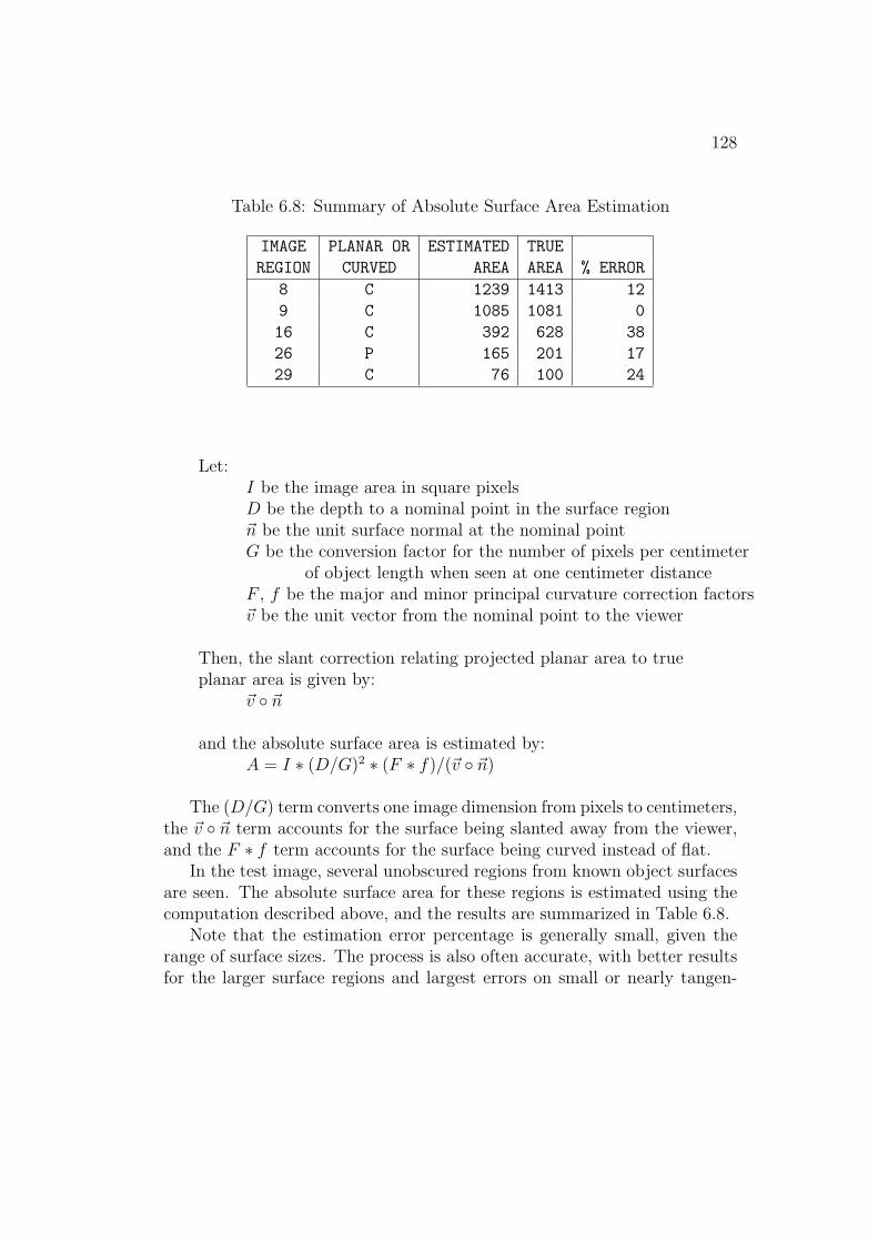
128

Table 6.8: Summary of Absolute Surface Area Estimation

IMAGE PLANAR OR ESTIMATED TRUE

REGION CURVED AREA AREA % ERROR

8 C 1239 1413 12

9 C 1085 1081 0

16 C 392 628 38

26 P 165 201 17

29 C 76 100 24

Let:I be the image area in square pixelsD be the depth to a nominal point in the surface region~n be the unit surface normal at the nominal pointG be the conversion factor for the number of pixels per centimeter

of object length when seen at one centimeter distanceF , f be the major and minor principal curvature correction factors~v be the unit vector from the nominal point to the viewer

Then, the slant correction relating projected planar area to trueplanar area is given by:

~v ◦ ~n

and the absolute surface area is estimated by:A = I ∗ (D/G)2 ∗ (F ∗ f)/(~v ◦ ~n)

The (D/G) term converts one image dimension from pixels to centimeters,the ~v ◦ ~n term accounts for the surface being slanted away from the viewer,and the F ∗ f term accounts for the surface being curved instead of flat.

In the test image, several unobscured regions from known object surfacesare seen. The absolute surface area for these regions is estimated using thecomputation described above, and the results are summarized in Table 6.8.

Note that the estimation error percentage is generally small, given therange of surface sizes. The process is also often accurate, with better resultsfor the larger surface regions and largest errors on small or nearly tangen-

129

tial surfaces. The key sources of error are pixel spatial quantization, whichparticularly affects small regions, and inaccurate shape data estimation.

From the above discussion, the estimation process is obviously trivial,given the surface image as input. Since the goal of the process is only toacquire a rough estimate, the implemented approach is adequate.

6.7 Surface Elongation

The elongation of a surface region is also a distinguishing characteristic.This has been a traditional pattern recognition measurement applied to twodimensional regions, but a three dimensional version can also be obtained.

For a planar surface, elongation is the ratio of the longest to the shortestdimension of a planar rectangular box circumscribing the surface, which issimilar to the two dimensional definition. The definition can be adaptedto curved surfaces by using the maximum and minimum arc lengths of theintersection of the surface and a plane normal to the surface. The arc lengthshould be calculated for all intersections of the surface, but this is time-consuming. Instead, only the cross-section widths about a central point areused.

The four factors involved in the estimation of the surface’s dimensionsare: the image region’s dimensions, the surface slant relative to the viewer,the curvature of the surface, and the distance from the viewer. It is possibleto approximate the elongation after separating the effects of these factors.

Figure 6.12 part (a) shows a sketch of the viewing relationship at onecross-section through the surface. By the discussion in the previous section,the cross-section length S is approximately related to the chord length L as:

S = L ∗ θ/(2 ∗ sin(θ/2))

Then, if the cross-section is slanted away from the viewer by an angle α ,the observed slanted length L′ is approximately related to the chord lengthL (assuming the viewing distance is large) by:

L′ = L ∗ cos(α)

Finally, the observed image length I for the surface at depth D with conver-sion factor G (as in Section 6.6) is:

I = L′ ∗ (G/D)

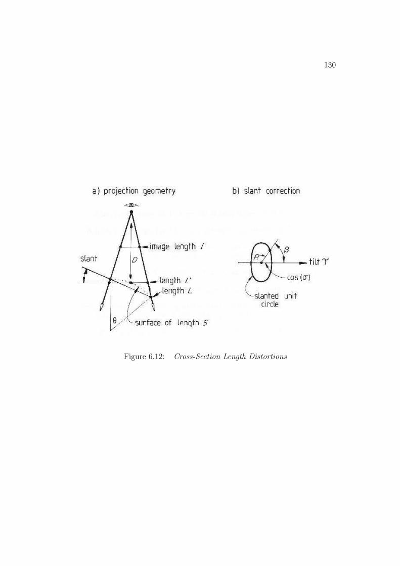
130

Figure 6.12: Cross-Section Length Distortions

131

This analysis is then modified for observed slant compression at anglesother than the tilt angle. Figure 6.12 part (b) shows the geometry used forthe following analysis. This figure shows a unit circle compressed by a slantangle σ in the direction τ and orthographically projected onto the imageplane. Elementary trigonometry and algebra show that the observed lengthR at the angle β is:

R = 1/√

1 + (tan(σ) ∗ cos(β))2

The computation of the elongation value is then:

Let:~N be a nominal point in the center of the surface image region

w(α) be the image cross-section width at image angle α about ~Nθ(α) be the change in surface orientation across

the cross-section at image angle α

(P,Q,−T ) be the unit surface normal at ~N

D be the distance from the viewer to ~NG be the conversion factor for the number of pixels per centimeter

of object length when seen at one centimeter distance

~v be the unit vector pointing to the viewer from the point ~N

Then, the tilt angle is:

τ = arctan(Q/P )

the relative slant direction β is:

β = α − τ

the slant angle σ is:σ = arccos(~v ◦ (P,Q,−T ))

the slant correction factor is:

M =√

1 + (tan(σ) ∗ cos(β))2

the projected chord length L’ is:

L′(α) = w(α) ∗ (D/G)

132

Table 6.9: Summary of Estimated Elongations

IMAGE PLANAR OR ESTIMATED TRUE

REGION CURVED ELONGATION ELONGATION

8 C 3.3 2.0

9 C 1.8 1.7

16 C 2.9 1.5

26 P 1.4 1.0

29 C 3.6 3.1

the unprojected chord length L is:

L(α) = L′(α) ∗ M

and the estimated three dimensional cross-section is:

cross(α) = L(α) ∗ θ(α)/(2 ∗ sin(θ(α)/2))

Finally, the elongation is:

E = maxα(cross(α))/minα(cross(α))

The elongations for all unobscured image regions that directly correspondto model SURFACEs are listed in Table 6.9.

These results show that the estimation process gives approximate resultswhen applied to unobscured regions. In part, small regions should be moreaffected because single pixel errors are significant, but this is not always thecase.

A weakness of the process is that it only estimates the dimensions basedon reconstructions about a single point, which produces lower bounds for themaximum and upper bounds for the minimum cross-sections. This shouldresult in an estimate that is lower than the true elongation. However, thekey source of error is the small size of the regions coupled with image quan-tization. Other sources of error are the hand measured surface data, surfaceinterpolation and the curvature correction process assuming uniform curva-ture along the cross-section path. However, the approximations were feltto be justifiable on practical grounds and the above results show that theapproach is acceptable.

133

Figure 6.13: Two Adjacent Surfaces

6.8 Relative Surface Orientation

Given surface orientation and some elementary geometry, it is possible toestimate the angle at which two surfaces meet (defined as the angle that thesolid portion of the junction subsumes). This description is useful for tworeasons: (1) extra information is always useful for recognition and (2) themeasurement is dependent on the surface’s relationship with its neighbors,whereas many other descriptions relate only to the structure in isolation.Hence, context can enhance the likelihood of identification.

This description is only applied to surfaces that are adjacent across ashape boundary and so emphasizes group identification. (Surfaces across anobscuring boundary may not be related.)

The factors involved in the description’s calculation are the orientation ofthe surfaces, the shared boundary between the surfaces and the direction tothe viewer. As the boundary is visible, the viewer must be in the unoccupiedspace sector between the two surfaces.

Because surfaces can be curved, the angle between them may not beconstant along the boundary; however, it is assumed that this angle will notvary significantly without the introduction of other shape segmentations.Consequently, the calculation obtained at a nominal point is taken to berepresentative.

Figure 6.13 shows two surfaces meeting at a boundary. Somewhere alongthis boundary a nominal point ~P is chosen and also shown is the vector ofthe boundary direction at that point ( ~B). Through this point a cross-section

134

Figure 6.14: Surface Normals and the Two Surface Cases

plane is placed, such that the normals (~n) for the two surfaces lie in theplane. Figure 6.14 shows the two cases for this cross-section.

The essential information that determines the surface angle is the angle atwhich the two normals meet. However, it must also be determined whetherthe surface junction is convex or concave, which is the difficult portion ofthe computation. The details of the solution are seen in Figure 6.14. Letvectors ~S1 and ~S2 be tangential to the respective surfaces in the cross-sectionplane. By definition, the vector ~B is normal to the plane in which the ~ni

and ~Si vectors lie. Hence, each individual ~Si vector is normal to both thecorresponding ~ni vector and the ~B vector, and can be calculated by a crossproduct.

These ~Si vectors may face the wrong direction (e.g. away from the sur-

face). To obtain the correct direction, a track is made from the point ~P in

the direction of both ~Si and −~Si. One of these should immediately enter thesurface region, and this is assumed to be the correct ~Si vector.

Because the boundary must be visible, the angle between the vector ~vfrom the nominal point to the viewer and a surface vector ~Si must be lessthan π. Hence, the angle between these vectors is guaranteed to representopen space. Then, the angle between the two surfaces is 2π minus these twoopen spaces. This computation is summarized below:

135

Table 6.10: Summary of Relative Surface Orientation

IMAGE ESTIMATED TRUE

REGIONS ANGLE ANGLE ERROR NOTE

16,26 1.47 1.57 0.10

16,29 2.96 3.14 0.18

12,18 1.53 1.57 0.04

12,31 1.60 1.57 0.03

18,31 2.03 2.14 0.11

17,25 2.09 3.14 1.05 *

17,22 1.56 1.57 0.01

* – large error across a curvature discontinuity

Let:~P be a nominal point on the boundary between the two surfaces

~n1, ~n2 be the two surface normal vectors at ~P~v be the vector from the nominal point to the viewer

Then, the boundary vector ~B is:~B = ~n1 × ~n2

and the surface vectors ~Si are:~Si = ~B × ~ni

which are then adjusted for direction, as described above.Given this, the surface angle is:

θ = 2π− | arccos(~v ◦ ~S1) | − | arccos(~v ◦ ~S2) |

The true and estimated surface angles for the modeled objects are sum-marized in Table 6.10. Further, only rigid angles between surfaces in thesame primitive surface clusters are reported (these being the only evidenceused).

The estimation procedure is accurate for orientation discontinuities. Themajor source of errors for this process is the measurement of the surface ori-entation vectors by hand, and interpolating their value to the nominal point.

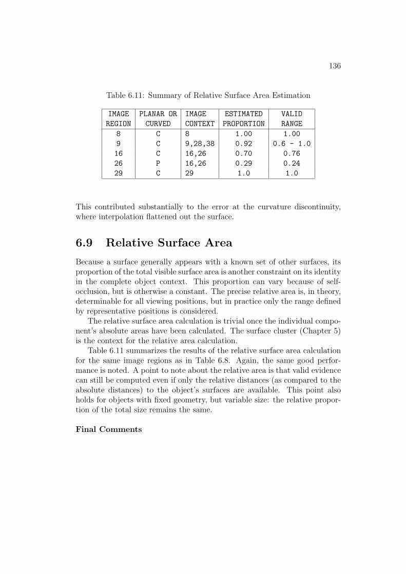
136

Table 6.11: Summary of Relative Surface Area Estimation

IMAGE PLANAR OR IMAGE ESTIMATED VALID

REGION CURVED CONTEXT PROPORTION RANGE

8 C 8 1.00 1.00

9 C 9,28,38 0.92 0.6 - 1.0

16 C 16,26 0.70 0.76

26 P 16,26 0.29 0.24

29 C 29 1.0 1.0

This contributed substantially to the error at the curvature discontinuity,where interpolation flattened out the surface.

6.9 Relative Surface Area

Because a surface generally appears with a known set of other surfaces, itsproportion of the total visible surface area is another constraint on its identityin the complete object context. This proportion can vary because of self-occlusion, but is otherwise a constant. The precise relative area is, in theory,determinable for all viewing positions, but in practice only the range definedby representative positions is considered.

The relative surface area calculation is trivial once the individual compo-nent’s absolute areas have been calculated. The surface cluster (Chapter 5)is the context for the relative area calculation.

Table 6.11 summarizes the results of the relative surface area calculationfor the same image regions as in Table 6.8. Again, the same good perfor-mance is noted. A point to note about the relative area is that valid evidencecan still be computed even if only the relative distances (as compared to theabsolute distances) to the object’s surfaces are available. This point alsoholds for objects with fixed geometry, but variable size: the relative propor-tion of the total size remains the same.

Final Comments

137

This chapter showed that surface data allowed a variety of general identity-independent three dimensional properties. These were directly computablefor curves, surfaces and surface clusters, using simple computations that esti-mated the properties acceptably. More work is needed to extend the numberof properties, improve the algorithms and determine their stability over awider range of objects.

Chapter 7

Object Representation

To recognize objects, one must have an internal representation of an objectsuitable for matching its features to image descriptions. There are severalapproaches to modeling, and this research uses a surface-based object repre-sentation distinguished by its use of shape segmentable surfaces organized ina subcomponent hierarchy. This approach provides the information neededto efficiently recognize and locate complicated articulated structures (like arobot) when using the input data described in Chapter 3.

This chapter also briefly describes the SMS modeling approach [70], whosedevelopment was based on experience with the IMAGINE I system.

7.1 The Geometric Model

The model is what the system knows about an object. Paraphrasing Bin-ford [29]: a capable vision system should know about object shape, and howshape affects appearance, rather than what types of images an object is likelyto produce. Geometric models explicitly represent the shape and structureof an object, and from these, one can (1) deduce what features will be seenfrom any particular viewpoint and where they are expected to be and (2)determine under what circumstances a particular image relationship is con-sistent with the model. Both of these conditions promote efficient featureselection, matching and verification. Hence, this approach is intrinsicallymore powerful than the property method, but possibly at the expense ofcomplexity and substantial computational machinery. However, a practicalvision system may also incorporate redundant viewer-centered descriptions,

138

139

to improve efficiency.The geometric body model used here introduces a uniform level of descrip-

tion suitable for a large class of objects (especially man-made). It specifiesthe key primitive elements of an object representation, and how they arepositioned relative to the whole object.

Some Requirements on the ModelThe models should emphasize the relevant aspects of objects. As this re-

search is concerned with model shape and structure, rather than reflectance,these are: surface shape, intersurface relationships (e.g. adjacency and rel-ative orientation), surface-object relationships and subcomponent-object re-lationships. To recognize the objects in the test scene, the geometric modelswill have to:

• make surface information explicit – to easily match image surface data,

• have three dimensional, transformable object-centered representations– because objects can take arbitrary, unexpected spatial locations andorientations,

• have geometric subcomponent relationships – because of the structur-ing of the surface clusters and the physical constraints on their place-ment,

• represent solid and laminar objects – to handle the variety in the sceneand

• have attachments with degrees-of-freedom – for recognizing articulatedobjects (e.g. the robot).

These are general requirements; more specific requirements for geometricinformation are discussed below.

As model invocation (Chapter 8) is based on both image property evi-dence and component associations, it additionally needs:

• size, shape and curvature parameters of individual surfaces and bound-ary segments,

• non-structural object relations, such as subtype or subclass,

• adjacency of surfaces and their relative orientation and

140

• typical configurations of visible components.

Hypothesis construction and verification (Chapters 9 and 10) instantiateand validate invoked models by pairing image data or previously recognizedobjects with model components. To build the hypotheses, the matcher willhave to search the image and its results database for evidence. Verificationascertains the soundness of the instantiated models by ensuring that thesubstructures have the correct geometric relationship with each other andthe model as a whole, and that the assembled object forms a valid andcompact solid. Together, the two processes require:

• the type of substructures needed and

• the geometric relationships between the substructures and the object.

Model PrimitivesModel surfaces and boundaries are usually segmented according to the

same criteria discussed in Chapter 3 for image data (essentially shape discon-tinuities). Hence, the same primitives are also used for the models to reducethe conceptual distance to the data primitives, and thus simplify matching.The primitive element of the model is the SURFACE, a one-sided boundedtwo dimensional (but not necessarily flat) structure defined in a three dimen-sional local reference frame. A SURFACE has two primary characteristics –surface shape, and extent.

Surface shape is defined by its surface class, the curvature axes andthe curvature values. The surface classes are planar, cylindrical and ellip-soidal/hyperboloidal. The curvature values can be positive or negative, rep-resenting convex or concave principal curvatures about the curvature axes.The minor curvature axis (if any) is orthogonal to both the surface normaland the major curvature axis. (This is always locally true and it also holdsglobally for the surface primitives used here.) These model patches are ex-actly the same as the data patches shown in Figure 3.10, except for wherethe data patches are not fully seen because of occlusion or inappropriateviewpoint. While many other surface shape representations are used, thisone was chosen because:

• surface shape is characterized by two parameters only (the principalcurvatures), and it is felt that these can be successfully estimated fromimage data (e.g. [40]). Further, it is felt that it will be difficult toreliably estimate more detailed information.

141

• Even if the precise curvature values are not extractable, shape classshould be, using a variety of shape cues (e.g. specularity, shadows,shading, etc.).

The definition of surface shapes is straightforward for the planar andcylindrical (and conical) patches. Each SURFACE is defined relative to alocal coordinate system. The plane is implicitly defined to pass through(0, 0, 0) with a normal of (0, 0,−1) and has infinite extent. A cylinder is con-vex or concave according to the sign of its curvature, has a defined curvaturemagnitude and axis of curvature, and has infinite extent.

Surfaces that curve in two directions are not well represented here. Theproblem is that on these surfaces, curvature varies everywhere (except for ona perfect sphere), whereas we would like to characterize the surface simplyand globally. Given the segmentation criteria, one feature that does remainconstant is the sign of the principal curvatures. To make the characteri-zation more useful, we also include the magnitudes and three dimensionaldirections of the curvatures at a nominal central point. While this is just anapproximation, it is useful for model matching.

When it is necessary to draw or predict instances of these SURFACEs,the model used is (r1 = radius1, r2 = radius2):

sign(r1) ∗(x′)2

r21

+ sign(r2)(y′)2

r22

+(z)2

r2z

= 1

where rz = 50 (an arbitrary choice) and (x′, y′) are in a coordinate systemthat places x′ along the major curvature axis.

Surfaces with twist are neither modeled nor analyzed.All SURFACEs are presumed to bound solids; laminar surfaces are formed

by joining two model SURFACEs back to back. Hence, the normal directionalso specifies the outside surface direction.

The extent of a SURFACE is defined by a three dimensional polycurveboundary. The surface patch lies inside the boundary, when it is projectedonto the infinite surface. These patches are intended to be only approximateas: (1) it is hard to characterize when one surface stops and another startson curved surfaces, and (2) surface extraction and description processes donot reliably extract patch boundaries except near strong orientation discon-tinuities. This implies that surface patches may not smoothly join. However,this is not a problem as the models are defined for recognition (which doesnot require exact boundaries), rather than image generation.

142

The polycurve boundary is specified by a few three dimensional points andconnecting segments: “point – curve – point – curve – ...”. The connectingcurve descriptions are either straight lines or portions of circular arcs.

The surface feature that causes the curve or surface segmentation isrecorded as part of the model. The surface segmentation boundary labelsare (refer to Chapter 3 for their definition):

BN non-segmenting extremal boundaryBO surface-orientationBC surface-curvature-magnitudeBD surface-curvature-direction

The curve segmentation point labels are:PO boundary-orientationPC boundary-curvature-magnitudePD boundary-curvature-direction

These labels were not used by the

recognition process, but can provide stronger constraints on the identity ofsurface groupings.

An example of a full SURFACE description of the small curved end sur-face of the robot upper arm (called “uends”) is:

SURFACE uends =

PO/(0,0,0) BC/LINE

PO/(10,0,0) BO/CURVE[0,0,-7.65]

PO/(10,15,0) BC/LINE

PO/(0,15,0) BO/CURVE[0,0,-7.65]

CYLINDER[(0,7.5,1.51),(10,7.5,1.51),7.65,7.65]

NORMAL AT (5,7.5,-6.14) = (0,0,-1);

This describes a convex cylinder with a patch cut out of it. The nextto last line defines the cylinder axis endpoints and the radii at those points.Here, we see that the axis is parallel to the x-axis. The four lines abovethat define the polycurve boundary, using four points linked by two line andtwo circular arc sections. All boundary sections are connected at orientationdiscontinuities (PO), while the surface meets its neighbors across orientation(BO) and curvature magnitude (BC) discontinuities at the given boundarysection. The final line records the direction of the surface normal at a nomi-nal central point. Figure 7.1 shows the surface and boundary specificationscombined to model the end patch.

ASSEMBLY Definition

143

Figure 7.1: Upperarm Small Curved End Patch

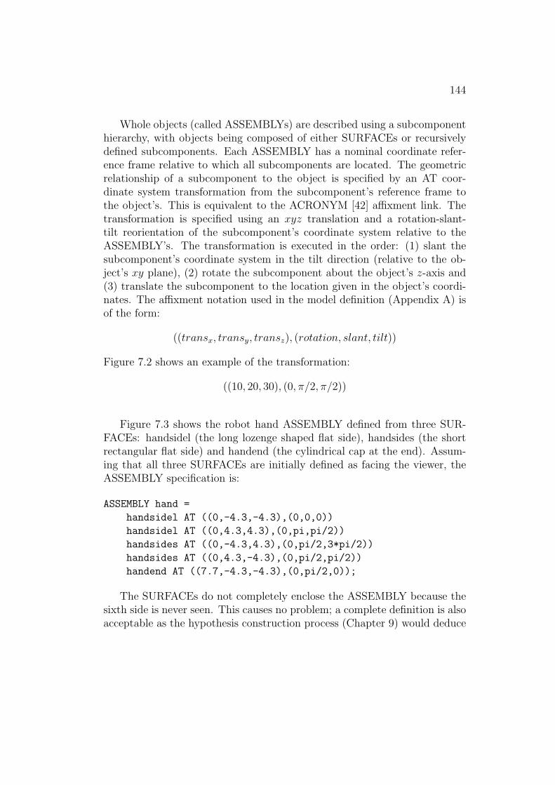
144

Whole objects (called ASSEMBLYs) are described using a subcomponenthierarchy, with objects being composed of either SURFACEs or recursivelydefined subcomponents. Each ASSEMBLY has a nominal coordinate refer-ence frame relative to which all subcomponents are located. The geometricrelationship of a subcomponent to the object is specified by an AT coor-dinate system transformation from the subcomponent’s reference frame tothe object’s. This is equivalent to the ACRONYM [42] affixment link. Thetransformation is specified using an xyz translation and a rotation-slant-tilt reorientation of the subcomponent’s coordinate system relative to theASSEMBLY’s. The transformation is executed in the order: (1) slant thesubcomponent’s coordinate system in the tilt direction (relative to the ob-ject’s xy plane), (2) rotate the subcomponent about the object’s z-axis and(3) translate the subcomponent to the location given in the object’s coordi-nates. The affixment notation used in the model definition (Appendix A) isof the form:

((transx, transy, transz), (rotation, slant, tilt))

Figure 7.2 shows an example of the transformation:

((10, 20, 30), (0, π/2, π/2))

Figure 7.3 shows the robot hand ASSEMBLY defined from three SUR-FACEs: handsidel (the long lozenge shaped flat side), handsides (the shortrectangular flat side) and handend (the cylindrical cap at the end). Assum-ing that all three SURFACEs are initially defined as facing the viewer, theASSEMBLY specification is:

ASSEMBLY hand =

handsidel AT ((0,-4.3,-4.3),(0,0,0))

handsidel AT ((0,4.3,4.3),(0,pi,pi/2))

handsides AT ((0,-4.3,4.3),(0,pi/2,3*pi/2))

handsides AT ((0,4.3,-4.3),(0,pi/2,pi/2))

handend AT ((7.7,-4.3,-4.3),(0,pi/2,0));

The SURFACEs do not completely enclose the ASSEMBLY because thesixth side is never seen. This causes no problem; a complete definition is alsoacceptable as the hypothesis construction process (Chapter 9) would deduce

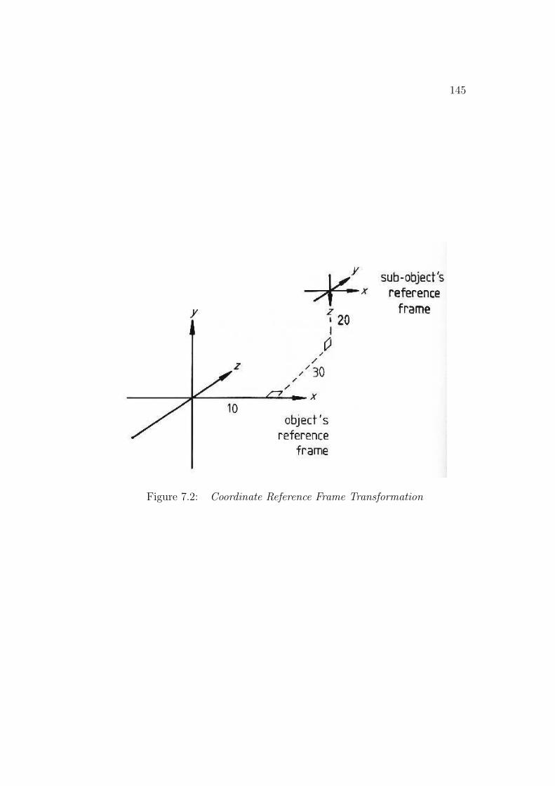
145

Figure 7.2: Coordinate Reference Frame Transformation

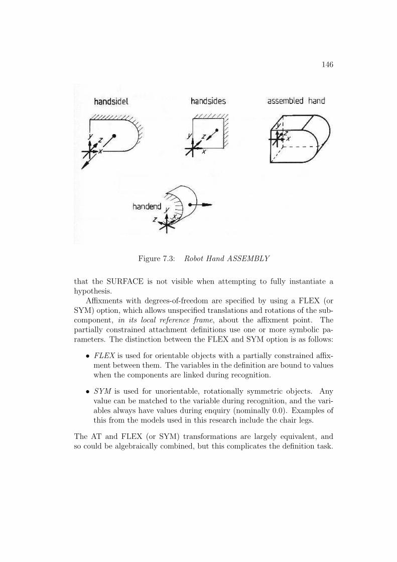
146

Figure 7.3: Robot Hand ASSEMBLY

that the SURFACE is not visible when attempting to fully instantiate ahypothesis.

Affixments with degrees-of-freedom are specified by using a FLEX (orSYM) option, which allows unspecified translations and rotations of the sub-component, in its local reference frame, about the affixment point. Thepartially constrained attachment definitions use one or more symbolic pa-rameters. The distinction between the FLEX and SYM option is as follows:

• FLEX is used for orientable objects with a partially constrained affix-ment between them. The variables in the definition are bound to valueswhen the components are linked during recognition.

• SYM is used for unorientable, rotationally symmetric objects. Anyvalue can be matched to the variable during recognition, and the vari-ables always have values during enquiry (nominally 0.0). Examples ofthis from the models used in this research include the chair legs.

The AT and FLEX (or SYM) transformations are largely equivalent, andso could be algebraically combined, but this complicates the definition task.

147

Figure 7.4: Partially Constrained ASSEMBLY Example

A subcomponent’s partially constrained position is usually specified relativeto the subcomponent, not the ASSEMBLY. The affixment to the ASSEM-BLY, however, is usually about a point that is defined in the ASSEMBLY’sreference frame, so that the two transformations are separated.

An ASSEMBLY S with a rotational degree-of-freedom is shown in Figure7.4. It is attached to the table T and rotates rigidly (to angle Θ) alongthe path CD. S and T are part of ASSEMBLY Q. Both T and Q havetheir coordinate frames located at G and S has its at B. The ASSEMBLY isdefined:

ASSEMBLY Q =

T AT ((0,0,0),(0,0,0)) % T is at G

S AT ((10,0,0),(3*pi/2,pi/2,0)) % from G to A

FLEX ((-7,0,0),(Theta,0,0)); % from A to B

The recursive subcomponent hierarchy with local reference frames sup-ports a simple method for coordinate calculations. Assume that the hierarchyof components is:

ASSEMBLY P0 =

P1 AT A1

148

FLEX F1

ASSEMBLY P1 =

P2 AT A2

FLEX F2

ASSEMBLY P2 =

P3 AT A3

FLEX F3

...

Let Ai and Fi be simplified homogeneous coordinate matrices representingthe reference frame transformations given above. Then, each of these 4*4matrices has the form:

(

Ri~Ti

~0t 1

)

where Ri is the 3 × 3 rotation matrix and ~Ti is the translation vector. Eachmatrix represents the transformation ~Ti +Ri ∗~v of a vector ~v in the subcom-ponent to the object coordinate system. If:

G is the matrix transforming the ASSEMBLY’s top level coordinate systeminto global coordinates, and

C transforms from global coordinates into those of the camera,

then a point ~p in the local coordinate system of ASSEMBLY Pn can beexpressed in camera coordinates by the calculation:

CG(A1F−11 )(A2F

−12 )...(AnF−1

n )~p

There are many ways to decompose a body into substructures, and thisleads to the question of what constitutes a good segmentation. In theory, nohierarchy is needed for rigidly connected objects, because all surfaces could bedirectly expressed in the top level object’s coordinate system. This is neitherefficient (e.g. there may be repeated structure) nor captures our notionsof substructure. Further, a chain of multiple subcomponents with partiallyconstrained affixments represented in a single reference frame would have acomplicated linkage definition.

Some guidelines for the decomposition process are:

1. Object surfaces are segmented according to the shape discontinuitycriteria of Chapter 3.

149

Figure 7.5: Segmenting a Rivet Versus a Cylinder on a Plane

2. Non-rigidly connected substructures are distinct ASSEMBLYs.

3. Repeated structures become distinct ASSEMBLYs (e.g. a commonsurface shape, like a chair leg).

4. Surface groups surrounded by concave surface shape discontinuities be-come ASSEMBLYs (e.g. where the nose joins to the face). This isbecause one cannot distinguish a connecting-to from a sitting-on rela-tionship, and so data segmentation must take the conservative choice.Hence, the models should follow this as well. Figure 7.5 illustrates thisproblem for a structure that might be a rivet or a cylinder on a plane.

Examples of the ModelsA range of solid and laminar structures were modeled. The robot model

(Figure 1.9) has four rigid subcomponents: the cylindrical base, the shoulder,the upper arm and the lower arm/gripper. Each of these is an ASSEMBLY,as are several of their subcomponents. These four components are joinedhierarchically using the FLEX option to represent the partially constrained

150

Figure 7.6: Chair Model

joint angles. The shoulder body and robot body are defined using non-segmenting boundaries to correspond to the observed extremal boundaries(as discussed below).

The chair (Figure 7.6) and trash can (Figure 7.7) illustrate laminar sur-faces and symmetric subcomponents (SYM). The chair legs are defined asthin cylinders, which are attached by a SYM relation to the chair, as is theseat. The seat and back are both laminar surfaces defined using two back-to-back SURFACEs (with their associated surface normals outward-facing). Asimilar construction holds for the trash can. Its model has six SURFACEs,because both the outer and inner cylindrical surfaces were split into two,with non-segmenting boundaries joining.

The complete model for the robot is given in Appendix A.

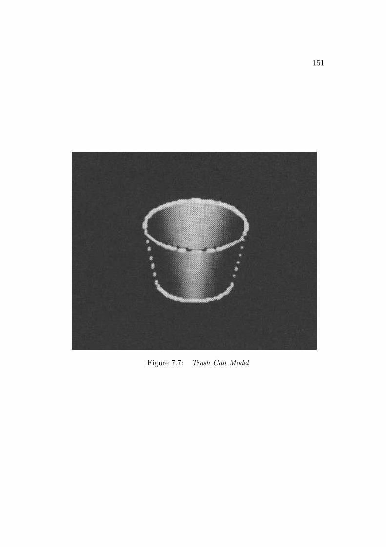
151

Figure 7.7: Trash Can Model

152

Figure 7.8: Chair Leg Becomes Part of Chair Back

Discussion on the Geometric ModelThere are several major inadequacies with the geometric modeling sys-

tem. Object dimensions have to be fixed, but this was largely because no con-straint maintenance mechanism was available (unlike in ACRONYM [42]).Uniform surface and boundary segment curvatures were also simplifications.However, because major curvature changes cause segmentations, deviationsbetween the models and observed objects should be minor. The point wasto segment the models in a similar manner to the data, to promote directfeature matching through having a similar representation for both.

Of course, some surfaces do not segment into conceptual units strictlyon shape discontinuities, such as when a chair leg continues upward to formpart of the chair back (Figure 7.8). Here, the segmentation requires a bound-ary that is not in the data. This is part of the more general segmentationproblem, which is ignored here.

The surface matching process described in Chapter 9 recognizes imagesurfaces by pairing them with model SURFACEs. Because non-planar sur-faces can curve away from the viewer’s line-of-sight, the observed surfacepatch may not correspond to the full modeled patch. Moreover, extremalboundaries will be seen, and these will not correspond with the patch bound-aries.

As the matching process can not properly account for this phenomenon, itwas necessary to ensure that the models were defined to help avoid the prob-

153

lem. This required splitting large curved surfaces into patches correspondingto typically obscured surfaces. For example, full cylindrical surfaces weresplit into two halves, because only one half could be seen from any view-point. The new cylindrical patch boundaries approximately correspond tothe extremal boundaries (i.e. subset of the front-side-obscuring boundaries)of the observed surface.

For surfaces with an extent that distinguishes orientation, this approachneeds extension. A key instance where this splitting was adequate but notgeneral was with the cylindrical robot shoulder, because the shoulder hadan irregular notch where it connected to the base. As with the cylindricalsurface, the patch was split at its apex to give a boundary that could bematched with the observed extremal boundary, and a roughly correspondingsurface patch. If the robot had been viewed from an orientation substantiallyabove or below that actually seen in Figure 1.1, the shoulder patch may nothave been recognized.

Surfaces have been represented with a single boundary, and so must nothave any holes. The important issues of scale, natural variation, surfacetexture and object elasticity/flexibility are also ignored, but this is true ofalmost all modeling systems.

This surface-based representation method seems best for objects thatare primarily man-made solids. Many other objects, especially natural ones,would not be well represented. The individual variation in a tree would not becharacterizable, except through a surface smoothing process that representedthe entire bough as a distinct solid with a smooth surface, over the class ofall trees of the same type. This is an appropriate generalization at a higherlevel of conceptual scale. Perhaps a combination of this smoothing withPentland’s fractal-based representation of natural texture [130] could solvethis problem.

According to the goals of the recognition system, an object probablyshould not be completely modeled, instead only the key features need de-scription. In particular, only the visually prominent surfaces and featuresneed representation and these should be enough for initial identification andorientation.

Finally, any realistic object recognition system must use a variety of rep-resentations, and so the surface representation here should be augmented.Several researchers (e.g. [121, 42, 112]) have shown that axes of elongatedregions or volumes are useful features, and volumetric models are usefulfor recognition. Reflectance, gloss and texture are good surface properties.

154

Viewer-centered and sketch models provide alternative representations.

7.2 Other Model Information

Object models include more than just shape and structure, and this sectiondiscusses the remaining information and its representation. Model invoca-tion (Chapter 8) needs three types of object-linked information. (The workdescribed below is by both myself ([67, 72]) and Paechter [128].) The detailsand the use of this information is described in depth in Chapter 8.

The first type is interobject relationships, which provides indirect evi-dence. Seven types of relationships are allowed: subcomponent, supercom-ponent, supertype (family), subclass (specialization), superclass (simplifica-tion), arbitrary association and inhibiting. The model also includes a weightto express the importance of the relationship. The information is representedas:

relation OF objecttype1 IS objecttype2 weight

For example:

SUPERTYPE OF trash can outer surface IS positive cylinder 1.0

The second requirement is for constraints on feature properties (Chapter6) specified by the acceptable value ranges and a contribution weight. Ex-amples of this information are the expected areas of surfaces or angles atwhich surfaces meet. The value ranges are based on normal distributionsabout peak values, and may include or exclude the values near the peak.Additionally, some properties may just be required to be above (or below)the peak value. Altogether, six forms for property requirements are used.

The final invocation requirement is for subcomponent groups, which arelists of the immediate subcomponents seen from each distinct viewpoint.

Some of the extra information could have been derived from the geo-metric models (e.g. subcomponent relationships). For others, such as theimportance of an attribute to the invocation of a model, the relationships orthe methods for automatically extracting the information (i.e. for decidingon the key visible feature groups) are not well understood. Hence, the extrainformation is represented explicitly.

155

7.3 The SMS Object Representation Approach

Based on the experience of this and more recent research, the SMS ob-ject representation system [70] was designed. Extensions over the geometricmodel approach described above include: multiple, alternative representa-tions (curve, surface or first and second-order volumetric primitives), sur-faces that extend around the objects, and can have holes, key feature mod-els, parameterized feature sizes and properties (e.g. surface curvatures), un-constrained degrees-of-freedom in reference frame transformations, multiplelevels of scale-based representation and viewpoint dependent visibility infor-mation.

The goal of SMS is to represent the visual aspects of an object thatcharacterize its identity, rather than describe its shape. Hence, the modelingapproach aims to provide representations that closely correspond to reliablyextractable image features. This implies that:

1. all object features may not be represented, but instead only the mostsalient,

2. model representations may not be exact enough for precise reconstruc-tion of the object (e.g. shapes may be simplified to correspond toexpected data features or surface patches may not join up neatly) and

3. there may be a variety of alternative (structural or scale-based) repre-sentations, depending on the expected data.

The SMS structural models are linked by a subcomponent hierarchy sim-ilar to that described for IMAGINE I, where subcomponents can be joinedto form larger models by reference frame transformations. SMS allows par-tially constrained relationships, either through the use of variable parametersin the transformation, or by use of an unconstrained degree-of-freedom rela-tionship that, for example, aligns a subcomponent axis vector with a givenvector direction in the main model.

The primitive ASSEMBLY structure (i.e. one without subcomponentASSEMBLYs) can have three non-exclusive representations based on curve,surface or volumetric primitives. The main motivation for the structural al-ternatives is that different sensors produce different data features (e.g. stereoproduces good edge features, ranging produces good surface features andbodyscanners produce good volumetric features). SMS allows one to use the

156

same model to interpret data from all of these scenes; whether this is usefulis not known yet.

The curve representations are piecewise circular, elliptic and straight arcs,segmented by the curvature discontinuity criteria proposed in Chapter 3. Sur-face patches are similar to those described above, except that SURFACEscan now be connected on all sides (e.g. a complete cylinder instead of twoarbitrarily segmented patches) and may have holes. Patches are carved outof infinite planes, cylinders and cones, or (finite) tori. Volumetric primitivesare based on those proposed by Shapiro et al. [146]. They used a rough threedimensional object model based on sticks (one primary dimension of exten-sion), plates (two dimensions) and blobs (three dimensions) and structuralinterrelationships. This approach allowed development of more stable rela-tional models, while still symbolically characterizing object structure. TheSMS modeling system also has some second-order volumetric representations[73] for small positive features (bump, ridge, fin and spike) and negative fea-tures (dent, groove, slot and hole). The volumetric primitives provide modelprimitives that can be matched to rough spatial characterizations of the scene- such as when stereo provides only a sparse depth image.

In Figure 7.9 we can see first a surface characterization of a “widget”and then a volume and curve based model. Each representation approachcaptures the “feel” of the object differently.

There is a simplification hierarchy in SMS, which links together modelsthrough scale relationships. This development is more speculative, and triesto fuse the ideas of Marr and Nishihara [111] and Brooks [42] on scale-basedrefinement of model representations and generalization hierarchies. At eachnew level in the simplification hierarchy, models have their features simplifiedor removed, resulting in broader classes of objects recognizable with themodel. Figure 7.10 shows a coarse and fine scale model of an ashtray (whichis also considerably more free-form than the “widget”). The main differencebetween the two representations is the simplification of the cigarette restcorrugations in the fine scale model to a plane in the coarse model. Theplane is a suitable representation for when the object is too distant from theobserver to resolve the fine detail.

Following ACRONYM [42], all numerical values can be symbolic variablesor expressions, as well as constants. This has been used for generic modelrepresentation, by allowing size variation amongst the recognizable objects.Variables are defined as either local or global to a model and are boundby a dynamic scoping mechanism. For example, one could define a robot

157

Figure 7.9: Surface and Volume/Curve Model of “Widget”

158

Figure 7.10: Coarse and Fine Scale Model of Ashtray

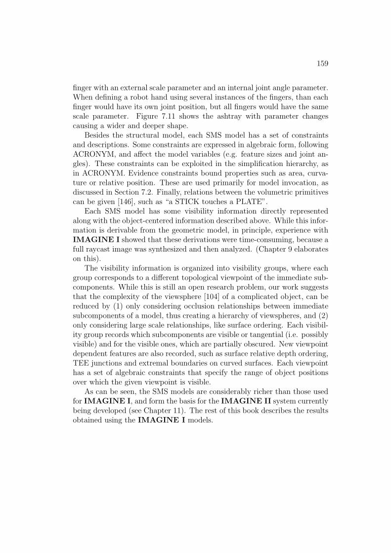
159

finger with an external scale parameter and an internal joint angle parameter.When defining a robot hand using several instances of the fingers, than eachfinger would have its own joint position, but all fingers would have the samescale parameter. Figure 7.11 shows the ashtray with parameter changescausing a wider and deeper shape.

Besides the structural model, each SMS model has a set of constraintsand descriptions. Some constraints are expressed in algebraic form, followingACRONYM, and affect the model variables (e.g. feature sizes and joint an-gles). These constraints can be exploited in the simplification hierarchy, asin ACRONYM. Evidence constraints bound properties such as area, curva-ture or relative position. These are used primarily for model invocation, asdiscussed in Section 7.2. Finally, relations between the volumetric primitivescan be given [146], such as “a STICK touches a PLATE”.

Each SMS model has some visibility information directly representedalong with the object-centered information described above. While this infor-mation is derivable from the geometric model, in principle, experience withIMAGINE I showed that these derivations were time-consuming, because afull raycast image was synthesized and then analyzed. (Chapter 9 elaborateson this).

The visibility information is organized into visibility groups, where eachgroup corresponds to a different topological viewpoint of the immediate sub-components. While this is still an open research problem, our work suggeststhat the complexity of the viewsphere [104] of a complicated object, can bereduced by (1) only considering occlusion relationships between immediatesubcomponents of a model, thus creating a hierarchy of viewspheres, and (2)only considering large scale relationships, like surface ordering. Each visibil-ity group records which subcomponents are visible or tangential (i.e. possiblyvisible) and for the visible ones, which are partially obscured. New viewpointdependent features are also recorded, such as surface relative depth ordering,TEE junctions and extremal boundaries on curved surfaces. Each viewpointhas a set of algebraic constraints that specify the range of object positionsover which the given viewpoint is visible.

As can be seen, the SMS models are considerably richer than those usedfor IMAGINE I, and form the basis for the IMAGINE II system currentlybeing developed (see Chapter 11). The rest of this book describes the resultsobtained using the IMAGINE I models.

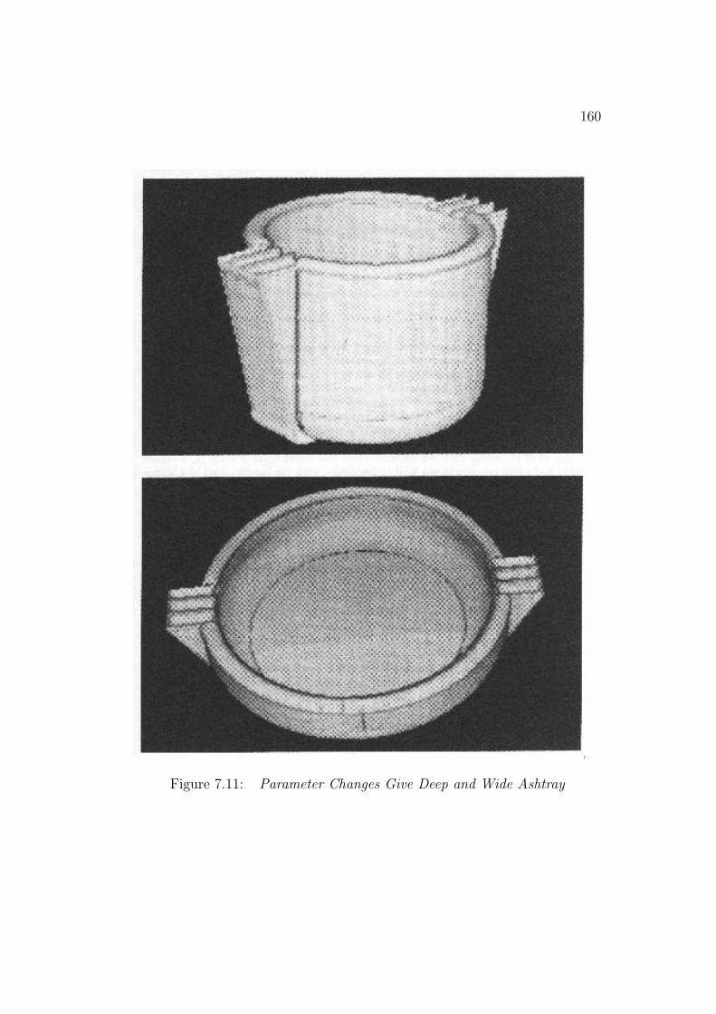
160

Figure 7.11: Parameter Changes Give Deep and Wide Ashtray

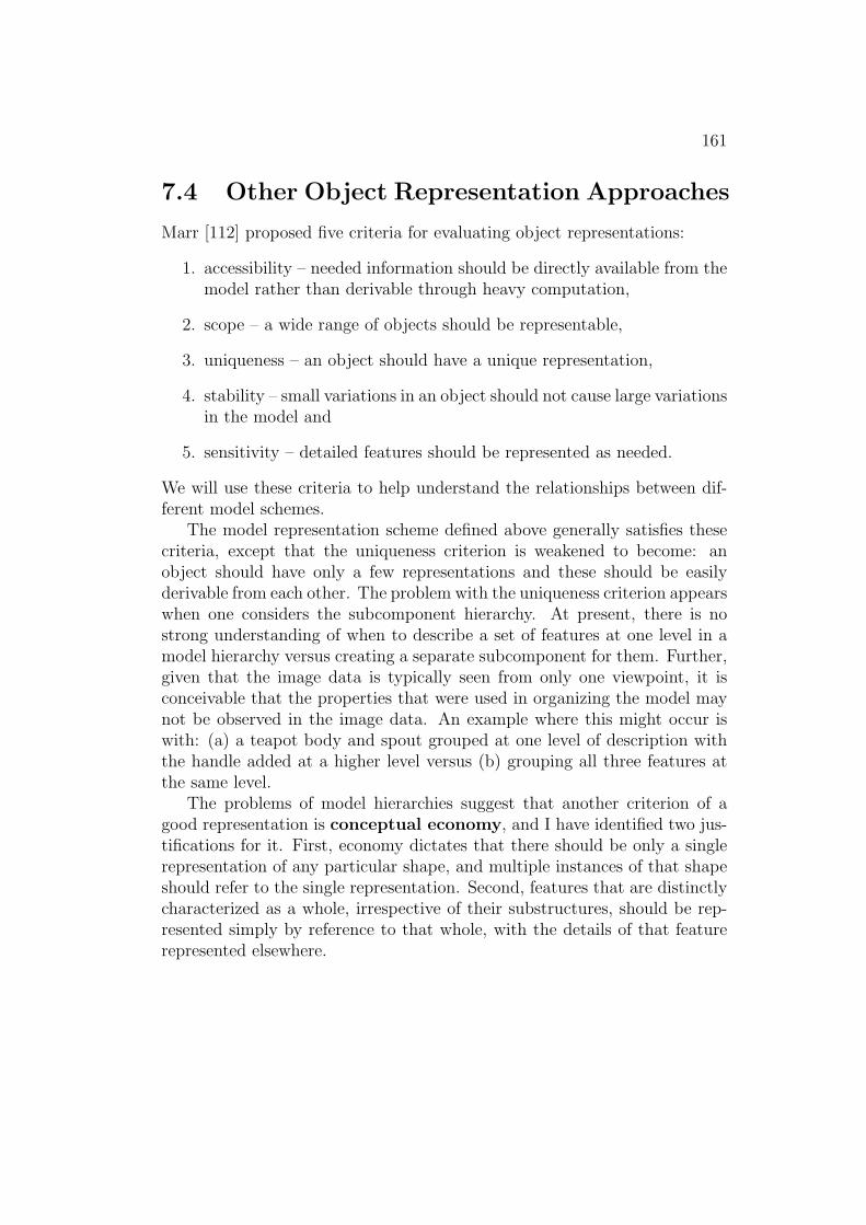
161

7.4 Other Object Representation Approaches

Marr [112] proposed five criteria for evaluating object representations:

1. accessibility – needed information should be directly available from themodel rather than derivable through heavy computation,

2. scope – a wide range of objects should be representable,

3. uniqueness – an object should have a unique representation,

4. stability – small variations in an object should not cause large variationsin the model and

5. sensitivity – detailed features should be represented as needed.

We will use these criteria to help understand the relationships between dif-ferent model schemes.

The model representation scheme defined above generally satisfies thesecriteria, except that the uniqueness criterion is weakened to become: anobject should have only a few representations and these should be easilyderivable from each other. The problem with the uniqueness criterion appearswhen one considers the subcomponent hierarchy. At present, there is nostrong understanding of when to describe a set of features at one level in amodel hierarchy versus creating a separate subcomponent for them. Further,given that the image data is typically seen from only one viewpoint, it isconceivable that the properties that were used in organizing the model maynot be observed in the image data. An example where this might occur iswith: (a) a teapot body and spout grouped at one level of description withthe handle added at a higher level versus (b) grouping all three features atthe same level.

The problems of model hierarchies suggest that another criterion of agood representation is conceptual economy, and I have identified two jus-tifications for it. First, economy dictates that there should be only a singlerepresentation of any particular shape, and multiple instances of that shapeshould refer to the single representation. Second, features that are distinctlycharacterized as a whole, irrespective of their substructures, should be rep-resented simply by reference to that whole, with the details of that featurerepresented elsewhere.

162

Brady [39] proposed three additional criteria for analyzing representationschemes: rich local support, smooth extension and subsumption of repre-sentations and reference frame propagation. Since surface patch types aredefined by the principal curvatures, the first additional criterion is partiallysatisfied. The second one does not seem to apply (Brady investigated merginglocal descriptions to form larger descriptions). The reference frame propaga-tion criterion also seems to be satisfied because, here, all model features havewell defined local reference frames and data descriptions also have local ref-erence frames (though there may be degrees-of-freedom, as with a cylindricalpatch).

Modeling schemes in computer vision mainly belong to two families:

• Property representations – that define objects by properties or con-straints (without recourse to an explicit geometric model) the satisfac-tion of which should lead to unique identification.

• Geometric representations – that represent object shape and structure.

The representations may be expressed implicitly in a computer program orexplicitly as an identifiable defined model. The implicit model is not differentin competence from the explicit model, but is ignored here because of its lackof generality. We discuss the two families in greater detail in the followingsubsections. (These representations are closely related to the matching algo-rithms discussed in Chapter 2.)

Property RepresentationsA typical property representation associates lists of expected properties

with each object. Some examples of this are:

• color, size and height for image regions in office scenes [55],

• rough object sizes, colors and edge shapes for desk top objects [149]and

• face shape, edge lengths and two dimensional edge angles for identifyingpolyhedra [60].

One can also include relationships that have to be held with other structures(e.g. [19]), such as in Adler’s program [3] that interpreted two dimensionalPeanuts cartoon figure scenes.

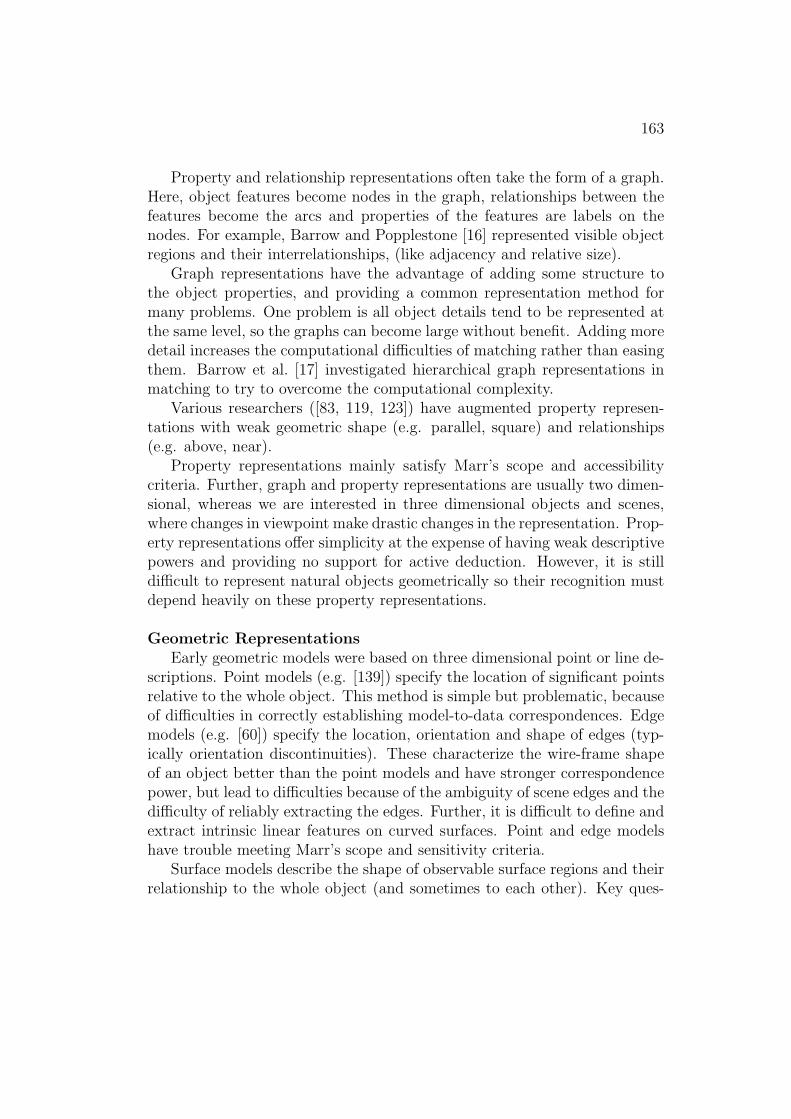
163

Property and relationship representations often take the form of a graph.Here, object features become nodes in the graph, relationships between thefeatures become the arcs and properties of the features are labels on thenodes. For example, Barrow and Popplestone [16] represented visible objectregions and their interrelationships, (like adjacency and relative size).

Graph representations have the advantage of adding some structure tothe object properties, and providing a common representation method formany problems. One problem is all object details tend to be represented atthe same level, so the graphs can become large without benefit. Adding moredetail increases the computational difficulties of matching rather than easingthem. Barrow et al. [17] investigated hierarchical graph representations inmatching to try to overcome the computational complexity.

Various researchers ([83, 119, 123]) have augmented property represen-tations with weak geometric shape (e.g. parallel, square) and relationships(e.g. above, near).

Property representations mainly satisfy Marr’s scope and accessibilitycriteria. Further, graph and property representations are usually two dimen-sional, whereas we are interested in three dimensional objects and scenes,where changes in viewpoint make drastic changes in the representation. Prop-erty representations offer simplicity at the expense of having weak descriptivepowers and providing no support for active deduction. However, it is stilldifficult to represent natural objects geometrically so their recognition mustdepend heavily on these property representations.

Geometric RepresentationsEarly geometric models were based on three dimensional point or line de-

scriptions. Point models (e.g. [139]) specify the location of significant pointsrelative to the whole object. This method is simple but problematic, becauseof difficulties in correctly establishing model-to-data correspondences. Edgemodels (e.g. [60]) specify the location, orientation and shape of edges (typ-ically orientation discontinuities). These characterize the wire-frame shapeof an object better than the point models and have stronger correspondencepower, but lead to difficulties because of the ambiguity of scene edges and thedifficulty of reliably extracting the edges. Further, it is difficult to define andextract intrinsic linear features on curved surfaces. Point and edge modelshave trouble meeting Marr’s scope and sensitivity criteria.

Surface models describe the shape of observable surface regions and theirrelationship to the whole object (and sometimes to each other). Key ques-

164

tions include how to describe the shape of the surfaces and what constitutesan identifiable surface primitive.

Surface regions can be represented by their bounding space curves inwire frame models ([36, 14], page 291). Planar surfaces are most easily rep-resented, but curved surfaces can also be represented by judicious placementof lines. While useful for computer-aided design and graphics, the surfaceinformation needed for recognition tends to be hard to access.

Surface patch models can give arbitrarily accurate representations of ob-ject surfaces. One approach to surface representation is by bicubic splinepatches ([171, 14], page 269), where cubic polynomials approximate the sur-face between fixed control points, giving both positional and derivative con-tinuity. Lack of uniqueness and stability are weak aspects of these models.Also, these modeling approaches ignore the problem of shape discontinuities(i.e. surface orientation).

A second popular approach uses polygonal patches (e.g. [34]), with sub-division of the patches to achieve the required accuracy. These representsurfaces well, but give no conceptual structure to the surface and also sufferover the stability criterion. Faugeras and Hebert [63] used planar patchesderived from depth data to partially bound a three dimensional rigid object.Here, the model did not characterize well the full object, rather, it concen-trated on nearly planar regions. Other researchers have created planar andcylindrical surface models from light-stripe range data (e.g. [133, 52]).

On the whole, surfaces represent the actual visibility of an object welland allow direct comparison of appearance, but do not easily characterize themass distribution of an object. Further, techniques for describing surfacesthat are curved or have natural variation for recognition have not yet beenwell formulated.

Volumetric models represent the solid components of an object in relationto each other or the whole object. Examples include space filling models (e.g.[14], page 280) that represent objects by denoting the portions of space inwhich the object is located, and constructive solid geometry (CSG) models,that start from geometric primitives like cubes, cylinders or half-spaces (e.g.[137, 44]) and then form more complex objects by merging, difference andintersection operations. With these, three dimensional character is directlyaccessible, but appearance is hard to deduce without the addition of surfaceshape and reflectance information. Matching with solids requires findingproperties of images and solids that are directly comparable, such as ob-scuring boundaries and axes of elongation. These volumetric representations

165

tend to meet only Marr’s scope and sensitivity criteria.Recently, Pentland [131] introduced a superquadric-based volumetric model

representation. The advantage of the superquadrics was that a great varietyof primitive volumes can be described using only a few parameters. Naturalappearance was improved by adding fractal-based surface texture afterwards.Larger objects and scenes were formed by scaling and positioning instancesof the primitives. Pentland demonstrated several techniques for locally esti-mating a global superquadric decomposition (from local shape analysis andglobal subsumption) that was particularly effective on elongated features. Healso demonstrated estimation of fractal parameters from local shape spatialfrequency spectra and showed how these could be used to segment textureregions. However, as with the CSG primitives, superquadric models seem tobe more useful for graphics, and appear to have difficulties with uniquenessand access of the correct feature for model matching. This remains an openresearch area.

Another promising volumetric model for computer vision is the general-ized cylinder (or cone) ([27, 111, 6, 91]), which have had their most significantusage in the ACRONYM system [42].

The primitive unit of representation is a solid specified by a cross-sectionalshape, an axis along which to sweep the cross-section and a sweeping ruledescribing how the shape and orientation of the cross-section vary along theaxis.

The axis was the key feature because of its relation to axes directly deriv-able from image data. Many “growth” based natural structures (e.g. treebranches, human limbs) have an axis of elongation, so generalized cylindersmake good models. It also represents many simple man-made objects well,because the manufacturing operations of extrusion, shaping and turning cre-ate reasonably regular, nearly symmetric elongated solids.

In Marr’s proposal [112], objects were described by the dominant modelaxis and the names and placement of subcomponents about the axis. Sub-components could be refined hierarchically to provide greater detail. Thespecification used dimensionless units, which allowed scale invariance, andthe relative values were represented by quantized value ranges that providedboth the symbolic and approximate representation needed for stability tovariation and error.

Brooks [42] used generalized cylinders in the ACRONYM system, wherethey could be directly matched to image boundary pairs (i.e. ribbons). Sub-components were attached by specifying the rotation and translation relating

166

the object and subcomponent reference frames. All primitive or affixmentrelationship specifications could contain variables, but the subcomponentsused in ACRONYM’s airplane example were all rigidly connected to themain model. Hogg [91] used variable attachments to represent joint varia-tion in a human model, with a posture function constraining relative jointposition over time.

For matching, ACRONYM’s geometric models were compiled into a pre-diction graph, where key generalized cylinders became the nodes and place-ment relationships between the cylinders defined the relations. Because theimage data being matched was two dimensional, the prediction graphs rep-resented typical two dimensional views of the objects, derived from the fullthree dimensional geometric model. The advantage of this was that the fullconstraints of the geometric model could be employed in the uniform graphmatching method. Substantial reasoning was needed to derive the predictiongraph from the three dimensional models.

The most important contribution of ACRONYM’s modeling was the useof algebraic constraints that limit the range of model variables in relation toeither fixed values or other variables. An example would be: “the length ofa desk top is greater than the width, but less than twice the width”, whereboth length and width are variable parameters.

Variables and constraints together support generic class models, at leastin structural terms (as opposed to functional). The structural aspects of themodel define the essential components and their attachments, symbolic pa-rameters denote the type of variation and the constraints specify the range ofvariation. The effect of the algebraic constraints is to structure the space of allpossible models with the same logical part relationships into a generalizationhierarchy, where more restrictive constraints define generic specializations ofthe model. Subclasses are defined by more tightly constrained (or constant)parameters, or additional constraints.

A criticism of the generalized cylinder/cone representation concerns itschoice of primitive element. Many natural and man-made objects do nothave vaguely cylindrical components: a leaf, a rock, the moon, a crumplednewspaper, a tennis shoe. Though some aspects of these objects could bereasonably represented, the representation would omit some relevant aspects(e.g. the essential two dimensionality of the leaf), or introduce other irrele-vant ones (e.g. the axis of a sphere). Hence, other primitives should at leastbe included to increase its scope.

167

Secondly, what is perceived is the surface of objects. Hence, it seemsreasonable that the preferential representation for object recognition shouldmake surface-based information explicit. The near-parallel, tangential ob-scuring boundaries of a generalized cylinder (“ribbon”) are reasonable fea-tures for detection, and the orientation of the figure’s spine constrains itsthree dimensional location, but this is about all the information that is eas-ily derivable from the cylinder representation. Surface shape comparisonsare non-trivial, because it is difficult to determine the visible surfaces of thecylinder and what it will look like from a given viewpoint. It is often hardto decide with what model feature an image feature should correspond.

These models are structured, so that they meet the sensitivity criterionand give unique representations. When modeling objects formed from hi-erarchical collections of elongated primitive shapes, the generalized cylindermethod also meets the scope and stability criteria. The key problem of thesemodels is accessibility – it can be hard to deduce much about the appearanceof an object from its volumetric description and much about which model touse from the observed appearance.

These considerations, however, are most relevant when recognizing ob-jects whose three dimensional surface shape and structure is apparent atthe scale of analysis. The ACRONYM examples, aerial photographs of air-port scenes, were largely two dimensional as almost all objects were reducedto laminar surfaces viewed perpendicularly. Hence, treating nearly parallelintensity boundaries as potentially observable extremal boundaries of gener-alized cylinders was appropriate.

The reduction of generics to numerical ranges of parameter values is sim-plistic, although an important first step. Sometimes it is inappropriate: amodel adequate for recognizing a particular type of office chair probablywould not specialize to any other chair. Any chair model that includes mostoffice chairs would probably require a functional definition: seating surfacemeets appropriate back support surface.

Brooks attempted to introduce structural variation through parametervariation, but his solution seems inappropriate. For example, an integervariable ranging from 3 to 6 was used to state that an electric motor had3, 4, 5 or 6 flanges, and a second variable stated that a motor did or didnot have a base by constraining its value to 0 to 1. More complicated al-gebraic inequalities stated that motors with bases have no flanges. Uniformrepresentation is a laudable goal, but these examples suggest that a morepowerful representation should be considered. Hence, the physical variation

168

within a class (i.e. size and affixment variations), that constraints repre-sent well, should be separated from the conceptual relationships involved ingeneralization, where logical/relational constraints would be better.

There has been little work on object representations for non-rigid objects,other than ACRONYM, as just described. Grimson [79] defined and recog-nized piecewise linear two dimensional models that could scale, stretch alongone axis or have subcomponents joined by a revolute joint. Terzopolous etal. [159] described symmetry-seeking models based on deformable paramet-ric tube and spine primitives. The shapes of the models were controlled byenergy constraints on the deformation of the spine, the symmetry of the tubeand the relative position of the two. These models allowed the successful re-construction of three dimensional natural shapes (e.g. a crook-neck squash)from only the two dimensional image contours. It is unclear, however, if thisapproach is suitable for object recognition, because of the many parametersrequired.

Most geometric representations are object-centered, though Minsky [116]proposed a frame representation for recording features visible from typicaldistinct viewpoints, thus adding viewer-centered information. Chakravarty[47] applied this notion in classifying the topologically distinct views of poly-hedral scenes, for use in object recognition. Koenderink and van Doorn [104]considered the application of such ideas to generic smooth objects, by ana-lyzing the discontinuities of occlusion and visibility relationships.

Final Comments This completes our discussion on object representation.Other discussions of three dimensional object representation techniques canbe found in [14, 23, 71]. A particularly thorough review was given by Besl[26] and covers geometric techniques for space-curves, surfaces, volumes andfour dimensional (i.e. moving) objects. His review also summarized well thebasic geometric matching techniques that are typically used with each classof object.

With the models defined in this chapter, we can now start to recognizethe objects in the scene. The recognition process will make heavy use of thesurface-based geometric models, and of the subcomponent hierarchy. Thefirst step of recognition is to select potential models for the image features,which is the topic of the next chapter.

Chapter 8

Model Invocation

One important and difficult task for a general model-based vision systemis selecting the correct model. Model-based vision is computationally in-tractable without reducing the large set of objects that potentially explain aset of data to a few serious candidates that require more detailed analysis.Since there may be 1,000 – 100,000 distinct objects in a competent generalvision system’s range, and even a modest industrial vision system may have100 distinct objects in its repertoire, the problem is too large to undertakemodel-directed comparisons of every known object in every viewpoint. Theproblem remains even if the potentially massive parallelism of the brain orVLSI are considered.

Visual understanding must also include a non-attentive element, becauseall models need be accessible for interpreting all image data. So, the solutionmust consider both efficiency and completeness of access.

There is also a more crucial competence aspect to the problem. A visionsystem needs to be capable of (loosely) identifying previously unseen objects,based on their similarity to known objects. This is required for non-rigidobjects seen in new configurations, incompletely visible objects (e.g. fromocclusion) or object variants (e.g. flaws, generics, new exemplars). Hence,“similar” models must be invoked to help start identification, where “similar”means sharing some features or having an identically arranged substructure.

In view of all these requirements, model invocation is clearly a complexproblem. This chapter presents a solution that embodies ideas on associationnetworks, object description and representation, and parallel implementa-tions. In the first section, the relevant aspects of the problem are discussed.The second presents a theoretical formulation of the proposed solution, the

169

170

third shows examples of the process, the fourth discusses related work, andthe last evaluates the theory.

The work described here builds on the original work by Fisher [67] andmany significant improvements by Paechter [128].

8.1 Some Characteristics of the Invocation

Process

Invocation is Suggestion

Invocation is the result of the directed convergence of clues that suggestidentities for explaining data. On the street, one occasionally sees a personwith a familiar figure, face and style, but who on closer inspection turnsout not to be the acquaintance. The clues suggest the friend, but directexamination contradicts the suggestion.

Invocation also supports the “seeing” of nonexistent objects, as in, e.g.,Magritte’s surrealist paintings, where configurations of features give the im-pression of one object while actually being another. Figure/ground reversalsand ambiguous interpretations such as the vase and faces illusion could oc-cur when multiple invocations are possible, but only a single interpretationis held at any instant, because of mutual inhibition, as suggested by Arbib[9] and others.

Invocation is Mediated by Relationships

Invocation is computed through associations or relationships with otherobjects. The effect is one of suggestion, rather than confirmation. For ex-ample, a red spheroid might suggest an apple, even though it is a cherry.Another example is seen in the Picasso-like picture drawn in Figure 8.1.Though many structural relationships are violated, there are enough sugges-tions of shapes, correct subcomponents and rough relationships for invokinga human face.

While there are many types of relationship between visual concepts, twokey ones are mediated by class and component relationships as discussed be-

171

Figure 8.1: Picasso-like Figure Invokes Human Model

172

low. Other relationship types include context (robots are more often foundin factories than in trees) or temporal (a red traffic light is often seen aftera yellow traffic light). Altogether, the work here integrates eight differentevidence types: subcomponent, supercomponent, subclass, superclass, de-scription (i.e. generic shape), property, general association and inhibiting(i.e. competing).

Associations Have Varying Importances

The importance of a particular feature in invoking a model is a functionof the feature, model, context and viewing system.

Some objects share common features, such as planar faces in blocks worldscenes. Other objects have distinct features, such as the shape of the EiffelTower, an ear or the characteristic blue light used by emergency vehicles.Hence, some features may dramatically reduce the set of potential models.

Context is also important, because the a priori likelihood of discoveringan object influences the importance of a feature. Wheels (generic) whenseen in a garage are more likely cues for automobiles than when seen in abicycle shop. Part (a) of Figure 8.2 shows is a standard pyramid that isunlikely to invoke any models other than its literal interpretation. Yet, inFigure 8.2 part (b), the same pyramid invokes the “nose” model acceptably.Obviously, the context influences the likely models invoked for a structure.The viewing system is also a factor, because its perceptual goals influence thepriorities of detecting an object. For example, industrial inspection systemsoften concentrate on a few distinctive features rather than on the objects asa whole.

Statistical analysis could determine the likelihood of a feature in a givencontext, but is unhelpful in determining the importance of the feature. Fur-ther, because contexts may change, it is difficult to estimate the object andfeature a priori distributions needed for statistical classification. Finally,feature importance may change over time as factors become more or lesssignificant (e.g. contexts can change). Hence, importance assessment seemsmore properly a learning than an analysis problem.

Evidence Starts with Observed Properties

173

Figure 8.2: Pyramid in Face Context Invokes Nose Model

Property evidence is based on properties extracted from the input data.Here, the evidence will be common unary or binary properties. An exampleis surface shape evidence, which may have zero, one or two magnitudes andaxes of curvature.

The properties are absolute measurements constrained by bounds (likeACRONYM [42]). Some properties must lie in a range, such as expectedsurface area. Others are merely required to be above or below a limit, aswhen requiring positive maximum principal curvature. Other property valuesmay be excluded, such as zero principal curvature.

Evidence is acquired in “representative position” [51]. Features that re-main invariant during data acquisition over all observer positions are few(e.g. reflectance, principal curvatures). As this research is concerned withsurface shape properties, the potential evidence is more limited and includesangles between structures, axis orientations, relative feature sizes and rela-tive feature orientations. Invocation features should be usually visible. Whenthey are not, invocation may fail, though there may be alternative invocationfeatures for the privileged viewing positions.

Evidence Comes from Component Relationships

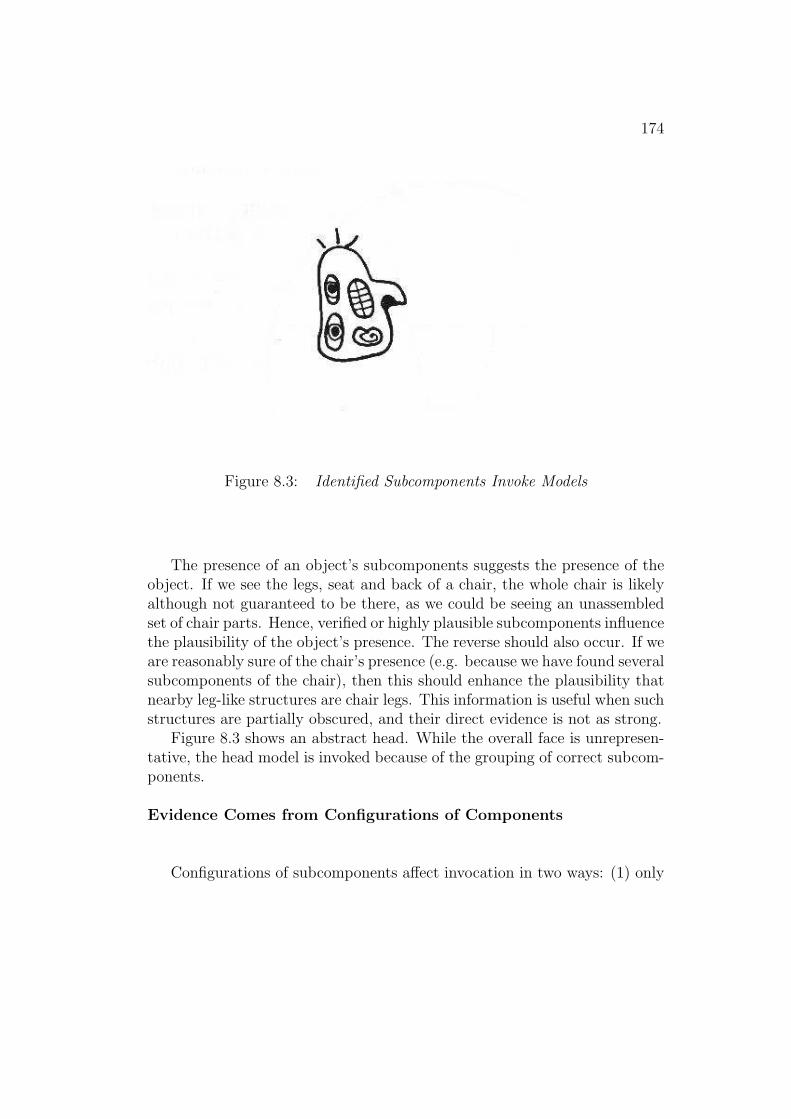
174

Figure 8.3: Identified Subcomponents Invoke Models

The presence of an object’s subcomponents suggests the presence of theobject. If we see the legs, seat and back of a chair, the whole chair is likelyalthough not guaranteed to be there, as we could be seeing an unassembledset of chair parts. Hence, verified or highly plausible subcomponents influencethe plausibility of the object’s presence. The reverse should also occur. If weare reasonably sure of the chair’s presence (e.g. because we have found severalsubcomponents of the chair), then this should enhance the plausibility thatnearby leg-like structures are chair legs. This information is useful when suchstructures are partially obscured, and their direct evidence is not as strong.

Figure 8.3 shows an abstract head. While the overall face is unrepresen-tative, the head model is invoked because of the grouping of correct subcom-ponents.

Evidence Comes from Configurations of Components

Configurations of subcomponents affect invocation in two ways: (1) only

175

a subset of subcomponents is visible from any particular viewpoint, and (2)the spatial distribution of subcomponents can suggest models as well. Thefirst case implicates using visibility groups when integrating evidence. For achair, one often sees the top of the seat and the front of the back support,or the bottom of the seat and back of the back support, or the top of theseat and the back of the back support, but seldom any of the other twelvegroupings of the four subcomponents. These groupings are directly relatedto the major visibility regions in the visual potential scheme suggested byKoenderink and van Doorn [103]. They showed how the sphere of all poten-tial viewing positions of an object could be partitioned according to whatcomponents were visible in each partition and when various features becameself-obscured. Minsky [116] suggested that distinguishable viewer-centeredfeature groupings should be organized into separate frames for recognition.

It is well known that the many small features of a normal object lead to agreat many regions on the view potential sphere. To avoid this problem, twoideas were adopted here. First, rather than creating a new visibility regionwhenever an occlusion event occurs (i.e. when an edge is crossed), the regionsare formed only according to changes in the visibility of large-scale features(i.e. SURFACEs and ASSEMBLYs). That is, a new group is formed when-ever new subcomponents are seen, or when feature ordering relationships aredifferent. Second, the visibility and feature ordering analysis only appliesto the immediate subcomponents of the object, and disregards any visibilityrelationships between their own subcomponents. Thus, visibility complexityis reduced by reducing the number of features and the details of occlusionrelationships considered, by exploiting the subcomponent hierarchy, and byignoring less likely visibility groupings.

Figure 8.4 shows the sphere of viewpoints partitioned into the topologi-cally distinct regions for a trash can. At a particular scale, there are threemajor regions: outside bottom plus adjacent outside surface, outside surfaceplus inside surface and outside, inside and inner bottom surfaces. There areother less significant regions, but these are ignored because of their minorsize.

During invocation, these visibility groupings are used to collect subcom-ponent evidence, and the invocation of a group implies a rough object ori-entation. Here, invocation is the important result, which will lead to initialstructure assignments for hypothesis construction (Chapter 9), from whichorientation is estimated directly.

The second aspect of spatial configurations is how the placement of com-

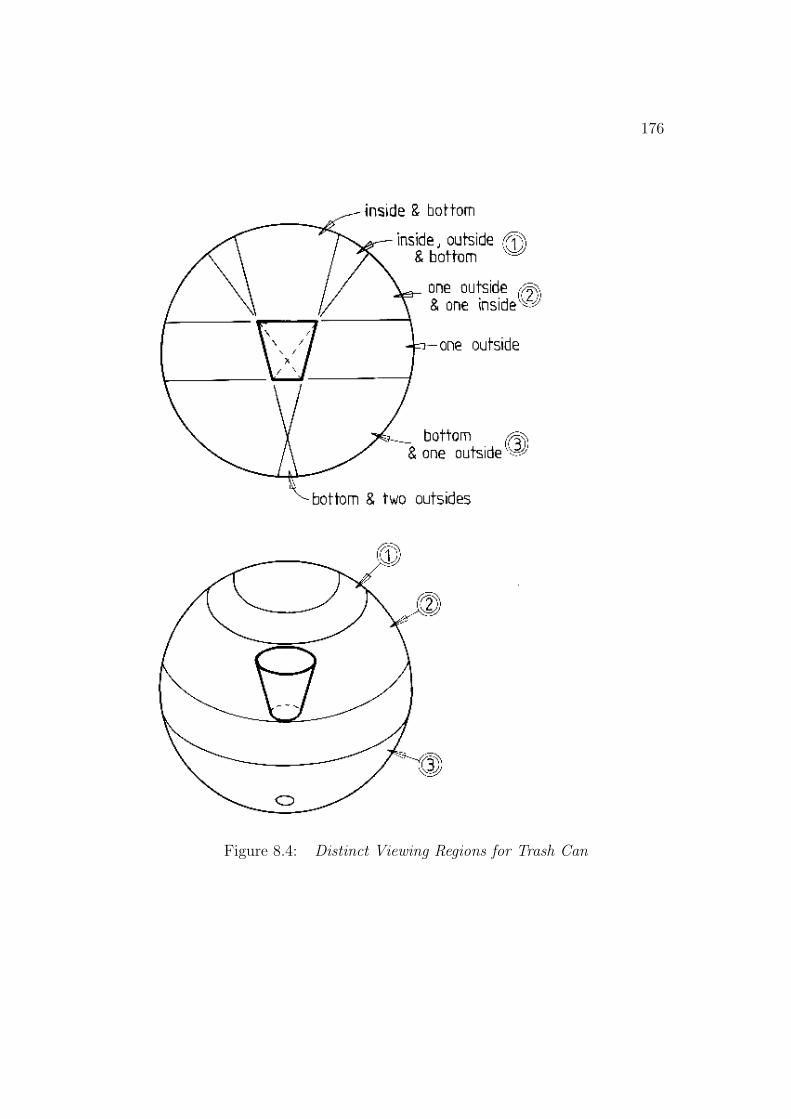
176

Figure 8.4: Distinct Viewing Regions for Trash Can

177

Figure 8.5: Spatial Configurations Invoke Models

ponents, rather than their identity, suggests the model. Figure 8.5 showsthe converse of Figure 8.3, where all subcomponents have the wrong identitybut, by virtue of their position, suggest the face model.

Spatial configuration evidence is represented by binary evidence typesthat constrain relationships like relative position, orientation or size. Theevidence for these relationships should probably be stronger if the featuresinvolved in the relationship also have the correct types. That is, the twoeye-like features in Figure 8.5 help suggest a face, but they would do so morestrongly if they were individually more like eyes.

Evidence Comes from Class Relationships

An object typically has several generalizations and specializations, andevidence for its invocation may come from any of these other hypotheses. Forexample, a generic chair could generalize to “furniture”, or “seating struc-ture”, or specialize to “dentist chair” or “office typing chair”. Because of theunpredictabilities of evidence, it is conceivable that any of the more general-ized or specialized concepts may be invoked before the generic chair. For the

178

more general, this may occur when occlusion leaves only the seating surfaceand back support prominent. Conversely, observation of a particular distin-guishing feature may lead to invocation of the more specific model first. Ineither case, evidence for the categorically related structures gives support forthe structure.

Class prototypes are useful when a set of objects share a common identity,such as “chair”. General properties of an object class are more important forinvocation (as compared to verification, which needs the details of shape).

There are some superficial relationships with the generic identificationscheme in ACRONYM [42], where identification proceeds by descent througha specialization hierarchy with increasingly stringent constraints. Here, thehierarchy and notion of refining constraints are similar, but: (1) the goal issuggestion, not verification, so the property constraints are not strict, and(2) the flow of control is not general to specific: identification could locallyproceed in either direction in the hierarchy.

There is a Low-Level Descriptive Vocabulary

There is a vocabulary of low level, object independent and special inter-mediate shapes and configurations. The purpose of the descriptions is tointroduce generic, sharable structures into the invocation process. Examplesof the symbols include: “positive-cylindrical-surface” and “square-planar-polygon”. However, this vocabulary does not usually refer to identifiablereal objects, but instead to ideal generalizations of some particular aspectsof the object. For the “positive-cylindrical-surface”, it does not say anythingabout the identity of the patch, nor the extent or curvature, but conciselycharacterizes one aspect of the object.

The symbols structure the description of an object, thus simplifying anydirect model-to-data comparisons and increase efficiency through shared fea-tures. A description hierarchy arises from using subdescriptions to definemore complex ones. An example of this is in the chain of descriptions:“polygon” - “quadrilateral” - “trapezoid” - “parallelogram” - “rectangle”- “square”, where each member of the chain introduces a new property con-straint on the previous. The hierarchy helps reduce the model, network andmatching complexity. Rather than specify all properties of every modeledobject, the use of common descriptions can quickly express most propertiesand only object-specific property constraints need be added later.

179

This is important to invocation efficiency, because of the filtering effecton recognitions, whereby image data invoke low level visual concepts, whichthen invoke higher level concepts.

If object descriptions are sufficiently discriminating, a vision system maybe able to accomplish most of its interpretation through only invocation withlittle or no model-directed investigation.

Invocation is Incremental

Evidence can come from a variety of sources and as more supportingevidence accumulates the desirability of invoking a model increases. The in-vocation process must continue even though some evidence is missing becauseof occlusion or erroneous descriptions. Complementary evidence should con-tribute to plausibility and conflicting evidence should detract from it. Theprocess should degrade gracefully: less evidence should lower the desirabilityof invocation rather than prevent it totally.

These factors suggest that invocation is mediated by a continuous plau-sibility.

Invocation Occurs in Image Contexts

There must be contexts for grouping property evidence and for associ-ating subcomponents, so that related evidence is integrated and unrelatedevidence is excluded.

Individual Evidence Values Need to be Integrated

Evidence needs to be integrated several times: when individual propertiesare merged to provide a total property evidence value, when individual sub-component evidence values are combined and when all eight evidence typesare combined. This integration is complicated by the different implications ofthe evidence types and their relative importances. Moreover, the quantity ofevidence associated with different evidence types implies evidence weightingis required.

180

8.2 Theory: Evidence and Association

We now describe the invocation process in detail, based on the intuitions ofthe previous section.

The first consideration of invocation is from its externally viewed char-acteristics – its function and its input and output behavior. Formally, theinputs to invocation are:

• A set {Ci} of image contexts.

• A set {(dj, vij, Ci)} of image descriptions of type (d) with value (v) forthe data in these contexts.

• A database {(ti,Mj,Mk, wijk)} of model-to-model (M) relationships ofdifferent types (t) with weights (w).

• A database {(Mi,{(dij, lij, hij, uij, xij, wij)})} of desired description con-straints for each model, where d is the description type, l is the loweracceptable value for the description, h is the expected peak value, uis the upper acceptable value, x specifies whether the desired value isincluded or excluded in the range and w is a weight.

The basic structural unit of invocation is a model instance for a model Mj inan image context Ci. The output of invocation is a set {(Mj, Ci, pij)} of theplausibility measures for each model instance. This implies that each objecttype is considered for each context. Fortunately, the context formulation hasalready achieved a reduction of information.

Invocation always takes place in an image context. This is because ob-jects are always connected and their features are always spatially close. Thecontext defines where image data can come from and what structures canprovide supporting evidence. For this research, the two types of contextsare the surface hypothesis (Chapter 4) and the surface cluster (Chapter 5),which localize evidence for model SURFACEs and ASSEMBLYs respectively.The surface cluster also groups surfaces and contained surface clusters, so isa suitable context for accumulating subcomponent plausibilities.

Model invocation calculates a plausibility representing the degree to whichan object model explains an image structure. Plausibility is a function of themodel, the data context, the data properties, the desired properties, themodel-to-model relationships, current object hypotheses, and the plausibili-ties of all related model-to-data pairings.

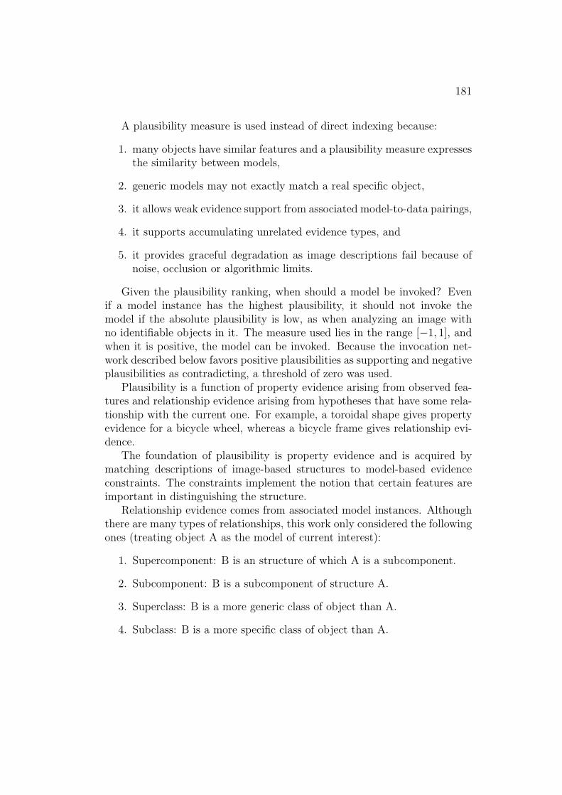
181

A plausibility measure is used instead of direct indexing because:

1. many objects have similar features and a plausibility measure expressesthe similarity between models,

2. generic models may not exactly match a real specific object,

3. it allows weak evidence support from associated model-to-data pairings,

4. it supports accumulating unrelated evidence types, and

5. it provides graceful degradation as image descriptions fail because ofnoise, occlusion or algorithmic limits.

Given the plausibility ranking, when should a model be invoked? Evenif a model instance has the highest plausibility, it should not invoke themodel if the absolute plausibility is low, as when analyzing an image withno identifiable objects in it. The measure used lies in the range [−1, 1], andwhen it is positive, the model can be invoked. Because the invocation net-work described below favors positive plausibilities as supporting and negativeplausibilities as contradicting, a threshold of zero was used.

Plausibility is a function of property evidence arising from observed fea-tures and relationship evidence arising from hypotheses that have some rela-tionship with the current one. For example, a toroidal shape gives propertyevidence for a bicycle wheel, whereas a bicycle frame gives relationship evi-dence.

The foundation of plausibility is property evidence and is acquired bymatching descriptions of image-based structures to model-based evidenceconstraints. The constraints implement the notion that certain features areimportant in distinguishing the structure.

Relationship evidence comes from associated model instances. Althoughthere are many types of relationships, this work only considered the followingones (treating object A as the model of current interest):

1. Supercomponent: B is an structure of which A is a subcomponent.

2. Subcomponent: B is a subcomponent of structure A.

3. Superclass: B is a more generic class of object than A.

4. Subclass: B is a more specific class of object than A.

182

5. Description: Every property of B is a property of A.

6. Inhibition: Identity B competes with identity A.

7. Association: The presence of object B makes the presence of A morelikely.

These seven relationships have been made explicit because each embod-ies different forms of visual knowledge and because their individual evidencecomputations are different. Component relationships give strong circumstan-tial evidence for the presence of objects. An object necessarily requires mostof its subcomponents for it to be considered that object, whereas the reversedoes not hold. The presence of a car makes the presence of wheels highlyplausible, but cannot say much about whether a particular image feature isa wheel. The presence of automobile wheels also makes the presence of a carplausible (though the latter implication is weaker), but does not mean thatany containing image context is likely to contain the car.

The final issue is evidence integration. Evidence is cumulative: each newpiece of valid evidence modifies the plausibility of a structure. Evidence isalso suggestive: each item of support is evaluated independently of the othersand so does not confirm the identity of any structure. Because there are eightdifferent evidence types, the problem of how to compute a single plausibilityvalue arises. We wish to use all the evidence, as data errors, missing values,and object variations are alternative causes for weak evidence, as well ashaving the wrong identity. The solution given below treats the differentevidence values on the same scale, but integrates the values according to theevidence type.

The different model hypotheses in the different contexts are representedas nodes in a network linked by property and relationship evidence arcs.Many of the arcs also connect to arithmetic function nodes that computethe specific evidence values, as discussed in detail below. Property evidenceprovides the raw plausibility values for a few of the nodes, and the other nodesacquire plausibility by value propagation through the relationship arcs.

An abbreviated example is shown in Figure 8.6, where a simplified net-work is shown with the given relationship links (“G” denotes a class rela-tionship, “D” denotes a description relationship, “I” denotes an inhibitingrelationship and “C” denotes a component relationship). The precise formu-lation of the calculations is given in later sections, and the point here is tointroduce the character of the computation (while glossing over the details).

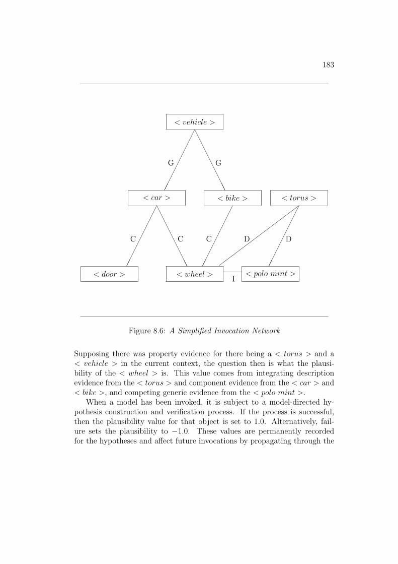
183

< vehicle >

��

��

��

��

��

AAAAAAAAAA

G G

< car >

��

��

��

��

��

AAAAAAAAAA

C C

< bike >

��

��

��

��

��

C

< torus >

��

��

��

��

��

��

��

��

��

��

��

D D

< door > < wheel > < polo mint >I

Figure 8.6: A Simplified Invocation Network

Supposing there was property evidence for there being a < torus > and a< vehicle > in the current context, the question then is what the plausi-bility of the < wheel > is. This value comes from integrating descriptionevidence from the < torus > and component evidence from the < car > and< bike >, and competing generic evidence from the < polo mint >.

When a model has been invoked, it is subject to a model-directed hy-pothesis construction and verification process. If the process is successful,then the plausibility value for that object is set to 1.0. Alternatively, fail-ure sets the plausibility to −1.0. These values are permanently recordedfor the hypotheses and affect future invocations by propagating through the

184

network.In the discussion of each of the relationship types below, three major as-

pects are considered: the type of relationship, the calculation of the relation-ship’s invocation contribution and the context from which the relationshipevidence is taken.

8.2.1 Property Evidence

Property evidence is calculated by evaluating the fit of structural properties(Chapter 6) to model requirements (Chapter 7). An example of a set ofrequirements would be a particular surface must be planar and must meetall adjacent connected surfaces at right angles.

There is some controversy over what constitutes evidence, but here, evi-dence is based only on primitive image properties, such as relative curve ori-entation, rather than higher level descriptions, such as “rectangular”. Thisdecision is partly made because “rectangular” is a distinct conceptual cat-egory and, as such, would be included as a distinct generic element in theinvocation network. It would then have a description relationship to thedesired model.

The context within which data is taken depends on the structure forwhich property evidence is being calculated. If it is a model SURFACE,then properties come from the corresponding surface hypothesis. If it isan ASSEMBLY, then the properties come from the corresponding surfacecluster.

Unary evidence requirements are defined in the model database in oneof six forms, depending on whether the values are required or excluded, andwhether there are upper, lower or both limits on their range. The completeforms are (where e=evidence type is the type of evidence):

185

central include:UNARYEVID low < e < high PEAK peak WEIGHT wgt

above include:UNARYEVID low < e PEAK peak WEIGHT wgt

below include:UNARYEVID e < high PEAK peak WEIGHT wgt

central exclude:UNARYEVID low < e < high PEAK peak ABSENT WEIGHT wgt

above exclude:UNARYEVID low < e PEAK peak ABSENT WEIGHT wgt

below exclude:UNARYEVID e < high PEAK peak ABSENT WEIGHT wgt

If the peak value is the mean of the upper and lower limit, it need not bespecified. Each requirement has a weight that scales the contribution of thisevidence in the total property evidence evaluation.

Binary evidence requirements are defined similarly, with the key differencethat the model also specifies the types of the substructures between whichthe properties are to hold. The model specification for the binary “centralinclude” form is:

BINARYEVID low < evidence_type(type1,type2) < high PEAK peak WEIGHT wgt

In IMAGINE I, all evidence types were considered to be unary. If abinary property between two features was expressed, then evidence evalua-tion would take the best instance of the binary relationship. IMAGINE IImade the relationship explicit. The properties used in IMAGINE I were:

186

NUMLINB number of straight lines in boundaryNUMARCB number of curves in boundaryDBPARO number of groups of parallel lines in boundaryNUM90B number of perpendicular boundary junctionsNUMEQLB number of groups of equal length boundary segmentsDCURV boundary segment curvatureDCRVL boundary segment lengthDBRORT boundary segment relative orientationMINSCURV minimum surface curvatureMAXSCURV maximum surface curvatureSURSDA relative surface orientationABSSIZE surface areaRELSIZE percent of surface area in surface clusterSURECC eccentricity of surface

It is possible to generate automatically most of the evidence types fromthe geometric models, if heuristics for setting the ranges and weight valuesare given, but all these values were manually chosen here. Appendix A showssome of the evidence constraints for the modeled objects.

Models inherit evidence from their descriptions (discussed in Section8.2.4), so only additional evidence (i.e. refinements) need be specified here.

Finally, we consider how the total evidence value is calculated from theindividual pieces of evidence. The constraints on this computation are:

• Each piece of evidence should contribute to the total value.

• The contribution of a piece of evidence should be a function of itsimportance in uniquely determining the object.

• The contribution of a piece of evidence should be a function of thedegree to which it meets its constraints.

• Negative evidence should inhibit more strongly than positive evidencesupport.

• Each piece of evidence should only be evaluated by the best fittingconstraint (allowing disjunctive evidence constraints).

• All constraints need evidence.

• Every property must meet a constraint, if any constraints of the ap-propriate type exist.

187

• Not all properties are constrained (i.e. some are irrelevant).

• Binary property evaluations are also a function of the plausibility thatthe two substructures have the desired identities.

Based on the “degree of fit” requirement, a function was designed toevaluate the evidence from a single description. The function is based on ascaled gaussian evaluation model, with the evaluation peaking at the desiredvalue, having positive value within the required range (which need not besymmetric), and tailing off to -1.0. Because there are six types of evidencerequirements, six different evidence evaluation functions are needed. How-ever, the excluded types are the negatives of the included types, and thebelow types are the mirror image of the above types. So, only the “centralinclude” and “above include” are described here. Based on the model defi-nitions above, the “central include” function for the ith evidence constraintis:

Let;dj = jth data value

If: dj > peaki

then: fij = ( (dj−peaki)

(highi−peaki)∗ 1.1774)2

else: fij = ( (peaki−dj)

(peaki−lowi)∗ 1.1774)2

And the evaluation ej is:

gij = 2 ∗ exp(−fij

2) − 1

The constant 1.1774 ensures the evaluation equals 0 when the data valueequals high or low. The “above include” function for the ith evidence con-straint is:

Let:dj = jth data value

If: dj > peaki

then: fij = 0.0

else: fij = ( (peaki−dj)

(peaki−lowi)∗ 1.1774)2

And the evaluation ej is:

gij = 2 ∗ exp(−fij

2) − 1

Figure 8.7 illustrates these functions. Their gaussian form is appealing

188

because it is continuous and smooth and relates well to gaussian error distri-butions from property estimation. Other functions meet the requirements,but stronger requirements could not be found that define the function moreprecisely.

A property constraint’s evaluation is given by the data value that bestsatisfies the constraint. This is because model-to-data correspondences havenot been made yet, so the evaluations are undirected. As the point of invo-cation is suggestion, any datum within the constraint range is contributoryevidence, and correct models will have all their constraints satisfied. Hence,the final evidence value for this constraint is given by:

ei = maxj(gij)

This portion of the invocation network is illustrated in Figure 8.8.The evaluation of binary property evidence takes into account the plau-

sibility of the subcomponents as well as the property value itself. Thus:

habi = c1 ∗ gi(a, b) + c2 ∗ par + c2 ∗ pbs + c3

is the evidence evaluation function for the ith binary evidence constraint,relating model subcomponent r to model subcomponent s, when using thevalue of the given property between data features a and b. gi(a, b) is thesame evaluation function as for the unary properties (gij), par and pbs arethe plausibilities that data feature a has model identity r, data feature b hasmodel identity s, and c1, c2 and c3 are constants that express the relativeimportance of the different terms (c1 = 0.8, c2 = 0.4, c3 = −0.6). The finalbinary property evidence value is:

ei = maxab(habi)

This picks the best evidence over all pairs of immediate subfeatures in thedata context.

The evaluations for individual property requirements then need to beintegrated. One function that satisfies the evidence integration constraintsis a weighted harmonic mean:

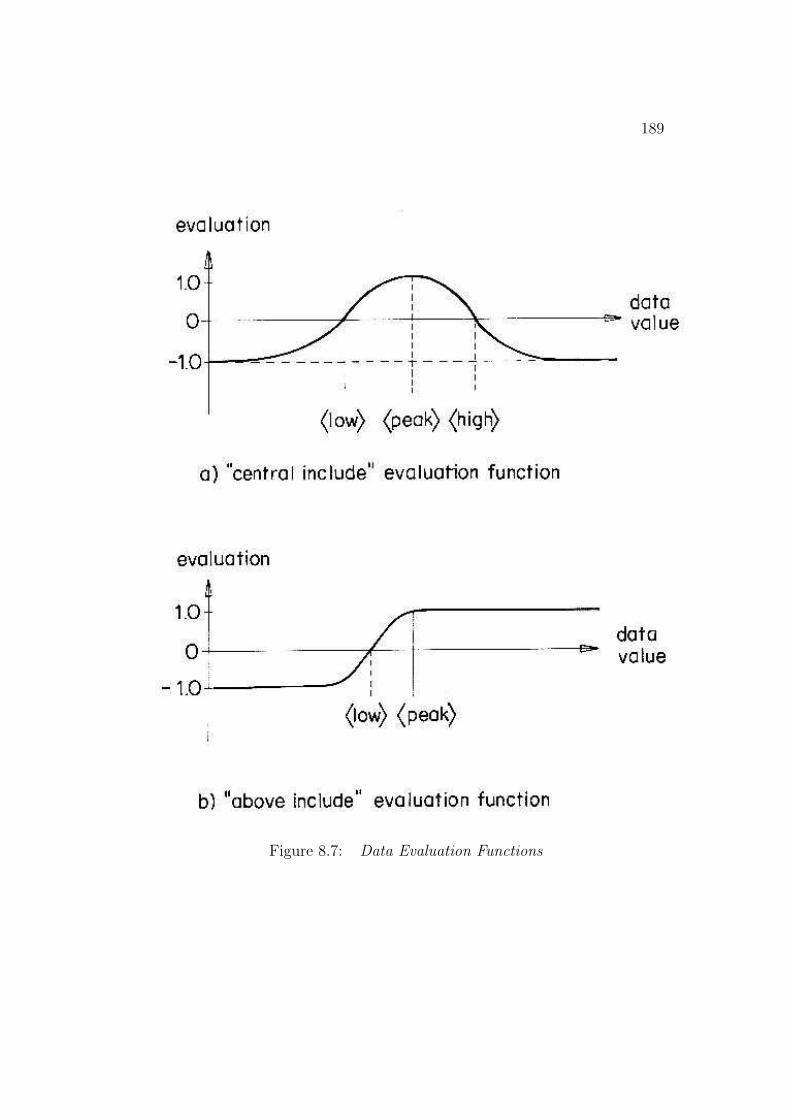
189

Figure 8.7: Data Evaluation Functions

190

Figure 8.8: Best Evaluation Selection Network Fragment

191

let:ei be the data evaluation for the ith property constraintwi be the weight for that evidence type

Then:evdprop = harmmean({(ei, wi)})

whereA =

∑

wi

B =∑ wi

ei+2

harmmean({(ei, wi)}) = AB− 2

If no property evidence is available, this computation is not applied. Themodified harmonic mean is continuous, gives additional weight to negativeevidence and integrates all values uniformly. Moreover, it has the propertythat:

harmmean({(e1, w1), (e2, w2), (e3, w3)})= harmmean({(e1, w1), (harmmean({(e2, w2), (e3, w3)}), w2 + w3)})

This means that we can add evidence incrementally without biasing theresults to the earlier or later values (provided that we also keep track of theweighting of the values). The offset of 2 is used to avoid problems when theplausibility is near -1, and was chosen because it gave good results. Theintegrated property evidence has a weight that is the sum of the individualproperty weights: wprop =

∑

wi.This harmonic mean can be implemented in a value passing network, as

shown in Figure 8.9, which integrates the evidence values ei with weightswi. Here, the square boxes represent unary or binary arithmetic units of thedesignated type, and circular units represent either constants, or the evidencevalues imported from the above calculation.

8.2.2 Supercomponent Associations

This relationship gives evidence for the presence of an object, given the pres-ence of a larger object of which it may be a subpart. Though evidencetypically flows from subcomponents to objects, supercomponent evidencemay be available when: (1) the supercomponent has property or relationshipevidence of its own, or (2) other subcomponents of the object have been

192

Figure 8.9: Harmonic Mean Network Fragment Integrating Property Evi-dence

193

found. Unfortunately, the presence of the supercomponent implies that allsubcomponents are present (though not necessarily visible), but not that animage structure is any particular component. As the supercomponent ev-idence (during invocation) cannot discriminate between likely and unlikelysubcomponents in its context, it supports all equally and thus implements a“priming” operation. This is because the computation is one of plausibility,not certainty. Weighting factors control the amount of support a structuregets. When support is given for the wrong identities, other evidence contra-dicts and cancels this evidence.

There are several constraints derivable from the problem that help definethe evidence computation. They are:

• The presence of a supercomponent makes the presence of an objectplausible.

• The more plausible the presence of the supercomponent, the more plau-sible the presence of the object.

• There is at most one supercomponent of any object, though there maybe many candidates.

• The context of the supercomponent must contain the context of theobject.

The formal definition of the supercomponent relationship computation is:Given:

a model instance of type M in image context Ca set {Si} of supercomponents of Ma set {Cj} of supercontexts of C, including C itself andpij is the plausibility that model Mi occurs in context Cj

Then:fi = maxj(pij)

chooses the best evidence for a supercomponent over all supercontexts andevdsupc = maxi(fi)

picks the best supercomponent evidence over all supercomponent types.The current context is also included because the supercomponent may nothave been visually segmented from the object. If no supercomponent evi-dence is defined or observed, this computation is not applied.

194

The network created for this evidence type is simply a tree of binary“max” units linked as defined above.

8.2.3 Subcomponent Associations

This relationship gives direct evidence for the presence of an object, giventhe presence of its subcomponents. It is stronger than the supercomponentrelationship, because the subcomponents are necessary features of the ob-jects, but it is not a complete implication because the subcomponents maybe present without the presence of the assembled object. The computationdescribed below only requires the presence of the subcomponents and doesnot consider their geometric relations.

This computation is defined by several constraints:

• The more subcomponents present, the more plausible is the object’spresence.

• Even if all subcomponents are present, this does not guarantee thepresence of the object.

• Subcomponents are typically seen in viewpoint dependent groupings,and are seen from only one viewpoint at a time.

• The more plausible a subcomponent’s presence, the more plausible isthe object’s presence.

• The context of all subcomponents must lie within the context of theobject.

The computation is formalized below and looks for the most plausiblecandidate for each of the subcomponents in the given context, and aver-ages the subcomponent’s contributions towards the plausibility of the objectbeing seen from key viewpoints. The final plausibility is the best of the view-point plausibilities. Each of the individual contributions is weighted. Theaveraging of evidence arises because each subcomponent is assumed to givean independent contribution towards the whole object plausibility. Becauseall subcomponents must lie within the same surface cluster as the object,the context of evidence collection is that of the hypothesis and all containedsubcontexts.

The formal definition of the subcomponent relationship calculation is:

195

Given:a model instance of type M in image context Ca set {(Si, wi)} of subcomponents of M ,

where wi is the weight of subcomponent Si

sets Gk = {Ski} of subcomponents representing groupsof subcomponents visible from typical viewpoints

a set {Cj} of subcontexts of the context C including C itselfa set of model instances of type Si, in context Cj,

with plausibility value pij

The weight factors designate significance within the group, with largerweights emphasizing more important or significant features. The subcompo-nent weights are the sum of the weights of the property evidence specifiedfor the subcomponents.

The first value calculated is the best evidence for each subcomponenttype in the subcontexts:

bi = maxj(pij)

This is implemented as a tree of binary “max” units. Then, the evidencefor each viewpoint is calculated by integrating the evidence for the expectedviewpoints using the modified harmonic mean function described above:

vk = harmmean({(bi(k), wi(k))})over all i(k) subcomponents in Gk.

Finally, the evidence from the different viewpoints is integrated, by se-lecting the best evidence:

evdsubc = maxk(vk)

The assumption is that if the object is present, then there should be exactlyone visibility group corresponding to the features visible in the scene. Sub-component evidence has a weighting that is the maximum visibility group’sweight, which is the sum of the weights of the subcomponents and theirproperties:

wsubc = maxk(∑

wi(k))

Relative importances between subcomponents and properties can be modifiedby scaling the relevant weights. The network structure for this computation issimilar to those previously shown. If no subcomponent evidence is available,this computation is not applied.

196

8.2.4 Description Evidence

This relationship gives direct evidence for an object, because all properties ofthe description type (i.e. a generic objects) are also object properties – thetype is a description of the object. The object may have several descriptiontypes: a “square” is both a “rectangle” and a “rhombus”. Hence, evidencefor a description type is also evidence for an object that uses the description,and this is expressed by a plausibility relationship.

Constraints that help specify the description evidence computation are:

• The more plausible the description, the more plausible the object.

• Each description gives additional evidence for an object.

• A weight expresses the importance of the description relative to otherproperty evidence.

• The context of the description is that of the object.

Formally, the description evidence computation is defined:

Given:a model instance of type M in image context Ca set {(Di, wi)} of descriptions Di of M with associated weights wi

a set {pi} of plausibilities of description Di in context C

Then, using the modified harmonic mean, the description evidence is:evddesc = harmmean({(pi, wi)})

The resulting weight of evidence is:wdesc =

∑

wi

If no description types are defined, this computation is not applied. Theportion of the network associated with this evidence is similar to those shownabove.

8.2.5 Superclass Evidence

This relationship gives evidence for the presence of an object of class M ,given the presence of an object of superclass S. For example, evidence for the

197

object being a wide-bodied aircraft lends some support for the possibility ofit being a DC-10. The use of superclass is not rigorous here – the notionis of a category generalization along arbitrary lines. Hence, a class mayhave several generalizations: an < automobile wheel > may generalize to< torus − like object > or < automobile part >. Class generalization doesnot require that all constraints on the generalization are satisfied by thespecialization, which differentiates this evidence type from the descriptionrelationship. So, a superclass need not be a strictly visual generalization,that is, there may be different models for the object and its superclass.

Superclasses provide circumstantial, rather than direct, evidence as thepresence of the < torus − like object > alone does not provide serious ev-idence for the < wheel > being present. If the object had both strong< torus > and < automobile part > evidence, the implication should bestronger. If the object had strong < torus > and weak < automobile part >evidence, then it would be less plausible for it to be a < automobile wheel >.Because the superclass is a generalization, its plausibility must always be atleast as great as that of the object. Hence, the evidence for an object can beat most the minimum of the evidence for its superclasses.

Constraints that help specify the superclass evidence computation are:

• The presence of a superclass increases the plausibility of the object’spresence.

• The more plausible the superclass, the more plausible the object.

• The plausibility of an object is less than that of a superclass.

• The context of the superclass is that of the object.

These constraints lead to the following formal definition of the superclassevidence computation:

Given:a model instance of class M in image context Ca set {Si} of superclasses of Ma set {pi} of plausibilities of model Si in context C

Then, the superclass evidence is:evdsupcl = mini(pi)

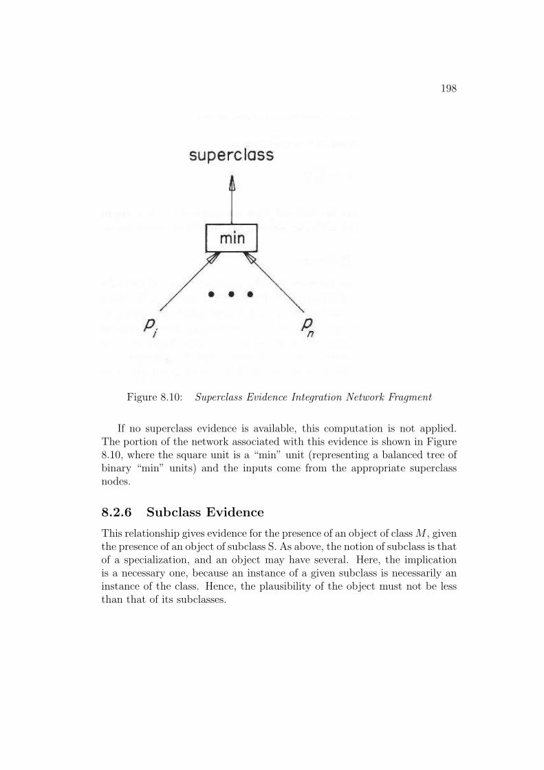
198

Figure 8.10: Superclass Evidence Integration Network Fragment

If no superclass evidence is available, this computation is not applied.The portion of the network associated with this evidence is shown in Figure8.10, where the square unit is a “min” unit (representing a balanced tree ofbinary “min” units) and the inputs come from the appropriate superclassnodes.

8.2.6 Subclass Evidence

This relationship gives evidence for the presence of an object of class M , giventhe presence of an object of subclass S. As above, the notion of subclass is thatof a specialization, and an object may have several. Here, the implicationis a necessary one, because an instance of a given subclass is necessarily aninstance of the class. Hence, the plausibility of the object must not be lessthan that of its subclasses.

199

The constraints that specify the subclass relationship calculation are:

• The more plausible the subclass, the more plausible the object.

• The plausibility of the object is at least that of each subclass.

• The context of the subclasses is the context of the object.

These constraints lead to the following formal definition of the subclassevidence computation:

Given:a model instance of class M in image context Ca set {Si} of subclasses of Ma set {pi} of plausibilities of model Si in context C

Then, the subclass relationship evidence value is:evdsubcl = maxi(pi)

If no subclass evidence is available, this computation is not applied. Theinvocation network fragment for this evidence type is similar to those shownpreviously.

8.2.7 General Associations

This relationship gives evidence for the presence of an object of type M ,given the presence of an object of arbitrary type S. This is not a structureor class relationship, which have already been considered in Sections 8.2.2,8.2.3, 8.2.5 and 8.2.6. It is an “other relationships” category. An relationshipof this type might be: “the presence of a desk makes the presence of a chairplausible”. This allows many forms of peripheral evidence and can be thoughtof as a “priming” relationship.

Association is not commutative, so individual connections need to bemade, if desired, for each direction. For example, the presence of a carmakes the presence of a road likely, whereas there are many roads withoutcars. On the other hand, the evidence supplied is weak: the certain presenceof the car does not necessarily mean the object under consideration is a road.Further, the strength of association will depend on the objects involved.

200

The previous evidence types have clearly specified contexts from whichevidence came, but this type does not. Generally associated objects couldbe anywhere in the scene, so all nodes of the desired type give support.

Some constraints on this type of relationship are:

• The presence of an associated object increases the plausibility of theobject.

• The more plausible the associated object, the more plausible the object.

• The weight of an association expresses the expectation that the desiredobject is present, given that the associated object is present.

• The context of the association is the whole image.

These constraints lead to the following formal definition of the generalassociation computation:

Given:a model instance of type M in image context Ca set {(Si, wi)} of associated models

(where wi is the strength of association)a set {Cj} of all contextsa set {pij} of plausibilities of model Si in context Cj

Then, the association relationship evidence is:evdass = maxi(wi ∗ maxj(pij))

which chooses the best evidence for each associated type, and then thebest weighted association type. If no association evidence is available, thiscomputation is not applied. The invocation network fragment for this evi-dence type is shown in Figure 8.11, where the “max” units represent balancedtrees of binary “max” units and the pij come from other nodes, as describedabove.

8.2.8 Identity Inhibition

A structure seldom has more than one likely identity, unless the identitiesare related (e.g. a structure that is likely to be a DC-10 can also be a wide-bodied aircraft but seldom a banana). Hence, an identity should be inhibited

201

Figure 8.11: Association Evidence Network Fragment

202

by other unrelated identities having high plausibilities in the same context.A second source of inhibition comes from the same identity in subcontexts,to force invocation to occur only in the smallest satisfactory context. Thekey questions are what types provide inhibition, how to quantify the amountof inhibition and how to integrate this inhibition with the other evidencetypes.

Type-related inhibition is a complicated issue. Competition does not al-ways occur even between unrelated generic types. For example, the generictype “positive-cylindrical-surface” should not compete with the generic type“elongated-surface”, whereas it should compete with the generic type “negative-cylindrical-surface”. The latter comparison is between two members of a setof related types that also include: “planar”, “positive-ellipsoid”, “negative-ellipsoid” and “hyperboloid” surfaces. All types in this set compete witheach other, but not with any other types.

Inhibition results in a plausibility value like those discussed in previoussections and is then integrated with the other evidence types, as discussedbelow. An advantage to this method is that it still allows for alternative inter-pretations, as in the ambiguous duck/rabbit figure (e.g. [9]), when evidencefor each is high enough.

Some constraints on the inhibition computation are:

• Inhibition comes from the same type in subcontexts.

• All members of specified sets of generic descriptions inhibit each other.

• All subcomponents and supercomponents of the object do not inhibitthe object.

• All types of the same category (SURFACE or ASSEMBLY) that arenot component, description or class related inhibit each other.

• Only positive evidence for other identities inhibits.

• The inhibition should be proportional to the plausibility of the com-peting identity.

• The inhibition should come from the strongest competition.

• The context of inhibition is the current context for competing identitiesand all subcontexts for the same identity.

203

These constraints lead to the inhibition computation:

Given:a model instance of type M in image context Ca set {Si} of all identities competing with Ma set {Cj} of subcontexts of context Ca set {pi} of plausibilities for the identities Si in context Ca set {pj} of plausibilities for the identity M in the subcontexts Cj

Then, the inhibition evidence is:evdinh = max(maxi(pi),maxj(pj))

This computation gives no inhibition if no competing identities exist.If several identities have roughly equal plausibilities, then inhibition will

drive their plausibilities down, but still leave them roughly equal. A singlestrong identity would severely inhibit all other identities. Figure 8.12 showsthe invocation network unit for computing the inhibition evidence, wherethe lower “max” units represent balanced trees of binary “max” units andthe pi come from competing identities and the pj come from subcontexts, asdescribed above.

8.2.9 Evidence Integration

There are eight evidence types, as discussed in the previous eight sections,and a single integrated plausibility value needs to be computed from them.All values are assumed to be on the same scale so this simplifies the consid-erations.

Some constraints the computation should meet are:

• Directly related evidence (property, subcomponent and description)should have greater weight.

• If there is no property, description or subcomponent evidence, thenevidence integration produces no result.

• Other relationship evidence should be incremental, but not overwhelm-ingly so.

• Only types with evidence are used (i.e. some of the evidence types maynot exist, and so should be ignored).

204

Figure 8.12: Inhibition Invocation Network Fragment

205

• Property, description and subcomponent evidence are complementaryin that they all give explicit evidence for the object and all should beintegrated.

• If supercomponent evidence is strong, then this gives added support fora structure being a subcomponent. Weak supercomponent evidence hasno effect, because the subcomponent could be there by itself, or not bethere at all.

• If superclass evidence is strong, then this gives added support for theobject.

• Strong association evidence supports the possibility of an object’s pres-ence.

• If other identities are competing, they reduce the plausibility.

• As subclasses imply objects, the plausibility of an object must be atleast that of its subclasses.

Based on these constraints, the following integration computation hasbeen designed:

206

Let:evdprop, evddesc, evdsubcl, evdsupcl, evdsubc, evdsupc, evdass, evdinh

be the eight evidence values, with weightings:wprop, wdesc, wsubc

Then:v1 = harmmean({(evdprop, wprop), (evddesc, wdesc), (evdsubc, wsubc)})if evdsupc > 0

then v2 = v1 + csupc ∗ evdsupc (csupc = 0.1)else v2 = v1

if evdass > 0then v3 = v2 + cass ∗ evdass (cass = 0.1)else v3 = v2

if evdsupcl > 0then v4 = v3 + csupcl ∗ evdsupcl (csupcl = 0.1)else v4 = v3

if evdinh > 0then v5 = v4 + cinh ∗ evdinh (cinh = −0.25)else v5 = v4

Finally, the integrated plausibility is:min(max(v5, evdsubcl,−1.0), 1.0)

The −1.0 and +1.0 terms in the final function ensure the result is in thecorrect range. The weighting constants (0.1 and −0.25) used above werechosen to influence but not dominate the evidence computation and werefound empirically. Small changes (e.g. by 10%) do not affect the results.

The invocation network fragment executing this function is similar tothose previously shown except for the use of a “gated-weight” function unitthat implements the evidence increment function for supercomponent, asso-ciation, superclass and inhibition evidences.

8.2.10 Network Evaluation

The invocation network is automatically created from the model base, imagesurfaces and surface cluster hierarchy. One model instance node is created foreach pairing of a model feature to an image feature, provided that both are

207

compatible – image surfaces are compatible with model SURFACEs and sur-face clusters are compatible with model ASSEMBLYs. The model instancenodes are then connected by network fragments that compute the evidencerelations defined above. The number and type of fragments used depend onthe relationships defined in the model base, the surface hypotheses and thesurface cluster hierarchy.

Plausibilities are calculated by value propagation in the network. Prop-erty evidence evaluations are computed for all models with property evidencerequirements, and these evidence values then initiate plausibility propaga-tion. New values are recomputed and propagated whenever the inputs to afunction unit or model instance node change if the new result is more than0.1% different from the previous result.

The ideal computation has the network computing continuously as newdescriptions are computed, assuming the invocation process executes inde-pendently of the data description process. When there is enough data tocause a plausibility to go above the invocation threshold, then that modelcould be invoked.

However, here we used a serial implementation that computed all prop-erty evaluations initially. Then, plausibilities are propagated throughout thenetwork, until convergence is reached. On convergence, nodes with positiveplausibilities are invoked for model-directed processing (Chapter 9). Invoca-tions are ordered from simple-to-complex to ensure that subcomponents areidentified for use in making larger hypotheses.

Because an object may appear in several nested surface clusters, it makeslittle sense to invoke it in all of these after it has been successfully found inone. Further, a smaller surface cluster containing a few subcomponents mayacquire plausibility for containing the whole object. These too should notcause invocation. The inhibition formulation partly controls this, but oneactive measure was also needed. After an object hypothesis is successfullyverified (Chapter 10), the hypothesis is associated with the smallest surfacecluster completely containing the object. Then, all surface clusters containingor contained by this cluster have their plausibility for this model set to −1.

8.3 Evaluating the Invocation Process

The properties that we would like invocation to have are:

1. Correct models are always invoked, and in the correct context.

208

2. No matter how large the model base, the only false hypotheses invokedare those that are “similar” to the true ones.

This section presents the evidence that the proposed theory has these prop-erties. In evaluating this theory, it is hard to apply general mathematical orcomputational analysis as:

1. The performance depends on the particular network used, and thereare few constraints on this.

2. The network executes a complicated, non-linear computation.

3. No valid statistics are available for the performance of structure de-scription (Chapter 6) on general position, unobscured structures.

4. It is not possible to characterize the scenes sufficiently well to predicttypical structure occlusions.

5. Little information is available to assess performance of the structuredescription on partially obscured structures.

Three minor analytic results have been found:(1) If all property, subcomponent, description and superclass evidence

is perfect, then the correct model is always invoked. This is equivalent tosaying that the object has the correct identity and all properties are measuredcorrectly. If we then assume the worst (i.e. that the other four evidence typesare totally contradictory) then evidence integration gives:

209

Let:evdprop = 1.0, evdsubcl = −1.0, evdsupcl = 1.0, evdsubc = 1.0,evdsupc = −1.0, evddesc = 1.0, evdass = −1.0, evdinh = 1.0

be the eight evidence valuesThen, following the integration computation from Section 8.2.9:

v1 = harmmean({(evdprop, wprop), (evddesc, wdesc),(evdsubc, wsubc)}) = 1.0

v2 = v1 = 1.0v3 = v2 = 1.0v4 = v3 + csupcl ∗ evdsupcl = 1.0 + 0.1 ∗ 1.0 = 1.1v5 = v4 + cinh ∗ evdinh = 1.1 + (−0.25) ∗ 1.0 = 0.85

and the integrated plausibility value p is:p = min(max(v5, evdsubcl,−1.0), 1.0) = 0.85

(2) Assume N independent properties are measured as property evidencefor a structure, and all are equally weighted. Then, the probability that theproperty evidence evaluation is greater than zero is shown in Figure 8.13,assuming all constraint ranges have the widths shown, and the data valuesare normally distributed. The point is to estimate how many properties areneeded and what the constraint ranges on a property should be, to ensurethat the property evidence almost always supports the correct identity. Thegraph shows that if at least 5 gaussian distributed properties are used, eachwith constraint width of at least 1.6 standard deviations, then there is aprobability of 0.98 for positive property evidence. These results were foundby simulation.

(3) There is some relative ranking between the same model in differentcontexts: model Mi has better evidence in context Ca than in context Cb if,and only if p(Mi, Ca) > p(Mi, Cb). Further, if model Mi implies model Mj

(i.e. a superclass), then in the same context C:

p(Mj, C) ≥ p(Mi, C)

Unfortunately, not much can be said regarding the ranking of different modelsin the same context, because each has different evidence requirements.

The theory proposed in this chapter accounts for and integrates many ofthe major visual relationship types. The surface cluster contexts focus atten-

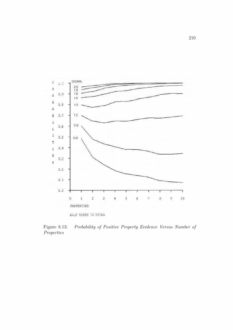
210

Figure 8.13: Probability of Positive Property Evidence Versus Number ofProperties

211

tion to ASSEMBLY identities (and surface contexts to SURFACE identities),the object types denote natural conceptual categories, and the different rela-tionship links structure the paths of evidence flow. The mathematical resultssuggest that “correct models are always invoked” if the data is well-behaved.

The “no false invocations” requirement is not easily assessed without aformal definition of “similar”, and none has been found that ensures thatfalse invocations are unlikely. So, a performance demonstration is presented,using the model base partly shown in Appendix A with the test image, andshow that the invocation process was effective and robust.

Suppose interest is in the plausibility of the trash can outer surface(“tcanoutf”) as an explanation for region 9 (see Figure 3.10). The descriptionprocess produces the following results:

DESCRIPTION VALUESmaximum surface curvature 0.091minimum surface curvature 0.0relative size 0.92absolute size 1082elongation 2.0boundary relative orientation 1.64, 1.45, 1.45, 1.73parallel boundaries 2boundary curve length 33.6, 26.7, 30.5, 28.0boundary curvature 0.058, 0.0, 0.085, 0.0

The property evidence computation is then performed, based on the fol-lowing evidence constraint (all other properties are in the description “tcan-fac”):

PROPERTY LOW PEAK HIGH WEIGHTmaximum curvature 0.058 0.078 0.098 0.5

This results in a property evidence value of 0.74 with weight 0.5. Afterinvocation converges, there are also the relationship evidence values. Nosubclasses, superclasses, subcomponents or associations were defined for thismodel, so their evidence contribution is not included. The model has adescription “tcanfac” that shares properties of the trash can inner surface(“tcaninf”) except for its convexity or concavity, and its evidence value is0.66 with a weight of 5.3. The supercomponent evidence value is 0.38 because“tcanoutf” belongs to the trash can ASSEMBLY. The maximum of the other

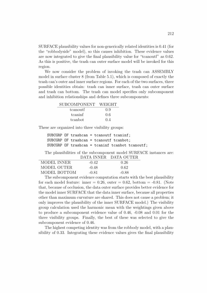
212

SURFACE plausibility values for non-generically related identities is 0.41 (forthe “robbodyside” model), so this causes inhibition. These evidence valuesare now integrated to give the final plausibility value for “tcanoutf” as 0.62.As this is positive, the trash can outer surface model will be invoked for thisregion.

We now consider the problem of invoking the trash can ASSEMBLYmodel in surface cluster 8 (from Table 5.1), which is composed of exactly thetrash can’s outer and inner surface regions. For each of the two surfaces, threepossible identities obtain: trash can inner surface, trash can outer surfaceand trash can bottom. The trash can model specifies only subcomponentand inhibition relationships and defines three subcomponents:

SUBCOMPONENT WEIGHTtcanoutf 0.9tcaninf 0.6tcanbot 0.4

These are organized into three visibility groups:

SUBCGRP OF trashcan = tcanoutf tcaninf;

SUBCGRP OF trashcan = tcanoutf tcanbot;

SUBCGRP OF trashcan = tcaninf tcanbot tcanoutf;

The plausibilities of the subcomponent model SURFACE instances are:DATA INNER DATA OUTER

MODEL INNER -0.42 0.26MODEL OUTER -0.48 0.62MODEL BOTTOM -0.81 -0.88

The subcomponent evidence computation starts with the best plausibilityfor each model feature: inner = 0.26, outer = 0.62, bottom = -0.81. (Notethat, because of occlusion, the data outer surface provides better evidence forthe model inner SURFACE that the data inner surface, because all propertiesother than maximum curvature are shared. This does not cause a problem; itonly improves the plausibility of the inner SURFACE model.) The visibilitygroup calculation used the harmonic mean with the weightings given aboveto produce a subcomponent evidence value of 0.46, -0.08 and 0.01 for thethree visibility groups. Finally, the best of these was selected to give thesubcomponent evidence of 0.46.

The highest competing identity was from the robbody model, with a plau-sibility of 0.33. Integrating these evidence values gives the final plausibility

213

for the trash can as 0.38, which was the supercomponent plausibility used inthe first example.

Because there are far too many plausibility and evidence values to de-scribe the whole network, even for this modest model base (16 ASSEMBLYs,25 SURFACEs, and 24 generic descriptions: 22 for SURFACEs and 2 forASSEMBLYs), we next present a photograph of the network to illustrate thegeneral character of the computation, and then look at the invoked modelinstances in more detail. Figure 8.14 shows all model instance nodes of thenetwork in its converged state. In the large region at the upper left of thepicture (with the textured appearance) each small grey colored rectangle rep-resents one model instance. The brightness of the box encodes its plausibility,from black (−1.0) to white (+1.0). The model instances are represented in atwo dimensional grid, indexed by the image features horizontally from left-to-right with surfaces first and then the surface clusters. The vertical indexlists the model features from top to bottom, with model SURFACEs andthen ASSEMBLYs. The two large black areas on the upper right and lowerleft arise from type incompatibility (model SURFACEs with surface clusterson the upper right and ASSEMBLYs with image surfaces on the lower left).The cover jacket of the book shows the results of the network more clearly,by encoding the plausibility from blue (−1.0) to red (+1.0).

Several interesting features can be seen immediately. First, there is astrong horizontal grouping of black and white boxes near the middle of theupper left surface pairing nodes. These are for the generic description evi-dence types, such as planar, positive cylinder, etc. As they are defined byonly a few properties, they achieve strong positive or negative plausibilities.The specific model SURFACEs are above, and other generic SURFACE fea-tures are below these. Only the specific model SURFACEs can be invoked,and there are only a few bright-grey to white nodes with a plausibility thatis high enough for this, whereas there are many darker grey low plausibilitynodes (more details below).

A similar pattern is seen in the ASSEMBLY nodes on the lower right,except for a large brightish region on the right side, with many potentiallyinvokable model instances. This bright region occurs because: (1) thereare several nested surface clusters that all contain much of the robot and(2) a surface cluster containing most of an object generally acquires a highplausibility for the whole object. This led to the explicit disabling of modelinstance nodes after verification, as described previously.

214

Figure 8.14: Model Instance Node Summary after Convergence

215

All invocations for this image are summarized in Tables 8.1 and 8.2 (sur-face clusters are listed in Table 5.1 and image regions are shown in Figure3.10). As commented above, successful invocations in one context mask invo-cations in larger containing contexts. Further, generic models are not invoked– only the object-specific models. Hence, not all positive final plausibilitiesfrom Figure 8.14 cause invocation.

ASSEMBLY invocation is selective with 18 invocations of a possible 288(16 ASSEMBLY models in 18 surface cluster contexts). Of these, all appro-priate invocations occur, and nine are in the smallest correct context and oneis in a larger context. Of the others, three are justified by close similaritywith the actual model (note 1 in the table) and five are unjustified (notes 2and 3).

SURFACE model invocation results are similar, with 21 invocations outof 475 possible (25 SURFACE models in 19 surface contexts). Of these, tenwere correct, five are justifiably incorrect because of similarity (note 1) andsix are inappropriate invocations (notes 2 and 3).

Clearly, for this image, the invocation process works well. The chief causesfor improper invocation were:

1. combinatorial surface cluster formation, resulting in similar but notdirectly related contexts which are thus not inhibited by the correctcontext, and

2. superficial similarity between features.

Possible solutions to these problems are:

• improving the depth merged surface cluster formation process and

• increasing the number of object properties.

8.4 Related Work

There is little work on model invocation in the context of three dimensionalvision. The most common technique is comparing all models to the data andis useful only when few possibilities exist.

A second level used a few easily measured object (or image) propertiesto select a subset of potential models for complete matching. Roberts [139]used configurations of approved polygons in the line image to index directly

216

Table 8.1: Invoked ASSEMBLY Model Hypotheses

SURFACE INVOCATION

MODEL CLUSTER PLAUSIBILITY STATUS NOTES

robshldbd 3 0.50 E

robshldsobj 5 0.45 E

robshldsobj 2 0.44 I 2

robshldsobj 11 0.44 I 2

robshould 11 0.39 E

trashcan 8 0.38 E

robbody 12 0.33 I 1

robbody 13 0.33 I 1

robbody 8 0.33 I 1

robbody 15 0.33 L

lowerarm 7 0.29 E

link 15 0.15 E

robot 14 0.14 I 3

robot 15 0.14 E

link 17 0.11 I 3

armasm 13 0.09 E

upperarm 9 0.05 E

robot 17 0.02 I 3

STATUSE invocation in exact contextL invocation in larger than necessary contextI invalid invocation

NOTES1 because true model is very similar2 ASSEMBLY with single SURFACE has poor discrimination3 not large enough context to contain all components

217

Table 8.2: Invoked SURFACE Model Hypotheses

SURFACE INVOCATION

MODEL REGION PLAUSIBILITY STATUS NOTES

robshldend 26 0.76 C

tcanoutf 9 0.61 C

robbodyside 9 0.41 I 1

robshoulds 29 0.40 C

robshoulds 27 0.40 I 3

ledgea 18 0.36 C

lendb 31 0.27 C

tcaninf 9 0.26 I 1

ledgeb 18 0.25 I 1

robshould1 16 0.21 I 1

robshould2 16 0.21 C

lsidea 12 0.20 I 1

lsideb 12 0.20 C

robbodyside 8 0.11 C

robshould1 12 0.10 I 3

robshould2 12 0.10 I 3

uside 19,22 0.07 C

uedgeb 19,22 0.07 I 2

lsidea 19,22 0.04 I 2

lsideb 19,22 0.04 I 2

uends 25 0.02 C

STATUSC correct invocationI invalid invocation

NOTES1 because of similarity to the correct model2 because the obscured correct model did not inhibit3 because of some shared characteristics with the model

218

models according to viewpoint. Nevatia and Binford [121] used an indexingscheme that compared the number of generalized cylinders connecting at thetwo ends of a distinguished cylinder.

Object properties have often been used to discriminate between potentialobjects in the domain using tabular and decision-tree techniques. Examplesinclude the early SRI work (e.g. [19, 156, 157]), which recognized objectsin office scenes using constraints that held between objects. This work didnot distinguish invocation from verification, and was successful because themodel bases were small, the domain simple and the objects easily discrim-inable. If model bases are large, then there are likely to be many objects withsimilar properties. Further, data errors and occlusion will make the choiceof initial index property difficult, or require vast duplication of index links.

Bolles et al. [35] implemented a powerful method for practical indexing,in their local feature focus method (for use in a two dimensional silhouetteindustrial domain). The method used key features (e.g. holes and corners) asthe primary indices (focus features), which were then supported by locatingsecondary features at given distances from the first.

Key properties are clearly needed for this task, so these were good ad-vances. However, property-based discrimination methods are sensitive toproperty estimation errors. Moreover, there are other classes of evidenceand object relationships. Property-based indexing often makes subfeaturesunusable because of their being too complex to calculate everywhere or tooobject specific. Alternately, the properties are too simple and invoke every-where and do not properly account for commonality of substructures.

When it comes to sophisticated three dimensional vision, Marr stated:

“Recognition involves two things: a collection of stored 3-D modeldescriptions, and various indexes into the collection that allow anewly derived description to be associated with a description inthe collection.” ([112], page 318)

He advocated a structured object model base linked and indexed on threetypes of links: the specificity, adjunct and parent indices, which correspondto the subclass, subcomponent and supercomponent link types used here. Heassumed that the image structures are well described and that model invo-cation is based on searching the model base using constraints on the relativesizes, shapes and orientations of the object axes. Recognized structures leadto new possibilities by following the indices. The ACRONYM system [42]implemented a similar notion.

219

Direct indexing will work for the highest levels of invocation, assumingperfect data from perfectly formed objects. However, it is probably inade-quate for more realistic situations. Further, there remains the problem oflocating the point from which to start the search from, particularly in a largemodel base.

Arbib [9] also proposed an invocation process that takes place in a schematiccontext. In his view, schemata have three components:

i. Input-matching routines which test for evidence that thatwhich the schema represents is indeed present in the envi-ronment.

ii. Action routines – whose parameters may be tuned by parameter-fitting in the input-matching routines.

iii. Competition and cooperation routines which, for example,use context (activation levels and spatial relations of otherschemas) to lower or raise the schema’s activation level.

His point (i) requires each schema to be an active matching process, butis similar, in principle, to the evidence accumulation process discussed here.His point (ii) corresponds to the hypothesis construction and verificationprocesses (Chapters 9 and 10) and point (iii) corresponds closely to the inhi-bition and relation evidence types used here. His schema invocation processwas not defined in detail and considered mainly the highest levels of descrip-tion (e.g. of objects) and only weakly on the types of visual evidence or theactual invocation computation.

Hoffman and Jain [90] described an evidence-based object recognitionprocess that is similar to the one described in this chapter. Starting froma set of surface patches segmented from range data, they estimated a setof unary and binary properties. Evidence conditions were formulated asconjunctions of property requirements. The degree to which an evidencecondition supported or contradicted each model was also specified. When anunknown object was observed, a similarity measure was computed for eachmodel. This approach can use object-specific evidence conditions, leading tomore precise identification, but at the cost of evaluating the conditions forall objects. Good results were demonstrated with a modest model-base.

Binford et al. [30] also described a similar (though probability based)invocation approach. The scheme uses a “Bayesian network”, where proba-bilities accumulate from subcomponent relationships and originate from the

220

likelihood that an observed two dimensional image feature is the projectionof a three dimensional scene feature. Reliability is enhanced by only using“quasi-invariant” features (i.e. those nearly constant over a large range ofviewing positions), such as the fixed relative orientation between two axes.The network formulation used alternating layers of object and relative place-ment relationships (“joints”). Subcomponent a priori distributions were gen-erated heuristically from occurrences in the model base.

There are obvious links between the network approach described hereand the connectionist approach. In the latter, the domain knowledge isimplicit in the weighted interconnections between simple identical processingunits, which represents the interobject relationships. These machines canconverge to a fixed output state for a given input state, and can learn networkconnection weights (e.g. [92, 88, 2]). Many of the computations proposed forinvocation can probably be implemented using such devices.

Hinton proposed and evaluated ([87, 89]) a connectionist model of invo-cation that assigns a reference frame as well as invoking the model. Themodel uses connections between retinotopic feature units, orientation map-ping units, object feature (subcomponent) units and object units. This modelrequires duplicated connections for each visible orientation, but expressesthem through a uniform mapping method. Consistent patterns of activitybetween the model and data features reinforce the activation of the mappingand model units. The model was proposed only for two dimensional patterns(letters) and required many heuristics for weight selection and convergence.

Feldman and Ballard [64] proposed a connectionist model indexing schemeusing spatial coherence (coincidence) of properties to gate integration of ev-idence. This helps overcome inappropriate invocation due to coincidentallyrelated features in separate parts of the image. The properties used in theirexample are simple discriminators: “circle, baby-blue and fairly-fast” for afrisbee.

This proposal did not have a rich representation of the types of knowl-edge useful for invocation nor the integration of different types of evidence,but did propose a detailed computational model for the elements and theirconnections.

Feldman [65] later refined this model. It starts with spatially co-locatedconjunctions of pairs of properties connected in parallel with the featureplane (descriptions of image properties). Complete objects are activatedfor the whole image based on conjunctions of activations of these spatiallycoincident pairs. The advantage of complete image activation is that with this

221

method it is not necessary to connect new objects in each image location. Thedisadvantage is in increased likelihood of spurious invocations arising fromcross-talk (i.e. unrelated, spatially separated features invoking the model).Top-down priming of the model holds when other knowledge (e.g. worldknowledge) is available. Structured objects are represented by linkage to thesubcomponents in the distinct object viewpoints. Multiple instances of theobjects use “instance” nodes, but little information is given to suggest howthe whole image model can activate separate instances.

These approaches are similar to those of this chapter: direct property ev-idence triggers structurally decomposed objects seen from given viewpoints.The network formulation for invocation proposed here has a parallel struc-ture for two reasons: (1) the need for fast retrieval and (2) it is a convenientformalism for expressing the computational relationships between evidencetypes.

A key difference between the connectionist work reviewed above and thework described in this book is the use of dedicated network structures, asspecified by the evidence type’s constraints, etc. There is also an implemen-tation difference, in that many of the connectionist networks express theirresults as states or configurations of activity of the network, rather than asthe activity at a single node, which is the approach here.

Other Potential Techniques

There has been little Artificial Intelligence research done that treatedmodel invocation as a specific issue. Work (e.g. [116, 144]) has focusedmore on the contents and use of models or schemas than on how a schemais selected.

The NETL formalism of Fahlman ([58, 59]) is a general indexing approachto invocation. This approach creates a large net-like database, with gener-alization/specialization type links. One function of this structure is to allowfast parallel search for concepts based on intersections of properties. Forexample, an elephant node is invoked by intersection of the “large”, “grey”and “mammal” properties. The accessing is done by way of passing mark-ers about the network (implemented in parallel), which is a discrete form ofevidence passing. The few links used in this approach make it difficult toimplement suggestiveness, as all propagated values must be based on certainproperties.

222

General pattern recognition/classification techniques are also of some usein suggesting potential models. A multi-variate classifier (e.g. [56]) couldbe used to assign initial direct evidence plausibility to structures based onobserved evidence. Unfortunately, this mechanism works well with propertyevidence, but not with integrating evidence from other sources, such as fromsubcomponent or generic relationships. Further, it is hard to provide the apriori occurrence and property statistics needed for the better classifiers.

The relaxation-based vision processes are also similar to the plausibilitycomputation. Each image structure has a set of possible labels that mustbe consistent with the input data and related structure labels. Applicationshave tended to use the process for either image modification [141], pixel clas-sification [82], structure detection, or discrete consistency maintenance [162].Most of the applications modify the input data to force interpretations thatare consistent with some criterion rather than to suggest interpretations thatare verified in another manner. Unfortunately, invocation must allow multi-ple labels (generics) and has a non-linear and non-probabilistic formulationthat makes it difficult to apply previous results about relaxation computa-tions.

8.5 Discussion

The purpose of invocation is to reduce the computation involved in the model-to-data matching process. This has been partially achieved by basing invoca-tion on propagated plausibility values, so the computation has been reducedfrom a detailed object comparison to evidence accumulation. Unfortunately,virtually every object model still needs to be considered for each image struc-ture, albeit in a simplified manner. On the other hand, the model-to-datacomparison computation has now been simplified. As a result, it is nowamenable to large scale parallel processing.

One deficiency in this method is the absence of a justified formal criterionthat determines when to invoke a model. Invoking when the plausibility waspositive worked well in practice, but most seriously incorrect hypotheses arenear -1.0. Hence, a threshold somewhat lower than 0.0 could be considered.This might lead to each object having a different threshold.

This work leaves several open “learning” problems:

1. How is the structure of the model network created and modified?

223

2. How are the features used for invocation selected?

3. How are the property and relationship weights chosen?

Other unsolved problems include resolving the problem of multiple invo-cations within the extended surface cluster hierarchy (as discussed above),preventing data feature evidence from being used for more than one modelsubcomponent and deciding when to invoke generic models (as well as theobject-specific ones). The theory could also be extended for non-shape prop-erties (e.g. color, texture, etc.) and quantified descriptors (e.g. “larger”,“much larger”) proposed by Marr [112] as an attempt to achieving scale in-variance. Finally, though the class hierarchy and evidence computations weredefined, no significant testing of this feature was undertaken.

For each evidence computation, some natural constraints were proposedas specification criteria. But, there were never enough constraints to uniquelydetermine the computation. The hope is that the variations in algorithmsthat this allows result only in slightly different performance levels. This hasbeen partially tested using substantially different property evidence evalua-tion and evidence integration functions, without significant differences in theinvocation results.

This chapter has only concerned visual recognition, but this invocationapproach may have more general applicability. Any form of symbolic infer-ence requires accessing the correct symbol. So, the model invocation problemis also a general cognitive problem, with the following aspects:

• low level symbolic assertions are produced for the current input whetherfrom an external (e.g. raw sense data) or internal (e.g. self-monitoring)source,

• higher level concepts/symbols tend to be semi-distinctly characteriz-able based on “configurations” of lower level symbolic descriptions,

• there are many potential higher level symbols, but only a small subsetshould be selected for closer consideration when matching a symbol,

• the importance of a particular concept in invoking another is dependenton many factors, including structure, generics, experience and context,and

• symbols “recognized” at one description level (either primitive or throughmatching) become usable for the invocation of more complex symbols.

224

Examples of this in a non-vision context might be something like an invo-cation of a Schankian fast-food restaurant schema [144] or recognizing wordsin speech.

Final Comments

This chapter formalized the associative basis of a model invocation pro-cess with the major elements as object types, property evidence inputs andassociative links based on generic and component relations. The theory wasbased on sets of constraints describing how different evidence affects plausi-bility, and the use of surfaces and surface clusters as the contexts in whichto accumulate evidence.

Chapter 9

Hypothesis Construction

At this point the recognition process has isolated a set of data, describedits features and invoked a model as its potential identity. To claim thatthe object is genuinely recognized requires the pairing of model features toimage data. Without these correspondences object recognition is only sug-gestive – like saying a collection of gears and springs is a watch. Hence, thehypothesis construction process has the goal of fully instantiating correctlyinvoked models, estimating object position and accounting for the appear-ance of the object, including occlusion. These tasks are the first stage insubstantiating the existence and identity of the object, as described in thischapter.

The chapter also describes some more recent work that uses a value-propagating network for geometric reasoning.

9.1 Thoughts on Hypothesis Construction

The hypothesis construction process described below attempts to find evi-dence for all model features. This is somewhat controversial and it is worth-while to briefly discuss the motivations for this decision.

If we are working in a restricted domain (such as on an industrial assem-bly line) the numbers and types of objects in the scene are usually limited.Here, many details would be object-specific, and a goal-directed argumentsuggests that only the key differentiating features need be found. Whenthe domain is sufficiently restricted, specific features will be unique signi-fiers. However, this would not be an appropriate strategy for a general vision

225

226

system because, without additional descriptions or non-visual knowledge ofthe restricted domain, it would not ordinarily be possible to reach the stagewhere only a few identities were under consideration.

However, identifying individuals or subclasses requires finer details (e.g.distinguishing between two people, or even between two “identical” twins).Many individual objects differ only slightly or share identical features. Con-sider how often one recognizes a facial feature or a smile of a friend in the faceof a complete stranger. Though the stranger is unique through the configu-ration of his/her features, some details are held in common with the friend.If recognition were predicated on only a few features, which may sometimesbe sufficient for unique identification in a limited domain, then we would becontinually misrecognizing objects. While only a few may be necessary formodel invocation, many others are necessary for confirmation.

These problems suggest that the hypothesis construction process shouldtry to find direct image evidence for all model features.

On the other hand, partial evidence is often sufficient. We usually haveno trouble identifying a friend even when a mustache has been shaved off,and often do not even notice that there is a change, let alone know what thechange is. Or we can often recognize them, having seen only a portion oftheir face.

Moreover, finding evidence for all features is usually impossible, as reso-lution changes might make the information too large or too small to directlydetect, and occlusion will hide some of it.

Yet, we tend to expect recognition to be perfect. So, on idealistic grounds,a general vision system should acquire as much information as possible. Thisis also supported by the usual role of a general vision system – that it shouldbe a largely autonomous, data-driven analysis system, providing environmen-tal descriptions to a higher-level action module, which may then instigateadditional goal-directed visual analysis.

In summary, our desire for full model instantiation derives from:

• a philosophical requirement – that true image understanding requiresconsistent interpretation of all visible features relative to a model andcontingent explanation of missing features,

• an environmental requirement – that many details are needed to distin-guish similar objects, especially as objects share common features andsome details will be absent for environmental reasons (e.g. occlusion),and

227

• a practical requirement – that objects should be recognized to the de-gree they need to be distinguished.

Why Use Surfaces as Evidence

What is desired is image evidence that supports the existence of eachmodel feature. In edge-based recognition systems, an image edge was thekey evidence for a model feature, because surface orientation discontinuityboundaries were observed as edges. This was even more important in polyhe-dral domains (without reflectance boundaries), where extremal boundarieswere also orientation discontinuity boundaries. Unfortunately, more natu-rally shaped and colored objects led to a veritable plethora of problems:there were fewer traditional orientation edges, extremal boundaries no longercorresponded to orientation discontinuities and reflectance and illuminationvariations created new edges. So, these made the search for simple and di-rectly corresponding edge evidence much more difficult.

Two of the advantages of using surfaces given in Chapter 3 are mentionedhere again:

• using surfaces as the primary representational unit of both the raw dataand the object model makes the transformation distance between thetwo almost non-existent, and

• the interpretation of a surface data unit is unambiguous (unlike imageedges, which may correspond to a variety of scene phenomena).

With surface representations, it is again possible to find image evidencethat directly matches with model features. Assuming that there is a con-sistent segmentation regimen for both the surface image and model SUR-FACEs, the model feature instantiation problem can be reduced to findingwhich model SURFACE corresponds to each data surface.

Finding all model features first requires understanding how three dimen-sional objects appear in images – to locate image evidence for oriented modelinstances. Here the recognition process must understand, or at least be ableto predict how a surface patch’s appearance varies with changes in the sur-face’s position relative to the viewer. The segmentation process attempts toproduce surface patches with a uniform curvature characterization, so it iseasy to approximate the visible shape to first-order, given the model patch

228

and its relative position. Also, given recent advances in computer graphics,it is possible to deduce the visibility status of most surface patches.

Another result of using the surface segmentation is a discrete symbolicpartitioning of the complete object surface. This simplifies the surface match-ing computation tremendously. An infinitesimal element of a surface couldhave many possible identities and this shows up in practice as the need torotate incrementally and shift surfaces when matching (e.g. [96, 135]). Asegmented surface immediately simplifies the matching by choosing a higherlevel structure for comparison. Topology further decreases the amount ofmatching as adjacent model SURFACEs must pair with adjacent data sur-faces, reducing the problem to subgraph isomorphism. If the invocationprocess gives strong suggestions to the identity of the various surfaces, thencombinatorial matching is almost completely unnecessary.

9.2 Deducing Object Position

Part of competent object recognition is knowing where an object is – henceits three dimensional location and orientation must be determined. Thisinformation is also needed internally, as identity verification requires findingthat all visible object features are correctly placed. Moreover, an estimate ofan object’s position enables prediction of image locations for missing features.

Invocation suggests a few model-to-data feature (e.g. surface) correspon-dences to form an initial “island of stability”. From this, the reference frameof the object relative to the viewer can be deduced by analyzing the geometricrelationships between the features. For example, a single surface correspon-dence constrains the object to a single rotational degree-of-freedom abouta nominal surface normal (assuming that the model and data normals canbe paired). A second rotation axis, whether from a second surface or froman axis of curvature on the first surface, usually completely constrains theobject’s orientation (though possibly up to a mirror image).

9.2.1 Geometric Reasoning

Recently, Orr [126] analyzed several prominent three dimensional scene anal-ysis systems, including the IMAGINE I system described here, and con-cluded that five generic functions provided the geometric reasoning neededfor most computer vision tasks. The functions were:

229

LOCATE – producing position estimates from model-to-data feature cor-respondences,

PREDICT – predicting a data feature for a given model feature, given anestimate of the object’s position,

MERGE – integrating two position estimates to produce a better estimate,or to signal inconsistency between the estimates,

TRANSFORM – expressing a position in another reference frame and

INVERSE – inverting the transformation between two reference frames.

Central to these functions was a position data type, that represented therotation and translation between two geometric reference frames. This re-lationship may be exact (as in a model), complete but inexact (as whenaccounting for measurement uncertainty), or partial (as represented by, forexample, an underdetermined rotation constraint).

At the time of the research undertaken here, two of the best approachesto representing position estimates were based on either an explicit completeposition, perhaps with some error estimates (i.e. from a least-squared errortechnique, such as Faugeras and Hebert [63]) or by parameter ranges, linkedto algebraic inequality constraints over the parameters (as in the ACRONYMsystem [42]).

The first approach integrated a set of uniform data (e.g. model-to-datavector pairings) to give a single-valued estimate, but at some computationalcost. On the other hand, ACRONYM’s advantage was that it could easily in-tegrate new evidence by adding new constraints, the range of possible valueswas made explicit and inconsistency was detectable when parameter rangesbecame non-existent. Its disadvantage was that the current estimate for aparameter was implicit in the set of constraints and could only be obtainedexplicitly by substantial algebraic constraint manipulation of non-linear in-equalities, which result only in a range of values with no measure of “best”.

More recent work by Durrant-Whyte [57] represented position estimatesstatistically, computing the transformations of positions by a compositiontechnique. This has the advantage of propagating uncertainties conciselyand gives a “best” estimate, but does not easily provide the means to de-termine when inconsistency occurs (other than low probability). Further,

230

approximations are needed when the reference frame transformations them-selves involve uncertainty, or when uncertainty is other than statistical (e.g.a degree-of-freedom about a joint axis).

The techniques used in IMAGINE I are now described, and related tothe five function primitives described above.

Each individual parameter estimate is expected to have some error, soit is represented by a range of values. (The initial size of the range wasbased on experience with parameter estimation.) An object’s position isthen represented by a six dimensional parameter volume, within which thetrue parameter vector should lie. Thus, the position representation is asimplified, explicit version of that used by ACRONYM (but less precise,because constraint boundaries are now planes perpendicular to the coordinateaxes). This leads to more efficient use, while still representing error rangesand detecting inconsistency.

Integrating parameter estimates (i.e. MERGE) is done by intersecting theindividual parameter volumes. All the six dimensional parameter volumesare “rectangular solids” with all “faces” parallel, so that the intersection iseasily calculated and results in a similar solid. Because the true value iscontained in each individual volume, it must also lie in the intersection. Theeffect of multiple estimates is to refine the tolerance zone by progressivelyintersecting off portions of the parameter volume, while still tolerating errors.If a final single estimate is needed, the average of each pair of limits is used.

As described so far, the transformation of coordinate reference systems(TRANSFORM) has been done by multiplication of the homogeneous coor-dinate matrices representing the transforms. Since we are now using a pa-rameter estimate range, the transformation computation must be modified.In the most general case, each transformation would have its own range, but,as implemented here, only the transformation from the camera coordinatesystem to the object global reference frame is allowed statistical variations.(Although, transformations may have parameterized degrees-of-freedom – seeChapter 7.) These variations propagate through the calculation of the globalor image locations for any feature specified in any level of reference frame.The variation affects two calculations:

1. how to calculate a combined transformation given that one transfor-mation is a range, and

2. how to calculate the range of positions for a point given a transforma-tion range.

231

The technique used for both of these problems is similar, and is only anapproximation to a complete solution:

1. For a subset of values in the parameter range,

(a) Calculate a transformation

(b) Transform the second parameter vector (or point)

2. Bound the set of transformed vectors (or points).

This process is illustrated in Figure 9.1. In part (a), a two dimensionalparameter range with the subset of points is designated. In part (b), theoriginal range is rotated to a new range, and part (c) shows the parameterbounds for the new range.

The figure illustrates one problem with the method – parameter boundsare aligned parallel with the coordinate axes, so that the parameter vol-ume (actually six dimensional) increases with each transformation. A secondproblem is that the rotation parameter space is not rigid in this coordinatesystem, so that the shape of the parameter space can change greatly. If itexpands in a direction not parallel with a coordinate axis, the combinationof the first problem with this one can result in a greatly expanded parameterspace. Further, the transformation is not unique, as zero slant allows anytilt, so any transformations that include this can grow quickly.

One general problem with the method is that consistent data does notvary the parameter bounds much, so that intersecting several estimates doesnot always tighten the bounding greatly. Hence, there is still a problemwith getting a “best” estimate from the range. Another problem with thegeneral case is that each model variable increases the dimensionality of theparameter space, requiring increased computation and compounding bound-ing problems.

The conclusion is that this simplified method of representing and manip-ulating parameter estimates is not adequate, which led to the work by Fisherand Orr [74] described in Section 9.2.4.

The INVERSE function occurs in two forms. Inverting an exact transfor-mation (represented by a homogeneous coordinate matrix) is simply matrixinversion. Inverting an estimate range is given by bounding the inversions ofa subset of the original range (similar to TRANSFORM).

The PREDICT function uses either an exact transformation from themodel or the mean value of a data-derived parameter range to predict either

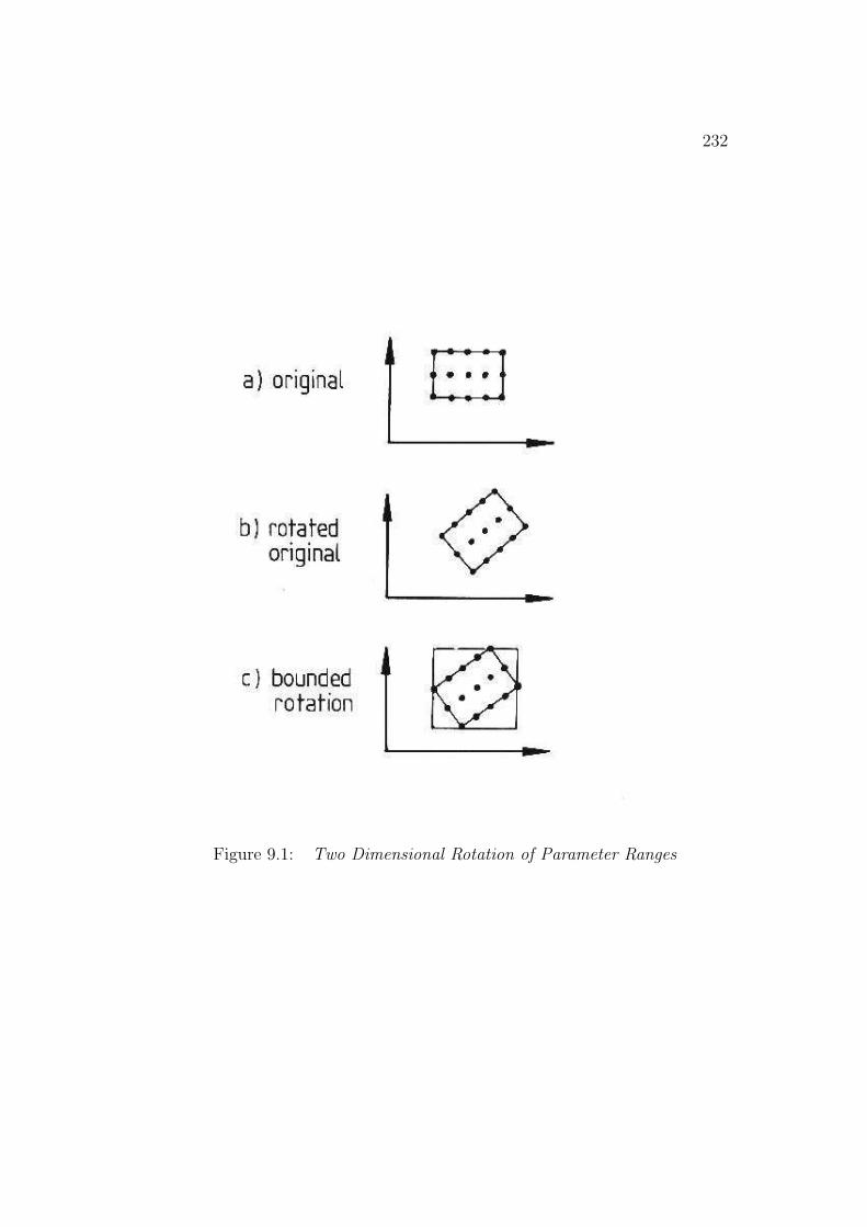
232

Figure 9.1: Two Dimensional Rotation of Parameter Ranges

233

three dimensional vector directions, three dimensional points or two dimen-sional points (by projection of the three dimensional points).

The LOCATE function is specific to the data and model feature pairings,and is described in more detail in the next two sections.

9.2.2 Estimating Individual Surface Reference Frames

Estimating Surface Rotation

A SURFACE’s spatial position is represented by the transformation from thecamera coordinate frame to that of the SURFACE. Several constraints areavailable to help deduce the transformation.

Fisher [66] showed how the transformation could be deduced using thetwo dimensional boundary shape. Estimation of the orientation parameters(rotation, slant and tilt) used the cross-section width as a function of theimage angle, which deforms in a characterizable way.

In the research presented here, surface normals are directly available. Ifa planar data patch is paired with a model patch, their normal vectors mustbe parallel so only one rotational degree-of-freedom needs to be resolved.The final rotation degree-of-freedom is estimated by correlating the angularcross-section width as a function of rotation angle. Figure 9.2 illustrates this.For non-planar surfaces, an approximate solution is obtained by using thenormals at the centroids of the surfaces. A more complete solution using thecurvature axis is presented below.

The complete method is:

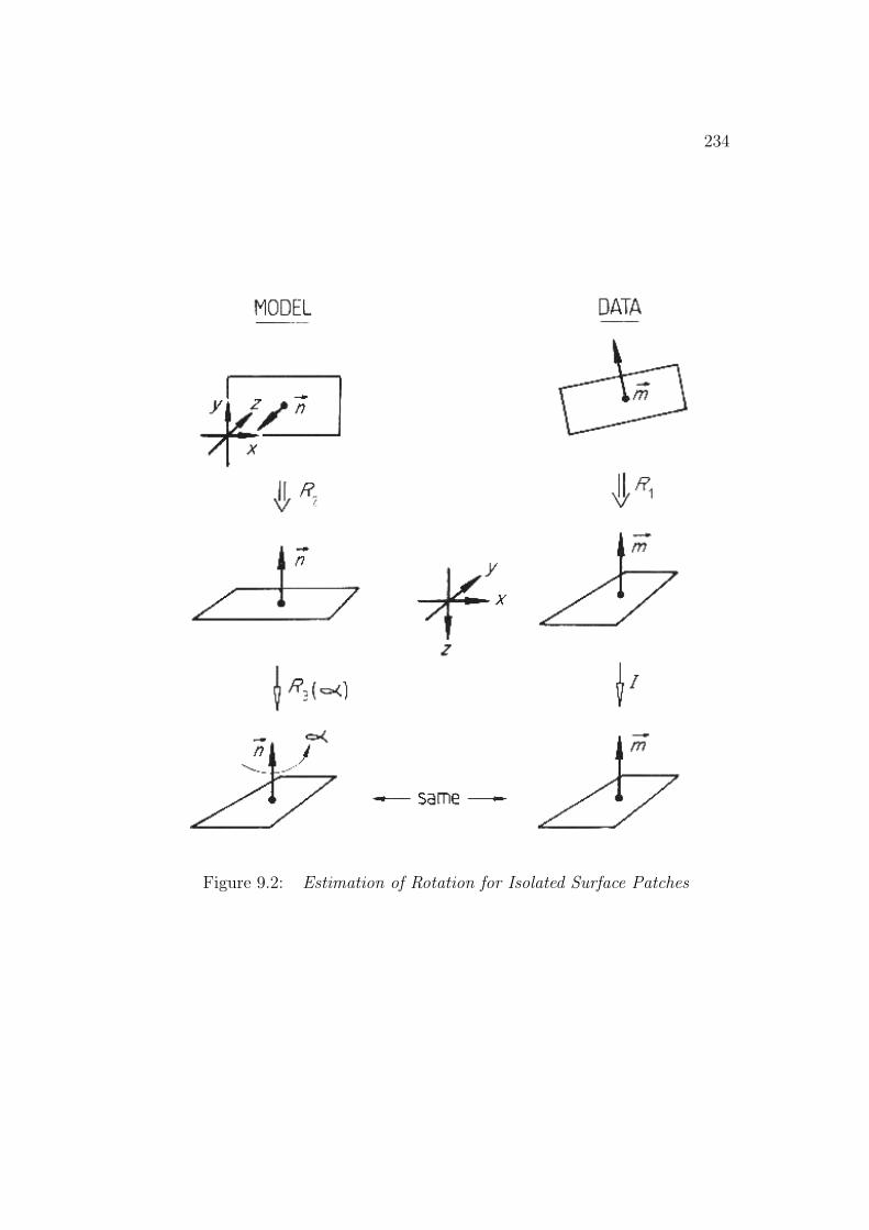
234

Figure 9.2: Estimation of Rotation for Isolated Surface Patches

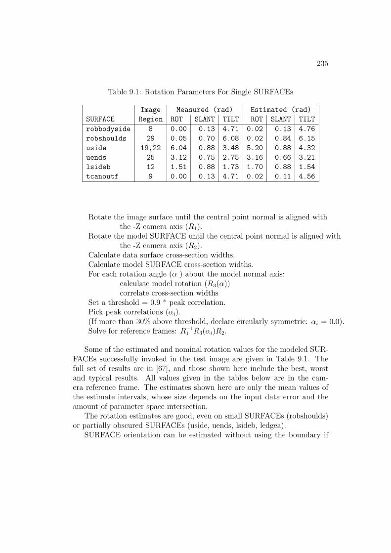
235

Table 9.1: Rotation Parameters For Single SURFACEs

Image Measured (rad) Estimated (rad)

SURFACE Region ROT SLANT TILT ROT SLANT TILT

robbodyside 8 0.00 0.13 4.71 0.02 0.13 4.76

robshoulds 29 0.05 0.70 6.08 0.02 0.84 6.15

uside 19,22 6.04 0.88 3.48 5.20 0.88 4.32

uends 25 3.12 0.75 2.75 3.16 0.66 3.21

lsideb 12 1.51 0.88 1.73 1.70 0.88 1.54

tcanoutf 9 0.00 0.13 4.71 0.02 0.11 4.56

Rotate the image surface until the central point normal is aligned withthe -Z camera axis (R1).

Rotate the model SURFACE until the central point normal is aligned withthe -Z camera axis (R2).

Calculate data surface cross-section widths.Calculate model SURFACE cross-section widths.For each rotation angle (α ) about the model normal axis:

calculate model rotation (R3(α))correlate cross-section widths

Set a threshold = 0.9 * peak correlation.Pick peak correlations (αi).(If more than 30% above threshold, declare circularly symmetric: αi = 0.0).Solve for reference frames: R−1

1 R3(αi)R2.

Some of the estimated and nominal rotation values for the modeled SUR-FACEs successfully invoked in the test image are given in Table 9.1. Thefull set of results are in [67], and those shown here include the best, worstand typical results. All values given in the tables below are in the cam-era reference frame. The estimates shown here are only the mean values ofthe estimate intervals, whose size depends on the input data error and theamount of parameter space intersection.

The rotation estimates are good, even on small SURFACEs (robshoulds)or partially obscured SURFACEs (uside, uends, lsideb, ledgea).

SURFACE orientation can be estimated without using the boundary if

236

Figure 9.3: Rotation Estimation from Normal and Curvature Axis

there is significant surface curvature in one direction. Here, the three di-mensional orientation of the major curvature axis constrains the remainingangular degree-of-freedom to two possible orientations. The transformationfrom the model normal and curvature axis vectors to those of the data givesthe orientation estimate. Data errors complicate the calculation, which isdescribed in detail in Section 9.2.3. Figure 9.3 illustrates the process of ro-tation estimation using the normal and curvature axis. Table 9.2 lists theresults for this case.

Table 9.2: Rotations for Single SURFACEs Using the Curvature Axis

Image Measured (rad) Estimated (rad)

SURFACE Region ROT SLANT TILT ROT SLANT TILT

robbodyside 8 0.00 0.13 4.71 6.28 0.13 4.77

robshoulds 29 0.05 0.70 6.08 0.10 0.83 6.07

uends 25 3.12 0.75 2.75 3.12 0.66 3.24

tcanoutf 9 0.00 0.13 4.71 0.01 0.18 4.61

237

Table 9.3: Combined Rotation Parameters For Single SURFACEs

Image Measured (rad) Estimated (rad)

SURFACE Region ROT SLANT TILT ROT SLANT TILT

robbodyside 8 0.00 0.13 4.71 0.01 0.13 4.76

robshoulds 29 0.05 0.70 6.08 0.02 0.83 6.15

uends 25 3.12 0.75 2.75 3.16 0.66 3.21

tcanoutf 9 0.00 0.13 4.71 0.01 0.18 4.56

Table 9.3 shows the results obtained by integrating the above results withthose from Table 9.1 (by parameter space intersection). As the curvaturebased estimation process gives nearly the same results as the boundary basedprocess, the intersection hardly improves the results. This suggests that theinitial estimation techniques are both generally accurate.

Estimating SURFACE Translations

Given the rotations, the translations are estimated. Fisher [66] estimatedthese directly from the boundary data. Depth was estimated by comparingmodel and data areas and cross-section widths. The three dimensional trans-lation was estimated using the two dimensional translation that best fittedthe data and then inverting the projection relationship using the estimateddepth.

Here, depth estimates are directly available, and the xy translation isestimated by relating the rotated model SURFACE centroid to the two di-mensional image centroid and inverting the projection relationship. Typicalestimated and nominal translation values for the modeled SURFACEs suc-cessfully invoked in the test image are given in Table 9.4.

The translation estimates are reasonable, though not as accurate as therotation estimates. This is true even though SURFACEs lsideb, ledgea anduside were substantially obscured. For the unobscured SURFACEs, the av-erage translation error for the test image is (-6.0,1.6,-1.6), and is believed toarise from errors in estimating the camera coordinate system. Other sourcesof error include measurement error (estimated as 1.0 cm and 0.1 radian),image quantization (estimated as 0.6 cm at 5m and 0.002 radian) and errorsarising from the approximate nature of the parameter estimations. In any

238

Table 9.4: Translation Parameters For Single SURFACEs

Image Measured (cm) Estimated (cm)

SURFACE Region X Y Z X Y Z

robbodyside 8 -13.9 -32.4 565 -13.5 -35.9 562

robshoulds 29 -20.9 17.8 556 -16.2 9.8 564

uside 19,22 -21.0 13.4 585 -13.6 31.0 578

uends 25 27.2 16.6 547 35.6 16.5 551

lsideb 12 23.7 16.9 533 21.9 28.4 539

tcanoutf 9 22.3 -44.1 536 29.1 -44.2 541

case, the error is about 1.5% of the distance to the object, so the relativeposition error is small.

To illustrate the position results for the test image better, several pic-tures are shown with the SURFACEs drawn in their estimated positions ontop of the original scene. Figure 9.4 shows the robot body side SURFACE(robbodyside), the robot upper arm side SURFACE (uside) and the trashcan outer SURFACE (tcanoutf). Figure 9.5 shows the robot shoulder endSURFACE (robshldend), the robot lower arm side SURFACE (lsideb) andthe robot upper arm small end SURFACE (uends). The lower arm sideSURFACE y translation estimate is high because of occlusion.

9.2.3 Estimating ASSEMBLY Reference Frames

If a set of model vectors (e.g. surface normals) can be paired with correspond-ing data vectors, then a least-squared error estimate of the transformationcould be estimated using methods like that of Faugeras and Hebert [63].This integrates all evidence uniformly. The method described below esti-mates reference frame parameters from smaller amounts of evidence, whichis then integrated using the parameter space intersection method describedabove. The justification for this approach was that it is incremental andshows the intermediate results more clearly. It can also integrate evidencehierarchically from previously located subcomponents.

Each data surface has a normal that, given correspondence with a par-ticular model SURFACE, constrains the orientation of the ASSEMBLY to asingle rotational degree-of-freedom about the normal. A second, non-parallel,

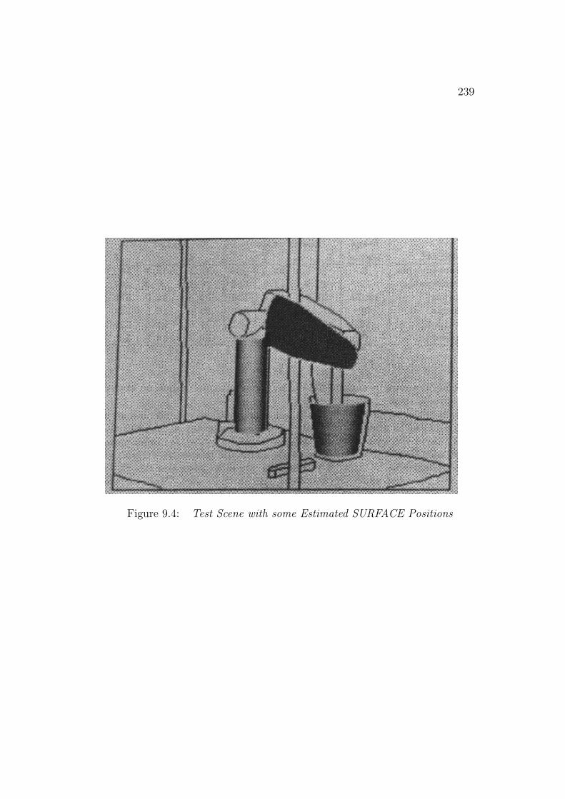
239

Figure 9.4: Test Scene with some Estimated SURFACE Positions

240

Figure 9.5: Test Scene with Other Estimated SURFACE Positions

241

Figure 9.6: Rotating Model Normals to Derive the Reference Frame

surface normal then fixes the object’s rotation. The calculation given hereis based on transforming a pair of model SURFACE normals onto a datapair. The model normals have a particular fixed angle between them. Giventhat the data normals must meet the same constraint, the rotation thattransforms the model vectors onto the data vectors can be algebraically de-termined. Figure 9.6 illustrates the relationships.

Use of surface normals is reasonable only for nearly planar surfaces. Forcylindrical or ellipsoidal surfaces, normals at the central points on the dataand model surfaces can be computed and compared, but: (1) small displace-ments of the measurement point on surfaces with moderate curvature lead tosignificant changes in orientation, and (2) occlusion makes it impossible toaccurately locate corresponding points. Fortunately, highly curved surfacesoften have a curvature axis that is more accurately estimated and is not de-pendent on precise point positions nor is it affected by occlusion. Figure 9.7

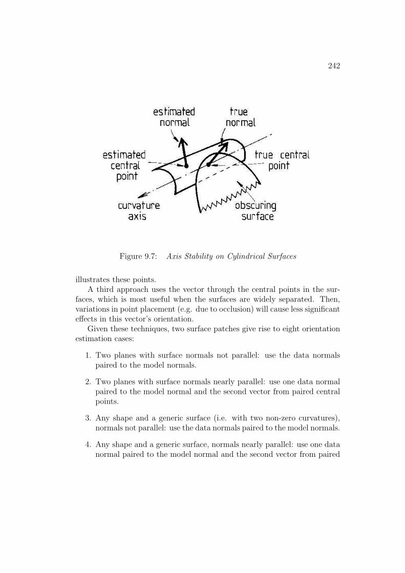
242

Figure 9.7: Axis Stability on Cylindrical Surfaces

illustrates these points.A third approach uses the vector through the central points in the sur-

faces, which is most useful when the surfaces are widely separated. Then,variations in point placement (e.g. due to occlusion) will cause less significanteffects in this vector’s orientation.

Given these techniques, two surface patches give rise to eight orientationestimation cases:

1. Two planes with surface normals not parallel: use the data normalspaired to the model normals.

2. Two planes with surface normals nearly parallel: use one data normalpaired to the model normal and the second vector from paired centralpoints.

3. Any shape and a generic surface (i.e. with two non-zero curvatures),normals not parallel: use the data normals paired to the model normals.

4. Any shape and a generic surface, normals nearly parallel: use one datanormal paired to the model normal and the second vector from paired

243

central points.

5. Plane and cylinder, cylinder axis not parallel to plane normal: usepaired plane data and model normals, paired cylinder data and modelaxes.

6. Plane and cylinder, cylinder axis nearly parallel to plane normal: usethe data normals paired to the model normals.

7. Two cylinders, axes not parallel: use data axes paired with model axes.

8. Two cylinders, axes nearly parallel: use one data axis paired to themodel axis and the second vector from paired central points.

After feature pairing, the rotation angles are estimated. Unfortunately,noise and point position errors mean that the interior angles between the pairsof vectors are only approximately the same, which makes exact algebraicsolution impossible. So, a variation on the rotation method was used. Athird pair of vectors, the cross product of each original pair, are calculatedand have the property of being at right angles to each of the original pairs:

Let:~d1, ~d2 be the data normals~m1, ~m2 be the model normals

Then, the cross products are:

~cd = ~d1 × ~d2

~cm = ~m1 × ~m2

From ~d1 and ~cd paired to ~m1 and ~cm an angular parameter estimatecan be algebraically calculated. Similarly, ~d2 and ~cd paired to ~m2 and ~cm

gives another estimate, which is then integrated using the parameter spaceintersection technique.

Fan et al. [61] used a somewhat similar paired vector reference frame esti-mation technique for larger sets of model-to-data vector pairings, except thatthey picked the single rotation estimate that minimized an error function,rather than integrated all together. This often selects a correct rotation froma set of pairings that contains a bad pairing, thus allowing object recognitionto proceed.

244

Before the rotation is estimated from a pair of surfaces, a fast compatibil-ity test is performed, which ensures that the angle between the data vectorsis similar to that between the model vectors. (This was similar to the angularpruning of Faugeras and Hebert [63]). The test is:

Let:~d1, ~d2 be the data normals~m1, ~m2 be the model normals

If:

| (~d1 ◦ ~d2) − (~m1 ◦ ~m2) |< τc (τc = 0.3)

Then, the vector pairs are compatible.

The global translation estimates come from individual surfaces and sub-structures. For surfaces, the estimates come from calculating the translationof the nominal central point of the rotated model SURFACE to the estimatedcentral point of the observed surface. Occlusion affects this calculation bycausing the image central point to not correspond to the projected modelpoint, but the errors introduced by this technique were within the level oferror caused by mis-estimating the rotational parameters. The implementedalgorithm for SURFACEs is:

Let:G be the transformation from the ASSEMBLY’s coordinate

system to that of the cameraA be the transformation from the SURFACE’s coordinate system

to that of the ASSEMBLYThen:

1. Get the estimated global rotation for that SURFACE: (GA)2. Rotate the central point (~p) of the model SURFACE: (~v1 = GA~p)3. Calculate the three dimensional location (~v2) of the image region

centroid, inverting its image coordinates using the depthvalue given in the data

4. Estimate the translation as ~v2 − ~v1

245

ASSEMBLY Reference Frame Calculation Results

The estimation of an ASSEMBLY’s reference frame is demonstrated for therobot lower arm.

As the rigidly attached hand subcomponent is not visible, it contributesno information. Each of the SURFACEs paired and transformed accordingto the above theory contributes to these estimates (in the camera coordinatesystem):

OBJECT ROT SLANT TILTlsideb & lendb MIN 3.966 1.158 4.252

MAX 0.633 0.204 3.949

lendb & ledgea MIN 3.487 1.190 4.693MAX 0.192 0.216 4.405

ledgea & lsideb MIN 3.853 1.361 4.599MAX 0.430 0.226 4.257

The rotation estimates are integrated by intersection to give the followingresult:

ROT SLANT TILTMIN 3.966 1.361 4.693MAX 0.192 0.204 3.949

and the average value is:

ROT SLANT TILT5.220 2.353 1.180

which compares well with the measured value of:

ROT SLANT TILT5.060 2.236 1.319

Translation is estimated after rotation, and starts with an estimate from

246

each individual SURFACE. These estimates are:

X Y Zlsideb MIN -1.891 -10.347 503.

MAX 57.262 48.807 592.

lendb MIN -1.206 -26.849 500.MAX 58.259 32.616 589.

ledgea MIN -1.058 -20.298 503.MAX 58.116 38.875 592.

The translation estimates are integrated by intersection to give the fol-lowing result:

X Y ZMIN -1.058 -10.347 503.MAX 57.262 32.616 589.

and the average value is:

X Y Z28.1 11.1 546.

which compares well with the measured value of:

X Y Z26.6 8.79 538.

Tables 9.5 and 9.6 summarize the results for the primitive ASSEMBLYs inthe test image whose estimates resulted from using more than one SURFACE.The other primitive ASSEMBLYs have reference frames identical to thatof the single SURFACE (rotated into the ASSEMBLY’s reference frame ifnecessary). All results are given in the camera coordinate system. Theparameter estimates are good, even though both the upper and lower armare substantially obscured.

Estimating Reference Frames from Previously Recognized Sub-components

Each previously recognized subcomponent contributes a position estimate.Suppose, the subcomponent has an estimated global reference frame Gs and

247

Table 9.5: Translation Parameters For Primitive ASSEMBLYs

Measured (cm) Estimated (cm)

ASSEMBLY X Y Z X Y Z

robshldbd -13.9 17.0 558. -15.7 11.5 562.

upperarm 0.95 26.4 568. 0.60 17.1 570.

lowerarm 26.6 8.79 538. 28.1 11.1 546.

Table 9.6: Rotation Parameters For Primitive ASSEMBLYs

Measured (rad) Estimated (rad)

ASSEMBLY ROT SLANT TILT ROT SLANT TILT

robshldbd 0.257 2.23 6.12 0.135 2.30 6.28

upperarm 3.72 2.23 2.66 3.22 2.24 3.14

lowerarm 5.06 2.23 1.32 5.22 2.35 1.18

the transformation from the subcomponent to the main object is A (givenin the model). (If the subcomponent is connected with degrees-of-freedom,then any variables in A will be bound before this step. This is discussedin Section 9.4.4.) Then, the estimated new global frame is GsA

−1. Figure9.8 illustrates how the subcomponent’s reference frame relates to that of theobject.

In the test image, these ASSEMBLYs had their positions estimated byintegrating estimates from subcomponents:

ASSEMBLY SUBCOMPONENTSarmasm lowerarm, upperarm

robshould robshldbd, robshldsobjlink robshould, armasm

robot link, robbody

The reference frame estimates for these ASSEMBLYs are summarizedin Tables 9.7 and 9.8. Integrating the different position estimates sometimesgives better results and sometimes worse (e.g. robbodyside versus robot rota-tion). Often, there was little effect (e.g. upperarm versus armasm rotation).A key problem is that transforming the subcomponent’s reference frame ex-

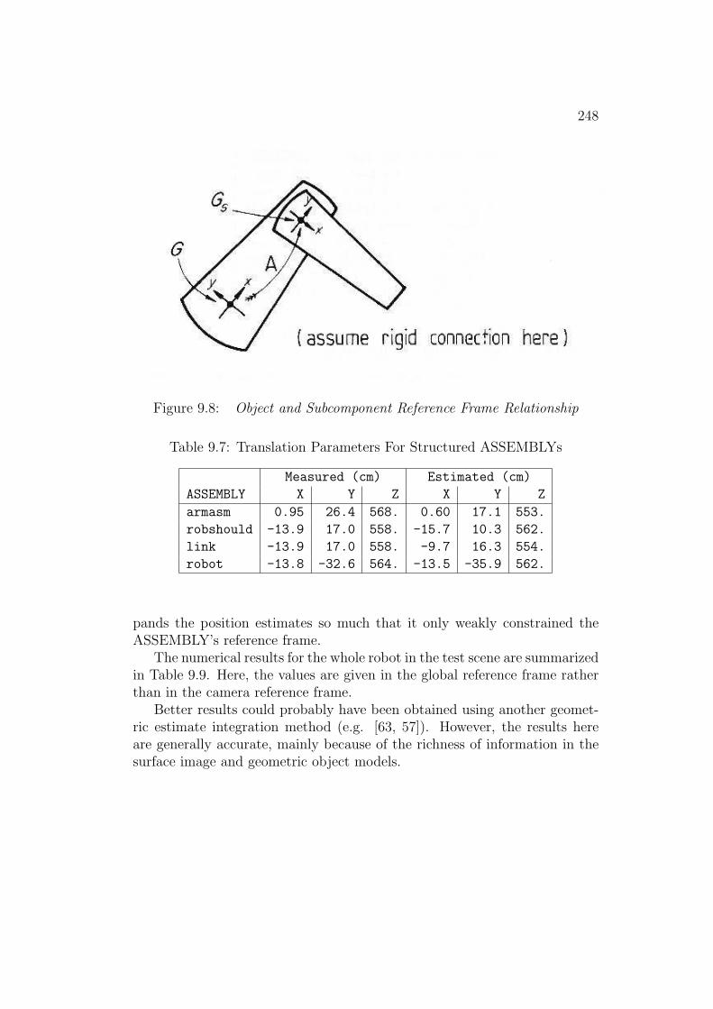
248

Figure 9.8: Object and Subcomponent Reference Frame Relationship

Table 9.7: Translation Parameters For Structured ASSEMBLYs

Measured (cm) Estimated (cm)

ASSEMBLY X Y Z X Y Z

armasm 0.95 26.4 568. 0.60 17.1 553.

robshould -13.9 17.0 558. -15.7 10.3 562.

link -13.9 17.0 558. -9.7 16.3 554.

robot -13.8 -32.6 564. -13.5 -35.9 562.

pands the position estimates so much that it only weakly constrained theASSEMBLY’s reference frame.

The numerical results for the whole robot in the test scene are summarizedin Table 9.9. Here, the values are given in the global reference frame ratherthan in the camera reference frame.

Better results could probably have been obtained using another geomet-ric estimate integration method (e.g. [63, 57]). However, the results hereare generally accurate, mainly because of the richness of information in thesurface image and geometric object models.

249

Table 9.8: Rotation Parameters For Structured ASSEMBLYs

Measured (rad) Estimated (rad)

ASSEMBLY ROT SLANT TILT ROT SLANT TILT

armasm 3.72 2.23 2.66 3.20 2.29 3.11

robshould 0.257 2.23 6.12 0.135 2.29 6.28

link 0.257 2.23 6.12 0.055 2.29 0.05

robot 0.0 0.125 4.73 0.0 0.689 4.75

Table 9.9: Measured And Estimated Spatial Parameters

PARAMETER MEASURED ESTIMATED

X 488 (cm) 486 (cm)

Y 89 (cm) 85 (cm)

Z 554 (cm) 554 (cm)

Rotation 0.0 (rad) 0.07 (rad)

Slant 0.793 (rad) 0.46 (rad)

Tilt 3.14 (rad) 3.53 (rad)

Joint 1 2.24 (rad) 2.18 (rad)

Joint 2 2.82 (rad) 2.79 (rad)

Joint 3 4.94 (rad) 4.56 (rad)

250

9.2.4 Network Based Geometric Reasoning

Position errors result from two causes - errors in the input data and defi-ciencies in the position estimation algorithms. To help remove the secondsource, Fisher and Orr [74] developed a network technique based on the alge-braic method used in ACRONYM. The technique implements the constraintrelationships as a value-passing network that results in tighter bounds andimproved efficiency. Moreover, we observed that the forms of the algebraicconstraints tended to be few and repeated often, and hence standard subnet-work modules could be developed, with instances allocated as new positionconstraints were identified. Examples of these network modules are: “a modelvector is transformed to a data vector” and “a data point must lie near atransformed model point”.

There are three aspects to the new network-based geometric reasoner:

1. specifying the geometric problem as algebraic constraints,

2. evaluating the constraints in a value-passing network and

3. partitioning the network into prototypical modules.

These are now described in more detail.The key data type is the position, which represents the relative spatial

relationship between two features (e.g. world-to-camera, camera-to-model,or model-to-subcomponent). A position consists of a 3-vector representingrelative translation and a unit 4-vector quaternion representing relative ori-entation (of the form (cos(θ/2), sin(θ/2)~w) for a rotation of θ about the axis~w).

The key geometric relationships concern relative position and have twoforms: exact and partially constrained. An example of an exact form is: letobject A be at global position (~rA,~tA), (translation ~tA and rotation ~rA) andobject B be at (~rAB,~tAB) relative to A. Then, the global position of B is:

(rAB ∗ rA, rAB ∗ tA ∗ r′AB + tAB)

where ∗ is the quaternion multiplication operator:

(q0, q1, q2, q3) ∗ (p0, p1, p2, p3)= (q0p0 − q1p1 − q2p2 − q3p3, q2p3 − q3p2 + q0p1 + q1p0,

q3p1 − q1p3 + q0p2 + q2p0, q1p2 − q2p1 + q0p3 + q3p0)

251

and the quaternion inverse operator “ ′ ” is:

(r0, r1, r2, r3)′ = (r0,−r1,−r2,−r3)

A partially constrained position is given by an inequality constraint, suchas:

tAz ≥ 50

This means that the z component of A’s global position is at least 50. Sucha constraint might arise from some a priori scene knowledge, or observing afragment of a surface.

Other relationships concern vectors or points linked by a common trans-formation, as in T~v1 = ~v2, or the proximity of points or vectors:

| ~p1 − ~p2| < ǫ

Instances of these constraints are generated as recognition proceeds. Then,with a set of constraints, it is possible to estimate the values of the con-strained quantities (e.g. object position) from the known model, the datavalues and their relationships. Alternatively, it may be possible to determinethat the set of constraints is inconsistent (i.e. the set of constraints has nosolution), and then the hypothesis is rejected.

A key complication is that each data measurement may have some erroror uncertainty, and hence the estimated values may also have these. Alterna-tively, a variable may be only partially constrained in the model or a prioriscene information. Hence, each numerical quantity is represented by an in-terval [7]. Then, following ACRONYM with some extensions, all constraintsare represented as inequalities, providing either upper or lower bounds on allquantities.

We now look at how the constraints are evaluated.ACRONYM used a symbolic algebra technique to estimate upper (SUP)

and lower (INF) bounds on all quantities. When bounds cross, i.e. SUP (x) <INF (x), then inconsistency was declared and the hypothesis rejected. Thissymbolic algebra method was slow and did not always give tight bounds.

The basis of the network approach is the propagation of updated bounds,through functional units linked according to the algebraic problem specifica-tion. A simple example is based on the inequality:

A ≤ B − C

252

Figure 9.9: Small Constraint Network

By the SUP/INF calculus ([33, 151, 42]), the upper bound of A is constrainedby:

SUP (A) ≤ SUP (B) − INF (C)

as are the lower bounds of B and C:

INF (B) ≥ INF (A) + INF (C)

SUP (C) ≤ SUP (B) − INF (A)

Thus, one can use the value of SUP (B) − INF (C) as an estimated upperbound for A, etc. These relationships are used to create the network forthis single inequality, which is shown in Figure 9.9. As new bounds on (forexample) B are computed, perhaps from other relationships, they propagatethrough the network to help compute new bounds on A and C.

There are two advantages to the network structure. First, because val-ues propagate, local improvements in estimates propagate to help constrainother values elsewhere. Hence, even though we still have rectangular interval

253

parameter space bounds, the constraints are non-rectangular and thus canlink changes in one variable to others. Even for just local problems, contin-ued propagation until convergence produces better results than the symbolicmethods of ACRONYM. Second, these networks have a natural wide-scaleparallel structure (e.g. 1000+) that might eventually lead to extremely fastnetwork evaluation in VLSI (e.g. 10-100 microseconds). One disadvantageof the network approach is that standard bounding relationships must bepre-computed as the network is compiled, whereas the symbolic approachcan be opportunistic when a fortuitous set of constraints is encountered.

For a given problem, the networks can be complicated, particularly sincethere may be both exact and heuristic bounding relationships. For example,the network expressing the reference frame transformation between threepositions contains about 2000 function nodes (of types “+”, “-”, “*”, “/”,“sqrt”, “max”, “greaterthan”, “if” etc.). The evaluation of a network is fast,even in serial, because small changes are truncated to prevent trivial propaga-tions, unlike other constraint propagation approaches (see [53]). Convergenceis guaranteed (or inconsistency detected) because bounds can only tighten(or cross), since only sufficiently large changes are propagated.

The creation of the networks is time-consuming, requiring a symbolicanalysis of the algebraic inequalities. Fortunately, there is a natural modularstructure arising from the types of problems encountered during scene anal-ysis, where most geometric constraints are of a few common types. Hence, itis possible to pre-compile network modules for each relationship, and merelyallocate a new instance of the module into the network as scene analysisproceeds. To date, we have identified and implemented network modules for:

SS - two scalars are close in value

PP - two points are close in location

VV - two vectors point in nearly the same direction

TP - a transformation links a pair of points

TV - a transformation links a pair of vectors

TV2 - a transformation links two pairs of vectors

TT - a transformation links from one position to a second by a third position

P2V - a vector can be defined by two points

254

QWT - a quaternion is equivalent to an axis of rotation and an angle

One important feature of these modules is that they are bi-directional,in that each variable partially constrains all other related variables. Hence,this method is usable for expressing partial constraints (such as “the objectis above the table” or Z ≥ 0). The constraints on other related variables canthen help fully constrain unbound or partially constrained variables.

We now include a simple and a complicated example of network use.Suppose subcomponents B and C are rigidly connected to form object A.With the estimated positions of the subcomponents in the global coordinatesystem, Pg−B and Pg−C , and the transformations between the object andlocal coordinate systems, PA−B and PA−C , then these can be used to estimatethe global object position, Pg−A, by using two instances of the “TT” modulelisted above. Figure 9.10 shows this network. Notice that each subcomponentgives an independent estimate of Pg−A, so that the network keeps the tightestbounds on each component of the position. Any tighter resulting bounds thenpropagate back through the modules to refine the subcomponent positionestimates.

Figure 9.11 shows the full network generated for analyzing the robot inthe test scene. As before, the boxes represent transformations, but thereare more types used here. The “TPn” boxes stand for n instances of a“TP” module. The circular “Jn” boxes represent three identical instances ofsubnetworks allocated for transformations involving joint angles, which areomitted to simplify the diagram (each contains 7 network modules). Therelative positions of objects are given by the P structures, such as Pg−R,which represents the position of the robot in the global reference frame.These are linked by the various transformations. Links to model or datavectors or points are represented by the unconnected segments exiting fromsome boxes.

The top position Pg−C is the position of the camera in the global coordi-nate system, and the subnetwork to the left and below relates features in thecamera frame to corresponding ones in the global coordinate system. Belowthat is the position Pg−R of the robot in the global coordinate system andthe position PC−R of the robot in the camera coordinate system, all linked bya TT position transformation module. Next, to the bottom left is the sub-network for the cylindrical robot body Pg−B. The “J1” node connects therobot position to the rest (“link”) on the right, whose position is Pg−LK . Itsleft subcomponent is the rigid shoulder ASSEMBLY (SH) with its subcom-

255

Rigid Subcomponent Hierarchy

A

��

��

��

��

��

AAAAAAAAAA

PA−B PA−C

B C

Corresponding Geometric Network

Pg−A

��

��

AAAA

TT TTPA−B PA−C

Pg−B Pg−C

Figure 9.10: A Simple Geometric Reasoning Network

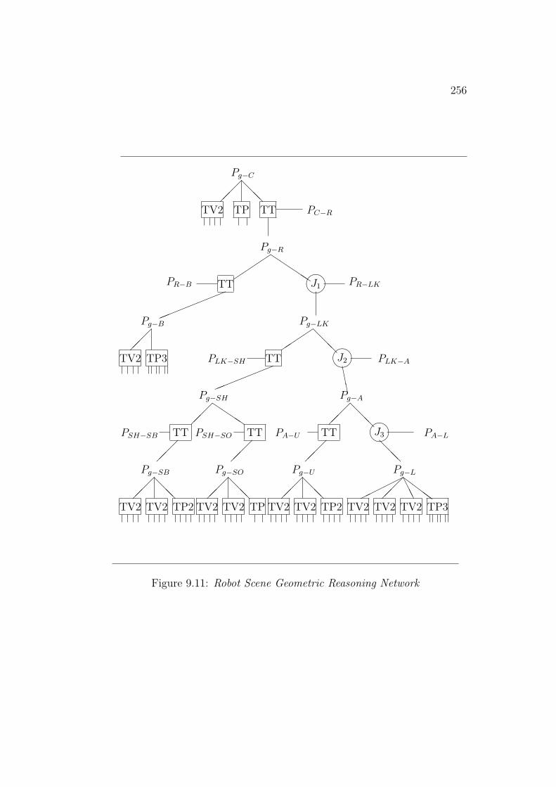
256

Pg−C

���

@@@

TV2 TP TT PC−R

Pg−R

��

��

QQ

QQQPR−B TT J1��

��PR−LK

!!!!!!!!Pg−B Pg−LK

���

@@@

��

��TV2 TP3 PLK−SH TT J2��

��PLK−A

DDD

!!!!!!!Pg−SH Pg−A

���

QQ

QQ�

��@

@@PSH−SB TT PSH−SO TT PA−U TT J3��

��PA−L

���

���

���

@@@

Pg−SB Pg−SO Pg−U Pg−L

���

@@@

���

@@@

���

@@@

������

��AAA

ZZ

ZZTV2 TV2 TP2 TV2 TV2 TP TV2 TV2 TP2 TV2 TV2 TV2 TP3

Figure 9.11: Robot Scene Geometric Reasoning Network

257

ponents, the shoulder body (SB) and the small shoulder patch (SO). To theright, the “J2” node connects to the “armasm” ASSEMBLY (A), linking theupper arm (U) to the lower arm (L), again via another joint angle (“J3”). Atthe bottom are the modules that link model vectors and points to observedsurface normals, cylindrical axis vectors, and central points, etc. Altogether,there are 61 network modules containing about 96,000 function nodes.

The network structure closely resembles the model subcomponent hier-archy, and only the bottom level is data-dependent. There, new nodes areadded whenever new model-to-data pairings are made, producing new con-straints on feature positions.

Evaluating the complete network from the raw data requires about 1,000,000node evaluations in 800 “clock-periods” (thus implying over 1000-way par-allelism). Given the simplicity of operations in a node evaluation, a futuremachine should be able to support easily a 1 microsecond cycle time. Thissuggests that an approximate answer to this complicated problem could beachieved in about 1 millisecond.

As the tolerances on the data errors propagate through the network mod-ules, they do not always produce tight result intervals, though some intervalreduction is achieved by integrating separate estimates. For example, if eachorientation component of a random position Pa−b has interval width (i.e. er-ror) δ and each orientation component of a random position Pb−c has intervalwidth ǫ, then each component of the resulting position Pa−c = Pa−b ∗ Pb−c

has interval width:16(δ + ǫ)

3π

However, this interval width is less or non-existent for most of the actualrigid transformations used here.

Because the resulting intervals are not tight, confidence that the meaninterval value is the best estimate is reduced, though the bounds are correctand the mean interval values provide useful position estimates. To tightenestimates, a post-processing phase iteratively shrinks the bounds on a se-lected interval and lets the new bounds propagate through the network. Forthe robot example, this required an additional 12,000 cycles, implying a totalsolution time of about 13 milliseconds on our hypothetical parallel machine.

Using the new geometric reasoning network, the numerical results for thewhole robot in the test scene are summarized in Table 9.10. Here, the valuesare given in the global reference frame rather than in the camera referenceframe.

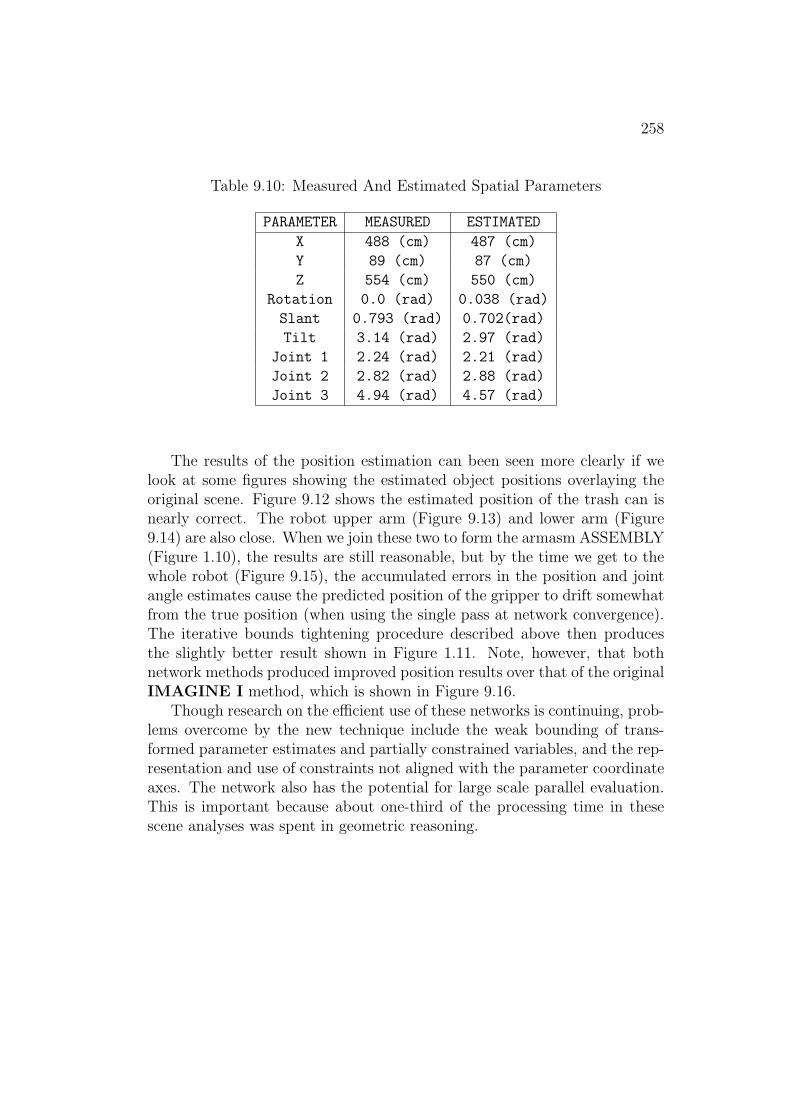
258

Table 9.10: Measured And Estimated Spatial Parameters

PARAMETER MEASURED ESTIMATED

X 488 (cm) 487 (cm)

Y 89 (cm) 87 (cm)

Z 554 (cm) 550 (cm)

Rotation 0.0 (rad) 0.038 (rad)

Slant 0.793 (rad) 0.702(rad)

Tilt 3.14 (rad) 2.97 (rad)

Joint 1 2.24 (rad) 2.21 (rad)

Joint 2 2.82 (rad) 2.88 (rad)

Joint 3 4.94 (rad) 4.57 (rad)

The results of the position estimation can been seen more clearly if welook at some figures showing the estimated object positions overlaying theoriginal scene. Figure 9.12 shows the estimated position of the trash can isnearly correct. The robot upper arm (Figure 9.13) and lower arm (Figure9.14) are also close. When we join these two to form the armasm ASSEMBLY(Figure 1.10), the results are still reasonable, but by the time we get to thewhole robot (Figure 9.15), the accumulated errors in the position and jointangle estimates cause the predicted position of the gripper to drift somewhatfrom the true position (when using the single pass at network convergence).The iterative bounds tightening procedure described above then producesthe slightly better result shown in Figure 1.11. Note, however, that bothnetwork methods produced improved position results over that of the originalIMAGINE I method, which is shown in Figure 9.16.

Though research on the efficient use of these networks is continuing, prob-lems overcome by the new technique include the weak bounding of trans-formed parameter estimates and partially constrained variables, and the rep-resentation and use of constraints not aligned with the parameter coordinateaxes. The network also has the potential for large scale parallel evaluation.This is important because about one-third of the processing time in thesescene analyses was spent in geometric reasoning.

259

Figure 9.12: Recognized Trash Can

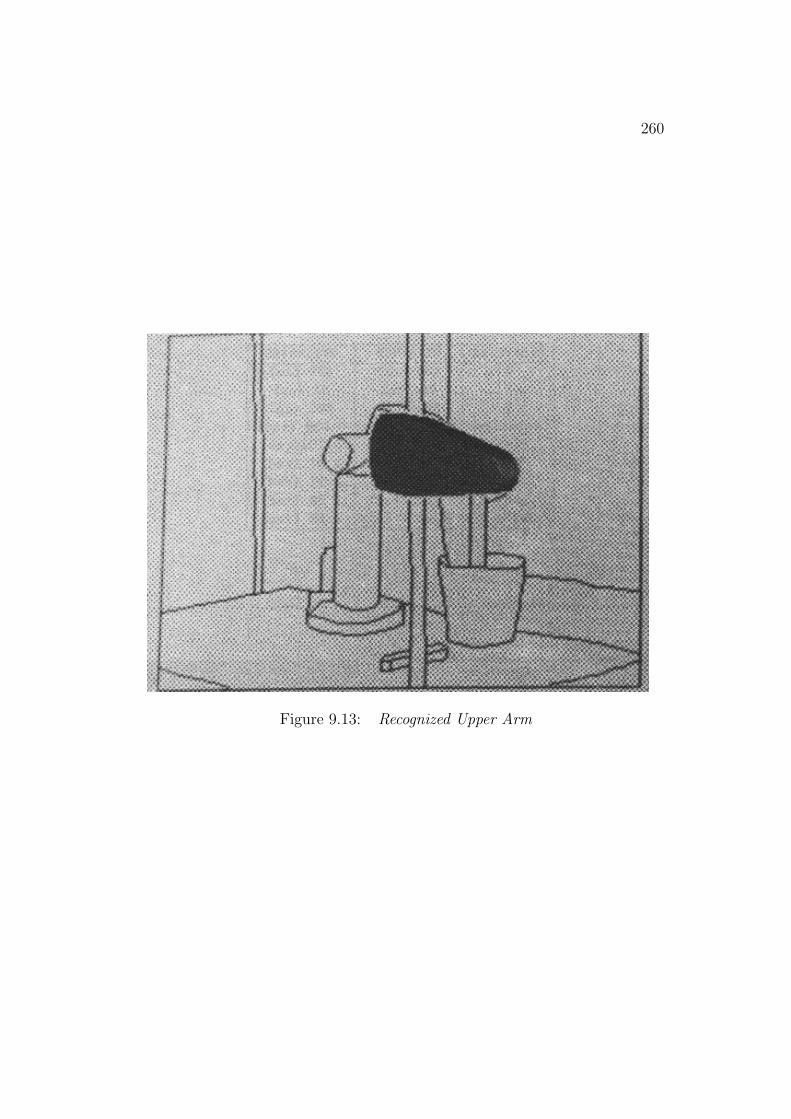
260

Figure 9.13: Recognized Upper Arm

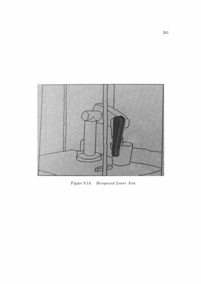
261

Figure 9.14: Recognized Lower Arm

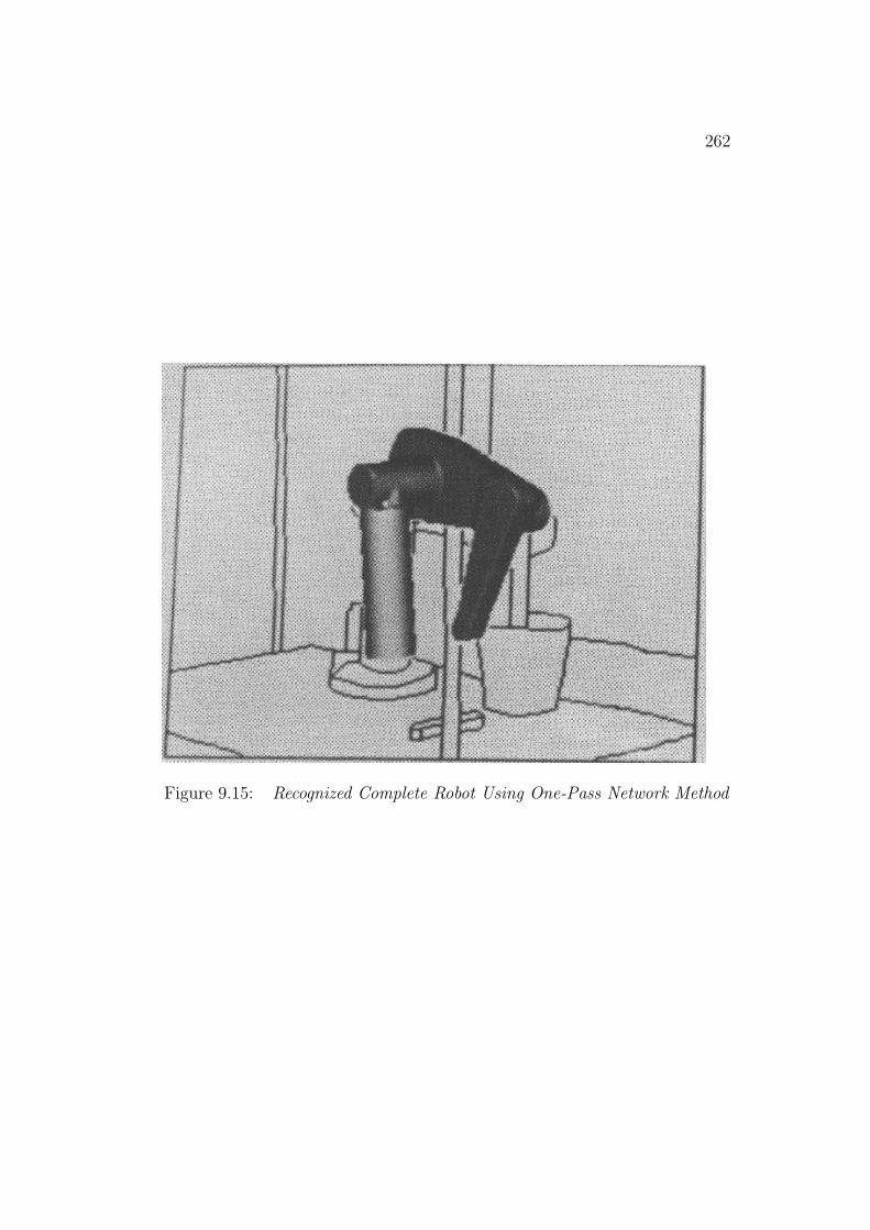
262

Figure 9.15: Recognized Complete Robot Using One-Pass Network Method

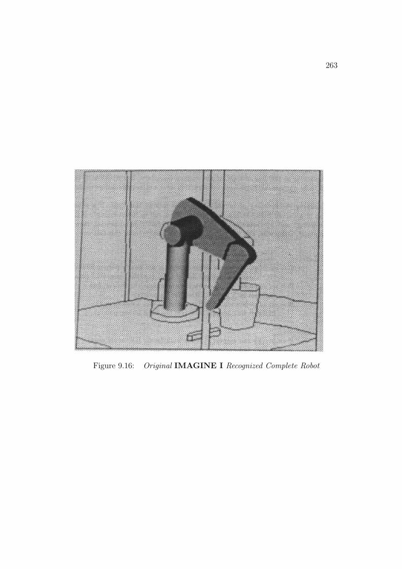
263

Figure 9.16: Original IMAGINE I Recognized Complete Robot

264

9.3 Feature Visibility Analysis

In three dimensional scenes, not all object features will be visible (e.g. somewill be on the back side of an object), and a true three dimensional sceneunderstanding program should account for this. There are three distinctcases of feature invisibility. The first case always occurs: there are featureson the back side of every object and these cannot ordinarily be detected froma single viewpoint (except by using mirrors or shadows). At the same time,it is easy to predict what cannot be seen, using the estimated orientation ofhypotheses to predict back-facing SURFACEs.

The next case is forward-facing self-obscured features. Here, an objectfeature is obscured by one or more closer surfaces from the same object.Given knowledge of the object’s shape and position relative to the viewer,the relative surface positions and their visibility can be predicted.

Finally, there is structure obscured by unrelated objects. Here, the detailsof occlusion cannot be predicted, nor is it easy to deduce the invisible struc-ture (though context and historical information could help – as in the top ofa desk). Perhaps the best that can be done is to show that what remains isconsistent with the hypothesis of obscured structure. Consequently, indirectevidence for some features must be found. This requires three actions – pre-dicting feature visibility, finding evidence for closer structures and verifyingthat the available features up to the point of occlusion are consistent withthe model.

After feature visibility analysis, the results are used in three ways:

1. SURFACEs predicted to be invisible are not searched for,

2. SURFACEs predicted to be partially self-obscured are verified as hav-ing one or more boundaries that show this (e.g. back-side obscuringbetween this and other object SURFACEs), and

3. SURFACEs predicted to be completely visible are verified as having noback-side obscuring boundaries (unless obscured by unrelated objects).

Because of parameter estimation errors, test 3 is not reliable and is notperformed (more discussion below).

These three cases of feature visibility are only applied to individual SUR-FACEs, as any ASSEMBLY can be decomposed into SURFACEs.

265

9.3.1 Deducing Back-Facing SURFACEs

Deducing whether planar SURFACEs are back-facing or not is simple: if thepredicted surface normal points away from the camera, then the SURFACEis not visible.

Let:~n be the model SURFACE normal ((0, 0, -1) by definition)A be the coordinate transformation from the SURFACE’s

local system to that of the whole objectG be the transformation from the object’s

local system to that of the camera~p = a nominal point on the SURFACE in local coordinates

Then:~m = GA~n is the predicted normal orientation~v = GA~p is the view vector from the camera to the point

on the SURFACETest:

if ~v ◦ ~m > 0, then the SURFACE is back-facing

For curved SURFACEs, we test the normal at each point on the boundary.By the segmentation assumptions (Chapter 3), the surface varies smoothlywithin the boundaries, so if all points on the boundary and the nominalcentral point are back-facing, then the interior of the surface almost alwaysis as well.

A problem occurs with the combination of nearly tangential SURFACEsand parameter misestimation. Here, SURFACEs predicted as visible maynot always be so, and vice versa. This case can be detected, by detectingsurface normals oriented nearly perpendicular to the line of sight at thesurface boundary. If a SURFACE is determined to be tangential, hypothesisconstruction does not require image evidence for it.

Classifying the visibility of curved SURFACEs follows this logic: If asubstantial portion of a curved SURFACE is front-facing, then call it “front-facing”. If it is not “front-facing” and a substantial portion of the SURFACEis tangential, then call it “tangential”. Otherwise, call it “back-facing”. Theideal form of this test is:

266

Let:T = set of points whose surface normals are nearly perpendicular to

the three dimensional line of sight (i.e. the tangential points)F = set of points whose surface normals face the viewer, but

are not in T (i.e. the front-facing points)B = set of points whose surface normals face away from the

viewer, but are not in T (i.e. the back-facing points)Then:

If empty(F) and empty(T), then back-facing (i.e. never seen)If empty(F) and not(empty(T)), then tangential (i.e. possibly seen)If not(empty(F)), then front-facing (i.e. always seen)

Because of parameter estimation errors, some compromises in the aboveideal algorithm are made:

• thresholds are added to decide the visibility class of each vector

• thresholds are added to decide the visibility class of the whole SUR-FACE

The algorithm to classify individual vectors is:

Let:~vi be the line of sight to point i~mi be the predicted surface normal vector at idi = ~vi ◦ ~mi

Then:if di > τ1, then i ∈ B (τ1 = 0.1)if di < −τ1, then i ∈ Fi ∈ T otherwise

267

Table 9.11: Predicted SURFACE Visibility

Object SURFACE Visibility

robbody front-facing = {robbodyside(1)}tangential = {robbodyside(2)} *1

robshldbd front-facing = {robshldend,robshould2}tangential = {robshould1} *1

robshldsobj front-facing = {robshoulds(1)}tangential = {robshoulds(2)} *1

upperarm front-facing = {uside(2),uends,uedgel(1)}back-facing = {uside(1),uendb,uedgel(2)}tangential = {uedges(1),uedges(2)}

lowerarm front-facing = {lsideb,ledgea,lendb}back-facing = {lsidea,ledgeb}

trashcan front-facing = {tcanoutf(1),tcaninf(1),tcanbot(1)}

back-facing = {tcanbot(2)}tangential = {tcanoutf(2),tcaninf(2)} *1

*1 – largely back-facing curved SURFACE has tangential sides

The classification of the whole SURFACE is obtained by:Let:

b = size(B)f = size(F)t = size(T)s = b + f + t

Then:if f/s > τ2, then front-facing (τ2 = 0.1)else if t/s > τ3, then tangential (τ3 = 0.1)else back-facing

When this classification was applied to the objects with their estimatedreference frames in the test image, surface visibility was correctly deduced.The results are shown in Table 9.11.

268

9.3.2 Deducing Self-Obscured SURFACEs

Given the deductions of the previous subsection, all remaining SURFACEsmust be at least partially front-facing, but some may be partially or whollyself-obscured by other closer SURFACEs from the same object.

Self-occlusion analysis uses the object model and position estimates topredict an image of the object, which is then analyzed for visibility. Theprocess occurs in three stages:

1. prediction of visible SURFACEs,

2. deduction of missing SURFACEs and

3. deduction of partially self-obscured SURFACEs.

The first step is implemented using a raycasting depth image generator.Here, a ray from the viewer is intersected with the model SURFACEs placedaccording to the object’s estimated position. The raycaster produces anarray of pixels valued with the depth and identity of the closest (i.e. visible)SURFACE.

The detection of completely obscured structure is now trivial and consistsof finding those front-facing SURFACEs (from the analysis of the precedingsubsection) not visible in the predicted image.

The detection of partially obscured SURFACEs is also simple. Duringimage generation, whenever a predicted visible surface pixel was replaced ornot included because of a closer pixel, then self-occlusion occurred. The iden-tities of all SURFACEs that suffered this are recorded during the generationof the synthetic image. Any such SURFACE not completely self-obscured isthen partially self-obscured.

Parameter estimation errors may cause nearly obscured SURFACEs todisappear and barely obscured SURFACEs to reappear. A similar effect oc-curs with unobscured SURFACEs becoming partially obscured (i.e. becausea closer SURFACE moves slightly in front of it) and vice versa. So, thefollowing algorithm was implemented to decide the visibility classes:

269

Figure 9.17: Boundaries Surround Completely Obscured Surface

Let:v = number of visible pixels (predicted by raycasting)n = number of obscured pixels (predicted by raycasting)p = v/(v + n) (percentage of visible pixels)

Then:if p > τ1, then the SURFACE is fully visible (τ1 = 0.9)if τ1 ≥ p > τ2, then the SURFACE is partially obscured (τ2 = 0.05)Otherwise, the SURFACE is fully obscured

Table 9.12 records the predicted occlusion status for all front-facing SUR-FACEs of all primitive ASSEMBLYs in the test image. This correspondsexactly to the observed visibility of all SURFACEs (disregarding externalocclusion, which is discussed below). For structured ASSEMBLYs, the pro-cess is similar, only some previous cases of external occlusion now becomeself-occlusion as components are connected together.

9.3.3 Detecting External Occlusion

Structure obscured by unrelated objects cannot be anticipated in coinciden-tal scene arrangements, unless closer objects can be identified. What remains

270

Table 9.12: Predicted Self-Occlusions

Object Occlusion Status

robbody fully-visible = {robbodyside(1)}robshldbd fully-visible = {robshldend,robshould2}robshldsobj fully-visible = {robshoulds(1)}upperarm fully-visible = {uside(2),uends}lowerarm fully-visible = {lsideb,ledgea}

partially-self-obscured = {lendb}trashcan fully-visible = {tcanoutf(1)}

partially-self-obscured = {tcaninf(1)}fully-self-obscured = {tcanbot(1)}

possible is to show that the absence of a feature is consistent with the as-sumption of occlusion, that is, there are closer, unrelated surfaces completelycovering the portion of the image where it is expected. This unrelatednesscan be verified by detecting front-surface-obscuring or concave boundariescompletely surrounding the closer surfaces, as in Figure 9.17.

The other case considered occurs when non-self-obscured SURFACEs areobserved as partially obscured. These must meet all shape and adjacencyconstraints required by the model and the invisible portions must be to-tally behind other unrelated surfaces (as before). The boundary between thepartial object and obscuring surfaces must be obscuring.

Verifying fully obscured structure is the simplest case. Here, every portionof the predicted model SURFACE must be behind an unrelated data surface.Minor errors in absolute distance prediction make it difficult to directly verifythat an object surface pixel is further away than the corresponding observedpixel, such as when a piece of paper lies on a table surface. Fortunately,relative surface depth differences have already been accounted for in thelabeling of obscuring boundaries and the formation of depth ordered surfaceclusters (Chapter 5). The ordering test can then be reformulated to verifythat the entire missing SURFACE lies within the image region belonging toan unrelated, closer, surface cluster. In practice, the test can be performedusing a raycasting technique:

1. Find the set of closer, unrelated surfaces.

271

2. Predict the image locations for the missing SURFACE.

3. For each pixel, verify that the observed surface image region has beenassigned to one of the closer surfaces.

Again, this ideal algorithm was altered to tolerate parameter misestima-tion:

Let:P = set of predicted image positions for the SURFACEI = subset of P lying on identified object surfaces

(should be empty)O = subset of P lying on closer unrelated obscuring

surfaces (should be P)E = subset of P lying elsewhere (should be empty)

If:size(I) / size(P) < τ1 and size(E) / size(O) < τ2

(τ1 = 0.2, τ2 = 0.2)

Then: declare the surface to be externally obscured

Figure 9.18 illustrates the test.Because of the depth ordering ambiguities of concave surface boundaries

(i.e. which surface, if either, is in front of the other), this approach willfail to detect some cases of external occlusion. Difficulties also occur withsurfaces that lie both in front of and behind objects. In the absence ofmore accurate depth predictions, the only correct test may be to observean obscuring boundary between the visible portions of the object and themissing portions.

The only fully externally obscured structure was the robot hand, whichwas correctly detected. Because the reference frame estimates for the lower-arm had a slightly larger rotation angle, part of the hand was predicted notto be obscured by the trash can. This motivated the threshold based testdescribed above.

Figure 9.19 shows the predicted position of the robot hand on top of thescene.

Determining the visibility status of the model features was computa-tionally expensive – particularly the raycasting image generation for self-occlusion analysis. About one-third of the processing time was spent in this

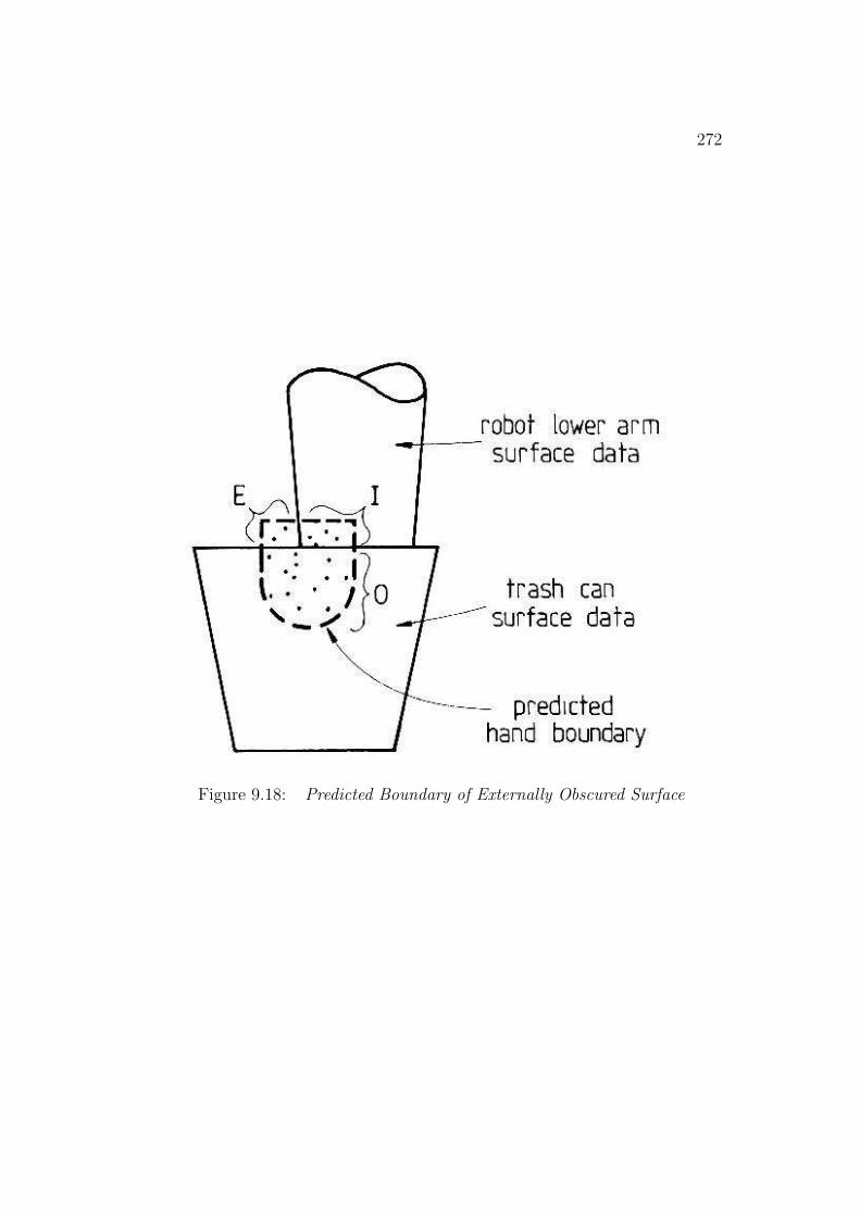
272

Figure 9.18: Predicted Boundary of Externally Obscured Surface

273

Figure 9.19: Predicted Gripper Position

274

process. In response to this, the SMS modeling approach [70] was developed.These models explicitly record the visibility of all model features for the SMSequivalent of each ASSEMBLY, for the key viewpoints. The model does notspecify the visibility relationship of all recursively accessible features, merelythose represented at the current level of the hierarchy, which considerablyreduces the number of occlusion relationships considered for each object.Feature visibility is associated with a partitioning of the view sphere, andthe relative position between the viewer and the object determines whichpartition applies at a given time. From this index, the visibility is directlyaccessed.

9.4 Direct Evidence Collection

The visibility analysis deduced the set of SURFACEs for which image evi-dence should be available and we now discuss how such evidence is detectedand matched to the model.

9.4.1 Initial (Invocation) Feature Evidence

Model SURFACEs have no substructure, so the evidence for a hypothesizedmodel SURFACE is the associated surface image region. ASSEMBLYs arethen formed by hierarchical synthesis [161], so previously verified subcompo-nents or SURFACE hypotheses are evidence for a hypothesized ASSEMBLY.

If invocation occurs, at least one subcomponent grouping (Section 8.2.3)must have positive plausibility, which suggests that some subcomponentsare visible and are likely to have been previously recognized. (If none wereinvoked, then it is unlikely that the object will be invoked.) Then, verifiedsubcomponent hypotheses become the initial evidence for the structure.

For each image structure associated with the invocation subcomponentgroup, all verified hypotheses of the correct types in the current image context(surface cluster) are located. Then, groups of these verified subcomponenthypotheses are combinatorially paired with the invoked model’s features tocreate a new hypothesis, provided that:

1. Each model feature gets at most one hypothesis, which must have thecorrect type.

2. No image structure is used more than once.

275

3. Only maximal pairings are considered.

4. There is a consistent reference frame that unifies all subcomponents.

The combinatorial matching is potentially explosive, but each image sub-structure generally has only a few verified hypotheses, usually arising fromsymmetry or ambiguity. Objects with these problems or duplicated featuresgenerate more initially consistent hypotheses, but most of these are elimi-nated by constraints (2) and (4).

The worst combinatorial explosion occurs with the robot lower arm, whereeach of the visible planar surfaces could be one of two model SURFACEs, eachin two possible orientations. The curved end SURFACE has one model in twopossible orientations. Altogether, there are initially 32 possible pairings usingpreviously recognized subcomponents. Fortunately, the constraints eliminateall but two, which are indistinguishable in this scene. The upper arm is thenext worst case, with eight initial pairings of which two are left after theconstraints. All other initial hypothesis generations had four or fewer cases.Most invalid cases were eliminated by constraint (4).

9.4.2 Additional SURFACE Feature Location

Given the initial location estimates and the geometric model, it is easy topredict where a visible surface should appear. This prediction simplifiesdirect search for image evidence for the feature. This is, in style, like thework of Freuder [75], except that three dimensional scenes are consideredhere.

To select good image evidence for an uninstantiated model feature, theoriented model is used to predict roughly where the surface data shouldappear. Figure 9.20 shows the predicted location for the robot upper armuedgel panel superimposed on the original image using the initial parameterestimates for upperarm.

Other constraints can then be applied to eliminate most inappropriatesurfaces from the predicted area. The constraints that a potential surfacemust meet are:

1. It must not be previously used.

2. It must be in the surface cluster for the ASSEMBLY.

3. It must be in the correct image location.

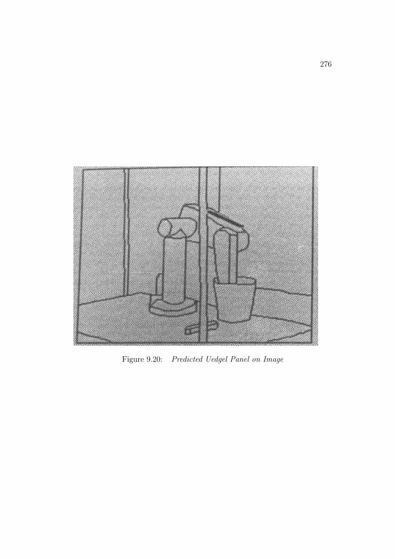
276

Figure 9.20: Predicted Uedgel Panel on Image

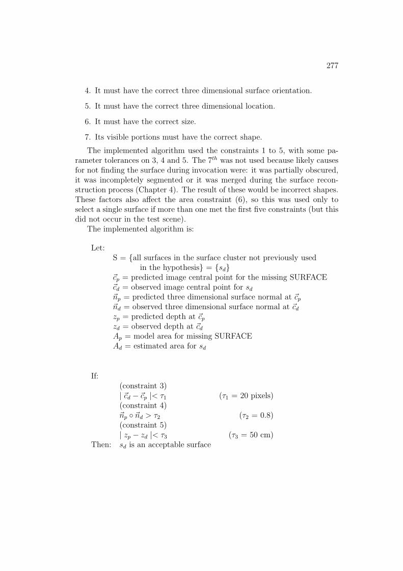
277

4. It must have the correct three dimensional surface orientation.

5. It must have the correct three dimensional location.

6. It must have the correct size.

7. Its visible portions must have the correct shape.

The implemented algorithm used the constraints 1 to 5, with some pa-rameter tolerances on 3, 4 and 5. The 7th was not used because likely causesfor not finding the surface during invocation were: it was partially obscured,it was incompletely segmented or it was merged during the surface recon-struction process (Chapter 4). The result of these would be incorrect shapes.These factors also affect the area constraint (6), so this was used only toselect a single surface if more than one met the first five constraints (but thisdid not occur in the test scene).

The implemented algorithm is:

Let:S = {all surfaces in the surface cluster not previously used

in the hypothesis} = {sd}~cp = predicted image central point for the missing SURFACE~cd = observed image central point for sd

~np = predicted three dimensional surface normal at ~cp

~nd = observed three dimensional surface normal at ~cd

zp = predicted depth at ~cp

zd = observed depth at ~cd

Ap = model area for missing SURFACEAd = estimated area for sd

If:(constraint 3)| ~cd − ~cp |< τ1 (τ1 = 20 pixels)(constraint 4)~np ◦ ~nd > τ2 (τ2 = 0.8)(constraint 5)| zp − zd |< τ3 (τ3 = 50 cm)

Then: sd is an acceptable surface

278

The surface selected is the acceptable sd whose area is closest to thatpredicted, by minimizing:

| 1 − Ad

Ap

|

In the test image, the only missing SURFACEs were the two side surfaceson the upper arm and the inside surface at the back of the trash can. For thetrash can, the only potential image surfaces for the trash can back surfacewere the two visible surfaces in the surface cluster. The front surface wasalready used in both cases, and the rear surface met all the other constraints,so was selected. A similar process applied to the upper arm side panels.

9.4.3 Rigid Subcomponent Aggregation

Surfaces are not the only evidence accepted for model features – previouslyrecognized subcomponents are also used. For example, a nose would be sucha subcomponent in the context of a face. The structures can be rigidlyconnected to the parent object (e.g. nose to face) or non-rigidly connected(e.g. arm to body). The collections should correspond to model featuresbecause of the model segmentation assumptions (Chapter 7) and the surfacecluster formation process (Chapter 5).

Any analysis associated with these structures can be reduced to analysisof the subcomponent SURFACEs, but it would be desirable to use the largerunits. First, the substructures might have been previously identified, and soprocessing should not be duplicated, and second, the use of larger structuralunits helps reduce the combinatorial matching. Finally, parsimony dictatesthat matching should proceed at the level of descriptions, and complex ob-jects would be described using subcomponents.

Because of the hierarchical synthesis [161] nature of the recognition pro-cess, previously recognized subcomponents can be directly integrated as evi-dence, without having to return to the surface analysis [66]. As the subcom-ponent’s type is already a strong constraint on its usability, the remainingconstraints are:

1. being in the surface cluster,

2. having the correct adjacent structure and

3. having correct placement.

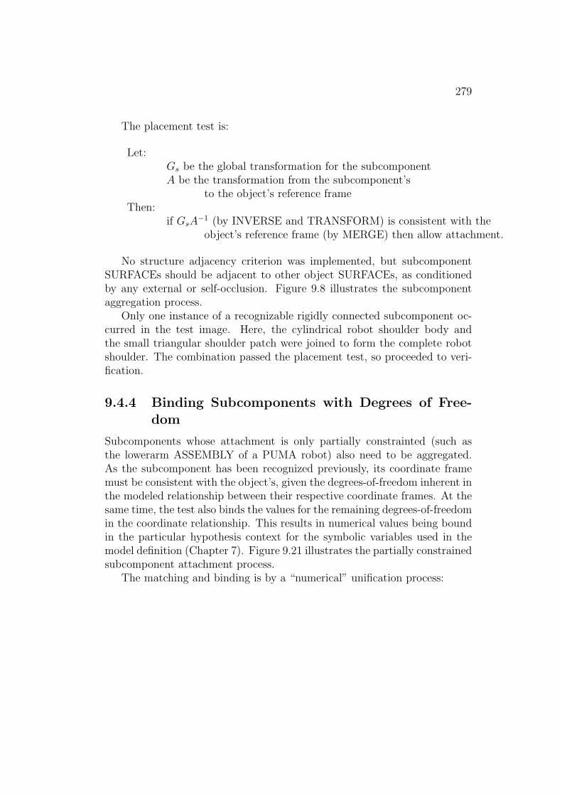
279

The placement test is:

Let:Gs be the global transformation for the subcomponentA be the transformation from the subcomponent’s

to the object’s reference frameThen:

if GsA−1 (by INVERSE and TRANSFORM) is consistent with theobject’s reference frame (by MERGE) then allow attachment.

No structure adjacency criterion was implemented, but subcomponentSURFACEs should be adjacent to other object SURFACEs, as conditionedby any external or self-occlusion. Figure 9.8 illustrates the subcomponentaggregation process.

Only one instance of a recognizable rigidly connected subcomponent oc-curred in the test image. Here, the cylindrical robot shoulder body andthe small triangular shoulder patch were joined to form the complete robotshoulder. The combination passed the placement test, so proceeded to veri-fication.

9.4.4 Binding Subcomponents with Degrees of Free-dom

Subcomponents whose attachment is only partially constrainted (such asthe lowerarm ASSEMBLY of a PUMA robot) also need to be aggregated.As the subcomponent has been recognized previously, its coordinate framemust be consistent with the object’s, given the degrees-of-freedom inherent inthe modeled relationship between their respective coordinate frames. At thesame time, the test also binds the values for the remaining degrees-of-freedomin the coordinate relationship. This results in numerical values being boundin the particular hypothesis context for the symbolic variables used in themodel definition (Chapter 7). Figure 9.21 illustrates the partially constrainedsubcomponent attachment process.

The matching and binding is by a “numerical” unification process:

280

Figure 9.21: Partially Constrained Subcomponent Aggregation (in 2D)

Let:G be the global reference frame transformation for the objectS be the global reference frame transformation for the subcomponentA(~x) be the transformation from the subcomponent’s reference frame

to the object’s reference frame with ~x as the unbound variablesThen:

Compare G−1S to A(~x)Where A(~x) has bound variables, then the values must match

(i.e. parameter estimate ranges overlap)Where A(~x) has unbound variables, then the variables are set

to the corresponding parameter ranges from G−1S

The results for the correct partially constrained subcomponent aggrega-tions are summarized in Table 9.13. All correct bindings were made, and thetable shows that the connection parameters were estimated well. Most of theincorrect combinatorial subcomponent groupings were eliminated during thebinding process because of inconsistent reference frames, so this was also abenefit.

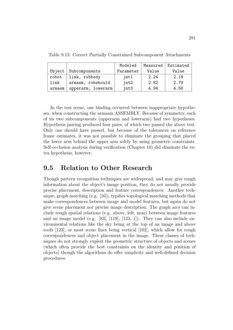
281

Table 9.13: Correct Partially Constrained Subcomponent Attachments

Modeled Measured Estimated

Object Subcomponents Parameter Value Value

robot link, robbody jnt1 2.24 2.18

link armasm, robshould jnt2 2.82 2.79

armasm upperarm, lowerarm jnt3 4.94 4.56

In the test scene, one binding occurred between inappropriate hypothe-ses, when constructing the armasm ASSEMBLY. Because of symmetry, eachof its two subcomponents (upperarm and lowerarm) had two hypotheses.Hypothesis pairing produced four pairs, of which two passed the above test.Only one should have passed, but because of the tolerances on referenceframe estimates, it was not possible to eliminate the grouping that placedthe lower arm behind the upper arm solely by using geometric constraints.Self-occlusion analysis during verification (Chapter 10) did eliminate the ex-tra hypothesis, however.

9.5 Relation to Other Research

Though pattern recognition techniques are widespread, and may give roughinformation about the object’s image position, they do not usually provideprecise placement, description and feature correspondences. Another tech-nique, graph matching (e.g. [16]), typifies topological matching methods thatmake correspondences between image and model features, but again do notgive scene placement nor precise image description. The graph arcs can in-clude rough spatial relations (e.g. above, left, near) between image featuresand an image model (e.g. [83], [119], [123, 1]). They can also include en-vironmental relations like the sky being at the top of an image and aboveroofs [123], or most scene lines being vertical [102], which allow for roughcorrespondences and object placement in the image. These classes of tech-niques do not strongly exploit the geometric structure of objects and scenes(which often provide the best constraints on the identity and position ofobjects) though the algorithms do offer simplicity and well-defined decisionprocedures.

282

Geometric scene understanding systems can be classified by the dimen-sionality of their model features (i.e. point, curve, region or volume) andtheir image data (i.e. two or three dimensional). All of the key researchdiscussed below used three dimensional geometric models.

Early scene understanding systems (e.g. [139, 60]) used two dimensionalpoint or corner correspondences to solve for object location and projectionrelationships. Later, Turner [161] located objects by using three dimen-sional points found from stereo triangulation of paired two dimensional imagepoints.

Three influential edge-based recognition systems are:

• Brooks’ ACRONYM system [42] matched pairs of nearly parallel twodimensional lines (“ribbons”) to the extremal boundaries of general-ized cylinders, thus instantiating model primitives. Larger objects werefound by a graph matching technique, where the arcs in the graphs rep-resented two dimensional projections of three dimensional geometricrelationships between the generalized cylinders (e.g. relative orienta-tion). Three dimensional object position was found by using the twodimensional image measurements (feature sizes and positions, etc.) toback-constrain the range of position parameters.

• Lowe’s SCERPO system [108] used groupings of straight two dimen-sional line features to suggest and orient model instances - which weresets of three dimensional lines. To help avoid combinatorial matchingproblems, he used a “perceptual organization” technique that groupededges by colinearity, parallelism and endpoint connectivity and thenformed larger features, like parallelograms. A measure of significancerelated to the probability of random occurrence of the segment group-ings was calculated for both model and data segments, which was thenused to help order search. With a pairing of three or more segments,three dimensional position was found by using an iterative least-squarederror algorithm. Hypotheses were then verified and refined by collect-ing additional line evidence, using direct feature predictions from theinitial position estimates.

• The University of Sheffield TINA system [134] matched three dimen-sional lines derived from binocular stereo to a three dimensional wireframe object model (which was itself derived empirically from observed

283

instances of the objects). The use of edge information implied the ob-jects needed to be largely polyhedral. A least-squared error matchingprocess deduced the position of the object from the three dimensionalfeature correspondences.

Lowe’s work was analyzed by McIvor [114], with the main criticisms beingover weak initial position estimates, ignoring edge fragmentation, incorrectprobability analysis for larger groups, unnecessary projection relationshipsimplifications and insufficient discriminatory powers. However, McIvor alsodemonstrated the approach was successful in 10 of 16 views of a test part.

There has been little geometric matching of two dimensional image re-gions to three dimensional model surfaces. Fisher [66] used heuristics basedon the deformations of the three dimensional model surface patches whenseen in two dimensions to estimate three dimensional surface patch position.This supported a hierarchical synthesis matching process that recognizedlarger objects. Ballard and Sabbah [13] used a variety of Hough transfor-mation techniques to estimate the six positional parameters sequentially.This uniform mechanism is more stable to noise, but is likely to suffer whenthe object’s shape varies dramatically with the viewpoint. Turner [161] at-tempted a more symbolically descriptive matching technique by using surfacepatches classified according to the patterns of iso-intensity curves. The ele-mentary recognition operation used property and relation matching. Morecomplicated objects were recognized by aggregating subcomponents in a hi-erarchical synthesis process.

Three dimensional surfaces have been used for recognition since the early1970’s. Several researchers (e.g. [147, 133]) collected surface data from astructured light system, where configurations of light stripes characterizedregular surface shapes. This method of data collection has again becomepopular (e.g. [127, 36]). A particularly significant result was obtained byFaugeras and Hebert [63], who recognized an irregular part using locallyplanar patches, by matching to an empirically derived model (although thematcher only found a few correspondences). Grimson and Lozano-Perez [78]extended this work by developing a set of heuristics that eliminate manyspurious initial hypotheses. Their features were three dimensional imagepoints with attached vectors (such as surface normals). Grimson [79] laterextended this work to recognizing families of scaled, stretched or jointed twodimensional piecewise linear objects, by propagating and refining estimatesof the scale or stretch factor down the model-to-data segment pairing search

284

tree.In a “continuous” version of surface matching, Ikeuchi [96] used an ex-

tended gaussian image method to reduce object description to a sphere withquills representing the sizes of areas with the corresponding orientations.Matching used three dimensional data and was largely a constrained cor-relation. His method was successful with some curved objects, but ignoredthe object’s structural features, and might fail for complicated or non-convexobjects.

In general, recognition results have been limited to complete image un-derstanding of simple geometric objects (e.g. [139]) or partial understandingof complex assemblies of simple objects, such as airplanes [42]. Irregularobjects are not well understood at this level, in part because of problemswith object modeling and in part because of the difficulty in obtaining usefulimage data.

Once an initial object position has been estimated, object models can beused to predict the location and appearance of the remaining image features.Falk [60] predicted lines in a blocks world domain, and Freuder [75] predictedimage region locations in two dimensions with procedural models of hammers.More recently, Brooks [42] showed how a range of image positions could bepredicted using partial constraints on object location. Hogg [91] used edgepoint information to verify the positional parameters of a generalized cylinderhuman model over time in a natural scene. Individual evidence was weak, butrequiring evidence for the whole complex model led to good results. Aylett etal. [11] used constraints similar to Grimson and Lozano-Perez [78] to matchstereo-derived three dimensional edges to predicted model edges. The modeledges were predicted from a constructive solid geometry object model in aknown position and the goal was to eliminate known features from a scene.

Understanding occlusion in three dimensions has had few results to date.Blocks world scenes have been successfully analyzed by Guzman’s heuristics[80]. These included the paired-TEE occlusion identification and image re-gion pairing heuristics. Fisher [66] and Adorni and Trucco [4] have extendedand applied these ideas to three dimensional scene analysis. Koenderink andvan Doorn [104] characterized occlusion on curved surfaces by their localsurface relationships, and showed how the occlusion signatures progressivelyvary as viewpoints change. This micro-level occlusion understanding couldhelp predict local surface shape for the verification of hypothesized occlusion.

Most model-based three dimensional vision systems are slow. Goad [76]described a very efficient three dimensional model edge to two dimensional

285

data straight edge matching algorithm (achieving several second recogni-tion). He represented a discrete set of object orientations (tessellations of aviewsphere) as a boolean bit string, thus allowing fast geometric operations.Matching used a tree search, and Goad pre-expanded the tree branchingon the outcome of visibility prediction and feature detection. Impossiblebranches were pruned at compile time using a combination of geometric,reliability and plausibility analysis. Relative feature positions could be pre-computed for the tessellations, allowing fast run-time absolute feature pre-diction.

9.6 Discussion

There is an “idealism” embedded in the matching assumptions, with thegoal of accounting for all model features. This most stringent criterion is ul-timately not practical because position estimate errors will make location ofsmaller features difficult and segmentation may not isolate the desired struc-tures, or isolate them at a different level of analytic scale. Other phenomenathat cause the loss of data include occlusion, faulty objects, sensor noise andgeneric object variations. The result is that bad or unexpected evidence willcause failure, such as when a surface is too fragmented.

In general, numerical techniques (e.g. least-squared error) could probablyimprove the methods used here, provided the problems could be reformulatedto allow the degrees-of-freedom needed for partially constrained relationships,such as joint angles. This seems like a suitable extension for a final geometricreasoning refinement phase, after all evidence has been accumulated.

The programs account for several expected difficulties, such as when twosurfaces are not properly segmented (as in the upper arm edge surfaces), orwhen thin cylindrical features (e.g. chair legs) are too distant to be consideredcylinders. Further, variation in segmentation is allowed by not examiningboundary placement when matching surfaces.

Some special case reasoning seems acceptable, but incompleteness of evi-dence should also be permitted. Unfortunately, this leads to heuristic matchevaluation criteria, or explicit designation of required versus auxiliary evi-dence. More generally, a full model of an object should also have descriptionsat several scales and the construction process should match the data acrossthe levels.

Another major criticism is that the recognition process only uses surfaces.

286

The traditional “edge” is still useful, especially as surface data does not rep-resent reflectance variations (e.g. surface markings). Volumetric evidencecould also be included. Relationships between structures, such as line par-allelisms and perpendicularities can provide strong evidence on orientation,particularly when occlusion leaves little visible evidence.

Object knowledge could help the recognition of subcomponents. Eachsubcomponent is currently recognized independently and then aggregatedin a strictly bottom-up process. However, one subcomponent may invokethe object, which could partially constrain the identity and location of theother subcomponents. Since these objects often obscure each other in un-predictable ways, there may not be enough evidence to invoke and identifya subcomponent independently, whereas additional active top-down objectknowledge might overcome this.

The level of detail in a model affects the quantity of evidence required.Hierarchical models that represent finer details in lower levels of the modellead to hypothesis construction processes that add the details once the coarserdescription is satisfied (if the details are needed). This symbolic coarse-to-fine recognition approach has not been well explored yet, but some modelingsystems (e.g. ACRONYM [42], SMS [70]) have experimented with scale de-pendent models.

Final Comments

This chapter has investigated model matching mechanisms that use sur-faces as the primary recognition evidence. Previous work has demonstratedhow to use surfaces, but their approaches, while using real data, did not useall available data (including surface curvature), understand the visibility ofmodel features or richly exploit hierarchical models. This chapter showedhow to use models, surfaces and associated positional information to:

• estimate the reference frame for objects,

• deduce the visibility of all model features,

• predict where to find all visible features,

• explain missing data as instances of occlusion, and

• ensure consistent data.

Chapter 10

Hypothesis Verification

The model invocation and hypothesis construction processes are largely basedon processing symbolic structural descriptions and do not closely examinethe input data. Further, tolerances are allowed in the matching processto overcome noise, segmentation variations and imperfect descriptive pro-cesses. Consequently, it is possible for coincidental scene arrangements tolead to spurious object hypotheses. Many of these false hypotheses will havebeen eliminated by the geometric constraints examined during hypothesisconstruction, but some may remain. This chapter discusses additional con-straints on solid physical objects that help guarantee object existence andidentity.

10.1 What Should Verification Do?

Models are invoked by attributes suggesting objects; thus invocation is neces-sarily coincidental. Hypothesis construction is more constraining, requiringgeometric coordination among features as dictated by the model, but canstill leave spurious, well advanced, hypotheses that need to be eliminated.Hence:

verification aims to ensure that what is recognized is only whatis contained in the scene.

In a philosophical sense, verification should try to maximally confirmthe validity of the hypothesized identity of an image structure, to the limitsof the object representation. The point is to ensure that the object both

287

288

physically exists and has the requisite properties, by extending the depth ofthe subordinate concept structure beyond merely superficial attributes. In asense, this is a true “seeing” of the object. Previous stages of analysis onlyconsidered subsets of the features in a “suggestive” sense, whereas verificationshould now look for all features and can report what it finds.

More practically, verification should also eliminate hypotheses that arisefrom coincidental arrangements of image features. This approach leads todefining a set of constraints that an object must satisfy to be said to exist andhave a given identity. These, in turn, entail knowing both what is importantin an object and its representation, and what makes it appear as it does.

We would like reasonable criteria for ensuring correct object hypotheses,with “reasonable” encompassing both richness of detail and conceptual ap-propriateness. Unfortunately, “ensuring” is impossible because all interpre-tations of sensory data are necessarily imperfect and because no real objectcan be completely and uniquely characterized. Practical problems are re-lated and stem from impoverished models and descriptive terms and lack ofresolution in the data. However, some verification is both necessary and ofvalue and should remove the most obvious cases of misidentification.

Existence Verification

Little work has addressed the question of: “Does the object exist, or arethe features merely coincidental?”. Geometric constraints increase the cer-tainty by showing that the image features are consistent with a particular ob-ject instance, but they do not guarantee that the features are causally related.Figure 10.1 shows three orthogonal planes that invoke a cube model, but failto meet the general physical requirements of connectedness. Hence, we canhelp ensure existence by requiring the objects to be completely bounded bya connected set of surfaces.

Because of philosophical and practical difficulties, the work will only con-sider how to eliminate ASSEMBLYs whose features are definitely unrelated.

Identity Verification

Identity verification is needed because similar models could be invokedand successfully constructed. This suggestive “recognition” is appropriate

289

Figure 10.1: Unrelated Planes Invoke Cube

for artistic vision systems, but inappropriate for precise object recognition,which is the intent of this research.

Verification could be achieved by synthesizing an image from the modeland then doing detailed surface comparisons, but this is both computation-ally expensive and unnecessary. Considering all object features would beideal for verifying identity. Unfortunately, practicality and finite terminationrequires using only a limited subset of all possible properties. Verificationshould be carried out at a conceptual level that is efficacious, representation-ally appropriate, and efficient. As this research has concentrated on objectshape, our verifying properties are based on shape and structural relation-ships. Further, as the data is already segmented, we will use the segmentsthemselves (as compared to the raw data).

Our segmentation assumptions imply that surface class, curvature pa-rameters and boundary location define the surfaces (though they do not dis-tinguish subtle differences in shape). Comparison requires knowing the sur-face’s three dimensional position and which observed boundaries correspondto model boundaries (as distinct from obscuring or extremal boundaries).However, as position estimates may be slightly erroneous and segmentationboundaries may not be precisely placed (as at curvature discontinuities), de-tailed boundary and surface comparison is inappropriate.

For ASSEMBLYs, identity is maximally verified if all the predicted vis-ible features are found in the correct places. The subcomponent identities

290

and their relative geometric positions were verified previously by the hypoth-esis construction process. Hence, to increase our certainty, we must checkthat their observed interrelationships (e.g. adjacencies, self-occlusions) cor-respond to those predicted by the model.

The hypothesis construction process understands occlusion and recordsmissing structures whose locations were predicted, but which were declaredobscured based on other evidence. Verification of partially obscured struc-tures must show that the remaining visible portions of the object are consis-tent with what is predicted given the model, its spatial location, the occlusionannotations and the image evidence.

As certainty of identity is impossible, the goal of identity verification isto falsify hypotheses that do not satisfy all identity constraints.

In summary, verification must:

1. consider SURFACEs and ASSEMBLYs,

2. question both existence and identity and

3. verify both shape and configuration.

10.2 Constraining Object Existence and Iden-

tity

The input to verification is a fully instantiated object hypothesis.SURFACEs necessarily exist as they are inputs to recognition, so only

ASSEMBLY existence needs to be verified. The goal is to reject hypothesesthat are coincidental, which means showing that the surfaces associated withthe hypothesis cannot be organized into a solid. Solidity is based on completeconnection of all visible surfaces, which requires a topological examinationof the evidence.

Identity is based on object-specific properties. The level of detail for mostprevious three dimensional object recognition systems was superficial and soan object meeting the criteria was identified as far as the computation wasconcerned, but, unfortunately, not for us as observers. Here, identification iscomplete to the level of description embodied in the model, so increasing thelevel of verification entails increasing the level and structure of the evidence.Hence, associated with each model is a set of constraints that the data mustsatisfy, and any structure that meets these is accepted as a model instance.

291

The main goal of verification is to reject false hypotheses, and this ul-timately requires comparison between the object and model shapes. Thiscan be done efficiently by comparing the symbolic characterizations of thesurfaces (the boundaries, the curvature axes and the curvature magnitudes)and the relationships of these features in the object reference frame.

Following ACRONYM [42], it seems sensible to specify property require-ments using numerical constraints on the values of an object’s properties.Each satisfied property gives some measure of certainty and together theyhelp ensure correct identification.

10.2.1 SURFACE Verification

Invocation of SURFACEs is largely based on summary characteristics (e.g.areas), rather than detailed shape. As surface regions are characterized bytheir boundaries and internal shapes, verification could then ensure that:

• The observed surface has the same shape as that of the forward-facingportions of the oriented model SURFACE.

• The surface image boundaries are the same as those predicted by theoriented model.

Several problems complicate this approach: unmodeled extremal bound-aries on curved surfaces, inexact boundary placement at surface curvaturediscontinuities, and information lost because of occlusion.

As extremal boundaries are not modeled, they should not be considered,except perhaps for verifying that the surface has the appropriate curvaturedirections.

The second problem causes variable sized surface regions and hence makesit difficult to compare surfaces and boundaries exactly. But, some possibili-ties remain. In particular, all model boundaries are either orientation or cur-vature discontinuity boundaries. The former should remain stable and appearas either predictable shape segmentation or front-side-obscuring boundaries.Detailed shape analysis may distinguish front-side-obscuring boundaries aris-ing from orientation discontinuities from extremal boundaries. Curvaturediscontinuity boundaries should probably be ignored.

Occlusion causes data loss, but is detectable as the back-side-obscuringboundaries associated with the surface indicate the initial point of occlu-sion. As the visible data must be a subset of the predicted data, the back-side-obscuring boundary must be internal to the predicted surface. Concave

292

boundaries are also ambiguous regarding surface ordering, so may not betrue surface boundaries.

Figure 10.2 illustrates these points, which are summarized as:

[S1] All data boundaries labeled as front-side-obscuring and surface orienta-tion discontinuity should closely correspond to portions of the bound-aries predicted by the model. The back-side-obscuring and concaveboundaries must lie on or be internal to the predicted region.

[S2] The data surface should have the same shape as a subset of the orientedmodel SURFACE, except where near curvature discontinuities. Thisentails having similar areas, surface curvatures and axis orientations.

Because of errors in estimating SURFACE reference frames, it was diffi-cult to predict surface orientation and boundary locations accurately enoughfor direct comparison. As a result, only test S2 was implemented:

[S2] Surface Shape Verification Test

Let:

S and S be the predicted and observed surface shape class

M and M be the predicted and observed major curvaturesm and m be the predicted and observed minor curvatures

~a and ~a be the predicted and observed major curvature axesτc, τa be thresholds

If:

S is the same as S,

| M − M |< τc, (τc = 0.05)| m − m |< τc, and

| ~a ◦ ~a |> τa (τa = 0.80)(planar surfaces do not use this last test)

Then: the proposed identity of the surface is accepted.

10.2.2 Rigid ASSEMBLY Verification

Rigid ASSEMBLYs should meet both existence and identity requirements.

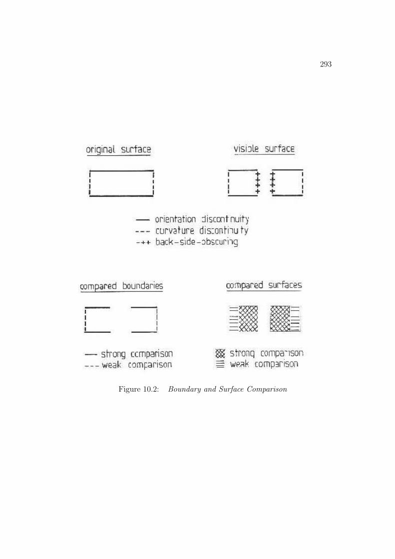
293

Figure 10.2: Boundary and Surface Comparison

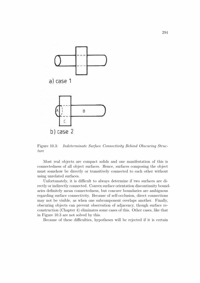
294

Figure 10.3: Indeterminate Surface Connectivity Behind Obscuring Struc-ture

Most real objects are compact solids and one manifestation of this isconnectedness of all object surfaces. Hence, surfaces composing the objectmust somehow be directly or transitively connected to each other withoutusing unrelated surfaces.

Unfortunately, it is difficult to always determine if two surfaces are di-rectly or indirectly connected. Convex surface orientation discontinuity bound-aries definitely mean connectedness, but concave boundaries are ambiguousregarding surface connectivity. Because of self-occlusion, direct connectionsmay not be visible, as when one subcomponent overlaps another. Finally,obscuring objects can prevent observation of adjacency, though surface re-construction (Chapter 4) eliminates some cases of this. Other cases, like thatin Figure 10.3 are not solved by this.

Because of these difficulties, hypotheses will be rejected if it is certain

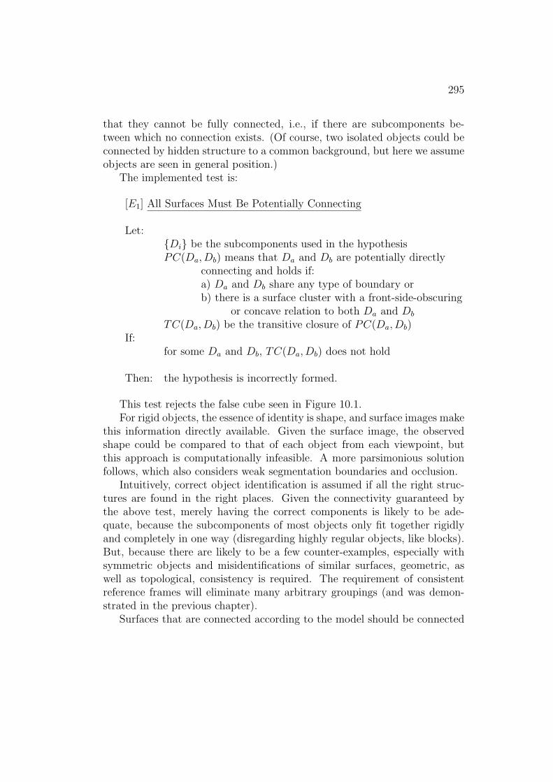
295

that they cannot be fully connected, i.e., if there are subcomponents be-tween which no connection exists. (Of course, two isolated objects could beconnected by hidden structure to a common background, but here we assumeobjects are seen in general position.)

The implemented test is:

[E1] All Surfaces Must Be Potentially Connecting

Let:{Di} be the subcomponents used in the hypothesisPC(Da, Db) means that Da and Db are potentially directly

connecting and holds if:a) Da and Db share any type of boundary orb) there is a surface cluster with a front-side-obscuring

or concave relation to both Da and Db

TC(Da, Db) be the transitive closure of PC(Da, Db)If:

for some Da and Db, TC(Da, Db) does not hold

Then: the hypothesis is incorrectly formed.

This test rejects the false cube seen in Figure 10.1.For rigid objects, the essence of identity is shape, and surface images make

this information directly available. Given the surface image, the observedshape could be compared to that of each object from each viewpoint, butthis approach is computationally infeasible. A more parsimonious solutionfollows, which also considers weak segmentation boundaries and occlusion.

Intuitively, correct object identification is assumed if all the right struc-tures are found in the right places. Given the connectivity guaranteed bythe above test, merely having the correct components is likely to be ade-quate, because the subcomponents of most objects only fit together rigidlyand completely in one way (disregarding highly regular objects, like blocks).But, because there are likely to be a few counter-examples, especially withsymmetric objects and misidentifications of similar surfaces, geometric, aswell as topological, consistency is required. The requirement of consistentreference frames will eliminate many arbitrary groupings (and was demon-strated in the previous chapter).

Surfaces that are connected according to the model should be connected

296

in the scene. This does not always imply adjacency is observable, becauseobject boundaries are not visible from all viewpoints.

Occlusion affects verification because some surfaces may be partially orcompletely missing or a surface may be broken up by closer surfaces. More-over, true surface boundaries may be obscured. The remaining true surfaceboundaries will be connected to back-side-obscuring boundaries in differentlocations. Since these are not model features, they are ignored.

Based on these ideas, the rigid object identity constraints are:

[R1] – Each data subcomponent can have at most one visible forward-facingmodel subcomponent paired with it. (The converse may not hold be-cause of fragmentation or occlusion).

[R2] – The position of observed subcomponents relative to each other is aspredicted for the corresponding model subcomponents.

[R3] – Model subcomponent adjacency implies data subcomponent adja-cency and vice versa.

These constraints were implemented as the following tests:

297

Let:{Fi} be the visible forward-facing model SURFACEs{Ii} be the image surfaces

~Pi and~P j be the predicted and observed center-of-mass for

the corresponding model and image surfaces Fi and Ij

~Ni and~N j be the predicted and observed surface orientations

at the centers-of-mass for the correspondingmodel and image surfaces Fi and Ij

τt and τr be thresholdsThen:

[R1] For each Ii there is at most one corresponding Fj.[R2] For each corresponding Ii and Fj:

| ~Pi − ~P j |< τt (τt = 20.0)

| ~Ni ◦ ~N j |> τr (τr = 0.8)

[R3] Let:Ia, Ib be two non-tangential data surfacesFa, Fb be the corresponding model SURFACEs

If:Fa and Fb are observably adjacent, Ia and Ib are not

observably adjacent, and there is no surfacecluster partially obscuring both Ia and Ib,

orFa and Fb are not observably adjacent and Ia and Ib

are observably adjacentThen: the hypothesis is incorrectly formed

Occlusion also has distinctive characteristics, and thus the hypothesis thatan object is partially or fully obscured should be subject to some verification.Back-side-obscuring boundaries usually signal this occurrence, though notalways. When a curved surface goes from facing the viewer to facing away,self-occlusion occurs without back-side-obscuring boundaries. When back-side-obscuring boundaries are present, though, three new constraints can beadded:

[O1] – the back-side-obscuring boundary should lie inside the image re-gion predicted for the SURFACE. Alternatively, the predicted image

298

Figure 10.4: Occlusion Boundaries Lie Inside Predicted Model Boundaries

boundary should lie on or outside the observed image region. Figure10.4 illustrates this.

[O2] – Back-side-obscuring boundary segments that bound the surface imageregion must end as the crossbar of a “TEE” junction. This implies thatthere must be at least three image regions at the junction. Figure 10.5illustrates this.

[O3] – A non-tangential image surface should be predicted as partially self-obscured during visibility analysis (Chapter 9) if and only if the cor-responding data surface has at least one back-side-obscuring boundarywhose closer surface is also an object surface.

Constraint O1 was not applied because parameter estimation errors madeit difficult to check this condition reliably (e.g. predicted model and data sur-faces did not overlap adequately). Constraint O2 was guaranteed assumingimage labeling was correct, which was the case here.

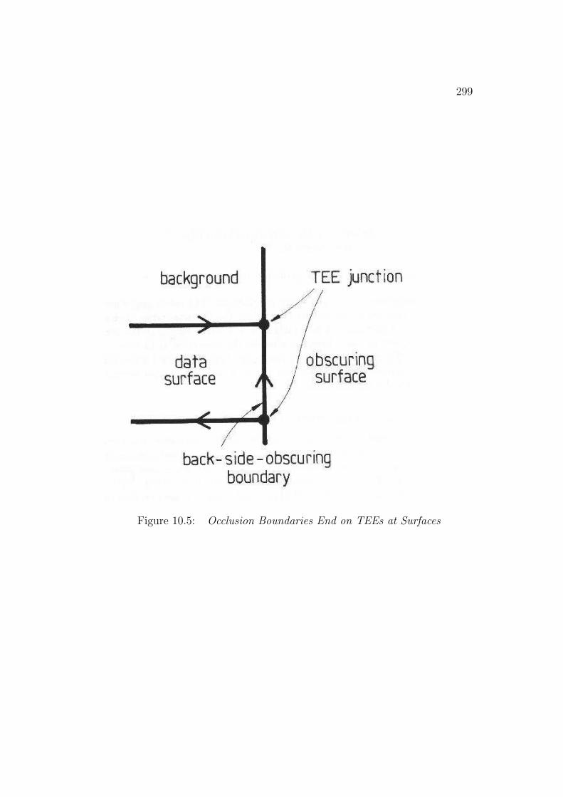
299

Figure 10.5: Occlusion Boundaries End on TEEs at Surfaces

300

Because of parameter estimation errors, it is likely that there are self-occlusions predicted during raycasting that are not observed (because of sur-faces becoming slightly obscured). Hence, the test of verifying predicted self-occlusions was not performed. While it is also possible for slightly obscureddata surfaces to be predicted as not obscured, if a self-occlusion was signifi-cant enough to be observed, then prediction was likely to show it even withparameter estimation errors. Hence, only the reverse test was implemented:

[O3] Observed Self-obscured SURFACEs Are Predicted

Let:{Di} be the non-tangential partially obscured data surfaces{Cij} be the closer data surfaces across obscuring

boundaries around Di

Si be the model SURFACE corresponding to Di

{Mk} be the other model SURFACEsfront(X,Y ) holds if model SURFACE X is directly or indirectly

in front of Y . This is found by raycasting and takingthe transitive closure.

If:For each Di and each Cij

If there is a Mk corresponding to Cij,then front(Mk, Si)

Then: the self-occlusion is as predicted by the model.

One application of O3 was particularly significant. The robot upper andlower arms are nearly symmetric, so there are two values for the upperarmposition and joint angle where the lowerarm can be nearly in the positionshown in the test scene. The difference between the two cases is whetherthe lowerarm is in front of or behind the upperarm. Though the depthsof the component reference frames are different in the two cases, parametertolerances did not completely reject the second alternative. Happily, test O3

did discriminate.

10.2.3 Non-rigidly Connected Object Verification

Non-rigidly connected object verification is trivial in comparison to the previ-ous structures. By virtue of the hypothesis construction process, all subcom-

301

ponents have been previously verified. Further, because of the coordinateframe matching process, the reference frames of the subcomponents musthave the appropriate alignment relationships with the whole ASSEMBLY.Occlusion relationships were verified by the test O3 given above. What re-mains is to verify that the variable joint parameters meet any given con-straints. These are constrained using the general method given in the nextsubsection.

10.2.4 Numerical Constraint Evaluation

Many numerical values are associated with hypotheses. The most importantof these are the property values described in Chapter 6, but there could alsobe other values such as the object position or joint angles. Constraints can bespecified on these values and they must hold for the verification to succeed.

The constraints were mainly used for eliminating spurious SURFACEhypotheses and usually tested absolute surface area.

The constraints are specified as part of the model definition process, as aset of statements of the form:

CONSTRAINT < name > < constraint >

The < constraint > must apply in the context of structure < name >.Here:

< constraint > ::= < pconstraint >|< constraint > AND < constraint >|< constraint > OR < constraint >|(< constraint >)

< pconstraint > ::= < value >< relation >< number >< relation > ::= <|>|=|<=|>=| !=< value > ::= < variable >|< property >(< name >)

The < value > refers to a variable or a property (possibly of a substruc-ture) in the context of the structure being constrained. Other constraint ex-pressions could have been easily added. The verification of these constraintsis trivial.

An example of such a constraint for the elbow joint angle jnt3 in the robotarmasm ASSEMBLY is:

CONSTRAINT armasm (jnt3 < 2.5) OR (jnt3 > 3.78);

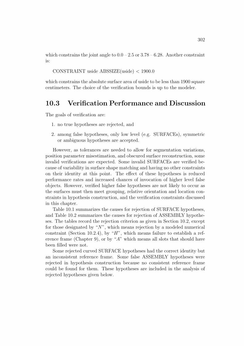
302

which constrains the joint angle to 0.0 – 2.5 or 3.78 – 6.28. Another constraintis:

CONSTRAINT uside ABSSIZE(uside) < 1900.0

which constrains the absolute surface area of uside to be less than 1900 squarecentimeters. The choice of the verification bounds is up to the modeler.

10.3 Verification Performance and Discussion

The goals of verification are:

1. no true hypotheses are rejected, and

2. among false hypotheses, only low level (e.g. SURFACEs), symmetricor ambiguous hypotheses are accepted.

However, as tolerances are needed to allow for segmentation variations,position parameter misestimation, and obscured surface reconstruction, someinvalid verifications are expected. Some invalid SURFACEs are verified be-cause of variability in surface shape matching and having no other constraintson their identity at this point. The effect of these hypotheses is reducedperformance rates and increased chances of invocation of higher level falseobjects. However, verified higher false hypotheses are not likely to occur asthe surfaces must then meet grouping, relative orientation and location con-straints in hypothesis construction, and the verification constraints discussedin this chapter.

Table 10.1 summarizes the causes for rejection of SURFACE hypotheses,and Table 10.2 summarizes the causes for rejection of ASSEMBLY hypothe-ses. The tables record the rejection criterion as given in Section 10.2, exceptfor those designated by “N”, which means rejection by a modeled numericalconstraint (Section 10.2.4), by “H”, which means failure to establish a ref-erence frame (Chapter 9), or by “A” which means all slots that should havebeen filled were not.

Some rejected curved SURFACE hypotheses had the correct identity butan inconsistent reference frame. Some false ASSEMBLY hypotheses wererejected in hypothesis construction because no consistent reference framecould be found for them. These hypotheses are included in the analysis ofrejected hypotheses given below.

303

Table 10.1: SURFACE Hypothesis Rejection Summary

IMAGE REJECTION

SURFACE REGIONS RULE INSTANCES

uedgeb 19,22 N 2

lsidea 19,22 N 1

lsideb 19,22 N 1

robbodyside 9 N 4

robbodyside 8 S2 2

robshould1 12 S2 1

robshould2 12 S2 1

robshoulds 27 S2 2

tcaninf 9 S2 2

Table 10.3 lists and analyzes all remaining verified hypotheses that werenot “correct”. The most common causes of incorrectly verified hypotheseswere symmetric models, leading to multiple reference frames, and nearlyidentical models. The incorrect models normally were not used in largerASSEMBLYs, because of reference frame inconsistencies.

These results show that verification worked well. Two true ASSEMBLYhypotheses were rejected because of deficiencies in geometric reasoning. Allverified false hypotheses were reasonable, usually arising from either a simi-lar or symmetric object model. Most rejected SURFACE hypotheses failedthe value constraint (usually surface area – see Appendix A). Curved SUR-FACEs were rejected when their curvature axis was inconsistent with otherorientation estimates. Most ASSEMBLYs were rejected because no consis-tent reference frame could be found. (Many of these hypotheses arose becausehypothesis construction has a combinatorial aspect during initial hypothesisconstruction.)

304

Table 10.2: ASSEMBLY Hypothesis Rejection Summary

IMAGE REJECTION

ASSEMBLY REGIONS RULE INSTANCES NOTE

lowerarm 12,18,31 H 30

lowerarm 17,19,22, A 1

25,32

lowerarm 17,19,22, H 1

25,32

upperarm 17,19,22, H 6

25,32

armasm 12,17,18, R3 2

19,22,25

31,32

armasm 12,17,18, O3 1

19,22,25

31,32

robshldbd 16,26 H 3

robshldsobj 29 H 1 +1

robbody all appt. H 3 +1

robot all appt. H 5

+1 valid hypothesis rejection because of geometric reasoning error

305

Table 10.3: Incorrectly Verified Hypotheses Analyzed

MODEL TRUE IMAGE

USED MODEL REGIONS NOTE

uside uside 19,22 +3

uends uends 25 +2

lsidea lsideb 12 +1

lsideb lsideb 12 +2

ledgea ledgea 18 +2

ledgeb ledgea 18 +1

lendb lendb 25 +2

robbodyside robbodyside 8 +2

robshould1 robshould2 16 +1

robshould2 robshould2 16 +2

lowerarm lowerarm 12,18,31 +2

upperarm upperarm 17,19,22, +2

25,32

robbody robbody 8 +2

trashcan trashcan 9,28,38 +2

+1 true model similar to invoked model+2 symmetric model gives match with another reference frame+3 error because substantially obscured

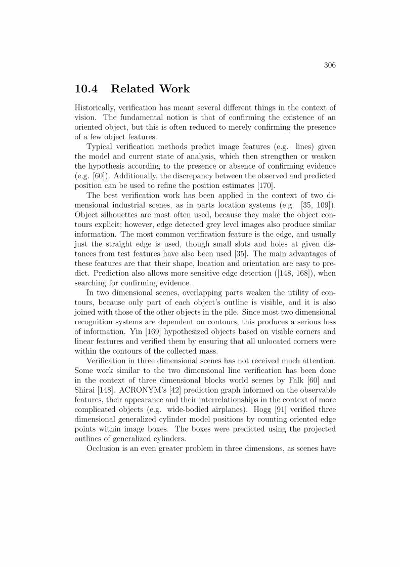
306

10.4 Related Work

Historically, verification has meant several different things in the context ofvision. The fundamental notion is that of confirming the existence of anoriented object, but this is often reduced to merely confirming the presenceof a few object features.

Typical verification methods predict image features (e.g. lines) giventhe model and current state of analysis, which then strengthen or weakenthe hypothesis according to the presence or absence of confirming evidence(e.g. [60]). Additionally, the discrepancy between the observed and predictedposition can be used to refine the position estimates [170].

The best verification work has been applied in the context of two di-mensional industrial scenes, as in parts location systems (e.g. [35, 109]).Object silhouettes are most often used, because they make the object con-tours explicit; however, edge detected grey level images also produce similarinformation. The most common verification feature is the edge, and usuallyjust the straight edge is used, though small slots and holes at given dis-tances from test features have also been used [35]. The main advantages ofthese features are that their shape, location and orientation are easy to pre-dict. Prediction also allows more sensitive edge detection ([148, 168]), whensearching for confirming evidence.

In two dimensional scenes, overlapping parts weaken the utility of con-tours, because only part of each object’s outline is visible, and it is alsojoined with those of the other objects in the pile. Since most two dimensionalrecognition systems are dependent on contours, this produces a serious lossof information. Yin [169] hypothesized objects based on visible corners andlinear features and verified them by ensuring that all unlocated corners werewithin the contours of the collected mass.

Verification in three dimensional scenes has not received much attention.Some work similar to the two dimensional line verification has been donein the context of three dimensional blocks world scenes by Falk [60] andShirai [148]. ACRONYM’s [42] prediction graph informed on the observablefeatures, their appearance and their interrelationships in the context of morecomplicated objects (e.g. wide-bodied airplanes). Hogg [91] verified threedimensional generalized cylinder model positions by counting oriented edgepoints within image boxes. The boxes were predicted using the projectedoutlines of generalized cylinders.

Occlusion is an even greater problem in three dimensions, as scenes have

307

natural depth and hence objects will often self-obscure as well as obscureeach other. Brooks [42] suggested that a model-based geometric reasoningvision system could predict what features will be self-obscured from a givenviewpoint. In the context of the blocks world scene analysis, occlusion hy-potheses were verified by detecting single TEE junctions to signal the startof occlusion (e.g. [162]) and pairs of TEEs indicated which edges should beassociated (e.g. [80]).

10.5 Discussion

The most important deficiency of verification is its approach to identity. Forverification, objects are probably more suitably represented by listing desir-able and undesirable properties, rather than an exact geometric model, es-pecially as verification thoroughness is probably proportional to the individ-uality of the object and the degree of generic identification desired. Humanfaces need detailed shape comparisons for precise identification, but just tosay it was human requires less. On the other hand, chairs have a tremendousvariety of shapes, but there is no prototype chair model, even given divisioninto functional groupings. If the only common factors were support for backand seat at given heights, sizes and orientations, then a pile of boxes wouldalso be satisfactory, and this may not always be an appropriate identification.

One key benefit of the approach described in this chapter is that the spe-cific verification criteria are linked to the geometric model, which promotesmore general applicability.

There is some overlap between the functions of hypothesis construction(Chapter 9) and verification. The construction and verification sequence fol-lows the classical Artificial Intelligence “generate and test” paradigm. Thegoal of the construction process is to: (1) find evidence for all model featuresand (2) assign a reference frame. To prevent (1) from causing a combinatorialexplosion, some constraints were applied when searching for image evidence.On the other hand, verification ensures that the whole object satisfies allconstraints, including some previously applied. Hence, there could be someshifting of constraint analysis to verification, particularly if hypothesis con-struction and verification became more of a parallel process (i.e. akin to aWaltz filtering process [162]).

Verification of partially obscured or partially back-facing SURFACEs isweak. For these SURFACEs, only individual summary characteristics were

308

Figure 10.6: Partially Obscured Square Verification

checked, leaving other tests until the SURFACE was combined with othersin an ASSEMBLY. More detailed symbolic comparisons could be made, as inFigure 10.6. Here, a square is somewhat obscured. Verification could easilyshow that it was not a circle, and that it is likely to be a square, by com-paring descriptions of the boundary. This technique could also be used forthe full and partial boundary comparisons, as proposed above, because com-paring symbolic descriptions is faster and easier than creating the predictedboundary path.

More practical constraints will be needed for richer object domains, par-ticularly for natural objects, where within-class variation presents problems.This is apparent with faces, whose shape changes between people and ex-pressions. This research allowed some variation by using only approximatecurvature and position in constraints (S2 and R2), but this is weak and maynot generalize properly. Further, flexible surfaces will also have variable seg-mentation, which will lead to difficulties with constraints based on curvatureor correspondence.

Final Comments

To summarize, this chapter extended verification to cover fully visible andpartially obscured SURFACEs and ASSEMBLYs in three dimensional scenes.

309

This required understanding how object location, external occlusion and self-occlusion affect appearance. Constraints that helped guarantee the existenceand identity of the modeled objects were formulated and demonstrated.

Chapter 11

Discussion and Conclusions

This book has described an Artificial Intelligence approach to the problemof three dimensional object recognition, based on methods that lead to gen-eral purpose vision systems rather than to limited single application systems.While efficiency is ultimately important, competence must come first. Onlya few researchers have used 21

2D sketch-like surface data, and the work de-

scribed here has attempted to explore the whole path from surfaces to objects.The structure of the approach mirrors classical edge-based recognition pro-cesses, but the use of surface data required new definitions of the processesand their interconnections.

Some of the interesting aspects of the individual recognition processeswere:

1. object modeling

• a surface modeling method based on distinct curvature class patches.

• criteria for how to group model SURFACEs into ASSEMBLYs.

2. surface data

• proposed criteria for segmentation of surface image data into sur-face patches useful for object recognition.

3. surface hypothesizing

• analysis of surface occlusion cases to show what cases occur, howto detect them and how to hypothetically reconstruct the missingdata. Because the research used three dimensional surface image

310

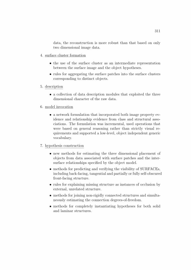
311

data, the reconstruction is more robust than that based on onlytwo dimensional image data.

4. surface cluster formation

• the use of the surface cluster as an intermediate representationbetween the surface image and the object hypotheses.

• rules for aggregating the surface patches into the surface clusterscorresponding to distinct objects.

5. description

• a collection of data description modules that exploited the threedimensional character of the raw data.

6. model invocation

• a network formulation that incorporated both image property ev-idence and relationship evidence from class and structural asso-ciations. The formulation was incremental, used operations thatwere based on general reasoning rather than strictly visual re-quirements and supported a low-level, object independent genericvocabulary.

7. hypothesis construction

• new methods for estimating the three dimensional placement ofobjects from data associated with surface patches and the inter-surface relationships specified by the object model.

• methods for predicting and verifying the visibility of SURFACEs,including back-facing, tangential and partially or fully self-obscuredfront-facing structure.

• rules for explaining missing structure as instances of occlusion byexternal, unrelated structure.

• methods for joining non-rigidly connected structures and simulta-neously estimating the connection degrees-of-freedom.

• methods for completely instantiating hypotheses for both solidand laminar structures.

312

8. verification

• criteria for verifying the physical existence of a hypothesis.

• criteria for verifying the identity of an object based on surfaceevidence.

The research also emphasized the strong distinction between, but equallystrong dependence on, the suggestive “seeing” of model invocation and themodel-directed hypothesis construction and verification. Finally, the effectof occlusion was considered throughout the visual process, and methods weredeveloped that helped overcome data loss at each stage.

When applying the recognition processes described in this book to the(hand) segmented range image shown in Figure 3.10, the IMAGINE I sys-tem correctly recognized all modeled objects in the test scene (the robotand trash can, and their subcomponents). No misidentifications of solidsoccurred, though several individual surfaces were misidentified. Since themodel base included 16 ASSEMBLYs, all of about the same size, includ-ing several objects not in this scene (a chair and its subcomponents), thiswas a good result. The original geometric reasoning module gave decent,but not ideal position and joint angle estimation (seen in Figure 9.16) and anew network-based geometric reasoning method improved on this (see Figure1.11).

Three test scenes were analyzed. The one used in this book was themost interesting, because it contained articulated objects with some curvedsurfaces, laminar surfaced objects, partially constrained degrees-of-freedom(joints) and considerable self-occlusion.

The success of the recognition process was largely because of the richnessof the 21

2D sketch data, but the use of the surface-based hierarchical mod-

els, shape segmented surface patches and hierarchical surface cluster datarepresentation made the results easier to obtain.

This recognition process was clearly successful on the test image. How-ever, much research is still needed, and the following section tries to makeexplicit some of the problems that remain. I welcome others to add to thelist and to solve them all.

313

11.1 Summary of Outstanding Problems

Input Data

The data used in this research were unrealistic in several respects. Be-cause the depth and orientation values and the segmentation boundaries werehand-derived, they had few of the errors likely to be present in real data. Thesegmentations also made nearly perfect correspondence with the models, andthus ignored problems of data variation and scale. Data variations, particu-larly for objects with curved surfaces, cause shape segmentation boundariesto shift. Further, as the analytic scale changes, segmentation boundaries alsomove, and segments may appear or disappear.

Object Modeling

The object representation was too literal and should not always be basedon exact sizes and feature placement. The object surfaces could be morenotional, designating surface class, curvature, orientation and placement andlargely ignore extent. Object representation could also have a more concep-tual character that emphasizes key distinguishing features and rough geo-metric placement, without a literal CAD-like model (as used here). Finally,the models could allow alternative, overlapping representations, such as hav-ing two surfaces used individually and as part of a connecting orientationdiscontinuity.

As data occurs at unpredictable scales, the models might record the fea-tures at a variety of scales. The models should also include other data el-ements such as references to solids (e.g. generalized cylinders), reflectance,surface shape texture and distinguished axes (e.g. symmetry and elongation),etc. The representation could have used a more constraint-like formulation,as in ACRONYM [42], which would allow inequality relationships amongfeatures, and also allow easier use of model variables. Many of these inade-quacies were subsequently overcome in the SMS representation approach [70]described in Chapter 7.

Surface Reconstruction

314

An open question about the surface reconstruction process is whetherto replace the representation of two partially obscured surfaces by a singlemerged surface (as was done) or to keep both alternatives. Keeping the extrahypotheses causes redundant processing and may lead to duplicated invoca-tion and hypothesis construction, but allows correct processing if the mergingwas inappropriate. Keeping only the merged surface may cause invocationand matching failures, or require a more intelligent hypothesis constructionprocess that uses the model to decide if the two surfaces were incorrectlymerged.

Surface Cluster Formation

The surface cluster formation process has a similar problem. When onesurface cluster overlaps another, then a third surface cluster merging the twois created as well. This was to provide a context within which all componentsof a self-obscured object would appear. The problem is how to control thesurface cluster merging process when multiple surface clusters overlap (as islikely in a real scene), which causes a combinatorial growth of surface clusters.

Data Description

While shape is very informative, many additional description types couldbe added to help characterize objects: reflectance and shape texture (bothrandom and patterned), reflectance itself, translucency, surface finish, etc.

Model Invocation

Invocation evaluated a copy of the network in every image context. Thisis computationally expensive, considering the likely number of contexts (e.g.100) and the number of models (e.g. 50,000) in a realistic scene. Parallelprocessing may completely eliminate the computational problem, but thereremains the problem of investigating just the relevant contexts. There shouldprobably be a partitioning of the models according to the size of the context,and also some attention focusing mechanism should limit the context within

315

which invocation takes place. This mechanism might apply a rough high-level description of the entire scene and then a coarse-to-fine scale analysisfocusing attention to particular regions of interest.

Redundant processing might arise because an object will invoke all ofits generalizations. The invocations are correct, but the duplication of effortseems wasteful when a direct method could then pursue models up and downthe generalization hierarchy.

As currently formulated, the invocation network must be created sym-bolically for each new scene analyzed, as a function of the scene, model baseand evidence computations. It would be interesting to investigate how thenetwork might re-organize itself as the image changed, maintaining the fixedmodel dependent relationships, but varying the image dependent ones.

The variety of objects in the natural word suggests that there may notbe a “rich” description hierarchy, nor a deep subcomponent hierarchy formost objects, nor a general subclass hierarchy. Though these factors con-tribute substantially, it appears that there are relatively few object types inour everyday experience. Instead, there are many individuals and consid-erable variation between individuals. Thus, the most important aspect ofobject representation may be the direct property and primitive descriptionevidences, which would then differentiate individuals.

Hypothesis Construction

The major criticism of the hypothesis construction process is its literality.In particular, it tried to find evidence for all features, which is probablyneither fully necessary, nor always possible.

Literality also appeared in the dependence on the metrical relationshipsin the geometric model (e.g. the surface sizes and boundary placements).These were used for predicting self-occlusion and for spatially registering theobject. While these tasks are important, and are part of a general vision sys-tem, they should have a more conceptual and less analytic formulation. Thiswould provide a stronger symbolic aspect to the computation and should alsomake the process more capable of handling imperfect or generic objects.

The Recognition Approach as a Whole

316

One significant limitation of the recognition approach is the absence ofscale analysis. Objects should have different conceptual descriptions accord-ing to the relevance of a feature at a given scale, and recognition then has tomatch data within a scale-dependent range of models.

A more relational formulation would help, but there does not seem tobe a matching method that neatly combines the tidiness and theoreticalstrengths of graph matching with the efficiency and prediction capability ofmodel-based geometric matching.

The proposed recognition model ignored the question of when enoughevidence was accumulated. Recognition need not require complete evidenceor satisfaction of all constraints, provided none actually fail, and the few ob-served features are adequate for unique identification in a particular context.However, the implementation here plodded along trying to find as much ev-idence as possible. An object should be recognizable using a minimal setof discriminating features and, provided the set of descriptions is powerfulenough to discriminate in a large domain, the recognition process will avoidexcessive simplification. Recognition (here) has no concept of context, andso cannot make these simplifications. On the other hand, the additional ev-idence provides the redundancy needed to overcome data and segmentationerrors.

The evaluation on hand-collected and segmented data did not adequatelytest the methods, but research using this approach is continuing and somesimpler genuine range data scenes have been successfully analyzed.

11.2 The IMAGINE II System

Experience with the IMAGINE I program has led to a redesign embodiedin the IMAGINE II system. Though the re-implementation is not com-plete, the design of the system and its key representations and processes aresummarized here. Figure 11.1 shows a block diagram of the main modules ofthe IMAGINE II system. The system is intended to interpret data derivingfrom scenes containing self and externally obscured complex, non-polyhedralman-made objects including possible degrees-of-freedom (e.g. robot joints).

As in IMAGINE I, data comes from a segmented 212D sketch, except

that curve and volumetric scene features may be part of the input, too. Thedata may be fragmented or incomplete. The input data structure is a REV(Region, Edge, Vertex) graph. The system output is, as before, a list of

317

object hypotheses with position and parameter estimates and a set of imageevidence and justifications supporting the object hypothesis.

Building the VSCP Structure

The first new representation is the VSCP structure (Volume, Surface,Curve, Point), which is constructed from the REV by knowledge-based struc-ture completion processes. The goal of this process is to group curve and sur-face features from the REV to overcome fragmentation and occlusion effectsand to remove non-structural artifacts (e.g. reflectance edges). The originalraw data might be interrogated to help verify deductions.

An example of an occlusion rule is:

• If two valid TEE junctions lying on the boundary of the same surfacecan be extended (using the local boundary shape) until they intersect,and the curve extensions lie behind closer surfaces, then hypothesizethat the original shape of the partially obscured surface is that of theextended surface.

An example of a fragmentation rule is:

• If two surface patches are “adjacent”, have similar shape, depth andorientation and there are not intervening space curves (e.g. from patchedges or closer surfaces), then merge the two patches.

Here “adjacent” is a heuristic concept because the surface characterization isassumed to be neither complete nor dense (i.e. there may be missing surfacesand there might be substantial gaps between nearby patches).

Building the Contexts Structure

Invocation and matching occur in data contexts, only now contexts existfor curves and volumes as well as surfaces and surface clusters. Contextsimprove matching efficiency by grouping related data and thereby isolatingirrelevant data, and create a structure that can accumulate plausibility formodel invocation.

The context structures are hierarchical in that contexts can be groupedto form larger contexts. Contexts are designed to support recognition of

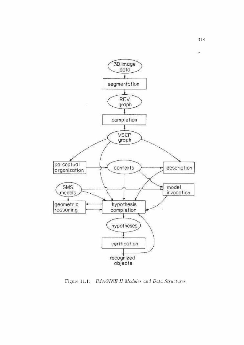
318

Figure 11.1: IMAGINE II Modules and Data Structures

319

curves, surfaces, volumes and larger groupings of features. For example, theinformation contained in a surface context might link to both curve fragmentsand surface patches, because either might help define a complete surface.

Examples of context-forming rules are:

• If a set of adjacent surface patches are completely isolated by depthdiscontinuity boundaries and there are no such boundaries internal tothe group, then these surfaces form a context for recognizing an AS-SEMBLY.

• If a set of space curves roughly surrounds a region of two dimensionalimage space and the curves are not radically different in depth, thenhypothesize that a surface context lies within the curves.

Structure Description

Model invocation and hypothesis construction require property estimatesfor image features, and because we are using 2 1/2D sketch data, three di-mensional properties can be directly measured. These properties are similarto those used for IMAGINE I (Chapter 6), and include:

• curve fragment properties: length, curvature, ...

• surface fragment properties: area, curvature, elongation, ...

• curve fragment pairs: relative orientation, relative size, ...

• surface fragment pairs: relative orientation, relative size, ...

Model Invocation

Model invocation is nearly the same as in IMAGINE I (Chapter 8).A network implements the computation in a manner suitable for parallelevaluation. Nodes represent the pairing between individual model and datafeatures, and are connected to other nodes according to the type of relation.Relations include: structural (e.g. “subcomponent of”), generic (e.g. “visualspecialization of”), class (e.g. “non-visual specialization of”), inhibiting andgeneral association. Direct evidence comes from a measure of the fit between

320

data and model properties.

Object Models

The SMS models are used, as described in Chapter 7. They are primarilystructural with model primitives designed to match with either curve, surfaceor volumetric data as alternatives. The models are hierarchical, buildinglarger models from previously defined substructures. All model dimensionsand reference frame transformations may involve variables and expressions,and algebraic constraints can bound the range of the variables.

The models have viewpoint dependent feature groups, which record thefundamentally distinct viewpoints of the object. They also identify (1) modelfeatures visible from the viewpoint and (2) new viewpoint dependent features(such as occlusion relationships, TEE junctions or extremal boundaries).

Hypothesis Construction

Initial selection of the model may come bottom-up from invocation ortop-down as part of another hypothesis being constructed. Hypothesis con-struction then attempts to find evidence for all model features.

Feature visibility information comes from a viewpoint dependent featuregroup, which is selected according to the estimated orientation of the object.

Construction is largely hierarchical, grouping recognized subcomponentsto form larger hypotheses. The most primitive features are designed to berecognized using either curve, surface or volumetric data, depending on whatis available. At all stages, geometric consistency is required, which also re-sults in more precise position estimates and estimates for embedded variables(such as a variable rotation angle about an axis).

Construction is a heuristic process whereby various approaches are triedto find evidence for a feature. For example, some heuristics for surface findingare:

1. Use an image patch if it has the predicted position, orientation, shapeand size.

2. Use a smaller image patch if it has the predicted position, orienta-tion and shape and no patch of the correct size is found (i.e. accept

321

fragmented patches).

3. Do not look for the surface if it is small and far away.

Application of the heuristics is controlled through routines that know whatapproaches are available for finding features (and when to try them) and hassomewhat of an “expert system” character.

Geometric Reasoning

The network-based geometric reasoning was described in Section 9.2.4.The geometric relationships between model features, model and data pair-ings and a priori scene knowledge are represented algebraically and are im-plemented as networks expressing the computational relationships betweenthe variables.

Analysis of the types of geometric relationships occurring in scene anal-ysis showed that most relationships could be expressed using only a smallset of standard relationships (e.g. “a model point is paired with a datapoint”). The standard relationships are then be used to create standardnetwork modules, which are allocated and connected as model matching pro-duces new model-to-data pairings.

Agenda Management

To facilitate experimentation with different control regimes, the hypothe-sis construction processes are activated from a priority-ordered agenda. Theprocesses take inputs from and return results to a global blackboard. Anagenda item embodies a request for applying a specified hypothesis con-struction process on a given datum or hypothesis. The activated process maythen enter other requests into the agenda. We use the agenda to implementa mixed control regime involving both top-down and bottom-up hypothesisconstruction.

Hypothesis Verification

322

Because data can be fragmented or erroneous, object hypotheses may beincomplete. Further, spurious hypotheses may be created from coincidentalalignments between scene features. Hypothesis construction and geometricreasoning eliminate some spurious hypotheses, but other instances of globalinconsistency may remain.

This module considers two problems: (1) global consistency of evidence(e.g. connectedness and proper depth ordering of all components) and (2)heuristic criteria for when to accept incomplete models.

11.3 Conclusion

This concludes our description of the IMAGINE I vision system. Startingfrom surface depth and orientation information for the visible surfaces in thescene, it could:

• produce an identity-independent segmentation of the objects in thescene,

• describe their three dimensional properties,

• select models to explain the image data,

• methodically pair the data to model features (while extracting the ob-ject’s spatial position and explaining missing features arising from oc-clusion or object position) and

• verify the existence and identity of the instantiated hypotheses

for non-polyhedral solids, laminar structures and non-rigidly connected struc-tures, without sacrificing a detailed understanding of the objects or theirrelationships to the scene.

Three dimensional object recognition is obviously a complex problem, andthis research has attempted to address many issues. A skeletal explorationseemed appropriate because the use of surface data for recognition was andstill is relatively untried. Thus, examining the whole problem exposed manyareas for future research, some of which are being investigated as IMAGINEII is being developed. Consequently, the results presented have not solvedthe problem of three dimensional scene understanding, but they are a fewmore steps on the way.

323

The following abbreviations are used:

ANCAI - American National Conference on Artificial IntelligenceIJCAI - International Joint Conference on Artificial IntelligenceSRI - Stanford Research Institute

Bibliography

[1] Abe, N., Itho, F., Tsuji, S., Toward Generation of 3-DimensionalModels of Objects Using 2-Dimensional Figures and Explanationsin Language, Proceedings 8th IJCAI, pp1113-1115, 1983.

[2] Ackley, D., Hinton, G., Sejnowski, T., A Learning Algorithm forBoltzmann Machines, Cognitive Science, Vol 9, pp147-169, 1985.

[3] Adler, M., Understanding Peanuts Cartoons, Department of Ar-tificial Intelligence Research Report 13, University of Edinburgh,1975.

[4] Adorni, G., Trucco, E., A Quantitative Theory of Vi-sual Perception: A Case Study, in Cappellini and Marconi (eds),Advances in ImageProcessing and Pattern Recognition, pp 130-138, North Holland,Amsterdam, 1986.

[5] Agin, G. J., Binford, T. O., Computer Description of Curved Ob-jects, Proceedings 3rd IJCAI, pp629-640, 1973.

[6] Agin, G. J., Hierarchical Representation of Three-DimensionalObjects Using Verbal Models, SRI Technical Note 182, 1979.

[7] Alefeld, G., Herzberger, J., Introduction to Interval Computations,Academic Press, New York, 1983.

[8] Ambler, A. P., Barrow, H. G., Brown, C. M., Burstall, R. M.,Popplestone, R. J., A Versatile System for Computer ControlledAssembly, Artificial Intelligence, Vol. 6, pp129 - 156, 1975.

324

325

[9] Arbib, M. A., Local Organizing Processes and Motion Schemas inVisual Perception, in Hayes, et al. (eds), Machine Intelligence 9,pp287-298, Ellis-Horwood, Chichester, 1979.

[10] Asada, H., Brady, M., The Curvature Primal Sketch, Mas-sachusetts Institute of Technology AI memo 758, 1984.

[11] Aylett, J. C., Fisher, R. B., Fothergill, A. P., Predictive ComputerVision for Robotic Assembly, Journal of Intelligent and RoboticSystems, Vol. 1, pp185-201, 1988.

[12] Ballard, D. H., Parameter Networks: Towards a Theory of Low-Level Vision, Proceedings 7th IJCAI, pp1068-1078, 1981.

[13] Ballard, D. H., Sabbah, D., On Shapes, Proceedings 7th IJCAI,pp607-612, 1981.

[14] Ballard, D. H., Brown, C. M., Computer Vision, Prentice-Hall,New Jersey, 1982.

[15] Ballard, D. H., Tanaka, H., Transformational Form Perception in3D: Constraints, Algorithms, Implementations, Proceedings 9thIJCAI, pp964-968, 1985.

[16] Barrow, H. G., Popplestone, R. J., Relational Descrip-tions in Picture Processing, in Meltzer and Michie (eds),Machine Intelligence 6, pp377-396, Edinburgh University Press,Edinburgh, 1971.

[17] Barrow, H. G., Ambler, A. P., Burstall, R. M., Some Tech-niques for Recognizing Structures in Pictures, in Watanabe (ed.)Frontiers of Pattern Recognition, pp1-29, Academic Press, NewYork, 1972.

[18] Barrow, H. G., Burstall, R. M., Subgraph Isomorphism, MatchingRelational Structures and Maximal Cliques, University of Edin-burgh, Department of Artificial Intelligence, Working Paper 5,Nov 1974.

[19] Barrow, H. G., Tenenbaum, J. M., MSYS: a System for ReasoningAbout Scenes, SRI Technical Note 121, 1976.

326

[20] Barrow, H. G., Tenenbaum, J. M., Recovering Intrinsic SceneCharacteristics from Images, in Hanson and Riseman (eds),Computer VisionSystems, pp3-26, Academic Press, New York, 1978.

[21] Barnard, S. T., Pentland, A. P., Three-Dimensional Shape fromLine Drawing, Proceedings 8th IJCAI, pp1062-1064, 1983.

[22] Berthod, M., Global Optimization of a Consistent Labeling, Pro-ceedings 8th IJCAI, pp1065-1067, 1983.

[23] Besl, P. J., Jain, R. C., Three Dimensional Object Recognition,Association for Computing Machinery Computing Surveys, Vol17, pp 75-145, 1985.

[24] Besl, P. J., Surfaces in Early Range Image Understanding, PhDDissertation, Electrical Engineering and Computer Science De-partment (RSD-TR-10-86), University of Michigan, 1986.

[25] Besl, P. J., Range Imaging Sensors, General Motors ResearchPublication GMR-6090, General Motors Research Laboratories,Warren, Michigan, 1988.

[26] Besl, P. J., Geometric Modelling and Computer Vision, GeneralMotors Research Publication GMR-6248, General Motors Re-search Laboratories, Warren, Michigan, 1988.

[27] Binford, T. O., Visual Perception by Computer, IEEE Conferenceon Systems and Control, 1981.

[28] Binford, T. O., Inferring Surfaces from Images, Artificial Intelli-gence, Vol. 17, pp205-244, 1981.

[29] Binford, T. O., Survey of Model-Based Image Analysis Systems,International Journal of Robotics Research, Vol 1, pp18-64, 1982.

[30] Binford, T. O., Levitt, T. S., Mann, W. B., Bayesian Inference inModel-Based Machine Vision, unpublished note, Computer Sci-ence, Stanford University, 1987.

[31] Blake, A., Reconstructing a Visible Surface, Proceedings 3rd AN-CAI, pp23-26, 1984.

327

[32] Blake, A., Specular Stereo, Proceedings 9th IJCAI, pp 973-976,1985.

[33] Bledsoe, W. W., A new method for proving certain Presburgerformulas, Proceedings 4th IJCAI, pp15-21, 1975.

[34] Boissonnat, J. D., Faugeras, O. D., Triangulation of 3D Objects,Proceedings 7th IJCAI, pp658-660, 1981.

[35] Bolles, R., Locating Partially Visible Objects: The Local FeatureFocus Method, ANCAI 80 and SRI Technical Note 223, Aug 1980.

[36] Bolles, R.C., Horaud, P., Hannah, M. J., 3DPO: a Three-Dimensional Part Orientation System, Proceedings 8th IJCAI,pp1116-1120, 1983.

[37] Boyer, K. L., Kak, A. C., Color encoded structured light for rapidactive ranging, IEEE Transactions on Pattern Analysis and Ma-chine Intelligence, Vol 9, pp 14-28, 1987.

[38] Brady, M., Yuille, A., An Extremum Principle for Shape fromContour, Proceedings 8th IJCAI, pp969-972, 1983.

[39] Brady, M., Criteria for Representations of Shape, in Beck,Hope and Rosenfeld (eds), Human and Machine Vision, Aca-demic Press, London, 1983.

[40] Brady, M., Ponce, J., Yuille, A., Asada, H., Describing Surfaces,Proceedings 2nd International Symp. on Robotics Research, 1984.

[41] Brice, C. R., Fennema, C. L., Scene Analysis Using Regions, Ar-tificial Intelligence, Vol. 1, pp205-226, 1970.

[42] Brooks, R. A., Symbolic Reasoning Among 3D Models and 2DImages, Stanford AIM-343, STAN-CS-81-861, 1981.

[43] Cai, L. D., Forthcoming PhD Thesis, Department of ArtificialIntelligence, University of Edinburgh, 1989.

[44] Cameron, S. A., Modelling Solids in Motion, PhD Thesis, Depart-ment of Artificial Intelligence, University of Edinburgh, 1984.

328

[45] Cernuschi-Frias, B., Bolle, R. M., Cooper, D. B., A New Concep-tually Attractive & Computationally Effective Approach to Shapefrom Shading, Proceedings 8th IJCAI, pp966-968, 1983.

[46] Chang, N. S., Fu, K. S., Parallel Parsing of Tree Languages forSyntactic Pattern Recognition, Pattern Recognition, Vol 11, page213, 1979.

[47] Chakravarty, I., The use of characteristic views as a basis forrecognition of three dimensional objects, IPL-TR-034, Image Pro-cessing Laboratory, Rensselaer Polytechnic Institute, 1982.

[48] Clowes, M. B., On Seeing Things, Artificial Intelligence, Vol. 2,pp79-116, 1971.

[49] Clocksin, W., The Effect of Motion Contrast on Surface Slantand Edge Detection, Proceedings British Society for the Study ofArtificial Intelligence and the Simulation of Behaviour Conference,1980.

[50] Coleman, E. N., Jain, R., Shape from Shading for Surfaces WithTexture and Specularity, Proceedings 7th IJCAI, pp652-657, 1981.

[51] Cowie, R. I. D., The Viewer’s Place in Theories of Vision, Pro-ceedings 8th IJCAI, pp952-958, 1983.

[52] Dane, C., Bajcsy, R., An Object-Centered Three DimensionalModel Builder, Proceedings 6th International Conference on Pat-tern Recognition, pp348-350, 1982.

[53] Davis, E., Constraint Propagation with Interval Labels, ArtificialIntelligence, Vol 32, p281, 1987.

[54] Dreschler, L., Nagel, H. H., Volumetric Model and 3D-Trajectoryof a Moving Car Derived from Monocular TV-frame Sequences ofa Street Scene, Proceedings 7th IJCAI, pp692-697, 1981.

[55] Duda, R., Hart, P., Experiments in Scene Analysis, SRI ArtificialIntelligence Group Technical note 20, Project 8259, Jan 1970.

[56] Duda, R., Hart, P., Pattern Classification and Scene Analysis,John Wiley and Sons, New York, 1973.

329

[57] Durrant-Whyte, H. F., Uncertain geometry in robotics, Proceed-ings IEEE Conference on Robotics and Automation, Vol. 2, p851,1987.

[58] Fahlman, S. E., Design Sketch for a Million-Element NETL Ma-chine, Proceedings 1st ANCAI, pp249-252, 1980.

[59] Fahlman, S. E., Touretzky, D. S., van Roggen, W., Cancellation ina Parallel Semantic Network, Proceedings 7th IJCAI, pp257-263,1981.

[60] Falk, G., Interpretation of Imperfect Line Data as a Three-Dimensional Scene, Artificial Intelligence, Vol 3, pp101-144, 1972.

[61] Fan, T. J., Medioni, G., Nevatia, R., Recognizing 3-D ObjectsUsing Surface Descriptions, Proceedings 2nd International Con-ference on Computer Vision, pp474-481, 1988.

[62] Faugeras, O., An Optimization Approach for Using ContextualInformation in Computer Vision, ANCAI-80, Aug 1980.

[63] Faugeras, O. D., Hebert, M., A 3-D Recognition and Position-ing Algorithm Using Geometric Matching Between Primitive Sur-faces, Proceedings 8th IJCAI, pp996-1002, 1983.

[64] Feldman, J. A., Ballard, D. H., Computing With Connections,in Beck, Hope and Rosenfeld (eds), Human and Machine Vision,Academic Press, London, pp 107-155, 1983.

[65] Feldman, J. A., Four Frames Suffice: a Provisional Model of Vi-sion and Space, The Behavioral and Brain Sciences, Vol 8, pp265-289, 1985.

[66] Fisher, R. B., Using Surfaces and Object Models to Recognize Par-tially Obscured Objects, Proceedings 8th IJCAI, pp989-995.

[67] Fisher, R. B., From Surfaces to Objects: Recognizing Objects Us-ing Surface Information and Object Models, PhD Thesis, Univer-sity of Edinburgh, 1986.

330

[68] Fisher, R. B., Recognizing Objects Using Surface Information andObject Models, Proceedings 2nd IEE International Conference onImage Processing, London, pp 149-153, 1986.

[69] Fisher, R. B., Identity Independent Object Segmentation in 2 1/2DSketch Data, Proceedings 1986 European Conference on ArtificialIntelligence, pp148-153, July 1986.

[70] Fisher, R. B., SMS: A Suggestive Modeling System For ObjectRecognition, Image and Vision Computing, Vol 5, pp 98 - 104,1987.

[71] Fisher, R. B., Representing 3D Structures for Visual Recognition,Artificial Intelligence Review, Vol. 1, pp 183-200, 1987.

[72] Fisher, R. B., Model Invocation for Three Dimensional Scene Un-derstanding, Proceedings 10th IJCAI, pp805-807, 1987.

[73] Fisher, R. B., Modeling Second-Order Volumetric Features, Pro-ceedings 3rd Alvey Vision Conference, pp79-86, Cambridge, 1987.

[74] Fisher, R. B., Orr, M. J. L., Solving Geometric Constraints in aParallel Network, Image and Vision Computing, Vol 6, 1988.

[75] Freuder, E. C., A Computer System for Visual Recognition UsingActive Knowledge, Proceeding 5th IJCAI, pp671-677, 1977.

[76] Goad, C., Fast 3-D Model Based Vision, in Pentland (ed),From Pixels To Predicates, pp371-391, Ablex Publishing, NewJersey, 1986.

[77] Grimson, W. E. L., From Images to Surfaces: a ComputationalStudy of the Human Early Visual System, MIT Press, Cam-bridge, Massachusetts, 1981.

[78] Grimson, W. E. L., Lozano-Perez, T., Model-Based Recognitionand Localization from Sparse Range or Tactile Data, InternationalJournal of Robotics Research, Vol. 3, pp3-35, 1984.

[79] Grimson, W. E. L., Recognition of Object Families Using Param-eterized Models, Proceedings 1st IEEE International Conferenceon Computer Vision, pp93-101, 1987.

331

[80] Guzman, A., Decomposition of a Visual Scene Into Bodies, Mas-sachusetts Institute of Technology AI memo 139, 1967.

[81] Guzman, A., Decomposition of a Visual Scene into Three-Dimensional Bodies, Proceedings Fall Joint Computer Confer-ence, pp291-304, 1968.

[82] Hanson, A., Riseman, E., Segmentation of Natural Scenes, inHanson and Riseman (eds), Computer Vision Systems, AcademicPress, New York, 1978.

[83] Hanson, A., Riseman, E., VISIONS: a Computer Sys-tem for Interpreting Scenes, in Hanson and Riseman (eds),Computer Vision Systems, pp303-333, Academic Press, NewYork, 1978.

[84] Hannah, M., Bootstrap Stereo, ANCAI-80, Aug 1980.

[85] Hildreth, E. C., Computations Underlying the Measurement ofVisual Motion, Artificial Intelligence, Vol 23, pp309-354, 1984.

[86] Hinton, G., Using Relaxation to Find a Puppet, ProceedingsBritish Society for the Study of Artificial Intelligence and theSimulation of Behaviour Conference, 1976.

[87] Hinton, G., A Parallel Computation that Assigns CanonicalObject-based Frames of Reference, Proceedings 7th IJCAI, pp683-685, 1981.

[88] Hinton, G. E., Sejnowski, T. J., Optimal Perceptual Inference,Proceedings IEEE Computer and Pattern Recognition Confer-ence, pp448-453, 1983.

[89] Hinton, G. E., Lang, K. J., Shape Recognition and Illusory Con-nections, Proceedings 9th IJCAI, pp252-259, 1985.

[90] Hoffman, R., Jain, A., An Evidence-Based 3D Vision System ForRange Images, Proceedings 1st IEEE International Conference onComputer Vision, pp521-525, 1987.

[91] Hogg, D. C., Interpreting Images of a Known Moving Object, PhDthesis, University of Sussex, 1984.

332

[92] Hopfield, J. J., Neurons With Graded Response Have CollectiveComputational Properties Like Those of Two-State Neurons, Pro-ceedings American National Academy of Science, Vol 83, pp3088-3092, 1984.

[93] Horn, B., Obtaining Shape from Shading Information, in Winston(ed), The Psychology of Computer Vision, pp115-155, McGraw-Hill, New York, 1975.

[94] Horn, B. K. P., Schunck, B. G., Determining Optical Flow, Arti-ficial Intelligence, Vol 17, pp185-203, 1981.

[95] Huffman, D. A., Impossible Objects as Nonsense Sentences, inMeltzer and Michie (eds), Machine Intelligence 6, Edinburgh Uni-versity Press, Edinburgh, 1971.

[96] Ikeuchi, K., Recognition of 3D Objects Using the Extended Gaus-sian Image, Proceedings 7th IJCAI, pp595-600, 1981.

[97] Inokuchi, S., Sato, K., Matsuda, F., Range imaging system for3D object recognition, Proceedings 7th International Conferenceon Pattern Recognition, Montreal, pp806-808, 1984.

[98] Jarvis, R. A., A laser time-of-flight range scanner for robotic vi-sion, IEEE Transactions on Pattern Analysis and Machine Intel-ligence, Vol 5, pp122-139, 1983.

[99] Kak, A. C., Boyer, K. L., Safranek, R. J., Yang, H. S., Knowledge-Based Stereo and Structured-Light For 3D Robot Vision, inRosenfeld (ed), Techniques for 3-D Machine Perception, pp185-218, North Holland, Amsterdam, 1986.

[100] Kanade, T., A Theory of the Origami World, Proceedings 6thIJCAI, pp454-456, 1979.

[101] Kanade, T., Asada, H., Non-contact Visual Three-DimensionalRanging Devices, Proceedings SPIE - International Society forOptical Engineering, pp48-53, April 1981.

[102] Kender, J. R., Environment Labelings in Low-Level Image Under-standing, Proceedings 8th IJCAI, pp1104-1107, 1983.

333

[103] Koenderink, J. J., van Doorn, A. J., How an ambulant observercan construct a model of the environment from the geometricalstructure of the visual inflow, in Hauske and Butenandt (eds),KYBERNETIK, pp224-247, 1977.

[104] Koenderink, J. J., van Doorn, A. J., The Shape of Smooth Objectsand the Way Contours End, Perception, Vol 11, pp129-137, 1982.

[105] Koshikawa, K., A Polarimetric Approach to Shape Understandingof Glossy Objects, Proceedings 6th IJCAI, pp493-495, 1979.

[106] Longuet-Higgins, H. C., Prazdny, K., The interpretation of a mov-ing retinal image, Proceedings of the Royal Society, Vol. B208,pp358-397, 1980.

[107] Lowe, D. G., Binford, T. O., Perceptual Organization as a Basisfor Visual Recognition, Proceedings ANCAI-84, pp255-260, 1984.

[108] Lowe, D. G., Visual Recognition from Spatial Correspondenceand Perceptual Organization, Proceedings 9th IJCAI, pp953-959,1985.

[109] Lux, A., Souvignier, V., PVV - a Goal-Oriented System for In-dustrial Vision, Proceedings 8th IJCAI, pp1121-1124, 1983.

[110] Mackworth, A., Interpreting Pictures of Polyhedral Scenes, Arti-ficial Intelligence, Vol 14, pp121-137, 1973.

[111] Marr, D., Nishihara, H. K., Representation and Recognition of theSpatial Organization of Three Dimensional Shapes, Proceedings ofthe Royal Society, Vol. B200, pp 269-294, 1978.

[112] Marr, D., Vision, pubs: W.H. Freeman and Co., San Francisco,1982.

[113] Mayhew, J., Frisby, J., Computational and Psychophysical Stud-ies Towards a Theory of Human Stereopsis, Proceedings BritishSociety for the Study of Artificial Intelligence and the Simulationof Behaviour Conference, July 1980.

[114] McIvor, A. M., An Analysis of Lowe’s Model-based Vision System,Proceedings 4th Alvey Vision Conference, pp73-78, 1988.

334

[115] Miller, W. F., Shaw, A. C., Linguistic Methods in Picture Pro-cessing - a Survey, AFIPS Fall Joint Computer Conference, Vol33, Part 1, p279, 1968.

[116] Minsky, M. A Framework for Representing Knowledge, in Winston(ed), The Psychology of Computer Vision, pp 211-277, McGraw-Hill, New York, 1975.

[117] Moayer, B., Fu, K. S., A Tree System Approach for FingerprintPattern Recognition, IEEE Transactions on Computers, Vol C-25,1976.

[118] Moravec, H. P., Rover Visual Obstacle Avoidance, 7th IJCAI,pp785-790, 1981.

[119] Nagao, M., Matsuyama, T., Mori, H., Structural Analysis of Com-plex Aerial Photographs, Proceedings 6th IJCAI, pp610-616, 1979.

[120] Nagel, H. H., Constraints for The Estimation of DisplacementVector Fields from Image Sequences, Proceedings 8th IJCAI,pp945-951, 1983.

[121] Nevatia, R., Binford, T. O., Description and Recognition ofCurved Objects, Artificial Intelligence, Vol. 8, pp77-98, 1977.

[122] Nitzen, D., Brain, A. E., Duda, R. O., The measurement and useof registered reflectance and range data in scene analysis, Proceed-ings IEEE, Vol 65, pp206-220, 1977.

[123] Ohta, Y., Kanade, T., Sakai, T., A Production System for RegionAnalysis, Proceedings 6th IJCAI, Aug 1979.

[124] Ohta, Y., Maenobu, K., Sakai, T., Obtaining Surface Orientationfrom Texels Under Perspective Projection, Proceedings 7th IJCAI,pp746-751, 1981.

[125] Ohta, Y., Watanabe, M, Ikeda, K., Improving depth map by right-angled trinocular stereo, Proceedings 1986 International Confer-ence on Pattern Recognition, Paris, pp 519-521, 1986.

335

[126] Orr, M. J. L., Fisher, R. B., Geometric Reasoning for ComputerVision, Image and Vision Computing, Vol 5, pp233-238, August1987.

[127] Oshima, M., Shirai, Y., Object Recognition Using Three-Dimensional Information, Proceedings 7th IJCAI, pp601-606,1981.

[128] Paechter, B., A New Look At Model Invocation With Special Re-gard To Supertype Hierarchies, MSc Dissertation, Department ofArtificial Intelligence, University of Edinburgh, 1987.

[129] Pentland, A. P., Local Computation of Shape, Proceedings Euro-pean Conference on Artificial Intelligence, pp199-204, 1982.

[130] Pentland, A. P., Fractal-Based Description, Proceedings 8th IJ-CAI, pp973-981, 1983.

[131] Pentland, A. P., The Parts of Perception, in Brown (ed),Advances in Computer Vision, Vol 2, Lawrence Erlbaum Asso-ciates, New Jersey, 1988.

[132] Pipitone, F. J., A Ranging Camera and Algorithms for 3D ObjectRecognition, PhD thesis, Department of Electrical Engineering,Rutgers University, 1982.

[133] Popplestone, R. J., Brown, C. M., Ambler, A. P., Crawford, G.F., Forming Models of Plane-And-Cylinder Faceted Bodies fromLight Stripes, Proceedings 4th IJCAI, pp 664-668, 1975.

[134] Porrill, J., Pollard, J., Pridmore, T., Bowen, J. B., Mayhew, J.E. W., Frisby, J. P., TINA: The Sheffield AIVRU Vision System,Proceedings 10th IJCAI, pp 1138-1145, 1987.

[135] Potmesil, M., Generating Models of Solid Objects by Matching 3DSurface Segments, Proceedings 8th IJCAI, pp1089-1093, 1983.

[136] Prazdny, K., Motion and Structure from Optical Flow, Proceed-ings 6th IJCAI, pp702-704, 1979.

336

[137] Requicha, A. A. G., Voelcker, H. B., Constructive Solid Geometry,University of Rochester, Production Automation Project memoTM-25, 1977.

[138] Rieger J. H., Lawton, D. T., Sensor Motion and Relative Depthfrom Difference Fields of Optic Flows, Proceedings 8th IJCAI,pp1027-1031, 1983.

[139] Roberts, L. G., Machine Perception of Three-Dimensional Solids, Tippett, J. T. (ed.),Optical and Electro-Optical Information Processing, MIT Press,Ch. 9, Cambridge, Massachusetts, p159-197, 1965.

[140] Rosenfeld, A., Milgram, D. L., Web Automata and Web Gram-mars, Meltzer et al. (eds), Machine Intelligence 7, Edinburgh Uni-versity Press, Edinburgh, 1972.

[141] Rosenfeld, A., Iterative Methods in Image Analysis, PatternRecognition, Vol 10, page 181, 1978.

[142] Rosenfeld, A., Recognizing Unexpected Objects: A Proposed Ap-proach, Proceedings DARPA Image Understanding Workshop,pp620-627, 1987.

[143] Sampson, R. E., 3D range sensor via phase shift detection, IEEEComputer, Vol 20, pp23-24, 1987.

[144] Schank, R. C., Abelson, R. P., Scripts, Plans and Knowledge,Proceedings 4th IJCAI, pp 151-157, 1975.

[145] Selfridge, O. G., Neisser, V., Pattern Recognition by Machine,Scientific American, Vol. 203, pp60-68, 1960.

[146] Shapiro, L., Moriarty, J., Mulgaonkar, P., Haralick, R., Sticks,Plates, and Blobs: a Three-Dimensional Object Representationfor Scene Analysis, ANCAI-80, Aug 1980.

[147] Shirai, Y., Suwa, M., Recognition of Polyhedrons with a Range-Finder, Proceedings 2nd IJCAI, pp80-87, 1971.

337

[148] Shirai, Y., Analyzing Intensity Arrays Using Knowledge AboutScenes, Winston (ed), The Psychology of Computer Vision,pp93-113, Ch 3, McGraw-Hill, New York, 1975.

[149] Shirai, Y., Recognition of Real-World Objects Using Edge Cue,in Hanson and Riseman (eds), Computer Vision Systems, pp353-362, Academic Press, New York, 1978.

[150] Shneier, M., A Compact Relational Structure Representation, Pro-ceedings 6th IJCAI, pp 818-826, 1979.

[151] Shostak, R. E., On the SUP-INF method for proving Presburgerformulas, Journal of the Association for Computing Machinery,Vol 24, pp529-543, 1977.

[152] Stevens, K. A., Representing and Analyzing Sur-face Orientation, in Winston and Brown (eds),Artificial Intelligence: An MIT Perspective, Vol 2, p101-125,MIT Press, Cambridge, Massachusetts, 1979.

[153] Stevens, K. A. The Visual Interpretation of Surface Contours, inBrady (ed), Computer Vision, pp 47-73, North Holland Publish-ing Company, Amsterdam, 1981.

[154] Stevens, K. A., The Line of Curvature Constraint and The Inter-pretation of 3D Shape from Parallel Surface Contours, Proceed-ings 8th IJCAI, pp1057-1061, 1983.

[155] Sugihara, K., Automatic Construction of Junction Dictionariesand Their Exploitation of the Analysis of Range Data, Proceed-ings 6th IJCAI, pp 859-864, 1979.

[156] Tenenbaum, J., On Locating Objects by Their Distinguishing Fea-tures in Multi-Sensory Images, SRI Tech Note 84 project 1187,Sept 1973.

[157] Tenenbaum, J., Garvey, T., Weyl, S., Wolf, H., An InteractiveFacility for Scene Analysis Research, SRI report 87, project 1187,Jan 1974.

338

[158] Terzopoulos, D., The Role of Constraints and Discontinuities inVisible-Surface Reconstructions, Proceedings 8th IJCAI, pp1073-1077, 1983.

[159] Terzopoulos, D., Witkin, A., Kass, M., Symmetry-Seeking Modelsfor 3D Object Reconstruction, Proceedings 1st IEEE InternationalConference on Computer Vision, pp 269-276, 1987.

[160] Thorpe, C., Shafer, S., Correspondence in Line Drawings of Mul-tiple Views of Objects, Proceedings 8th IJCAI, pp959-965, 1983.

[161] Turner, K. J., Computer Perception of Curved Objects Using aTelevision Camera, PhD thesis, University of Edinburgh, 1974.

[162] Waltz, D., Understanding Line Drawings of Scenes with Shad-ows, Winston, The Psychology of Computer Vision, pp19-91,McGraw-Hill, New York, 1975.

[163] Westphal, H., Photometric Stereo Considering Diffuse Illumina-tion, Proceedings 6th International Conference on Pattern Recog-nition, pp310-312, 1982.

[164] Witkin, A., A Statistical Technique for Recovering Surface Ori-entation from Texture in Natural Imagery, ANCAI-80, Aug 1980.

[165] Witkin, A. P., Scale-Space Filtering, Proceedings 8th IJCAI,pp1019-1022, 1983.

[166] Witkin, A. P., Tenenbaum, J. M., What Is Perceptual Organiza-tion For?, Proceedings 8th IJCAI, pp1023-1026, 1983.

[167] Woodham, R., Analyzing Curved Surfaces Using Re-flectance Map Techniques, in Winston and Brown (eds),Artificial Intelligence: An MITPerspective, Vol 2, p161-182, MIT Press, Cambridge, Mas-sachusetts, 1979.

[168] Yachida, M., Ikeda, M., Tsuji, S., A Knowledge Directed LineFinder for Analysis of Complex Scenes, Proceedings 6th IJCAI,pp984-991, 1979.

339

[169] Yin, B. L., A Program Which Recognizes Overlapping Objects,Department of Artificial Intelligence, Univerrsity of Edinburgh,Working Paper 93, 1981.

[170] Yin, B. L., Combining Vision Verification with a High Level RobotProgramming Language, PhD thesis, University of Edinburgh,1984.

[171] York, B. W., Hanson, A. R., Riseman, E. M., 3D Object Repre-sentation and Matching with B-Splines and Surface Patches, Pro-ceedings 7th IJCAI, pp648-651, 1981.

[172] Zucker, S., Hummel, R., Rosenfeld, A., An Application of Relax-ation Labeling to Line and Curve Enhancement, IEEE Transac-tions on Computers, Vol. C-26, April 1977.

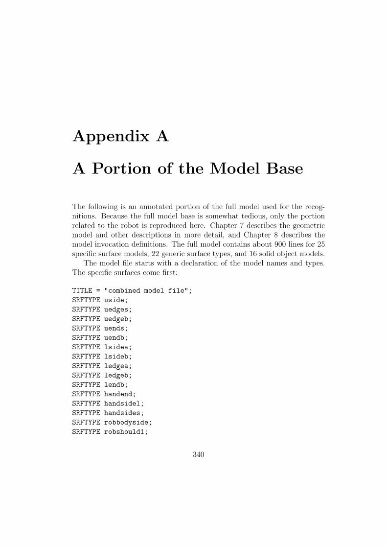
Appendix A

A Portion of the Model Base

The following is an annotated portion of the full model used for the recog-nitions. Because the full model base is somewhat tedious, only the portionrelated to the robot is reproduced here. Chapter 7 describes the geometricmodel and other descriptions in more detail, and Chapter 8 describes themodel invocation definitions. The full model contains about 900 lines for 25specific surface models, 22 generic surface types, and 16 solid object models.

The model file starts with a declaration of the model names and types.The specific surfaces come first:

TITLE = "combined model file";

SRFTYPE uside;

SRFTYPE uedges;

SRFTYPE uedgeb;

SRFTYPE uends;

SRFTYPE uendb;

SRFTYPE lsidea;

SRFTYPE lsideb;

SRFTYPE ledgea;

SRFTYPE ledgeb;

SRFTYPE lendb;

SRFTYPE handend;

SRFTYPE handsidel;

SRFTYPE handsides;

SRFTYPE robbodyside;

SRFTYPE robshould1;

340

A PORTION OF THE MODEL BASE 341

SRFTYPE robshould2;

SRFTYPE robshldend;

SRFTYPE robshoulds;

The declaration of the generic surfaces:

GSRFTYPE quad;

GSRFTYPE trapezium;

GSRFTYPE llgram;

GSRFTYPE rectangle;

GSRFTYPE circle;

GSRFTYPE plane;

GSRFTYPE cylpatch;

GSRFTYPE torus;

GSRFTYPE cylinder;

GSRFTYPE lside;

GSRFTYPE ledge;

GSRFTYPE robshouldg;

GSRFTYPE sapiby2a;

GSRFTYPE sapiby2b;

GSRFTYPE sapiby2c;

GSRFTYPE sapia;

GSRFTYPE sapib;

GSRFTYPE sa3piby2;

GSRFTYPE sapiby2andpi;

The declaration of the solid assemblies:

OBJTYPE hand;

OBJTYPE lowerarm;

OBJTYPE upperarm;

OBJTYPE armasm;

OBJTYPE robshldbd;

OBJTYPE robshldsobj;

OBJTYPE robshould;

OBJTYPE link;

OBJTYPE robbody;

OBJTYPE robot;

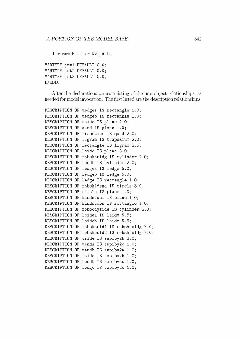
A PORTION OF THE MODEL BASE 342

The variables used for joints:

VARTYPE jnt1 DEFAULT 0.0;

VARTYPE jnt2 DEFAULT 0.0;

VARTYPE jnt3 DEFAULT 0.0;

ENDDEC

After the declarations comes a listing of the interobject relationships, asneeded for model invocation. The first listed are the description relationships:

DESCRIPTION OF uedges IS rectangle 1.0;

DESCRIPTION OF uedgeb IS rectangle 1.0;

DESCRIPTION OF uside IS plane 2.0;

DESCRIPTION OF quad IS plane 1.0;

DESCRIPTION OF trapezium IS quad 2.0;

DESCRIPTION OF llgram IS trapezium 2.0;

DESCRIPTION OF rectangle IS llgram 2.5;

DESCRIPTION OF lside IS plane 3.0;

DESCRIPTION OF robshouldg IS cylinder 2.0;

DESCRIPTION OF lendb IS cylinder 2.0;

DESCRIPTION OF ledgea IS ledge 5.0;

DESCRIPTION OF ledgeb IS ledge 5.0;

DESCRIPTION OF ledge IS rectangle 1.0;

DESCRIPTION OF robshldend IS circle 3.0;

DESCRIPTION OF circle IS plane 1.0;

DESCRIPTION OF handsidel IS plane 1.0;

DESCRIPTION OF handsides IS rectangle 1.0;

DESCRIPTION OF robbodyside IS cylinder 2.0;

DESCRIPTION OF lsidea IS lside 5.5;

DESCRIPTION OF lsideb IS lside 5.5;

DESCRIPTION OF robshould1 IS robshouldg 7.0;

DESCRIPTION OF robshould2 IS robshouldg 7.0;

DESCRIPTION OF uside IS sapiby2b 2.0;

DESCRIPTION OF uends IS sapiby2c 1.0;

DESCRIPTION OF uendb IS sapiby2a 1.0;

DESCRIPTION OF lside IS sapiby2b 1.0;

DESCRIPTION OF lendb IS sapiby2c 1.0;

DESCRIPTION OF ledge IS sapiby2c 1.0;

A PORTION OF THE MODEL BASE 343

DESCRIPTION OF handsides IS sapiby2andpi 1.0;

DESCRIPTION OF handsidel IS sapiby2andpi 1.0;

DESCRIPTION OF handend IS sapiby2andpi 1.0;

DESCRIPTION OF robshldend IS sapiby2b 1.0;

DESCRIPTION OF robshouldg IS sapiby2a 0.5;

DESCRIPTION OF robshoulds IS sapib 0.5;

DESCRIPTION OF cylinder IS cylpatch 2.0;

DESCRIPTION OF uendb IS cylinder 2.0;

DESCRIPTION OF uends IS cylinder 2.0;

The subcomponent relationships:

SUBCOMPONENT OF hand IS handend 0.90;

SUBCOMPONENT OF hand IS handsidel 0.90;

SUBCOMPONENT OF hand IS handsides 0.90;

SUBCOMPONENT OF link IS robshould 1.00;

SUBCOMPONENT OF link IS armasm 1.00;

SUBCOMPONENT OF lowerarm IS hand 0.90;

SUBCOMPONENT OF lowerarm IS ledgea 0.90;

SUBCOMPONENT OF lowerarm IS ledgeb 0.90;

SUBCOMPONENT OF lowerarm IS lendb 0.90;

SUBCOMPONENT OF lowerarm IS lsidea 0.90;

SUBCOMPONENT OF lowerarm IS lsideb 0.90;

SUBCOMPONENT OF robbody IS robbodyside 0.90;

SUBCOMPONENT OF robot IS link 1.00;

SUBCOMPONENT OF robot IS robbody 1.00;

SUBCOMPONENT OF robshldbd IS robshldend 0.90;

SUBCOMPONENT OF robshldbd IS robshould1 0.90;

SUBCOMPONENT OF robshldbd IS robshould2 0.90;

SUBCOMPONENT OF robshldsobj IS robshoulds 0.90;

SUBCOMPONENT OF robshould IS robshldbd 0.90;

SUBCOMPONENT OF robshould IS robshldsobj 0.90;

SUBCOMPONENT OF upperarm IS uedgeb 0.90;

SUBCOMPONENT OF upperarm IS uedges 0.90;

SUBCOMPONENT OF upperarm IS uendb 0.90;

SUBCOMPONENT OF upperarm IS uends 0.90;

SUBCOMPONENT OF upperarm IS uside 0.90;

SUBCOMPONENT OF armasm IS lowerarm 0.80;

SUBCOMPONENT OF armasm IS upperarm 0.80;

A PORTION OF THE MODEL BASE 344

The supercomponent relationships:

SUPERCOMPONENT OF hand IS lowerarm 0.10;

SUPERCOMPONENT OF handend IS hand 0.10;

SUPERCOMPONENT OF handsidel IS hand 0.10;

SUPERCOMPONENT OF handsides IS hand 0.10;

SUPERCOMPONENT OF ledgea IS lowerarm 0.10;

SUPERCOMPONENT OF ledgeb IS lowerarm 0.10;

SUPERCOMPONENT OF lendb IS lowerarm 0.10;

SUPERCOMPONENT OF link IS robot 0.10;

SUPERCOMPONENT OF lowerarm IS armasm 0.10;

SUPERCOMPONENT OF lsidea IS lowerarm 0.10;

SUPERCOMPONENT OF lsideb IS lowerarm 0.10;

SUPERCOMPONENT OF robbody IS robot 0.10;

SUPERCOMPONENT OF robbodyside IS robbody 0.10;

SUPERCOMPONENT OF robshldbd IS robshould 0.10;

SUPERCOMPONENT OF robshldend IS robshldbd 0.10;

SUPERCOMPONENT OF robshldsobj IS robshould 0.10;

SUPERCOMPONENT OF robshould IS link 0.10;

SUPERCOMPONENT OF robshould1 IS robshldbd 0.10;

SUPERCOMPONENT OF robshould2 IS robshldbd 0.10;

SUPERCOMPONENT OF robshoulds IS robshldsobj 0.10;

SUPERCOMPONENT OF uedgeb IS upperarm 0.10;

SUPERCOMPONENT OF uedges IS upperarm 0.10;

SUPERCOMPONENT OF uendb IS upperarm 0.10;

SUPERCOMPONENT OF uends IS upperarm 0.10;

SUPERCOMPONENT OF upperarm IS armasm 0.10;

SUPERCOMPONENT OF armasm IS link 0.10;

SUPERCOMPONENT OF uside IS upperarm 0.10;

The general association relationships:

ASSOCIATION OF upperarm IS lowerarm 1.0;

ASSOCIATION OF lowerarm IS upperarm 1.0;

The competitor relationships amongst generic types:

COMPETITOR OF plane IS cylpatch 1.0;

COMPETITOR OF cylpatch IS plane 1.0;

A PORTION OF THE MODEL BASE 345

COMPETITOR OF torus IS plane 1.0;

COMPETITOR OF plane IS torus 1.0;

COMPETITOR OF cylpatch IS torus 1.0;

COMPETITOR OF torus IS cylpatch 1.0;

COMPETITOR OF lside IS ledge 1.0;

COMPETITOR OF lside IS robshouldg 1.0;

COMPETITOR OF ledge IS lside 1.0;

COMPETITOR OF ledge IS robshouldg 1.0;

COMPETITOR OF robshouldg IS lside 1.0;

COMPETITOR OF robshouldg IS ledge 1.0;

ENDNET

After the relationships comes the listing of the visibility groups and whatfeatures are seen in each. This information is used to help create the invo-cation network.

SUBCGRP OF robot = robbody link;

SUBCGRP OF link = robshould armasm;

SUBCGRP OF armasm = upperarm lowerarm;

SUBCGRP OF upperarm = uside uends uedgeb uedges;

SUBCGRP OF upperarm = uside uendb uedgeb uedges;

SUBCGRP OF lowerarm = lendb lsidea ledgea;

SUBCGRP OF lowerarm = lendb lsideb ledgea;

SUBCGRP OF lowerarm = lendb lsideb ledgeb;

SUBCGRP OF lowerarm = lendb lsidea ledgeb;

SUBCGRP OF hand = handend handsides handsidel;

SUBCGRP OF robbody = robbodyside;

SUBCGRP OF robshould = robshldbd robshldsobj;

SUBCGRP OF robshldbd = robshould1 robshldend;

SUBCGRP OF robshldbd = robshould2 robshldend;

SUBCGRP OF robshldsobj = robshoulds;

ENDGRP

The next section lists the unary property evidence constraints, whichare used for property evaluations during model invocation. Binary evidenceconstraints were not explicit in IMAGINE I. There may not always bemany properties listed for an object, because (1) it may be a generic object,(2) the other properties are represented in a description or (3) the propertyis irrelevant.

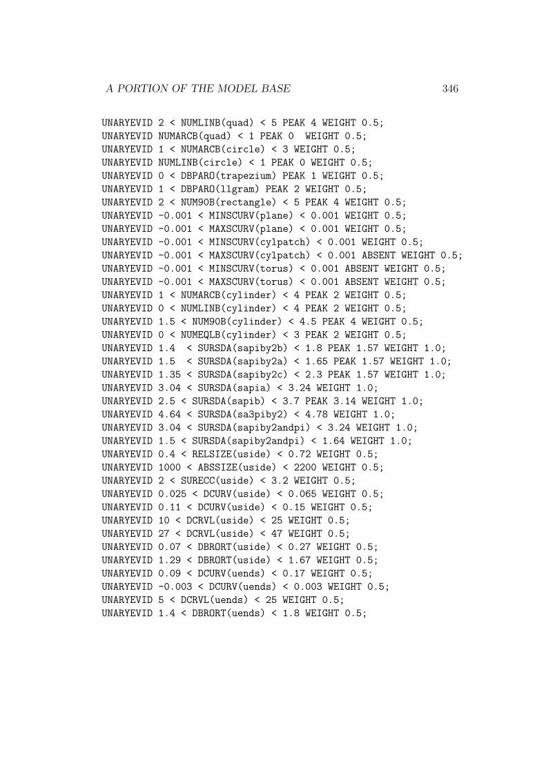
A PORTION OF THE MODEL BASE 346

UNARYEVID 2 < NUMLINB(quad) < 5 PEAK 4 WEIGHT 0.5;

UNARYEVID NUMARCB(quad) < 1 PEAK 0 WEIGHT 0.5;

UNARYEVID 1 < NUMARCB(circle) < 3 WEIGHT 0.5;

UNARYEVID NUMLINB(circle) < 1 PEAK 0 WEIGHT 0.5;

UNARYEVID 0 < DBPARO(trapezium) PEAK 1 WEIGHT 0.5;

UNARYEVID 1 < DBPARO(llgram) PEAK 2 WEIGHT 0.5;

UNARYEVID 2 < NUM90B(rectangle) < 5 PEAK 4 WEIGHT 0.5;

UNARYEVID -0.001 < MINSCURV(plane) < 0.001 WEIGHT 0.5;

UNARYEVID -0.001 < MAXSCURV(plane) < 0.001 WEIGHT 0.5;

UNARYEVID -0.001 < MINSCURV(cylpatch) < 0.001 WEIGHT 0.5;

UNARYEVID -0.001 < MAXSCURV(cylpatch) < 0.001 ABSENT WEIGHT 0.5;

UNARYEVID -0.001 < MINSCURV(torus) < 0.001 ABSENT WEIGHT 0.5;

UNARYEVID -0.001 < MAXSCURV(torus) < 0.001 ABSENT WEIGHT 0.5;

UNARYEVID 1 < NUMARCB(cylinder) < 4 PEAK 2 WEIGHT 0.5;

UNARYEVID 0 < NUMLINB(cylinder) < 4 PEAK 2 WEIGHT 0.5;

UNARYEVID 1.5 < NUM90B(cylinder) < 4.5 PEAK 4 WEIGHT 0.5;

UNARYEVID 0 < NUMEQLB(cylinder) < 3 PEAK 2 WEIGHT 0.5;

UNARYEVID 1.4 < SURSDA(sapiby2b) < 1.8 PEAK 1.57 WEIGHT 1.0;

UNARYEVID 1.5 < SURSDA(sapiby2a) < 1.65 PEAK 1.57 WEIGHT 1.0;

UNARYEVID 1.35 < SURSDA(sapiby2c) < 2.3 PEAK 1.57 WEIGHT 1.0;

UNARYEVID 3.04 < SURSDA(sapia) < 3.24 WEIGHT 1.0;

UNARYEVID 2.5 < SURSDA(sapib) < 3.7 PEAK 3.14 WEIGHT 1.0;

UNARYEVID 4.64 < SURSDA(sa3piby2) < 4.78 WEIGHT 1.0;

UNARYEVID 3.04 < SURSDA(sapiby2andpi) < 3.24 WEIGHT 1.0;

UNARYEVID 1.5 < SURSDA(sapiby2andpi) < 1.64 WEIGHT 1.0;

UNARYEVID 0.4 < RELSIZE(uside) < 0.72 WEIGHT 0.5;

UNARYEVID 1000 < ABSSIZE(uside) < 2200 WEIGHT 0.5;

UNARYEVID 2 < SURECC(uside) < 3.2 WEIGHT 0.5;

UNARYEVID 0.025 < DCURV(uside) < 0.065 WEIGHT 0.5;

UNARYEVID 0.11 < DCURV(uside) < 0.15 WEIGHT 0.5;

UNARYEVID 10 < DCRVL(uside) < 25 WEIGHT 0.5;

UNARYEVID 27 < DCRVL(uside) < 47 WEIGHT 0.5;

UNARYEVID 0.07 < DBRORT(uside) < 0.27 WEIGHT 0.5;

UNARYEVID 1.29 < DBRORT(uside) < 1.67 WEIGHT 0.5;

UNARYEVID 0.09 < DCURV(uends) < 0.17 WEIGHT 0.5;

UNARYEVID -0.003 < DCURV(uends) < 0.003 WEIGHT 0.5;

UNARYEVID 5 < DCRVL(uends) < 25 WEIGHT 0.5;

UNARYEVID 1.4 < DBRORT(uends) < 1.8 WEIGHT 0.5;

A PORTION OF THE MODEL BASE 347

UNARYEVID 1.8 < SURECC(uends) < 2.6 WEIGHT 0.5;

UNARYEVID 130 < ABSSIZE(uends) < 250 WEIGHT 0.5;

UNARYEVID 0.04 < RELSIZE(uends) < 0.11 WEIGHT 0.5;

UNARYEVID 0.11 < MAXSCURV(uends) < 0.15 WEIGHT 0.5;

UNARYEVID 0.08 < RELSIZE(uendb) < 0.16 WEIGHT 0.5;

UNARYEVID 210 < ABSSIZE(uendb) < 430 WEIGHT 0.5;

UNARYEVID 2.8 < SURECC(uendb) < 4 WEIGHT 0.5;

UNARYEVID 1.47 < DBRORT(uendb) < 1.67 WEIGHT 0.5;

UNARYEVID 5 < DCRVL(uendb) < 15 WEIGHT 0.5;

UNARYEVID 27 < DCRVL(uendb) < 37 WEIGHT 0.5;

UNARYEVID 0.025 < DCURV(uendb) < 0.065 WEIGHT 0.5;

UNARYEVID 2.8 < SURSDA(uedges) < 3.4 WEIGHT 1.0;

UNARYEVID 1.4 < SURSDA(uedges) < 1.8 WEIGHT 0.5;

UNARYEVID 5 < DCRVL(uedges) < 25 WEIGHT 0.5;

UNARYEVID 1.47 < DBRORT(uedges) < 1.67 WEIGHT 0.5;

UNARYEVID 0.04 < RELSIZE(uedges) < 0.15 WEIGHT 0.5;

UNARYEVID 140 < ABSSIZE(uedges) < 260 WEIGHT 0.5;

UNARYEVID 1.8 < SURECC(uedges) < 2.6 WEIGHT 0.5;

UNARYEVID 2.9 < SURSDA(uedgeb) < 3.1 WEIGHT 1.0;

UNARYEVID 1.45 < SURSDA(uedgeb) < 1.85 WEIGHT 1.0;

UNARYEVID 0.11 < RELSIZE(uedgeb) < 0.22 WEIGHT 0.5;

UNARYEVID 290 < ABSSIZE(uedgeb) < 570 WEIGHT 0.5;

UNARYEVID 3.6 < SURECC(uedgeb) < 5.2 WEIGHT 0.5;

UNARYEVID 1.47 < DBRORT(uedgeb) < 1.67 WEIGHT 0.5;

UNARYEVID 5 < DCRVL(uedgeb) < 15 WEIGHT 0.5;

UNARYEVID 38 < DCRVL(uedgeb) < 48 WEIGHT 0.5;

UNARYEVID 0.51 < RELSIZE(lside) < 0.65 WEIGHT 0.5;

UNARYEVID 460 < ABSSIZE(lside) < 910 WEIGHT 0.5;

UNARYEVID 2.3 < SURECC(lside) < 3.3 WEIGHT 0.5;

UNARYEVID 1.07 < DBRORT(lside) < 1.47 WEIGHT 0.5;

UNARYEVID 1.37 < DBRORT(lside) < 1.77 WEIGHT 0.5;

UNARYEVID 3.6 < DCRVL(lside) < 24 WEIGHT 0.5;

UNARYEVID 32.8 < DCRVL(lside) < 54 WEIGHT 0.5;

UNARYEVID 0.06 < DCURV(lside) < 0.12 WEIGHT 0.5;

UNARYEVID 1.8 < SURECC(lendb) < 2.9 WEIGHT 0.5;

UNARYEVID 70 < ABSSIZE(lendb) < 200 WEIGHT 0.5;

UNARYEVID 0.07 < RELSIZE(lendb) < 0.18 WEIGHT 0.5;

UNARYEVID 0.97 < DBRORT(lendb) < 2.17 WEIGHT 0.5;

A PORTION OF THE MODEL BASE 348

UNARYEVID 4 < DCRVL(lendb) < 13 WEIGHT 0.5;

UNARYEVID 13 < DCRVL(lendb) < 27 WEIGHT 0.5;

UNARYEVID 0.07 < DCURV(lendb) < 0.14 WEIGHT 0.5;

UNARYEVID 33 < DCRVL(ledgea) < 55 WEIGHT 0.5;

UNARYEVID 3.6 < DCRVL(ledgea) < 13.6 WEIGHT 0.5;

UNARYEVID 3.6 < DCRVL(ledgeb) < 13.6 WEIGHT 0.5;

UNARYEVID 32 < DCRVL(ledgeb) < 54 WEIGHT 0.5;

UNARYEVID 0.26 < RELSIZE(ledge) < 0.38 WEIGHT 0.5;

UNARYEVID 230 < ABSSIZE(ledge) < 470 WEIGHT 0.5;

UNARYEVID 4.6 < SURECC(ledge) < 6.6 WEIGHT 0.5;

UNARYEVID 1.4 < DBRORT(ledge) < 1.8 WEIGHT 0.5;

UNARYEVID 0.20 < RELSIZE(handsides) < 0.28 WEIGHT 0.5;

UNARYEVID 56 < ABSSIZE(handsides) < 76 WEIGHT 0.5;

UNARYEVID 1 < SURECC(handsides) < 1.3 WEIGHT 0.5;

UNARYEVID 1.47 < DBRORT(handsides) < 1.67 WEIGHT 0.5;

UNARYEVID 2.7 < DCRVL(handsides) < 13.6 WEIGHT 0.5;

UNARYEVID 0.30 < RELSIZE(handsidel) < 0.38 WEIGHT 0.5;

UNARYEVID 80 < ABSSIZE(handsidel) < 110 WEIGHT 0.5;

UNARYEVID 1.2 < SURECC(handsidel) < 1.6 WEIGHT 0.5;

UNARYEVID 1.47 < DBRORT(handsidel) < 1.67 WEIGHT 0.5;

UNARYEVID 1 < DBPARO(handsidel) < 3 WEIGHT 0.3;

UNARYEVID 2.7 < DCRVL(handsidel) < 18.5 WEIGHT 0.5;

UNARYEVID 0.21 < DCURV(handsidel) < 0.25 WEIGHT 0.5;

UNARYEVID 0.21 < MAXSCURV(handend) < 0.25 WEIGHT 0.5;

UNARYEVID 0.32 < RELSIZE(handend) < 0.52 WEIGHT 0.5;

UNARYEVID 96 < ABSSIZE(handend) < 136 WEIGHT 0.5;

UNARYEVID 1 < SURECC(handend) < 1.2 WEIGHT 0.5;

UNARYEVID 1.47 < DBRORT(handend) < 1.67 WEIGHT 0.5;

UNARYEVID 3.6 < DCRVL(handend) < 18.5 WEIGHT 0.5;

UNARYEVID 0.21 < DCURV(handend) < 0.25 WEIGHT 0.5;

UNARYEVID 4.5 < SURSDA(robbodyside) < 4.9 WEIGHT 0.5;

UNARYEVID 2.5 < SURSDA(robbodyside) < 3.7 WEIGHT 0.5;

UNARYEVID 0.09 < MAXSCURV(robbodyside) < 0.14 WEIGHT 0.5;

UNARYEVID 0.9 < RELSIZE(robbodyside) < 1.1 WEIGHT 0.5;

UNARYEVID 1200 < ABSSIZE(robbodyside) < 1600 WEIGHT 0.5;

UNARYEVID 1.57 < SURECC(robbodyside) < 3.5 WEIGHT 0.5;

UNARYEVID 1.17 < DBRORT(robbodyside) < 1.97 WEIGHT 0.5;

UNARYEVID 1 < DBPARO(robbodyside) < 3 WEIGHT 0.3;

A PORTION OF THE MODEL BASE 349

UNARYEVID 20 < DCRVL(robbodyside) < 36 WEIGHT 0.5;

UNARYEVID 40 < DCRVL(robbodyside) < 60 WEIGHT 0.5;

UNARYEVID -0.003 < DCURV(robbodyside) < 0.015 WEIGHT 0.5;

UNARYEVID 0.05 < DCURV(robbodyside) < 0.16 WEIGHT 0.5;

UNARYEVID 0.11 < RELSIZE(robshldend) < 0.40 WEIGHT 0.5;

UNARYEVID 156 < ABSSIZE(robshldend) < 248 WEIGHT 0.5;

UNARYEVID 0.9 < SURECC(robshldend) < 1.5 WEIGHT 0.5;

UNARYEVID 3.04 < DBRORT(robshldend) < 3.24 WEIGHT 0.5;

UNARYEVID 0 < DBPARO(robshldend) < 2 WEIGHT 0.3;

UNARYEVID 20.1 < DCRVL(robshldend) < 40 WEIGHT 0.5;

UNARYEVID 0.08 < DCURV(robshldend) < 0.15 WEIGHT 0.5;

UNARYEVID 0.105 < MAXSCURV(robshouldg) < 0.145 WEIGHT 0.5;

UNARYEVID -0.003 < MINSCURV(robshouldg) < 0.01 WEIGHT 0.5;

UNARYEVID 0.55 < RELSIZE(robshouldg) < 0.79 WEIGHT 0.5;

UNARYEVID 428 < ABSSIZE(robshouldg) < 828 WEIGHT 0.5;

UNARYEVID 1.5 < SURECC(robshouldg) < 3.5 WEIGHT 0.5;

UNARYEVID 1.4 < DBRORT(robshouldg) < 1.8 WEIGHT 0.5;

UNARYEVID 0.8 < DBRORT(robshouldg) < 1.1 WEIGHT 0.5;

UNARYEVID 0.9 < DBRORT(robshouldg) < 1.5 WEIGHT 0.5;

UNARYEVID 1 < DBPARO(robshouldg) < 3 WEIGHT 0.3;

UNARYEVID 5 < DCRVL(robshouldg) < 16 WEIGHT 0.5;

UNARYEVID 11 < DCRVL(robshouldg) < 21 WEIGHT 0.5;

UNARYEVID 18 < DCRVL(robshouldg) < 37 WEIGHT 0.5;

UNARYEVID 0.071 < DCURV(robshouldg) < 0.15 WEIGHT 0.5;

UNARYEVID -0.003 < DCURV(robshouldg) < 0.035 WEIGHT 0.5;

UNARYEVID 0.105 < MAXSCURV(robshoulds) < 0.145 WEIGHT 0.5;

UNARYEVID -0.003 < MINSCURV(robshoulds) < 0.01 WEIGHT 0.5;

UNARYEVID 0.9 < RELSIZE(robshoulds) < 1.1 WEIGHT 0.5;

UNARYEVID 60 < ABSSIZE(robshoulds) < 140 WEIGHT 0.5;

UNARYEVID 2 < SURECC(robshoulds) < 4 WEIGHT 0.5;

UNARYEVID 1.8 < DBRORT(robshoulds) < 2.6 WEIGHT 0.5;

UNARYEVID 1.5 < DBRORT(robshoulds) < 2.3 WEIGHT 0.5;

UNARYEVID -1 < DBPARO(robshoulds) < 1 WEIGHT 0.3;

UNARYEVID 6 < DCRVL(robshoulds) < 18 WEIGHT 0.5;

UNARYEVID 18 < DCRVL(robshoulds) < 30 WEIGHT 0.5;

UNARYEVID 0.03 < DCURV(robshoulds) < 0.131 WEIGHT 0.5;

ENDINV

A PORTION OF THE MODEL BASE 350

The next section gives the geometric model for the specific surfaces. Thesyntax of the models is described in Chapter 7. The DEFAULT values are aposition that can be used for drawing the models.

SURFACE uside DEFAULT ((0,0,1000),(0,0,0)) =

PO/(0,0,0) BO/LINE

PO/(19.6,0,0) BO/LINE

PC/(61.8,7.4,0) BO/CURVE[7.65,0,0]

PC/(61.8,22.4,0) BO/LINE

PO/(19.6,29.8,0) BO/LINE

PO/(0,29.8,0) BO/CURVE[-22.42,0,0]

PLANE

NORMAL AT (10,15,0) = (0,0,-1);

SURFACE uedges DEFAULT ((0,0,1000),(0,0,0)) =

PO/(0,0,0) BO/LINE

PO/(19.6,0,0) BO/LINE

PO/(19.6,10,0) BO/LINE

PO/(0,10,0) BO/LINE

PLANE

NORMAL AT (10,5,0) = (0,0,-1);

SURFACE uedgeb DEFAULT ((0,0,1000),(0,0,0)) =

PO/(0,0,0) BO/LINE

PO/(42.85,0,0) BO/LINE

PO/(42.85,10,0) BCW/LINE

PO/(0,10,0) BO/LINE

PLANE

NORMAL AT (21,5,0) = (0,0,-1);

SURFACE uends DEFAULT ((0,0,1000),(0,0,0)) =

PO/(0,0,0) BCW/LINE

PO/(10,0,0) BO/CURVE[0,0,-7.65]

PO/(10,15,0) BCW/LINE

PO/(0,15,0) BO/CURVE[0,0,-7.65]

CYLINDER[(0,7.5,1.51),(10,7.5,1.51),7.65,7.65]

NORMAL AT (5,7.5,-6.14) = (0,0,-1);

SURFACE uendb DEFAULT ((0,0,1000),(0,0,0)) =

PO/(0,0,0) BO/LINE

PO/(10,0,0) BO/CURVE[0,0,-22.42]

PO/(10,29.8,0) BO/LINE

A PORTION OF THE MODEL BASE 351

PO/(0,29.8,0) BO/CURVE[0,0,-22.42]

CYLINDER [(0,14.9,16.75),(10,14.9,16.75),22.42,22.42]

NORMAL AT (5,15,-5.67) = (0,0,-1);

SURFACE lsidea DEFAULT ((0,0,1000),(0,0,0)) =

PO/(0,0,0) BO/LINE

PO/(44,0,0) BN/LINE

PO/ (44,8.6,0) BN/LINE

PO/(2,17,0) BN/CURVE[-10.96,1.29,0]

PLANE

NORMAL AT (22,6,0) = (0,0,-1);

SURFACE lsideb DEFAULT ((0,0,1000),(0,0,0)) =

PO/(0,0,0) BO/LINE

PO/(-44,0,0) BN/LINE

PO/(-44,8.6,0) BO/LINE

PO/(-2,17,0) BO/CURVE[10.96,1.29,0]

PLANE

NORMAL AT (-22,6,0) = (0,0,-1);

SURFACE ledgea DEFAULT ((0,0,1000),(0,0,0)) =

PO/(0,0,0) BO/LINE

PO/(44,0,0) BN/LINE

PO/(44,8.6,0) BO/LINE

PO/(0,8.6,0) BO/LINE

PLANE

NORMAL AT (22,4.3,0) = (0,0,-1);

SURFACE ledgeb DEFAULT ((0,0,1000),(0,0,0)) =

PO/(0,0,0) BO/LINE

PO/(42.8,0,0) BN/LINE

PO/ (42.8,8.6,0) BO/LINE

PO/ (0,8.6,0) BO/LINE

PLANE

NORMAL AT (22,4.3,0) = (0,0,-1);

SURFACE lendb DEFAULT ((0,0,1000),(0,0,0)) =

PO/(0,0,0) BO/CURVE[0,0,-11.04]

PO/(17,0,0) BO/LINE

PO/(17,8.6,0) BO/CURVE[0,0,-11.04]

PO/(0,8.6,0) BO/LINE

CYLINDER [(8.5,0,7.04),(8.5,8.6,7.04),11.04,11.04]

NORMAL AT (8.5,4.3,-4) = (0,0,-1);

A PORTION OF THE MODEL BASE 352

SURFACE handsides DEFAULT ((0,0,1000),(0,0,0)) =

PO/(0,0,0) BO/LINE

PO/(7.7,0,0) BCW/LINE

PO/(7.7,8.6,0) BO/LINE

PO/(0,8.6,0) BO/LINE

PLANE

NORMAL AT (3.8,4.3,0) = (0,0,-1);

SURFACE handsidel DEFAULT ((0,0,1000),(0,0,0)) =

PO/(0,0,0) BO/LINE

PO/(0,8.6,0) BO/LINE

PO/(7.7,8.6,0) BO/CURVE[3.04,3.04,0]

PN/(12,4.3,0) BO/CURVE[3.04,-3.04,0]

PO/(7.7,0,0) BO/LINE

PLANE

NORMAL AT (6,4.3,0) = (0,0,-1);

SURFACE handend DEFAULT ((0,0,1000),(0,0,0)) =

PO/(0,0,0) BO/CURVE[0,-3.04,-3.04]

PN/(0,4.3,-4.3) BO/CURVE[0,3.04,-3.04]

PO/(0,8.6,0) BCW/LINE

PO/(8.6,8.6,0) BO/CURVE[0,3.04,-3.04]

PN/(8.6,4.3,-4.3) BO/CURVE[0,-3.04,-3.04]

PO/(8.6,0,0) BCW/LINE

CYLINDER [(0,4.3,0),(8.6,4.3,0),4.3,4.3]

NORMAL AT (4.3,4.3,-4.3) = (0,0,-1);

SURFACE robbodyside DEFAULT ((0,0,1000),(0,0,0)) =

PO/(-9,0,0) BO/CURVE[-6.364,0,-6.364]

PN/(0,0,-9) BO/CURVE[6.364,0,-6.364]

PO/(9,0,0) BN/LINE

PO/(9,50,0) BO/CURVE[6.364,0,-6.364]

PN/(0,50,-9) BO/CURVE[-6.364,0,-6.364]

PO/(-9,50,0) BN/LINE

CYLINDER [(0,0,0),(0,50,0),9,9]

NORMAL AT (0,25,-9) = (0,0,-1);

SURFACE robshldend DEFAULT ((0,0,1000),(0,0,0)) =

PN/(-8,0,0) BO/CURVE[-5.66,5.66,0]

PN/(0,8,0) BO/CURVE[5.66,5.66,0]

PN/(8,0,0) BO/CURVE[5.66,-5.66,0]

PN/(0,-8,0) BO/CURVE[-5.66,-5.66,0]

A PORTION OF THE MODEL BASE 353

PLANE

NORMAL AT (0,0,0) = (0,0,-1);

SURFACE robshoulds DEFAULT ((0,0,1000),(0,0,0)) =

PO/(-8,0,0) BO/CURVE[-5.66,0,-5.66]

PN/(0,0,-8) BO/CURVE[5.66,0,-5.66]

PO/(8,0,0) BO/CURVE[0,-6.32,-6.32]

PO/(0,8,-8) BO/CURVE[0,-6.32,-6.32]

CYLINDER [(0,0,0),(0,1,0),8,8]

NORMAL AT (0,4,-8) = (0,0,-1);

SURFACE robshould1 DEFAULT ((0,0,1000),(0,0,0)) =

PO/(0,-8,0) BO/CURVE[0,-5.66,-5.66]

PN/(0,0,-8) BO/CURVE[0,5.66,-5.66]

PO/(0,8,0) BN/LINE

PO/(29,8,0) BO/CURVE[0,5.66,-5.66]

PN/(29,0,-8) BO/CURVE[0,-5.66,-5.66]

PO/(29,-8,0) BN/LINE

PO/(27,-8,0) BO/CURVE[0,-6.32,-6.32]

PO/(19,0,-8) BO/CURVE[0,-6.32,-6.32]

PO/(11,-8,0) BN/LINE

CYLINDER [(0,0,0),(1,0,0),8,8]

NORMAL AT (10,0,-8) = (0,0,-1);

SURFACE robshould2 DEFAULT ((0,0,1000),(0,0,0)) =

PO/(0,-8,0) BO/CURVE[0,-5.66,-5.66]

PN/(0,0,-8) BO/CURVE[0,5.66,-5.66]

PO/(0,8,0) BN/LINE

PO/(-29,8,0) BO/CURVE[0,5.66,-5.66]

PN/(-29,0,-8) BO/CURVE[0,-5.66,-5.66]

PO/(-29,-8,0) BN/LINE

PO/(-27,-8,0) BO/CURVE[0,-6.32,-6.32]

PO/(-19,0,-8) BO/CURVE[0,-6.32,-6.32]

PO/(-11,-8,0) BN/LINE

CYLINDER [(0,0,0),(-1,0,0),8,8]

NORMAL AT (-10,0,-8) = (0,0,-1);

Then come the geometric models for the ASSEMBLYs:

ASSEMBLY robot DEFAULT ((0,0,1000),(0,0.7,4)) =

robbody AT ((0,0,0),(0,0,0))

A PORTION OF THE MODEL BASE 354

link AT ((0,50,0),(0,0,0))

FLEX ((0,0,0),(0,jnt1,3.14159));

ASSEMBLY link DEFAULT ((0,0,1000),(0,0.7,4)) =

robshould AT ((0,0,0),(0,0,0))

armasm AT ((0,8,-19),(0,0,0))

FLEX ((0,0,0),(jnt2,0,0));

ASSEMBLY armasm DEFAULT ((0,0,1000),(0,0.7,4)) =

upperarm AT ((0,0,0),(0,0,0))

lowerarm AT ((43.5,0,0),(0,0,0))

FLEX ((0,0,0),(jnt3,0,0));

ASSEMBLY upperarm DEFAULT ((0,0,1000),(0,0.7,4)) =

uside AT ((-17,-14.9,-10),(0,0,0))

uside AT ((-17,14.9,0),(0,3.14,1.5707))

uendb AT ((-17,-14.9,0),(0,1.5707,3.14159))

uends AT ((44.8,-7.5,-10),(0,1.5707,0))

uedges AT ((-17,-14.9,0),(0,1.5707,4.7123))

uedges AT ((-17,14.9,-10),(0,1.5707,1.5707))

uedgeb AT ((2.6,-14.9,0),(0.173,1.5707,4.7123))

uedgeb AT ((2.6,14.9,-10),(6.11,1.5707,1.5707));

ASSEMBLY lowerarm DEFAULT ((0,0,1000),(0,0.7,4)) =

lsidea AT ((-9.4,-7.7,0),(0,0,0))

lsideb AT ((-9.4,-7.7,8.6),(0,3.14,0))

lendb AT ((-9.4,-7.7,0),(1.4536,1.5707,1.5707))

ledgea AT ((-9.4,-7.7,8.6),(0,1.5707,4.7123))

ledgeb AT ((-7.4,9.3,0),(6.083,1.5707,1.5707))

hand AT ((34.6,-3.8,4.3),(0,0,0));

ASSEMBLY hand DEFAULT ((0,0,1000),(0,0.7,4)) =

handsidel AT ((0,-4.3,-4.3),(0,0,0))

handsidel AT ((0,4.3,4.3),(0,3.14,1.5707))

handsides AT ((0,-4.3,4.3),(0,1.5707,4.71))

handsides AT ((0,4.3,-4.3),(0,1.5707,1.5707))

handend AT ((7.7,-4.3,-4.3),(0,1.57,0));

ASSEMBLY robbody DEFAULT ((0,0,1000),(0,0.7,4)) =

robbodyside AT ((0,0,0),(0,0,0))

robbodyside AT ((0,0,0),(0,3.14,0));

ASSEMBLY robshould DEFAULT ((0,0,1000),(0,0.7,4)) =

robshldbd AT ((0,0,0),(0,0,0))

robshldsobj AT ((0,0,0),(0,0,0));

A PORTION OF THE MODEL BASE 355

ASSEMBLY robshldbd DEFAULT ((0,0,1000),(0,0.7,4)) =

robshould1 AT ((0,8,-19),(0,1.5707,0))

robshould2 AT ((0,8,-19),(0,1.5707,3.14159))

robshldend AT ((0,8,10),(0,3.14,0));

ASSEMBLY robshldsobj DEFAULT ((0,0,1000),(0,0.7,4)) =

robshoulds AT ((0,0,0),(0,1.5707,0))

robshoulds AT ((0,0,0),(0,1.5707,3.14159));

ENDSTR

Lastly, there are the additional property constraints used by verification:

CONSTRAINT uside MAXSCURV(uside) < 0.05

CONSTRAINT uside ABSSIZE(uside) < 1900.0

CONSTRAINT uside ABSSIZE(uside) > 1050.0

CONSTRAINT uends ABSSIZE(uends) < 250.0

CONSTRAINT uendb ABSSIZE(uendb) < 430.0

CONSTRAINT uedges ABSSIZE(uedges) < 260.0

CONSTRAINT uedges SURECC(uedges) < 3.0

CONSTRAINT uedgeb ABSSIZE(uedgeb) < 570.0

CONSTRAINT lsidea ABSSIZE(lsidea) < 910.0

CONSTRAINT lsidea ABSSIZE(lsidea) > 300.0

CONSTRAINT lsideb ABSSIZE(lsideb) < 910.0

CONSTRAINT lsideb ABSSIZE(lsideb) > 300.0

CONSTRAINT lendb ABSSIZE(lendb) < 200.0

CONSTRAINT ledgea ABSSIZE(ledgea) < 470.0

CONSTRAINT ledgea ABSSIZE(ledgea) > 200.0

CONSTRAINT ledgeb ABSSIZE(ledgeb) < 470.0

CONSTRAINT ledgeb ABSSIZE(ledgeb) > 200.0

CONSTRAINT handsides ABSSIZE(handsides) < 76.0

CONSTRAINT handsidel ABSSIZE(handsidel) < 110.0

CONSTRAINT handend ABSSIZE(handend) < 136.0

CONSTRAINT robbodyside ABSSIZE(robbodyside) < 1600.0

CONSTRAINT robshldend ABSSIZE(robshldend) < 248.0

CONSTRAINT robshldend SURECC(robshldend) < 1.5

CONSTRAINT robshould1 ABSSIZE(robshould1) < 828.0

CONSTRAINT robshould2 ABSSIZE(robshould2) < 828.0

CONSTRAINT robshoulds ABSSIZE(robshoulds) < 130.0

CONSTRAINT robbodyside SURECC(robbodyside) > 2.0

A PORTION OF THE MODEL BASE 356

CONSTRAINT robbodyside MAXSCURV(robbodyside) > 0.095

ENDCON

STOP