from steiner formulas for cones to concentration of...

FROM STEINER FORMULAS FOR CONESTO CONCENTRATION OF INTRINSIC VOLUMES

MICHAEL B. MCCOY AND JOEL A. TROPP

ABSTRACT. The intrinsic volumes of a convex cone are geometric functionals that return basic structural informationabout the cone. Recent research has demonstrated that conic intrinsic volumes are valuable for understanding thebehavior of random convex optimization problems. This paper develops a systematic technique for studying conicintrinsic volumes using methods from probability. At the heart of this approach is a general Steiner formula forcones. This result converts questions about the intrinsic volumes into questions about the projection of a Gaussianrandom vector onto the cone, which can then be resolved using tools from Gaussian analysis. The approach leads tonew identities and bounds for the intrinsic volumes of a cone, including a near-optimal concentration inequality.

1. INTRODUCTION

In the 1840s, Steiner developed a striking decomposition for the volume of a Euclidean expansion of apolytope in R3. The modern statement of Steiner’s formula describes an expansion of a compact convex set Kin Rd :

Vol(K +λBd ) =d∑

j=0λd− j ·Vol(Bd− j ) ·V j (K ) for λ≥ 0. (1.1)

The symbol B j refers to the Euclidean unit ball in R j , and + denotes the Minkowski sum. In other words,the volume of the expansion is just a polynomial whose coefficients depend on the set K . The geometricfunctionals V j that appear in (1) are called Euclidean intrinsic volumes [McM75]. Some of these are familiar,such as the usual volume Vd , the surface area 2Vd−1, and the Euler characteristic V0. They can all be interpretedas measures of content that are invariant under rigid motions and isometric embedding [Sch93].

Beginning around 1940, researchers began to develop analogues of the Steiner formula in sphericalgeometry [Hot39, Wey39, Her43, All48, San50]. In their modern form, these results express the size of anangular expansion of a closed convex cone C in Rd :

Vol{

x ∈ Sd−1 : dist2(x ,C ) ≤λ}= d∑j=0

β j ,d (λ) · v j (C ) for λ ∈ [0,1]. (1.2)

We have written Sd−1 for the Euclidean unit sphere in Rd , and the functions β j ,d : [0,1] →R+ do not dependon the cone C . The geometric functionals v j that appear in (1) are called conic intrinsic volumes.1 Thesequantities capture fundamental structural information about a convex cone. They are invariant under rotation;they do not depend on the embedding dimension; and they arise in many other geometric problems [SW08].

The intrinsic volumes of a closed convex cone C in Rd satisfy several important identities [SW08,Thm. 6.5.5]. In particular, the numbers v0(C ), . . . , vd (C ) are nonnegative and sum to one, so they describe aprobability distribution on the set {0,1,2, . . . ,d}. Thus, we can define a random variable VC by the relations

P{VC = k

}= vk (C ) for each k = 0,1,2, . . . ,d .

This construction invites us to use probabilistic methods to study the cone C .Recent research [ALMT14, Thm. 6.1] has determined that the random variable VC concentrates sharply

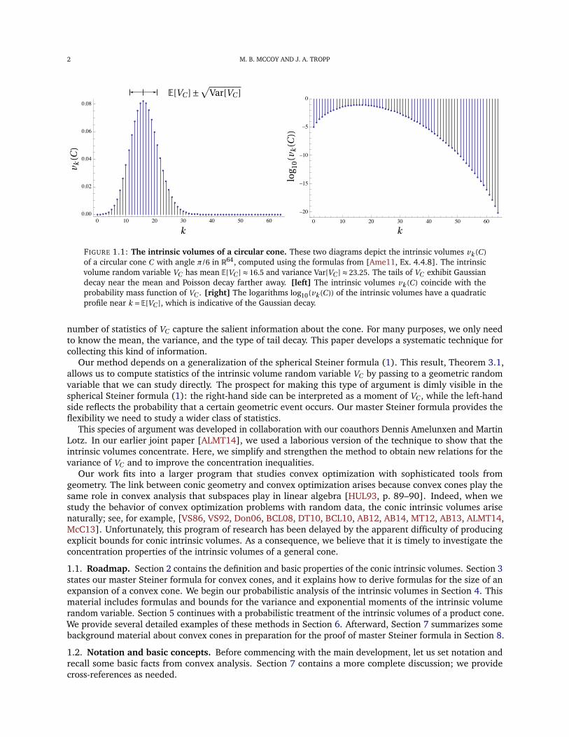
about its mean value for every closed convex cone C . In other words, most of the intrinsic volumes of a conehave negligible size; see Figure 1.1 for a typical example. As a consequence of this phenomenon, a small

Date: 23 August 2013. Revised 20 March 2014 and 29 April 2014.2010 Mathematics Subject Classification. Primary: 52A22, 60D05. Secondary: 52A20.Key words and phrases. Concentration inequality; convex cone; Gaussian width; integral geometry; intrinsic volume; geometric

probability; statistical dimension; Steiner formula; variance bound.1The j th conic intrinsic volume v j (C ) corresponds to the ( j −1)th spherical intrinsic volume ν j−1(C ∩Sd−1) that appears in the literature.

1

2 M. B. MCCOY AND J. A. TROPP

0 10 20 30 40 50 600.00

0.02

0.04

0.06

0.08

0 10 20 30 40 50 60

0

–5

–10

–15

–20

FIGURE 1.1: The intrinsic volumes of a circular cone. These two diagrams depict the intrinsic volumes vk (C )of a circular cone C with angle π/6 in R64, computed using the formulas from [Ame11, Ex. 4.4.8]. The intrinsicvolume random variable VC has mean E[VC ] ≈ 16.5 and variance Var[VC ] ≈ 23.25. The tails of VC exhibit Gaussiandecay near the mean and Poisson decay farther away. [left] The intrinsic volumes vk (C ) coincide with theprobability mass function of VC . [right] The logarithms log10(vk (C )) of the intrinsic volumes have a quadraticprofile near k = E[VC ], which is indicative of the Gaussian decay.

number of statistics of VC capture the salient information about the cone. For many purposes, we only needto know the mean, the variance, and the type of tail decay. This paper develops a systematic technique forcollecting this kind of information.

Our method depends on a generalization of the spherical Steiner formula (1). This result, Theorem 3.1,allows us to compute statistics of the intrinsic volume random variable VC by passing to a geometric randomvariable that we can study directly. The prospect for making this type of argument is dimly visible in thespherical Steiner formula (1): the right-hand side can be interpreted as a moment of VC , while the left-handside reflects the probability that a certain geometric event occurs. Our master Steiner formula provides theflexibility we need to study a wider class of statistics.

This species of argument was developed in collaboration with our coauthors Dennis Amelunxen and MartinLotz. In our earlier joint paper [ALMT14], we used a laborious version of the technique to show that theintrinsic volumes concentrate. Here, we simplify and strengthen the method to obtain new relations for thevariance of VC and to improve the concentration inequalities.

Our work fits into a larger program that studies convex optimization with sophisticated tools fromgeometry. The link between conic geometry and convex optimization arises because convex cones play thesame role in convex analysis that subspaces play in linear algebra [HUL93, p. 89–90]. Indeed, when westudy the behavior of convex optimization problems with random data, the conic intrinsic volumes arisenaturally; see, for example, [VS86, VS92, Don06, BCL08, DT10, BCL10, AB12, AB14, MT12, AB13, ALMT14,McC13]. Unfortunately, this program of research has been delayed by the apparent difficulty of producingexplicit bounds for conic intrinsic volumes. As a consequence, we believe that it is timely to investigate theconcentration properties of the intrinsic volumes of a general cone.

1.1. Roadmap. Section 2 contains the definition and basic properties of the conic intrinsic volumes. Section 3states our master Steiner formula for convex cones, and it explains how to derive formulas for the size of anexpansion of a convex cone. We begin our probabilistic analysis of the intrinsic volumes in Section 4. Thismaterial includes formulas and bounds for the variance and exponential moments of the intrinsic volumerandom variable. Section 5 continues with a probabilistic treatment of the intrinsic volumes of a product cone.We provide several detailed examples of these methods in Section 6. Afterward, Section 7 summarizes somebackground material about convex cones in preparation for the proof of master Steiner formula in Section 8.

1.2. Notation and basic concepts. Before commencing with the main development, let us set notation andrecall some basic facts from convex analysis. Section 7 contains a more complete discussion; we providecross-references as needed.

STEINER FORMULAS FOR CONES AND INTRINSIC VOLUMES 3

We work in the Euclidean space Rd , equipped with the standard inner product ⟨·, ·⟩, the associated norm‖·‖, and the norm topology. The symbols 0 and 0d refer to the origin of Rd . For a point x ∈Rd and a set K ⊂Rd ,we define the distance dist(x ,K ) := inf

{‖x − y‖ : y ∈ K}.

A convex cone C is a nonempty subset of Rd that satisfies

τ · (x + y) ∈C for all τ> 0 and x , y ∈C .

We designate the family Cd of all closed convex cones in Rd . A cone C is polyhedral if it can be expressed asthe intersection of a finite number of halfspaces:

C =N⋂

i=1

{x ∈Rd : ⟨ui , x⟩ ≥ 0

}for some ui ∈Rd .

For each cone C ∈Cd , we define the polar cone C ◦ ∈Cd via the formula

C ◦ := {u ∈Rd : ⟨u, x⟩ ≤ 0 for all x ∈C

}.

The polar of a polyhedral cone is always polyhedral.We introduce the metric projector ΠC onto a cone C ∈Cd by the formula

ΠC :Rd →C where ΠC (x) := arg min{‖x − y‖2 : y ∈C

}. (1.3)

The metric projector onto a closed convex cone is a nonnegatively homogeneous function:

ΠC (τx) = τ ·ΠC (x) for all τ≥ 0 and x ∈Rd .

The squared norm of the metric projection is a differentiable function:

∇‖ΠC (x)‖2 = 2ΠC (x) for all x ∈Rd . (1.4)

This result follows from [RW98, Thm. 2.26].We conclude with the basic notation concerning probability. We write P for the probability of an event and

E for the expectation operator. The symbol ∼ denotes equality of distribution. We reserve the letter g for astandard Gaussian vector, and θ denotes a vector uniformly distributed on the sphere. The dimensions aredetermined by context.

2. THE INTRINSIC VOLUMES OF A CONVEX CONE

We begin with an introduction to the conic intrinsic volumes that is motivated by the treatment in [Ame11].To each closed convex cone, we can assign a sequence of intrinsic volumes. For polyhedral cones, thesefunctionals have a clear geometric meaning, so we start with the definition for this special case.

Definition 2.1 (Intrinsic volumes of a polyhedral cone). Let C ∈Cd be a polyhedral cone. For k = 0,1,2, . . . ,d ,the conic intrinsic volume vk (C ) is the quantity

vk (C ) :=P{ΠC (g ) lies in the relative interior of a k-dimensional face of C

}.

The metric projector ΠC onto the cone is defined in (1.2), and the random vector g is drawn from the standardGaussian distribution on Rd .

As explained in Section 7.3, we can equip the set Cd with the conic Hausdorff metric to form a compactmetric space. The polyhedral cones form a dense subset of Cd , so it is natural to use approximation to extendthe definition of the intrinsic volumes to nonpolyhedral cones.

Definition 2.2 (Intrinsic volumes of a closed convex cone). Let C ∈Cd be a closed convex cone. Consider anysequence (Ci )i∈N of polyhedral cones in Cd where Ci →C in the conic Hausdorff metric. Define

vk (C ) := limi→∞

vk (Ci ) for k = 0,1,2, . . . ,d . (2.1)

The geometric functionals vk : Cd → [0,1] are called conic intrinsic volumes.

See Section 8.2 for a proof that the limit in (2.2) is well defined. The reader should be aware that thegeometric interpretation of intrinsic volumes from Definition 2.1 breaks down for general cones because thelimiting process does not preserve facial structure.

The conic intrinsic volumes have some remarkable properties. Fix the ambient dimension d , and let C ∈Cd

be a closed convex cone in Rd . The intrinsic volumes are...


(1) Intrinsic. The intrinsic volumes do not depend on the dimension of the space Rd in which the coneC is embedded. That is, for each natural number r ,

vk (C × {0r }) ={

vk (C ), 0 ≤ k ≤ d

0, d < k ≤ d + r.

(2) Volumes. Let γd denote the standard Gaussian measure on Rd . Then vd (C ) = γd (C ) and v0(C ) = γd (C ◦)where C ◦ denotes the polar cone. The other intrinsic volumes, however, do not admit such a clearinterpretation.

(3) Rotation invariant. For each d ×d orthogonal matrix Q, we have vk (QC ) = vk (C ).

(4) Continuous. If Ci →C in the conic Hausdorff metric, then vk (Ci ) → vk (C ).

(5) A distribution. The intrinsic volumes form a probability distribution on {0,1,2, . . . ,d}. That is,

vk (C ) ≥ 0 andd∑

j=0v j (C ) = 1.

(6) Indicators of dimension for a subspace. For any j -dimensional subspace L j ⊂Rd , we have

vk (L j ) ={

1, k = j

0, k 6= j .

(7) Reversed under polarity. The intrinsic volumes of the polar cone C ◦ satisfy

vk (C ◦) = vd−k (C ).

These claims follow from Definition 2.2 using facts from Sections 1.2 and 7 about the geometry of convexcones.

Remark 2.3 (Notation for intrinsic volumes). The notation vk for the kth intrinsic volume does not specifythe ambient dimension. This convention is justified because the intrinsic volumes of a cone do not depend onthe embedding dimension.

3. A GENERALIZED STEINER FORMULA FOR CONES

As we have seen, the intrinsic volumes of a cone form a probability distribution. Probabilistic methods offera powerful technique for studying the intrinsic volumes. To pursue this idea, we want access to momentsand other statistics of the sequence of intrinsic volumes. We acquire this information using a general Steinerformula for cones.

3.1. The master Steiner formula. Let us introduce a class of Gaussian integrals. Fix a Borel measurablebivariate function f :R2+ →R. Consider the geometric functional

ϕ f : Cd →R where ϕ f (C ) := E[f(‖ΠC (g )‖2 , ‖ΠC◦ (g )‖2 )]

. (3.1)

As usual, g ∈Rd is a standard Gaussian vector, and the expectation is interpreted as a Lebesgue integral. Wecan develop an elegant expansion of ϕ f in terms of the conic intrinsic volumes.

Theorem 3.1 (Master Steiner formula for cones). Let f : R2+ → R be a Borel measurable function. Then thegeometric functional ϕ f defined in (3.1) admits the expression

ϕ f (C ) =d∑

k=0ϕ f (Lk ) · vk (C ) for C ∈Cd (3.2)

provided that all the expectations in (3.1) are finite. Here, Lk denotes a k-dimensional subspace of Rd and theconic intrinsic volumes vk are introduced in Definition 2.2.

The coefficients ϕ f (Lk ) in the expression (3.1) have an alternative form that is convenient for computations.Let Lk be an arbitrary k-dimensional subspace of Rd . According to the definition (3.1) of the functional ϕ f ,

ϕ f (Lk ) = E[f(‖ΠLk (g )‖2 , ‖ΠLk

◦ (g )‖2 )].


The marginal property of the standard Gaussian vector g ensures that ΠLk (g ) and ΠLk◦ (g ) are independent

standard Gaussian vectors supported on Lk and Lk◦. Thus, ‖ΠLk (g )‖2 and ‖ΠLk

◦ (g )‖2 are independent chi-square random variables with k and d − k degrees of freedom respectively. Note the convention that achi-square variable with zero degrees of freedom is identically zero. In view of this fact, we have the followingequivalent of Theorem 3.1.

Corollary 3.2. Instate the hypotheses and notation of Theorem 3.1. Let{

X0, . . . , Xd}

be an independent sequenceof random variables where Xk has the chi-square distribution with k degrees of freedom, and let

{X ′

0, . . . , X ′d

}be

an independent copy of this sequence. Then

ϕ f (C ) =d∑

k=0E[

f(Xk , X ′

d−k

)] · vk (C ) for C ∈Cd .

Corollary 3.2 has an appealing probabilistic consequence. For every cone C ∈ Cd , the random variable‖ΠC (g )‖2 is a mixture of chi-square random variables X0, . . . , Xd where the mixture coefficients vk (C ) aredetermined solely by the cone. This fact corresponds with a classical observation from the field of constrainedstatistical inference, where the random variate ‖ΠC (g )‖2 is known as the chi-bar-squared statistic [SS05,Sec. 3.4].

We outline the proof of Theorem 3.1 in Sections 7 and 8. The argument involves techniques that arealready familiar to experts. Many of the core ideas appear in McMullen’s influential paper [McM75]. Asimilar approach has been used in hyperbolic integral geometry [San80, p. 242]; see also the proof of [SW08,Thm. 6.5.1]. The main technical novelty is our method for showing that the conic intrinsic volumes arecontinuous with respect to the conic Hausdorff metric.

3.2. How big is the expansion of a cone? The Euclidean Steiner formula (1) describes the volume of aEuclidean expansion of a compact convex set. Although it may not be obvious from the identity (3.1), themaster Steiner formula contains information about the volume of an expansion of a convex cone. This sectionexplains the connection, which justifies our decision to call Theorem 3.1 a Steiner formula.

First, we argue that there is a simple expression for the Gaussian measure of a Euclidean expansion of aconvex cone.

Proposition 3.3 (Gaussian Steiner formula). For each cone C ∈Cd and each number λ≥ 0,

γd (C +λBd ) =P{dist2(g ,C ) ≤λ}= d∑

k=0P{

Xd−k ≤λ} · vk (C ) (3.3)

where γd is the standard Gaussian measure on Rd and Bd is the unit ball in Rd . The random variable X j followsthe chi-square distribution with j degrees of freedom.

Proof. The first identity in (3.3) is immediate. For the second, we appeal to Corollary 3.2 with the function

f (a,b) ={

1, b ≤λ0, otherwise.

This step yields the relation

P{

dist2(g ,C ) ≤λ}=P{‖ΠC◦ (g )‖2 ≤λ}= d∑k=0

E[

f(Xk , X ′

d−k

)]= d∑k=0

P{

X ′d−k ≤λ} · vk (C ).

The first equality depends on the representation (7.1) of the distance to a cone in terms of the metric projectoronto the polar cone. The result (3.3) follows because X ′

d−k has the same distribution as Xd−k . �

We can also establish the spherical Steiner formula (1) as a consequence of Theorem 3.1 by replacing theGaussian vector g in Proposition 3.3 with a random vector θ that is uniformly distributed on the Euclideanunit sphere. This strategy leads to an expression for the proportion of the sphere subtended by an angularexpansion of the cone.

Proposition 3.4 (Spherical Steiner formula). For each cone C ∈Cd and each number λ ∈ [0,1], it holds that

P{

dist2(θ,C ) ≤λ}= d∑k=0

P{Bd−k,d ≤λ} · vk (C ). (3.4)


The random vector θ is drawn from the uniform distribution on the unit sphere Sd−1 in Rd , and the randomvariable B j ,d follows the BETA

( 12 j , 1

2 d)

distribution.

Proof. When λ= 1, both sides of (3.4) equal one. For λ< 1, we convert the spherical variable to a Gaussianusing the relation θ ∼ g /‖g‖. It follows that

P{

dist2(θ,C ) ≤λ}=P{‖ΠC◦ (g )‖2 ≤λ(1−λ)−1 · ‖ΠC (g )‖2 }.

This identity depends on the representation (7.1) of the distance, the nonnegative homogeneity of the metricprojector ΠC◦ , and the Pythagorean relation (7.1). Apply Corollary 3.2 with the function

f (a,b) ={

1, b ≤λ(1−λ)−1a

0, otherwise.

To finish, we recall the geometric interpretation [Art02] of the beta random variable: B j ,d ∼ ‖ΠL j (θ)‖2 whereL j is a j -dimensional subspace of Rd . �

Neither the Gaussian Steiner formula (3.3) nor the spherical Steiner formula (3.4) is new. The sphericalformula is classical [All48], while the Gaussian formula has antecedents in the statistics literature [SS05,Tay06]. There is novelty, however, in our method of condensing both results from the master Steinerformula (3.1).

4. PROBABILISTIC ANALYSIS OF INTRINSIC VOLUMES

In this section, we apply probabilistic methods to the conic intrinsic volumes. Our main tool is the masterSteiner formula, Theorem 3.1, which we use repeatedly to convert statements about the intrinsic volumes of acone into statements about the projection of a Gaussian vector onto the cone. We may then apply methodsfrom Gaussian analysis to study this random variable.

4.1. The intrinsic volume random variable. Definitions 2.1 and 2.2 make it clear that the intrinsic volumesform a probability distribution. This observation suggests that it would be fruitful to analyze the intrinsicvolumes using techniques from probability. We begin with the key definition.

Definition 4.1 (Intrinsic volume random variable). Let C ∈Cd be a closed convex cone. The intrinsic volumerandom variable VC has the distribution

P{VC = k

}= vk (C ) for k = 0,1,2, . . . ,d .

Notice that the intrinsic volume random variable of a cone C ∈Cd and its polar have a tight relationship:

P{VC◦ = k

}= vk (C ◦) = vd−k (C ) =P{VC = d −k

}because polarity reverses the sequence of intrinsic volumes. In other words, VC◦ ∼ d −VC .

4.2. The statistical dimension of a cone. The expected value of the intrinsic volume random variable VC

has a distinguished place in the theory because VC concentrates sharply about this point. In anticipation ofthis result, we glorify the expectation of VC with its own name and notation.

Definition 4.2 (Statistical dimension [ALMT14, Sec. 5.3]). The statistical dimension δ(C ) of a cone C ∈Cd isthe quantity

δ(C ) := E[VC ] =d∑

k=0k vk (C ).

The statistical dimension of a cone really is a measure of its dimension. In particular,

δ(L) = dim(L) for each subspace L ⊂Rd . (4.1)

In fact, the statistical dimension is the canonical extension of the dimension of a subspace to the class ofconvex cones [ALMT14, Sec. 5.3]. By this, we mean that the statistical dimension is the only rotation invariant,continuous, localizable valuation on Cd that satisfies (4.2). See [SW08, p. 254 and Thm. 6.5.4] for furtherinformation about the unexplained technical terms.

The statistical dimension interacts beautifully with the polarity operation. In particular,

δ(C )+δ(C ◦) = E[VC ]+E[VC◦ ] = E[VC ]+E[d −VC ] = d .


This formula allows us to evaluate the statistical dimension for an important class of cones. A closed convexcone C is self-dual when it satisfies the identity C = −C ◦. Examples include the nonnegative orthant, thesecond-order cone, and the cone of positive-semidefinite matrices. We have the identity

δ(C ) = 12 d for a self-dual cone C ∈Cd . (4.2)

The statistical dimension of a cone can be expressed in terms of the projection of a standard Gaussianvector onto the cone [ALMT14, Prop. 5.11]. The master Steiner formula gives an easy proof of this result.

Proposition 4.3 (Statistical dimension). Let C ∈Cd be a closed convex cone. Then

δ(C ) = E[‖ΠC (g )‖2 ].

The identity in Proposition 4.3 can be used to evaluate the statistical dimension for many cones of interest.See [ALMT14, Sec. 4] for details and examples.

Proof. The master Steiner formula, Corollary 3.2, with function f (a,b) = a states that

E[‖ΠC (g )‖2 ]= d∑

k=0E[Xk ] · vk (C ) =

d∑k=0

k vk (C ) = δ(C ).

Indeed, a chi-square variable Xk with k degrees of freedom has expectation k. �

4.3. The variance of the intrinsic volumes. The variance of the intrinsic volume random variable tells ushow tightly the intrinsic volumes cluster around their mean value. We can find an explicit expression for thevariance in terms of the projection of a Gaussian vector onto the cone.

Proposition 4.4 (Variance of the intrinsic volumes). Let C ∈Cd be a closed convex cone. Then

Var[VC ] = Var[‖ΠC (g )‖2 ]−2δ(C ) (4.3)

= Var[‖ΠC◦ (g )‖2 ]−2δ(C ◦) = Var[VC◦ ]. (4.4)

Proposition 4.4 leads to exact formulas for the variance of the intrinsic volume sequence in severalinteresting cases; Section 6 contains some worked examples.

Proof. By definition, the variance satisfies

Var[VC ] = E[V 2

C

]− (E[VC ]

)2 = E[V 2

C

]−δ(C )2.

To obtain the expectation of V 2C , we invoke the master Steiner formula, Corollary 3.2, with the function

f (a,b) = a2 to obtain

E[‖ΠC (g )‖4 ]= d∑

k=0E[

X 2k

] · vk (C ) =d∑

k=0k2vk (C )+2

d∑k=0

k vk (C ) = E[V 2

C

]+2δ(C ).

Indeed, the raw second moment of a chi-square random variable Xk with k degrees of freedom equals k2 +2k.Combine these two displays to reach

Var[VC ] = E[‖ΠC (g )‖4 ]−δ(C )2 −2δ(C ) = E[‖ΠC (g )‖4 ]− (E[‖ΠC (g )‖2 ])2 −2δ(C )

where the second identity follows from Proposition 4.3. Identify the variance of ‖ΠC (g )‖2 to complete theproof of (4.4). To establish (4.4), note that Var[VC ] = Var[d −VC ] = Var[VC◦ ], and then apply (4.4) to therandom variable VC◦ . �

4.4. A bound for the variance of the intrinsic volumes. Proposition 4.4 also allows us to produce a generalbound on the variance of the intrinsic volumes of a cone.

Theorem 4.5 (Variance bound for intrinsic volumes). Let C ∈Cd be a closed convex cone. Then

Var[VC ] ≤ 2(δ(C )∧δ(C ◦)

).

The operator ∧ returns the minimum of two numbers.

The example in Section 6.3 demonstrates that the constant two in (4.5) cannot be reduced in general.


Proof. To bound the variance of VC , we plan to invoke the Gaussian Poincaré inequality [Bog98, Thm. 1.6.4]to control the variance of ‖ΠC (g )‖2. This inequality states that

Var[H(g )] ≤ E[‖∇H(g )‖2 ]for any function H :Rd →R whose gradient is square-integrable with respect to the standard Gaussian measure.We apply this result to the function

H(x) = ‖ΠC (x)‖2 with ‖∇H(x)‖2 = 4‖ΠC (x)‖2 .

The gradient calculation is justified by (1.2). We determine that

Var[‖ΠC (g )‖2 ]≤ 4E

[‖ΠC (g )‖2 ]= 4δ(C )

where the second identity follows from Proposition 4.3. Introduce this inequality into (4.4) to see thatVar[VC ] ≤ 2δ(C ). We can apply the same argument to see that

Var[‖ΠC◦ (g )‖2 ]≤ 4δ(C ◦).

Substitute this bound into (4.4) to conclude that Var[VC ] ≤ 2δ(C ◦). �

In principle, a random variable taking values in {0,1,2, . . . ,d} can have variance larger than d 2/3—considerthe uniform random variable. In contrast, Theorem 4.5 tells us that the variance of the intrinsic volumerandom variable VC cannot exceed d for any cone C . This observation has consequences for the tail behaviorof VC . Indeed, Chebyshev’s inequality implies that

P{|VC −δ(C )| >λ

√δ(C )

}≤ Var[VC ]

λ2δ(C )≤ 2

λ2 .

That is, most of the mass of VC is located near the statistical dimension.

4.5. Exponential moments of the intrinsic volumes. In the previous section, we discovered that theintrinsic volume random variable VC is often close to its mean value. This observation suggests that VC

might exhibit stronger concentration. A standard method for proving concentration inequalities for a randomvariable is to calculate its exponential moments. The master Steiner formula allows us to accomplish this task.

Proposition 4.6 (Exponential moments of the intrinsic volumes). Let C ∈Cd be a closed convex cone. For eachparameter η ∈R,

EeηVC = Eeξ‖ΠC (g )‖2where ξ= 1

2

(1−e−2η).

Proof. Fix a number ξ< 12 . With the choice f (a,b) = eξa , Corollary 3.2 shows that

Eeξ‖ΠC (g )‖2 =d∑

k=0E[eξXk

] · vk (C ) =d∑

k=0(1−2ξ)−k/2vk (C ) =

d∑k=0

eηk vk (C ) = EeηVC .

We have used the familiar formula for the exponential moments of a chi-square random variable Xk with kdegrees of freedom. The penultimate identity follows from the change of variables η=− 1

2 log(1−2ξ), whichestablishes a bijection between ξ< 1

2 and η ∈R. �

Remark 4.7 (Conic Wills functional). Proposition 4.6 leads to a geometric description of the generatingfunction of the intrinsic volumes:

WC (λ) :=λd Eexp

(1−λ2

2·dist2(g ,C )

)=

d∑k=0

λk vk (C ) for λ> 0. (4.5)

To see why this is true, use the representation (7.1) of the distance, and apply Proposition 4.6 with η=− logλto confirm that

WC (λ) =λd Eexp

(1−λ2

2· ‖ΠC◦ (g )‖2

)=λd

d∑k=0

λ−k vk (C ◦) =d∑

k=0λk vk (C ).

We have applied the fact that polarity reverses intrinsic volumes to reindex the sum. The function WC can beviewed as a conic analog of the Wills functional [Wil73] from Euclidean geometry.


4.6. A bound for the exponential moments of the intrinsic volumes. Proposition 4.6 allows us to obtainan excellent bound for the exponential moments of VC . In the next section, we use this result to developconcentration inequalities for the intrinsic volumes.

Theorem 4.8 (Exponential moment bound for intrinsic volumes). Let C ∈Cd be a closed convex cone. For eachparameter η ∈R,

Eeη(VC−δ(C )) ≤ exp

(e2η−2η−1

2·δ(C )

), and (4.6)


(e−2η+2η−1

2·δ(C ◦)

). (4.7)

The major technical challenge is to bound the exponential moments of the random variable ‖ΠC (g )‖2.The following lemma provides a sharp estimate for the exponential moments. It improves on an earlierresult [ALMT14, Sublem. D.3].

Lemma 4.9. Let C ∈Cd be a closed convex cone. For each parameter ξ< 12 ,

Eeξ (‖ΠC (g )‖2−δ(C )) ≤ exp

(2ξ2δ(C )

1−2ξ

).

Proof. Define the zero-mean random variable

Z := ‖ΠC (g )‖2 −δ(C ).

Introduce the moment generating function m(ξ) := EeξZ . Our aim is to bound m(ξ). Before we begin,it is helpful to note a few properties of the moment generating function. First, the derivative m′(ξ) =E[

Z eξZ]

whenever ξ < 12 . By direct calculation, logm(0) = 0. Furthermore, l’Hôpital’s rule shows that

limξ→0 ξ−1 logm(ξ) = 0 because the random variable Z has zero mean.

The argument is based on the Gaussian logarithmic Sobolev inequality [Bog98, Thm. 1.6.1]. One versionof this result states that

E[H(g ) ·eH(g )]−E[

eH(g )] log E[eH(g )]≤ 1

2E[‖∇H(g )‖2 ·eH(g )] (4.8)

for any differentiable function H :Rd →R such that the expectations in (4.6) are finite. We apply this result tothe function

H(x) = ξ [‖ΠC (x)‖2 −δ(C )]

with ‖∇H(x)‖2 = 4ξ2 ‖ΠC (x)‖2 .

The gradient calculation is justified by (1.2). Notice that

H(g ) = ξZ and ‖∇H(g )‖2 = 4ξ2(Z +δ(C )).

Therefore, the logarithmic Sobolev inequality (4.6) delivers the relation

ξ ·E[Z eξZ ]−E[

eξZ ]log E

[eξZ ]≤ 2ξ2 ·E[

Z eξZ ]+2ξ2δ(C ) ·E[eξZ ]

for ξ< 12 .

We can rewrite the last display as a differential inequality for the moment generating function:

ξm′(ξ)−m(ξ) logm(ξ) ≤ 2ξ2m′(ξ)+2δ(C ) ·ξ2m(ξ) for ξ< 12 . (4.9)

The requirement on ξ is necessary and sufficient to ensure that m(ξ) and m′(ξ) are finite. To complete theproof, we just need to solve this differential inequality.

We follow the argument from [BLM03, Thm. 5]. Divide the inequality (4.6) by the positive number ξ2m(ξ)to reach

1

ξ· m′(ξ)

m(ξ)− 1

ξ2 logm(ξ) ≤ 2 · m′(ξ)

m(ξ)+2δ(C ) for ξ ∈ (−∞,0)∪ (

0, 12

).

The left- and right-hand sides of this relation are exactly integrable:d

ds

[1

slogm(s)

]≤ 2 · d

ds

[logm(s)+2δ(C ) · s

]for s ∈ (−∞,0)∪ (

0, 12

). (4.10)

To continue, we first consider the case 0 < ξ< 12 . Integrate the inequality (4.6) over the interval s ∈ [0,ξ] using

the boundary conditions logm(0) = 0 and limξ→0 ξ−1 logm(ξ) = 0. This step yields

1

ξlogm(ξ) ≤ 2logm(ξ)+2δ(C ) ·ξ for 0 < ξ< 1

2 .


Solve this relation for the moment generating function m to obtain the bound

m(ξ) ≤ exp

(2ξ2δ(C )

1−2ξ

)for 0 ≤ ξ< 1

2 . (4.11)

The boundary case ξ = 0 follows from a direct calculation. Next, we address the situation where ξ < 0.Integrating (4.6) over the interval [ξ,0], we find that

−1

ξlogm(ξ) ≤−2logm(ξ)−2δ(C ) ·ξ for ξ< 0.

Solve this inequality for m(ξ) to see that the bound (4.6) also holds in the range ξ < 0. This observationcompletes the proof. �

With Lemma 4.9 at hand, we quickly reach Theorem 4.8.

Proof of Theorem 4.8. We begin with the statement from Proposition 4.6. Adding and subtracting multiples ofδ(C ) in the exponent, we obtain the relation

Eeη(VC−δ(C )) = e(ξ−η)δ(C ) ·Eeξ (‖ΠC (g )‖2−δ(C )).

where ξ= 12

(1−e−2η

)< 12 . Lemma 4.9 controls the moment generating function on the right-hand side:

Eeη(VC−δ(C )) ≤ e(ξ−η)δ(C ) ·exp

(2ξ2δ(C )

1−2ξ

).

By a marvelous coincidence, the terms in the exponent collapse into a compact form:

ξ−η+ 2ξ2

1−2ξ= e2η−2η−1

2.

Combine the last two displays to finish the proof of (4.8). To obtain the second formula (4.8), note that

Eeη(VC−δ(C )) = Ee(−η)(VC◦−δ(C◦))

because VC ∼ d −VC◦ and δ(C ) = d −δ(C ◦). Now apply (4.8) to the right-hand side. �

4.7. Concentration of intrinsic volumes. The exponential moment bound from Theorem 4.8 allows us toobtain concentration results for the sequence of intrinsic volumes of a convex cone. The following corollaryprovides Bennett-type inequalities for the intrinsic volume random variable.

Corollary 4.10 (Concentration of the intrinsic volume random variable). Let C ∈Cd be a closed convex cone.For each λ≥ 0, the intrinsic volume random variable VC satisfies the upper tail bound

P{VC −δ(C ) ≥λ}≤ exp

(−1

2max

{δ(C ) ·ψ

(λ

δ(C )

), δ(C ◦) ·ψ

( −λδ(C ◦)

)})(4.12)

and the lower tail bound

P{VC −δ(C ) ≤−λ}≤ exp

(−1

2max

{δ(C ) ·ψ

( −λδ(C )

), δ(C ◦) ·ψ

(λ

δ(C ◦)

)}). (4.13)

The function ψ(u) := (1+u) log(1+u)−u for u ≥−1 while ψ(u) =∞ for u <−1.

Proof. The argument, based on the Laplace transform method, is standard. For any η> 0,

P{VC −δ(C ) ≥λ}≤ e−ηλ ·Eeη (VC−δ(C )) ≤ e−ηλ ·exp

(e2η−2η−1

2·δ(C )

)where we have applied the exponential moment bound (4.8) from Theorem 4.8. Minimize the right-hand sideover η> 0 to obtain the first branch of the maximum in (4.10). The second exponential moment bound (4.8)leads to the second branch of the maximum in (4.10). The lower tail bound (4.10) follows from the sameconsiderations. For more details about this type of proof, see [BLM13, Sec. 2.7]. �


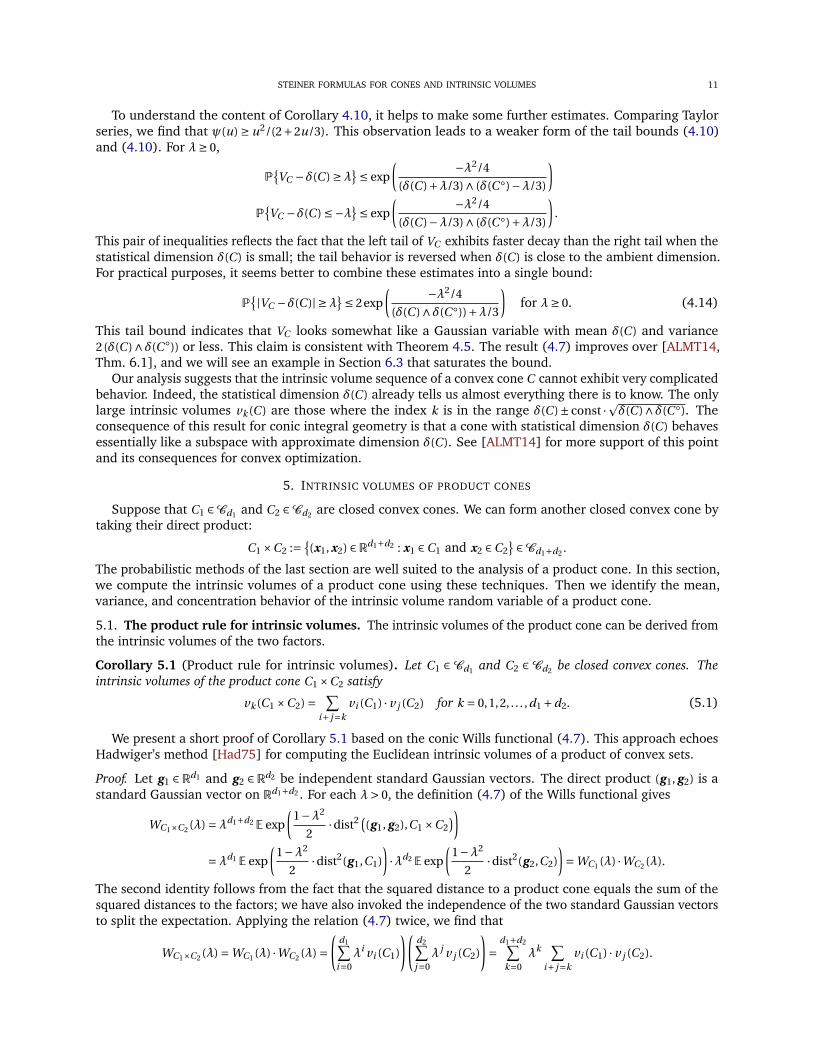
To understand the content of Corollary 4.10, it helps to make some further estimates. Comparing Taylorseries, we find that ψ(u) ≥ u2/(2+2u/3). This observation leads to a weaker form of the tail bounds (4.10)and (4.10). For λ≥ 0,

P{VC −δ(C ) ≥λ}≤ exp

( −λ2/4

(δ(C )+λ/3)∧ (δ(C ◦)−λ/3)

)P{VC −δ(C ) ≤−λ}≤ exp

( −λ2/4

(δ(C )−λ/3)∧ (δ(C ◦)+λ/3)

).

This pair of inequalities reflects the fact that the left tail of VC exhibits faster decay than the right tail when thestatistical dimension δ(C ) is small; the tail behavior is reversed when δ(C ) is close to the ambient dimension.For practical purposes, it seems better to combine these estimates into a single bound:

P{ |VC −δ(C )| ≥λ}≤ 2exp

( −λ2/4

(δ(C )∧δ(C ◦))+λ/3

)for λ≥ 0. (4.14)

This tail bound indicates that VC looks somewhat like a Gaussian variable with mean δ(C ) and variance2(δ(C )∧δ(C ◦)) or less. This claim is consistent with Theorem 4.5. The result (4.7) improves over [ALMT14,Thm. 6.1], and we will see an example in Section 6.3 that saturates the bound.

Our analysis suggests that the intrinsic volume sequence of a convex cone C cannot exhibit very complicatedbehavior. Indeed, the statistical dimension δ(C ) already tells us almost everything there is to know. The onlylarge intrinsic volumes vk (C ) are those where the index k is in the range δ(C )± const ·pδ(C )∧δ(C ◦). Theconsequence of this result for conic integral geometry is that a cone with statistical dimension δ(C ) behavesessentially like a subspace with approximate dimension δ(C ). See [ALMT14] for more support of this pointand its consequences for convex optimization.

5. INTRINSIC VOLUMES OF PRODUCT CONES

Suppose that C1 ∈Cd1 and C2 ∈Cd2 are closed convex cones. We can form another closed convex cone bytaking their direct product:

C1 ×C2 := {(x1, x2) ∈Rd1+d2 : x1 ∈C1 and x2 ∈C2

} ∈Cd1+d2 .

The probabilistic methods of the last section are well suited to the analysis of a product cone. In this section,we compute the intrinsic volumes of a product cone using these techniques. Then we identify the mean,variance, and concentration behavior of the intrinsic volume random variable of a product cone.

5.1. The product rule for intrinsic volumes. The intrinsic volumes of the product cone can be derived fromthe intrinsic volumes of the two factors.

Corollary 5.1 (Product rule for intrinsic volumes). Let C1 ∈ Cd1 and C2 ∈ Cd2 be closed convex cones. Theintrinsic volumes of the product cone C1 ×C2 satisfy

vk (C1 ×C2) = ∑i+ j=k

vi (C1) · v j (C2) for k = 0,1,2, . . . ,d1 +d2. (5.1)

We present a short proof of Corollary 5.1 based on the conic Wills functional (4.7). This approach echoesHadwiger’s method [Had75] for computing the Euclidean intrinsic volumes of a product of convex sets.

Proof. Let g1 ∈ Rd1 and g2 ∈ Rd2 be independent standard Gaussian vectors. The direct product (g1, g2) is astandard Gaussian vector on Rd1+d2 . For each λ> 0, the definition (4.7) of the Wills functional gives

WC1×C2 (λ) =λd1+d2 E exp

(1−λ2

2·dist2 (

(g1, g2),C1 ×C2))

=λd1 E exp

(1−λ2

2·dist2(g1,C1)

)·λd2 E exp

(1−λ2

2·dist2(g2,C2)

)=WC1 (λ) ·WC2 (λ).

The second identity follows from the fact that the squared distance to a product cone equals the sum of thesquared distances to the factors; we have also invoked the independence of the two standard Gaussian vectorsto split the expectation. Applying the relation (4.7) twice, we find that

WC1×C2 (λ) =WC1 (λ) ·WC2 (λ) =(

d1∑i=0

λi vi (C1)

)(d2∑

j=0λ j v j (C2)

)=

d1+d2∑k=0

λk∑

i+ j=kvi (C1) · v j (C2).


But (4.7) also shows that

WC1×C2 (λ) =d1+d2∑

k=0λk vk (C1 ×C2).

Comparing coefficients in these two polynomials, we arrive at the relation (5.1). �

5.2. Concentration of the intrinsic volumes of a product cone. We can employ the probabilistic techniquesfrom Section 4 to collect information about the intrinsic volumes of a product cone. Let C1 ∈Cd1 and C2 ∈Cd2

be two cones, and consider independent random variables VC1 and VC2 whose distributions are given by theintrinsic volumes of C1 and C2. In view of Corollary 5.1,

vk (C1 ×C2) = ∑i+ j=k

vi (C1) · v j (C2) =P{VC1 +VC2 = k

}for k = 0,1,2, . . . ,d1 +d2.

In other words, the intrinsic volume random variable VC1×C2 of the product cone has the distribution

VC1×C2 ∼VC1 +VC2 . (5.2)

This observation allows us to compute the statistical dimension of the product cone:

δ(C1 ×C2) = E[VC1×C2

]= δ(C1)+δ(C2). (5.3)

Of course, we can also derive (5.2) directly from Proposition 4.3. A more interesting consequence is thefollowing expression for the variance of the intrinsic volumes:

Var[VC1×C2

]= Var[VC1 ]+Var[VC2 ] ≤ 2[(δ(C1)∧δ(C ◦

1))+ (

δ(C2)∧δ(C ◦2)

)]. (5.4)

The inequality follows from Theorem 4.5. With some additional effort, we can develop a concentration resultfor the intrinsic volumes of a product cone that matches the variance bound (5.2).

Corollary 5.2 (Concentration of intrinsic volumes for a product cone). Let C1 ∈Cd1 and C2 ∈Cd2 be closedconvex cones. For each λ≥ 0,

P{∣∣VC1×C2 −δ(C1 ×C2)

∣∣≥λ}≤ 2 exp

( −λ2/4

σ2 +λ/3

)where σ2 := (

δ(C1)∧δ(C ◦1)

)+ (δ(C2)∧δ(C ◦

2)).

This represents a significant improvement over the simple tail bound from [ALMT14, Lem. 7.2]. A similarresult holds for any finite product C1 ×·· ·×Cr of closed convex cones.

Proof. First, recall the numerical inequality

e2η−2η−1

2≤ η2

1−2 |η|/3for |η| < 3

2 .

This estimate allows us to package the two exponential moment bounds from Theorem 4.8 as


(η2(δ(C )∧δ(C ◦))

1−2 |η|/3

)for |η| < 3

2 .

Applying this bound twice, we learn that the exponential moments of the random variable VC1×C2 satisfy

Eeη (VC1×C2−δ(C1×C2)) = Eeη (VC1−δ(C1)) ·Eeη (VC2−δ(C2)) ≤ exp

(η2σ2

1−2 |η|/3

).

The first relation follows from the distributional identity (5.2) and the statistical dimension calculation (5.2).The Laplace transform method delivers

P{VC1×C2 −δ(C1 ×C2) ≥λ}≤ inf

η>0

{e−ηλ ·exp

(η2σ2

1−2 |η|/3

)}≤ exp

( −λ2/4

σ2 +λ/3

).

We have chosen η=λ/(2σ2 +2λ/3) to reach the second inequality. We obtain the lower tail bound from thesame argument. �

6. EXAMPLES

In this section, we demonstrate the vigor of the ideas from Section 4 by applying them to some concreteexamples. The probabilistic viewpoint provides new insights, and it enables us to complete some difficultcalculations with minimal effort.


6.1. The nonnegative orthant. As a warmup, we begin with an example where it is easy to compute theintrinsic volumes directly. The nonnegative orthant Rd+ is the polyhedral cone

Rd+ := {

x ∈Rd : xi ≥ 0 for i = 1, . . . ,d .}.

The nonnegative orthant is self-dual, which immediately delivers several results. For typographical felicity, weabbreviate C =Rd+. Applying the identity (4.2) and Theorem 4.5, we find that

δ(C ) = E[VC ] = 12 d and Var[VC ] ≤ 2δ(C ) = d .

The tail bound (4.7) specializes to

P{∣∣VC − 1

2 d∣∣≥λ}≤ 2 exp

( −λ2

2d +4λ/3

).

These estimates already provide a significant amount of information about the intrinsic volumes of the orthant.How well do these bounds describe the actual behavior of the intrinsic volumes? Appealing directly to

Definition 2.1, we can check that VC ∼ BINOMIAL(d , 1

2

). See, for example, [Ame11, Ex. 4.4.7]. Therefore,

E[VC ] = 12 d and Var[VC ] = 1

4 d .

Furthermore, the binomial random variable satisfies a sharp tail bound of the form

P{∣∣VC − 1

2 d∣∣≥λ}≤ 2 exp

(−2λ2

d

).

We discover that our general results overestimate the variance of VC by a factor of four, but they do capturethe subgaussian decay of the intrinsic volumes.

6.2. The cone of positive-semidefinite matrices. Our approach to intrinsic volume calculations is mostvaluable when there is no explicit formula for the intrinsic volumes or the expressions are too complicated toevaluate easily. For a challenge of this type, let us consider the cone of real positive-semidefinite matrices. Wecan compute the mean and variance of the intrinsic volume sequence of this cone by combining our methodswith established results from random matrix theory.

The cone Sn+ consists of all n ×n positive-semidefinite (psd) matrices:

Sn+ := {

X ∈Rn×nsym : uT X u ≥ 0 for all u ∈Rn}

where Rn×nsym consists of n ×n symmetric matrices. This vector space has dimension d = n(n +1)/2. The psd

cone is self-dual with respect to Rn×nsym , so the expression (4.2) shows that the statistical dimension

δ(Sn+) = n(n +1)

4.

As with the nonnegative orthant, we immediately obtain bounds on the variance and concentration inequalitiesfor the intrinsic volumes.

We will use Proposition 4.4 to compute the variance of the sequence of intrinsic volumes when n is large.Let us abbreviate C =Sn+. The intrinsic volumes do not depend on the embedding dimension of the cone, sothere is no harm in treating the cone as a subset of the linear space Rn×n of square matrices. To compute themetric projection of a matrix X ∈Rn×n onto the cone C , we first extract the symmetric part of the matrix andthen compute the positive part [Bha97, p. 99] of the Jordan decomposition:

ΠC (X ) =ΠC( 1

2 (X +X T ))= 1

2 (X +X T )+.

It follows that‖ΠC (X )‖2

F = 14

∥∥(X +X T )

+∥∥2

F = 14 tr

[(X +X T )2

+].

Let Gn ∈Rn×n be a matrix with independent standard Gaussian entries. Then the matrix Wn = 2−1/2(Gn +GT

n

) ∈Rn×n

sym is a member of the Gaussian orthogonal ensemble (GOE). We have

‖ΠC (Gn)‖2F = 1

2 tr[(Wn)2

+].

To invoke Proposition 4.4, we must compute the variance of this quantity.Our method is to renormalize the matrix and invoke asymptotic results for the GOE. From the formula

above,

Var[‖ΠC (Gn)‖2

F

]= Var[n

2· tr

[(n−1/2Wn

)2+]]= n2

4Var

[1

ntr

[(Wn

)2+]]

.


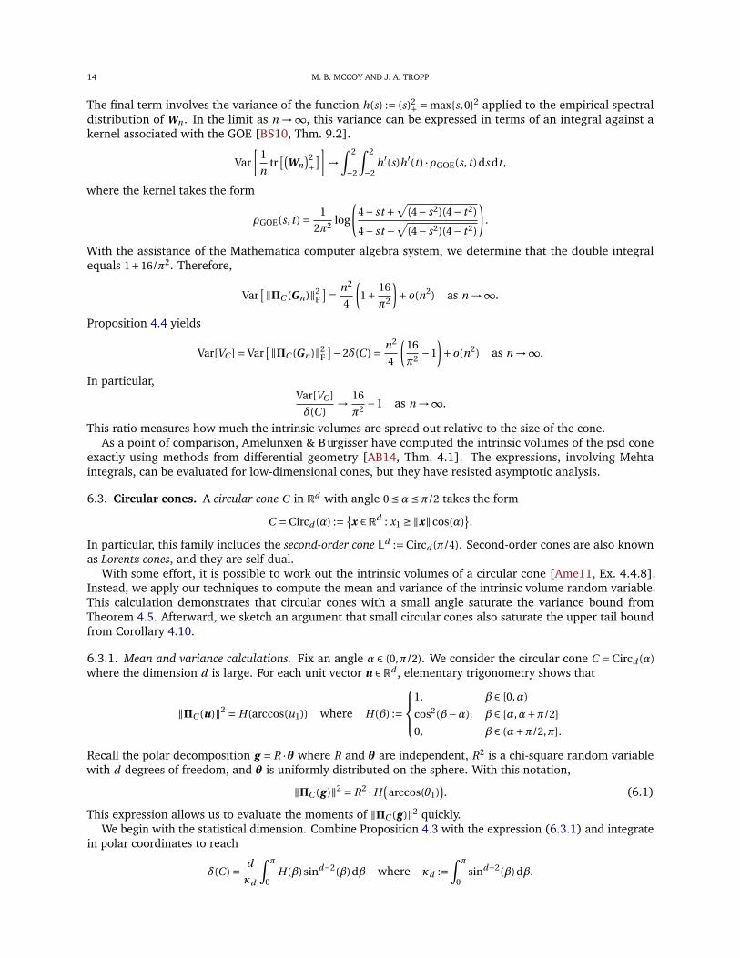
The final term involves the variance of the function h(s) := (s)2+ = max{s,0}2 applied to the empirical spectraldistribution of Wn . In the limit as n →∞, this variance can be expressed in terms of an integral against akernel associated with the GOE [BS10, Thm. 9.2].

Var

[1

ntr

[(Wn

)2+]]→

∫ 2

−2

∫ 2

−2h′(s)h′(t ) ·ρGOE(s, t )ds dt ,

where the kernel takes the form

ρGOE(s, t ) = 1

2π2 log

(4− st +

√(4− s2)(4− t 2)

4− st −√

(4− s2)(4− t 2)

).

With the assistance of the Mathematica computer algebra system, we determine that the double integralequals 1+16/π2. Therefore,

Var[‖ΠC (Gn)‖2

F

]= n2

4

(1+ 16

π2

)+o(n2) as n →∞.

Proposition 4.4 yields

Var[VC ] = Var[‖ΠC (Gn)‖2

F

]−2δ(C ) = n2

4

(16

π2 −1

)+o(n2) as n →∞.

In particular,Var[VC ]

δ(C )→ 16

π2 −1 as n →∞.

This ratio measures how much the intrinsic volumes are spread out relative to the size of the cone.As a point of comparison, Amelunxen & Bürgisser have computed the intrinsic volumes of the psd cone

exactly using methods from differential geometry [AB14, Thm. 4.1]. The expressions, involving Mehtaintegrals, can be evaluated for low-dimensional cones, but they have resisted asymptotic analysis.

6.3. Circular cones. A circular cone C in Rd with angle 0 ≤α≤π/2 takes the form

C = Circd (α) := {x ∈Rd : x1 ≥ ‖x‖cos(α)

}.

In particular, this family includes the second-order cone Ld := Circd (π/4). Second-order cones are also knownas Lorentz cones, and they are self-dual.

With some effort, it is possible to work out the intrinsic volumes of a circular cone [Ame11, Ex. 4.4.8].Instead, we apply our techniques to compute the mean and variance of the intrinsic volume random variable.This calculation demonstrates that circular cones with a small angle saturate the variance bound fromTheorem 4.5. Afterward, we sketch an argument that small circular cones also saturate the upper tail boundfrom Corollary 4.10.

6.3.1. Mean and variance calculations. Fix an angle α ∈ (0,π/2). We consider the circular cone C = Circd (α)where the dimension d is large. For each unit vector u ∈Rd , elementary trigonometry shows that

‖ΠC (u)‖2 = H(arccos(u1)) where H(β) :=

1, β ∈ [0,α)

cos2(β−α), β ∈ [α,α+π/2]

0, β ∈ (α+π/2,π].

Recall the polar decomposition g = R ·θ where R and θ are independent, R2 is a chi-square random variablewith d degrees of freedom, and θ is uniformly distributed on the sphere. With this notation,

‖ΠC (g )‖2 = R2 ·H(

arccos(θ1)). (6.1)

This expression allows us to evaluate the moments of ‖ΠC (g )‖2 quickly.We begin with the statistical dimension. Combine Proposition 4.3 with the expression (6.3.1) and integrate

in polar coordinates to reach

δ(C ) = d

κd

∫ π

0H(β)sind−2(β)dβ where κd :=

∫ π

0sind−2(β)dβ.


A more detailed version of this calculation appears in [McC13, Prop. 6.8]. The function β 7→ sind−2(β) peakssharply around π/2, so it does little harm to replace H by the function H̃(β) = cos2(β−α) in the integrand.Computing this simpler integral, we obtain a closed-form expression plus a remainder term:

δ(C ) = d sin2(α)+cos(2α)+ε1(α,d). (6.2)

We assert that the remainder term is exponentially small as a function of the dimension:

|ε1(α,d)| <√π

8·d 3/2 ·exp

(−1

2(d −1) · (α∧ (π/2−α)

)2)

.

The precise form of the error is not particularly important here, so we omit the details.The same approach delivers the variance of VC . Repeating the argument above, we get

E[‖ΠC (g )‖4 ]= d(d +2)

κd

∫ π

0H(β)2 sind−2(β)dβ.

Replace H with H̃ and integrate to obtain

E[‖ΠC (g )‖4 ]= 3

8 d(d +2)−4(d −2)(d +2)cos(2α)− (d −4)(d −2)cos(4α)+ε2(α,d). (6.3)

The error term satisfies the bound

|ε2(α,d)| ≤√π

8·d 3/2(d +2) ·exp

(−1

2(d −1) · (α∧ (π/2−α)

)2)

.

In view of Proposition 4.3 and Proposition 4.4, we determine that

Var[VC ] = Var[‖ΠC (g )‖2 ]−2δ(C ) = E[‖ΠC (g )‖4 ]−δ(C )2 −2δ(C ). (6.4)

Combine (6.3.1), (6.3.1), and (6.3.1) and simplify to reach

Var[VC ] = 12 (d −2)sin2(2α)+ε3(α,d).

Once again, the remainder term is exponentially small in the dimension d for each fixed α ∈ (0,π/2).These calculations allow us to compare the variance of VC with the statistical dimension δ(C ):

Var[VC ]

δ(C )= (d −2)sin2(2α)

2d sin2(α)+ε4(α,d) → 2cos2(α) as d →∞ with fixed α> 0.

By considering a sufficiently small angle α, we can find a circular cone C = Circd (α) for which Var[VC ] isarbitrarily close to 2δ(C ). In conclusion, we cannot improve the constant two in the variance bound fromTheorem 4.5.

6.3.2. Tail behavior. Circular cones also exhibit tail behavior that matches the predictions of Corollary 4.10exactly. It takes some technical effort to establish this claim in detail, so we limit ourselves to a sketch of theargument. These ideas are drawn from [ALMT14, Sec. 6.2].

Fix an angle 0 < α¿ π2 , and abbreviate q = sin2(α). Consider the circular cone C = Circd (α) where the

dimension takes the form d = 2(n +1) where n is a large integer. In particular, the formula (6.3.1) showsthat the statistical dimension δ(C ) ≈ d sin2(α) ≈ 2nq. It can be established that the odd intrinsic volumes of Cfollow a binomial distribution [Ame11, Ex. 4.4.8]:

2 v2k+1(C ) =P{Y = k} where Y = Yn ∼ BINOMIAL(n, q).

As a consequence of the Gauss–Bonnet Theorem [SW08, Thm. 6.5.5], there is an interlacing result [ALMT14,Prop. 5.6] for the upper tail of VC .

P{Y ≥ k

}≤P{VC ≥ 2k

}≤P{Y ≥ k −1

}.

Thus, accurate probability bounds for VC follow from bounds for the binomial random variable Y .Our tail inequality, Corollary 4.10, predicts that VC has subgaussian behavior for moderate deviations. To

see that circular cones actually display this behavior, we turn to the classical limits for the binomial randomvariable Yn . The Laplace–de Moivre central limit theorem states that

P{Yn −nq ≥ t

√nq(1−q)

}→ 1−Φ(t ) as n →∞ with q fixed.

Here, Φ denotes the distribution function of a standard Gaussian variate. When q ≈ 0 and n is large, we caninvoke the approximation δ(C ) ≈ 2nq and a tail bound for the Gaussian distribution to obtain

P{VC −δ(C ) ≥λ

√δ(C )

}≈P{VC −2nq ≥λ√

2nq(1−q)}≈P{

Yn −nq ≥ (2−1/2λ)√

nq(1−q)}≈ e−λ

2/4.


TABLE 6.1: Statistical dimension and variance calculations. This table lists the statistical dimension δ(C ) andthe variance Var[VC ] for several families of convex cones. The last column displays the limiting ratio Var[VC ]/δ(C )as the dimensional parameter tends to infinity.

Cone Notation Mean δ(C ) Variance Var[VC ] Limit of Var[VC ]/δ(C )

Subspace Lk k 0 0

Nonnegative orthant Rd+12 d 1

4 d 12

Real positive-semidefinite cone Sn+14 n(n +1) ≈ ( 4

π2 − 14

)n2 16

π2 −1

Second-order cone Ld 12 d ≈ 1

2 (d −2) 1

Circular cone Circd (α) ≈ d sin2(α) ≈ 12 (d −2)sin2(2α) 2cos2(α)

Upper bound (Theorem 4.5) 2

This expression matches the behavior expressed in the weaker tail bound (4.7). In other words, we see thatthe intrinsic volumes of a small circular cone have subgaussian concentration for moderate deviations, withvariance approximately 2δ(C ).

Corollary 4.10 also predicts that VC has Poisson tails for very large deviations. Vanishingly small circularcones display this behavior. Suppose that q = qn = b/n for a large constant b. The approximation δ(C ) ≈ 2band Chernoff’s bound for the tail of a binomial random variable together give

P{VC −δ(C ) ≥λδ(C )

}≈P{VC −2b ≥ 2λb

}≈P{Yn −b ≥λb

}≈ eb (λ−(1+λ) log(1+λ)).

After a change of variables, this formula coincides with the tail bound (4.8). The Chernoff bound is quiteaccurate in this regime, so we see that (4.8) is saturated by vanishingly small circular cones in high dimensions.

6.4. Summary of calculations. We conclude this section with an overview of the statistical dimension andvariance calculations. See Table 6.1 for this material. Observe that the ratio of the variance Var[VC ] to thestatistical dimension δ(C ) can range from zero to two. A subspace Lk with dimension k shows that the lowerbound is achievable across the entire range of statistical dimensions. The circular cones Circd (α) show that theupper bound is saturated by cones whose statistical dimension is small. Amelunxen (personal communication)has conjectured that somewhat tighter bounds are possible when δ(C ) ≈ 1

2 d , but this remains to be established.

7. BACKGROUND ON CONIC GEOMETRY

This section summarizes the foundational material that we require to establish the master Steiner formula.We provide sketches or references in lieu of proofs to keep the presentation lean. Most of the material here isdrawn from the books [Roc70, RW98, Bar02, SW08].

7.1. The tiling induced by a polyhedral cone. This section describes a fundamental decomposition of Rd

induced by a closed convex cone and its polar. First, we recall a few basic facts that we will use liberally inour development. Given a cone C ∈Cd , every point x ∈Rd can be expressed as an orthogonal sum of the type

x =ΠC (x)+ΠC◦ (x) where ΠC (x) ⊥ΠC◦ (x). (7.1)

We often use the consequence‖ΠC◦ (x)‖2 = dist2(x ,C ). (7.2)

Another outcome is the Pythagorean relation

‖x‖2 = ‖ΠC (x)‖2 +‖ΠC◦ (x)‖2 . (7.3)

See Rockafellar [Roc70, pp. 338–341] for more information about this construction.Let C be a polyhedral cone. A face F (u) of C with outward normal u takes the form

F (u) := {x ∈C : ⟨u, x⟩ = supy∈C ⟨u, y⟩}.


The face F (u) is nonempty if and only if u ∈C ◦; otherwise, the supremum is infinite. The linear hull lin(K )of a convex set K ⊂ Rd is the intersection of all subspaces that contain K . The dimension of a face F is thedimension of its linear hull lin(F ).

Recall that the polar of a polyhedral cone is always a polyhedral cone. The outward normals of a face F ofthe cone C comprise a face NF of the polar cone C ◦ called the normal face:

NF := lin(F )◦∩C ◦.

Each polyhedral cone C induces a tiling of Rd , where each tile is an orthogonal sum of the faces of C andthe normal faces of C ◦. The following statement of this claim amplifies an observation of McMullen [McM75,Lem. 3]. Below, the relative interior relint(K ) refers to the interior with respect to the relative topology inducedby Rd on the linear hull lin(K ).

Fact 7.1 (The tiling induced by a polyhedral cone). Let C ∈Cd be a polyhedral cone. Then the inverse image ofthe relative interior of a face F has the orthogonal decomposition

Π−1C

(relint(F )

)= relint(F )+NF . (7.4)

Moreover, the space Rd is a disjoint union of the inverse images of the faces of the cone C :

Rd = ⊔F a face of C

(relint(F )+NF

). (7.5)

Fact 7.1 is almost obvious from the orthogonal decomposition (7.1). See [McC13, Prop. A.8] for a detailedproof.

7.2. The solid angle of a cone. Let C be a convex cone whose linear hull is j -dimensional. The solid angleof the cone is defined as

∠(C ) := 1

(2π) j /2

∫C

e−‖x‖2/2 dx =P{gC ∈C

}=P{θC ∈C

}. (7.6)

The volume element dx derives from the Lebesgue measure on the linear hull lin(C ). The random vector gC

has the standard Gaussian distribution on lin(C ), and θC is uniformly distributed on the unit sphere in lin(C ).We use the convention that the unit sphere in the zero-dimensional Euclidean space R0 is the set S−1 := {0}.

Let C be a polyhedral cone, and let F be a face of C with normal face NF . The internal angle of F is thesolid angle ∠(F ), while the external angle of F is the solid angle ∠(NF ). The intrinsic volumes of a polyhedralcone can be written in terms of the internal and external angles of the faces.

Fact 7.2 (Intrinsic volumes and polyhedral angles). Let C ∈ Cd be a polyhedral cone, and let Fk (C ) be thefamily of k-dimensional faces of C . Then

vk (C ) =∑F∈Fk (C )∠(F )∠(NF ).

Fact 7.2 is a direct consequence of the Definition 2.1 of the intrinsic volumes of a polyhedral cone, theorthogonal decomposition (7.1) of the inverse image of a face, and the geometric interpretation (7.2) ofthe solid angles. This result can be traced at least as far back as [McM75]; see also [SW08, Eqn. (6.47)]. Acomplete proof appears in [McC13, Prop. A.8].

Remark 7.3 (Alternative notation). In the literature, the internal angle of a face F of a cone C is oftendenoted by β(0,F ), and the external angle is often denoted by γ(F,C ).

7.3. The Hausdorff topology on convex cones. In this section, we develop a metric topology on the classCd of closed convex cones. This topology leads to notions of approximation and convergence, and it providesa way to extend results for polyhedral cones to general closed convex cones. See [Ame11, Sec. 3.2] for amore comprehensive treatment.

To construct an appropriate metric, we begin by defining the angular distance between two nonzerovectors:

dists (x , y) := arccos

( ⟨x , y⟩‖x‖‖y‖

)for x , y ∈Rd \ {0}.

We instate the conventions that dists (0,0) = 0 and dists (x ,0) = dists (0, x) =π/2 for x 6= 0. This definition extendsto closed convex cones C ,C ′ ∈Cd via the rule

dists (C ,C ′) := inf x∈Cy∈C ′

dists (x , y) when C ,C ′ 6= {0}.


The trivial cone {0} demands special attention. We set dists ({0}, {0}) = 0, while dists ({0},C ) = dists (C , {0}) =π/2when C 6= {0}.

The angular expansion Ts(C ,α) of a cone C ∈ Cd by an angle 0 ≤ α ≤ 2π is the union of all rays that liewithin an angle α of the cone. Equivalently,

Ts(C ,α) := {x ∈Rd : dists (x , y) ≤α for some y ∈C

}.

Note that the expansion Ts(C ,α) of a convex cone need not be convex for any α> 0. For instance, the angularexpansion of a proper subspace is never convex.

Define the conic Hausdorff metric distH (C1,C2) between two cones C1,C2 ∈Cd by

distH (C1,C2) := inf{α≥ 0 : Ts(C1,α) ⊃C2 and Ts(C2,α) ⊃C1

}for C1,C2 ∈Cd .

We equip Cd with the conic Hausdorff metric and the associated metric topology to form a compact metricspace. It is not hard to check [Ame11, Prop. 3.2.4] that polarity is a local isometry on Cd :

For α<π/2, distH (C1,C2) =α implies dist(C ◦1 ,C ◦

2) =α. (7.7)

When we write expressions like Ci →C for closed convex cones, we are always referring to convergence in theconic Hausdorff metric. The property (7.3) ensures that Ci →C if and only if C ◦

i →C ◦.A basic principle in the analysis of metric spaces is to identify a dense subset that consists of points with

additional regularity. We can make arguments that exploit this regularity and apply a limiting procedure toextend the claim to the rest of the space. To that end, let us demonstrate that the polyhedral cones form adense subset of Cd . The approach mirrors [Sch93, Thm. 1.8.13].

Fact 7.4 (Polyhedral cones are dense). Let C ∈Cd be a closed convex cone. For each ε> 0, there is a polyhedralcone Cε ∈Cd that satisfies distH (C ,Cε) < ε.

Proof sketch. We may assume C 6= {0}. Let X be a finite ε-cover of the set C ∩Sd−1 with respect to the angulardistance. That is,

X = {xi : i = 1, . . . , Nε

}⊂C ∩Sd−1 and mini dists (x , xi ) < ε for all x ∈C ∩Sd−1.

Consider the convex cone Cε generated by X :

Cε := cone(X ) :={∑Nε

i=1τi xi : τi ≥ 0}

.

The cone Cε is polyhedral, and it satisfies distH (C ,Cε) < ε. �

In order to perform limiting arguments, it helps to work with continuous functions. The next result ensuresthat projection onto a cone is continuous with respect to the conic Hausdorff metric.

Fact 7.5 (Continuity of the projection). Consider a sequence (Ci )i∈N of closed convex cones in Cd where Ci →Cin the conic Hausdorff metric. For each x ∈Rd , the projection ΠCi (x) →ΠC (x) as i →∞.

The proof is a straightforward exercise in elementary analysis, so we refer the reader to [McC13, Prop. 3.8]for details. This result has a Euclidean analog [Sch93, Lem. 1.8.9].

8. PROOF OF THE MASTER STEINER FORMULA

This section contains the proof of Theorem 3.1. In Section 8.1, we establish a restricted version of themaster Steiner formula for polyhedral cones. In Section 8.2, we apply this basic result to prove that theintrinsic volumes of a closed convex cone are well defined, and we verify that the intrinsic volumes arecontinuous with respect to the conic Hausdorff metric. Afterward, we use an approximation argument toextend the master Steiner formula to closed convex cones in Section 8.3, and we remove the restrictions onthe function f in Section 8.4.


8.1. Polyhedral cones and bounded continuous functions. We begin with a specialized version of themaster Steiner formula that restricts the cone C to be polyhedral and the function f to be bounded andcontinuous. This argument contains all the essential geometric ideas.

Lemma 8.1 (Master Steiner formula for polyhedral cones). Let f :R2+ →R be a bounded continuous function,and let C ∈Cd be a polyhedral cone. Then the geometric functional ϕ f defined in (3.1) admits the expression

ϕ f (C ) =d∑

k=0ϕ f (Lk ) · vk (C ) (8.1)

where Lk is a k-dimensional subspace of Rd and the conic intrinsic volumes vk are introduced in Definition 2.1.

Proof. Define the random variables u =ΠC (g ) and w =ΠC◦ (g ). The tiling (7.1) induced by a polyhedral coneallows us to decompose the functional ϕ f in terms of the faces of the cone C .

ϕ f (C ) = E[f(‖u‖2 ,‖w‖2 )]= d∑

k=0

∑F∈Fk (C )

E[

f(‖u‖2 ,‖w‖2 ) · 1relint(F )(u)

](8.2)

where Fk (C ) is the set of k-dimensional faces of C and 1A is the 0–1 indicator function of a Borel set A.We need to find an alternative expression for the expectation remaining in (8.1). Fix a k-dimensional face

F of C with normal face NF . The orthogonal decomposition (7.1) of the inverse image Π−1C

(relint(F )

)implies

that we can integrate over F and NF independently.

E[

f(‖u‖2 ,‖w‖2 ) · 1relint(F )(u)

]= 1

(2π)d/2

∫relint(F )

dx∫

NF

dy · f(‖x‖2 ,‖y‖2 ) ·e−(‖x‖2+‖y‖2)/2.

This identity relies on the Pythagorean relation (7.1). The volume elements dx and dy derive from theLebesgue measures on lin(F ) and lin(NF ). Some care is required for the face F = {0}, in which case dx is theDirac measure at the origin; a similar issue arises when NF = {0}.

To continue, we convert each of the integrals to polar coordinates [Fol99, Thm. 2.49]. This step gives

E[

f(‖u‖2 ,‖w‖2 ) · 1relint(F )(u)

]= (∫relint(F )∩Sk−1

dσ̄k−1

)(∫NF ∩Sd−k−1

dσ̄d−k−1

)· I f (k,d) (8.3)

where σ̄ j−1 denotes the uniform measure on the sphere S j−1. The quantity I f (k,d) depends only on thefunction f and the two indices k and d:

I f (k,d) := σk−1(Sk−1

) ·σd−k−1(Sd−k−1

)(2π)d/2

∫ ∞

0

∫ ∞

0f(s2, t 2) · sk−1t d−k−1e−(s2+t 2)/2 ds dt when 1 ≤ k ≤ d −1

and

I f (0,d) := σd−1(Sd−1)

(2π)d/2

∫ ∞

0f(0, t 2) · t d−1e−t 2/2 dt and I f (d ,d) := σd−1(Sd−1)

(2π)d/2

∫ ∞

0f(s2,0

) · sd−1e−s2/2 ds.

We do not need these formulas for I f , but we have included them for reference.In view of the identity (7.2) for the solid angle of a cone, the expression (8.1) implies that

E[

f(‖u‖2 ,‖w‖2 ) · 1relint(F )(u)

]=∠(F )∠(NF ) · I f (k,d). (8.4)

We have employed the fact that the solid angle of a cone coincides with the solid angle of its relative interior.The geometry of the face F only enters this expression through the presence of the solid angles.

We are almost done now. Combine the decomposition (8.1) and the identity (8.1) to reach

ϕ f (C ) =d∑

k=0I f (k,d) ·

(∑F∈Fk (C )∠(F )∠(NF )

)=

d∑k=0

I f (k,d) · vk (C ). (8.5)

The second relation follows from Fact 7.2, which expresses the intrinsic volumes in terms of the internal andexternal angles of the cone C . Finally, we must identify an alternative representation for the coefficientsI f (k,d). Recall that a j -dimensional subspace L j of Rd is a polyhedral cone with v j (L j ) = 1 and vk (L j ) = 0 fork 6= j . Applying the formula (8.1) to the subspace L j , we learn that

ϕ f (L j ) = I f ( j ,d) for j = 0,1,2, . . . ,d .

Substitute these identities into (8.1) to complete the proof of (8.1). �


8.2. Continuity of intrinsic volumes. To carry out our plan, we need to verify that the conic intrinsicvolumes of C are well defined and continuous with respect to the conic Hausdorff metric.

Proposition 8.2 (Intrinsic volumes of convex cones). Consider a closed convex cone C ∈Cd .(1) Well-definition. There is a sequence (Ci )i∈N of polyhedral cones in Cd that converges to C in the conic

Hausdorff metric. For each index k, the limit limi→∞ vk (Ci ) exists, and it is independent of the sequenceof polyhedral cones. Therefore, we may define

vk (C ) := limi→∞

vk (Ci ) for k = 0,1,2, . . . ,d . (8.6)

(2) Continuity. Let (Ci )i∈N be any sequence of cones in Cd that converges to C in the conic Hausdorff metric.Then

limi→∞

vk (Ci ) = vk (C ) for k = 0,1,2, . . . ,d .

Proposition 8.2 is not new. For instance, it is an immediate consequence of the corresponding fact [SW08,Thm. 6.5.2(b)] about spherical intrinsic volumes. Here, we develop the result as a consequence of Lemma 8.1and the continuity of the projection map, Fact 7.5. We believe that this argument provides an attractivealternative to the standard methods. Our approach rests on the following lemma.

Lemma 8.3. Let Xk denote a chi-square random variable with k degrees of freedom. For each d ∈N, there is afamily

{f1, f2, f3, . . . , fd

}of bounded continuous functions on R+ with the property that

E[

f j (Xk )]={

1, j = k

0, j 6= k.

Proof. For each k = 1,2,3, . . . ,d , consider the function ρk :R+ →R defined by

ρk (s) = 1

2k/2Γ(k/2)sk/2e−s/2 for s ≥ 0.

These functions are bounded and continuous, and they compose a linearly independent family [CL09, Chap. 5].Introduce the d-dimensional linear space P := lin

{ρ1, . . . ,ρd

}equipped with the inner product

⟨ f , ρ⟩ :=∫ ∞

0f (s)ρ(s)

ds

sfor f ,ρ ∈ P .

Standard arguments [Kre89, Lem. 8.6-2] show that{ρ1, . . . ,ρd

}induces a biorthogonal system

{f1, . . . , fd

}⊂ P .By construction, the functions f j identify the number of degrees of freedom in a chi-square random variable.Indeed, let Xk follow the chi-square distribution with k degrees of freedom. Then

E[

f j (Xk )]= ∫ ∞

0f j (s) · 1

2k/2Γ(k/2)sk/2−1e−s/2 ds = ⟨ f j , ρk⟩ =

{1, j = k

0, j 6= k.

This is the advertised result. �

We can use the functions from Lemma 8.3 in combination with Lemma 8.1 to isolate the properties ofindividual intrinsic volumes.

Proof of Proposition 8.2. Let C ∈Cd be a closed convex cone. Fact 7.4 implies that there is a sequence (Ci )i∈Nof polyhedral cones in Cd for which Ci →C . As a consequence, C ◦

i →C ◦ as well.Consider the family

{f1, . . . , fd

}of functions promised by Lemma 8.3. For each index j ≥ 1, Lemma 8.1

shows that

E[

f j(‖ΠCi (g )‖2 )]= d∑

k=0E[

f j (Xk )] · vk (Ci ) = v j (Ci ) for i ∈N.

We claim thatv j (Ci ) = E[

f j(‖ΠCi (g )‖2 )]→ E

[f j

(‖ΠC (g )‖2 )]as i →∞. (8.7)

The limit in (8.2) does not depend on the choice of sequence, so the definition (1) of the intrinsic volumes ofC is valid for each index k ≥ 1. For the intrinsic volume v0, we simply note that

v0(Ci ) = vd (C ◦i ) → vd (C ◦) as i →∞

as a consequence of the definition of vd . This limit is unambiguous, so v0 is also well-defined.


To justify the calculation in (8.2), we apply the dominated convergence theorem to pass the limit throughthe expectation. Fact 7.5 shows that the metric projection is continuous; the Euclidean norm and the functionsf j are also continuous. Thus, we have the pointwise limit

f j(‖ΠCi (x)‖2 )→ f j

(‖ΠC (x)‖2 )as i →∞ for x ∈Rd .

The integrands are controlled by an integrable function because f j is bounded:∣∣ f j(‖ΠCi (g )‖2 )∣∣≤ sup

s≥0

∣∣ f j (s)∣∣ for i ∈N.

Dominated convergence applies, which ensures that (8.2) is correct.From here, it is easy to verify the continuity of intrinsic volumes. Suppose that (Ci )i∈N is a sequence of

closed convex cones in Cd for which Ci →C . For each index k ≥ 0, we can find a sequence (C ′i )i∈N of polyhedral

cones in Cd for which

distH (C ′i ,Ci ) < i−1 and

∣∣vk (C ′i )− vk (Ci )

∣∣< i−1 for i ∈N.

This point follows from the density of polyhedral cones in Cd stated in Fact 7.4 and the definition (1) of theintrinsic volumes. Since Ci →C , this construction ensures that C ′

i →C . By definition of the intrinsic volumes,vk (C ′

i ) → vk (C ). But then we must conclude that vk (Ci ) → vk (C ). �

8.3. Extension to general convex cones. Next, let us extend the master Steiner formula, Lemma 8.1 frompolyhedral cones to closed convex cones. Our strategy is to approximate a convex cone with a sequence ofpolyhedral cones, apply Lemma 8.1 to each member of the sequence, and use continuity to take the limit.

Lemma 8.4 (Extension to closed convex cones). Let f : R2+ → R be a bounded continuous function, and letC ∈Cd be a closed convex cone. Then the master Steiner formula (8.1) still holds.

Proof. Fact 7.4 ensures that polyhedral cones form a dense subset of Cd , so there is a sequence (Ci )i∈N ofpolyhedral cones in Cd for which Ci →C as i →∞. We also have the limit C ◦

i →C ◦. Lemma 8.1 implies that

E[

f(‖ΠCi (g )‖2 , ‖ΠC◦

i(g )‖2 )]= d∑

k=0ϕ f (Lk ) · vk (Ci ) for i ∈N.

Taking the limit as i →∞, we reach

E[

f(‖ΠC (g )‖2 , ‖ΠC◦ (g )‖2 )]= d∑

k=0ϕ f (Lk ) · vk (C ).

To justify the limit on the left-hand side, we invoke the dominated convergence theorem. This act is legalbecause f is bounded and continuous, the squared Euclidean norm is continuous, and the metric projector iscontinuous. The limit on the right-hand side follows from the continuity of intrinsic volumes expressed inProposition 8.2. �

8.4. Extension to integrable functions. We are now prepared to complete the proof of the master Steinerformula that we announced in Section 3.1. All that remains is to expand the class of functions that we canconsider. The following lemma contains the outstanding claims of Theorem 3.1.

Lemma 8.5 (Extension to integrable functions). Let f :R2+ →R be a Borel measurable function, and let C ∈Cd

be a closed convex cone. Then the master Steiner formula (8.1) still holds, provided that each expectation is finite.

Proof. Let us reinterpret Lemma 8.4 as a statement about measures. The Banach space C0(R2+) consistsof bounded and continuous real-valued functions on R2+ that tend to zero at infinity. Consider a functionh ∈C0(R2+), and observe that the left-hand side of (8.1) can be written as

ϕh(C ) = E[h(‖ΠC (g )‖2 , ‖ΠC◦ (g )‖2 )]= ∫

h(s, t )dµ(s, t )

where the measure µ is defined for each Borel set A ⊂R2+ by the rule

µ(A) :=P{(‖ΠC (g )‖2 , ‖ΠC◦ (g )‖2 ) ∈ A}.

Similarly, the right-hand side of (8.1) can be written asd∑

k=0ϕ f (Lk ) · vk (C ) =

d∑k=0

(∫h(s, t )dµk (s, t )

)· vk (C )


where the measure µk is defined via

µk (A) :=P{(‖ΠLk (g )‖2 , ‖ΠLk◦ (g )‖2 ) ∈ A

}.

As a consequence, Lemma 8.4 demonstrates that∫h dµ=

∫h d

(d∑

k=0vk (C )µk

)for h ∈C0(R2

+). (8.8)

We claim that (8.4) guarantees the equality of measures

µ=d∑

k=0vk (C ) ·µk . (8.9)

Because the measures are equal, it holds for each nonnegative Borel measurable function f+ :R2+ →R+ that∫f+ dµ=

d∑k=0

(∫f+ dµk

)· vk (C ).

We can replace f+ with any Borel measurable function f :R2+ →R, provided that all the integrals remain finite.Reinterpreted, this observation yields the conclusion.

Finally, we justify the claim (8.4). The dual of C0(R2+) can be identified as the Banach space M(R2+) ofregular Borel measures, acting on functions by integration [Rud87, Thm. 6.19]. Therefore, C0(R2+) separatespoints in M(R2+) [Rud91, Sec. 3.14]. Each of the measures µ and µk is the push-forward of the standardGaussian measure γd by a continuous function, so each one is a regular Borel probability measure [Bil95,pp. 174, 185]. Therefore, the collection of integrals in (8.4) guarantees the equality of measures in (8.4). �

ACKNOWLEDGMENTS

The authors thank Dennis Amelunxen and Martin Lotz for inspiring conversations and for their thoughtfulcomments on this material. This research was supported by ONR awards N00014-08-1-0883 and N00014-11-1002, AFOSR award FA9550-09-1-0643, and a Sloan Research Fellowship.

REFERENCES

[AB12] Dennis Amelunxen and Peter Bürgisser. A coordinate-free condition number for convex programming. SIAM J. Optim.,22(3):1029–1041, 2012.

[AB13] Dennis Amelunxen and Peter Bürgisser. Probabilistic analysis of the grassmann condition number. Found. Comput. Math.,pages 1–49, 2013.

[AB14] Dennis Amelunxen and Peter Bürgisser. Intrinsic volumes of symmetric cones and applications in convex programming. Math.Program., pages 1–26, 2014.

[All48] Carl B. Allendoerfer. Steiner’s formulae on a general Sn+1. Bull. Amer. Math. Soc., 54:128–135, 1948.[ALMT14] Dennis Amelunxen, Martin Lotz, Michael B. McCoy, and Joel A. Tropp. Living on the edge: A geometric theory of phase

transitions in convex optimization. Information & Inference, March 2014. To appear. Available at arXiv.org/abs/1303.6672.[Ame11] Dennis Amelunxen. Geometric analysis of the condition of the convex feasibility problem. Dissertation, Universität Paderborn,

2011.[Art02] Shiri Artstein. Proportional concentration phenomena on the sphere. Israel J. Math., 132:337–358, 2002.[Bar02] Alexander Barvinok. A course in convexity, volume 54 of Graduate Studies in Mathematics. American Mathematical Society,

Providence, RI, 2002.[BCL08] Peter Bürgisser, Felipe Cucker, and Martin Lotz. The probability that a slightly perturbed numerical analysis problem is

difficult. Math. Comp., 77(263):1559–1583, 2008.[BCL10] Peter Bürgisser, Felipe Cucker, and Martin Lotz. Coverage processes on spheres and condition numbers for linear programming.

Ann. Probab., 38(2):570–604, 2010.[Bha97] Rajendra Bhatia. Matrix analysis, volume 169 of Graduate Texts in Mathematics. Springer-Verlag, New York, 1997.[Bil95] Patrick Billingsley. Probability and measure. Wiley Series in Probability and Mathematical Statistics. John Wiley & Sons Inc.,

New York, third edition, 1995. A Wiley-Interscience Publication.[BLM03] Stéphane Boucheron, Gábor Lugosi, and Pascal Massart. Concentration inequalities using the entropy method. Ann. Probab.,

31(3):1583–1614, 2003.[BLM13] Stéphane Boucheron, Gábor Lugosi, and Pascal Massart. Concentration inequalities: A nonasymptotic theory of independence.

Oxford University Press, Inc., 2013.[Bog98] Vladimir I. Bogachev. Gaussian measures, volume 62 of Mathematical Surveys and Monographs. American Mathematical

Society, Providence, RI, 1998.[BS10] Zhidong Bai and Jack W. Silverstein. Spectral analysis of large dimensional random matrices. Springer Series in Statistics.

Springer, New York, second edition, 2010.

arXiv.org/abs/1303.6672


[CL09] Ward Cheney and Will Light. A course in approximation theory, volume 101 of Graduate Studies in Mathematics. AmericanMathematical Society, Providence, RI, 2009. Reprint of the 2000 original.

[Don06] David L. Donoho. High-dimensional centrally symmetric polytopes with neighborliness proportional to dimension. DiscreteComput. Geom., 35(4):617–652, 2006.

[DT10] David L. Donoho and Jared Tanner. Counting the faces of randomly-projected hypercubes and orthants, with applications.Discrete Comput. Geom., 43(3):522–541, 2010.

[Fol99] Gerald B. Folland. Real analysis. Pure and Applied Mathematics (New York). John Wiley & Sons Inc., New York, secondedition, 1999. Modern techniques and their applications, A Wiley-Interscience Publication.

[Had75] Hugo Hadwiger. Das Wills’sche Funktional. Monatsh. Math., 79:213–221, 1975.[Her43] Gustav Herglotz. Über die Steinersche Formel für Parallelflächen. Abh. Math. Sem. Hansischen Univ., 15:165–177, 1943.[Hot39] Harold Hotelling. Tubes and Spheres in n-Spaces, and a Class of Statistical Problems. Amer. J. Math., 61(2):440–460, 1939.[HUL93] Jean-Baptiste Hiriart-Urruty and Claude Lemaréchal. Convex analysis and minimization algorithms. I, volume 305 of

Grundlehren der Mathematischen Wissenschaften [Fundamental Principles of Mathematical Sciences]. Springer-Verlag, Berlin,1993. Fundamentals.

[Kre89] Erwin Kreyszig. Introductory functional analysis with applications. Wiley Classics Library. John Wiley & Sons Inc., New York,1989.

[McC13] Michael B. McCoy. A geometric analysis of convex demixing. PhD thesis, California Institute of Technology, May 2013.[McM75] Peter McMullen. Non-linear angle-sum relations for polyhedral cones and polytopes. Math. Proc. Cambridge Philos. Soc.,

78(02):247, October 1975.[MT12] Michael B. McCoy and Joel A. Tropp. Sharp recovery bounds for convex deconvolution, with applications. Available at

arXiv.org/abs/1205.1580, May 2012.[Roc70] R. Tyrrell Rockafellar. Convex analysis. Princeton Mathematical Series, No. 28. Princeton University Press, Princeton, N.J.,

1970.[Rud87] Walter Rudin. Real and complex analysis. McGraw-Hill Book Co., New York, third edition, 1987.[Rud91] Walter Rudin. Functional analysis. International Series in Pure and Applied Mathematics. McGraw-Hill Inc., New York, second

edition, 1991.[RW98] R. Tyrrell Rockafellar and Roger J-B. Wets. Variational Analysis, volume 317 of Grundlehren der mathematischen Wissenschaften.

Springer, Berlin, 1998.[San50] Luis A. Santaló. On parallel hypersurfaces in the elliptic and hyperbolic n-dimensional space. Proc. Amer. Math. Soc.,

1:325–330, 1950.[San80] Luis A. Santaló. Notes on the integral geometry in the hyperbolic plane. Portugal. Math., 39(1-4):239–249 (1985), 1980.

Special issue in honor of António Monteiro.[Sch93] Rolf Schneider. Convex bodies: the Brunn-Minkowski theory, volume 44 of Encyclopedia of Mathematics and its Applications.

Cambridge University Press, Cambridge, 1993.[SS05] Mervyn J. Silvapulle and Pranab K. Sen. Constrained statistical inference. Wiley Series in Probability and Statistics. Wiley-

Interscience [John Wiley & Sons], Hoboken, NJ, 2005. Inequality, order, and shape restrictions.[SW08] Rolf Schneider and Wolfgang Weil. Stochastic and Integral Geometry. Springer series in statistics: Probability and its

applications. Springer, 2008.[Tay06] Jonathan E. Taylor. A Gaussian kinematic formula. Ann. Probab., 34(1):122–158, 2006.[VS86] Anatoly M. Vershik and Piotr V. Sporyshev. An asymptotic estimate for the average number of steps in the parametric simplex

method. USSR Comput. Maths. Math. Phys., 26(3):104–113, 1986.[VS92] Anatoly M. Vershik and Piotr V. Sporyshev. Asymptotic behavior of the number of faces of random polyhedra and the

neighborliness problem. Selecta Math. Soviet., 11(2):181–201, 1992. Selected translations.[Wey39] H. Weyl. On the Volume of Tubes. Amer. J. Math., 61(2):461–472, 1939.[Wil73] Jörg M. Wills. Zur Gitterpunktanzahl konvexer Mengen. Elem. Math., 28:57–63, 1973.

arXiv.org/abs/1205.1580

from steiner formulas for cones to concentration of...

Documents